Gauge Theories in AdS₅ and Fine-Lattice Deconstruction

Andrey Katz and Yael Shadmi

Physics Department
The Technion—Israel Institute of Technology
Haifa 32000, ISRAEL
andrey/yshadmi@physics.technion.ac.il

The logarithmic energy dependence of gauge couplings in AdS₅ emerges almost automatically when the theory is deconstructed on a coarse lattice. Here we study the theory away from the coarse-lattice limit. While we cannot analytically calculate individual KK masses for a fine lattice, we can calculate the product of all non-zero masses. This allows us to write down the gauge coupling at low energies for any lattice-spacing and curvature. As expected, the leading log behavior is corrected by power-law contributions, suppressed by the curvature. We then turn to intermediate energies, and discuss the gauge coupling and the gauge boson profile in perturbation theory around the coarse-lattice limit.

1 Introduction

The scale dependence of gauge couplings in AdS₅ was studied using various methods in [1]-[7]. Unlike the situation for flat extra dimensions, the running is logarithmic. Thus, even in the RS1 [8] model, in which the local cut-off on the IR brane is around a TeV, it is possible to perturbatively extrapolate bulk gauge couplings up to very high scales, as in four dimensions, and to discuss features of the high-energy theory, such as unification. Clearly, the analysis of gauge coupling running in AdS₅ is non-trivial. It involves calculating loops in 5-dimensional warped geometry, or, in a 4-dimensional effective theory description, summing over the loop contributions of an infinite Kaluza-Klein (KK) tower. Deconstruction [9] produces a natural way of regulating these loops. The 5-dimensional gauge theory is replaced by a 4-dimensional product-group gauge theory, broken down to the requisite gauge group by the VEVs of “link” fields. The warped geometry simply translates to position-, or site-dependent VEVs [10]-[12]. For strong warping, or equivalently, coarse latticization, the VEVs exhibit a sharp hierarchy, so that the problem is even simpler than the in flat case—one can study the theory sequentially, starting from the highest VEV and neglecting all smaller VEVs at each stage [11]. In this limit, calculating the masses of KK modes is trivial. Using this approach it was shown in references [11, 12] that the scale dependence of the low energy gauge coupling is logarithmic.

However, for energies comparable to the AdS curvature, the coupling should exhibit the power-law energy dependence typical of flat extra dimensions. Similarly, power-law effects should also appear in the low-energy couplings as the curvature is lowered. In this paper, we explore these effects for a pure $SU(n)$ gauge theory.

Before going further, it is useful to define more precisely the coupling, or rather physical observable, we will study. An observable associated with some fixed position(s) in the bulk cannot probe energies all the way up to the Planck scale. Therefore, as in [7], we will imagine having a quark-antiquark pair localized on the Planck brane. This quark anti-quark scattering can occur at all energies up to the Planck scale, and its size gives precisely the energy-dependent coupling we are after. In particular, at low-energies, the scattering is mediated by the zero-mode gauge boson, and so gives the strength of the coupling of the low-energy gauge group, which corresponds to the coupling of the unbroken diagonal gauge-group.

Strictly speaking, in order to obtain the running of the gauge coupling, we should calculate it at all energy scales. To do that, we need to compute the KK masses. But away from the coarse lattice limit, it is hard to calculate these masses analytically. We will therefore use perturbation theory around the coarse lattice limit to calculate the masses to the first order. We will then use these results to discuss the scattering described above, and and to define an “effective gauge boson” which mediates the scattering. Thinking in terms of this effective gauge boson sheds further light on the notion of the position-dependent regulator brane of [3] (see also [11]).

While we can only calculate the individual KK masses in perturbation theory, we show that the product of all nonzero masses can be calculated exactly for finite curvature and lattice spacing. This allows us to obtain the coupling at low energies, below the lowest KK mass (see section 3). Indeed, in addition to a logarithmic dependence on the UV scale, this coupling contains a term that scales linearly with the high scale, and is suppressed by the curvature.

This paper is organized as follows: The set-up is presented in Section 2. In Section 3 we calculate the coupling below the lowest KK mode. In Section 4 we discuss the scattering at intermediate energies. Appendix A summarizes the calculation of the gauge boson KK masses and eigenstates. We calculate the product of non-zero masses in Appendix B.

2 Set-Up

We consider a pure $SU(n)$ gauge theory in the bulk of the RS1 model [8]. For concreteness, we will mostly discuss the non-supersymmetric theory, but our results carry over trivially to the supersymmetric case. The deconstructed version of the theory was discussed in [11] and we review it for completeness. We write the AdS₅ metric as:

$$ds^{2}=e^{-2\kappa R\phi}\eta_{\mu\nu}dx^{\mu}dx^{\nu}-R^{2}d\phi^{2}~{},$$ (1)

with Greek indices running over $0,\ldots,3$. The 5d action of the pure $SU(n)$ gauge theory is

$$S=-\frac{1}{4}\int d^{5}x\sqrt{G}F_{MN}F^{MN}~{},$$ (2)

where $M,N$ run over $0,\ldots,4$. The action (2) can be approximated by the deconstructed action of an $SU(n)^{N}$ 4d gauge theory:

$$S=\int d^{4}x\left[-\frac{1}{4}\sum_{a=1}^{N}F_{\mu\nu}^{(a)}F^{\mu\nu(a)}+\mathop{\rm Tr}\nolimits\sum_{j=1}^{N-1}\left(D_{\mu}Q_{j}\right)^{\dagger}\left(D^{\mu}Q_{j}\right)\right]~{},$$ (3)

where $Q_{j}$ is a sigma-model scalar field, transforming as $(n,\bar{n})$ under $SU(n)_{j}\times SU(n)_{j+1}$.

We assume that the link fields $Q_{j}$ have vacuum expectation values (VEVs) of the form,

$$\langle Q_{j}\rangle=v_{j}\mathop{\rm diag}\nolimits(1,\ldots,1)~{},$$ (4)

breaking the $SU(n)^{N}$ gauge group down to the diagonal $SU(n)_{D}$. In order to describe AdS₅ we want these VEVs to scale with the warp factor:

$$v_{j}=ve^{-j\kappa a}~{};\qquad j=1,\ldots(N-1)~{}.$$ (5)

Classically, the action (3) is nothing but a discretization of the 5d action (2) over an $N$-site one-dimensional lattice. Comparing the two actions, we can relate the 5d lattice spacing, $a\equiv R/N$, and the 5d gauge coupling $g_{5}$, to the parameters of the 4d theory as follows:

$$a={1\over v}\quad,\ \ \ \frac{1}{g_{5}^{2}}=\frac{1}{Rg_{D}^{2}}~{}.$$ (6)

Here $g_{D}$ is the coupling of the unbroken $SU(n)_{D}$,

$$\frac{1}{g_{D}^{2}}=\frac{1}{g_{1}^{2}}+\cdots+\frac{1}{g_{N}^{2}}~{}.$$ (7)

Clearly, at the classical level, we should choose the individual couplings $g_{i}$ to have a common value $g_{i}=g$. Since, in AdS, the basic energy scale is position dependent, and since the coupling $g_{j}$ is associated with the gauge group at the position $ja$, the scales at which the $g_{j}$’s attain the common value $g$ should vary with the warp factor. Thus it is natural to define

$$g_{j}(e^{-(j-2)\kappa a}M_{{\rm KK}}) = g\ ,\quad\quad j=2\ldots N$$ (8)

$$g_{1}(M_{{\rm KK}}) = g~{},$$

where $M_{{\rm KK}}$ is the highest KK mass.

The gauge boson mass matrix is then:

$${\cal M}^{2}=g^{2}\left(\begin{array}[]{ccccc}v_{1}^{2}&-v_{1}^{2}&\ldots&&\\ -v_{1}^{2}&v_{1}^{2}+v_{2}^{2}&-v_{2}^{2}&&\\ &\ddots&\ddots&\ddots&\\ &&-v_{N-1}^{2}&v_{N-1}^{2}+v_{N}^{2}&-v_{N}^{2}\\ &&\ldots&-v_{N}^{2}&v_{N}^{2}\end{array}\right)~{}.$$ (9)

There is one massless mode, given by

$$A_{ml}=\frac{1}{\sqrt{N}}\left(A_{1}+A_{2}+\ldots+A_{N}\right)~{}.$$ (10)

It is easy to calculate the remaining masses and mass eigenstates in the flat case, $\kappa=0$, as well as for strong curvature. In the latter case, $\kappa\gg v$, and we can diagonalize the matrix using perturbation theory in

$$\delta\equiv e^{-2\kappa a}=\frac{v_{j}^{2}}{v_{j+1}^{2}}~{}.$$ (11)

We do this, up to first order in perturbation theory, in Appendix A.

The zeroth order result, which was discussed in [11], is very simple: $m_{j}\sim v_{j}$. In this limit one can study the running by turning on the VEVs one at a time. However, we are now interested in finite curvature for which it is hard to diagonalize the mass matrix (at least analytically). Still, as we will see in the next section, in order to obtain the coupling at low energy, below the lowest KK mass, we only need the product of all non-zero masses. As we show in Appendix B, this is given by

$$m_{1}^{2}\ldots m_{N-1}^{2}=N\prod_{j=1}^{N-1}(gv_{j})^{2}~{}.$$ (12)

for any curvature $\kappa$.

3 The diagonal coupling at low energies

We will now consider the energy dependence of the gauge coupling, at energies below the lowest KK mass. We denote the lowest KK mass by $m_{N-1}$.

At low energies, we have a single $SU(n)$ gauge group. Starting at the scale $\mu<m_{N-1}$, we can evolve the coupling of this diagonal $SU(n)$ up to the high scale $m_{1}\equiv M_{{\rm KK}}$,

$$\frac{1}{\alpha_{diag}(\mu)}=\frac{1}{\alpha_{diag}(M_{{\rm KK}})}-\frac{b}{4\pi}\ln\left(\frac{M_{{\rm KK}}}{\mu}\right)-\frac{b}{4\pi}\sum_{j=1}^{N-1}\ln\left(\frac{M_{{\rm KK}}}{m_{j}}\right)~{}.$$ (13)

Here $b=7n/2$ is the one-loop $\beta$-function coefficient of $SU(n)$ with $n$ flavors, which also equals the contribution of an adjoint massive vector field.

Matching the couplings at the highest KK mass, we have

$$\frac{1}{\alpha_{diag}(M_{{\rm KK}})}=\sum_{j=1}^{N}\frac{1}{\alpha_{j}(M_{{\rm KK}})}~{}.$$ (14)

Recall that the couplings $\alpha_{j}$ are chosen so that $\alpha_{j}=\alpha=g^{2}/(4\pi)$ at the scale

$$e^{-(j-2)\kappa a}\,M_{KK}={M_{KK}\over v_{1}}\,v_{j-1}=cv_{j-1}~{},$$ (15)

where we defined the constant $c\equiv M_{KK}/v_{1}$ for later convenience.

Evolving the coupling $g_{j}$ from this scale up to $M_{{\rm KK}}$ we find

$$\frac{1}{\alpha_{j}(M_{KK})}=\frac{1}{\alpha_{j}(cv_{j-1})}+\frac{b}{4\pi}\ln\frac{M_{KK}}{cv_{j-1}}~{}.$$ (16)

Combining now eqn. (16) with eqn. (13) we find

$$\frac{1}{\alpha_{diag}(\mu)}=\frac{N}{\alpha}-\frac{b}{4\pi}\ln\left(\frac{M_{KK}}{\mu}\right)+\frac{b}{8\pi}\ln\left(\frac{\prod_{j=1}^{N-1}m_{j}^{2}}{\prod_{j=1}^{N-1}c^{2}v_{j}^{2}}\right)~{}.$$ (17)

Substituting the result (12) in eqn. (17) and approximating $N-1$ by $N$ we have

$$\frac{1}{\alpha_{diag}(\mu)}=\frac{N}{\alpha}-\frac{b}{4\pi}\ln\left(\frac{M_{{\rm KK}}/N}{\mu}\right)-{b\over 8\pi}\left(\ln{\frac{c}{g}}\right)\,N\ +\frac{b}{8\pi}\ln{N}~{}.$$ (18)

Note that, in the large $N$ limit, $M_{{\rm KK}}$ and $v$ both scale like $N$, so that $M_{{\rm KK}}/v$ and $M_{{\rm KK}}/N$ stay finite.

The expression (18) is completely general: it is valid for both the warped and flat case. The curvature only enters this expression through $M_{{\rm KK}}$. In particular, the ratio $c=M_{{\rm KK}}/v$, which appears in the third term of (18) varies between 2 (for the flat case) and $\sqrt{2}$ (in the strongly warped case).

Let us first consider eqn (18) at non-zero curvature. Using

$$N=\frac{v}{\kappa}\ln\left(\frac{v}{v_{N-1}}\right)~{},$$ (19)

we can express the low-energy coupling in terms of the various energy scales in the problem,

$$\frac{1}{\alpha_{diag}(\mu)} = \frac{1}{\kappa\alpha_{5}}\,\ln{{v\over v_{N-1}}}-\frac{b}{4\pi}\ln\left(\frac{M_{{\rm KK}}/N}{\mu}\right)+{b\over 4\pi}\,\ln{c}\,\left(\ln{{v\over v_{N-1}}}\right){v\over\kappa}+$$ (20)

$$+ \frac{b}{8\pi}\ln\left(\frac{v}{\kappa}\right)+\frac{b}{8\pi}\ln\ln\left(\frac{v}{v_{N-1}}\right)~{}.$$

The first two terms, which correspond to the tree-level and one-loop results respectively, exhibit a logarithmic dependence on the high scale $v$ (or equivalently, $M_{{\rm KK}}$) and dominate for large curvature or coarse latticization. However, the third term, which is suppressed by the curvature, scales linearly with $v$. We can also write this term in terms of the RS radius $R$ as

$${b\over 4\pi}\,(\ln{c})\,Rv\ .$$ (21)

reproducing the continuum results (see e.g. [4, 7]). Thus, in the limit of strong curvature, (or coarse latticization), the running is purely logarithmic as given by the first two terms of (20). But at higher energies, with $v$ comparable to the curvature, we start to see power-law scaling as expected. It is easy to see the origin of this power-law scaling. Had we chosen to define the couplings at the scales of the VEVs, instead of the choice of eqn. (8), this term would vanish. Thus, the linear dependence on the high scale is a result of the difference between the matching scale, $M_{KK}$, and $v$. We can therefore rescale the coupling at the high scale to absorb this effect. However, if we had a realistic GUT with several heavy threshold, we would be left with non-universal term, with linear dependence on the high scale.

It is worth noting that eqn. (12) explains why the coarse lattice approximation works so well for the low-energy coupling. The KK masses only enter this coupling through the product of all masses divided by the product of all VEVs. Naively, in the coarse lattice limit, the masses and the VEVs coincide (up to $g$) so that the ratio is just $g^{N}$. But as we see from (12), for any $N$, the ratio of all masses to all VEVs is $Ng^{N}$. So the naive coarse lattice result only “misses” by $\ln{N}$, which is not large for the coarse lattice. Moreover, if one diagonalizes the KK mass matrix more carefully in the coarse lattice limit (see Appendix A), one finds

$$m_{j}^{2}=\frac{j+1}{j}v_{j}^{2}~{},\ \ \ \ \ j=1,\ldots,N-1\ .$$ (22)

Therefore, the coarse lattice result, including numerical factors, for the product of all non-zero masses, coincides exactly with the fine lattice result, when written in terms of the VEVs and $N$.

For completeness, we can now turn to the flat case. Here, $N=Rv$, so eqn. (18) becomes

$$\frac{1}{\alpha_{diag}(\mu)} = \frac{R}{\alpha_{5}}-\frac{b}{4\pi}\ln\left(\frac{M_{{\rm KK}}/N}{\mu}\right)+{b\over 4\pi}\,(\ln{c})\,Rv+$$ (23)

$$+ \frac{b}{8\pi}\ln\left(Rv\right)~{}.$$

At tree-level, the coupling scales linearly with the compactification scale. At the loop level, there is a log piece (the second term) but this is always smaller than the linear energy dependence of the third “power-law” term. In this case, $c=M_{KK}/v=2$, and again, this power law piece comes from the fact that we matched couplings at the scale $M_{{\rm KK}}$.

4 Intermediate energies and the effective gauge boson

In the previous section, we only considered the coupling of the diagonal $SU(n)$, namely the zero mode. This is sufficient at low energies, but at intermediate energies, the heavy KK models become relevant as well, and so it is not clear which is the relevant coupling. To see that, it is useful to consider a specific observable process and study how it varies with the scale. For example, we can imagine putting a pair of fermions (charged under the $SU(n)$ group) on the Planck brane, and study their scattering at various energies. At any given energy $E$, the scattering receives contributions from a different set of gauge KK modes, motivating the introduction of an “effective gauge boson”, $A^{E}_{{\rm eff}}$, which mediates the scattering at tree level at this energy. As a first approximation, we will neglect the contribution of all KK modes with masses higher than $E$. The effective gauge boson at $E$ is then some combination of KK modes with masses up to $E$.

In the deconstructed theory, the Planck-brane fermion translates into a 4d fermion charged under $SU(n)_{1}$. At tree level, this fermion only couples to the $SU(n)_{1}$ gauge boson $A_{1}$. To find the effective gauge boson and its tree-level coupling, we need to write $A_{1}$ in terms of mass eigenstates and throw out those states with energies above $E$:

$$|A_{1}\rangle=\sum_{j=1}^{N}U_{1j}|B_{j}\rangle~{},$$ (24)

where $B_{j}$ are the mass eigenstates and $U$ denotes the diagonalizing matrix of the mass matrix (see Appendix A). The $B_{j}$’s are all massive apart from $B_{N}$. Discarding those $B_{j}$’s with masses above $E$, the fermion-gauge boson interaction becomes

$$\Delta{\cal L}=g\sum_{j=N_{E}+1}^{N}\bar{\psi}U_{1j}/B_{j}\psi~{},$$ (25)

where $N_{E}$ is the number of KK modes with masses above $E$.

We can then define the desired single gauge boson mediating the scattering,

$$A^{E}_{{\rm eff}}\equiv{\cal N}(E)\,\sum_{j=N_{E}+1}^{N}U_{1j}B_{j}~{},$$ (26)

where ${\cal N}(E)$ is an energy-dependent normalization constant. The interaction term (25) then becomes

$$\Delta{\cal L}=\frac{g}{{\cal N}(E)}\,\bar{\psi}/A^{E}_{\rm eff}\psi~{},$$ (27)

so the effective coupling is

$$g_{eff}\equiv\frac{g}{{\cal N}(E)}~{}.$$ (28)

To find ${\cal N}(E)$ we should first diagonalize the KK mass matrix and find its eigenvalues and eigenstates. Since we cannot do this analytically for arbitrary curvature and lattice spacing, we use perturbation theory in $\delta=exp(-2\kappa a)$ of eqn (11) around the strong curvature solution (see Appendix A for details).

It is useful to discuss the region of validity of our perturbation theory and the coarse lattice result. For given $\kappa$ and $R$, the requirement that $\delta=exp(-2\kappa a)$ be small gives some upper limit on $N$. On the other hand, $N$ must be large enough to give a sensible approximation. One case of particular interest is the RS1 model, in which $\kappa R\sim 30$. For $N$ between 30 and 60, $\delta$ varies between roughly 0.1 and 0.3, so we can still trust our perturbation theory, and deconstruction gives a decent approximation of the low-lying modes.

Using the results of Appendix A we can then compute ${\cal N}(E)$ to ${\cal O}(\delta)$,

$$g_{eff}(N_{E})=\frac{g}{\sqrt{N_{E}+1}}\left(1+\delta\,\frac{N_{E}}{2(N_{E}+1)^{3}}\right)+{\cal O}(\delta^{2})~{}.$$ (29)

In the coarse lattice limit, the KK masses are roughly the VEVs $v_{j}$, and

$$N_{E}=\frac{1}{\kappa a}\ln\left(\frac{v}{E}\right)~{}.$$ (30)

We would like to know how this result changes as we go to finer lattices. Ideally, if we had exact analytic results for the individual KK modes, we could simply find the energy $E$ at which $m_{N_{E}}=E$. Since we only know the masses to order $\delta$, the relevant question is how the number of KK modes heavier than $E$, $N_{E}$, changes, as $\delta$ increases. The result is disappointing. The ${\cal O}(\delta)$ correction to the mass happens to come with a small numerical coefficient. Thus, in the regime in which we can trust the calculation, $N_{E}$ is not affected.

Explicitly then, to order $\delta$, we obtain the following result for the effective coupling at low and intermediate energies, (so $N_{E}\approx N_{E}+1$):

$$\frac{1}{\alpha_{eff}}=\frac{1}{\kappa\alpha_{5}}\ln\frac{v}{E}\left(1+e^{-\frac{2\kappa}{v}}\frac{\kappa^{2}}{v^{2}}\frac{1}{\ln^{2}\frac{v}{E}}\right)~{},$$ (31)

where we have used $\delta\equiv exp(-2k/v)$. Apart from a small correction, we have recovered the well-known classical log behavior of the gauge coupling.

To go beyond this classical discussion, one should calculate the loop diagrams, taking into account all KK modes. To do this analytically is prohibitively difficult. We leave the numerical study of this problem for future work.

Finally, let us turn back to the effective gauge boson and express it in terms of the original deconstruction gauge fields

$$|A^{E}_{{\rm eff}}\rangle=\sum_{j=N_{E}+1}^{N}\sum_{k=1}^{N}U_{1j}U_{kj}|A_{k}\rangle\equiv\sum_{k=1}^{N}c_{k}|A_{k}\rangle~{}.$$ (32)

Using the results of Appendix A we find:

$$c_{k}=\begin{cases}\frac{1}{N_{E}+1}+\delta\frac{2N_{E}}{(1+N_{E})^{3}}&\;\text{if $k=1\ldots N_{E}$}\\ \frac{1}{N_{E}+1}-\delta\frac{N_{E}^{2}-N_{E}}{(1+N_{E})^{3}}&\;\text{if $k=N_{E}+1$}\\ -\delta\frac{N_{E}}{(1+N_{E})^{2}}&\;\text{if $k=N_{E}+2$}\\ 0&\;\text{otherwise}.\end{cases}$$ (33)

The resulting gauge boson profile is plotted (for $N_{E}=15$ and $\delta=0.17$) in Figure 1.

This explicitly confirms the observations of [11] for the gauge boson profile.

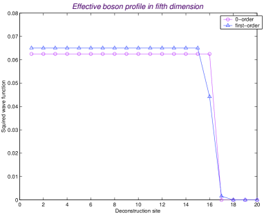
Figure 1: The wave-function profile of the effective gauge boson, up to zero and first order in perturbation theory in $\delta$. The numerical values are $N_{E}=15$ and $\delta=0.17$

The effective gauge boson penetrates deeper into the fifth dimension as the energy is lowered. At low energies, the scattering is mediated by the zero mode, which penetrates all the way down to the TeV brane, and contains gauge bosons from all sites with equal weights. At higher energies $E$, in the coarse lattice limit, the effective gauge boson is an equal-weight combination of $N_{E}$ gauge bosons corresponding to sites adjacent to the Planck brane. This picture justifies the energy-dependent cutoff brane of [2]. Working with a finer lattice, we see that this step-function profile is actually “smeared”, and to ${\cal O}(\delta)$, the effective gauge boson now receives a small contribution from one additional site, namely $A_{N_{E}+2}$. At higher orders in perturbation theory, we will see more sites giving such small contributions, so that the step function profile becomes smooth.

5 Conclusions and Outlook

In this paper, we studied a deconstructed AdS₅ gauge theory, focusing on fine latticization, with the inverse lattice spacing comparable to the curvature. The fact that we obtained a general result for the product of all non-zero KK-masses, allowed us to write down an expression for the coupling at low energies, which is valid for any curvature and lattice spacing. Thus, formally at least, this expression interpolates between the flat case and strongly warped case.

At one-loop, for finite warping, we find, apart from the well-known logarithmic piece, a contribution that scales linearly with the cutoff. This contribution is not universal—it involves the one-loop beta function coefficient of the theory.

We then discuss the gauge boson propagator at intermediate energies, using perturbation theory around the coarse lattice limit. However, we find that even using this perturbation theory, it is very hard to analytically calculate loop corrections to the propagator. Furthermore, in the regime in which we can trust the approximation, the number of KK modes in a given energy interval is not corrected. Therefore, we cannot see any qualitative modification of the gauge coupling scale dependence compared to the coarse lattice result. It will be interesting to study these issues numerically, and we leave this analysis for future work.

It will also be interesting to extend our results to theories containing bulk matter fields, and in particular, to consider the deconstruction of realistic GUT models, with GUT breaking by either boundary conditions or by a bulk Higgs field.

6 Acknowledgements

We thank A. Delgado, T. Gherghetta, and especially Y. Shirman for useful discussions. We also thank N. Arkani-Hamed, L. Randall and N. Weiner for discussions that inspired this work. This research was supported in part by the Israel Science Foundation (ISF) under grant 29/03, and by the United States-Israel Science Foundation (BSF) under grant 2002020.

Appendix A Mass eigenvalues and eigenstates

Here we diagonalize the gauge boson mass matrix (9). We consider a coarse lattice with $\kappa\mathrel{\hbox to0.0pt{\lower 4.0pt\hbox{\hskip 1.0pt$\sim$}\hss}\raise 1.0pt\hbox{$>$}}v$, and define the hierarchy parameter:

$$\delta\equiv\frac{v_{j}^{2}}{v_{j-1}^{2}}~{}.$$ (34)

In the limit $k\rightarrow\infty$, $\delta$ goes to zero as does the ratio of adjacent VEVS. In the following we will obtain the gauge boson masses and eigenstates as an expansion in $\delta$ around this limit.

We first write ${\cal M}^{2}$ as the sum of operators:

$${\cal M}^{2}=\sum_{j=1}^{N-1}{\cal M}_{j}^{2}~{}.$$ (35)

These operators act on the original (site) states as

$${\cal M}_{j}^{2}|A_{j}\rangle = v_{j}^{2}\left(|A_{j}\rangle-|A_{j+1}\rangle\right)~{};$$ (36)

$${\cal M}_{j}^{2}|A_{j+1}\rangle = v_{j}^{2}\left(-|A_{j}\rangle+|A_{j+1}\rangle\right)~{};$$

$${\cal M}_{j}^{2}|A_{l}\rangle = 0\quad\forall l\neq j,j+1~{}.$$

Since we assume a coarse lattice, the operator ${\cal M}_{1}^{2}$ can be treated as the leading operator and all other operators as perturbations.

The eigenstates of ${\cal M}_{1}^{2}$ are:

$$\left|B_{1}\right\rangle = \sqrt{\frac{1}{2}}\left(-\left|A_{1}\right\rangle+\left|A_{2}\right\rangle\right)~{};$$ (37)

$$\left|B_{{m=0}}^{1}\right\rangle = \sqrt{\frac{1}{2}}\left(\left|A_{1}\right\rangle+\left|A_{2}\right\rangle\right)~{},$$

of masses-squared $2v_{1}^{2}$ and zero respectively. So at this stage, we have $N-1$ degenerate massless states. This degeneracy is lifted by the operator ${\cal M}_{2}^{2}$.

Iterating this procedure, we find that the operator ${\cal M}_{j}^{2}$ , treated as a perturbation, removes the degeneracy between the states $\left|A_{j+1}\right\rangle$ and $\left|B_{m=0}^{j-1}\right\rangle=\frac{1}{\sqrt{j}}\sum_{k=1}^{j+1}\left|A_{k}\right\rangle$. The matrix elements of this operator ${\cal M}_{j}^{2}$ in the sub-space of degeneracy are:

$$\left\langle A_{j+1}\right|{\cal M}_{j}^{2}\left|A_{j+1}\right\rangle = v_{j}^{2}~{};$$ (38)

$$\left\langle B_{m=0}^{j-1}\right|{\cal M}_{j}^{2}\left|B_{m=0}^{j-1}\right\rangle = \frac{v_{j}^{2}}{j}~{};$$

$$\left\langle A_{j+1}\right|{\cal M}_{j}^{2}\left|B_{m=0}^{j-1}\right\rangle = -\frac{v_{j}^{2}}{\sqrt{j}}~{}.$$

To leading order, the masses are then,

$$m_{j}^{2}=v_{j}^{2}\frac{j+1}{j}~{},$$ (39)

and solving for the eigenstates we find,

$$\left|B_{j}\right\rangle = \sqrt{\frac{j}{j+1}}\left(\left|A_{j+1}\right\rangle-\frac{1}{j}\sum_{k=1}^{j}\left|A_{k}\right\rangle\right)\qquad j=1\ldots N-1~{};$$ (40)

$$\left|B_{m=0}^{final}\right\rangle = \sqrt{\frac{1}{N}}\sum_{k=1}^{N}\left|A_{k}\right\rangle~{}.$$

Equations (39) and (40) give the infinite-curvature result. We now want to calculate corrections to these result for finite curvature. That is, we will now derive the masses-squared and eigenstates to order ${\cal O}(\delta)$. The ${\cal O}(\delta)$ correction to each eigenmass can come either from including the second order in ${\cal M}_{j}^{2}$, or from first order in ${\cal M}_{j+1}^{2}$. Note that the last eigenstate, $\left|B_{m=0}^{final}\right\rangle$ is an exact eigenstate of the mass matrix with the zero mass for any curvature, and therefore should not get corrected.

The second order ${\cal M}_{j}^{2}$ correction is

$$\Delta m_{j}^{2}=\sum_{k<j}\frac{\left|\left\langle B_{j}\right|{\cal M}_{j}^{2}\left|B_{k}\right\rangle\right|^{2}}{m_{j}^{2}-m_{k}^{2}}~{}.$$ (41)

with

$$\left\langle B_{j}\right|{\cal M}_{j}^{2}\left|B_{j-1}\right\rangle = -v_{j}^{2}\frac{\sqrt{(j-1)(j+1)}}{j}~{};$$ (42)

$$\left\langle B_{j}\right|{\cal M}_{j}^{2}\left|B_{k}\right\rangle = 0\quad\forall k<j-1~{},$$

so there is only one non-zero matrix element the numerator of (41)numerator sum. The denominator contribution is:

$$\frac{1}{m_{j}^{2}-m_{j-1}^{2}}=\frac{-1}{\frac{j}{j-1}v_{j-1}^{2}}\left(1+\frac{(j+1)(j-1)}{j^{2}}\delta+\ldots\right)~{},$$ (43)

so that eqn. (41) becomes

$$\Delta m_{j}^{2}=\frac{(j-1)(j+1)}{j^{2}}v_{j}^{4}\left(\frac{-1}{\frac{j}{(j-1)}v_{j-1}^{2}}+{\cal O}(\delta)\right)=-\frac{(j-1)^{2}(j+1)}{j^{3}}v_{j}^{2}\delta+{\cal O}((\delta)^{2})~{}.$$ (44)

The contribution of the operator ${\cal M}^{2}_{j+1}$ is:

$$\Delta m_{j}^{2}=\langle B_{j}|{\cal M}^{2}_{j+1}|B_{j}\rangle=\frac{j}{j+1}v_{j}^{2}\delta~{}.$$ (45)

Together (44) and (45) give the total first-order correction to the mass-squared eigenvalue

$$\Delta m_{j}^{2}=v_{j}^{2}\left(\frac{j}{j+1}-\frac{(j-1)^{2}(j+1)}{j^{3}}\right)\delta~{}.$$ (46)

Adding this to the leading result we find

$$m_{j}^{2}=v_{j}^{2}\left[\frac{j+1}{j}+\delta\left(\frac{j}{j+1}-\frac{(j-1)^{2}(j+1)}{j^{3}}\right)\right]+{\cal O}(\delta^{2})~{},$$ (47)

or in more convenient form

$$m_{j}^{2}=v_{j}^{2}\left(\frac{j+1}{j}\right)\left[1+\delta\frac{2j^{2}-1}{j^{2}(j+1)^{2}}+{\cal O}(\delta^{2})\right]~{}.$$ (48)

The leading order correction to the eigenstates likewise comes from two powers of the operator ${\cal M}_{j}^{2}$ and one power of ${\cal M}_{j+1}^{2}$,

$$\left|B_{j}^{1}\right\rangle=\left|B_{j}^{0}\right\rangle+\sum_{k\neq j}\left|B_{k}^{0}\right\rangle\frac{\left\langle B_{k}^{0}\right|{\cal M}_{j}^{2}\left|B_{j}^{0}\right\rangle}{m_{j}^{2}-m_{k}^{2}}+\sum_{k\neq j}\left|B_{k}^{0}\right\rangle\frac{\left\langle B_{k}^{0}\right|{\cal M}_{j+1}^{2}\left|B_{j}^{0}\right\rangle}{m_{j}^{2}-m_{k}^{2}}~{},$$ (49)

where the masses are taken up to zero order in $\delta$.

Using the results of the previous calculation we obtain the following form of mass matrix eigenstates:

$$\left|B_{j}^{1}\right\rangle=\left|B_{j}^{0}\right\rangle+\delta\sqrt{\frac{(j-1)^{3}(j+1)}{j^{4}}}\left|B_{j-1}^{0}\right\rangle-\delta\sqrt{\frac{j^{3}(j+2)}{(j+1)^{4}}}\left|B_{j+1}^{0}\right\rangle+{\cal O}((\delta)^{2})~{}.$$ (50)

One can easily check that, to ${\cal O}(\delta)$, these eigenstates satisfy

$$\langle B_{j}|B_{k}\rangle=\delta_{jk}~{}.$$ (51)

Appendix B Calculating the product of nonzero masses

We now want to calculate the product of all non-zero masses. To do so, we will use the basis $|B_{j}^{0}\rangle$ of eqn (40). While this basis does not diagonalize the mass matrix for finite curvature, it is nonetheless useful for our purposes, since it decouples the massless mode while leaving a remaining block which is a regular matrix with all the required information about the massive KK modes.

To calculate the matrix elements in this remaining block we use the division introduced in (35). In general the action of the operator ${\cal M}_{j}^{2}$ on the basis $|B_{j}\rangle$ has the following form:

$${\cal M}^{2}_{j}|B_{l}\rangle=\sqrt{\frac{l}{l+1}}\left({\cal M}^{2}_{j}|A_{l+1}\rangle-\frac{1}{l}\sum_{k=1}^{l}{\cal M}_{j}^{2}|A_{k}\rangle\right)~{}.$$ (52)

One can easily see that the second part of this expression is non-zero only if $j=l$:

$$\sum_{k=1}^{l}{\cal M}_{j}^{2}|A_{k}\rangle=v_{j}^{2}\delta_{jl}\left(|A_{j}\rangle-|A_{j+1}\rangle\right)~{}.$$ (53)

Using (36) and (53) one obtains

$${\cal M}_{j}^{2}|B_{j}\rangle = v_{j}^{2}\sqrt{\frac{j+1}{j}}\left(-|A_{j}\rangle+|A_{j+1}\rangle\right)~{};$$ (54)

$${\cal M}_{j}^{2}|B_{j-1}\rangle = v_{j}^{2}\sqrt{\frac{j-1}{j}}\left(|A_{j}\rangle-|A_{j+1}\rangle\right)~{};$$ (55)

$${\cal M}_{j}^{2}|B_{l}\rangle = 0\quad\quad\forall l\neq j,j-1~{}.$$ (56)

Since the operator ${\cal M}_{j}^{2}$ is Hermitian, we conclude that it has only three different non-zero matrix elements in the $|B_{j}\rangle$ basis, which are (for $j\neq 1)$,

$$\langle B_{j}|{\cal M}_{j}^{2}|B_{j}\rangle = \frac{j+1}{j}v_{j}^{2}~{};$$ (57)

$$\langle B_{j-1}|{\cal M}_{j}^{2}|B_{j-1}\rangle = \frac{j-1}{j}v_{j}^{2}~{};$$ (58)

$$\langle B_{j}|{\cal M}_{j}^{2}|B_{j-1}\rangle=\langle B_{j-1}|{\cal M}_{j}^{2}|B_{j}\rangle = -\frac{\sqrt{(j-1)(j+1)}}{j}v_{j}^{2}~{}.$$ (59)

For $j=1$ we have only one non-zero element,

$$\langle B_{1}|{\cal M}_{1}^{2}|B_{1}\rangle=2v_{1}^{2}~{}.$$ (60)

Thus, in this basis, the zero mode is explicitly decoupled, and the product of KK-masses is just a determinant of the upper left $(N-1)\times(N-1)$ block. We can call this $(N-1)\times(N-1)$ matrix the “reduced matrix”, or ${\cal M}^{2}_{red}$, its explicit matrix form is:

$${\cal M}^{2}_{red}=\left(\begin{array}[]{cccccc}2v_{1}^{2}+\frac{1}{2}v_{2}^{2}&-\frac{\sqrt{3}}{2}v_{2}^{2}&&&&\\ -\frac{\sqrt{3}}{2}v_{2}^{2}&\frac{3}{2}v_{2}^{2}+\frac{2}{3}v_{3}^{2}&\ddots&&&\\ &\ddots&\ddots&\ddots&&\\ &&\ddots&\frac{j}{j-1}v_{j-1}^{2}+\frac{j-1}{j}v_{j}^{2}&-\frac{\sqrt{(j-1)(j+1)}}{j}v_{j}^{2}&\\ &&&-\frac{\sqrt{(j-1)(j+1)}}{j}v_{j}^{2}&\frac{j+1}{j}v_{j}^{2}+\frac{j}{j+1}v_{j+1}^{2}&\ddots\\ &&&&\ddots&\ddots\end{array}\right)$$ (61)

We then have

$$\det{\cal M}^{2}_{red}=\det{\cal M}_{N-1}^{2}\det\sum_{j=1}^{N-3}{\cal M}_{j}^{2}+{\cal M}^{2}_{(N-1)(N-1)}\det\sum_{j=1}^{N-2}{\cal M}_{j}^{2}~{}.$$ (62)

Using the fact that

$$\det{\cal M}_{j}^{2}=0\qquad\forall j~{},$$ (63)

we are left with only one non-zero term on the LHS of (62). Iterating this procedure for the other rows of this matrix we finally obtain the desired determinant

$$\det{{\cal M}}_{red}^{2}=\prod_{j=1}^{N-1}\frac{j+1}{j}v_{j}^{2}=N\prod_{j=1}^{N-1}v_{j}^{2}~{}.$$ (64)

References

- [1] A. Pomarol, Phys. Rev. Lett. 85, 4004 (2000) [arXiv:hep-ph/0005293];
- [2] L. Randall and M. D. Schwartz, JHEP 0111, 003 (2001) [arXiv:hep-th/0108114].
- [3] L. Randall and M. D. Schwartz, Phys. Rev. Lett. 88, 081801 (2002) [arXiv:hep-th/0108115].
- [4] K. Agashe, A. Delgado and R. Sundrum, Nucl. Phys. B 643, 172 (2002) [arXiv:hep-ph/0206099];
- [5] K. w. Choi and I. W. Kim, Phys. Rev. D 67, 045005 (2003) [arXiv:hep-th/0208071]; K. w. Choi, H. D. Kim and I. W. Kim, JHEP 0303, 034 (2003) [arXiv:hep-ph/0207013].
- [6] W. D. Goldberger and I. Z. Rothstein, Phys. Rev. Lett. 89, 131601 (2002) [arXiv:hep-th/0204160]; W. D. Goldberger and I. Z. Rothstein, Phys. Rev. D 68, 125011 (2003) [arXiv:hep-th/0208060]; R. Contino, P. Creminelli and E. Trincherini, JHEP 0210, 029 (2002) [arXiv:hep-th/0208002].
- [7] W. D. Goldberger and I. Z. Rothstein, Phys. Rev. D 68, 125012 (2003) [arXiv:hep-ph/0303158].
- [8] L. Randall and R. Sundrum, Phys. Rev. Lett. 83, 3370 (1999) [arXiv:hep-ph/9905221].
- [9] N. Arkani-Hamed, A. G. Cohen and H. Georgi, Phys. Rev. Lett. 86, 4757 (2001) [arXiv:hep-th/0104005]; C. T. Hill, S. Pokorski and J. Wang, Phys. Rev. D 64, 105005 (2001) [arXiv:hep-th/0104035].
- [10] H. Abe, T. Kobayashi, N. Maru and K. Yoshioka, Phys. Rev. D 67, 045019 (2003) [arXiv:hep-ph/0205344]; H. C. Cheng, C. T. Hill and J. Wang, Phys. Rev. D 64, 095003 (2001) [arXiv:hep-ph/0105323].
- [11] L. Randall, Y. Shadmi and N. Weiner, JHEP 0301, 055 (2003) [arXiv:hep-th/0208120].
- [12] A. Falkowski and H. D. Kim, JHEP 0208, 052 (2002) [arXiv:hep-ph/0208058].