Basic results in Vacuum Statistics

Abstract

A review of recent work on constructing and finding statistics of string theory vacua, done in collaboration with Frederik Denef, Bogdan Florea, Bernard Shiffman and Steve Zelditch.

To appear in the proceedings of Strings 2004, June 28-July 2, Paris, France.

Tout ce qui est simple est faux, mais tout ce qui ne l’est pas est inutilisable.

– Paul Valéry

1 Predictions from string theory

For almost 20 years we have had good qualitative arguments that compactification of string theory can reproduce the Standard Model and solve its problems, such as the hierarchy problem. But we still seek distinctive predictions which we could regard as evidence for or against the theory.

One early spin-off of string theory, four dimensional supersymmetry, is the foundation of most current thinking in “beyond the Standard Model” physics. Low energy supersymmetry appears to fit well with string compactification. But would not discovering supersymmetry be evidence against string/M theory?

In recent years, even more dramatic possibilities have been suggested, which would lead to new, distinctive particles or phenomena: large extra dimensions (KK modes); a low fundamental string scale (massive string modes); rapidly varying warp factors (modes bound to branes; conformal subsectors), and so on. Any of these could lead to dramatic discoveries. But should we expect string/M theory to lead to any of these possibilities? Would not discovering them be evidence against string theory?

At Strings 2003, I discussed a statistical approach to these and other questions of string phenomenology. Over the last year, our group at Rutgers, and the Stanford group, have made major progress in developing this approach, with

• Explicit proposals for vacua with all moduli stabilized along the lines of KKLT [27] (work with Denef and Florea [12]).

• Detailed results for distributions of these vacua (with Shiffman, Zelditch and Denef [17, 11])

• Preliminary results on the statistics of the volume of the extra dimensions (in progress with Denef), and on supersymmetry breaking scales [18, 13, 35].

These ideas have already begun to inspire new phenomenological models (for example [3, 22]). Even better, if we are lucky and the number of vacua is not too large (as we explain below), fairly convincing predictions might come out of this approach over the next few years. While much work would be needed to bring this about, we may be close to making some predictions: those which use just the most generic features of string/M theory compactification, namely the existence of many hidden sectors.

2 Hidden sectors

Before string theory, and during the “first superstring revolution,” most thinking on unified theories assumed that internal consistency of the theory would single out the matter content we see in the real world. In the early 1980’s it was thought that $d=11$ supergravity might do this. Much of the early excitement about the heterotic string came from the fact that it could easily produce the matter content of $E_{6}$, $SO(10)$ or $SU(5)$ grand unified theory.

But this was not looking at the whole theory. The typical compactification of heterotic or type II strings on a Calabi-Yau manifold has hundreds of scalar fields, larger gauge groups and more charged matter. Already in the perturbative heterotic string an extra $E_{8}$ appeared. With branes and non-perturbative gauge symmetry, far larger groups are possible, with many simple factors. If we live in a “typical” string compactification, it seems that there are many hidden sectors, not directly visible to observation or experiment.

Should we care? Does this lead to any general predictions? Hidden sectors may or may not lead to new particles or forces. But what they do generically lead to is a multiplicity of vacua, because of symmetry breaking, choice of vev of additional scalar fields, or other discrete choices.

Let us say a hidden sector allows $c$ distinct vacua or “phases.” If there are $N$ hidden sectors, the multiplicity of vacua will go as

$${\cal N}_{vac}\sim c^{N}.$$

While the many hidden sectors certainly make the detailed study of string compactification more complicated, we should consider the idea that they lead to simplifications as well. Thus we might ask, what can we say about the case of a large number $N$ of hidden sectors ? Clearly there will be a large multiplicity of vacua.

We only live in one vacuum. However, as pointed out by Brown and Teitelboim [9], Banks, Dine and Seiberg [5], and no doubt many others, vacuum multiplicity can help in solving the cosmological constant (c.c.) problem. In an ensemble of ${\cal N}_{vac}$ vacua with roughly uniformly distributed c.c. $\Lambda$, one expects that vacua will exist with $\Lambda$ as small as $M_{pl}^{4}/{\cal N}_{vac}$. To obtain the observed small nonzero c.c. $\Lambda\sim 10^{-122}M_{pl}^{4}$, one requires ${\cal N}_{vac}>10^{120}$ or so.

Now, assuming different phases have different vacuum energies, adding the energies from different hidden sectors can produce roughly uniform distributions. In fact, the necessary ${\cal N}_{vac}$ can easily be fit with ${\cal N}_{vac}\sim c^{N}$ and the parameters $c\sim 10$, $N\sim 100-500$ one expects from flux compactification of string theory, as first argued by Bousso and Polchinski [8].

One might regard fitting the observed small nonzero c.c. in any otherwise acceptable vacuum as solving the problem, or one might appeal to an anthropic argument such as that of Weinberg [36] to select this vacuum. In the absence of other candidate solutions to the problem, we might even turn this around and call these ideas evidence for the hypothesis that we are in a compactification with many hidden sectors.

3 Supersymmetry breaking

So can we go further with these ideas? Another quantity which can get additive contributions from different sectors is the scale of supersymmetry breaking. Let us call this $M_{susy}^{2}$ (we will define it more carefully below).

We recall the classic arguments for low energy supersymmetry from naturalness. The electroweak scale $m_{EW}$ is far below the other scales in nature $M_{pl}$ and $M_{GUT}$. According to one definition of naturalness, this is only to be expected if a symmetry is restored in the limit $m_{EW}\rightarrow 0$. This is not true if $m_{EW}$ is controlled by a scalar (Higgs) mass $m_{H}$, but can be true if the Higgs has a supersymmetric partner (we then restore a chiral symmetry).

A more general definition of naturalness requires the theory to be stable under radiative corrections, so that the small quantity does not require fine tuning. Again, low energy supersymmetry can accomplish this. Many theories have been constructed in which

$$M_{H}^{2}\sim cM_{susy}^{2},$$

with $c\sim 1/10$ without fine tuning. Present data typically requires $c<1/100$, which requires a small fine tuning (the “little hierarchy problem.”)

On the other hand, the solution to the cosmological constant problem we accepted above, in terms of a discretuum of vacua, is suspiciously similar to fine tuning the c.c., putting the role of naturalness in doubt. What should replace it?

The original intuition of string theorists was that string theory would lead to a unique four dimensional vacuum state, or at most very few, such that only one would be a candidate to describe real world physics. In this situation, there is no clear reason the unique theory should be “natural” in the previously understood sense.

With the development of string compactification, it has become increasingly clear that there is a large multiplicity of vacua. The vacua differ not only in the cosmological constant, but in every possible way: gauge group, matter content, couplings, etc. What should we do in this situation?

The “obvious” thing to do at present is to make the following definition [15]:

An effective field theory (or specific coupling, or observable) $T_{1}$ is more natural in string theory than $T_{2}$, if the number of phenomenologically acceptable vacua leading to $T_{1}$ is larger than the number leading to $T_{2}$.

Now there is some ambiguity in defining “phenomenologically acceptable” (or even “anthropically acceptable,” as some would have it [34]). One clearly wants $d=4$, supersymmetry breaking, etc. One may or may not want to put in more detailed information from the start.

In any case, the unambiguously defined information provided by string/M theory is the number of vacua and the distribution of resulting EFT’s. For example, we could define

$$d\mu[M_{H}^{2},M_{susy}^{2},\Lambda]=\rho(M_{H}^{2},M_{susy}^{2},\Lambda)dM_{H}^{2}\ dM_{susy}^{2}\ d\Lambda\hfill$$

$$=\sum_{T_{i}}\delta(M_{susy}^{2}-M_{susy}^{2}|_{T_{i}})\delta(M_{H}^{2}-M_{H}^{2}|_{T_{i}})\delta(\Lambda-\Lambda|_{T_{i}})$$

a distribution which counts vacua with given c.c., susy breaking scale and Higgs mass, and study the function

$$\rho(10^{4}\leavevmode\nobreak\ {\rm GeV}^{2},M_{susy}^{2},\Lambda\sim 0).$$

4 Statistical selection

Is this definition of “stringy naturalness” good for anything? Suppose property $X$ (say low scale susy) were realized by $10^{40}$ phenomenologically acceptable vacua, while $\bar{X}$ (say high scale susy) were realized by $10^{20}$ such vacua. If by prediction we mean not just a hunch or a reason to bet on a particular property, but a property whose observation would actually falsify string theory (and this is what we really need in the end), we should not conclude that string theory predicts low scale susy.

On the other hand, if the distribution is sharply enough peaked, and there are not too many vacua, it could well turn out that some regions of theory space would have no vacua, and we would get a prediction.

For example, suppose there were $10^{160}$ vacua with the property $X$ (say low scale susy), and which realize all known physics, except for the observed c.c.. Suppose further that they realize a uniform distribution of cosmological constants; then out of this set we would expect about $10^{40}$ to also reproduce the observed cosmological constant. Suppose furthermore that $10^{100}$ vacua with property $\bar{X}$ work except for possibly the c.c.; out of this set we only expect the correct c.c. to come out if an additional $10^{-20}$ fine tuning is present in one of the vacua which comes close. Not having any reason to expect this, and having other vacua which work, we have reasonable grounds for predicting $X$, in the strong sense that observing $\bar{X}$ would be evidence against string theory.

In a systematic approach, one would take all aspects of the physics resulting from each choice of vacuum, not just the c.c. but couplings and matter content as well, and make the analogous argument. As discussed in [15], the rest of the information at hand is comparable in selectivity to the c.c.; say a rough fraction $10^{-240}$ of vacua out of a fairly uniform ensemble might reproduce the Standard Model, and thus this is an important improvement. However the basic idea leading to predictions is more or less the same.

Upon considering the entire problem in this way, the most crucial advantage of the statistical approach becomes apparent. It is that we can benefit by the hypothesis that some properties of the distribution of vacua are (to a good approximation) statistically independent, in which case we can argue that vacua exist which realize a group of properties simultaneously, even without finding explicit examples.

For example, it seems very likely that the value of the c.c. is independent of the number of Standard Model generations, in the sense that even if we restrict attention to vacua with a given number $N_{gen}$ of generations we will still find a uniform distribution of c.c.’s with cutoff independent of $N_{gen}$. Then, suppose for sake of argument that a fraction $10^{-4}$ of the vacua have $N_{gen}=3$. While not rare compared to other properties, this is sufficiently rare to make it significantly more difficult to find models with both $N_{gen}=3$ and the small c.c.. Rather than do this, we should study the larger population of models with arbitrary $N_{gen}$ and check the hypothesis that these properties are independent. Having done this, we can argue that the fraction of vacua which realize both properties is the product of the fractions which realize each, without explicitly finding the vacua which realize both. Of course, the independence hypothesis might turn out to be false; if we found evidence of a correlation between $N_{gen}$ and the c.c., that would be even more interesting (and surprising).

We can go on to make the same type of analysis for each of the characteristic properties of the Standard Model (the gauge group, the hierarchy, the details of the couplings and so on). While any one of its specific properties is “rare” in the sense that the great majority of vacua do not realize it (most vacua will not have unbroken gauge symmetry at low energy, etc.), it seems unlikely that any one of them (even the c.c.) is so rare as to allow only a few candidate vacua. Multiplying the fractions of vacua which realize the various properties leads to an estimated fraction of vacua which agree with the Standard Model, finite but so small that the task of finding the vacuum which actually realizes all of its properties simultaneously is almost impossible. On the other hand, by separating the various properties of interest into subsets, such that correlations are possible only within each subset, we can hope to divide up the problem into manageable pieces.

These arguments and examples illustrate how, under certain possible outcomes for the actual number and distribution of vacua, we could make well motivated predictions. Of course the actual numbers and distribution are not up to us to chose, and one can equally well imagine scenarios in which this type of predictivity is not possible. For example, ${\cal N}_{vac}\sim 10^{1000}$ would probably not lead to predictions, unless the distribution were very sharply peaked, or unless we make further assumptions which drastically cut down the number of vacua.

5 Absolute numbers

The basic estimate for numbers of flux vacua [4] is

$${\cal N}_{vac}\sim\frac{(2\pi L)^{K/2}}{(K/2)!}[c_{n}]$$

where $K$ is the number of distinct fluxes ($K=2b_{3}$ for IIb on CY₃) and $L$ is a “tadpole charge” ($L=\chi/24$ in terms of the related CY₄). The “geometric factor” $[c_{n}]$ does not change this much, while other multiplicities are probably subdominant to this one.

Typical $K\sim 100-400$ and $L\sim 500-5000$, leading to ${\cal N}_{vac}\sim 10^{500}$. This is probably too large for statistical selection to work.

On the other hand, this estimate did not put in all the consistency conditions. Here are two ideas, still rather speculative.

• Perhaps stabilizing the moduli not yet considered in detail (e.g. brane moduli) is highly non-generic, or perhaps most of the flux vacua become unstable after supersymmetry breaking due to KK or stringy modes becoming tachyonic. At present there is no evidence for these ideas, but neither have they been ruled out.

• Perhaps cosmological selection is important: almost all vacua have negligible probability to come from the “preferred initial conditions.” Negligible means $P<<<1/{\cal N}_{vac}$, and almost all existing proposals for wave functions or probabilty factors are not so highly peaked, but eternal inflation has been claimed to be (as reviewed in [26]), and it is important to know if this is relevant for string theory (see for example [20]).

Such considerations might drastically cut the number of vacua. While we would then need to incorporate these effects in the distribution, it is conceivable that to a good approximation these effects are statistically independent of the properties of the distribution which concern us, so that the statistics we are computing now are the relevant ones. Even if not, it seems very unlikely to us that cosmology will select a unique vacuum a priori; rather we believe the problem with these considerations taken into account will not look so different formally (and perhaps even physically) from the problem without them, and thus we proceed.

6 Stringy naturalness

The upshot of the previous discussion is that in this picture, either string theory is not predictive because there are too many vacua, or else the key to making predictions is to count vacua, find their distributions, and apply the principles of statistical selection.

To summarize this, we again oversimplify and describe statistical selection as follows: we propose to show that a property $\bar{X}$ cannot come out of string theory by arguing that no vacuum realizing $\bar{X}$ reproduces the observed small c.c. (actually, we are considering all properties along with the c.c.). One might ask how we can hope to do this, given that computing the c.c. in a specific vacuum to the required accuracy is far beyond our abilities. The point is that it should be far easier to characterize the distribution of c.c.’s than to compute the c.c. in any specific vacuum. To illustrate, suppose we can compute it at tree level, but that these results receive complicated perturbative and non-perturbative corrections. Rather than compute these exactly in each vacuum, we could try to show that they are uncorrelated with the tree level c.c.; if true and if the tree level distribution is simple (say uniform), the final distribution will also be simple.

If so, tractable approximations to the true distribution of vacua can estimate how much unexplained fine tuning is required to achieve the desired EFT, and this is the underlying significance of the definition of “stringy naturalness” we gave above.

Thus, we need to establish that vacua satisfying the various requirements exist, and estimate their distribution. We now discuss results on these two problems, and finally return to the question of the distribution of supersymmetry breaking scales.

7 Constructing KKLT vacua

The problem of stabilizing all moduli in a concrete way in string compactification has been studied for almost 20 years. One of the early approaches was to derive an effective Lagrangian by KK reduction, find a limit in which nonperturbative effects are small, and add sufficiently many nonperturbative corrections to produce a generic effective potential. Such a generic potential, depending on all moduli, will have isolated minima. While the idea is simple, the complexities of string compactification and the presence of hundreds of moduli have made it hard to carry out.

A big step forward was the development of flux compactification by Polchinski and Strominger [30]; Becker and Becker [7]; Dasgupta, Rajesh and Sethi [10], and many others. Since the energy of fluxes in the compactification manifold depends on moduli, turning on flux allows stabilizing a large subset of moduli at the classical level. Acharya [1] has proposed that in $G_{2}$ compactification, all metric moduli could be stabilized by fluxes. However it is not yet known how to make explicit computations in this framework.

The most computable class of flux compactifications at present is that of Giddings, Kachru and Polchinski [21], in IIb orientifold compactification, because one can appeal to the highly developed theory of Calabi-Yau moduli spaces and periods. However the IIb flux superpotential does not depend on Kähler moduli, nor does it depend on brane or bundle moduli. Now one can argue that the brane/bundle moduli parameterize compact moduli spaces (e.g. consider the D3 brane), and thus they will be stabilized by a generic effective potential. However, for the Kähler moduli, we need to show that the minimum is not at infinite volume, or deep in the stringy regime (in which case we lose control). Thus we need a fairly explicit expression for their effective potential.

Kachru, Kallosh, Linde and Trivedi (KKLT) [27] proposed to combine the flux superpotential with

• a nonperturbative superpotential produced by D3 instantons and/or D7 world-volume gauge theory effects. These depend on Kähler moduli and can in principle fix them.

• energy from an anti-D3 brane, which would break supersymmetry and lift the c.c. to a small positive value.

However they did not propose a concrete model which contained these effects, and in fact such models are not so simple to find. The main problem is that most brane gauge theories in compactifications which cancel tadpoles, have too much matter to generate superpotentials. One needs systematic techniques to determine this matter content, or compute instanton corrections, and find the examples which work.

In [12], Denef, Florea and I found the first examples which work. Our construction relies heavily on the analysis of instanton corrections in F theory due to Witten [37], Donagi and especially A. Grassi [24]. Their starting point was to compactify M theory on a Calabi-Yau fourfold $X$. This leads to a 3D theory with four supercharges, related to F theory and IIb if $X$ is $T^{2}$-fibered, by taking the limit ${\rm vol}(T^{2})\rightarrow 0$. The complex modulus of the $T^{2}$ becomes the dilaton-axion varying on the base $B$.

In M theory, an M5 brane wrapped on a divisor $D$ (essentially, a hypersurface), will produce a nonperturbative superpotential, if $D$ has arithmetic genus one:

$$1=\chi({\cal O}_{D})=h^{0,0}-h^{0,1}+h^{0,2}-h^{0,3}.$$

Each of these complex cohomology groups leads to two fermion zero modes; an instanton contributes to $W$ if there are exactly two. A known subset of these (vertical divisors) survive in F theory.

In the F theory limit, only divisors which wrap the $T^{2}$ contribute, and these correspond to D3-instantons wrapping surfaces in $B$. Thus, we looked for F theory compactifications on an elliptically fibered fourfold $X$ with enough divisors of arithmetic genus one, so that a superpotential

$$W=W_{flux}+\sum_{i}b_{i}e^{-\vec{t}\cdot D_{i}}$$

will lead to non-trivial solutions to $DW=0$ by balancing the exponentials against the dependence coming from the Kähler potential.

In the math literature, there is a very general relation between divisors of a.g. one, and contractions of manifolds. It implies that no model with one Kähler modulus can stabilize Kähler moduli (see also [32]), at least by using a.g. one divisors. Now there may be ways beyond the a.g. one condition: Witten [37] suggested that $\chi(D)>1$ might work as well (without providing examples); furthermore Gorlich et al [23] have argued that flux lifts additional matter and relaxes some of these constraints.

In any case, there is no problem if the CY threefold has more than one Kähler modulus, as in the vast majority of cases. Using the very complete study of divisors of a. g. one of A. Grassi [24], we have found $6$ models with toric Fano threefold base which can stabilize all Kähler moduli, and could be analyzed in detail using existing techniques.

The simplest, ${\cal F}_{18}$, has $89$ complex structure moduli. According to the AD counting formula, it should have roughly $\epsilon\times 10^{307}$ flux vacua with all moduli stabilized, where

$$\epsilon=g_{s}\times\frac{|W|^{2}}{m_{s}^{6}}\bigg{|}_{max}.$$

Models which stabilize all Kähler moduli using a.g. one divisors are not generic, but they are not uncommon either; there are 29 out of 92 with Fano base, and probably many more with ${\mathbb{P}}^{1}$ fibered base. This last class of model should be simpler, in part because they have heterotic duals, but analyzing them requires better working out the D7 world-volume theories. We also expect one can add antibranes or D breaking as in the KKLT discussion to get de Sitter vacua, but have not yet analyzed this.

8 Flux vacua

Figure 1: Values of $\tau$ for rigid CY flux vacua with $L_{max}=150$,from [11].

We recall the “flux superpotential” of Gukov, Taylor, Vafa and Witten in IIb string on CY,

$$W=\int\Omega(z)\wedge\left(F^{(3)}+\tau H^{(3)}\right).$$

The simplest example is to consider a rigid CY, i.e. with $b^{2,1}=0$ (for example, the orbifold $T^{6}/{Z}_{3}$). Then the only modulus is the dilaton $\tau$, with Kähler potential $K=-\log{\rm Im}\leavevmode\nobreak\ \tau$, and the flux superpotential reduces to

$$W=A\tau+B;\qquad A=a_{1}+\Pi a_{2};B=b_{1}+\Pi b_{2}$$

with $\Pi=\int_{\Sigma_{2}}\Omega^{(3)}/\int_{\Sigma_{1}}\Omega^{(3)}$, a constant determined by CY geometry.

Now it is easy to solve the equation $DW=0$:

$$DW =\frac{\partial W}{\partial\tau}-\frac{1}{\tau-\bar{\tau}}W =\frac{-A\bar{\tau}-B}{\tau-\bar{\tau}}$$

so $DW=0$ at $\bar{\tau}=-\frac{B}{A}$ where $\bar{\tau}$ is the complex conjugate.

The resulting set of flux vacua for $L=150$ and $\Pi=i$ is shown in Fig. 1. A similar enumeration for a Calabi-Yau with $n$ complex structure moduli, would produce a similar plot in $n+1$ complex dimensions, the distribution of flux vacua. It could (in principle) be mapped into the distribution of possible values of coupling constants in a physical theory.

This intricate distribution has some simple properties. For example, one can get exact results for the large $L$ asymptotics, by computing a continuous distribution $\rho(z,\tau;L)$, whose integral over a region $R$ in moduli space reproduces the asymptotic number of vacua which stabilize moduli in the region $R$, for large $L$,

$$\int_{R}dzd\tau\ \rho(z,\tau;\;L)\sim_{L\rightarrow\infty}N(R).$$

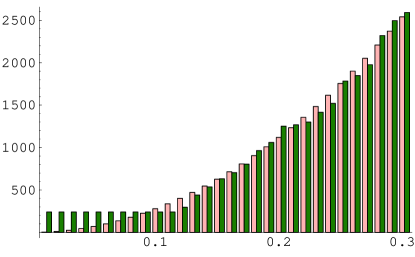
Figure 2: Number of vacua in a circle of coordinate radius $R$ around $\tau=2i$, with $R$ increasing in steps $dR=0.01$. Pink bars give the estimated value, green bars the actual value.

For a region of radius $r$, the continuous approximation should become good for $L>>K/r^{2}$. For example, if we consider a circle of radius $r$ around $\tau=2i$, we match on to the constant density distribution for $r>\sqrt{K/L}$, as we see in Fig. 2.

Explicit formulae for the continuous densities can be found, in terms of the geometry of the moduli space ${\cal C}$. The simplest such result [4] computes the index density of vacua:

$$\rho_{I}(z,\tau)=\frac{(2\pi L)^{b_{3}}}{b_{3}!\pi^{n+1}}\det(-R-\omega\cdot 1)$$

where $\omega$ is the Kähler form and $R$ is the matrix of curvature two-forms. Integrating this over a fundamental region of the moduli space produces an estimate for the total number of flux vacua. For example, for $T^{6}$ we found $I\sim 4\cdot 10^{21}$ for $L=32$. Since $r\sim 1$ in the bulk of moduli space, the condition $L>K/r^{2}$ for the validity of this estimate should be satisfied.

Another example is the “mirror quintic,” with a one parameter moduli space ${\cal M}_{c}(\tilde{Q})$ [11]. The integral is

$$\frac{1}{\pi^{2}}\int_{\cal C}\det(-R-\omega)=\frac{1}{12}\chi({\cal M}_{c}(\tilde{Q}))=\frac{1}{60}.$$

This density is “topological” and there are mathematical techniques for integrating it over general CY moduli spaces [29]. Good estimates for the index should become available for a large class of CY’s over the coming years.

9 Distributions of flux vacua

Figure 3: The susy vacuum number density per unit $\psi$ coordinate volume, $\pi\rho g_{\psi\bar{\psi}}/12$, on the real $\psi$-axis, for the mirror quintic.

In Fig. 3, we see the detailed distribution of flux vacua on the mirror quintic ($K=4$ and $n=1$), on a real slice through the complex structure moduli space [11]. Note the divergence at $\psi=1$. This is the conifold point, with a dual gauge theory interpretation. It arises because the curvature $R\sim\partial{\bar{\partial}}\log\log|\psi-1|^{2}$ diverges there. The divergence is integrable, but a finite fraction of all the flux vacua sit near it.

Quantitatively, for the mirror quintic,

• About $3\%$ of vacua sit near the conifold point, with an induced scale $|\psi-1|<10^{-3}$.

• About $1\%$ of vacua have $|\psi-1|<10^{-10}$. More generally, the density and number of vacua with $S\equiv\psi-1$ goes as

  $$\rho_{vac}\sim\frac{d^{2}S}{|S\log S|^{2}};\qquad{\cal N}_{vac}|_{S<S_{*}}\sim\frac{1}{|\log S_{*}|}.$$

  Writing $S=e^{-1/g^{2}}$, this is $\rho\sim d^{2}g/|g|^{2}$.

• About $36\%$ of vacua are in the “large complex structure limit,” defined as ${\rm Im}\leavevmode\nobreak\ t>2$ with $5\psi=e^{2\pi it/5}$. Here $\rho\sim d^{2}t/({\rm Im}\leavevmode\nobreak\ t)^{2}$.

Vacua close to conifold degenerations are interesting for model building, as they provide a natural mechanism for generating large hierarchies. We have found that such vacua are common, but are by no means the majority of vacua.

Note that some of these vacua have a dual gauge theory interpretation, while in other cases they should be thought of as supergravity backgrounds, possibly leading to Randall-Sundrum phenomenology [31]. The question of which interpretation is appropriate depends on the local parameter $g_{s}N$ where $N$ is the specific flux dual to the number of branes, and on the embedding of the Standard Model. It would be very interesting of course if one or the other alternative were strongly favored in the vacuum counting. Assuming the uniform distributions $dg_{s}$ and $dN$, one might expect a preference for $g_{s}N>1$ and Randall-Sundrum, but the ratio would seem to be at most of order $10^{2}-10^{3}$ which could easily be outweighed by other considerations. To do this right, one should also factor in the (model-dependent) relation between $g_{s}$ and the known (string scale) Standard Model couplings $g\sim 1/25$, which should lower the expected $g_{s}N$ and further weaken this preference.

Figure 4: The number density of susy vacua with positive mass matrix, per unit coordinate volume, on the real $\psi$-axis, for the mirror quintic. Compare to fig. 3.

Suppose we go on to break supersymmetry by adding an anti D3-brane, or by other D term effects. The previous analysis applies (since we have not changed the F terms), but now it is necessary that the mass matrix at the critical point is positive. The resulting distribution of tachyon-free D breaking vacua is given in Fig. 4. In fact, most D breaking vacua near the conifold point have tachyons (for one modulus CY’s), so we get suppression, not enhancement. This is not hard to understand in detail; the mechanism is a sort of “seesaw” mixing between modulus and dilaton, which seems special to one parameter models.

Figure 5: Left: Vacuum number densities (true and absolute value of index) in the large complex structure limit (${\cal F}=2/\sqrt{3}$), as a function of cosmological constant value, from [11]. Right: Same near the conifold limit (${\cal F}=100$ for this example).

In Fig. 5 one sees the distribution of (negative) AdS cosmological constants $\hat{\Lambda}=3e^{K}|W|^{2}$, both at generic points (left) and near the conifold point (right). Note that at generic points it is fairly uniform, all the way to the string scale. On the other hand, imposing small c.c. competes with the enhancement of vacua near the conifold point. The left hand graph compares the total number of vacua (green) with the index (red). The difference measures the number of Kähler stabilized vacua, vacua which exist because of the structure of the Kähler potential, not the superpotential.

10 Large complex structure/volume

Another simple universal property: given $n>>1$ moduli, the number of vacua falls off rapidly at large complex structure, or in a IIa mirror picture at large volume $V$, as

$$\int_{V>V_{0}}\rho\sim V_{0}^{-n/3}.$$

To see this, first note that $R\sim\omega$ in this regime, so the distribution of vacua is determined by the volume form derived from the metric on the space of metrics,

$$\left<\delta g_{ij},\delta g_{kl}\right>={1\over V}\int_{CY}\sqrt{g}g^{ik}g^{jl}\delta g_{ij}\delta g_{kl}$$

The $1/V$ factor (which compensates the $\sqrt{g}$) comes from the standard derivation of the kinetic term in KK reduction on CY. Because of the inverse factors of the metric, this falls off with volume as $V^{-1/3}$. Since the volume form is $\sqrt{G}$, this factor appears for each modulus. For large $n$, ${\cal N}\sim V^{-n/3}$ is a drastic falloff, and (as we saw explicitly in an example in [12]) typically there are no vacua in this regime.

A possible physical application of this: we know how to stabilize complex structure moduli using fluxes in IIb. Suppose we can use T-duality to get a corresponding class of models in IIa with stabilized Kähler moduli. Then, the mirror interpretation of this result is the number of vacua which stabilize the volume of the compact dimensions at a given value. Clearly large volume is highly unnatural in this construction, but do any vacua reach the $V\sim 10^{30}$ of the “large extra dimensions” scenario [2] ?

Writing $V\sim R^{6}$, we find a number of vacua

$$N\sim{(2\pi L)^{K}R^{-K}\over K!}$$

so large $K$ disfavors large volume in this case, and the maximum volume one expects is of order

$$V\sim\left({2\pi L\over K}\right)^{6}.$$

where the parameter $L=\chi/24$ in F theory compactification on fourfolds.

In fact the maximal value we know of for $L$ is $L=75852$ [28], but this comes with a large $K$ as well. Now the effective $K$ might be reduced by imposing discrete symmetries, so a few large volume flux vacua might exist. But the general conclusion is that large volume is highly disfavored within this class of vacua.

11 Supersymmetry breaking

Given a precise ensemble of effective field theories, such as the ensemble of IIb theories on CY with flux [21] in which we assume that the effective potential is given by the standard supergravity formula,

$$V=e^{K}\left(g^{i\bar{j}}D_{i}W\bar{D}_{\bar{j}}W^{*}-3|W|^{2}\right)+D^{2},$$

the problem of counting supersymmetry breaking vacua and finding their distribution is a problem in mathematics, very similar to the problems we just discussed of counting supersymmetric vacua. We just want to count critical points $V^{\prime}=0$ with $V^{\prime\prime}$ a positive definite matrix (so the vacua are metastable). One of course needs to justify the assumptions, but we return to this later.

D breaking vacua (with $DW=0$) are described by the earlier results, just we require the vacua to be tachyon free and have near zero c.c. Some results for F breaking flux vacua appear in [11], and we are continuing this study [13]. As we discussed, the flux vacua which stabilize near conifold points are dual to the hierarchically small scales arising from gauge theory, so flux vacua should also include the traditional scenario in which such effects drive susy breaking at small scales. While our results are still preliminary, they are consistent with the idea that this is a generic class of vacuum.

However, our results also describe another generic class of vacuum not much discussed in previous literature, in which the distribution of supersymmetry breaking scales is uniform with a fairly high cutoff, possibly of order $M_{str}^{2}$ and possibly lower (for example, see eqns (4.31) and (4.32) in [11]).

While this remains to be verified in detail, the likely picture of the distribution of supersymmetry breaking scales in a one parameter model is the sum of uniform and hierarchically small components, which we could model by the ansatz

$$d\mu[M_{susy}]\sim cd(M^{2}_{susy})+(1-c)d\log M_{susy}.$$

with a parameter $c\sim 0.5-0.9$. The intuition which leads to this is simply that there is nothing inherent in the problem of supersymmetry breaking which favors low or high scales (as long as $M_{susy}<<M_{Planck}$), so we should expect to see a distribution much like what we saw in Fig. 3 for the scales which appear in supersymmetric vacua.

Now, once one believes in the existence of a significant population of vacua with high scale supersymmetry breaking, it becomes conceivable that stringy naturalness will not favor supersymmetry as a mechanism for solving the hierarchy problem. After all, the largest possible factor we could imagine gaining through supersymmetry is about $10^{100}$ (from mitigating the c.c. and hierarchy problems, as suggested in [15, 6, 16]), and if the ratio of high scale to low scale vacua was larger than this, then stringy naturalness would favor high scale breaking.

In fact, the factor by which supersymmetry improves the hierarchy problem is much less than $10^{100}$, as argued in [18, 35, 14]. This argument is already subtle and interesting. We can phrase it in terms of an estimate for the joint distribution of vacua Eq. (3), which one might naively guess goes as

$$d\mu[M_{H}^{2},M_{susy}^{2},\Lambda]\sim\frac{dM_{H}^{2}}{M_{susy}^{2}}\ \frac{d\Lambda}{M_{susy}^{4}}d\mu[M_{susy}^{2}]\qquad(?)$$ (1)

leading to the $10^{100}$ ratio. However, both explicit factors in this formula are incorrect.

One way to see that the factor $d\Lambda/M_{susy}^{4}$ is not right, is to realize that it is based on the intuition that $\Lambda\rightarrow 0$ as $M_{susy}\rightarrow 0$, but in supergravity this is of course not true. Rather, one needs to know the distribution of the parameter $3e^{K}|W|^{2}$ which tunes away the vacuum energy from supersymmetry breaking,

$$V=M_{susy}^{4}-3e^{K}|W|^{2}=\sum_{i}|F_{i}|^{2}+\sum_{\alpha}D_{\alpha}^{2}-3e^{K}|W|^{2}$$ (2)

As we saw in fig. 5, in flux vacua the parameter $e^{K}|W|^{2}$ is fairly uniformly distributed, from zero all the way to many times the string scale [11]. This means that an arbitrary supersymmetry breaking contribution to the vacuum energy, even one near but below the string scale, can be compensated by the negative term, with no preferred scale.

The physics behind this is that the superpotential $W$ is a sum of contributions from the many sectors. This includes supersymmetric hidden sectors, so there is no reason $W$ should be correlated to the scale of supersymmetry breaking, and no reason the cutoff on the $W$ distribution should be correlated to the scale of supersymmetry breaking. Such a sum over randomly chosen complex numbers will tend to produce a distribution $d^{2}W$, uniform out to the cutoff scale. For fluxes this is the string scale, and this is plausible for supersymmetric sectors more generally. Finally, writing $W=e^{i\theta}|W|$, we have

$$d^{2}W=\frac{1}{2}d\theta d(|W|^{2})=\frac{1}{2}d\theta d(|W|^{2})$$ (3)

leading very generally to the uniform distribution for $3|W|^{2}$. Thus, the corrected version of Eq. (1) goes as $d\Lambda/M_{str}^{4}$, and the need to get small c.c. does not favor a particular scale of susy breaking in these models [18].

Next, the idea that a fraction $M_{H}^{2}/M_{susy}^{2}$ of models will fine tune the Higgs mass is very likely incorrect as well, as pointed out by Dine, Gorbatov and Thomas [14]. This is because soft masses in models with a high scale of supersymmetry breaking are naturally of the order $M_{3/2}^{2}=M_{susy}^{4}/M_{planck}^{2}$ (through non-renormalizable operators; gravitino loop effects and so forth). A plausible summary of the current understanding of this distribution is as follows:

• If the model contains no mechanism for solving the $\mu$ problem, supersymmetry does not help at all (there is a supersymmetric mass term $\mu H_{1}H_{2}$), and we expect a fraction $M_{H}^{2}/M_{st}^{2}$ of models to realize the observed Higgs mass.

• If $M_{susy}>(M_{H}M_{pl})^{1/2}\sim 10^{10}\leavevmode\nobreak\ {\rm GeV}$, then

  $$d\mu[M_{H}^{2},M_{susy}^{2}]\sim\frac{M_{H}^{2}}{M_{susy}^{4}/M_{pl}^{2}}\qquad\qquad M_{susy}^{2}>M_{H}M_{pl}$$

  in a relatively model independent way.

• If $M_{susy}\leq(M_{H}M_{pl})^{1/2}\sim 10^{10}\leavevmode\nobreak\ {\rm GeV}$, we are in the situation of “gauge mediation,” in which the leading coupling of supersymmetry breaking to the soft masses is model dependent. While we would need information about the distribution of matter theories to say anything precise about this, it is reasonable to assume that $M_{H}$ is roughly independent of $M_{susy}$, and

  $$d\mu[M_{H}^{2},M_{susy}^{2}]\sim\epsilon\sim 1\qquad\qquad M_{susy}^{2}\leq M_{H}M_{pl}.$$

While this is already a bit complicated, we can draw from it the conclusion that if the number of vacua grows faster with supersymmetry breaking scale than $M_{susy}^{2}$,

$$d\mu[M_{susy}^{2}]\sim M^{2\alpha}_{susy}d(M^{2}_{susy})\qquad\qquad{\rm with}\ \alpha>1,$$

then high scale breaking will be favored. While there would be many further points to make precise, this would start to be the gist of an argument predicting that we would not see superpartners at LHC.

What makes this observation particularly interesting is that there is in fact a very simple mechanism which could lead to a power law growth of the number of vacua with supersymmetry breaking scale [35, 18]. It is that the total supersymmetry breaking scale (which enters $M_{3/2}$ for example) is the sum of positive quantities (as in Eq. 2). Not only is there no possibility of the cancellations which led to Eq. (3), one can easily imagine that such a sum could produce a rapidly growing distribution.

For example, convolving uniform distributions for each of the individual breaking parameters, $d^{2}F$ and $dD$, gives

$$\rho(M_{susy}^{2})=\int \prod_{i=1}^{n_{F}}d^{2}F\ \prod_{\alpha=1}^{n_{D}}dD\ dM_{susy}^{4}$$

$$\delta(M_{susy}^{4}-\sum|F|^{2}-\sum D^{2})$$

$$\ \ \sim(M_{susy}^{2})^{2n_{F}+n_{D}-1}dM_{susy}^{2}$$

Now the inequality $2n_{F}+n_{D}\geq 2$ is surely satisfied by almost all string models; indeed we see that even the distribution $d^{2}F$ (in obvious analogy to Eq. 3) would already be on the edge.

While all this oversimplifies the real distributions, I believe it does make the point that very simple and natural assumptions – specifically, the existence of many hidden sectors, and the idea that supersymmetry breaking can receive independent contributions in each – might in principle lead to so many high scale models that high scale supersymmetry breaking becomes the natural outcome of string/M theory compactification.

As I mentioned, Denef and I hope to get more definite results for the distribution of susy breaking scales in flux vacua before long. There are of course many more issues to consider: it might be that physics we neglected also puts a lower cutoff on the maximal flux for supersymmetric vacua, it might be that the $\mu$ problem is hard to solve, there might be large new classes of nonsupersymmetric vacua (as suggested in [33]), etc.

12 Conclusions

We have gone some distance in justifying and developing the statistical approach to string compactification.

We have specific IIb orientifold compactifications in which all Kähler moduli are stabilized, and vacuum counting estimates which suggest that all moduli can be stabilized. So far, it appears that such vacua are not generic, but they are not uncommon either: about a third of our sample of F theory models with Fano threefold base should work.

We have explicit results for distributions of flux vacua of many types: supersymmetric, non-supersymmetric, tachyon-free. They display a lot of structure, with suggestive phenomenological implications:

• Large uniform components of the vacuum distribution.

• Enhanced numbers of vacua near conifold points.

• Correlations with the cosmological constant.

• Falloff in numbers at large volume and large complex structure.

There are intuitive arguments for some of the most basic properties. For example, the $-3e^{K}|W|^{2}$ contribution to the supergravity potential is uniformly distributed with a large (at least string scale) cutoff, because of contributions from supersymmetric hidden sectors. Thus, the need to tune the c.c. does not much influence the final numbers.

We start to see the possibility of making real world predictions:

• Large extra dimensions are heavily disfavored with the present stabilization mechanisms.

• Hierarchically small scales (gauge theoretic or warp factor) are relatively common.

• Uniform distributions involving many susy breaking parameters, favor high scales of supersymmetry breaking.

• This may imply that the gravitino and even superpartner masses should be high, thanks to supersymmetry breaking in hidden sectors.

While various assumptions entered into the arguments we gave, the only essential ones are that

• Our present pictures of string compactification are representative of the real world possibilities.

• The absolute number of relevant string/M theory compactifications is not too high.

With further work, all the other assumptions can be justified and/or corrected, because they were simply shortcuts in the project of characterizing the actual distribution of vacua.

Since interesting results already follow from general properties of the theory, and we now have evidence that the detailed distribution of string/M theory vacua has many simple properties, we are optimistic that a reasonably convincing picture of supersymmetry breaking and other predictions can be developed in time for Strings 2008 at CERN.

I particularly thank my collaborators Frederik Denef, Bogdan Florea, Bernie Shiffman and Steve Zelditch, and Tom Banks, Michael Dine, Gordy Kane, Greg Moore, Shamit Kachru, Savdeep Sethi, Steve Shenker, Eva Silverstein, Lenny Susskind, Scott Thomas, Sandip Trivedi, and James Wells for valuable discussions and communications.

This research was partially supported by DOE grant DE-FG02-96ER40959.

References

- [1] B. Acharya, “A Moduli Fixing Mechanism in M theory,” [arXiv:hep-th/0212294].
- [2] I. Antoniadis, N. Arkani-Hamed, S. Dimopoulos and G. R. Dvali, “New dimensions at a millimeter to a Fermi and superstrings at a TeV,” Phys. Lett. B 436, 257 (1998) [arXiv:hep-ph/9804398].
- [3] N. Arkani-Hamed and S. Dimopoulos, “Supersymmetric unification without low energy supersymmetry and signatures for fine-tuning at the LHC,” [arXiv:hep-th/0405159].
- [4] S. Ashok and M. R. Douglas, “Counting Flux Vacua,” JHEP 0401 (2004) 060, [arXiv:hep-th/0307049].
- [5] T. Banks, M. Dine and N. Seiberg, “Irrational axions as a solution of the strong CP problem in an eternal universe,” Phys. Lett. B 273, 105 (1991) [arXiv:hep-th/9109040].
- [6] T. Banks, M. Dine and E. Gorbatov, “Is There A String Theory Landscape,” [arXiv:hep-th/0309170].
- [7] K. Becker and M. Becker, “M-Theory on Eight-Manifolds,” Nucl. Phys. B 477, 155 (1996) [arXiv:hep-th/9605053].
- [8] R. Bousso and J. Polchinski, “Quantization of four-form fluxes and dynamical neutralization of the cosmological constant,” JHEP 0006, 006 (2000) [arXiv:hep-th/0004134].
- [9] J. D. Brown and C. Teitelboim, “Dynamical Neutralization Of The Cosmological Constant,” Phys. Lett. B 195, 177 (1987).
- [10] K. Dasgupta, G. Rajesh and S. Sethi, “M theory, orientifolds and G-flux,” JHEP 9908, 023 (1999) [arXiv:hep-th/9908088].
- [11] F. Denef and M. R. Douglas, “Distributions of flux vacua,” JHEP 0405, 072 (2004) [arXiv:hep-th/0404116].
- [12] F. Denef, M. R. Douglas and B. Florea, “Building a better racetrack,” JHEP 0406, 034 (2004) [arXiv:hep-th/0404257].
- [13] F. Denef and M. R. Douglas, work in progress.
- [14] M. Dine, E. Gorbatov and S. Thomas, “Low energy supersymmetry from the landscape,” [arXiv:hep-th/0407043].
- [15] M. R. Douglas, “The statistics of string / M theory vacua,” JHEP 0305, 046 (2003) [arXiv:hep-th/0303194].
- [16] M. R. Douglas, “Statistics of string vacua,” [arXiv:hep-ph/0401004].
- [17] M. R. Douglas, B. Shiffman and S. Zelditch, “Critical points and supersymmetric vacua,” to appear in Comm. Math. Phys.; [arXiv:math.CV/0402326].
- [18] M. R. Douglas, “Statistical analysis of the supersymmetry breaking scale,” [arXiv:hep-th/0405279].
- [19] M. R. Douglas, B. Shiffman and S. Zelditch, “Critical points and supersymmetric vacua, II: Asymptotics and extremal metrics,” [arXiv:math.cv/0406089].
- [20] B. Freivogel and L. Susskind, “A Framework for the Landscape,” [arXiv:hep-th/0408133].
- [21] S. B. Giddings, S. Kachru and J. Polchinski, Hierarchies from fluxes in string compactifications, Phys. Rev. D 66, 106006 (2002) [arXiv:hep-th/0105097].
- [22] G. F. Giudice and A. Romanino, “Split supersymmetry,” [arXiv:hep-ph/0406088].
- [23] L. Gorlich, S. Kachru, P. K. Tripathy and S. P. Trivedi, “Gaugino condensation and nonperturbative superpotentials in flux compactifications,” [arXiv:hep-th/0407130].
- [24] A. Grassi, “Divisors on Elliptic Calabi-Yau 4-Folds and the Superpotential in F-Theory – I”, [arXiv:math.AG/9704008].
- [25] S. Gukov, C. Vafa and E. Witten, “CFT’s from Calabi-Yau four-folds,” Nucl. Phys. B 584, 69 (2000) [Erratum-ibid. B 608, 477 (2001)] [arXiv:hep-th/9906070].
- [26] A. H. Guth, “Inflationary Models and Connections to Particle Physics,” [arXiv:astro-ph/0002188].
- [27] S. Kachru, R. Kallosh, A. Linde and S. P. Trivedi, “De Sitter vacua in string theory,” Phys. Rev. D 68, 046005 (2003); [arXiv:hep-th/0301240].
- [28] A. Klemm, B. Lian, S.-S. Roan and S.-T. Yau, “Calabi-Yau Fourfolds for M- and F-Theory Compactifications”, Nucl. Phys. B518, 515 (1998) [arXiv:hep-th/9701023].
- [29] Z. Lu and M. R. Douglas, work in progress.
- [30] J. Polchinski and A. Strominger, “New Vacua for Type II String Theory,” Phys. Lett. B 388, 736 (1996) [arXiv:hep-th/9510227].
- [31] L. Randall and R. Sundrum, “A large mass hierarchy from a small extra dimension,” Phys. Rev. Lett. 83, 3370 (1999) [arXiv:hep-ph/9905221].
- [32] D. Robbins and S. Sethi, “A barren landscape,” [arXiv:hep-th/0405011].
- [33] E. Silverstein, “Counter-intuition and scalar masses,” [arXiv:hep-th/0407202].
- [34] L. Susskind, “The anthropic landscape of string theory,” [arXiv:hep-th/0302219].
- [35] L. Susskind, “Supersymmetry breaking in the anthropic landscape,” [arXiv:hep-th/0405189].
- [36] S. Weinberg, Phys. Rev. Lett. 59 (1987) 2607.
- [37] E. Witten, “Non-Perturbative Superpotentials in String Theory”, Nucl. Phys. B474, 343 (1996) [arXiv:hep-th/9604030].