Abstract

We consider all 1/2 BPS excitations of $AdS\times S$ configurations in both type IIB string theory and M-theory. In the dual field theories these excitations are described by free fermions. Configurations which are dual to arbitrary droplets of free fermions in phase space correspond to smooth geometries with no horizons. In fact, the ten dimensional geometry contains a special two dimensional plane which can be identified with the phase space of the free fermion system. The topology of the resulting geometries depends only on the topology of the collection of droplets on this plane. These solutions also give a very explicit realization of the geometric transitions between branes and fluxes. We also describe all 1/2 BPS excitations of plane wave geometries. The problem of finding the explicit geometries is reduced to solving a Laplace (or Toda) equation with simple boundary conditions. We present a large class of explicit solutions. In addition, we are led to a rather general class of $AdS_{5}$ compactifications of M-theory preserving ${\cal N}=2$ superconformal symmetry. We also find smooth geometries that correspond to various vacua of the maximally supersymmetric mass-deformed M2 brane theory. Finally, we present a smooth 1/2 BPS solution of seven dimensional gauged supergravity corresponding to a condensate of one of the charged scalars.

1 Introduction

In this paper we consider a class of 1/2 BPS states that arises very naturally in the study of the AdS/CFT correspondence for maximally supersymmetric theories. These states are associated to chiral primary operators with conformal weight $\Delta=J$, where $J$ is a particular $U(1)$ charge in the R-symmetry group. For small excitation energies $J\ll N$ these BPS states correspond to particular gravity modes propagating in the bulk [1]. As one increases the excitation energy so that $J\sim N$ one finds that some of the states can be described as branes in the internal sphere [2] or as branes in AdS [3]. These were called “giant gravitons”. As we increase the excitation energy to $J\sim N^{2}$ we expect to find new geometries. The BPS states in question have a simple field theory description in terms of free fermions [4] (see also [5]). In a semiclassical limit we can characterize these states by giving the regions, or “droplets”, in phase space occupied by the fermions. We can also picture the BPS states as fermions in a magnetic field on the lowest Landau level (quantum Hall problem). In this paper we study the geometries corresponding to these configurations. These are smooth geometries that preserve 16 of the original 32 supersymmetries. We are able to give the general form of the solution in terms of an equation whose boundary conditions are specified on a particular plane. We can have two types of boundary conditions corresponding to either of two different spheres shrinking on this plane in an smooth fashion. This plane, and the corresponding regions are in direct correspondence with the regions in phase space that were discussed above. Once the occupied regions are given on this plane, the solution is determined uniquely and the ten (or eleven) dimensional geometry is non-singular and does not contain horizons.

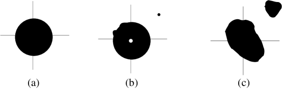
Figure 1: Droplets representing chiral primary states. In the field theory description these are droplets in phase space occupied by the fermions. In the gravity picture this is a particular two-plane in ten dimensions which specifies the solution uniquely. In (a) we see the droplet corresponding to the $AdS\times S$ ground state. In (b) we see ripples on the surface corresponding to gravitons in $AdS\times S$. The separated black region is a giant graviton brane which wraps an $S^{3}$ in $AdS_{5}$ and the hole at the center is a giant graviton brane wrapping an $S^{3}$ in $S^{5}$. In (c) we see a more general state.

The topology of the solutions is fixed by the topology of the droplets on the plane. The actual geometry depends on the shape of the droplets. In fact, this characterization is reminiscent of toric geometry. In the type IIB case we simply need to solve a Laplace equation. A circular droplet gives rise to the $AdS_{5}\times S^{5}$ solution, see figure 1. Small ripples on the droplet correspond to small fluctuations corresponding to gravitons in $AdS$. A small droplet far away from the circular one corresponds to a group of D3 branes wrapping an $S^{3}$ in $AdS_{5}$. A hole inside the circle corresponds to branes wrapping an $S^{3}$ in $S^{5}$. In the limit that the droplets become small these solutions reduce to the giant graviton branes that were discussed extensively in the literature [2, 3, 6]. Some of our solutions smoothly interpolate between branes wrapping the sphere and branes wrapping AdS. We can also have solutions that correspond to new geometries which cannot be thought of as branes. In other words, when we put many branes together they back-react on the geometry and we get new geometries with new topologies that are determined by geometric transitions. The transition is that the sphere the branes are wrapping becomes contractible while the transverse sphere becomes non-contractible and the branes get replaced by flux.

From the geometrical point of view we can consider this class of BPS geometries and we can wonder how we quantize them. Of course, the exact description in terms of fermions is telling us how to do it. In the type IIB case, a two dimensional plane contained in the ten dimensional geometry can be identified as the phase space of free fermions. The quantization of the area in the phase space amounts to the quantization of fluxes in the geometry. One interesting lesson is that geometries with very small topologically non-trivial fluctuations, or spacetime-foam, are already included when we perform the usual quantization of ordinary long wavelength gravitons.

These solutions are also interesting because they provide a relationship between free fermions and string theory which is rather different than the one we get from the $c=1$ matrix model (for reviews see [7]). Here the free fermions arise as the BPS sector of a ten dimensional string theory. Perhaps we should not be surprised because integrable systems often lead to free fermions and a BPS system is in some sense integrable, so it is natural to have a free fermion description. It would be nice to understand better whether there is a reduction of the usual superstring in AdS [8] to a string theory describing just this 1/2 BPS sector.

We can also describe 1/2 BPS excitations of the plane wave geometry, which corresponds to a half filled plane. In this case the fermion becomes a relativistic Dirac fermion in 1+1 dimensions. The light-cone energy of the solution is the same as the usual energy for a Dirac fermion. Particle-hole duality corresponds to exchanging the 3-sphere in the first four of the eight transverse coordinates with a 3-sphere in the last four coordinates.

By performing dualities we can get solutions which are dual to the mass deformed M2 brane theory [10, 11]. This theory is rather similar to the mass deformed $N=4$ Yang-Mills theory, or $N=1^{*}$ theory, analyzed by Polchinski and Strassler [12]. The mass term preserves $SO(4)\times SO(4)$ symmetry in $SO(8)$ and the theory has vacua that contain M5 branes wrapping an $S^{3}$ in the first four coordinates or an $S^{3}$ in the last four coordinates. Our solutions are non-singular and describe all possible vacua of this theory. By changing the fluxes on the various spheres, we can smoothly interpolate between the solutions with the M5 branes wrapping the first $S^{3}$ and the solutions with those wrapping the second $S^{3}$. This system has also been recently analyzed in [11], in terms of slightly different variables. Our approach leads to a simple way of constructing non-singular geometries.

We have also performed a similar analysis for the M-theory case, which corresponds to giant gravitons in $AdS_{4}\times S^{7}$ or $AdS_{7}\times S^{4}$. In this case we have similar droplets, and the 11 dimensional geometry is obtained after solving a three dimensional Toda equation. In this case we could only solve the equations explicitly in very simple examples. We also consider the M-theory plane wave. In this way we could find geometries that are dual to the BMN matrix model [13]. In particular, we find more evidence that the M5 brane emerges as a state of the BMN matrix model [14].

By performing a Wick rotation of the above analysis we are led to a characterization of all M-theory compactifications to $AdS_{5}$ that preserve ${\cal N}=2$ four dimensional supersymmetry. These are again given by solutions of the Toda equation but with slightly different boundary conditions. Indeed, we fit the previously known solutions [15] into this class. This constitutes an extension of the analysis in [19, 20] which characterized M-theory compactifications to $AdS_{5}$ preserving ${\cal N}=1$ four dimensional supersymmetry.

This paper is organized as follows. In section 2 we discuss the geometries associated to 1/2 BPS states in $AdS_{5}\times S^{5}$ or the type IIB pp-wave. In section 3 we discuss the 1/2 BPS geometries describing states in $AdS_{7}\times S^{4}$, $AdS_{4}\times S^{7}$, or M theory pp-wave. In various appendices we give more technical details.

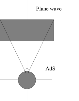
Figure 2: Plane wave configurations correspond to filling the lower half plane. This can be understood from the fact that the plane wave solution is a limit of the $AdS\times S$ solution.

2 1/2 BPS geometries in type IIB string theory

2.1 1/2 BPS states in the field theory

We consider ${\cal N}=4$ super Yang Mills on $S^{3}\times R$. We are interested in the class of states that preserves one half of the supersymmetries. These are the states associated to chiral primary operators that are built by taking products of traces of powers of a single chiral scalar field of $N=4$ Yang Mills. Denoting by $\phi^{i}$ the six scalars, we are interested in the field $Z=\phi^{1}+i\phi^{2}$, and the operators $\prod_{i}(TrZ^{n_{i}})^{r_{i}}$. These BPS states can be described in a variety of ways. The one that will be most useful for our purposes will be the description in terms of free fermions discussed in [4] (see also [21, 22]). These free fermions arise in the following way. We are interested in states with $\Delta-J=0$. The only such state is the lowest Kaluza-Klein mode of the field $Z$ on the $S^{3}$. This mode has a harmonic oscillator potential which arises from its conformal coupling to the curvature of $S^{3}$ [1]. So we are interested in the gauge invariant states of a matrix $Z$ in a harmonic oscillator potential. Standard arguments for matrix quantum mechanics [23] imply that the system reduces to $N$ fermions in a harmonic oscillator potential. We can think of these fermions as forming droplets in phase space. The ground state corresponds to a circular droplet. Equivalently, we can say that we have a quantum hall fluid. We can form the new Hamiltonian $H^{\prime}=H-J=\Delta-J$, where $J$ is the angular momentum in the 12 plane. In terms of this new Hamiltonian we have a Landau level problem. The 1/2 BPS states are the ground states of $H^{\prime}$ and correspond to the lowest Landau level. The AdS ground state corresponds to a circular droplet. The conformal dimension $\Delta=J$ of any excitation is given by the angular momentum on the Hall plane, or the energy of the harmonic oscillator, above the ground state corresponding to the circular droplet. It is also interesting to take the plane wave limit of these configurations. In terms of the droplets this amounts to zooming in on the edge of a droplet, as shown in figure 2. So the plane wave can be thought of as a Hall configuration where we fill the lower half plane ($x_{2}<0$). BPS excitations correspond to particles and/or hole excitations. These look like the states of a relativistic fermion. In fact, the lightcone energy of the states, $-p_{-}\sim J$, is indeed given by the expression of the energy for a relativistic fermion.

These BPS states preserve 16 non-trivial supersymmetries as well as $SO(4)\times SO(4)\times R$ bosonic symmetries, where $R$ corresponds to the Hamiltonian $H^{\prime}=H-J$. This generator commutes with the preserved supercharges.

2.2 1/2 BPS geometries in type IIB supergravity

We now look for the most general type IIB geometry that is invariant under $SO(4)\times SO(4)\times R$. This implies that the geometry will contain two three-spheres and a Killing vector. We only expect the five–form field strength to be excited. So we assume we have a geometry of the form

$$ds^{2} = g_{\mu\nu}dx^{\mu}dx^{\nu}+e^{H+G}d\Omega_{3}^{2}+e^{H-G}d{\tilde{\Omega}}_{3}^{2}$$ (2.1)

$$F_{(5)} = F_{\mu\nu}dx^{\mu}\wedge dx^{\nu}\wedge d\Omega_{3}+{\tilde{F}}_{\mu\nu}dx^{\mu}\wedge dx^{\nu}\wedge d{\tilde{\Omega}}_{3}$$ (2.2)

where $\mu,\nu=0,\cdots,3$. In addition, we assume that the dilaton and axion are constant and that the three-form field strengths are zero. The self duality condition on the five-form field strength implies that $F_{\mu\nu}$ and $\tilde{F}_{\mu\nu}$ are dual to each other in four dimensions:

$$F=e^{3G}*_{4}{\tilde{F}}~{},~{}~{}~{}~{}~{}F=dB,~{}~{}~{}~{}\tilde{F}=d\tilde{B}$$ (2.3)

We now demand that this geometry preserves the Killing spinor, i.e. we require that there are solutions to the equations

$$\nabla_{M}\eta+\frac{i}{480}\Gamma^{M_{1}M_{2}M_{3}M_{4}M_{5}}F^{(5)}_{M_{1}M_{2}M_{3}M_{4}M_{5}}\Gamma_{M}\eta=0$$ (2.4)

This equation is analyzed using techniques similar to the ones developed in [25, 19, 20]. One first writes the ten dimensional spinor as a product of four dimensional spinors and spinors on the spheres. Due to the spherical symmetry the problem reduces to a four dimensional problem involving a four dimensional spinor. One then constructs various forms by using spinor bilinears. These forms have interesting properties. For example, we can construct a Killing vector, which we assume to be non-zero. This is the translation generator, $\Delta-J$. There is another interesting form which is a closed one form. This can be used to define a local coordinate $y$. This coordinate $y$ is rather special since one can show that $y$ is the product of the radii of the two $S^{3}$s. By analyzing the Killing spinor equations one can relate the various functions appearing in the metric to a single function. This function ends up obeying a simple differential equation. We present the details of this analysis in appendix A. The end result is:

$$ds^{2} = -h^{-2}(dt+V_{i}dx^{i})^{2}+h^{2}(dy^{2}+dx^{i}dx^{i})+ye^{G}d\Omega_{3}^{2}+ye^{-G}d\tilde{\Omega}_{3}^{2}$$ (2.5)

$$h^{-2} = 2y\cosh G,$$ (2.6)

$$y\partial_{y}V_{i} = \epsilon_{ij}\partial_{j}z,\qquad y(\partial_{i}V_{j}-\partial_{j}V_{i})=\epsilon_{ij}\partial_{y}z$$ (2.7)

$$z = {1\over 2}\tanh G$$ (2.8)

$$F = dB_{t}\wedge(dt+V)+B_{t}dV+d\hat{B}~{},~{}~{}~{}~{}~{}~{}$$

$$\tilde{F} = d\tilde{B}_{t}\wedge(dt+V)+\tilde{B}_{t}dV+d\hat{\tilde{B}}$$ (2.9)

$$B_{t} = -{1\over 4}y^{2}e^{2G},~{}~{}~{}~{}~{}~{}~{}~{}~{}~{}~{}~{}~{}~{}~{}~{}~{}~{}~{}~{}~{}~{}~{}~{}~{}~{}\tilde{B}_{t}=-{1\over 4}y^{2}e^{-2G}$$ (2.10)

$$d\hat{B} = -{1\over 4}y^{3}*_{3}d({z+{1\over 2}\over y^{2}})~{},~{}~{}~{}~{}~{}~{}~{}~{}~{}~{}~{}~{}~{}~{}~{}~{}d\hat{\tilde{B}}=-{1\over 4}y^{3}*_{3}d({z-{1\over 2}\over y^{2}})~{}~{}$$ (2.11)

where $i=1,2$ and $*_{3}$ is the flat space epsilon symbol in the three dimensions parameterized by $y,x_{1},x_{2}$. We see that the full solution is determined in terms of a single function $z$. This function obeys the linear equation

$$\partial_{i}\partial_{i}z+y\partial_{y}({\partial_{y}z\over y})=0$$ (2.12)

Since the product of the radii of the two 3-spheres is $y$, we would have singularities at $y=0$ unless $z$ has a special behavior. It turns out that the solution is non-singular as long as $z=\pm{1\over 2}$ on the $y=0$ plane spanned by $x_{1},x_{2}$. Let us consider the case $z={1\over 2}$ at $y=0$. Then we see that $z$ will have an expansion $z\sim{1\over 2}-e^{-2G}={1\over 2}-y^{2}f(x)+\cdots$, where $f(x)$ will be positive with our boundary conditions. From this we find that $e^{-G}\sim yc(x)$. So we see that the metric in the $y$ direction and the second 3-sphere directions becomes

$$h^{2}dy^{2}+ye^{-G}d\tilde{\Omega}_{3}^{2}\sim{c(x)}(dy^{2}+y^{2}d\tilde{\Omega}_{3}^{2})$$ (2.13)

In addition we see that $h$ remains finite and the radius of the first sphere also remains finite. One can also show that $V$ remains finite by using the explicit expression we write below. When $z=-{1\over 2}$ the discussion is similar. In fact the transformation $z\to-z$ and an exchange of the two three–spheres is a symmetry of the equations. This corresponds to a particle hole transformation in the fermion system. This will not be a symmetry of the solutions if the fermion configuration itself is not particle-hole symmetric, or the asymptotic boundary conditions are not particle-hole symmetric (as in the $AdS_{5}\times S^{5}$ case). We will explain below that the solution is non-singular at the boundary of the two regions. So in order to determine the solution we need to specify regions in the $x_{1},x_{2}$ plane where $z=\pm{1\over 2}$. These two signs corresponds to the fermions and the holes, and the $x_{1},x_{2}$ plane corresponds to the phase space. After defining $\Phi=z/y^{2}$ the equation (2.12) becomes the Laplace equation in six dimensions for $\Phi$ with spherical symmetry in four of the dimensions, $y$ is then the radial variable in these four dimensions. The boundary values of $z$ on the $y=0$ plane are charge sources for this equation in six dimensions. It is then straightforward to write the general solution once we specify the boundary values. We find

$$z(x_{1},x_{2},y) = \frac{y^{2}}{\pi}\int_{\cal D}\frac{z(x_{1}^{\prime},x^{\prime}_{2},0)dx_{1}^{\prime}dx_{2}^{\prime}}{[({\bf x}-{\bf x}^{\prime})^{2}+y^{2}]^{2}}=-\frac{1}{2\pi}\int_{\partial{\cal D}}dl~{}n_{i}^{\prime}\frac{x_{i}-x_{i}^{\prime}}{[({\bf x}-{\bf x}^{\prime})^{2}+y^{2}]}+\sigma$$ (2.14)

$$V_{i}(x_{1},x_{2},y) = {\epsilon_{ij}\over\pi}\int_{\cal D}\frac{z(x_{1}^{\prime},x^{\prime}_{2},0)(x_{j}-x^{\prime}_{j})dx_{1}^{\prime}dx_{2}^{\prime}}{[({\bf x}-{\bf x}^{\prime})^{2}+y^{2}]^{2}}={\epsilon_{ij}\over 2\pi}\oint_{\partial{\cal D}}{dx^{\prime}_{j}\over({\bf x}-{\bf x}^{\prime})^{2}+y^{2}}$$ (2.15)

where in the second expressions for $z,V_{i}$ we have used that $z(x_{1}^{\prime},x_{2}^{\prime},0)$ is locally constant and we have integrated by parts to convert integrals over droplets ${\cal D}$ into the integrals over the boundary of the droplets $\partial{\cal D}$. In these expressions $n_{i}$ is the unit normal vector to the droplet pointing towards the $z={1\over 2}$ regions, $\sigma$ is a contribution from infinity which arises in the case that $z$ is constant outside a circle of very large radius (asymptotically $AdS_{5}\times S^{5}$ geometries). $\sigma=\pm{1\over 2}$ when we have $z=\pm{1\over 2}$ asymptotically. The contour integral in (2.15) is oriented in such a way that the $z=-{1\over 2}$ region is to the left. We see from the second expression for $V$ in (2.15) that $V$ is finite as $y\to 0$ in the interior of a droplet. We also see from (2.15) that $V$ is a globally well defined vector field. This is important since we want the time direction parameterized by $t$ to be well defined (i.e. we do not want NUT charge).

2.3 Examples

Let us now consider a simple solution which is associated to the half filled plane. We have the boundary conditions

$$z(x_{1}^{\prime},x_{2}^{\prime},0)=\frac{1}{2}\mbox{sign}~{}x^{\prime}_{2}$$ (2.16)

From this data we can compute the entire function $z(x_{2},y)$ using (2.14), (2.15)

$$z(x_{2},y) = \frac{1}{2}\frac{x_{2}}{\sqrt{x_{2}^{2}+y^{2}}}$$ (2.17)

$$V_{1} = {1\over 2}{1\over\sqrt{x_{2}^{2}+y^{2}}}~{},~{}~{}~{}~{}~{}~{}V_{2}=0$$ (2.18)

Inserting this into the general ansatz (2.5) and performing the change of coordinates

$$y = r_{1}r_{2}$$ (2.19)

$$x_{2} = {1\over 2}(r_{1}^{2}-r_{2}^{2})$$ (2.20)

we obtain the usual form of the metric for the plane wave [24]

$$ds^{2}=-2dtdx_{1}-(r^{2}_{1}+r_{2}^{2})dt^{2}+d{\vec{r}}_{1}^{\,2}+d{\vec{r}}_{2}^{\,2}$$ (2.21)

We see that the final solution is smooth, despite the fact that on the $y=0$ plane $V$ diverges at the boundary between two regions ($x_{2}=0$ in this case). In fact, this computation shows that, in general, the boundary between two regions is smooth. The reason is that locally the boundary between two regions looks like the plane wave and therefore we will get a non-singular metric.

Let us now recover the familiar $AdS_{5}\times S^{5}$ geometry. In this case it is convenient to introduce a function $\tilde{z}=z-{1\over 2}$. The Laplace equation for $\tilde{z}/y^{2}$ has sources on a disk of radius $r_{0}$. We choose polar coordinates $r,\phi$ in the $x_{1},x_{2}$ plane. We obtain

$${\tilde{z}}(r,y) = -\frac{y^{2}}{\pi}\int_{\rm Disk}\frac{r^{\prime}dr^{\prime}d\phi}{[r^{2}+r^{\prime 2}-2rr^{\prime}\cos\phi+y^{2}]^{2}}$$

$${\tilde{z}}(r,y;r_{0}) \equiv \left.\frac{r^{2}-r_{0}^{2}+y^{2}}{2\sqrt{(r^{2}+r_{0}^{2}+y^{2})^{2}-4r^{2}r_{0}^{2}}}\right.-{1\over 2}$$ (2.22)

$$V_{\phi} = -r\sin\phi V_{1}+r\cos\phi V_{2}=-\frac{1}{2\pi}\int_{\partial{\cal D}}\frac{rr^{\prime}\cos\phi^{\prime}d\phi^{\prime}}{r^{2}+r^{\prime 2}+y^{2}-2rr^{\prime}\cos\phi^{\prime}}$$

$$V_{\phi}(r,y;r_{0}) \equiv -\frac{1}{2}\left.\left(\frac{r^{2}+y^{2}+r_{0}^{2}}{\sqrt{(r^{2}+r_{0}^{2}+y^{2})^{2}-4r^{2}r_{0}^{2}}}-1\right)\right.$$ (2.23)

Inserting this into the general ansatz and performing the change of coordinates

$$y = r_{0}\sinh\rho\sin\theta$$ (2.24)

$$r = r_{0}\cosh\rho\cos\theta$$ (2.25)

$$\tilde{\phi} = \phi-t$$ (2.26)

we see that we get the standard $AdS_{5}\times S^{5}$ metric

$$ds^{2}=r_{0}[-\cosh^{2}\rho dt^{2}+d\rho^{2}+\sinh^{2}\rho d\Omega_{3}^{2}+d\theta^{2}+\cos^{2}\theta d\tilde{\phi}^{2}+\sin^{2}\theta d\tilde{\Omega}_{3}^{2}]$$ (2.27)

So we see that $r_{0}=R^{2}_{AdS}=R_{S^{5}}^{2}$. In fact, under an overall scaling of the coordinates $(x_{i},y)\to\lambda(x_{i},y)$ the metric scales by a factor $\lambda$. This is what we expect since the total area of the droplets is equal to the number of branes, a fact which we will demonstrate later. By comparing the value of the $AdS$ radius we obtained in (2.27) and the standard answer, $R^{4}_{AdS}=4\pi l_{p}^{4}N$, we can write the precise quantization condition on the area of the droplets in the 12 plane as

$$({\rm Area})=4\pi^{2}l_{p}^{4}N~{},~{}~{}~{}~{}~{}~{}~{}~{}~{}~{}~{}{\rm or}~{}~{}~{}\hbar=2\pi l_{p}^{4}$$ (2.28)

where $N$ is an integer, and we have defined an effective $\hbar$ in the $x_{1},x_{2}$ plane, where we think of the $x_{1},x_{2}$ plane as phase space.

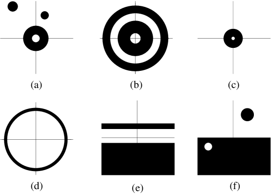
Figure 3: We see various configurations whose solutions can be easily constructed as superpositions of the $AdS_{5}\times S^{5}$ solution and the plane wave solution. In (a) we see an example of the type of configurations that can be obtained by superimposing the circular solution (2.22). In (b) we see generic configurations that lead to solutions which have two Killing vectors and lead to static configurations in $AdS$. In (c) we see the solution corresponding to a superposition of D3 branes wrapping the $\tilde{S}^{3}$ in $S^{5}$. In (d) we see the configuration resulting from many such branes, which can be thought of as a superposition of branes on the $S^{3}$ of $AdS_{5}$ uniformly distributed along the angular coordinate $\tilde{\phi}$ of $S^{5}$. In (e) we see a configuration that can be viewed as an excitation of a plane wave with constant energy density. In (f) we see a plane wave excitation with finite energy.

Now that we have constructed the solution for a circular droplet, we can construct in a trivial way the solutions that are superpositions of circles, see figure 3(a) . Among these the ones corresponding to concentric circles have an extra Killing vector. These lead to time independent configurations in $AdS$. All other solutions will depend on $\phi=t+\tilde{\phi}$ where $t$ is the time in $AdS$ and $\tilde{\phi}$ is an angle on the asymptotic $S^{5}$, see (2.27). The solutions corresponding to concentric circles are therefore superpositions of (2.22) and (2.23)

$$\tilde{z}=\sum_{i}(-1)^{i+1}\tilde{z}(r,y;r^{(i)}_{0}),\qquad V_{\phi}=\sum_{i}(-1)^{i+1}V_{\phi}(r,y;r^{(i)}_{0})$$ (2.29)

Here $r_{0}^{(1)}$ is the radius of the outermost circle, $r_{0}^{(2)}$ the next one, etc (see figure 3(b)). Let us discuss the solution corresponding to a single black ring 3(c). When the white hole in the center is very small, this can be viewed as branes wrapping a maximal $\tilde{S}^{3}$ in $S^{5}$. When the area of this hole, $N_{h}$, is smaller than the original area, $N$, of the droplet ($N_{h}\ll N$), the solution will locally look like an $AdS_{5}\times S^{5}$ solution near the hole. When we increase the number of branes wrapped on $\tilde{S}^{3}$ in $S^{5}$ the area of the holes becomes very large and in the limit we get a rather thin ring, which could be viewed as a superposition of D3 branes wrapping an $S^{3}$ in $AdS_{5}$ , see figure 3(d).

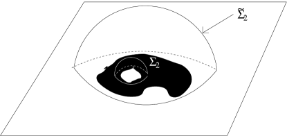
Figure 4: We can construct a five-manifold by adding the sphere $\tilde{S}^{3}$ fibered over the surface $\tilde{\Sigma}_{2}$. This is a smooth manifold since at the boundary of $\tilde{\Sigma}_{2}$ on the $y=0$ plane the sphere $\tilde{S}^{3}$ is shrinking to zero. The flux of $F_{5}$ is proportional to the area of the black region inside $\tilde{\Sigma}_{2}$. Another five manifold can be constructed by taking $\Sigma_{2}$ and adding the other three–sphere $S^{3}$. The flux is proportional to the area of the white region contained inside $\Sigma_{2}$.

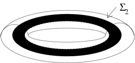
Figure 5: We see here an example of a two dimensional surface, $\Sigma_{2}$, that is surrounding a ring. If we add the three–sphere $\tilde{S}^{3}$ fibered over $\Sigma_{2}$ we get a five manifold with the topology of $S^{4}\times S^{1}$.

2.4 Topology and charges of the solutions.

Let us explore the topology of the solutions. This analysis is somewhat similar to that used in toric geometry. As long as $y\not=0$ we have two $S^{3}$s. Let us denote these two spheres as $S_{3}$ and $\tilde{S}_{3}$. At the $y=0$ plane the first sphere shrinks in a non-singular fashion if $z=-\frac{1}{2}$ while the second sphere, $\tilde{S}^{3}$, shrinks if $z=\frac{1}{2}$. Both spheres shrink at the boundary of the two regions. In fact there is a shrinking $S^{7}$ at these points, since the geometry is locally the same as that of a pp-wave. For example, in the $AdS_{5}\times S^{5}$ solution the second sphere, $\tilde{S}_{3}$, shrinks at $y=0$ outside the circle, this is the three–sphere contained in $S^{5}$. On the other hand the three–sphere contained in $AdS_{5}$ shrinks at $y=0$ inside the circular droplet. Consider a surface $\tilde{\Sigma}_{2}$ on the $(y,\vec{x})$ space that ends at $y=0$ on a closed, non-intersecting curve lying in a region with $z=\frac{1}{2}$ see figure 4 . We can construct a smooth five dimensional manifold by fibering the second three sphere, $\tilde{S}^{3}$, on $\tilde{\Sigma}_{2}$. This is a smooth manifold which is topologically a five–sphere. We can now measure the flux of the five-form field strength $F_{5}$ on this five-sphere. Looking at the expressions for the field strength (2.2) in terms of the four dimensional gauge field (2.11), (2.9) we find that the spatial components are given by $\tilde{F}|_{spatial}=d(\tilde{B}_{t}V)+d\hat{\tilde{B}}$. Since $B_{t}V$ is a globally well defined vector field the flux is given by

$$\tilde{N}=-{1\over 2\pi^{2}l_{p}^{4}}\int d\hat{\tilde{B}}={1\over 8\pi^{2}l_{p}^{4}}\int_{\tilde{\Sigma}_{2}}y^{3}*_{3}d\left({z-{1\over 2}\over y^{2}}\right)={({\rm Area})_{z=-{1\over 2}}\over 4\pi^{2}l_{p}^{4}}$$ (2.30)

where $\tilde{\Sigma}_{2}$ is the two surface in the three dimensional space spanned by $y,x_{1},x_{2}$. This expression gives the total charge inside this region for the Laplace equation, which in turn is equal to the total area with $z=-{1\over 2}$ contained within the contour on which $\tilde{\Sigma}_{2}$ ends at $y=0$, see figure 4. Note that (2.30) leads to the quantization of area, (2.28). In the $AdS_{5}\times S^{5}$ case there is only one non-trivial five–sphere and this integral gives the total flux. This flux is quantized in the quantum theory.

We can consider an alternative five–sphere by considering a surface that ends on the $y=0$ plane on a region with $z=-\frac{1}{2}$ (see figure 4). The flux over this five–manifold is given by

$$N={1\over 2\pi^{2}l_{p}^{4}}\int d\hat{B}=-{1\over 8\pi^{2}l_{p}^{4}}\int_{\Sigma_{2}}y^{3}*_{3}d\left({z+{1\over 2}\over y^{2}}\right)={({\rm Area})_{z={1\over 2}}\over 4\pi^{2}l_{p}^{4}}$$ (2.31)

and it measures the total area of the other type, with $z=\frac{1}{2}$, contained in this region. If these fluxes are non-zero, then these spheres are not contractible. So if we have a large number of droplets, we have a complicated topology for the solution. In addition we can construct other 5-manifolds which are not five–spheres by considering more complicated surfaces. For example we get the five-manifold with topology $S^{4}\times S^{1}$ from the surface depicted in figure 5.

Another interesting property of the solutions is their energy or their angular momentum $J$. These are equal to each other due to the BPS condition $\Delta=J$. As explained in [4], this energy is the energy of the fermions in a harmonic oscillator potential minus the energy of the ground state of $N$ fermions. From the gravity solution it is easier to read off the angular momentum. This involves computing the leading terms in the $g_{\phi+t,t}$ components of the metric. The details of this computation are given in appendix E. The final expression is

$$\Delta = J={1\over 16\pi^{3}l_{p}^{8}}\left[\int_{\cal D}d^{2}x(x_{1}^{2}+x_{2}^{2})-{1\over 2\pi}\left(\int_{\cal D}d^{2}x\right)^{2}\right]$$ (2.32)

$$= \int_{\cal D}{d^{2}x\over 2\pi\hbar}{{1\over 2}(x_{1}^{2}+x_{2}^{2})\over\hbar}-{1\over 2}\left(\int_{\cal D}{d^{2}x\over 2\pi\hbar}\right)^{2}$$

where $\cal D$ is the domain where $z=-{1\over 2}$, which is the domain where the fermions are. Using the definition of $\hbar$ in (2.28) we see that this is the quantum energy of the fermions minus the energy of the ground state.

None of the solutions described here has a horizon and they are all regular solutions. A singular solution was considered in [28]. That solution was obtained as the extremal limit of a charged black hole in gauged supergravity [29, 30]. Since it is a BPS solution it obeys our equations. We find that the boundary conditions on the $y=0$ plane are such that we have a disk, similar to the one we have in $AdS$ but the boundary value of $2z$ is not $-1$ but $-1/(1+q)$ where $q$ is the charge parameter of the singular solution. Of course, the solution is singular because it violates our boundary condition, but it could be viewed as an approximation to the situation where we dilute the fermions, or we consider a uniform gas of holes in the disk, which agrees with the picture in [28].

Figure 6: In (a) we see a small circular droplet of area $\hbar$ that is at some distance $d$ from a bigger droplet which is described by a smooth gravity solution. If the distance $d$ is larger than $\sqrt{\hbar}$ this is a topologically non-trivial excitation with an energy of the order of $M_{pl}$ above the ground state. As $d\to 0$ the energy decreases, but its curvature increases and, in the fermion picture, such an excitation is better described in terms of ripples of the Fermi surface, as in (b). These are gravitons propagating in the smooth original geometry. Notice that the geometries corresponding to pictures (a) and (b) have different topologies.

Note that any droplet which is far away from other droplets will look locally near the droplet like $AdS_{5}\times S^{5}$. In particular if we have a fermion droplet with $z=-{1\over 2}$ surrounded by a sufficiently large region with $z={1\over 2}$, then in the $z={1\over 2}$ region we see that $S^{3}$ is not contractible. The droplet can be viewed as branes wrapped on $S^{3}$. On the droplet itself, the $S^{3}$ is contractible but now there is a new $S^{5}$ that is not contractible, so we have a geometric transition. The $S^{5}$ is constructed by fibering the three–sphere $\tilde{S}^{3}$ on a surface $\tilde{\Sigma}_{2}$ which surrounds the droplet as in figure 4. If the amount of flux is small, these geometries can be viewed as branes in an background geometry, but as the flux becomes large they can be viewed as smooth geometries with fluxes. Note that even a single brane, can be viewed as a highly curved smooth geometry with flux, but this geometrical description is misleading for some aspects of the physics. In fact we expect that curvatures will become high if the dimensions of the droplets become of order one. More precisely, we expect that curvatures will become high if the linear dimensions of the droplet become of order $\sqrt{\hbar}$, or if two droplets come close together at distances smaller than $\sqrt{\hbar}$. Note that if we have a small circular droplet of area $\hbar$ and we bring it to within a distance of order $\sqrt{\hbar}$ from the big circular droplet corresponding to the $AdS$ ground state, then the configuration has an energy of order $M_{pl}$ in ten dimensions. If we bring this small droplet to a distance $d\ll\sqrt{\hbar}$ from the big circular droplet we will get a highly curved geometry that formally has very small energy. On the other hand low energy excitations described by gravity modes correspond to small long wavelength fluctuations of the big circular droplet. It is clear from the fermion picture that a fermion very close to the Fermi surface is well described by the boson characterizing long wavelength excitations of the fermion fluid. So we conclude that highly curved topologically non-trivial excitations with very small energies are already included as gravity modes, see figure 6. Here we have always discussed the curvature of the solution in Planck units. If the string coupling is small, the geometry can be rendered invalid by stringy corrections at a smaller curvature scale.

The solutions we are discussing here are somewhat reminiscent of the Coulomb branch solutions that arise when we consider $D3$ branes on $R^{1+3}$. In fact, the $SO(4)$ invariant subset of the latter can be obtained from the solutions in this paper by taking appropriate limits (see appendix B).

Distributions of droplets in a compact region of the 12 plane lead to solutions with $AdS_{5}\times S^{5}$ asymptotics. Solutions which correspond to finite deformations of the half filled plane are asymptotic to the pp-wave geometry. Let us discuss the latter solutions a bit more. Solutions with a small droplet or a small hole, see figure 3 (f), correspond to branes wrapping the $S^{3}$ or $\tilde{S}^{3}$. Large size droplets correspond to new geometries with fluxes. One can also consider solutions that are translation invariant along $x_{1}$. These are solutions corresponding to empty and occupied bands see figure 3 (e). These solutions have infinite energy, but finite energy density. We can also compactify the direction $x_{1}$. This is really a DLCQ compactification, since the solution asymptotes to a pp-wave where $x_{1}=x^{-}$, see (2.21). These solutions correspond to the DLCQ of the pp-wave. The momentum $-p_{-}$ is the energy of the fermion configuration after we take the Fermi surface to be in a position such that the total number of particles and holes is the same.

2.5 M2 brane theory with a mass deformation

In this section we consider geometries that are dual to the M2 brane theory with a mass deformation [31, 11]. Starting with the usual theory on coincident M2 branes, it is possible to introduce a mass deformation that preserves 16 supercharges. This deformation preserves an $SO(4)\times SO(4)$ subgroup of the $SO(8)$ R-symmetry group of the conformal M2 brane theory. One interesting aspect of this theory is that its features are rather similar to those of ${\cal N}=4$ SYM with a mass deformation. Namely, the mass deformed M2 brane theory also has vacua that are given by dielectric branes [32]. In this case these are M5 branes that are wrapping a 3-sphere in the first four of the eight transverse coordinates or a 3-sphere in the last four of the eight transverse coordinates. We can obtain these solutions by U-dualizing some of the solutions discussed above. The authors of [11] managed to reduce the problem to finding a solution of a harmonic equation. The relation between their function and ours is given in appendix C. Our parametrization of the ansatz has the advantage that it is very simple to select out the non-singular solutions.

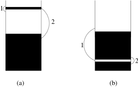
Figure 7: We see the configurations corresponding to two of the vacua of the mass deformed M2 brane theory. The vacuum in (a) can be viewed as dielectric M5 branes wrapping the $S^{3}$ in the first four coordinates of the eight transverse coordinates. The configuration in (b) corresponds to a vacuum with M5 branes wrapping the $S^{3}$ in the second four coordinates. The two geometries have the same topology. Consider arcs in the $x_{2},y$ plane that enclose the fermions or the holes and end at $y=0$. We can construct four spheres by taking one of these arcs and tensoring the $S^{3}$ that shrinks to zero at the tip of the arcs. The two different $S^{3}$ are denoted in the figure by indices $1$ and $2$. The flux of $F_{4}$ over these four spheres is equal to the number of particles or holes enclosed by the arcs. Note that the horizontal line in this figure does not correspond to a coordinate in the final M-theory geometry.

This system is intimately related to the type IIB solutions that we considered above. One way to see the connection is the following. It was argued in [33] that the DLCQ of type IIB string theory with $N$ units of DLCQ momentum is the same as the theory on $N$ M2 branes on a torus. We can now consider the DLCQ of the maximally supersymmetric pp-wave, where we periodically identify along the lightlike Killing direction, $x^{-}\sim x^{-}+2\pi R$ in (2.21). The sector with $N$ units of momentum $-p_{-}=N/R$ is given by the mass deformed M2 brane theory on a torus . From the pp-wave point of view it is clear that there can be supersymmetric vacua that correspond to D3 branes wrapping either of the $S^{3}$s. On the M-theory side, these map into vacua of the M2 brane theory where the M2 branes form an M5 brane wrapping either of the two $S^{3}$s. There is a large number of vacua that are in one to one correspondence with the partitions of $N$. Perhaps the simplest way to count these vacua is to recall yet another description of this DLCQ theory in terms of a limit of a gauge theory in [35]. According to the description in [35] the vacua are given in terms of chiral primary operators of a particular large $N$ limit of an orbifold theory. It is a simple matter to count those and notice that they are equivalent to partitions of $N$. This is of course related in a simple manner to the fermion fluid picture for the pp wave. Once we compactify $x^{-}$ we have fermions on a cylinder, where we fill half the cylinder. The asymptotic conditions automatically imply that we are only interested in states with zero $U(1)$ charge. The $U(1)$ charge is related to the position of the Fermi level. We always choose it such that the total number of particles and holes is zero. The energy of the fermions is the same as the number $N$ of M2 branes. These are relativistic fermions which can be bosonized and the number of states with energy $E=N$ is indeed given by the partitions of $N$. States which contain highly energetic holes or particles, as shown in figure 7, correspond to M5 branes wrapping one or the other $S^{3}$. Configurations in between are better thought of as smooth geometries with fluxes. An interesting fact is that the geometry corresponding to a highly energetic fermion, as in figure 7(a), and the geometry corresponding to a highly energetic hole, as in figure 7 (b), are topologically the same. The reason is that the geometry contains two distinct $S^{4}$s through which we have a non-vanishing flux. Consider for example the configuration in figure 7 (a), which can be interpreted as M5 branes wrapping one of the $S^{3}$s. One $S^{4}$ is the obvious one that is transverse to these branes. The other $S^{4}$ arises in an interesting way. Consider the three–sphere that these branes are wrapping. At the center of the space, where one normally imagines the $M2$ branes, this three–sphere is contractible. As we start going radially outwards we encounter the M5 branes, the backreaction of the branes on the geometry will make the $S^{3}$ on their worldvolumes contractible. So the end result is that the $S^{3}$ contracts to zero on both end points of the interval that goes between the origin and the branes. This produces another $S^{4}$. Through this $S^{4}$ we have a large flux, which we might choose to view as part of the background flux, the flux that was there before we put in the M2 branes, the flux which is responsible for the mass term on the M2 brane theory. A configuration with highly energetic holes corresponds to M5 branes wrapping the second $S^{3}$. This is topologically the same as the configuration with highly energetic fermions. In other words, the two configurations in figure 7 have the same topology. They only differ in the amount of four form flux over the two $S^{4}$s.

In this problem there is a precise duality under the interchange of the two three–spheres, which maps solutions into each other. Some special solutions will be invariant under the duality. This is particle hole duality in the fermion picture.

Finally, let us give the explicit form of the solutions

$$ds^{2}_{11} = e^{4\Phi\over 3}(-dt^{2}+dw_{1}^{2}+dw_{2}^{2})$$ (2.33)

$$~{}~{}~{}~{}~{}~{}~{}~{}~{}~{}+e^{-2\Phi\over 3}\left[h^{2}(dy^{2}+dx_{2}^{2})+ye^{G}d\Omega_{3}^{2}+ye^{-G}d\tilde{\Omega}_{3}^{2}\right]$$

$$e^{2\Phi} = {1\over h^{2}-h^{-2}V_{1}^{2}}$$ (2.34)

$$F_{4} = -d(e^{2\Phi}h^{-2}V_{1})\wedge dt\wedge dw_{1}\wedge dw_{2}$$ (2.35)

$$~{}~{}~{}~{}~{}~{}~{}~{}~{}~{}-{1\over 4}e^{-2\Phi}[e^{-3G}*_{2}d(y^{2}e^{2G})\wedge d\tilde{\Omega}_{3}+e^{3G}*_{2}d(y^{2}e^{-2G})\wedge d\Omega_{3}]$$

where $*_{2}$ is the flat epsilon symbol in the coordinates $y,x_{2}$ and $h,G$ are given by the expressions we had above (2.6)–(2.8), (2.12). These functions are determined by considering boundary conditions corresponding to strips that are translation invariant along $x_{1}$, see figure 3(e) and equations (2.17), (2.18). Note that since we had translation symmetry along $x_{1}$ in the original IIB solution, only the component $V_{1}$ is nonzero. The coordinate $x_{1}$ does not appear in this M-theory solution because it was U-dualized. So $z$, $V_{1}$ are given by superpositions of solutions of the form (2.17)–(2.18). In other words

$$z(x_{2},y)=\sum_{i}(-1)^{i+1}z^{pp}(x_{2}-x_{2}^{i},y),\qquad V_{1}(x_{2},y)=\sum_{i}(-1)^{i+1}V_{1}^{pp}(x_{2}-x_{2}^{i},y)$$ (2.36)

where $z^{pp},V_{1}^{pp}$ are the functions in (2.17), (2.18), and $x_{2}^{i}$ is the position of the $i$th boundary starting from the bottom of the Fermi sea. The relation between our parametrization of the solution, (2.33)-(2.35), and the parametrization in [11] is given in appendix C.

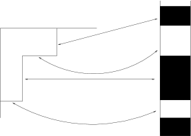
Figure 8: Correspondence between the Young diagrams and the states of free fermions. We start from the bottom left of the Young diagram, each time we move right by $n$ boxes we add $n$ holes and each time we move up by $n$ boxes we add $n$ fermions. The energy of the configuration is equal to the total number of boxes of the Young diagram.

These solutions can be related to Young diagrams in a simple way which is pictorially represented in figure 8. We start at the bottom of the Young diagram and we move along the boundary. Each time we move up we add as many fermions as boxes, each time we move right we add holes. The Fermi level is set so that the total number of holes is equal to the total number of fermions. Then the energy of the fermion system is equal to the number of boxes, and in our case this is the number of M2 branes. Of course, small curvature solutions are only those where the Young diagram has a small number of corners and a large number of boxes. This is in contrast to the situation encountered in other cases [37, 38] where smooth Young diagrams correspond to smooth macroscopic configurations. In our case, a Young diagram which contains edges separated by few boxes leads to solutions with Planck scale curvature.

Using Young diagrams we can describe in a similar way the circularly symmetric configurations in the $x_{1},x_{2}$ plane. Solutions that are not circularly symmetric are given by superpositions of these diagrams. In other words, the Young diagrams are in direct correspondence with the momentum basis for the fermions. Generic states that are not invariant under translations (or rotations) are given, in the Hilbert space, by a superposition of these. In the gravity description the only states that lead to smooth geometries are those which form well defined droplets in the Fermi sea.

Figure 9: We see fermion configurations corresponding to a single isolated strip, or set of strips. These fermions are the same as the ones that appear in 2d QCD on a cylinder, or $SU(N)$ group quantum mechanics. In (a) we display the ground state and in (b) we display an excited state. From the point of view of D4 brane on $S^{3}\times S^{1}\times R$ these are all supersymmetric ground states.

It is also interesting to consider fermion distributions that are not asymptotic to the distributions for $AdS\times S$ or plane waves. For example, we can consider a single isolated strip of fermions, as in figure 9. If we compactify the $x_{1}$ coordinate then the fermion configuration is the same as the one we have in two dimensional QCD on a cylinder. In fact, the dual field theory configuration for a single isolated strip (or single collection of strips) is $N$ M-fivebranes wrapped on $S^{3}\times T^{2}\times R$, where $N$ is given by the area of the strip. We can also think of this as Yang Mills theory on $S^{3}\times S^{1}\times R$. The reduction on $S^{3}$ leaves us with a gauge theory in two dimensions, which has BPS vacua that are in correspondence with the states of 2d Yang-Mills theory on a circle [39]. We discuss this a bit more in appendix D. There are other asymptotic configurations that could be explored, such as wedges in the $12$ plane, etc.

In the ${\cal N}=1^{*}$ theory considered in [12] we expect a similar situation, where geometries will be non-singular but could have large curvatures when some of the fluxes become small.

2.6 Analytic continuation to $AdS_{3}\times S^{3}\times S^{1}$

If we want to describe solutions with $AdS_{3}\times S^{3}$ factors, rather than $S^{3}\times S^{3}$, then the following minor changes should be made from (2.5)-(2.9):

$$y=iy^{\prime}~{},~{}~{}~{}~{}~{}~{}~{}~{}G=G^{\prime}+{i\pi\over 2}~{},~{}~{}~{}~{}~{}~{}~{}~{}x_{j}=ix^{\prime}_{j}$$ (2.37)

$$d\Omega_{3}^{2}=-ds^{2}_{AdS_{3}}$$ (2.38)

Then we find that

$$h^{-2}=-y^{\prime}(e^{G^{\prime}}-e^{-G^{\prime}})~{},~{}~{}~{}~{}~{}V_{j}=-iV_{j}^{\prime},~{}~{}~{}~{}~{}z={1\over 2\tanh G^{\prime}}$$ (2.39)

After we insert these expressions in the ansatz (2.5)-(2.9) and we take all primed quantities to be real we get a real solution with an $AdS_{3}\times S^{3}$ factors. The coordinate parameterized by $t$ is now spacelike, so we can take it to be compact. We can set $t=\chi$ . It would be nice to see if there are any solutions with a compact internal manifold. Of course we have the well known $AdS_{3}\times S^{3}\times T^{4}$ or $AdS_{3}\times S^{3}\times K3$ solutions. But our ansatz does not cover these, because in our case the $\chi$ translation generator appears in the right hand side of the supersymmetry algebra (as a $U(1)$ central charge). We did not manage to find any solutions with a compact internal manifold.

We find an interesting limit of these analytically continued solutions, under which the $AdS_{3}\times S^{3}$ factor becomes a 6-dimensional flat space and the remaining 4-dimensional transverse space turns out to be a Hyper-Kahler manifold with a translational Killing vector [41]. Let us look for a solution of the equation,

$$\partial_{i^{\prime}}\partial_{i^{\prime}}z+y^{\prime}\partial_{y^{\prime}}({1\over y^{\prime}}\partial_{y^{\prime}}z)=0$$ (2.40)

We will consider the solution in the range $|y^{\prime}-y_{0}|\ll y_{0}$ and rewrite $z$ as $z\sim y_{0}g$, then $g$ satisfies the 3d Laplace equation

$$\partial_{i^{\prime}}\partial_{i^{\prime}}g+\partial_{y^{\prime}}^{2}g=0$$ (2.41)

We could consider solutions where $g$ is asymptotically a constant if wanted. We will now take the limit $y_{0}\to\infty$ and $z\to\infty$ and from (2.39) we see

$$z\sim{1\over 2G^{\prime}},~{}~{}~{}~{}~{}~{}~{}h^{-2}\sim-y_{0}2G^{\prime}\sim-{1\over g}$$ (2.42)

We now insert this and (2.39) into the general ansatz (2.5) for the ten dimensional metric. We find that the radii of $AdS_{3}\times S^{3}$ go to infinity and we recover six dimensional flat space. The remaining four dimensional manifold becomes

$$ds_{4}^{2} = {1\over g}(d\chi+V^{\prime}_{i}dx^{\prime i})^{2}+g(dy^{\prime 2}+dx^{\prime i}dx^{\prime i})$$ (2.43)

$$dV^{\prime} = {1\over y^{\prime}}*_{3}dz\sim*_{3}dg$$ (2.44)

This is a metric of the Gibbons-Hawking form, which is the general form for a 4d hyper-Kahler manifold with one translational Killing vector [41] (see also [16, 17]). In particular note that $y_{0}$ scales out of the definition of $V^{\prime}$ in (2.44). In order to have interesting solutions we should allow delta functions in the right hand side of (2.41) with appropriate coefficients.

3 1/2 BPS geometries in M-theory

In this section we perform an analogous analysis for M-theory solutions associated to 1/2 BPS geometries in $AdS_{4,7}\times S^{7,4}$. We first describe how to reduce the problem to the Toda equation. We then discuss some interesting dualities and Wick rotations.

Let us consider 1/2 BPS geometries in $AdS_{7}\times S^{4}$. These are associated to the chiral primaries of the $(0,2)$ theory. The chiral primaries of the $(0,2)$ theory can also be described in terms of Young diagrams with at most $N$ rows [36], as in four dimensional ${\cal N}=4$ SYM. So in terms of labeling of states we also have free fermions on a plane. We expect a similar picture if we study chiral primaries of the 2+1 superconformal field theory related to $AdS_{4}\times S^{7}$.

These states preserve 16 supercharges which transform under $SO(3)\times SO(6)\times R$. In this case we expect that the $R$ translation generator does not leave the spinor invariant, rather the spinor has non-zero energy under this generator. This $R$ generator should leave the geometries invariant.

We look for supersymmetric solutions of 11D supergravity which have $SO(6)\times SO(3)$ symmetry

$$ds_{11}^{2} = e^{2\lambda}\left(4d\Omega_{5}^{2}+e^{2A}d{\tilde{\Omega}}_{2}^{2}+ds_{4}^{2}\right)$$ (3.1)

$$G_{(4)} = G_{\mu_{1}\mu_{2}\mu_{3}\mu_{4}}dx^{\mu_{1}}\wedge dx^{\mu_{2}}\wedge dx^{\mu_{3}}\wedge dx^{\mu_{4}}+F_{\mu_{1}\mu_{2}}dx^{\mu_{1}}\wedge dx^{\mu_{2}}\wedge d^{2}{\tilde{\Omega}}$$ (3.2)

where $d\Omega_{5}^{2}$ and $d{\tilde{\Omega}}_{2}^{2}$ are the metrics on unit radius spheres and $\mu_{i}=0,\cdots,3$. Using the equations for the field strength, one can show that

$$G_{\mu_{1}\mu_{2}\mu_{3}\mu_{4}}=I_{1}e^{-3\lambda-2A}\epsilon_{\mu_{1}\mu_{2}\mu_{3}\mu_{4}}$$ (3.3)

with constant $I_{1}$. In the solutions related to chiral primaries on $AdS\times S$ or pp-waves the $S^{2}$ or the $S^{5}$ can shrink, at least in the asymptotic regions. These spheres cannot shrink in a non-singular manner if the flux $I_{1}$ were non-vanishing. The reason is that the flux density would diverge at the points where the spheres shrink. So from now on we set $I_{1}=0$. In order to continue constraining the metric we decompose the Killing spinor in terms of a four dimensional Killing spinor and spinors on $S^{2}$ and $S^{5}$. So we have an effective problem in four dimensions with a four dimensional gauge field $B_{\mu}$ and two scalars $A,\lambda$. A closely related problem was analyzed in [19], where general supersymmetric M-theory solutions with $SO(2,4)\times U(1)$ symmetry were considered. Our solutions preserve more supersymmetries, but after a suitable Wick rotation they are particular examples of the general situation considered in [19] so we can use some of their methods. After a rather long analysis, which can be found in appendix F, the end result is:

$$ds_{11}^{2} = -{4e^{2\lambda}(1+y^{2}e^{-6\lambda})}(dt+V_{i}dx^{i})^{2}+\frac{e^{-4\lambda}}{1+y^{2}e^{-6\lambda}}[dy^{2}+e^{D}(dx_{1}^{2}+dx_{2}^{2})]$$ (3.4)

$$+4e^{2\lambda}d\Omega_{5}^{2}+y^{2}e^{-4\lambda}d{\tilde{\Omega}}_{2}^{2}$$

$$G_{(4)} = F\wedge d^{2}{\tilde{\Omega}}$$

$$e^{-6\lambda} = {\partial_{y}D\over y(1-y\partial_{y}D)}$$

$$V_{i} = {1\over 2}\epsilon_{ij}\partial_{j}D~{}~{}~{}~{}~{}~{}~{}~{}{\rm or}~{}~{}~{}~{}~{}~{}~{}dV={1\over 2}*_{3}[d(\partial_{y}D)+(\partial_{y}D)^{2}dy]$$ (3.5)

$$F = dB_{t}\wedge(dt+V)+B_{t}dV+d\hat{B}$$ (3.6)

$$B_{t} = -4y^{3}e^{-6\lambda}$$

$$d\hat{B} = 2*_{3}[(y\partial_{y}^{2}D+y(\partial_{y}D)^{2}-\partial_{y}D)dy+y\partial_{i}\partial_{y}Ddx^{i}]$$ (3.7)

$$= 2\tilde{*}_{3}[y^{2}(\partial_{y}{1\over y}\partial_{y}e^{D})dy+ydx^{i}\partial_{i}\partial_{y}D]$$

where $i,j=1,2$, and $*_{3}$ is the epsilon symbol of the three dimensional metric $dy^{2}+e^{D}dx_{i}^{2}$, and $\tilde{*}_{3}$ is the flat space $\epsilon$ symbol. The function $D$ which determines the solution obeys the equation

$$(\partial_{1}^{2}+\partial_{2}^{2})D+\partial_{y}^{2}e^{D}=0$$ (3.8)

This is the 3 dimensional continuous version of the Toda equation. Note that (3.8) implies that the expression for $d\hat{B}$ in (3.7) is closed. Notice that the form of the ansatz is preserved under $y$ independent conformal transformations of the $12$ plane if we shift $D$ appropriately. Namely

$$x_{1}+ix_{2}\to f(x_{1}+ix_{2})~{},~{}~{}~{}~{}~{}~{}D\to D-\log|\partial f|^{2}$$ (3.9)

Note that the coordinate $y$ is given in terms of the radii of five–sphere and the two–sphere by $y=R_{2}R_{5}^{2}/4=e^{2\lambda}e^{\lambda+A}$. This implies that the 2–sphere or 5–sphere shrinks to zero size at $y=0$. Let us first understand what happens when the two–sphere shrinks to zero and the five–sphere remains with constant radius. From the condition that $\lambda$ remains constant as $y\to 0$ we find that $e^{D}$ is an $x$ dependent constant at $y=0$ and in addition we find that $\partial_{y}D=0$ at $y=0$. These conditions ensure that the $y$ coordinate combines with the sphere coordinates in a non-singular fashion. We now can consider the case where the five-sphere shrinks. In this case $R_{2}$ is a constant, so that $e^{2\lambda}\sim y$. This happens when $D\sim\log y$ as $y\to 0$. In this case we see that the geometry is non-singular. After redefining the coordinate $y=u^{2}$, we see that the $y$ and 5-sphere components of the metric become locally the metric of $R^{6}$. In summary, we have the following two possible boundary conditions at $y=0$

$$\partial_{y}D = 0~{},~{}~{}D={\rm finite}~{},~{}~{}~{}~{}~{}~{}~{}~{}~{}~{}~{}~{}~{}~{}S^{2}~{}{\rm shrinks}$$ (3.10)

$$D \sim \log y~{},~{}~{}~{}~{}~{}~{}~{}~{}~{}~{}~{}~{}~{}~{}~{}~{}~{}~{}~{}~{}~{}~{}~{}~{}~{}~{}~{}S^{5}~{}{\rm shrinks}$$ (3.11)

We can also separate the $12$ plane into droplets where we have one or the other boundary condition above. We can now consider four cycles obtained by fibering the two–sphere over a two-surface $\Sigma_{2}$ on the $y,x_{1},x_{2}$ space which ends at $y=0$ in a region where the $S^{2}$ shrinks, see figure 4. This is a non-singular four-cycle. Since $B_{t}V$ is a globally well defined vector field, we find that the flux of the four form over this four cycle is given by computing the integral

$$N_{5}\sim-\frac{1}{\mbox{vol}_{S^{2}}}\int_{\Sigma_{4}}G_{(4)}=-\int_{\Sigma_{2}}d\hat{B}=\int_{\cal D}dx_{1}dx_{2}2(y^{-1}e^{D})|_{y=0}$$ (3.12)

where ${\cal D}$ is the region in the $x_{1},x_{2}$ plane with the $S^{5}$ shrinking boundary condition, (3.11), which lies inside the surface $\Sigma_{2}$. So the area of this region measures the number of 5-branes in this region.

We can similarly measure the number of two branes by considering the flux of electric field. Namely we consider now a seven cycle which is given by fibering the five–sphere over a two surface $\Sigma^{\prime}_{2}$ which ends on the $y=0$ in a region where the five–sphere shrinks. Then the electric flux is given by

$$N_{2} \sim \frac{1}{\mbox{vol}_{S^{5}}}\int_{\Sigma_{7}}*_{11}G_{(4)}=\int_{\Sigma^{\prime}_{2}}[\Phi dV+g_{0}^{-1}e^{3\lambda-2A}*_{3}dB_{t}]$$ (3.13)

$$= \int_{\cal D}2\tilde{*}_{3}[y^{3}\partial_{y}^{2}(y^{-1}e^{D})dy+y^{2}\partial_{i}\partial_{y}Ddx^{i}]=\int_{\cal D}dx_{1}dx_{2}\,2e^{D}|_{y=0}$$

where $\tilde{*}_{3}$ is the flat space $\epsilon$ symbol and $\cal D$ is the region in the $12$ plane where the $S^{2}$ shrinks which is inside the original $\Sigma^{\prime}_{2}$ surface. This integral counts the number of two branes. If the five–branes were fermions the two-branes are holes. The equation (3.8) implies that the two form we are integrating in (3.13) is closed.

Notice that in both cases the fluxes are given by the area measured with a metric constructed form $D$. So we first have to solve the Toda equation, (3.8), find $D$, and only then can we know the number of $M2$ and $M5$ branes associated to the droplets. Note also that any two droplets which differ by a conformal transformation seem to give us the same answer. In fact, if we consider circular droplets of different sizes, then a conformal transformation would map them all into a circular droplet of a specific size. The point is that the boundary conditions (3.10), (3.11) do not fix the solution uniquely. Given a solution $D(x_{i},y)$, the function $D(x_{i},y\lambda)-2\log\lambda$ is also a solution with the same boundary conditions. We see from (3.12), (3.13) that this change rescales the charges. We expect that this is the only freedom left in determining the solution, but we did not prove this. In other words, we expect that the solution is completely determined by specifying the shapes of the droplets. As opposed to the IIB case, we do not know the correspondence between the precise shape of the droplets in phase space and the shape of the droplets in the $y=0$ plane. But we expect that their topologies are the same.

Let us now discuss some examples. The simplest example is the pp-wave solution. In this case $x_{1}$ is an isometry direction. The necessary change of variables is

$$y = {1\over 4}r_{5}^{2}r_{2}{}$$

$$x_{2} = {r_{5}^{2}\over 4}-{r_{2}^{2}\over 2}{}$$

$$e^{D} = {r_{5}^{2}\over 4}$$ (3.14)

where $r_{5}$ and $r_{2}$ are the radial coordinates in the first six transverse dimensions and the last three transverse dimensions respectively. In (3.14) we could in principle find $D$ in terms of $x_{2},y$, this involves solving a cubic equation. One can check that $D$ defined in this fashion obeys the Toda equation. It is also easy to see that this expression obeys the appropriate boundary conditions for $x_{2}>0$ and $x_{2}<0$ which represent a half filled plane, and corresponds to the Dirac sea.

Another example is given by the $AdS_{7}\times S^{4}$ solution:

$$e^{D}=\frac{r^{2}L^{-6}}{4+r^{2}},\qquad x=(1+{r^{2}\over 4})\cos\theta,\quad 4y=L^{-3}r^{2}\sin\theta$$ (3.15)

Where $\theta$ is a usual angle on $S^{4}$ and $r$ is the radial coordinate in $AdS_{7}$ and $L$ is the radius of $S^{4}$. Notice that in this case the solution asymptotes to $D\sim 0$ at large distances. So we expect that any solution with $AdS_{7}\times S^{4}$ asymptotics can be obtained by solving Toda equation (3.8) with the boundary conditions (3.10), (3.11) and $D\sim 0$ at infinity.

We can similarly describe the solution for $AdS_{4}\times S^{7}$:

$$e^{D}=4L^{-6}\sqrt{1+\frac{r^{2}}{4}}\sin^{2}\theta,\qquad x=\left(1+\frac{r^{2}}{4}\right)^{1/4}\cos\theta,\qquad 2y=L^{-3}r\sin^{2}\theta$$ (3.16)

Here $L$ is the radius of $AdS_{4}$. Notice that in both $AdS\times S$ cases we have circular droplets.

Unfortunately the Toda equation is not as easy to solve as the Laplace equation, so it is harder to find new solutions. There are a few other known solutions. There are two singular solutions that correspond to extremal limits of charged black holes in 7d and 4d gauged supergravity. They obey our equations but not the boundary conditions. In section 3.2 we will construct a new non-singular solution of 7d gauged supergravity. This solution is associated to a droplet of elliptical shape.

In the case of solutions with an extra Killing vector we can reduce the problem to a Laplace equation using [45]. Let us consider a translational Killing vector. In the case that the solution is independent of $x_{1}$ the equation (3.8) reduces to the two dimensional Toda equation

$$\partial_{2}^{2}D+\partial_{y}^{2}e^{D}=0$$ (3.17)

This equation can be transformed to a Laplace equation by the change of variables

$$e^{D}=\rho^{2}~{},~{}~{}~{}~{}~{}~{}~{}~{}~{}~{}y=\rho\partial_{\rho}V~{},~{}~{}~{}~{}~{}~{}~{}~{}x_{2}=\partial_{\eta}V$$ (3.18)

Then the equation (3.17) becomes the cylindrically symmetric Laplace equation in three dimensions

$${1\over\rho}\partial_{\rho}(\rho\partial_{\rho}V)+\partial^{2}_{\eta}V=0$$ (3.19)

It would be nice to understand more precisely the boundary conditions in terms of these new variables in order to find interesting solutions. The pp-wave solution (3.14) can be expressed as

$$V=\rho^{2}\eta-\frac{2}{3}\eta^{3}$$ (3.20)

Note that only the region $\eta>0$ is meaningful. In fact, at $y=0$, half of the $x_{2}$ line is mapped to $\rho=0$ and the other half to $\eta=0$. As we consider other solutions of the Laplace equation we expect to find more complicated boundaries. It would be nice to analyze this further. By solving this equation one can obtain solutions with pp-wave asymptotics that represent particles with nonzero $-p_{-}$, which are translationally invariant along $x^{-}$ (this can happen at the level of classical solutions). One can then compactify $x^{-}$ and reduce to type IIA. In this way we obtain non-singular geometries that are the gravity duals of the BMN matrix model [13]. These solutions were explored in [46] in the Polchinski-Strassler approximation. By using the methods of this paper it is possible, in principle (and probably also in practice), to obtain non-singular solutions corresponding to interesting vacua of the BMN matrix model. The Young diagrams representing different vacua of the BMN matrix model are directly mapped to strips in $y=0$ plane, just like in the case of M2 brane theory with mass deformation (see figure 8). In particular, our solutions make it clear that it will be possible to find configurations that correspond to D0 branes that grow into NS5 (or M5) branes, as discussed in [14]. Such a solution would come from boundary conditions on the $y=0$ plane for the Toda equation as displayed in figure 7(a). The solution where the D0 branes grow into D2 branes on $S^{2}$ is then related to a boundary condition of the form shown in figure 7(b). Note that, despite appearances, the topology of these two solutions would be the same. In the type IIA language both solutions would contain a non-contractible $S^{3}$ and a non-contractible $S^{6}$. These spheres are constructed from the arcs displayed in figure 7, together with either $S^{2}$ or $S^{5}$.

In this paper we considered plane wave excitations with $p_{+}=0$ and $p_{-}\not=0$. Solutions that correspond to a plane wave plus particles with $p_{-}=0$ but $p_{+}\not=0$ were discussed in [47], together with their matrix model interpretation.

It is also possible to use this trick, (3.18) when we consider solutions that are rotationally symmetric in the $x_{1},x_{2}$ plane. The reason is that the plane and the cylinder can be mapped into each other by a conformal transformation, and conformal transformations are a symmetry of the Toda equation (3.8). More explicitly, if we write two dimensional metric as $dr^{2}+r^{2}d\phi^{2}$ and look for solutions which do not depend on $\phi$, then three dimensional Toda equation reduces to (3.17) with following replacement: $x_{2}\rightarrow\ln r$, $D\rightarrow D+2\ln r$.

Note that the Toda equation (3.8) has also appeared in the related problem of finding four dimensional hyper-Kahler manifolds with a so called “rotational” Killing vector [16] (see also [17]). In fact the expression for the hyper-Kahler manifold in terms of the solution of the Toda equation can arise as a limit of our expression for the four dimensional part of the metric (3.4), which will be discussed in subsection (3.1). This equation also arises in the large $N$ limit of the 2d Toda theory based on the group $SU(N)$ in the $N\to\infty$ limit, the $SU(N)$ Dynkin diagram becomes a continuous line parameterized by $y$ [18].

3.1 ${\cal N}=2$ superconformal field theories from M-theory

We consider now solutions of 11 dimensional supergravity that contain an $AdS_{5}$ factor and a six dimensional compact manifold. These solutions can be interpreted as conformal field theories in four dimensions. In [19] all solutions with ${\cal N}=1$ superconformal symmetry were characterized. In this subsection we consider all solutions with ${\cal N}=2$ superconformal symmetry in four dimensions. So we are interested in solutions preserving 16 supercharges. The superconformal algebra implies that we have an extra $SU(2)\times U(1)$ bosonic symmetry. In fact the full superalgebra is a Wick rotated version of the superalgebra preserved by the M-theory 1/2 BPS geometries we discussed above.

Our analysis of the supersymmetry conditions was a local analysis, so after a simple Wick rotation we use the same general solution to describe the M-theory geometries dual to ${\cal N}=2$ superconformal field theories.

In order to find the metric it is convenient to note that after an analytic continuation of coordinates we have

$$\psi\rightarrow\tau \alpha\rightarrow i\rho$$

$$\cos^{2}\alpha d\psi^{2}+d\alpha^{2}+\sin^{2}\alpha d\Omega_{3}^{2} \rightarrow -(-\cosh^{2}\rho d\tau^{2}+d\rho^{2}+\sinh^{2}\rho d\Omega_{3}^{2})$$ (3.21)

$$d\Omega_{5}^{2} \rightarrow -ds_{AdS_{5}}^{2}$$

In addition we perform the analytic continuation

$$\lambda=\tilde{\lambda}+i{\pi\over 2}$$ (3.22)

with the rest of the coordinates remaining the same. If we now take real $\tilde{\lambda}$ we get appropriate minus signs that produce a metric with the correct signature. Note that $t$ is now a spacelike coordinate. We denote it by $\chi=t$ and take it to be compact. Just to be more explicit, we rewrite the full ansatz for the geometry

$$ds_{11}^{2} = e^{2\tilde{\lambda}}\left(4ds_{AdS_{5}}^{2}+y^{2}e^{-6{\tilde{\lambda}}}d{\tilde{\Omega}}_{2}^{2}+ds_{4}^{2}\right)$$

$$ds_{4}^{2} = {4(1-y^{2}e^{-6\tilde{\lambda}})}(d\chi+V_{i}dx^{i})^{2}+\frac{e^{-6\tilde{\lambda}}}{1-y^{2}e^{-6\tilde{\lambda}}}[dy^{2}+e^{D}(dx_{1}^{2}+dx_{2}^{2})]$$ (3.23)

$$G_{(4)} = F\wedge d^{2}{\tilde{\Omega}}$$

$$e^{-6\tilde{\lambda}} = -{\partial_{y}D\over y(1-y\partial_{y}D)}$$ (3.24)

$$V_{i} = {1\over 2}\epsilon_{ij}\partial_{j}D~{}~{}~{}~{}~{}~{}~{}~{}{\rm or}~{}~{}~{}~{}~{}~{}~{}dV={1\over 2}*_{3}[d(\partial_{y}D)+(\partial_{y}D)^{2}dy]$$ (3.25)

$$F = dB_{\chi}\wedge(d\chi+V)+B_{\chi}dV+d\hat{B},\qquad B_{\chi}=4y^{3}e^{-6\tilde{\lambda}}$$

$$d\hat{B} = 2*_{3}[(y\partial_{y}^{2}D+y(\partial_{y}D)^{2}-\partial_{y}D)dy+y\partial_{i}\partial_{y}Ddx^{i}]$$

$$= 2\tilde{*}_{3}[y^{2}(\partial_{y}{1\over y}\partial_{y}e^{D})dy+ydx^{i}\partial_{i}\partial_{y}D]$$

where $D$ obeys the same equation (3.8). Of course we cannot take the same solutions we had before since, for example, they would lead to negative values of $e^{2\tilde{\lambda}}$. We now need to solve these equations with other boundary conditions. Before we discuss the boundary conditions let us look at particular solutions which were found by different methods in [15]. The solutions in [15] correspond to the the following solution of (3.8):

$$e^{D}={1\over x_{2}^{2}}({1\over 4}-y^{2})$$ (3.27)

Now the metric in the two dimensional space parameterized by $x_{1},x_{2}$ becomes the metric of two dimensional hyperbolic space. As in [15] we can perform a quotient to produce a Riemann surface of genus $g>1$. We note that, at $y=1/2$, $e^{D}$ becomes zero, this means that the circle parameterized by $\chi$ is shrinking. One can check in general that if $e^{D}$ becomes zero linearly as $e^{D}={\rm const}(y_{c}-y)$, with $y_{c}\not=0$, then the circle $\chi$ shrinks in a smooth manner, as long as $\chi\sim\chi+2\pi$. Note that this periodicity is reasonable given that the $\chi$ dependence of the Killing spinor is $e^{i{1\over 2}\chi}$ (see appendix F). So we see that the spinor behaves in a smooth way too. Another new feature of these solutions is that the $\chi$ circle is non-trivially fibered over the Riemann surface. In fact we can compute the flux of $dV$ and find that it is equal to

$$\int_{\Sigma_{2}=H_{2}/\Gamma}dV=g(4\pi)$$ (3.28)

where $g$ is the genus of the Riemann surface obtained as a quotient of hyperbolic space, $H_{2}$, by the discrete group $\Gamma$. Since $V$ is a gauge field for the KK reduction on the circle parameterized by $\chi$, and since the spinor carries $1/2$ a unit of charge, we see that the flux (3.28) is correctly quantized. Note that the solutions associated to 1/2 BPS chiral primaries discussed above did not have any topologically non-trivial closed two manifold on which we could integrate $dV$ in order to find a non-trivial flux. This is good since in that case $\chi=t$ is a non-compact time-like direction.

It would be nice to produce other non-trivial solutions of these equations. It might be possible to give a complete classifications of all the solutions. These geometries could arise as special regions of a warped compactification to four dimensions, so it would be nice to understand them better. For example, we would like to know what the moduli space of deformations is. For the solution in (3.27) we see that the boundary conditions on $D$ are that $\partial_{y}D=0$ at $y=0$, which is telling us that the $S^{2}$ is shrinking at $y=0$, and $D\sim\log(y_{c}-y)$ at $y=y_{c}$.

In order to show that equations (3.23)–(3.1) give the most general solution we need to show a couple of things that we assumed when we derived the previous solutions. The first is that the $U(1)$ circle, parameterized by $\chi$, is trivially fibered over the $S^{2}$. This was natural in the Lorentzian context since the $\chi$ direction is timelike. The algebra implies that the $U(1)$ charge of the spinor is nonzero. If the $\chi$ circle were non-trivially fibered on $S^{2}$, then the effective spin of the spinor on $S^{2}$ would be shifted and the solutions of the Killing spinor equations would not transform in the appropriate representation of $SO(3)$. See appendix F for more details. Another assumption we made was that $I_{1}$ defined in (3.3) vanishes. If $I_{1}$ is non-zero, then neither $S^{2}$ nor $S^{5}$ can shrink. We show in appendix F that if we start with a solution of our equations and we try to add $I_{1}$ infinitesimally, then we break supersymmetry. We do not know if there are any supersymmetric solutions with non-zero $I_{1}$ . We have set $I_{1}=0$ above.

Similar to the limit discussed in subsection 2.6, we find an interesting limit under which the $AdS_{5}\times S^{2}$ factor becomes a 7-dimensional flat space and the remaining 4-dimensional manifold turns into a hyper-Kahler manifold with one rotational Killing vector [16]. In this case we focus on a region of the solution near $y_{0}$ with $y_{0}<0$ and very large. We look for a solution of the Toda equation of the following form

$$D(x_{1},x_{2},y)=\tilde{D}(x_{1},x_{2},Cy)-2\log C~{},~{}~{}~{}~{}~{}~{}~{}\tilde{y}=Cy$$ (3.29)

where $C$ is a constant. We find that $\tilde{D}$ obeys the Toda equation

$$(\partial_{1}^{2}+\partial_{2}^{2}){\tilde{D}}+\partial_{\tilde{y}}^{2}e^{\tilde{D}}=0$$ (3.30)

We now assume that $y\partial_{y}D$ is very large, so we have

$$y\partial_{y}D\sim y_{0}\partial_{y}D\to\infty~{},~{}~{}~{}~{}~{}~{}~{}e^{-6\tilde{\lambda}}\sim{1\over y_{0}^{2}}(1+{1\over y_{0}\partial_{y}D})$$ (3.31)

We then insert this into the ansatz (3.23) and we find that the $S^{2}$ and the $AdS_{5}$ become flat space after a rescaling of the coordinates. The remaining four dimensional part of the metric becomes

$$e^{2\tilde{\lambda}}ds^{2}_{4} = {e^{2\tilde{\lambda}}\over C|y_{0}|}\left[{4\over\partial_{\tilde{y}}\tilde{D}}(d\chi+V_{i}dx^{i})^{2}+\partial_{\tilde{y}}D(d\tilde{y}^{2}+e^{\tilde{D}}dx^{i}dx^{i})\right]$$ (3.32)

$$V_{i} = {1\over 2}\epsilon_{ij}\partial_{j}\tilde{D}$$ (3.33)

So we see that we recover the ansatz of the general 4d hyper-Kahler manifold with a rotational Killing vector in [16] (see also [17]) if we take $C=|y_{0}|^{-1/3}$.

It is also interesting to note that the solutions in [19] can be analytically continued in a similar fashion to give solutions corresponding to 1/4 BPS states in $AdS_{7}$ which have two non-zero angular momenta $J_{12}$ and $J_{34}$ in $SO(5)$. For example, let us look at the metric for a general $AdS_{5}$ reduction which was derived in [19] (see equations (2.1), (2.51) and (2.55) in that paper):

$$ds_{11}^{2}=e^{2\lambda}\left[ds^{2}_{AdS_{5}}+e^{-6\lambda}\left(g_{ij}dx^{i}dx^{j}+\frac{dy^{2}}{\cos^{2}\zeta}\right)+\frac{\cos^{2}\zeta}{9m^{2}}(d\psi+\rho)^{2}\right]$$ (3.34)

$$\cos^{2}\zeta=1-4m^{2}y^{2}e^{-6\lambda}$$

We now can perform an analytic continuation analogous to (3.1), (3.22), which amounts to replacing $ds_{AdS_{5}}^{2}$ by $-ds_{S^{5}}^{2}$, $\lambda$ by ${\tilde{\lambda}}+\frac{i\pi}{2}$ and $\zeta$ by $i{\tilde{\zeta}}$. Then we end up with the metric which has $SO(6)$ symmetry:

$$d{\tilde{s}}_{11}^{2}=e^{2{\tilde{\lambda}}}\left[ds^{2}_{S^{5}}+e^{-6{\tilde{\lambda}}}\left(g_{ij}dx^{i}dx^{j}+\frac{dy^{2}}{\cosh^{2}{\tilde{\zeta}}}\right)-\frac{\cosh^{2}{\tilde{\zeta}}}{9m^{2}}(d\psi+\rho)^{2}\right]$$ (3.35)

$$\cosh^{2}{\tilde{\zeta}}=1+4m^{2}y^{2}e^{-6\tilde{\lambda}}$$

3.2 Gauged supergravity solution

In this section we describe the solution to the Toda equation that corresponds to an elliptical droplet. This solution can be obtained by using gauged supergravity. We consider the truncation of $AdS_{7}\times S^{4}$ to the modes contained in 7-dimensional gauged supergravity [48]. We can find a solution of 7-dimensional gauged supergravity that corresponds to a chiral primary. In this seven dimensional gauged supergravity solution there is only one field that is $SO(3)$ invariant and charged under the $U(1)$ generator that we considered above. The $U(1)$ symmetry has an associated gauged field in gauged supergravity. So we will be interested in a solution that preserves $SO(3)$ symmetry and carries charge under this $U(1)$ gauge field. The only fields that are excited are the charged scalar, a neutral scalar and the gauge field. In addition we demand that the solution preserves an $SO(6)$ symmetry in the $AdS_{7}$ directions. From the 7-dimensional point of view this is a BPS gauged Q-ball [52]. The final solution is completely smooth and has no horizons. If one sets the charged scalar to zero it is possible to find a singular solution which is the extremal limit of charged black hole solutions of 7-d gauged supergravity [42, 43]. Once we have found the seven dimensional solution, we can uplift it to 11 dimensions using [50].

The bosonic fields of 7–dimensional gauged supergravity [48] contain the graviton, $SO(5)$ gauge fields $A_{\mu}$ and 14 scalars which form a coset $SL(5,R)/SO(5)$. We write a Lagrangian and supersymmetry transformations for this theory in the Appendix G. After we impose $SO(3)$ symmetry in the internal space, then the gauge field and coset have the form

$${V_{I}}^{i}=\left[\begin{array}[]{cc}e^{-3\chi}g&{\bf 0}_{2\times 3}\\ {\bf 0}_{3\times 2}&e^{2\chi}{\bf 1}_{3\times 3}\\ \end{array}\right],\qquad{A_{\mu I}}^{J}=\left[\begin{array}[]{ccc}iA_{\mu}\sigma_{2}&{\bf 0}_{2\times 3}\\ {\bf 0}_{3\times 2}&{\bf 0}_{3\times 3}\\ \end{array}\right].$$ (3.40)

where $g$ is an element of $SL(2,R)/U(1)$ coset, which corresponds to the charged scalar field we described above. We parameterize $g$ in terms of two functions $\rho$ and $\theta$

$$g=\exp(i\theta\sigma_{2})\exp(-\rho\sigma_{3})$$ (3.41)

Under $U(1)$ gauge transformations, $\theta$ transforms as $\theta\to\theta+\epsilon$, so we can work in the gauge where $\theta=0$.

Taking a metric with $U(1)\times SO(6)$ symmetry and solving the Killing spinor equations we can express everything in terms of a single function $H(x)$

$$ds_{7}^{2}=-fH^{-4/5}d{\tilde{t}}^{2}+H^{1/5}\frac{dr^{2}}{f}+H^{1/5}r^{2}d\Omega_{5}^{2}$$

$$A_{\tilde{t}}=\frac{1}{2}H^{-1},\quad e^{\chi}=H^{-\frac{1}{10}},\quad$$

$$f=1+m^{2}r^{2}H,\quad\cosh 2\rho=\partial_{x}(xH),\quad x\equiv 4m^{4}r^{4}$$ (3.42)

The function $F(x)=xH(x)$ obeys a nonlinear differential equation

$$(2\sqrt{x}+F)F^{\prime\prime}=(1-(F^{\prime})^{2})$$ (3.43)

Non-singular solutions obey the boundary condition

$$F(x=0)=0~{},~{}~{}~{}~{}~{}~{}~{}~{}~{}~{}~{}{\rm or}~{}~{}~{}~{}~{}H(x=0)=C\geq 1$$ (3.44)

It is clear that (3.43) admits a family of solutions parametrized by the constant $C$ in (3.44), which in turn determines the charge or mass of the solution (see appendix G.3). This equation is further discussed in appendix G. It is possible to show that in the limit of very large charge the solutions go over to Coulomb branch solutions, similar to [51], but with branes distributed over a thin ellipse. Notice that any solution of gauged supergravity can be lifted to a solution of eleven dimensional supergravity using the general formalism of [50], and for our solution the resulting metric is

$$ds_{11}^{2} = \Delta^{1/3}ds_{7}^{2}+\frac{1}{4m^{2}}\Delta^{-2/3}\left\{e^{4\chi}(\cos^{2}\theta d\theta^{2}+\sin^{2}\theta d\Omega_{2}^{2})\right.$$ (3.45)

$$+ e^{-6\chi-2\rho}\left[d(\cos\theta\cos\phi)+2mH^{-1}\cos\theta\sin\phi d{\tilde{t}}\right]^{2}$$

$$+ \left.e^{-6\chi+2\rho}\left[d(\cos\theta\sin\phi)-2mH^{-1}\cos\theta\cos\phi d{\tilde{t}}\right]^{2}\right\}$$

where

$$\Delta=\cos^{2}\theta(e^{6\chi+2\rho}\cos^{2}\phi+e^{6\chi-2\rho}\sin^{2}\phi)+e^{-4\chi}\sin^{2}\theta$$ (3.46)

After some work (see appendix G.4) it is possible to rewrite this in the form of our ansatz (3.4) by making the changes of variables

$$x_{1}+ix_{2} = (e^{i\phi}\cosh\rho-e^{-i\phi}\sinh\rho){\cos\theta\over\sqrt{\sinh 2\rho}}$$ (3.47)

$$y = m^{2}r^{2}\sin\theta$$ (3.48)

$$e^{D} = {m^{2}r^{2}f\sinh 2\rho}$$ (3.49)

where $\rho$ and $f$ are defined in (3.42). It is possible to see from this expression that at $y=0$ the region with boundary condition (3.11), which corresponds to shrinking $S^{5}$, is confined to an ellipse in the $12$ plane. This ellipse becomes more squeezed as the constant $C$ in (3.44) becomes larger (see appendix G.4).

4 Conclusions and discussion

In this paper we have considered smooth geometries that correspond to half BPS states in the field theory. The most convenient field theory description of the half BPS states is in terms of free fermions. These fermions form an incompressible fluid in phase space. For each configuration of droplets of this fluid we have assigned a geometry in the dual gravity theory. The phase space and the configuration of droplets are mapped very nicely into a two dimensional plane in the gravity solution. This is the plane at $y=0$, spanned by $x_{1},x_{2}$. This plane contains droplets that are defined as the regions where either one or the other of the two spheres is shrinking in a smooth fashion. In the type IIB case we have two 3-spheres and one or the other shrinks at $y=0$, and in the M-theory case we have a 2-sphere and a 5-sphere and one or the other shrinks at $y=0$. The full geometry is determined by one function which obeys a partial differential equation in the three dimensions $y,~{}x_{1},~{}x_{2}$. Regularity of the solution requires either of two kinds of specific boundary conditions on the $y=0$ plane. These two types of boundary conditions determine the different droplets in the $x_{1},~{}x_{2}$ plane. From the gravity point of view, the quantization of the area of the droplets comes from the quantization of the fluxes. If we only knew the construction of the gravity solutions we would need to know how to quantize them. The free fermion description is telling us how to do it. It would be nice to see how to derive this prescription directly from the gravity point of view. In particular, it would be nice to understand in what sense the $x_{1},x_{2}$ plane becomes non-commutative.

For M-theory solutions the correspondence between phase space and the $y=0$ plane is not as straightforward as in the IIB case. In particular, the flux density is not constant. Nevertheless, we expect that, just as in the IIB case, the full solutions are determined by specifying the shapes of the boundaries between the two regions.

It is possible to define a path integral such that only these geometries contribute. This can be done by defining a suitable index and taking appropriate limits, [49]. One interesting aspect of the quantization of these geometries is that topologically non-trivial fluctuations, which are highly curved and have small energies (quantum foam), such as the ones arising from small droplets close to the Fermi sea, are already included in the path integral when we consider ordinary low energy gravity and do not need to be considered separately. The fact that the geometric and field theory descriptions match so nicely can be viewed as a test of $AdS/CFT$ in the half BPS sector. This system displays very clearly the geometric transitions [53, 54] that arise when one adds branes to a system. Adding a droplet of fermions to an empty region corresponds to adding branes that are wrapped on the sphere that originally did not shrink at $y=0$. Once we have a new droplet this sphere will now shrink in the interior of the droplet. In the process we have also created a new non-contractible $S^{5}$ that consists of the sphere that was shrinking before and the two dimensional manifolds (or “cups”) depicted in figure 4.

The well known $c=1$ string theories are also dual to free fermions. But in the $c=1$ case the string theory side does not have a simple geometric description since there are fields with string scale gradients. In our case we can describe the corresponding geometries in a very simple way. In the $c=1$ matrix model there is a special operator, called the “macroscopic loop” operator or FZZT brane [55]. It would be nice to find whether there is an analogous brane in our case. It seems that this system is going to be very useful for understanding some aspects of quantum gravity. Our correspondence to free fermions is reminiscent to the free fermions that appear in the topological string context [56], which also arises in the study of a BPS sector of the full string theory.

One natural question is if we have a similar characterization of chiral primaries in $AdS_{3}\times S^{3}$. Smooth geometries corresponding to chiral primaries in $AdS_{3}\times S^{3}\times K3$ or $AdS_{3}\times S^{3}\times T^{4}$ were constructed in [57]. These were constructed by specifying the profiles of several scalars on a circle. Of course, we could get fermions by fermionizing these scalars, and it would be nice to see if these fermions are useful in describing the geometries.

It would be nice to find a relationship between the free fermions we discussed here in the M-theory context and the free fermions that are closely connected to the Toda equation [58]. In particular, one would like to solve the Toda equation in some cases. In the case that we have an extra Killing vector this seems to be possible. All that is needed is a better understanding of the boundary conditions for the new variables that linearize the Toda equation (3.18). A particularly interesting set of solutions would be those corresponding to translation invariant excitations of the M-theory pp-wave. Upon compactification, these would lead to geometries that are dual to the different vacua of the BMN matrix model.

It seems natural to think that smooth solutions corresponding to the ${\cal N}=1^{*}$ theory, studied by Polchinski and Strassler [12], will be similar in spirit to those described in this paper. In particular, the solutions associated to the mass deformed M2 brane theory have taught us that there is no fundamental topological distinction between the solutions where the M2 grows into a dielectric M5 brane wrapped on an $S^{3}$ in the first four coordinates and a dielectric brane wrapped on an $S^{3}$ in the second four coordinates.

It would be nice to see if there are simple generalizations of these geometries to those preserving 1/4 or 1/8 supersymmetries which can be viewed as general chiral primaries of an ${\cal N}=1$ subalgebra of ${\cal N}=4$. Geometries with 1/16 supersymmetries are expected to be even richer since they include supersymmetric black holes [59].

It would be nice to study further the $AdS_{5}$ compactifications of M-theory we discussed above. In particular, it would be nice to see whether there are any solutions with non-zero $I_{1}$. It seems possible that one could classify completely all such geometries.

Our geometries have $\Delta-J=0$. It would be nice to find the energy gap to the next non-BPS excitation. In other words, the simplest non-BPS excitation will have $\Delta-J=E_{gap}$. In the weakly coupled field theory, we have that $E_{gap}=1$. For excitations around a weakly curved $AdS_{5}\times S^{5}$ ground state we also have $E_{gap}=1$. It might be that for some chiral primaries the gap is smaller, as was found in [57] for the $AdS_{3}\times S^{3}$ case.

Appendix A Type IIB solutions

In this appendix we derive the solution (2.5)–(2.9) that we described in the main text.

We start with the following $SO(4)\times SO(4)$ symmetric ansatz in type IIB supergravity

$$ds^{2} = g_{\mu\nu}dx^{\mu}dx^{\nu}+e^{H+G}d\Omega_{3}^{2}+e^{H-G}d{\tilde{\Omega}}_{3}^{2}$$ (A.1)

$$F_{(5)} = F_{\mu\nu}dx^{\mu}\wedge dx^{\nu}\wedge d\Omega+{\tilde{F}}_{\mu\nu}dx^{\mu}\wedge dx^{\nu}\wedge d{\tilde{\Omega}}$$ (A.2)

where $d\Omega_{3}^{2},~{}d\tilde{\Omega}_{3}^{2}$ denote the metric on 3–spheres with unit radius. The self duality condition for the ten dimensional gauge field implies that we have only one independent gauge field in four dimensions

$$F=e^{3G}*_{4}\tilde{F},~{}~{}~{}~{}~{}~{}\tilde{F}=-e^{-3G}*_{4}F~{},~{}~{}~{}~{}~{}~{}~{}~{}~{}F=dB~{},~{}~{}~{}~{}~{}~{}~{}~{}\tilde{F}=d\tilde{B}$$ (A.3)

Then we get only one nontrivial equation for the Killing spinor

$$\nabla_{M}\eta+\frac{i}{480}\Gamma^{M_{1}M_{2}M_{3}M_{4}M_{5}}F^{(5)}_{M_{1}M_{2}M_{3}M_{4}M_{5}}\Gamma_{M}\eta=0$$ (A.4)

We choose a basis of gamma matrices

$$\Gamma_{\mu}=\gamma_{\mu}\otimes 1\otimes 1\otimes 1,\quad\Gamma_{a}=\gamma_{5}\otimes\sigma_{a}\otimes 1\otimes\hat{\sigma}_{1},\quad\Gamma_{\tilde{a}}=\gamma_{5}\otimes 1\otimes\tilde{\sigma}_{a}\otimes\hat{\sigma}_{2},$$ (A.5)

where $\sigma_{a},~{}\tilde{\sigma}_{a},~{}\hat{\sigma}_{a}$ are ordinary Pauli matrices. In this basis

$$\Gamma_{11}=\Gamma_{0}\dots\Gamma_{3}\prod\Gamma_{a}\prod\Gamma_{\tilde{a}}=\gamma^{5}{\hat{\sigma}}^{3}~{},~{}~{}~{}~{}~{}~{}~{}\gamma^{5}=i\Gamma_{0}\Gamma_{1}\Gamma_{2}\Gamma_{3}$$ (A.6)

The spinor obeys the chirality condition

$$\Gamma_{11}\eta=\gamma^{5}{\hat{\sigma}}_{3}\eta=\eta.$$ (A.7)

We begin with the spinor equation on the sphere. Suppose we have a spinor on a unit radius 3-sphere. We consider spinors obeying the equation

$$\nabla_{c}\chi=a{i\over 2}\gamma_{c}\chi~{},~{}~{}~{}~{}~{}a=\pm 1$$ (A.8)

The solutions of this equation transform in the spinor representation under the $SO(4)$ isometries of the sphere. The chirality of the $SO(4)$ spinor representation is correlated with the sign of $a$ . Now let us consider the full metric (A.2), the warp factors lead to the following spin connections in the sphere directions

$$\nabla_{a}={\nabla^{\prime}}_{a}-\frac{1}{4}{\Gamma^{\mu}}_{a}\partial_{\mu}(H+G),\qquad\nabla_{\tilde{a}}={\nabla^{\prime}}_{\tilde{a}}-\frac{1}{4}{\Gamma^{\mu}}_{\tilde{a}}\partial_{\mu}(H-G),$$ (A.9)

where $\nabla^{\prime}$ contains the spin connection on a unit sphere. We now decompose the ten dimensional spinor as

$$\eta=\epsilon_{a,b}\otimes\chi_{a}\otimes\tilde{\chi}_{b}$$ (A.10)

where $\chi_{a},\tilde{\chi}_{b}$ obey equation (A.8) with overall signs $a,b=\pm 1$. The spinor $\epsilon_{ab}$ is acted on by the four dimensional $\gamma$ matrices and the matrices $\hat{\sigma}$. For simplicity we now drop the indices $a,b$ on the spinor $\epsilon$. We are interested in geometries that are asymptotically $AdS_{5}\times S^{5}$ or plane waves which preserve a half of the original supersymmetries. Since the original supersymmetries have correlated chiralities under $SO(2,4)$ and $SO(6)$, and we are looking at supercharges with $H^{\prime}=\Delta-J=0$, we expect them to have chiralities $++$ or $--$ under the $SO(4)\times SO(4)$ generators.

The expression involving the five–form becomes

$$M \equiv {i\over 480}\Gamma^{M_{1}M_{2}M_{3}M_{4}M_{5}}F^{(5)}_{M_{1}M_{2}M_{3}M_{4}M_{5}}$$ (A.11)

$$M = {i\over 48}(e^{-{3\over 2}(H+G)}\Gamma^{\mu\nu}F_{\mu\nu}\epsilon_{abc}\Gamma^{abc}-e^{-{3\over 2}(H-G)}\Gamma^{\mu\nu}{\tilde{F}}_{\mu\nu}\epsilon_{{\tilde{a}}{\tilde{b}}{\tilde{c}}}\Gamma^{{\tilde{a}}{\tilde{b}}{\tilde{c}}})$$ (A.12)

$$M = -{1\over 4}e^{-{3\over 2}(H+G)}\gamma^{\mu\nu}F_{\mu\nu}\gamma^{5}{\hat{\sigma}}^{1}$$ (A.13)

where we used (A.3) and the fact that $M$ acts on spinors with negative ten-dimensional chirality. Equation (A.4) then becomes the system

$$(iae^{-{1\over 2}(H+G)}\gamma_{5}{\hat{\sigma}}_{1}+{1\over 2}\gamma^{\mu}\partial_{\mu}(H+G))\epsilon+2M\epsilon=0$$ (A.14)

$$(ibe^{-{1\over 2}(H-G)}\gamma_{5}{\hat{\sigma}}_{2}+{1\over 2}\gamma^{\mu}\partial_{\mu}(H-G))\epsilon-2M\epsilon=0$$ (A.15)

$$\nabla_{\mu}\epsilon+M\gamma_{\mu}\epsilon=0$$ (A.16)

The system (A.14)–(A.16) describes our reduction. They describe equations that are effectively four dimensional. The hatted sigma matrices could be removed by using (A.7) and redefining the four dimensional gamma matrices by $\gamma^{\mu}\to\hat{\sigma}^{1}\gamma^{\mu}$. We chose to leave them in this form to preserve more explicitly the duality symmetry between the two three–spheres. The four dimensional system involves the four dimensional metric, one gauge field and two scalar fields.

A.1 Spinor bilinears

It is now convenient to construct some spinor bilinears. An interesting set of spinor bilinears is

$$K_{\mu}=-\bar{\epsilon}\gamma_{\mu}\epsilon,\qquad L_{\mu}=\bar{\epsilon}\gamma^{5}\gamma_{\mu}\epsilon~{},~{}~{}~{}~{}~{}~{}~{}~{}~{}\bar{\epsilon}=\epsilon^{\dagger}\Gamma^{0}$$

$$f_{1}=i\bar{\epsilon}{\hat{\sigma}}_{1}\epsilon,\quad f_{2}=i\bar{\epsilon}{\hat{\sigma}}_{2}\epsilon,\qquad Y_{\mu\nu}=\bar{\epsilon}\gamma_{\mu\nu}{\hat{\sigma}}_{1}\epsilon$$ (A.17)

where $\bar{\epsilon}=\epsilon^{\dagger}\gamma^{0}$. Using (A.16) one can show that

$$\nabla_{\mu}f_{1} = -e^{-\frac{3}{2}(H-G)}\tilde{F}_{\mu\nu}K^{\nu}=+\frac{e^{-\frac{3}{2}(H+G)}}{2}\epsilon_{\mu\nu\lambda\rho}F^{\lambda\rho}K^{\nu}$$ (A.18)

$$\nabla_{\mu}f_{2} = -e^{-\frac{3}{2}(H+G)}F_{\mu\nu}K^{\nu}$$ (A.19)

$$\nabla_{\nu}K_{\mu} = -e^{-\frac{3}{2}(H+G)}\left[F_{\mu\nu}f_{2}-\frac{1}{2}\epsilon_{\mu\nu\lambda\rho}F^{\lambda\rho}f_{1}\right]$$ (A.20)

$$= -e^{-\frac{3}{2}(H+G)}F_{\mu\nu}f_{2}-e^{-\frac{3}{2}(H-G)}\tilde{F}_{\mu\nu}f_{1}$$

$$\nabla_{\nu}L_{\mu} = e^{-\frac{3}{2}(H+G)}\left[-{1\over 2}g_{\mu\nu}F_{\lambda\rho}Y^{\lambda\rho}-{F_{\mu}}^{\rho}Y_{\rho\nu}-{F_{\nu}}^{\rho}Y_{\rho\mu}\right]$$ (A.21)

Another interesting set of spinor bilinears involves taking the the spinor and its transpose. We are going to be particularly interested in a one-form which obeys a useful equation

$$\omega_{\mu} = \epsilon^{t}\Gamma^{2}\gamma_{\mu}\epsilon~{},$$ (A.22)

$$d\omega = 0$$ (A.23)

where in our conventions $\Gamma^{2}\gamma_{\mu}^{t}\Gamma^{2}=-\gamma_{\mu}$, and the last equation says that the exterior derivative vanishes.

By Fierz rearrangement identities we can show

$$K\cdot L=0~{},~{}~{}~{}~{}~{}~{}L^{2}=-K^{2}=f_{1}^{2}+f_{2}^{2}$$ (A.24)

We now use all these facts to constrain the metric and the gauge fields.

A.2 Implications of the equations for the bilinears.

First we observe that $K^{\mu}$ is a Killing vector and $L_{\mu}dx^{\mu}$ is a (locally) exact form. We begin by choosing a coordinate $y$ through

$$\gamma dy=L_{\mu}dx^{\mu}~{},~{}~{}~{}~{}~{}~{}~{}~{}\gamma=\pm 1$$ (A.25)

We will later determine the sign of $\gamma$. We choose the other three coordinates in the subspace orthogonal to $y$

$$ds^{2}=h^{2}dy^{2}+{\hat{g}}_{\alpha\beta}dx^{\alpha}dx^{\beta}$$ (A.26)

Let us now look at the vector $K^{\mu}$. Using the relation

$$0=K^{\mu}L_{\mu}=K^{y}L_{y}=\gamma K^{y}$$ (A.27)

we find that $K^{\alpha}$ is a vector in three dimensional space spanned by $x^{\alpha}$. Choosing one of the coordinates along $K^{\alpha}$ (we will call it $t$), we find the metric

$$ds^{2}=-h^{-2}(dt+V_{i}dx^{i})^{2}+h^{2}(dy^{2}+\tilde{h}_{ij}dx^{i}dx^{j})$$ (A.28)

were $i,j$ take values $1,2$. We have used the equation $K^{2}=-L^{2}$ to link the $g_{tt}$ and the $g^{yy}$ coefficients of the metric. We also pulled out a factor of $h^{2}$ out of the remaining two dimensions for later convenience.

Now we look at equation (A.19). Since $K^{\mu}$ has only one component $K^{t}=1$ (we can always choose this normalization of $t$), and $B_{i}$ is independent of $t$, that equation becomes

$$\partial_{\mu}f_{2}=-e^{-{3\over 2}(H+G)}\partial_{\mu}B_{t},\quad\mbox{i.e.}\quad df_{2}=-e^{-{3\over 2}(H+G)}dB_{t}$$ (A.29)

We now compute

$$\partial_{\mu}B_{t}=F_{\mu\nu}K^{\nu}=-F_{\mu\nu}\bar{\epsilon}\gamma^{\nu}\epsilon=-\frac{1}{4}\bar{\epsilon}[\gamma_{\mu},{\not F}]\epsilon$$ (A.30)

Now we recall the equation coming from the sphere (A.14) and its adjoint

$$\frac{1}{2}e^{-{3\over 2}(H+G)}{\not F}\epsilon=(iae^{-{1\over 2}(H+G)}+{1\over 2}\gamma_{5}{\not\partial}(H+G){\hat{\sigma}}_{1})\epsilon,$$

$$\frac{1}{2}e^{-{3\over 2}(H+G)}\bar{\epsilon}{\not F}=\bar{\epsilon}(iae^{-{1\over 2}(H+G)}+{1\over 2}\gamma_{5}{\not\partial}(H+G){\hat{\sigma}}_{1})$$

Using this in (A.30) we obtain

$$\partial_{\mu}B_{t}=e^{{3\over 2}(H+G)}{1\over 2}\partial_{\mu}(H+G)~{}\epsilon^{\dagger}\Gamma^{0}\gamma_{5}{\hat{\sigma}}_{1}\epsilon=-e^{{3\over 2}(H+G)}{1\over 2}\partial_{\mu}(H+G)~{}f_{2}$$ (A.31)

We now get an equation which involves only $f_{2}$ and $H+G$

$$\partial_{\mu}f_{2}={1\over 2}f_{2}\partial_{\mu}(H+G),$$ (A.32)

which can be easily solved

$$f_{2}=4\alpha e^{{1\over 2}(H+G)},\qquad B_{t}=-\alpha e^{2(H+G)}$$ (A.33)

In the same way, starting from equations (A.18), (A.15), we can prove that

$$f_{1}=4\beta e^{{1\over 2}(H-G)},\qquad\tilde{B}_{t}=-\beta e^{2(H-G)}~{},~{}~{}~{}~{}~{}~{}~{}~{}4\beta=1$$ (A.34)

Here we have set $4\beta=1$ by choosing the overall sign of the five–form field strength and an appropriate rescaling of the Killing spinor. We will fix $\alpha$ below.

We will now show that $H$ has a simple coordinate dependence. We begin with the equation coming from the sum of (A.14) plus (A.15) and its adjoint

$${\hat{\sigma}}_{1}{\not\partial}H\epsilon = (-iae^{-{1\over 2}(H+G)}\gamma_{5}+be^{-{1\over 2}(H-G)})\epsilon$$ (A.35)

$$\bar{\epsilon}{\hat{\sigma}}_{1}{\not\partial}H = -\bar{\epsilon}(-iae^{-{1\over 2}(H+G)}\gamma_{5}+be^{-{1\over 2}(H-G)})$$ (A.36)

We find

$$\partial_{\mu}Hf_{1} = i\partial_{\mu}H\bar{\epsilon}{\hat{\sigma}}_{1}\epsilon={i\over 2}\bar{\epsilon}[\gamma_{\mu},(-iae^{-{1\over 2}(H+G)}\gamma_{5}+be^{-{1\over 2}(H-G)})]\epsilon=$$

$$= -ae^{-{1\over 2}(H+G)}\bar{\epsilon}\gamma_{5}\gamma_{\mu}\epsilon=-ae^{-{1\over 2}(H+G)}L_{\mu}$$

so $H$ is a function of $y$ only. Using (A.34) we can determine this function

$$e^{H}=-a\gamma y=y~{},~{}~{}~{}~{}~{}~{}~{}~{}~{}~{}~{}~{}\gamma=-a$$ (A.38)

where we have fixed the sign of $\gamma$. We now fix $\alpha$ by multiplying (A.35) by $\bar{\epsilon}\gamma^{5}\hat{\sigma}^{1}$ which gives

$$h^{-2}\gamma\partial_{y}e^{H} = -ah^{-2}=-{a}(f_{1}^{2}+{ba\over 4\alpha}f_{2}^{2})$$ (A.39)

By comparing with (A.24) we see that we need to have $ab4\alpha=1$. We can now choose $4\alpha=4\beta$ . Note that with these choices only supersymmetries with $b=a$ are preserved, but still we have both choices of sign for $a$ . We now go back to (A.35), and we also recall that $g_{yy}=h^{2}$. Then we find

$$\left(\frac{1}{hy}{\hat{\sigma}}_{1}{\Gamma}^{3}+iae^{-{1\over 2}(H+G)}\gamma_{5}-be^{-{1\over 2}(H-G)}\right)\epsilon=0$$ (A.40)

Using (A.24), (A.33), (A.34), this reduces to the projector

$$\left(\sqrt{1+e^{-2G}}{\hat{\sigma}}_{1}{\Gamma}^{3}+aie^{-G}\gamma_{5}-a\right)\epsilon=0$$ (A.41)

The definitions (A.1) and the equations $K^{t}=1$, $L_{y}=-a$ imply that $\epsilon^{\dagger}\epsilon=1$ and $\epsilon^{\dagger}\Gamma^{0}\Gamma^{5}\Gamma^{3}\epsilon=-a$. Since $\Gamma^{0}\Gamma^{5}\Gamma^{3}$ is a unitary operator we conclude that we must also have the following projection condition

$$\left[1+a\Gamma^{0}\Gamma^{5}\Gamma_{3}\right]\epsilon=0,\quad\mbox{or}\quad\left[1+ai\Gamma_{1}\Gamma_{2}\right]\epsilon=0$$ (A.42)

The two projectors (A.41) and (A.42) imply that the Killing spinor has the form

$$\epsilon = e^{i\delta\gamma^{5}\Gamma^{3}\hat{\sigma}^{1}}\epsilon_{1}~{},~{}~{}~{}~{}~{}\Gamma^{3}\hat{\sigma}^{1}\epsilon_{1}=a\epsilon_{1},\qquad\sinh 2\delta=ae^{-G}$$ (A.43)

We can fix the scale of $\epsilon_{1}$ by inserting (A.43) in the expression for $f_{2}$ which gives

$$\epsilon_{1}=e^{{1\over 4}(H+G)}\epsilon_{0}~{},~{}~{}~{}~{}~{}~{}~{}\epsilon_{0}^{\dagger}\epsilon_{0}=1$$ (A.44)

We can set the phase of $\epsilon_{0}$ to zero by performing a local Lorentz rotation in the $12$ plane. Then $\epsilon_{0}$ is a constant spinor.

We can now insert this expression for the Killing spinor in the definition of the one form (A.22) to find that

$$\omega_{\hat{2}} = \epsilon^{t}\Gamma^{2}\Gamma^{2}\epsilon=e^{{1\over 2}(H+G)}\cosh 2\delta\,\epsilon^{t}_{0}\epsilon_{0}=h^{-1}\epsilon^{t}_{0}\epsilon_{0}$$

$$\omega_{\hat{1}} = \epsilon^{t}\Gamma^{2}\Gamma^{1}\epsilon=-iah^{-1}\epsilon^{t}_{0}\epsilon_{0}$$ (A.45)

$$\omega_{\mu} = \omega_{\hat{c}}e^{\hat{c}}_{\mu}dx^{\mu}=({\rm constant})({\tilde{e}}^{\hat{1}}_{i}+ia{\tilde{e}}^{\hat{2}}_{i})dx^{i}$$

Where $\tilde{e}^{\hat{c}}_{i}$ is the vielbein of the metric $\tilde{h}_{ij}={\tilde{e}}^{\hat{c}}_{i}{\tilde{e}}^{\hat{c}}_{j}$ and $e^{\hat{i}}_{i}=h{\tilde{e}}^{\hat{i}}_{j}$ is the full vielbein for the four dimensional metric in the directions 1,2. Equation (A.23) implies that these vielbeins are independent of $y$ and that the two dimensional metric is flat. So we choose coordinates such that $\tilde{h}_{ij}=\delta_{ij}$.

We now use equation (A.3) to write an expression for the gauge field

$$B = B_{t}(dt+V)+\hat{B}~{},~{}~{}~{}~{}~{}~{}$$

$$d\hat{B}+B_{t}dV = -h^{2}e^{3G}~{}_{3}^{\star}d\tilde{B}_{t}$$ (A.46)

$$\tilde{B} = \tilde{B}_{t}(dt+V)+\hat{\tilde{B}}$$

$$d\hat{\tilde{B}}+\tilde{B}_{t}dV = h^{2}e^{-3G}~{}_{3}^{\star}dB_{t}$$ (A.47)

where $\hat{B}$, $\hat{\tilde{B}}$ have no components along the time direction and $*_{3}$ it the flat space epsilon symbol in the directions $y,x_{1},x_{2}$. It is now possible to obtain an expression for the vector $V$. We start from the antisymmetric part of the equation for the Killing spinor (A.20)

$$-{1\over 2}d[h^{-2}(dt+V)] = {1\over 2}dK=e^{-(H+G)}F+e^{-(H-G)}\tilde{F}$$ (A.48)

This equation splits into two equations, one gives no new information, the equation giving new information is

$${1\over 2}h^{-2}dV = -e^{-(H+G)}(d\hat{B}+B_{t}dV)-e^{-(H-G)}(d\hat{\tilde{B}}+\tilde{B}_{t}dV)$$ (A.49)

$$= h^{2}(e^{-H+2G}*_{3}d\tilde{B}_{t}-e^{-H-2G}*_{3}dB_{t})$$

$$dV = 2h^{4}y*_{3}dG={1\over y}*_{3}dz,\qquad z\equiv{1\over 2}\tanh G$$ (A.50)

where in the last couple of equations we used (A.24) written as

$$h^{-2}=y(e^{G}+e^{-G})$$ (A.51)

The consistency condition $d(dV)=0$ gives the equation

$${1\over y}\partial_{i}^{2}z+\partial_{y}({1\over y}\partial_{y}z)=0$$ (A.52)

From equations (A.46), (A.47) and (A.50) we can determine the gauge fields

$$d\hat{B} = -{1\over 4}y^{3}*_{3}d({z+{1\over 2}\over y^{2}})$$ (A.53)

$$d\hat{\tilde{B}} = -{1\over 4}y^{3}*_{3}d({z-{1\over 2}\over y^{2}})$$ (A.54)

In summary, we have derived the full form of the metric and gauge fields described in (2.5)–(2.9). In addition we found the expression (A.43), (A.44) for the Killing spinor. It is possible to show that this killing spinor obeys all other equations, so that we have a consistent solution.

Appendix B Dilute gas approximation and Coulomb branch.

Figure 10: Dilute gas approximation for the three branes: we scale $\lambda$ to infinity while keeping ${\tilde{x}}$ and typical size of the droplets $r_{i}\sim\sqrt{A_{i}}$ fixed.

Let us consider an interesting limit of the general solution (2.5)–(2.9) which leads to the Coulomb branch of D3 branes [51]. We begin with a boundary condition in $y=0$ plane which corresponds to droplets with areas $A_{i}$ distributed in this plane (see figure 10), and we take a dilute gas approximation by increasing the distance between the droplets while keeping $A_{i}$ fixed. More explicitly, we make the rescaling

$$x\rightarrow\lambda{\tilde{x}},\qquad x^{\prime}\rightarrow\lambda{\tilde{x}^{\prime}},\qquad y\rightarrow\lambda{\tilde{y}},\qquad A_{i}~{}-$$ fixed (B.1)

in equations (2.5), (2.14). We will be interested in the $\lambda\rightarrow\infty$ limit of the solution, while positions of the droplets ${\tilde{\bf x}}_{i}$ in the rescaled coordinates are kept fixed. Using (2.14), (2.6), (2.8), we get the approximate expressions

$$e^{2G}=\frac{{\tilde{y}}^{2}}{\pi\lambda^{2}}\sum_{i}\frac{A_{i}}{[(\tilde{\bf x}-\tilde{\bf x}^{\prime}_{i})^{2}+{\tilde{y}}^{2}]^{2}}\equiv\frac{{\tilde{y}}^{2}}{\lambda^{2}}H,\qquad h^{-2}=ye^{-G}=\lambda^{2}H^{-1/2}$$ (B.2)

and we observe that the terms containing $V_{i}dx^{i}\sim\lambda^{-2}$ are subleading as $\lambda$ goes to infinity. In the limit the metric (2.5) becomes

$$ds^{2}=H^{-1/2}\left[-d{\tilde{t}}^{2}+dw_{i}dw_{i}\right]+H^{1/2}(d{\tilde{y}}^{2}+{\tilde{y}}^{2}d\Omega_{3}^{2}+dx^{i}dx^{i})$$ (B.3)

Here ${\tilde{t}}=\lambda t$ and three dimensional flat space parameterized by $(w_{1},w_{2},w_{3})$ arose from $d{\tilde{\Omega}}_{3}^{2}$ in the large radius limit: $\lambda^{2}d{\tilde{\Omega}}_{3}^{2}\sim dw_{i}dw_{i}$.

We see that in the limit $\lambda\rightarrow\infty$ we obtain a simple multi–center solution (B.3) which is parameterized by one harmonic function

$$H=\frac{1}{\pi}\sum_{i}\frac{A_{i}}{[(\tilde{\bf x}-\tilde{\bf x}^{\prime}_{i})^{2}+{\tilde{y}}^{2}]^{2}}$$ (B.4)

This solution corresponds to the SO(4) invariant sector of the Coulomb branch of the SYM theory [51].

Appendix C Relation to the solutions of Bena and Warner [11].

In this appendix we compare the solution (2.33)–(2.35) to the solution in [11]. First we look at the metric written in that paper:

$$ds_{11}^{2} = 16L^{4}e^{2B_{0}}\left[-dt^{2}+dz^{2}+dx_{11}^{2}\right]+e^{2B_{1}-B_{0}}(du^{2}+dv^{2})$$ (C.1)

$$+ 2u^{2}e^{2B_{3}-B_{0}}d\Omega^{2}+2v^{2}e^{-2B_{3}-B_{0}}d{\tilde{\Omega}}^{2}$$

To compare with our solution we should make identifications:

$$e^{4\Phi/3}=16L^{4}e^{2B_{0}},\qquad e^{H+G}=8L^{2}u^{2}e^{2B_{3}},\quad e^{H-G}=8L^{2}v^{2}e^{-2B_{3}},$$

$$h^{2}(dx^{2}+dy^{2})=4L^{2}e^{2B_{1}}(du^{2}+dv^{2})$$ (C.2)

Combining the warp factors and using orthogonality of the coordinates, we find

$$y=8L^{2}uv,\qquad x=4L^{2}(u^{2}-v^{2})$$ (C.3)

then we get relations for $h$ and $G$:

$$h=\frac{e^{B_{1}}}{4L\sqrt{u^{2}+v^{2}}},\qquad e^{G}=\frac{u}{v}e^{2B_{3}}$$ (C.4)

As a cross check we look at the relation between $h$ and $y,G$:

$$y(e^{G}+e^{-G}) = 8L^{2}(u^{2}e^{2B_{3}}+v^{2}e^{-2B_{3}})=8L^{2}\left(\frac{uvM_{u}}{M_{v}}+\frac{uvM_{v}}{M_{u}}\right)$$

$$= \frac{8L^{2}uv}{M_{u}M_{v}}4L^{2}(u^{2}+v^{2})=16L^{2}e^{-2B_{1}}(u^{2}+v^{2})$$

$$h^{-2} = 16L^{2}e^{-2B_{1}}(u^{2}+v^{2})$$ (C.5)

where we used formulas of [11] as well as definitions

$$M_{u}=\sqrt{2L^{2}u^{2}+vg^{(0,1)}-ug^{(1,0)}},\qquad M_{v}=\sqrt{2L^{2}v^{2}-vg^{(0,1)}+ug^{(1,0)}}$$ (C.6)

Now we want to relate their function $g$ with our function $z$

$$z=\frac{1}{2}\frac{e^{2G}-1}{e^{2G}+1}=\frac{1}{2}\frac{u^{2}e^{4B_{3}}-v^{2}}{u^{2}e^{4B_{3}}+v^{2}}=\frac{1}{2}\frac{M_{u}^{2}-M_{v}^{2}}{M_{u}^{2}+M_{v}^{2}}=\frac{(v\partial_{v}-u\partial_{u})g}{2L^{2}(u^{2}+v^{2})}=-4\partial_{x}g$$ (C.7)

We could now translate the conditions we found for non-singular solutions into conditions for sources for their harmonic function $h_{bw}=g/(uv)^{2}$. We end up having sources at $y=0$ which correspond to $u=0$ or $v=0$. At $u=0$ we have uniform spherically symmetric charge distributions in the coordinates parameterized by $v$ with positive or negative charge and we have a similar situation at $v=0$, $u\not=0$. This charges have a specific coefficient. Since we have already given the full form of the solutions in our parametrization, we will not fill in the details.

Appendix D Isolated strips and 2d QCD.

Here we analyze the gravity solutions corresponding to a single strip (or strips) as in figure 9. It is simply a limit of the configurations we considered above when we discussed the theory related to mass-deformed M2 branes. The resulting asymptotic geometry corresponds to a set of $M5$ branes wrapped on $S^{3}\times R^{1+2}$. If we compactify one of the dimensions this becomes, at low energies, a 4+1 Yang Mills theory on an $S^{3}\times R^{1+1}$ where four of the five transverse scalars have a mass given by the inverse radius of the sphere and the fifth scalar, call it $Y$, does not have a mass term but it has a coupling of the form $Tr(YF_{01})$ where $01$ are the directions in $R^{1+1}$. The number of D4 branes is the total width of the strip (or strips). The M-theory form of the solutions is as in (2.33)-(2.35) with $z$ and $V$ given by (D.3)-(D.4). Here we just give the form of the solution in IIA notation. This solution is a simple U-dualization of (2.33)–(2.35)

$$ds^{2}_{IIA} = e^{2\Phi}(-dt^{2}+dw^{2})+h^{2}(dy^{2}+dx^{2})+ye^{G}d\Omega_{3}^{2}+ye^{-G}d{\tilde{\Omega}}_{3}^{2}$$

$$e^{2\Phi} = \frac{1}{h^{2}-h^{-2}V^{2}},\qquad{\cal B}^{NS}=-\frac{h^{-2}V}{h^{2}-h^{-2}V^{2}}dt\wedge dw$$

$$F_{4} = -{1\over 4}e^{-2\Phi}(e^{-3G}*_{2}d(y^{2}e^{2G})\wedge d\tilde{\Omega}_{3}+e^{3G}*_{2}d(y^{2}e^{-2G})\wedge d\Omega_{3})$$ (D.1)

where $*_{2}$ is a flat 2D epsilon symbol. The solution that corresponds to D4 branes on $S^{3}\times R^{2}$ (or M5 branes on $R^{2}\times S^{1}\times S^{3}$) is this solution where we consider metrics given by a single strip. We take a source in a form of a strip

$${\tilde{z}}(y=0)=-\theta(x)\theta(1-x)$$ (D.2)

Using the general formula (2.36) we find the solution

$${\tilde{z}}(x,y) = \left.\frac{1}{2}\frac{x-x^{\prime}}{\sqrt{({x}-{x}^{\prime})^{2}+y^{2}}}\right|^{R}_{L}=-\frac{1}{2}\left[\frac{x}{\sqrt{x^{2}+y^{2}}}-\frac{x-1}{\sqrt{(x-1)^{2}+y^{2}}}\right]$$ (D.3)

$$V = -\left.\frac{1}{2}\frac{1}{\sqrt{({x}-{x}^{\prime})^{2}+y^{2}}}\right|^{R}_{L}=\frac{1}{2}\left[\frac{1}{\sqrt{x^{2}+y^{2}}}-\frac{1}{\sqrt{(x-1)^{2}+y^{2}}}\right]$$ (D.4)

In the leading order we find

$${\tilde{z}}=-\frac{y^{2}}{2(x^{2}+y^{2})^{3/2}},\quad V=-\frac{x}{2(x^{2}+y^{2})^{3/2}},\quad h^{-2}=\sqrt{2}(x^{2}+y^{2})^{3/4}$$ (D.5)

Then introducing polar coordinates in the $x,y$ plane, we find an asymptotic form of the metric

$$ds_{IIA}^{2}=\sqrt{2}r^{3/2}\left[-dt^{2}+dw^{2}+d\Omega_{3}^{2}\right]+\frac{1}{\sqrt{2}r^{3/2}}\left[dr^{2}+r^{2}d\theta^{2}+r^{2}\sin^{2}\theta d{\tilde{\Omega}}_{3}^{2}\right]$$ (D.6)

which asymptotes at large $r$ to the metric of the D4 brane (or M5 brane when uplifted to 11 dimensions).

Let us look at the metric for M5 branes from (2.33) by imposing boundary condition corresponding to a superposition of isolated strips. We observe that the first few terms in the large $r$ expansion are described by 7d gauged supergravity:

$$ds_{11}^{2} = \left(\frac{2}{P_{0}}\right)^{1/3}\Delta^{1/3}\left[\left(r+\frac{P_{0}}{2}+\frac{P^{2}_{0}}{10r}\right)(-dt^{2}+d{\bf w}^{2})+rd{\Omega}_{3}^{2}\right.$$ (D.7)

$$\qquad\left.+P_{0}\frac{dr^{2}}{2r^{2}}\left(1-\frac{9P_{0}}{10r}+\frac{39P_{0}^{2}}{100r^{2}}\right)\right]$$

$$+ \left(\frac{P_{0}}{2}\right)^{2/3}\Delta^{-2/3}(T^{-1})_{IJ}dY^{I}dY^{J}$$

Here we parameterized a deformed $S^{4}$ by a five dimensional unit vector $Y_{I}$ ($Y_{I}Y_{I}=1$) such that $Y_{5}=\cos\theta$ and $Y_{i}=\sin\theta\mu_{i}$, where four dimensional unit vector $\mu_{i}$ parameterises ${\tilde{S}}^{3}$. The matrix $T_{IJ}$ has the form

$$T_{IJ}=\mbox{diag}(T,T,T,T,T^{-4}),\quad T=1-\frac{P_{0}}{10r}+\frac{P_{0}^{4}-15P_{1}^{2}+20P_{0}P_{2}}{100r^{2}P_{0}^{2}}$$ (D.8)

and

$$\Delta\equiv Y_{I}T_{IJ}Y_{J} = 1+\frac{(3+5\cos 2\theta)P_{0}}{20r}+\frac{2\cos^{2}\theta}{r^{2}}\left(\frac{P_{0}^{2}}{20}-\frac{P_{0}^{4}-15P_{1}^{2}+20P_{0}P_{2}}{50P_{0}^{2}}\right)$$ (D.9)

$$+ \frac{P_{0}^{4}-15P_{1}^{2}+20P_{0}P_{2}}{100P_{0}^{2}r^{2}}\sin^{2}\theta$$

The solution is specified by the moments of the distribution:

$$P_{n}\equiv(n+1)\int_{\cal D}dxx^{n}$$ (D.10)

By making a shift in coordinate $x$, we can go to the frame where $P_{1}=0$. In the next order in $1/r$ expansion a generic metric is not described by the ansatz of the gauged supergravity, however if the charges of the solution satisfy the relation

$$P_{3}=-\frac{P_{1}^{3}-2P_{0}P_{1}P_{2}}{P_{0}^{2}},$$ (D.11)

then even in the next order in $1/r$ we excite only fields from the gauged SUGRA.

In the field theory, we have a 2d Yang Mills reduced from 4+1 Yang Mills theory on $S^{3}\times R^{1+1}$. The lagrangian is of the schematic form

$$S\sim\int_{2d}Tr[-{1\over 2}F^{2}+(DY)^{2}+YF+\cdots]$$ (D.12)

We have supersymmetric ground states such that the electric field $E={\partial L\over\partial\dot{A}_{1}}=F_{01}+Y=Y$, since $F_{01}=0$ on these ground states. It is interesting that these states are characterized by the value of $Tr[E^{2}]\sim Tr[Y^{2}]$, which in the fermion picture corresponds to the energy of non-relativistic fermions

$$E_{NR}=\int_{Strips}dx{1\over 2}x^{2}$$ (D.13)

In the gravity picture this quantity appears as the leading (angular dependent) deviation from the metric we described above. It is a quantity similar to a dipole moment. This quantity is well defined for the BPS solutions we are considering. It would be nice to know if there is a quantity that is conserved, and it is defined in the full interacting theory, which would reduce to (D.13) on the supersymmetric ground states.

Appendix E Asymptotic form of the metric

We now derive expressions for the energy and angular momentum of the solution. To do this it is convenient to use radii of the spheres $u,v$ as independent coordinates and rewrite metric in the form

$$ds^{2} = -(u^{2}+v^{2})(dt+V_{i}dx^{i})^{2}+\frac{1}{u^{2}+v^{2}}(dy^{2}+d{\bf x}^{2})+u^{2}d\Omega_{3}^{2}+v^{2}d{\tilde{\Omega}}_{3}^{2}$$ (E.1)

and $x_{1}$, $x_{2}$ can be expressed in terms of $u,v$ using the relation:

$${\tilde{z}}\equiv-\frac{y^{2}}{\pi}\int_{\cal D}\frac{d^{2}x^{\prime}}{[({\bf x}-{\bf x}^{\prime})^{2}+u^{2}v^{2}]^{2}}=-\frac{y^{2}}{v^{2}(v^{2}+u^{2})}$$ (E.2)

Here ${\cal D}$ is a region of $y=0$ plane where ${\tilde{z}}=-1$. Let us assume that such regions are contained inside a circle with sufficiently big radius in $x_{1}$–$x_{2}$ plane. For $r\equiv|x|$ and $y$ larger than this radius we can perform a multipole expansion in ${\tilde{z}}$ and $V_{i}$

$${\tilde{z}} = -\frac{y^{2}}{\pi}\left[\frac{1}{(r^{2}+y^{2})^{2}}\int_{\cal D}d^{2}x^{\prime}-\frac{2}{(r^{2}+y^{2})^{3}}\int_{\cal D}d^{2}x^{\prime}\left\{({\bf x}^{\prime})^{2}-\frac{6r^{2}({\bf x}^{\prime}{\bf n})^{2}}{r^{2}+y^{2}}\right\}\right]$$ (E.3)

$$V_{i} = -\frac{1}{2\pi}\frac{2r}{(r^{2}+y^{2})^{2}}\int_{\partial{\cal D}}dx^{\prime}_{i}({\bf n}{\bf x^{\prime}})$$ (E.4)

where we have chosen the origin so that the dipole vanishes, $\int_{\cal D}d^{2}x^{\prime}{\bf x}_{i}^{\prime}=0$.

We now define

$$Q^{2} = {1\over\pi}\int_{\cal D}d^{2}x^{\prime}$$ (E.5)

$$W = Q^{-2}{1\over\pi}\int_{\cal D}d^{2}x^{\prime}|x^{\prime}|^{2}$$ (E.6)

$$W_{\bf n} = Q^{-2}{1\over\pi}\int_{\cal D}d^{2}x^{\prime}n_{i}n_{j}x^{\prime}_{i}x^{\prime}_{j}\equiv{1\over 2}W+{1\over 2}\tilde{W}\cos\phi$$ (E.7)

where in the last line $n_{i}$ is a unit vector in the direction $x^{i}$ and we have defined the origin of the angle $\phi$ so as to diagonalize $W_{ij}$. The equations (E.3), (E.4) become

$${\tilde{z}} = -\frac{Q^{2}}{(r^{2}+y^{2})^{2}}\left[1-\frac{2}{(r^{2}+y^{2})}\left\{W-\frac{6r^{2}W_{\bf n}}{r^{2}+y^{2}}\right\}\right]$$

$$V_{\phi} = -Q^{2}\frac{r^{2}}{2(r^{2}+y^{2})^{2}}\left[1+24\frac{r^{2}}{(r^{2}+y^{2})^{2}}W_{\bf n}-\frac{4W}{(r^{2}+y^{2})}-\frac{8W_{\bf n}}{(r^{2}+y^{2})}\right]$$ (E.8)

$$V_{r} = -Q^{2}\frac{1}{2}\frac{4{\tilde{W}}r\sin 2\phi}{(r^{2}+y^{2})^{3}}$$

The analysis of the asymptotic form of the metric involves terms which are decaying like $1/v^{2}$ where $v$ is the radius of the $S^{3}$ in $AdS$. At this order we have the gauge field, which is what we are interested in, and in addition we have some scalar modes of dimension $\Delta=2$. One of these modes is excited when $\tilde{W}\not=0$. At this order we require that $AdS\times S$ metric is deformed in a way prescribed by the gauged supergravity. Making a change of variables which is parameterized by various functions of ${\tilde{\phi}}$ and ${\tilde{u}}$:

$$u={\tilde{u}}+\frac{f_{1}}{{\tilde{v}}^{2}}+\frac{f_{2}}{{\tilde{v}}^{4}},\qquad v={\tilde{v}}+\frac{g_{1}}{{\tilde{v}}}+\frac{g_{2}}{{\tilde{v}}^{3}},\qquad\phi={\tilde{\phi}}+\frac{h_{1}}{{\tilde{v}}^{2}}+\frac{h_{2}}{{\tilde{v}}^{4}},$$ (E.9)

and requiring that the only mixing between sphere and AdS in the first two orders in $1/{\tilde{v}}^{2}$ is given by a gauge field, we arrive at the metric

$$ds^{2} = \left[1+\frac{(3u^{2}-2Q)(Q^{2}-2W)+6(Q-u^{2}){\tilde{W}}\cos 2\phi}{6Q^{2}v^{2}}\right.$$ (E.10)

$$+ \left.\frac{((2Q-3u^{2})(Q^{2}-2W)-6(Q-u^{2}){\tilde{W}}\cos 2\phi)^{2}}{48Q^{4}v^{4}}-\frac{2g_{2}}{v^{4}}\right]$$

$$\times \left\{-\left(v^{2}+Q+\frac{Q^{2}-2W}{3v^{2}}\right)dt^{2}+Q\frac{dv^{2}}{v^{2}}\left(1-\frac{Q}{v^{2}}\right)+v^{2}d{\tilde{\Omega}}_{3}^{2}\right\}$$

$$+ g_{uu}du^{2}+2g_{u\phi}duD\phi+g_{\phi\phi}D\phi^{2}+g_{\Omega\Omega}d\Omega_{3}^{2}$$

where expressions for the metric components on the sphere are rather complicated, and

$$D\phi=d\phi+dt-\frac{2W-Q^{2}}{Qv^{2}}dt$$ (E.11)

So we see that the angular momentum or the mass is equal to

$$M=J={2\pi^{2}\over 16\pi G_{N}^{5}}{2W-Q^{2}\over Q^{2}}={1\over 16\pi^{2}l_{p}^{8}}(WQ^{2}-{Q^{4}\over 2})$$ (E.12)

Notice that the term proportional to $WQ^{2}$ is proportional the energy of the fermions and the term proportional to $Q^{4}$ is subtracting the ground state energy of $N$ fermions. Using (E.5) and (E.6) we get (2.32).

For completeness we also give the expressions for the coefficients involved in the reparameterization

$$f_{1} = \frac{u^{3}(Q^{2}-2W)}{4Q^{2}}+\frac{u(Q-u^{2}){\tilde{W}}\cos 2\phi}{2Q^{2}},\quad h_{1}=-\frac{{\tilde{W}}\sin 2\phi}{Q},\quad h_{2}=0$$

$$g_{1} = \frac{Q^{2}-2W}{6Q}-\frac{u^{2}(Q^{2}-2W)}{4Q^{2}}-\frac{(Q-u^{2}){\tilde{W}}\cos 2\phi}{2Q^{2}}.$$

Appendix F 1/2 BPS chiral primaries in M theory.

F.1 Reduction on the spheres.

Let us now consider supersymmetric solutions of eleven dimensional supergravity which have $SO(6)\times SO(3)$ symmetry

$$ds_{11}^{2} = e^{2\lambda}\left(\frac{1}{m^{2}}d\Omega_{5}^{2}+e^{2A}d{\tilde{\Omega}}_{2}^{2}+ds_{4}^{2}\right)$$ (F.1)

$$G_{(4)} = G_{\mu_{1}\mu_{2}\mu_{3}\mu_{4}}dx^{\mu_{1}}\wedge dx^{\mu_{2}}\wedge dx^{\mu_{3}}\wedge dx^{\mu_{4}}+\partial_{\mu_{1}}B_{\mu_{2}}dx^{\mu_{1}}\wedge dx^{\mu_{2}}\wedge d^{2}{\tilde{\Omega}}$$ (F.2)

where $d\Omega_{5}^{2}$ and $d\tilde{\Omega}_{2}^{2}$ are unit radius metrics on the corresponding spheres and $\mu_{i}$ are indices in the remaining 4 dimensions. It is convenient to introduce the following notation for the coordinates

$$\Omega_{5}:\ \theta^{a},\qquad{\tilde{\Omega}}_{2}:\ \theta^{\alpha},\qquad ds_{4}:\ x^{\mu}$$ (F.3)

and to choose eleven dimensional gamma matrices as

$$\Gamma^{a}=\rho^{a}\otimes\gamma^{7},\quad\Gamma_{\alpha}=1\otimes\sigma_{\alpha}\otimes\gamma^{5},\qquad\Gamma_{\mu}=1\otimes 1\otimes\gamma_{\mu},$$

$$\gamma_{7}=(\sigma_{1}\cdot\sigma_{2})\otimes(-i\gamma_{5})=\sigma_{3}\otimes\gamma_{5}\qquad(\gamma_{7})^{2}=+1$$ (F.4)

To find supersymmetric configurations we will solve the equation for Killing spinor

$$\nabla_{m}\eta+\frac{1}{288}\left[{\Gamma_{m}}^{npqr}-8\delta_{m}^{n}{\Gamma}^{pqr}\right]G_{npqr}\eta=0$$ (F.5)

Following [19] we first perform a reduction on $S^{5}$ by decomposing the spinor as

$$\eta=\psi(\theta^{a})\otimes e^{\lambda/2}\xi$$ (F.6)

and perform further reduction on $S^{2}$ later on. The spinor on the sphere $S^{5}$ satisfies the equation

$$D_{a}\psi=\frac{i}{2}\rho_{a}\psi,$$ (F.7)

where $D_{a}$ is a reduced covariant derivative on a unit sphere, which is related to $\nabla_{a}$ as

$$\nabla_{a}=mD_{a}-\frac{1}{2}{\gamma^{\mu}}_{a}\partial_{\mu}\lambda$$ (F.8)

Then (F.5) reduces to equations for seven dimensional spinor $\xi$

$$\left[\gamma^{\mu}\partial_{\mu}\lambda+\frac{1}{144}e^{-3\lambda}{{\tilde{\Gamma}}}^{npqr}G_{npqr}+im\gamma_{7}\right]\xi=0$$

$$\left[\nabla_{\mu}-\frac{im}{2}\gamma_{\mu}\gamma_{7}-\frac{1}{24}e^{-3\lambda}{{\tilde{\Gamma}}}^{npq}G_{\mu npq}\right]\xi=0,$$ (F.9)

$$\left[{\tilde{\nabla}}_{\alpha}-\frac{1}{2}{\gamma^{\mu}}_{\alpha}\partial_{\mu}A-\frac{im}{2}\Gamma_{\alpha}\gamma_{7}-\frac{1}{8}e^{-3\lambda}{{\tilde{\Gamma}}}^{\beta\mu\nu}G_{\alpha\beta\mu\nu}\right]\xi=0$$

We now perform the reduction on $S^{2}$ by introducing two component spinors $\chi_{+}$ and $\chi_{-}$ which obey the equations

$${\tilde{\nabla}}_{\alpha}\chi_{\pm}=\pm\frac{i}{2}{\tilde{e}}_{\alpha}^{\hat{\alpha}}{\hat{\gamma}}_{\hat{\alpha}}\chi_{\pm}=\pm\frac{i}{2}e^{-A}\gamma_{\alpha}\gamma_{5}\chi_{\pm}$$ (F.10)

and expanding the spinor $\xi$ over basis on the sphere:

$$\xi=\chi_{+}\otimes\epsilon_{+}+\chi_{-}\otimes\epsilon_{-}.$$ (F.11)

Covariance under $SU(2)$ transformations ensures that we can take

$$\chi_{-}={\hat{\gamma}}\chi_{+},\qquad{\hat{\gamma}}\equiv i\gamma_{7}\gamma_{5}$$ (F.12)

without loss of generality. Introducing an operator $P$ which acts on the spinors $\chi_{\pm}$ as $P\chi_{\pm}=\pm\chi_{\pm}$, we can simplify the equations for $\xi$:

$$\left[\gamma^{\mu}\partial_{\mu}\lambda+\frac{1}{144}e^{-3\lambda}{{\tilde{\Gamma}}}^{npqr}G_{npqr}+im\gamma_{7}\right]\xi=0$$ (F.13)

$$\left[ie^{-A}\gamma^{5}P+\gamma^{\mu}\partial_{\mu}A-im\gamma_{7}-\frac{1}{4}e^{-3\lambda-2A}{\hat{\gamma}}\gamma^{\mu\nu}\partial_{\mu}B_{\nu}\right]\xi=0$$ (F.14)

$$\left[\nabla_{\mu}-\frac{im}{2}\gamma_{\mu}\gamma_{7}-\frac{1}{4}e^{-3\lambda-2A}\partial_{[\mu}B_{\nu]}{\gamma}^{\nu}{\hat{\gamma}}-\frac{1}{24}e^{-3\lambda}{\gamma}^{\nu\lambda\sigma}G_{\mu\nu\lambda\sigma}\right]\xi=0$$ (F.15)

Before proceeding with analysis of the equations for the spinor, we observe that the equation for the field strength

$$d(~{}^{\star}_{11}G_{(4)})=0.$$ (F.16)

implies that

$$G_{\nu_{1}\nu_{2}\nu_{3}\nu_{4}}=I_{1}e^{-3\lambda-2A}\epsilon_{\nu_{1}\nu_{2}\nu_{3}\nu_{4}}$$ (F.17)

for some constant $I_{1}$. This equation tells us that there is a flux $I_{1}$ over noncompact four dimensional space. For our purposes we are not interested in solutions with fluxes over noncompact spaces, so we set $I_{1}=0$. Looking back at the equations (F.13)–(F.15) we observe that they can be written as two decoupled systems: one for $\epsilon_{-}+\gamma_{5}\epsilon_{+}$ and one for $\epsilon_{-}-\gamma_{5}\epsilon_{+}$. We will solve these systems separately by imposing a relation between $\epsilon_{+}$ and $\epsilon_{-}$

$$\epsilon_{-}=-a\gamma_{5}\epsilon_{+}$$ (F.18)

with $a=\pm 1$. With this assumption spinor $\xi$ can be expressed in terms of $\epsilon_{+}$ and $\chi_{+}$:

$$\xi=(1-a\gamma_{5}{\hat{\gamma}})\cdot\chi_{+}\otimes\epsilon_{+},$$ (F.19)

and equations (F.13)–(F.15) can be rewritten in terms of four dimensional spinor $\epsilon\equiv\epsilon_{+}$:

$$\left[\gamma^{\mu}\partial_{\mu}\lambda+\frac{a}{12}e^{-3\lambda-2A}\gamma_{5}\gamma^{\mu\nu}\partial_{\mu}B_{\nu}+am\right]\epsilon=0$$ (F.20)

$$\left[ie^{-A}\gamma^{5}+\gamma^{\mu}\partial_{\mu}A-\frac{a}{4}e^{-3\lambda-2A}{\gamma}_{5}\gamma^{\mu\nu}\partial_{\mu}B_{\nu}-am\right]\epsilon=0$$ (F.21)

$$\left[\nabla_{\mu}-\frac{am}{2}\gamma_{\mu}-\frac{a}{8}e^{-3\lambda-2A}F_{\mu\nu}\gamma^{\nu}\gamma_{5}\right]\epsilon=0$$ (F.22)

Here $F_{\mu\nu}$ is a field strength of the gauge field $B_{\mu}$.

From now on we will take $a=1$, and solutions with $a=-1$ can be obtained from our geometries by changing signs of $B_{\mu}$ and $m$. Alternatively, solution with $a=-1$ can be obtained from one with $a=1$ by reversing the sign of all four coordinates.

F.2 Using spinor bilinears to fix the form of the metric.

Let us now construct bilinears out of four dimensional spinor $\epsilon$ :

$$f_{1}={\bar{\epsilon}}\epsilon,\quad f_{2}={\bar{\epsilon}}\Gamma_{5}\epsilon,\quad K_{\mu}=-2{\bar{\epsilon}}\gamma_{\mu}\epsilon,\quad L_{\mu}=2m{\bar{\epsilon}}\gamma_{\mu}\Gamma_{5}\epsilon,\quad Y_{\mu\nu}={\bar{\epsilon}}\gamma_{\mu\nu}\epsilon.$$ (F.23)

There are also bilinears involving $\epsilon^{t}$ instead of ${\bar{\epsilon}}$, we will consider them later. Taking derivatives of the bilinears, we get

$$\nabla_{\mu}f_{1}=0,\qquad\nabla_{\mu}f_{2}=L_{\mu}-3\partial_{\mu}\lambda f_{2}$$ (F.24)

$$\nabla_{\nu}{K}_{\mu}=-2mY_{\mu\nu}+\frac{e^{-3\lambda-2A}}{2}F_{\mu\nu}f_{2}$$ (F.25)

We will not need the expression for $\nabla_{\mu}L_{\nu}$ and $\nabla_{\mu}Y_{\nu\lambda}$. Notice that due to the first relation in (F.24) we can choose a normalization

$$f_{1}=-i$$ (F.26)

we also write a real bilinear $f_{2}$ as

$$f_{2}=-\sinh\zeta$$ (F.27)

Let us now use the relations between spinor bilinears to restrict the form of the metric on four dimensional base space. First we rewrite the second equation in (F.24) as

$$e^{-3\lambda}\nabla_{\mu}(e^{3\lambda}\sinh\zeta)=-L_{\mu}$$ (F.28)

Following [19], we can define a coordinate

$$y=-e^{3\lambda}\sinh\zeta$$ (F.29)

and the remaining three coordinates to be orthogonal to $y$. In this coordinate system vector $L_{\mu}$ has only one nontrivial component:

$${L}_{\mu}dx^{\mu}=e^{-3\lambda}dy$$ (F.30)

Equation (F.25) implies that $K^{\mu}$ is a Killing vector, and we will choose the coordinate $t$ along the vector ${K}^{\mu}$ (we take ${K}^{t}=2m$). One can also repeat the arguments of [19] to show that the Lie derivatives ${\cal L}_{K}$ of $e^{\lambda}$ and four form field strength vanish, and thus ${K}^{\mu}$ generates an isometry of the entire solution, not just the four dimensional metric.

Let us now use the Fierz identities to determine some of the metric components. As in the type IIB case we find:

$$K_{\mu}L^{\mu}=0,\qquad\frac{1}{4m^{2}}L^{2}=-\frac{1}{4}K^{2}=({\bar{\epsilon}}\Gamma_{5}\epsilon)^{2}-({\bar{\epsilon}}\epsilon)^{2}=\cosh^{2}\zeta$$ (F.31)

This fixes $g_{t\mu}$ and $g_{yy}$ components of the metric:

$$ds_{4}^{2}=-\frac{1}{m^{2}}\cosh^{2}\zeta(dt+V_{i}dx^{i})^{2}+\frac{e^{-6\lambda}}{4m^{2}\cosh^{2}\zeta}\left(dy^{2}+g_{ij}dx^{i}dx^{j}\right)$$ (F.32)

where $i,j$ take values $1$ and $2$. For later convenience we introduce two functions:

$$g_{0}=\frac{1}{m}\cosh\zeta,\qquad h=\frac{e^{-3\lambda}}{2m\cosh\zeta}$$ (F.33)

and choose nonzero components of the vielbein to be

$$e^{\hat{0}}_{\mu}dx^{\mu}=g_{0}(dt+V_{i}dx^{i}),\quad e_{j}^{\hat{i}}=h{\hat{e}}_{j}^{\hat{i}},\quad e_{y}^{\hat{3}}=h,$$ (F.34)

To conclude consideration of the metric, we also find the expression for the warp factor $e^{2A}$. We begin with writing a linear combination of (F.20) and (F.21) which does not contain a vector field $B_{\mu}$:

$${\not\partial}(A+3\lambda)\epsilon=(-ie^{-A}\gamma_{5}-2m)\epsilon$$ (F.35)

Using this equation we compute

$$2\partial_{\mu}(A+3\lambda)f_{1}={\bar{\epsilon}}\{{\not\partial}(A+3\lambda),\gamma_{\mu}\}\epsilon=-\frac{i}{m}e^{-A}L_{\mu}$$ (F.36)

Using normalization condition (F.26) as well as expression for ${L}_{\mu}$ (F.30), this equation can be rewritten as

$$2md(A+3\lambda)=e^{-A-3\lambda}dy$$ (F.37)

and can be easily integrated:

$$e^{A}=\frac{y}{2m}e^{-3\lambda}$$ (F.38)

F.3 Restricting the form of the spinor.

Let us now discuss various projections which should be imposed on the Killing spinor. We begin with substituting (F.38) into equation (F.35):

$$(\cosh\zeta e^{-A}\Gamma_{3}+ie^{-A}\Gamma_{5}+2m)\epsilon=0$$ (F.39)

To simplify this projector we first rewrite it as

$$\left(e^{-\Gamma^{3}\zeta}+i\Gamma_{3}\Gamma_{5}\right)\epsilon=0$$ (F.40)

After introducing ${\tilde{\epsilon}}$:

$$\epsilon=e^{\frac{\zeta}{2}\Gamma_{3}}{\tilde{\epsilon}}$$ (F.41)

we arrive at a very simple condition:

$$i\Gamma_{3}\Gamma_{5}{\tilde{\epsilon}}=-{\tilde{\epsilon}}$$ (F.42)

Now we recall expression for nonzero components of $K$ and $L$:

$$2m=K^{t}=\frac{2}{g_{0}}\epsilon^{\dagger}\epsilon,\qquad e^{-3\lambda}=L_{y}=2mh{\bar{\epsilon}}\Gamma_{3}\Gamma_{5}\epsilon$$ (F.43)

and take a linear combination of these relations:

$$\epsilon^{\dagger}(1+\Gamma^{5}\Gamma^{0}\Gamma^{3})\epsilon=0$$ (F.44)

This equation implies the projection

$$(1+\Gamma^{5}\Gamma^{0}\Gamma^{3})\epsilon=0$$ (F.45)

which can also be written as

$$(1-i\Gamma^{1}\Gamma^{2})\epsilon=0$$ (F.46)

To summarize, we have shown that the Killing spinor $\epsilon$ can be expressed as (F.41) where ${\tilde{\epsilon}}$ is annihilated by two independent projectors:

$$(i\Gamma_{3}\Gamma_{5}+1){\tilde{\epsilon}}=0,\qquad(1+\Gamma^{5}\Gamma^{0}\Gamma^{3}){\tilde{\epsilon}}=0$$ (F.47)

This implies that ${\tilde{\epsilon}}$ has only one independent component. Normalization condition (F.26) implies that

$${\tilde{\epsilon}}^{\dagger}\Gamma^{0}{\tilde{\epsilon}}=-i$$ (F.48)

and for one component spinor this translates into relation ${\tilde{\epsilon}}=e^{i\phi}{\tilde{\epsilon}}_{0}$ with some constant spinor ${\tilde{\epsilon}}_{0}$. We can then make a local rotation of the vielbein to make the phase $\phi$ independent of $x_{1},x_{2},y$ (but the phase can still be a function of time). From now on we will work in the frame where ${\tilde{\epsilon}}$ does not depend on $x_{1},x_{2},y$.

F.4 Equations for the field strength.

Let us now look at the equations for the four–form field strength:

$$dG_{(4)}=0,\qquad d(~{}^{\star}_{11}G_{(4)})=0.$$ (F.49)

As we already discussed, we set $G_{\nu_{1}\nu_{2}\nu_{3}\nu_{4}}=0$, then

$$G_{(4)}=\partial_{\mu_{1}}B_{\mu_{2}}dx^{\mu_{1}}\wedge dx^{\mu_{2}}\wedge d^{2}{\tilde{\Omega}}$$ (F.50)

and we have only one nontrivial equation for the field strength:

$$d(e^{3\lambda-2A}~{}^{\star}_{4}dB)=0$$ (F.51)

Let us apply the $3+1$ split to this equation: we use indices $\alpha,\beta=1,\dots 3$ for coordinates $y,x_{i}$ and write the index $t$ explicitly. Then it is convenient to split a gauge field as

$$B_{\mu}dx^{\mu}=B_{t}dt+B_{\alpha}dx^{\alpha}=B_{t}(dt+V_{i}dx^{i})+(B_{\alpha}-B_{t}V_{\alpha})dx^{\alpha}\equiv B_{t}(dt+V_{i}dx^{i})+{\hat{B}}$$

We begin with components of (F.51) along spacial directions and rewriting them in terms of three dimensional quantities:

$$d~{}^{\star}_{3}\left[g_{0}e^{3\lambda-2A}\left\{d{\hat{B}}+B_{t}dV\right\}\right]=0$$ (F.52)

This means that locally we can introduce a dual potential $\Phi$:

$$d{\hat{B}}+B_{t}dV=g^{-1}_{0}e^{-3\lambda+2A}~{}^{\star}_{3}d\Phi$$ (F.53)

We will choose to describe the gauge field $B_{\mu}$ by specifying $B_{t}$ and $\Phi$.

The time component of (F.51) leads to the equation:

$$d\left[V\wedge d\Phi+g_{0}g^{tt}e^{3\lambda-2A}~{}^{\star}_{3}dB_{t}\right]=0$$ (F.54)

Evaluation of $B_{t}$.

Let us use bilinears constructed from Killing spinors to express $B_{t}$ and $\Phi$ in terms of warp factors $e^{2\lambda}$ and $e^{2\lambda+2A}$. We begin with $B_{t}$:

$$\partial_{\mu}B_{t}=\frac{1}{2m}F_{\mu\nu}K^{\nu}=-\frac{1}{m}F_{\mu\nu}{\bar{\epsilon}}\gamma^{\nu}\epsilon=-\frac{1}{4m}{\bar{\epsilon}}[\gamma_{\mu},{\not F}]\epsilon$$ (F.55)

To proceed it is convenient to add equations (F.20) and (F.21):

$$\left[ie^{-A}+\gamma_{5}{\not\partial}(A+\lambda)\right]\epsilon=\frac{1}{12}e^{-3\lambda-2A}{\not F}\epsilon$$ (F.56)

and use the resulting relation to exclude ${\not F}$ from (F.55):

$$\partial_{\mu}B_{t}=-\frac{3}{m}e^{3\lambda+2A}{\bar{\epsilon}}[\gamma_{\mu},ie^{-A}+\gamma_{5}{\not\partial}(A+\lambda)]\epsilon=-\frac{3}{m}e^{\lambda}f_{2}\partial_{\mu}e^{2A+2\lambda}=-6e^{A+\lambda}\partial_{\mu}e^{2A+2\lambda}$$

Integrating this equation we find the expression for $B_{t}$:

$$B_{t}=-4e^{3A+3\lambda}.$$ (F.57)

Evaluation of $\Phi$.

Next we consider

$$\epsilon_{\mu\nu\alpha\beta}F^{\alpha\beta}K^{\nu}=-i{\bar{\epsilon}}\Gamma_{5}\{\gamma_{\mu},{\not F}\}\epsilon$$ (F.58)

Here we used

$$\{\gamma_{\mu},\gamma_{\alpha\beta}\}=-2i\epsilon_{\mu\alpha\beta\nu}\gamma_{5}\gamma^{\nu},\qquad\epsilon_{0123}=\sqrt{-g}$$ (F.59)

Now we will use the equation (F.20) and its conjugate to eliminate ${\not F}$ from (F.58):

$$\epsilon_{\mu\nu\alpha\beta}F^{\alpha\beta}K^{\nu} = 24e^{3\lambda+2A}i{\bar{\epsilon}}\left(\gamma_{5}\gamma_{\mu}\gamma_{5}({\not\partial}\lambda+m)+(-{\not\partial}\lambda+m)\gamma_{\mu}\right)\epsilon$$ (F.60)

$$= -48e^{3\lambda+2A}i{\bar{\epsilon}}\epsilon\partial_{\mu}\lambda=-48e^{3\lambda+2A}\partial_{\mu}\lambda$$

where at the last step we used normalization (F.26). Notice that the expression in the left hand side of (F.58) is related to the derivative of $\Phi$:

$$\epsilon_{\mu\nu\alpha\beta}F^{\alpha\beta}K^{\nu}=4me^{2A-3\lambda}\partial_{\mu}\Phi$$ (F.61)

so we finally find the relation between $\lambda$ and $\Phi$:

$$\partial_{\mu}\Phi=-\frac{12}{m}e^{6\lambda}\partial_{\mu}\lambda$$ (F.62)

Integrating this equation, we arrive at the relation

$$\Phi=-\frac{2}{m}e^{6\lambda}$$ (F.63)

F.5 Evaluating two dimensional metric.

To fix the form of the vielbein ${\hat{e}}^{\hat{i}}_{j}$ we construct a one form as a spinor bilinear

$$\omega=\epsilon^{t}\Gamma_{2}\gamma_{\mu}\epsilon~{}dx^{\mu}=\epsilon^{t}\Gamma_{2}\Gamma_{a}\epsilon~{}h{\hat{e}}^{a}_{\mu}dx^{\mu}=\epsilon^{t}\epsilon~{}h(i{\hat{e}}^{1}_{\mu}+{\hat{e}}^{2}_{\mu})dx^{\mu}$$ (F.64)

Let us compute the derivative of this form:

$$d\omega = \epsilon^{t}\Gamma_{2}\left(-m\gamma_{\mu\nu}+\frac{1}{4}e^{-3\lambda-2A}F_{\mu\sigma}{\gamma_{\nu}}^{\sigma}\Gamma_{5}\right)\epsilon~{}dx^{\mu}\wedge dx^{\nu}$$ (F.65)

Using commutator

$$[\gamma_{\mu\nu},{\not F}]=2({\gamma_{\mu}}^{\alpha}F_{\nu\alpha}-{\gamma_{\nu}}^{\alpha}F_{\mu\alpha})$$ (F.66)

as well as equation (F.20) and its transpose

$$\epsilon^{t}\Gamma^{2}\left\{-{\not\partial}\lambda+m-\frac{e^{-3\lambda-2A}}{24}\Gamma_{5}{\not F}\right\}=0$$ (F.67)

we evaluate

$$d\omega = \epsilon^{t}\Gamma_{2}\left(-m\gamma_{\mu\nu}+3m\gamma_{\mu\nu}+3\gamma_{\mu}\partial_{\nu}\lambda\right)\epsilon~{}dx^{\mu}\wedge dx^{\nu}$$ (F.68)

Using projection conditions for $\epsilon$ one can see that

$$\epsilon^{t}\Gamma_{2}\gamma_{\mu\nu}\epsilon~{}dx^{\mu}\wedge dx^{\nu}=2\epsilon^{t}\Gamma_{2}\gamma_{\mu}\Gamma_{2}\epsilon~{}h(i{\hat{e}}^{1}_{\nu}+{\hat{e}}^{2}_{\nu})dx^{\mu}\wedge dx^{\nu}$$ (F.69)

This leads to the expression for the derivative of $\omega$

$$d\omega = \left(-m\frac{\epsilon^{t}\gamma_{\mu}\epsilon}{\epsilon^{t}\epsilon}dx^{\mu}-3d\lambda\right)\wedge\omega$$ (F.70)

Now we use the expressions for bilinears which can be derived using (F.42) and (F.45):

$$\epsilon^{t}\epsilon=\cosh\zeta{\tilde{\epsilon}}^{t}{\tilde{\epsilon}}, \epsilon^{t}\Gamma_{0}\epsilon=-i{\tilde{\epsilon}}^{t}{\tilde{\epsilon}},\quad\epsilon^{t}\Gamma_{3}\epsilon=\sinh\zeta{\tilde{\epsilon}}^{t}{\tilde{\epsilon}},$$ (F.71)

$$\epsilon^{t}\Gamma_{1}\epsilon=\epsilon^{t}\Gamma_{2}\epsilon=0$$

This simplifies (F.70):

$$d\omega = \left(i(dt+V)+\frac{ye^{-6\lambda}}{2\cosh^{2}\zeta}dy-3d\lambda\right)\wedge\omega$$ (F.72)

as well as expression for $\omega$

$$\omega={\tilde{\epsilon}}^{t}{\tilde{\epsilon}}~{}h\cosh\zeta(i{\hat{e}}^{1}_{\mu}+{\hat{e}}^{2}_{\mu})dx^{\mu}$$ (F.73)

We now recall that we fixed a gauge for local Lorentz rotations in such a way that ${\tilde{\epsilon}}^{t}{\tilde{\epsilon}}$ does not depend on $x^{i}$ or $y$, so $y$ component of (F.72) becomes

$$\partial_{y}(h\cosh\zeta{\hat{e}}^{i}_{\mu})=\frac{ye^{-6\lambda}}{2\cosh\zeta}h{\hat{e}}^{i}_{\mu}$$ (F.74)

This relation guarantees that ${\hat{e}}^{1}$ and ${\hat{e}}^{2}$ have the same $y$ dependence, i.e.

$${\hat{e}}^{1}=e^{D/2}(f_{1}dx^{1}+f_{2}dx^{2}),\qquad{\hat{e}}^{1}=e^{D/2}(f_{3}dx^{1}+f_{4}dx^{2})$$ (F.75)

where $f_{i}$ do not depend on $y$. Then we can always use reparameterizations in $x_{1}$–$x_{2}$ plane to simplify the vielbein:

$${\hat{e}}^{1}=e^{D/2}dx^{1},\qquad{\hat{e}}^{1}=e^{D/2}dx^{2}$$ (F.76)

With this choice of vielbein we can simplify equation (F.72):

$$\left\{d\log(e^{D/2}e^{-3\lambda})+\partial_{t}\log({\tilde{\epsilon}}^{t}{\tilde{\epsilon}})dt\right\}\wedge(idx^{1}+dx^{2})$$

$$\qquad=\left(i(dt+V)+\frac{ye^{-6\lambda}}{2\cosh^{2}\zeta}dy-3d\lambda\right)\wedge(idx^{1}+dx^{2})$$ (F.77)

Writing this in components, we find three equations:

$$\partial_{y}{D}=\frac{ye^{-6\lambda}}{1+y^{2}e^{-6\lambda}}$$ (F.78)

$$\partial_{t}({\tilde{\epsilon}}^{t}{\tilde{\epsilon}})=i{\tilde{\epsilon}}^{t}{\tilde{\epsilon}}$$ (F.79)

$$\frac{1}{2}\partial_{i}{D}dx^{i}\wedge(idx^{1}+dx^{2})=iV\wedge(idx^{1}+dx^{2})$$ (F.80)

Second equation specifies time dependence of the Killing spinor (${\tilde{\epsilon}}\sim e^{\frac{it}{2}}$) and taking real and imaginary parts of the last equation we find an expression for $V_{i}$ in terms of ${D}$:

$$V_{i}=\frac{1}{2}\epsilon_{ij}\partial_{j}{D}$$ (F.81)

F.6 Field strength for the vector $V_{i}$ and Toda equation.

Let us now look at the vector $V_{i}$ appearing in the metric. As in the type IIB case we will determine this vector by looking at the equation (F.25) for $\nabla K$. In the right hand side of that equation there is an antisymmetric tensor $Y_{\mu\nu}$ and we begin with evaluating its components in the orthonormal frame. Using projections (F.45), (F.46) one can show that $Y_{{\hat{0}}{\hat{1}}}=Y_{{\hat{0}}{\hat{2}}}=Y_{{\hat{3}}{\hat{1}}}=Y_{{\hat{3}}{\hat{2}}}=0$: for example,

$$Y_{{\hat{0}}{\hat{1}}}=\epsilon^{\dagger}\Gamma^{0}\Gamma_{01}\epsilon=\epsilon^{\dagger}\Gamma_{1}\epsilon=i\epsilon^{\dagger}\Gamma_{2}\epsilon=-i\epsilon^{\dagger}\Gamma_{2}\epsilon$$ (F.82)

So in the orthonormal frame $Y$ has only two nonzero components

$$Y_{{\hat{0}}{\hat{3}}} = {\hat{\epsilon}}\Gamma_{03}\epsilon={\bar{\epsilon}}\Gamma_{5}\epsilon=-\sinh\zeta$$

$$Y_{{\hat{1}}{\hat{2}}} = {\bar{\epsilon}}\Gamma_{12}\epsilon=-1$$

so we find

$$Y=Y_{\mu\nu}dx^{\mu}\wedge dx^{\nu}=-\frac{e^{-3\lambda}}{2m^{2}}\sinh\zeta(dt+V)\wedge dy-h^{2}e^{D}dx^{i}\wedge dx^{j}$$ (F.83)

Using this expression, we can rewrite antisymmetric part of (F.25) as

$$2md\left[g_{0}^{2}(dt+V)\right] = -2\frac{e^{-3\lambda}}{m}\sinh\zeta(dt+V)\wedge dy-4mh^{2}e^{D}dx^{1}\wedge dx^{2}$$ (F.84)

$$+e^{-3\lambda-2A}\sinh\zeta d\left[B_{t}(dt+V)+{\hat{B}}\right]$$

This equation splits into two equations, and we look at only one of them:

$$g_{0}^{2}dV = -2h^{2}e^{D}dx^{i}\wedge dx^{j}+\frac{e^{-3\lambda-2A}}{2m}\sinh\zeta\left[B_{t}dV+d{\hat{B}}\right]$$ (F.85)

Using definition of $\Phi$ (F.53):

$$d{\hat{B}}+B_{t}dV=g_{0}^{-1}e^{-3\lambda+2A}~{}_{3}^{\star}d\Phi$$ (F.86)

as well as duality relation

$$-2h^{2}e^{D}dx^{1}\wedge dx^{2}=-2h~{}_{3}^{\star}dy$$ (F.87)

we find the final expression for the Hodge dual of $dV$:

$${}_{3}^{\star}dV=-\frac{me^{-3\lambda}}{\cosh^{3}\zeta}dy-\frac{1}{2m}g_{0}^{-3}ye^{-9\lambda}d\Phi=-\frac{e^{-3\lambda}}{m\cosh^{3}\zeta}d(ye^{-6\lambda})$$ (F.88)

Substituting the value of $V_{i}$ from (F.81), we find the equation for ${D}$:

$$\Delta{D} = -e^{D}\frac{1}{(1+y^{2}e^{-6\lambda})^{2}}\partial_{y}(ye^{-6\lambda})$$ (F.89)

Combining this with (F.78), one can show that ${D}$ satisfies three dimensional Toda equation:

$$\Delta{D}+\partial_{y}^{2}e^{D}=0$$ (F.90)

To summarize, we have shown that all supersymmetric solutions of M theory with $SO(6)\times SO(3)$ isometry can be parameterized in terms of a single function $D$ which satisfies (F.90):

$$ds_{11}^{2} = \frac{e^{2\lambda}}{m^{2}}\left(d\Omega_{5}^{2}+\frac{y^{2}e^{-6\lambda}}{4}d{\tilde{\Omega}}_{2}^{2}-\cosh^{2}\zeta(dt+V_{i}dx^{i})^{2}+\frac{e^{-6\lambda}}{4\cosh^{2}\zeta}\left(dy^{2}+e^{D}d{\bf x}^{2}\right)\right)$$

$$G_{(4)} = \left[dB_{t}\wedge(dt+V)+\frac{y^{2}e^{-6\lambda}}{4m\cosh\zeta}~{}^{\star}_{3}d\Phi\right]\wedge d^{2}{\tilde{\Omega}},\qquad\sinh\zeta=-ye^{-3\lambda}$$ (F.91)

$$V_{i}=\frac{1}{2}\epsilon_{ij}\partial_{j}D,\quad B_{t}=-\frac{y^{3}e^{-6\lambda}}{2m^{3}},\quad\Phi=-\frac{2}{m}e^{6\lambda},\quad e^{-6\lambda}=\frac{\partial_{y}D}{y(1-y\partial_{y}D)}$$

F.7 Solutions for $AdS_{4}\times S^{7}$ and $AdS_{7}\times S^{4}$

The solutions which we just constructed could have different asymptotics at large values of $x_{1},x_{2},y$, but we will be mostly interested in solutions with either $AdS_{7}\times S^{4}$ or $AdS_{4}\times S^{7}$ asymptotics. In particular, we can start with any solution which asymptotes to $AdS_{7}\times S^{4}$ and make an analytic continuation to the $AdS_{4}\times S^{7}$ case. To derive this analytic continuation it is useful to recall that $AdS_{7}\times S^{4}$ with radius of $S^{4}$ equal to $\frac{1}{2m}$ corresponds to the solution

$$e^{D}=\frac{m^{2}r^{2}}{1+m^{2}r^{2}},\qquad\begin{array}[]{c}x_{1}=(1+m^{2}r^{2})\cos\theta\cos\phi,\\ x_{2}=(1+m^{2}r^{2})\cos\theta\sin\phi\end{array},\qquad y=m^{2}r^{2}\sin\theta$$ (F.94)

Here $r$ is a radial coordinate on AdS, and $\theta$ is an angle on $S^{4}$. The analytic continuation to $AdS_{4}\times S^{7}$ solution is given by

$$m=im^{\prime},\qquad mr=i\sin\theta^{\prime},\qquad\sin\theta=im^{\prime}r^{\prime}$$ (F.95)

This leads to the expressions for the parameters of analytically continued solution:

$$e^{D}=-\frac{\sin^{2}\theta^{\prime}}{\cos^{2}\theta^{\prime}},\qquad\begin{array}[]{c}x_{1}=\sqrt{1+(m^{\prime}r^{\prime})^{2}}\cos^{2}\theta^{\prime}\cos\phi,\\ x_{2}=\sqrt{1+(m^{\prime}r^{\prime})^{2}}\cos^{2}\theta^{\prime}\sin\phi\end{array},\qquad y=-im^{\prime}r^{\prime}\sin^{2}\theta^{\prime}$$ (F.98)

While this solution describes $AdS_{4}\times S^{7}$, it is not the most convenient description of this space since $e^{D}$ diverges at $\theta^{\prime}=\frac{\pi}{2}$. We can use the conformal transformation in the $x_{1}$–$x_{2}$ plane to make $e^{D}$ regular. Namely we construct a complex combination

$$z=x_{1}+ix_{2}=\sqrt{1+(m^{\prime}r^{\prime})^{2}}\cos^{2}\theta^{\prime}e^{i\phi}$$ (F.99)

and introduce $z^{\prime}$ as $z=(z^{\prime})^{2}$. Then we can rewrite the two dimensional metric as

$$e^{D}dzd{\bar{z}}=4e^{D}z^{\prime}{\bar{z}^{\prime}}dz^{\prime}d{\bar{z}}^{\prime}\equiv e^{D^{\prime}}dz^{\prime}d{\bar{z}}^{\prime},\qquad e^{D^{\prime}}=-4\sqrt{1+(m^{\prime}r^{\prime})^{2}}\sin^{2}\theta^{\prime}$$ (F.100)

Then writing $z^{\prime}=x^{\prime}_{1}+ix^{\prime}_{2}$ we find the final form of $AdS_{4}\times S^{7}$ solution:

$$x^{\prime}_{1}=(1+(m^{\prime}r^{\prime})^{2})^{1/4}\cos\theta^{\prime}\cos\frac{\phi}{2},\qquad x^{\prime}_{2}=(1+(m^{\prime}r^{\prime})^{2})^{1/4}\cos\theta^{\prime}\sin\frac{\phi}{2}$$

$$e^{D^{\prime}}=-4\sqrt{1+(m^{\prime}r^{\prime})^{2}}\sin^{2}\theta^{\prime},\qquad y=-im^{\prime}r^{\prime}\sin^{2}\theta^{\prime}$$ (F.101)

F.8 Analytic continuation to $AdS_{5}\times S^{2}$ solutions

Let us briefly comment on the analytic continuation to the $AdS_{5}\times S^{2}$ reduction. It is straightforward to find an analytic continuation of the solutions which we constructed and find the geometries dual to ${\cal N}=2$ superconformal theories (see (3.1)–(3.22)), however there are two potential subtleties. First, these new solutions have space–like Killing direction $\chi$, so we can introduce a topological mixing between $\chi$ and $S^{2}$. This leads to a slight generalization of the ansatz which we have considered, and in this subsection we will show that in the presence of such mixing, a Killing spinor which has a nontrivial charge under translations in $\chi$ cannot be a doublet of $SU(2)$.

The second subtlety is related to the flux over four dimensional base. In the case of $S_{5}\times S^{2}$ reduction we have argued that $G_{\mu_{1}\mu_{2}\mu_{3}\mu_{4}}=0$ based on the absence of flux over non–compact base. In the case of $AdS_{5}\times S^{2}$ we can have compact four dimensional base, so this argument does not apply. However we will show that starting from a solution with $I_{1}=0$ one cannot switch on $I_{1}$ in a regular manner.

In the appendix F.1 we started with a metric which has no mixing between $S^{2}$ and four dimensional base. However there seems to be more general ansatz which is consistent with $SU(2)$ symmetry: assuming that the base has a space–like Killing direction $\chi$, we can introduce a mixing of the form $f(d\chi+A_{\alpha}dx^{\alpha})^{2}$ where $x^{\alpha}$ are coordinates on $S^{2}$ and $A_{\alpha}$ is a gauge field on the sphere with a field strength proportional to the volume form ($F_{\alpha\beta}=\mbox{const}~{}\epsilon_{\alpha\beta}$). Let us show that if a Killing spinor which has a nontrivial charge under translations in $\chi$, then the supercharges cannot form doublet of $SU(2)$.

We recall that after reducing (F.5) on $S^{5}$ we find an equation for a spinor in six dimensions:

$$\left[\nabla_{\mu}-W_{\mu}\right]\xi=0.$$ (F.102)

Let us now assume that the metric in six dimensional space has a form

$$ds^{2}=f^{2}(d\chi+V_{\mu}dx^{\mu})^{2}+\eta_{MN}e^{M}_{\mu}e^{N}_{\nu}dx^{\mu}dx^{\nu}.$$ (F.103)

then in the combination

$$\nabla_{\mu}-V_{\mu}\nabla_{\chi}={\hat{\nabla}}_{\mu}-V_{\mu}\partial_{\chi}$$

information about $V_{\mu}$ and $f$ disappears from ${\hat{\nabla}}_{\mu}$, in other words, ${\hat{\nabla}}_{\mu}$ is constructed from spin connection which uses only the reduced five dimensional metric. We now split the five coordinates $x^{\mu}$ into the sphere $S^{2}$ and the rest, and write the combination of (F.102) with indices on the sphere:

$$\left[{\hat{\nabla}}_{\alpha}-V_{\alpha}\partial_{\chi}+W_{\alpha}-V_{\alpha}W_{\chi}\right]\xi=0$$ (F.104)

As in equation (F.11) we can split the spinor into the spinor on the sphere and spinor on three dimensional base, and we arrive at the equation for a spinor $\eta$ on a unit sphere $S^{2}$:

$$\left[{\nabla}_{\alpha}-V_{\alpha}\partial_{\chi}\right]\eta=a\gamma_{\alpha}\eta+b\epsilon_{\alpha\beta}\gamma_{\beta}\eta$$ (F.105)

Let us determine the constants $a,b$. First we notice that by making a rotation $\eta\rightarrow e^{\mu\gamma_{1}\gamma_{2}}\eta$ with $\tan 2\mu=-\frac{b}{a}$ we can set $b=0$. Then taking the commutator of different components of (F.105), we get a relation

$$\left[-\gamma_{12}-F_{12}\partial_{\chi}\right]\eta=2a^{2}\gamma_{12}\eta$$ (F.106)

If $F_{12}=0$, this leads to $a=\pm\frac{i}{2}$ and equation (F.105) reduces to (F.10). However if $\eta\sim e^{i\chi/2}$, then

$$F_{12}=\pm 2(2a^{2}+1),\qquad\gamma_{12}\eta=\mp i\eta$$ (F.107)

Let us take the upper signs in these relations. Then multiplying (F.105) by $(\gamma_{12}+i)$, we find that $a=0$ (recall that we already made a rotation to set $b=0$). To summarize, we see that we should have either $F_{12}=0$, or $F_{12}=\pm 2$, and in the latter case for each choice of the sign we have only one chiral spinor on the 2–sphere.

Let us now address an issue of nonzero flux $I_{1}$. While we have not analyzed a possibility of constructing solutions with $I_{1}\neq 0$, we can show that starting from a solution with $I_{1}=0$ one cannot switch on $I_{1}$ in a regular manner.

We take a linear combination of (F.13) and (F.14) which does not contain ${\not F}$, then using relation (F.17) we find:

$$\left[{\not\partial}(A+3\lambda)+ie^{-A}\Gamma^{5}P+2im\gamma_{7}+\frac{i}{12}e^{-6\lambda-2A}I_{1}\Gamma_{5}\right]\xi=0$$ (F.108)

Let us rewrite this equation in terms of $\epsilon_{+}$ and $\epsilon_{-}$:

$$\left[\pm ie^{-A}+\Gamma_{5}{\not\partial}(A+3\lambda)+\frac{i}{48}I_{1}e^{-6\lambda-2A}\right]\epsilon_{\pm}=\pm 2m\epsilon_{\mp}$$ (F.109)

If $I_{1}=0$ then the system of equations (F.13)–(F.15) separates for $\psi_{+}\equiv\epsilon_{-}+\Gamma_{5}\epsilon_{+}$ and $\psi_{-}\equiv\epsilon_{-}-\Gamma_{5}\epsilon_{+}$, but for nonzero flux there is no separation. In particular, equation (F.109) becomes:

$$\left[ie^{-A}+\Gamma_{5}{\not\partial}(A+3\lambda)-2m\Gamma_{5}\right]\psi_{+}=-\frac{i}{48}I_{1}e^{-6\lambda-2A}\psi_{-}$$

$$\left[ie^{-A}+\Gamma_{5}{\not\partial}(A+3\lambda)+2m\Gamma_{5}\right]\psi_{-}=-\frac{i}{48}I_{1}e^{-6\lambda-2A}\psi_{+}$$ (F.110)

Let us start from some solution with $I_{1}=0$ (we denote it $\psi^{(0)}$). Such solutions have either $\psi^{(0)}_{+}=0$ or $\psi^{(0)}_{-}=0$ and we choose a solution with $\psi^{(0)}_{+}=0$. Let us view $I_{1}$ as a perturbation parameter and write equations (F.8) at the zeroes and first orders in $I_{1}$. To do this we write $\psi=\psi^{(0)}+I_{1}\psi^{(1)}$ and use similar expansion for the bosonic fields, however we will not need terms which contain corrections to the bosonic background. Let us write zeroes order for the second equation in (F.8) and first order for the first equation:

$$\left[ie^{-A}+\Gamma_{5}{\not\partial}(A+3\lambda)+2m\Gamma_{5}\right]\psi^{(0)}_{-}=0$$

$$I_{1}\left[ie^{-A}+\Gamma_{5}{\not\partial}(A+3\lambda)-2m\Gamma_{5}\right]\psi^{(1)}_{+}=-\frac{iI_{1}}{48}e^{-6\lambda-2A}\psi^{(0)}_{-}$$ (F.111)

Notice that $\psi^{(0)}_{-}$ is the same spinor as $\epsilon$ which we have been using in this appendix. Since bosonic fields are solutions of equations of motion, we observe that the first equation above can be rewritten as (F.40), and making similar manipulations with second equation, we find:

$$\left[e^{-\Gamma_{3}\zeta}+i\Gamma_{3}\Gamma_{5}\right]\psi^{(0)}_{-}=0$$

$$I_{1}e^{-A}\left[e^{\Gamma_{3}\zeta}+i\Gamma_{3}\Gamma_{5}\right]\psi^{(1)}_{+}=-\frac{iI_{1}}{48}e^{-6\lambda-2A}\Gamma_{3}\Gamma_{5}\psi^{(0)}_{-}$$ (F.112)

Introducing spinors ${\tilde{\epsilon}}$ and ${\tilde{\eta}}$:

$$\psi^{(0)}_{-}=e^{\frac{\zeta}{2}\Gamma_{3}}{\tilde{\epsilon}},\qquad\psi^{(1)}_{+}=e^{-\frac{\zeta}{2}\Gamma_{3}}{\tilde{\eta}}$$ (F.113)

we find simple equations:

$$\left[1+i\Gamma_{3}\Gamma_{5}\right]{\tilde{\epsilon}}=0,\qquad I_{1}e^{\frac{\zeta}{2}\Gamma_{3}}\left[1+i\Gamma_{3}\Gamma_{5}\right]{\tilde{\eta}}=-\frac{iI_{1}}{48}e^{-6\lambda-A}e^{-\frac{\zeta}{2}\Gamma_{3}}\Gamma_{3}\Gamma_{5}{\tilde{\epsilon}}$$ (F.114)

Multiplying the last equation by $\left[1-i\Gamma_{3}\Gamma_{5}\right]e^{-\frac{\zeta}{2}\Gamma_{3}}$, we find a relation which does not contain ${\tilde{\eta}}$:

$$\frac{iI_{1}}{48}e^{-6\lambda-A}\cosh\zeta{\tilde{\epsilon}}=0$$ (F.115)

This proves that we can’t switch on $I_{1}$ in perturbation theory.

Appendix G Derivation of the gauged supergravity solution

In this appendix we provide the derivation of the gauged supergravity solution described in section 3.2.

G.1 7-d gauged supergravity

In this subsection we list some of the properties of $N=4$ supergravity in seven dimensions [48] and we also write the formulas [50] for lifting solutions of gauged supergravity into the solutions of M theory.

Bosonic sector of seven dimensional gauged supergravity [48] contains metric, $SO(5)$ gauge field ${A_{\mu I}}^{J}$, 14 scalar degrees of freedom which form a $SL(5,R)/SO(5)$ coset ${V_{I}}^{i}$ and five three–forms $C^{I}_{3}$. Since we will be looking for solutions which have $C^{I}_{3}=0$, we will suppress the three forms from the beginning. The equations of motion for the bosonic fields come from the Lagrangian

$$2e^{-1}L=R+\frac{{\tilde{m}}^{2}}{2}(T^{2}-2T_{ij}T^{ij})-\mbox{Tr}(P_{\mu}P^{\mu})-\frac{1}{2}({V_{I}}^{i}{V_{J}}^{j}F_{\mu\nu}^{IJ})^{2}+e^{-1}{\tilde{m}}^{-1}p_{2}(A,F)$$ (G.1)

where

$$T_{ij}={(V^{-1})_{i}}^{I}{(V^{-1})_{j}}^{J}\delta_{IJ},\qquad{(V^{-1})_{i}}^{I}\nabla_{\mu}{V_{I}}^{j}\equiv(Q_{\mu})_{[ij]}+(P_{\mu})_{(ij)}$$ (G.2)

The fact that we have a coset is encoded in the identification:

$${V_{I}}^{i}\sim{O_{I}}^{J}{V_{J}}^{i}$$ (G.3)

where ${O_{I}}^{J}$ is an element of $SO(5)$.

The fermionic degrees of freedom consist of gravitino $\psi_{\mu}$ and spin–$\frac{1}{2}$ fermions $\lambda_{i}$ which transform under spinor representation of $SO(5)$. The supersymmetry transformations are given by

$$\delta\lambda_{i} = \left[\frac{{\tilde{m}}}{2}(T_{ij}-\frac{1}{5}\delta_{ij}T)\Gamma^{j}+\frac{1}{2}\gamma^{\mu}P_{\mu ij}\Gamma^{j}+\frac{1}{16}\gamma^{\mu\nu}(\Gamma^{kl}\Gamma^{i}-\frac{1}{5}\Gamma^{i}\Gamma^{kl}){V_{K}}^{k}{V_{L}}^{l}F^{KL}_{\mu\nu}\right]\epsilon$$

$$\delta\psi_{\mu} = \left[\nabla_{\mu}+\frac{{\tilde{m}}}{20}T\gamma_{\mu}-\frac{1}{40}({\gamma_{\mu}}^{\nu\lambda}-8\delta_{\mu}^{\nu}\gamma^{\lambda})\Gamma^{ij}{V_{I}}^{i}{V_{J}}^{j}F_{\nu\lambda}^{IJ}\right]\epsilon$$ (G.4)

Starting from a solution of gauged supergravity, one can construct a corresponding solution of supergravity in eleven dimensions. The general procedure for such lifting was derived in [50], and here we just cite the result for the case when the three form is switched off:

$$ds_{11}^{2} = \Delta^{1/3}ds_{7}^{2}+\frac{1}{{\tilde{m}}^{2}}\Delta^{-2/3}T^{-1}_{IJ}(dY^{I}+2{\tilde{m}}(A_{\mu})^{IK}Y_{K})(dY^{J}+2{\tilde{m}}(A_{\mu})^{JL}Y_{L})$$ (G.5)

$$\frac{\sqrt{2}}{3}F_{(4)} = \epsilon_{A_{1}\dots A_{5}}\left[\frac{2}{{\tilde{m}}\Delta}F^{A_{1}A_{2}}(DY)^{A_{3}}(DY)^{A_{4}}(T\cdot Y)^{A_{5}}+\frac{1}{{\tilde{m}}}F^{A_{1}A_{2}}F^{A_{3}A_{4}}Y^{A_{5}}\right.$$

$$+ \left.\frac{1}{3{\tilde{m}}^{3}}(DY)^{A_{1}}(DY)^{A_{2}}(DY)^{A_{3}}\left\{-\frac{1}{\Delta}(DY)^{A_{4}}(T\cdot Y)^{A_{5}}+4D\left(\frac{(T\cdot Y)^{A_{4}}}{\Delta}\right)Y^{A_{5}}\right\}\right]$$

where $Y^{I}$ is a five–dimensional unit vector ($Y\cdot Y=1$) and

$$\Delta=Y\cdot T\cdot Y,\qquad DY^{I}=dY^{I}+2{\tilde{m}}A^{IJ}Y_{J}$$ (G.7)

We will now use the above formulas to construct a regular supersymmetric solution of gauged supergravity and to lift it to the solution of M theory.

G.2 Constructing a regular solution of gauged supergravity.

Let us construct a supersymmetric solution of M theory which has $SO(6)\times SO(3)\times U(1)$ symmetry. This will not be the most general solution of M theory with such symmetry, but it will be the most general solution which is described by 7–dimensional gauged supergravity. The reduction to gauged supegravity introduces a $7+4$ split of eleven dimensional theory, and we will require that four dimensions contain a round sphere $S^{2}$, while the seven dimensional base space contains $S^{5}$ as well as one more Killing direction $\partial_{t}$. To have $SO(6)\times SO(3)\times U(1)$ symmetry we also require that all functions entering the ansatz of gauged supergravity are invariant under rotations of $S^{5}$ and under translations of $t$. These conditions fix the metric of seven dimensional space and the matter fields of gauged supergravity to be

$$ds^{2} = -e^{2n}dt^{2}+g_{rr}dr^{2}+e^{2k}d\Omega_{5}^{2}$$ (G.8)

$${V_{I}}^{i} = \left[\begin{array}[]{cc}e^{-3\chi}g&{\bf 0}_{2\times 3}\\ {\bf 0}_{3\times 2}&e^{2\chi}{\bf 1}_{3\times 3}\\ \end{array}\right],\qquad{A_{\mu I}}^{J}=\left[\begin{array}[]{ccc}iA_{\mu}\sigma_{2}&{\bf 0}_{2\times 3}\\ {\bf 0}_{3\times 2}&{\bf 0}_{3\times 3}\\ \end{array}\right],\quad A=hdt$$ (G.13)

Here $g$ is an element of $SL(2,R)/U(1)$ coset which can be parameterized in terms of two functions $\rho$ and $\theta$:

$$g=\exp(i\theta\sigma_{2})\exp(-\rho\sigma_{3})$$ (G.14)

All scalar functions introduced above depend only on one coordinate $r$, and we can use the remaining reparameterization invariance to fix the gauge

$$g_{rr}=r^{6}e^{-6k-2n}$$ (G.15)

We can now proceed with computing various functions which enter the equations of gauged supegravity:

$$T_{ij} = \left[\begin{array}[]{cc}e^{6\chi}(\cosh 2\rho+\sigma_{3}\sinh 2\rho)&{\bf 0}_{2\times 3}\\ {\bf 0}_{3\times 2}&e^{-4\chi}{\bf 1}_{3\times 3}\end{array}\right]$$ (G.18)

$$P_{ij} = \left[\begin{array}[]{cc}-3d\chi-\sigma_{3}d\rho+(eA+d\theta)\sinh(2\rho)\sigma_{1}&{\bf 0}_{2\times 3}\\ {\bf 0}_{3\times 2}&2d\chi{\bf 1}_{3\times 3}\end{array}\right]$$ (G.21)

$$Q_{ij} = \left[\begin{array}[]{cc}i(eA+d\theta)\cosh(2\rho)\sigma_{2}&{\bf 0}_{2\times 3}\\ {\bf 0}_{3\times 2}&{\bf 0}_{3\times 3}\end{array}\right]$$ (G.24)

Here $e\equiv 2{\tilde{m}}$ is the charge of the coset ${V_{I}}^{i}$. We observe that $\theta$ enters only through the combination $eA+d\theta$, so we can always make a gauge transformation of $A_{\mu}$ to make $\theta=0$, and from now on we will work in this gauge. Notice however that after we make such a choice, the value of $A_{\mu}$ at infinity acquires a physical meaning.

To find supersymmetric solutions we have to solve the equations

$$\delta\lambda_{i}=0,\qquad\delta\psi_{\mu}=0$$ (G.25)

with variations given by (G.1). First we consider the equation $\delta\psi_{\alpha}=0$ where $\alpha$ is an index on $S^{5}$. In particular we would need the expression for the covariant derivative:

$$\nabla_{\alpha}\epsilon=\partial_{\alpha}\epsilon+\frac{1}{4}{\tilde{\omega}}_{\alpha}\epsilon-\frac{1}{2}{\gamma^{r}}_{\alpha}\epsilon\partial_{r}k={\tilde{\nabla}}_{\alpha}\epsilon-\frac{1}{2}{\gamma^{r}}_{\alpha}\epsilon\partial_{r}k$$ (G.26)

where ${\tilde{\nabla}}_{\alpha}$ is a covariant derivative on the sphere of unit radius and the second term in the last equation comes from the warp factor. Since we have a symmetry under rotations of $S^{5}$, the covariantly constant spinor should satisfy

$${\tilde{\nabla}}_{\alpha}\epsilon=\frac{s}{2}e^{-k}\gamma_{\alpha}{\hat{\gamma}}\epsilon$$ (G.27)

where ${\hat{\gamma}}$ is a chirality operator on the sphere and $s=\pm i$ [61]. We will take $s=-i$. Using above projection, we can reduce the equations $\delta\psi_{\alpha}=0$ to a single relation

$$\left[se^{-k}{\hat{\gamma}}+\frac{{\tilde{m}}}{2}e^{-4\chi}+\gamma^{r}\partial_{r}(k+\chi)\right]\epsilon=0$$ (G.28)

We also notice that since $t$ is a Killing direction, we can choose the time dependence of $\epsilon$ to be

$$\epsilon\sim e^{iEt/2}$$ (G.29)

To write the remaining equations it is convenient to choose a particular basis of gamma matrices:

$$\gamma^{r}=e^{r}_{\hat{r}}\sigma_{3},\quad\gamma^{t}=ie^{t}_{\hat{t}}\sigma_{2}$$ (G.30)

and decompose a spinor $\epsilon$ in this basis as

$$\epsilon=\left(\begin{array}[]{c}\epsilon_{+}\\ \epsilon_{-}\end{array}\right)$$ (G.33)

With this decomposition we arrive at the system of equations:

$$\left[{\tilde{m}}(e^{-10\chi}-\cosh 2\rho)+\frac{5}{r^{3}}e^{-6\chi+n+3k}\partial_{r}\chi\right]\epsilon_{+}+ie^{-12\chi+3k}r^{-3}\partial_{r}h\epsilon_{-}=0$$

$$\left[{\tilde{m}}(e^{-10\chi}-\cosh 2\rho)-\frac{5}{r^{3}}e^{-6\chi+n+3k}\partial_{r}\chi\right]\epsilon_{-}+ie^{-12\chi+3k}r^{-3}\partial_{r}h\epsilon_{+}=0$$ (G.34)

$$\left[\frac{1}{2}e^{r}_{\hat{r}}\partial_{r}\log\tanh\rho-me^{6\chi}\right]\epsilon_{+}-2i{\tilde{m}}e^{t}_{\hat{t}}A_{t}\epsilon_{-}=0$$

$$\left[\frac{1}{2}e^{r}_{\hat{r}}\partial_{r}\log\tanh\rho+me^{6\chi}\right]\epsilon_{-}-2i{\tilde{m}}e^{t}_{\hat{t}}A_{t}\epsilon_{+}=0$$ (G.35)

$$\left[\frac{{\tilde{m}}}{2}e^{-4\chi}+e^{r}_{\hat{r}}\partial_{r}(k+\chi)\right]\epsilon_{+}-se^{-k}\epsilon_{-}=0$$

$$\left[\frac{{\tilde{m}}}{2}e^{-4\chi}-e^{r}_{\hat{r}}\partial_{r}(k+\chi)\right]\epsilon_{-}-se^{-k}\epsilon_{+}=0$$ (G.36)

$$\left[\frac{{\tilde{m}}}{2}e^{-4\chi}+e^{r}_{\hat{r}}\partial_{r}(\chi+n)\right]\epsilon_{+}+\left[(iE+2i{\tilde{m}}A_{t}\cosh 2\rho)e^{t}_{\hat{t}}+ie^{-6\chi+3k}r^{-3}\partial_{r}h\right]\epsilon_{-}=0$$

$$\left[\frac{{\tilde{m}}}{2}e^{-4\chi}-e^{r}_{\hat{r}}\partial_{r}(\chi+n)\right]\epsilon_{-}+\left[-(iE+2i{\tilde{m}}A_{t}\cosh 2\rho)e^{t}_{\hat{t}}+ie^{-6\chi+3k}r^{-3}\partial_{r}h\right]\epsilon_{+}=0$$

We have written all nontrivial equations except $\delta\psi_{r}=0$. The reason for separating this equation is that unlike (G.2)–(G.2), it is not algebraic in $\epsilon$, but rather gives a differential equation which involves $\partial_{r}\epsilon$. So the simplest way to proceed is to solve the equations (G.2)–(G.2) first and to find a bosonic background, and then use the equation $\delta\psi_{r}=0$ to determine the radial dependence of $\epsilon$. Since we are not interested in constructing $\epsilon(r)$ we will not need the equation $\delta\psi_{r}=0$ for the moment.

Notice that due to our gauge condition, we have

$$e^{r}_{\hat{r}}=r^{-3}e^{n+3k},$$ (G.38)

so derivative $\partial_{r}$ always appear in the combination

$$r^{-3}\partial_{r}=\partial_{R},\qquad R\equiv\frac{r^{4}}{4}$$ (G.39)

To find the solution of the system (G.2)–(G.2), we observe that the general systems of the form:

$$(a+b)\epsilon_{+}+c\epsilon_{-}=0,\qquad\qquad (d+e)\epsilon_{+}+(f+g)\epsilon_{-}=0$$ (G.40)

$$(a-b)\epsilon_{-}+c\epsilon_{+}=0,\qquad\qquad (d-e)\epsilon_{-}+(f-g)\epsilon_{+}=0$$ (G.41)

implies that

$$cd=af+bg,\qquad ce=ag+bf,\qquad a^{2}=b^{2}+c^{2},\qquad d^{2}-e^{2}=f^{2}-g^{2}$$ (G.42)

By applying these formulas to various pairs from the system (G.2)–(G.2) we will find equations which do not contain $\epsilon$. For example, integrability condition for (G.2) and (G.2) leads to an equation

$$-10{\tilde{m}}e^{-6\chi+n+3k-n}h\partial_{R}\chi=-{\tilde{m}}e^{-6\chi+3k}\partial_{R}h$$ (G.43)

which can be easily integrated:

$$e^{\chi}=\left(\frac{h}{h_{0}}\right)^{1/10}$$ (G.44)

Now we combine (G.2) and (G.2):

$$e^{4\chi+4k}\partial_{R}(k+\chi)=\frac{is}{2}h_{0}^{-1}\quad\rightarrow\quad e^{4\chi+4k}=\frac{is}{2}h_{0}^{-1}(r^{4}+c_{1})$$ (G.45)

where $c_{1}$ is an integration constant. To find $n$ we take a determinant of (G.2):

$$\frac{1}{16}e^{2n}[\partial_{R}e^{4k+4\chi}]^{2}=\frac{{\tilde{m}}^{2}}{4}e^{2k}-s^{2}e^{8\chi}.$$ (G.46)

and rewrite it as an expression for $e^{2n}$:

$$e^{2n}=-\frac{1}{s^{2}}h_{0}^{2}[{\tilde{m}}^{2}e^{2k}-4s^{2}e^{8\chi}]=h_{0}^{2}[{\tilde{m}}^{2}e^{2k}+4e^{8\chi}]$$ (G.47)

Finally we take a determinant of (G.2) to find an expression for $\cosh 2\rho$:

$$\cosh 2\rho=h_{0}\partial_{R}[(r+\frac{c_{1}}{4})h^{-1}]$$ (G.48)

Let us summarize the results we have so far:

$$h\equiv h_{0}H^{-1},\quad e^{\chi}=H^{-\frac{1}{10}},\quad e^{k}=(r^{4}+c_{1})^{1/4}H^{\frac{1}{10}}(2h_{0})^{-1/4},\quad e^{2n}=(2h_{0})^{2}fH^{-4/5}$$ (G.49)

where we defined

$$f=1+\frac{{\tilde{m}}^{2}}{4}e^{2k-8\chi}=1+\frac{{\tilde{m}}^{2}}{4\sqrt{2h_{0}}}H\left(r^{4}+c_{1}\right)^{1/2}$$ (G.50)

Substituting these expressions into the equations (G.2)–(G.2) and writing all possible integrability conditions, we find only two nontrivial equations:

$$2f{\tilde{R}}^{1/2}\partial^{2}_{R}({\tilde{R}}H)=-\frac{{\tilde{m}}^{2}}{\sqrt{2h_{0}}}([\partial_{R}({\tilde{R}}H)]^{2}-1)$$ (G.51)

$${\tilde{m}}-2\left(\frac{E}{2h_{0}}+{\tilde{m}}H^{-1}\partial_{R}({\tilde{R}}H)\right)-2{\tilde{m}}{\tilde{R}}H\partial_{R}H^{-1}=0$$ (G.52)

To simplify these equations we introduced

$${\tilde{R}}\equiv R+\frac{c_{1}}{4}$$ (G.53)

Notice that equation (G.52) reduces to the expression for $E$:

$$E=-{\tilde{m}}h_{0}$$ (G.54)

and we are left with only one nontrivial differential equation (G.51).

To summarize, we have solved the equations for Killing spinors and the solution is given by (G.49), (G.50) with $H$ satisfying the equation (G.51). At this point we have two integration constants $h_{0},c_{1}$ and we will fix their values momentarily. Substituting the expressions (G.49) into (G.8), we find the solution of gauged supergravity

$$ds^{2}=-(2h_{0})^{2}fH^{-4/5}dt^{2}+\frac{H^{1/5}}{\sqrt{2h_{0}}}\left[\frac{r^{6}dr^{2}}{f(r^{4}+c_{1})^{3/2}}+\left(r^{4}+c_{1}\right)^{1/2}d\Omega_{5}^{2}\right]$$

$$A_{t}^{(1)}=h_{0}H^{-1},\qquad e^{\chi}=H^{-\frac{1}{10}},\qquad\cosh 2\rho=\partial_{R}({\tilde{R}}H)$$ (G.55)

First we notice that by rescaling $t,r$ and $c_{1}$ we can set $h_{0}$ to any value, we will choose this value to be $h_{0}=\frac{1}{2}$. Then we see that the metric, matter fields and equation (G.51) can all be expressed in terms of coordinate ${\tilde{R}}$, then $c_{1}$ never appears explicitly. After this is done we can define a new coordinate ${\tilde{r}}=(4{\tilde{R}})^{1/4}$ instead of the coordinate $r$, which is equivalent to setting $c_{1}$ to zero. Thus without loss of generality we can take $c_{1}=0$.

Now we write the solution of gauged supergravity in its final form:

$$ds^{2}=-fH^{-4/5}dt^{2}+H^{1/5}\left[\frac{dr^{2}}{f}+r^{2}d\Omega_{5}^{2}\right]$$

$$A_{t}^{(1)}=\frac{1}{2}H^{-1},\qquad e^{\chi}=H^{-\frac{1}{10}},\qquad\cosh 2\rho=\partial_{R}(RH),\qquad R\equiv\frac{r^{4}}{4}$$ (G.56)

where

$$f=1+\frac{{\tilde{m}}^{2}r^{2}}{4}H$$ (G.57)

and $H$ satisfies a nonlinear differential equation:

$$2f{R}^{1/2}\partial^{2}_{R}({R}H)=-{\tilde{m}}^{2}([\partial_{R}({R}H)]^{2}-1)$$ (G.58)

To formulate the problem entirely in terms of $R$ one can rewrite the metric as

$$ds^{2}=-fH^{-4/5}dt^{2}+H^{1/5}\left[\frac{dR^{2}}{8fR^{3/2}}+2\sqrt{R}d\Omega_{5}^{2}\right]$$ (G.59)

Using the formulas from Appendix G.1, one can easily lift this geometry to the solution of eleven dimensional supergravity, and the result is given by (3.45). The coordinates introduced there are related to the vector $Y^{I}$ by

$$Y_{1}=\cos\theta\cos\phi,\quad Y_{2}=\cos\theta\sin\phi,\ \left(\begin{array}[]{c}Y_{3}\\ Y_{4}\end{array}\right)=\left(\begin{array}[]{c}\sin\theta\cos\psi\cos\zeta\\ \sin\theta\cos\psi\sin\zeta\end{array}\right),\ Y_{5}=\sin\theta\sin\psi$$ (G.64)

and the sphere $S^{2}$ is parameterized by $(\psi,\zeta)$.

G.3 The asymptotic behavior and the charge of the regular gauged supegravity solution

In this appendix, we study various approximations to the non-linear differential equation (3.43), and the asymptotic behavior and the charge of the 1/2 BPS regular solution of M theory from 7d gauged supergravity.

This family of smooth solutions from 7d gauged supergravity are characterized by a function $H(x)$ which satisfies the non-linear differential equation

$$(2\sqrt{x}+F)F^{\prime\prime}=(1-(F^{\prime})^{2})$$ (G.65)

where $x=4m^{4}r^{4},F(x)=xH(x)$.

We will consider smooth solutions to equation (G.65), which at the origin $x=0$ obeys the boundary condition:

$$F(x)|_{x=0}=0,\quad\quad F^{\prime}(x)|_{x=0}=C$$ (G.66)

These smooth solutions are parametrized by $C$, where $C>1$ because $C$ is equal to the maximal value of $\cosh 2\rho$ at $x=0$.

At large $x$, the asymptotic solution to (G.65) is

$$F(x)=[x^{2}+2Px+(P^{2}-d)]^{1/2},\quad\quad\quad{\rm for}\quad x\gg P$$ (G.67)

where $P$ and $d$ are two parameters related to the charge and the ”dipole moment” of the solution and are both functions of $C$. From (G.67), the asymptotic solution of $H(r)$ when $r\rightarrow\infty$ is therefore

$$H(r)|_{r\rightarrow\infty}\rightarrow 1+\frac{Q}{r^{4}}$$ (G.68)

so we see that $Q=\frac{P}{4m^{4}}$ is the charge of the solution.

Another useful approximation is to drop the 1 in equation (G.65), which is valid for $F^{\prime}(x)\gg 1$. After change of variables

$$x=C^{-2}e^{t},\quad\quad F(x)={\sqrt{x}}G(t)$$ (G.69)

equation (G.65) when dropping 1 becomes:

$$2(G+2)\ddot{G}+2\dot{G}^{2}+2G\dot{G}-G=0$$ (G.70)

where dot means $\frac{d}{dt}$. The solution $G(t)$ to equation (G.70) is independent of $C$.

We are able to get analytical expressions for the charge and ”dipole moment” of the solution as functions of $C$ by matching (G.67) and (G.70) in the large $C$ limit:

$$Q\approx\frac{1}{8m^{4}}(\ln C)^{2},\quad\quad d\approx(4{m^{4}}Q)^{2}+O((\ln C)^{2}),\quad\quad C\rightarrow\infty$$ (G.71)

G.4 The regular gauged SUGRA solution as a solution of the Toda equation

In this appendix, we derive the solution to the Toda equation (3.8), corresponding to the regular gauged SUGRA solution in section 3.2, which is a particular example of our general 1/2 BPS chiral-primary solutions (3.4) in section 3.

The metric and 4-form flux of our gauged SUGRA are written in (3.45). It can be brought into the form of our general solutions in (3.4) or (F.6) by non-linear coordinate transformations.

By comparing the 11d metric components of (3.45) and (F.6), we can easily read off that:

$$e^{2\lambda}=m^{2}r^{2}\Delta^{1/3}H^{1/5},\quad\cosh^{2}\zeta=1+m^{-2}r^{-2}\Delta^{-1}H^{-3/5}\sin^{2}\theta,\quad y=m^{2}r^{2}\sin\theta$$ (G.72)

Using (G.56), we can rewrite (G.58) in terms of the function $\rho$:

$$\partial_{r}\rho=\frac{-2m^{2}r\sinh 2\rho}{f}$$ (G.73)

From the solution in (3.45), the metric of the 4d base space is

$$ds_{4}^{2} = \frac{1}{m^{2}r^{2}}\left[-fH^{-1}d{\tilde{t}}^{2}+\frac{dr^{2}}{f}+\frac{H^{-1/5}}{4{m}^{2}\Delta}\left\{e^{4\chi}\cos^{2}\theta d\theta^{2}\right.\right.$$

$$+ e^{-6\chi-2\rho}\left[d(\cos\theta\cos\phi)+2mH^{-1}\cos\theta\sin\phi d{\tilde{t}}\right]^{2}$$

$$+ \left.\left.e^{-6\chi+2\rho}\left[d(\cos\theta\sin\phi)-2mH^{-1}\cos\theta\cos\phi d{\tilde{t}}\right]^{2}\right\}\right]$$

We will write this in terms of our general solution

$$ds_{4}^{2}=-\frac{\cosh^{2}\zeta}{m^{2}}(dt+V)^{2}+\frac{e^{-6\lambda}}{4m^{2}\cosh^{2}\zeta}\left[e^{D}(dx^{2}+x^{2}d\psi^{2})+dy^{2}\right]$$ (G.75)

where $x,\psi$ are the polar coordinates in $x_{1},x_{2}$ plane and $D,x,\psi$ are functions of $r,\theta,\phi$.

By comparing the metrics (G.4) and (G.75), we read off

$$dt+V=md{\tilde{t}}-\frac{m^{4}r^{4}e^{-6\lambda}}{2\cosh^{2}\zeta}\left[\frac{s_{2}{\tilde{s}}_{2}}{2}\sinh 2\rho d\theta-(e^{-2\rho}{\tilde{s}}^{2}+e^{2\rho}{\tilde{c}}^{2})c^{2}d\phi\right]$$ (G.76)

where we introduced the notations in this appendix:

$$c=\cos\theta,\quad s=\sin\theta,\quad s_{2}=\sin 2\theta,\quad{\tilde{c}}=\cos\phi,\quad{\tilde{s}}=\sin\phi,\quad{\tilde{s}}_{2}=\sin 2\phi$$ (G.77)

To solve $D,x,\psi$ in terms of $r,\theta,\phi$, we need to bring the 2d metric of the $x_{1},x_{2}$ plane to the form:

$$\frac{e^{-6\lambda}}{4m^{2}\cosh^{2}\zeta}\left[e^{D}(dx^{2}+x^{2}d\psi^{2})\right]$$

$$=\frac{1}{m^{2}r^{2}f}dr^{2}-\frac{e^{-6\lambda}}{4m^{2}\cosh^{2}\zeta}(2m^{2}r\sin\theta dr+m^{2}r^{2}\cos\theta d\theta)^{2}$$

$$+\frac{H^{2/5}}{4m^{4}r^{2}\Delta}\left\{(e^{-2\rho}{\tilde{c}}^{2}+e^{2\rho}{\tilde{s}}^{2})s^{2}d\theta^{2}+H^{-1}c^{2}d\theta^{2}\right.-\left.s_{2}{\tilde{s}}_{2}\sinh 2\rho d\theta d\phi+(e^{-2\rho}{\tilde{s}}^{2}+e^{2\rho}{\tilde{c}}^{2})c^{2}d\phi^{2}\right\}$$

$$+\frac{1}{\cosh^{2}\zeta}\frac{m^{6}r^{8}}{4e^{12\lambda}}\left[\frac{1}{2}s_{2}{\tilde{s}}_{2}\sinh 2\rho d\theta-(e^{-2\rho}{\tilde{s}}^{2}+e^{2\rho}{\tilde{c}}^{2})c^{2}d\phi\right]^{2}$$ (G.78)

After solving a set of nonlinear differential equations from (G.78) and using (G.73), we get the solution of $D,x,\psi$:

$$e^{D}=\frac{m^{2}r^{2}f}{\left(\widetilde{F}\right)^{2}},\quad x=\sqrt{e^{-2\rho}{\cos}^{2}{\phi}+e^{2\rho}\sin^{2}\phi}\widetilde{F}\cos\theta,\quad\psi=\mathrm{arc}\tan(e^{2\rho}\tan\phi)$$ (G.79)

where $\widetilde{F}$ is a function of $r$, which satisfies

$$\partial_{r}\widetilde{F}(r)=\frac{2m^{2}r\widetilde{F}(r)\cosh 2\rho}{f}$$ (G.80)

Using (G.73), we see that the solution to (G.80) is

$$\tilde{F}(r)=\sqrt{\sinh 2\rho(r=0)\over\sinh 2\rho(r)}$$ (G.81)

where the numerator $\sinh 2\rho(r=0)$ is a normalization factor which is related to the charge of the solution.

The expressions for $x,\psi$ in (G.79) can be conveniently written in terms of a complex coordinate $w$ in $x_{1},x_{2}$ plane:

$$w=xe^{i\psi}=\left(e^{i\phi}\cosh\rho-e^{-i\phi}\sinh\rho\right)\widetilde{F}\cos\theta$$ (G.82)

The solution (G.79) to the Toda equation can reduce to the solution (3.15) corresponding to $AdS_{7}\times S^{4}$ in the case $\rho=0$. For $AdS_{7}\times S^{4}$ we can get its expression from (G.79), (G.80):

$$e^{D}=\frac{m^{2}r^{2}}{1+m^{2}r^{2}},\quad\quad w=(1+m^{2}r^{2})\cos\theta e^{i\phi},\quad\quad\widetilde{F}=f=1+m^{2}r^{2}$$ (G.83)

In the case of $AdS_{7}\times S^{4}$, the region on the $x_{1},x_{2}$ plane where the $S^{5}$ shrinks is a perfectly round disk. Outside the disk, the $S^{2}$ shrinks instead. The effect of turning on the charged scalar $\rho$ in the gauged SUGRA solution is to deform the perfectly round disk to an elliptic disk. In this case, the region on the $x_{1},x_{2}$ plane where the $S^{5}$ shrinks is described by

$$x^{2}=\left(a^{2}\sin^{2}\phi+b^{2}{\cos}^{2}{\phi}\right)\cos^{2}\theta\leq\left(a^{2}\sin^{2}\phi+b^{2}{\cos}^{2}{\phi}\right)=\left(a^{-2}\sin^{2}\psi+b^{-2}{\cos}^{2}{\psi}\right)^{-1}$$

where $a=\widetilde{F}e^{\rho}\mid_{r=0}$, $b=\widetilde{F}e^{-\rho}\mid_{r=0}.$ The boundary of this region is an ellipse with long-axis $a$ and short-axis $b$. Since ${a\over b}=e^{2\rho(r=0)}$, the ellipticity of the ellipse is a function of the charge of the solution. The deformation of the round disk to an elliptic disk is related to the breaking of the gauge group $SO(2)$ by turning on $\rho$ in ansatz (3.40).

References

- [1] E. Witten, Adv. Theor. Math. Phys. 2, 253 (1998), hep-th/9802150.
- [2] J. McGreevy, L. Susskind and N. Toumbas, JHEP 0006, 008 (2000), hep-th/0003075.
- [3] A. Hashimoto, S. Hirano and N. Itzhaki, JHEP 0008, 051 (2000), hep-th/0008016.
- [4] D. Berenstein, JHEP 0407, 018 (2004), hep-th/0403110.
- [5] S. Corley, A. Jevicki and S. Ramgoolam, Adv. Theor. Math. Phys. 5, 809 (2002), hep-th/0111222.
-
[6]
See for example, M. T. Grisaru, R. C. Myers and O. Tafjord,
JHEP 0008, 040 (2000), hep-th/0008015;
A. Mikhailov, JHEP 0011, 027 (2000), hep-th/0010206;
V. Balasubramanian, M. Berkooz, A. Naqvi and M. J. Strassler, JHEP 0204, 034 (2002), hep-th/0107119. -
[7]
I. R. Klebanov,
hep-th/9108019;
P. H. Ginsparg and G. W. Moore, hep-th/9304011. - [8] N. Berkovits, Int. J. Mod. Phys. A 16, 801 (2001), hep-th/0008145.
- [9] N. Itzhaki and J. McGreevy, hep-th/0408180.
- [10] I. Bena, Phys. Rev. D 62, 126006 (2000), hep-th/0004142.
- [11] I. Bena and N. P. Warner, hep-th/0406145.
- [12] J. Polchinski and M. J. Strassler, hep-th/0003136.
- [13] D. Berenstein, J. M. Maldacena and H. Nastase, JHEP 0204, 013 (2002), hep-th/0202021.
- [14] J. Maldacena, M. M. Sheikh-Jabbari and M. Van Raamsdonk, JHEP 0301, 038 (2003), hep-th/0211139.
- [15] J. M. Maldacena and C. Nunez, Int. J. Mod. Phys. A 16, 822 (2001), hep-th/0007018.
-
[16]
C. P. Boyer and J. D. Finley,
J. Math. Phys. 23, 1126 (1982);
J. Gegenberg and A. Das, Gen. Rel. Grav. 16 817 (1984). - [17] I. Bakas and K. Sfetsos, Int. J. Mod. Phys. A 12, 2585 (1997), hep-th/9604003.
-
[18]
M. Saveliev, Comumnn. Math. Phys. 121, 283 (1989);
M. Saveliev, Theor. Math. Phys. 92 (1993) 1024;
I. Bakas, Commun. Math. Phys. 134, 487 (1990);
Q. H. Park, Phys. Lett. B 238, 287 (1990). - [19] J. P. Gauntlett, D. Martelli, J. Sparks and D. Waldram, hep-th/0402153.
- [20] J. P. Gauntlett, D. Martelli, J. Sparks and D. Waldram, hep-th/0403002.
- [21] A. Boyarsky, B. Kulik and O. Ruchayskiy, hep-th/0312242.
- [22] M. M. Caldarelli and P. J. Silva, JHEP 0408, 029 (2004), hep-th/0406096.
- [23] E. Brezin, C. Itzykson, G. Parisi and J. B. Zuber, Commun. Math. Phys. 59, 35 (1978).
- [24] M. Blau, J. Figueroa-O’Farrill, C. Hull and G. Papadopoulos, JHEP 0201, 047 (2002), hep-th/0110242.
-
[25]
J. P. Gauntlett, D. Martelli, S. Pakis and D. Waldram,
Commun. Math. Phys. 247, 421 (2004), hep-th/0205050;
J. P. Gauntlett, J. B. Gutowski, C. M. Hull, S. Pakis and H. S. Reall, Class. Quant. Grav. 20, 4587 (2003), hep-th/0209114;
J. B. Gutowski, D. Martelli and H. S. Reall, Class. Quant. Grav. 20, 5049 (2003), hep-th/0306235. -
[26]
I. Bena and N. P. Warner,
hep-th/0408106;
J. P. Gauntlett and J. B. Gutowski, hep-th/0408122;
H. Elvang, R. Emparan, D. Mateos and H. S. Reall, hep-th/0408120. - [27] V. Balasubramanian and A. Naqvi, Phys. Lett. B 528, 111 (2002), hep-th/0111163.
- [28] R. C. Myers and O. Tafjord, JHEP 0111, 009 (2001), hep-th/0109127.
- [29] K. Behrndt, A. H. Chamseddine and W. A. Sabra, Phys. Lett. B 442, 97 (1998), hep-th/9807187.
- [30] K. Behrndt, M. Cvetic and W. A. Sabra, Nucl. Phys. B 553, 317 (1999), hep-th/9810227.
- [31] C. N. Pope and N. P. Warner, JHEP 0404, 011 (2004) hep-th/0304132.
- [32] R. C. Myers, JHEP 9912, 022 (1999), hep-th/9910053.
-
[33]
T. Banks and N. Seiberg,
Nucl. Phys. B 497, 41 (1997), hep-th/9702187;
S. Sethi and L. Susskind, Phys. Lett. B 400, 265 (1997), hep-th/9702101. - [34] M. M. Sheikh-Jabbari, hep-th/0406214.
- [35] S. Mukhi, M. Rangamani and E. Verlinde, JHEP 0205, 023 (2002), hep-th/0204147.
- [36] O. Aharony, M. Berkooz and N. Seiberg, Adv. Theor. Math. Phys. 2, 119 (1998), hep-th/9712117.
- [37] M. R. Douglas and V. A. Kazakov, Phys. Lett. B 319, 219 (1993), hep-th/9305047.
- [38] A. Okounkov, N. Reshetikhin and C. Vafa, hep-th/0309208.
-
[39]
A. A. Migdal,
Sov. Phys. JETP 42, 413, 743 (1975);
Zh. Eksp. Teor. Fiz. 69, 810, 1457 (1975);
M. R. Douglas, hep-th/9303159; hep-th/9311130;
J. A. Minahan and A. P. Polychronakos, Phys. Lett. B 312, 155 (1993), hep-th/9303153. - [40] C. Vafa, hep-th/0406058.
- [41] G. W. Gibbons and S. W. Hawking, Commun. Math. Phys. 66, 291 (1979); T. Eguchi, P. B. Gilkey and A. J. Hanson, Phys. Rept. 66, 213 (1980).
- [42] J. T. Liu and R. Minasian, Phys. Lett. B 457, 39 (1999), hep-th/9903269.
- [43] M. Cvetic and S. S. Gubser, JHEP 9904, 024 (1999), hep-th/9902195.
- [44] M. J. Duff and J. T. Liu, Nucl. Phys. B 554, 237 (1999), hep-th/9901149.
- [45] R. S. Ward, Class. Quant. Grav. 7, L95 (1990).
- [46] H. Lin, hep-th/0407250.
- [47] N. Iizuka, Phys. Rev. D 68, 126002 (2003), hep-th/0211138.
- [48] M. Pernici, K. Pilch and P. van Nieuwenhuizen, Phys. Lett. B 143, 103 (1984).
- [49] J. Kinney, J. Maldacena, S. Minwalla, in progress.
-
[50]
H. Nastase, D. Vaman and P. van Nieuwenhuizen,
Nucl. Phys. B 581, 179 (2000), hep-th/9911238;
H. Nastase, D. Vaman and P. van Nieuwenhuizen, Phys. Lett. B 469, 96 (1999), hep-th/9905075. - [51] P. Kraus, F. Larsen and S. P. Trivedi, JHEP 9903, 003 (1999), hep-th/9811120.
- [52] S. R. Coleman, Nucl. Phys. B 262, 263 (1985) [Erratum-ibid. B 269, 744 (1986)].
- [53] I. R. Klebanov and M. J. Strassler, JHEP 0008, 052 (2000), hep-th/0007191.
- [54] C. Vafa, J. Math. Phys. 42, 2798 (2001), hep-th/0008142.
-
[55]
J. Teschner,
hep-th/0009138;
V. Fateev, A. B. Zamolodchikov and A. B. Zamolodchikov, hep-th/0001012. - [56] M. Aganagic, R. Dijkgraaf, A. Klemm, M. Marino and C. Vafa, hep-th/0312085.
-
[57]
O. Lunin and S. D. Mathur,
Nucl. Phys. B 623, 342 (2002), hep-th/0109154;
O. Lunin, J. Maldacena and L. Maoz, hep-th/0212210. - [58] A review of these fermions can be found in the appendix of V. Kazakov, I. K. Kostov and D. Kutasov, Nucl. Phys. B 622, 141 (2002), hep-th/0101011.
- [59] J. B. Gutowski and H. S. Reall, JHEP 0402, 006 (2004), hep-th/0401042; JHEP 0404, 048 (2004), hep-th/0401129.
- [60] J. F. Nieves and P. B. Pal, Am. J. Phys. 72, 1100 (2004), hep-ph/0306087.
- [61] H. Lu, C. N. Pope and J. Rahmfeld, J. Math. Phys. 40, 4518 (1999), hep-th/9805151.