Dynamical decompactification from brane gases in eleven-dimensional supergravity

Abstract:

Brane gas cosmology provides a dynamical decompactification mechanism that could account for the number of spacetime dimensions we observe today. In this work we discuss this scenario taking into account the full bosonic sector of eleven-dimensional supergravity. We find new cosmological solutions that can dynamically explain the existence of three large spatial dimensions characterised by an universal asymptotic scaling behaviour and a large number of initially unwrapped dimensions. This type of solutions enlarge the possible initial conditions of the Universe in the Hagedorn phase and consequently can potentially increase the probability of dynamical decompactification from anisotropically wrapped backgrounds.

1 Introduction

Understanding why we live in 3+1 dimensions is an intriguing and puzzling problem in theoretical physics. In the standard theory of general relativity the dimensionality of the Universe is an assumption and it cannot be derived dynamically or from a fundamental law. A suitable theoretical framework to deal with this question is provided by string theory which predicts the existence of extra dimensions. The general lore is to assume that these dimensions are effectively very small and consequently unobservable today. It is, however, fairly plausible to belive that this simple picture changes in the far past. As the Universe shrinks and gets smaller all directions should behave in the same footing and scale with similar sizes. Until definite physical evidence of the contrary is put forward one can consider the very early Universe to be higher dimensional and try to unveil a dynamical process responsible for the late asymmetry between large and small spatial directions.

An important ingredient of string theory is the presence of extended objects. The idea that these objects can play a fundamental role in explaining the current number of dimensions was firstly suggested by Brandenberger and Vafa [1] (see also [2, 3, 4, 5]). In this proposal the background spacetime is considered to have (d+1)-dimensions with a spatial toroidal section and the dynamics is assumed to be driven by a gas of fundamental strings. Basically, all spatial directions are initially small, namely with a typical size of the order of the string length. As the Universe expands the energy of the winding modes that appear in the spectrum increases leading to a confining potential that stops the expansion. Then, to have a large Universe one has to devise a way to get rid of these modes. An efficient annihilation mechanism of string winding modes can only take place if the dimensionality of the spacetime is smaller than 4. This can be very easily understood on topological grounds. If the dimensionality of the spacetime is higher the probability of interaction of one dimensional extended objects is basically negligible. The picture is that of a Universe starting with all directions oscillating independently around the string length scale until incidentally three of them get slightly larger than the others. Then, the process of annihilation is triggered letting the Universe grow with the appropriate dimensions.

Recently, it has been proved that this mechanism also works if the dynamics of D-branes is taking into account [6]. The key argument is again topological because the probability of interaction of D-branes depends basically on the dimensionality of their worldvolumes. The larger the dimensionality the most effective the decay process is. In this picture, the dimensionality of the background spacetime is successively lowered as branes with larger dimensions are annihilated. Since the last winding modes to decay are those of the one-dimensional D-branes, an expanding Universe with three large dimensions and a hierarchy of small dimensions can be explained. Some particular aspects of the cosmology of brane gases have been studied by different authors [7, 8, 9, 10, 11, 12, 13, 14, 15, 16, 17, 18]. An interesting question that arises is whether brane gases can naturally stabilise the small extra dimensions at the string scale. In fact, this has been tested and verified in different set ups [19, 20, 21, 22, 23, 24]. However, as it has been pointed out in [25], it seems quite hard to stabilise simultaneously the volume of the internal space and the dilaton without invoking new physics.

The problem of dilaton stabilisation also brings a conceptual drawback. The existence of the dilaton itself is a consequence of assuming a priori that one of the dimensions is already compactified on a circle. Then, to have a proper mechanism of dynamical decompactification one should have started from a more fundamental theory. This was the purpose of the framework proposed in [26] for studying the cosmology of brane gases. Here, the starting point is the purely gravitational sector of eleven-dimensional supplemented with a gas of massless supergravity particles and a gas of nonrelativistic M2-branes wrapping anisotropically the spatial directions. Dimensions which are unwrapped become large at late times because of the absence of negative pressures that could suppress their expansion. Then, this scenario can explain a proper hierarchy of dimensions if there are initially three unwrapped spatial directions. Although a hierarchy of dimensions appears rather naturally the small dimensions do not stabilise in the relevant cases. As noted in [11], a decompactification mechanism with isotropic wrapping can be also obtained if the intersections between M2- and M5-branes, which represent string-like degrees of freedom, are included in the dynamics.

How plausible anisotropically wrapped configurations are depends on the thermodynamics of the brane gas close to the Hagedorn temperature. The analysis of this phase reveals that anisotropic wrappings with a low number of unwrapped dimensions are only compatible with a large initial volume of the Universe [27]. Basically, this is a consequence of the fact that for small volumes the rate of annihilation of branes increases and a larger number of dimensions can get unwrapped more rapidly. However, to put bounds on the initial conditions of the Universe and see whether a number of unwrapped dimensions is preferred at the time in which branes and antibranes freeze out new arguments are needed. A speculative possibility is to impose that the very early Universe is consistent with the holographic principle. This principle requires that the entropy inside a spherical volume must be bounded by the surface area [28, 29]. Estimating the entropy density close to the Hagedorn phase one can check that the initial state of the Universe should be rather small and, then, initial brane configurations with a small number of unwrapped directions are strongly disfavoured [27]. Nevertheless, this conclusion was obtained assuming isotropy of the background spacetime and should be taking very cautiously.

The main purpose of this work is to investigated how the dynamics of a gas of branes changes if the gauge sector of eleven-dimensional supergravity is also taking into account and see whether some of the previous problems can be solved. There are not many works analysing the importance of gauge fields in the context of brane gas cosmology. In [11], it has been noticed that fluxes can be responsible for the existence of a subhierarchy of small dimensions in scenarios with M2-M5 intersections, and in [15], it has been proved that a gauge field can dominate over the confining potential of the winding modes at late times and be responsible for the expansion of three large directions in a ten-dimensional supergravity background.

Naively, one would expect that fluxes with a non-negligible dynamical contribution to the dynamics at late times will spoil the decompactification mechanism with anisotropic wrappings. Generically, a cosmology driven by a 4-form gauge field strength in a spatially flat background has seven expanding and three contracting spatial dimensions [30]. Although a hierarchy of dimensions is dynamically created, it does not predict the right number of large dimensions. We will argue that in fact the dynamics of fluxes can be easily accommodated in this decompactification mechanism. Furthermore, it is shown that the presence of fluxes allows a new class of cosmological solutions with a large number of unwrapped dimensions which can account for three large spatial dimensions at late times. Solutions with this type of brane configurations make less stringent the initial conditions of the Universe in the Hagedorn phase and consequently enlarge the probability of dynamical decompactification from anisotropically wrapped brane gases.

2 Brane gas dynamics in eleven dimensions

We consider the eleven-dimensional $N=1$ supergravity with the fermionic sector frozen out. The degrees of freedom of this theory consist of a graviton and a 3-form gauge field $A_{[3]}$. The effective action is given by [31],

$$S=\frac{1}{2\kappa^{2}_{11}}\left[\int d^{11}x\ \sqrt{-g}\left(R-\frac{1}{48}F^{2}_{[4]}\right)+\frac{1}{6}\int A_{[3]}\wedge F_{[4]}\wedge F_{[4]}\right]\,,$$ (1)

where $R$ is the scalar curvature, $F_{[4]}=dA_{[3]}$ is the field strength of the gauge field, and the eleven-dimensional gravitational coupling constant $\kappa_{11}$ is given in terms of the Planck length by $2\kappa^{2}_{11}=(2\pi)^{8}l^{9}_{11}$. In what follows, we will use Planck units in which $l_{11}=1$. The last term is the Chern-Simons contribution and arises as a direct consequence of supersymmetry. In this work we only consider gauge fields with vanishing Chern-Simons term. For this class of solutions the classical equations of motion are simply,

$$G^{\mu\nu} = \kappa^{2}_{11}\left(T^{\mu\nu}_{{}_{G}}+T^{\mu\nu}_{{}_{M}}\right)\,,$$ (2)

$$\nabla_{\mu}F^{\mu\nu\alpha\beta} = 0\,,$$ (3)

where $T^{\mu\nu}_{{}_{G}}$ is the energy-momentum tensor associated with the gauge field,

$$T^{\mu\nu}_{{}_{G}}=\frac{1}{12\kappa^{2}_{11}}\left({F^{\mu}}_{\alpha\beta\gamma}F^{\nu\alpha\beta\gamma}-\frac{1}{8}g^{\mu\nu}F_{\alpha\beta\gamma\rho}F^{\alpha\beta\gamma\rho}\right)\,,$$ (4)

and $T^{\mu\nu}_{{}_{M}}$ stands for the energy-momentum tensor of any other matter component. Note also that because the field strength is an exact form the dynamics must also obey the Bianchi identity $\nabla_{[\rho}F_{\mu\nu\alpha\beta]}=0$. Since we are interested to investigate under which conditions three spatial dimensions grow large it is natural to consider spacetimes which are homogeneous but spatially anisotropic,

$$ds^{2}=-dt^{2}+\sum^{10}_{i=1}e^{2\lambda_{i}(t)}dx^{2}_{i}\,.$$ (5)

We further assume that the spatial dimensions have the topology of a torus so that the spatial coordinates have a finite range $0\leq x_{i}\leq 1$ and the total spatial volume is,

$$V=\prod^{10}_{i=1}e^{\lambda_{i}}\,.$$ (6)

The non-vanishing components of the Einstein tensor for this metric are,

$$G^{t}{}_{t} = -\frac{1}{2}\sum^{10}_{k\neq l}\dot{\lambda}_{k}\dot{\lambda}_{l}\,,$$ (7)

$$G^{i}{}_{j} = -\delta^{i}{}_{j}\left[\sum^{10}_{k\neq i}\left(\ddot{\lambda}_{k}+\dot{\lambda}^{2}_{k}\right)-\dot{\lambda}_{i}\sum^{10}_{k\neq i}\dot{\lambda}_{k}+\frac{1}{2}\sum^{10}_{k\neq l}\dot{\lambda}_{k}\dot{\lambda}_{l}\right]\,.$$ (8)

The equation of motion for the field strength (3) can be straightforwardly solved using a Freund-Rubin ansatz [32] (some cosmological solutions have been investigated in [33, 34, 30, 35] ). In this type of solutions the antisymmetric field strength is considered to be nonzero only on a 3+1-dimensional submanifold, say,

$$F^{\mu\nu\alpha\beta}=\frac{\epsilon^{\mu\nu\alpha\beta}}{\sqrt{-g_{4}}}F(t)\,,$$ (9)

where indices run from $0$ to $3$, $g_{4}$ is the determinant of the induced metric on the submanifold, $\epsilon^{\mu\nu\alpha\beta}$ is the ordinary Levi-Cività density, and the function $F(t)$ is given by

$$F(t)=f\,e^{-\lambda_{4}(t)}\cdots e^{-\lambda_{10}(t)}\,,$$ (10)

with $f$ a constant of integration. The corresponding energy-momentum tensor for the gauge field is diagonal and its individual components can be compactly expressed as,

$$(T_{{}_{G}})^{t}{}_{t}=-\varepsilon^{i}(T_{{}_{G}})^{i}{}_{i}=-\frac{1}{\kappa^{2}_{11}}\left(\frac{F(t)}{2}\right)^{2}\,,$$ (11)

where the ten-dimensional object $\varepsilon^{i}$ is $-1$ for $i=1,2,3$ and $+1$ for $i=4,\cdots,10$. This energy-momentum tensor corresponds to a fluid with energy density,

$$\rho_{{}_{G}}=\frac{1}{\kappa^{2}_{11}}\left(\frac{F(t)}{2}\right)^{2}\,,$$ (12)

and anisotropic pressures,

$$p^{i}_{{}_{G}}=\varepsilon^{i}\rho_{{}_{G}}\,.$$ (13)

Note that as long as the gauge field has a dominant contribution the spacetime is naturally separated into R$\times$T${}^{3}\times$T⁷. The presence of the gauge field also introduces a new length scale into the dynamics given by the inverse of the initial vacuum expectation value of the antisymmetric field strength,

$$l_{{}_{G}}\sim\left|\langle F_{\mu\nu\alpha\beta}F^{\mu\nu\alpha\beta}\rangle\right|^{-1/2}\sim l^{7}_{o}f^{-1}\,,$$ (14)

where $l_{o}$ gives the typical length scale for the initial size of the Universe. The gauge field will be dynamically relevant if $l_{{}_{G}}$ scales with $l_{o}$ or, equivalently, if the integration constant of the gauge field strength is of the order $f\sim l^{6}_{o}$.

Apart from the gauge field we still need to specify the rest of matter sources before trying to solve Einstein equations (2). We assume that an important component of supersymmetric matter is present in the early Universe. This source of relativistic matter can be represented by a gas of massless particles, with energy density $\rho_{{}_{S}}$ and pressure $p_{{}_{S}}$. For simplicity we take the gas to be a homogeneous and isotropic perfect fluid with a radiation equation of state $p_{{}_{S}}=\rho_{{}_{S}}/10$. The corresponding energy-momentum tensor is,

$$(T_{{}_{S}})^{\mu}{}_{\nu}={\rm diag}(-\rho_{{}_{S}},p_{{}_{S}},\ldots,p_{{}_{S}})\,.$$ (15)

Note that because this energy-momentum tensor is covariantly conserved, the energy density of supergravity particles scales with the total size of the Universe as,

$$\rho_{{}_{S}}=\rho^{o}_{{}_{S}}\left(\frac{V_{o}}{V}\right)^{11/10}\,,$$ (16)

where $\rho^{o}_{{}_{S}}$ and $V_{o}$ are, respectively, the energy density and the spatial volume at some given time, $t_{o}$.

The second source of matter in this model is a gas of M2-branes wrapped on the various cycles of the torus. This gas can be characterised by a matrix of wrapping numbers $N_{ij}$, where elements with $i<j$ represent the number of branes wrapped on the $(ij)$ cycle while elements with $i>j$ represent the number of antibranes in the same cycle. The elements of the diagonal are irrelevant and can be chosen equal to zero. Since we assume that the number of branes and antibranes is the same for each cycle the wrapping matrix is symmetric. For the later discussion it is useful to classify the spatial dimensions into three types. A direction $i$ is said to be unwrapped if $N_{ij}=0$ for all $j$. Fully wrapped directions have all $N_{ij}$ nonzero except those that correspond to an unwrapped direction. A direction for which some of the components $N_{ij}$ are zero for values of $j$ corresponding to a not unwrapped direction is referred to as partially wrapped. The actual values of this wrapping numbers should be provided by a, still lacking, theory of thermal and quantum fluctuations in the very early Universe. For our purpose, and until our theoretical understanding of this underlying theory is improved, we will simply take these numbers as random integers. Note that although the theory also supports the existence of M5-branes, their dynamics is not taking into account because they decay very rapidly in eleven dimensions and cannot produce any relevant effect at late times.

A single M2-brane is describe by the Nambu-Goto action,

$$S_{M2}=-T_{2}\int_{{\cal M}_{3}}d^{3}\sigma\ \sqrt{-g_{3}}\,,$$ (17)

where the coordinates $\sigma^{a}(a=0,1,2)$ parametrise the three-dimensional worldsheet manifold ${\cal M}_{3}$ spanned by the brane and $g_{3}$ is the determinant of the pull-back onto ${\cal M}_{3}$ of the eleven-dimensional bulk metric $g_{\mu\nu}$. The surface tension of the brane is a fixed parameter given in Planck units by [36],

$$T_{2}=\frac{1}{(2\pi)^{2}}\,.$$ (18)

Following [26] we will ignore excitations on the brane worldvolumes and assume that the branes are non-relativistic. Under these conditions, the non-vanishing components of the stress tensor uniformly averaged over transverse directions for a brane gas with wrapping matrix $N_{ij}$ will be given by,

$$\rho_{{}_{B}}=-(T_{{}_{B}})^{t}{}_{t} = \frac{1}{(2\pi)^{2}l_{11}V}\sum_{k\neq l}e^{\lambda_{k}}e^{\lambda_{l}}N_{kl}\,,$$ (19)

$$p^{i}_{{}_{B}}=(T_{{}_{B}})^{i}{}_{i} = -\frac{1}{(2\pi)^{2}l_{11}V}\sum_{k\neq i}e^{\lambda_{i}}e^{\lambda_{k}}\left(N_{ki}+N_{ik}\right)\,.$$ (20)

where we have introduced the total energy density, $\rho_{{}_{B}}$, and the anisotropic pressures, $p^{i}_{{}_{B}}$, respectively. The above M2-brane action assumes that the brane is moving in the eleven-dimensional background without interacting with the gauge field. Nevertheless, it is easy to check that under our assumptions coupling terms of the form [37],

$$T_{2}\int_{{\cal M}_{3}}A_{[3]}\,,$$ (21)

where $A_{[3]}(x(\sigma))$ represents the pull-back of the eleven-dimensional gauge field 3-form onto ${\cal M}_{3}$, do not contribute to the dynamics and can be safely neglected.

Now, we have to insert all the matter sources of energy-momentum, $T^{\mu\nu}_{{}_{G}},T^{\mu\nu}_{{}_{S}}$, and $T^{\mu\nu}_{{}_{B}}$, into the right hand side of Einstein equations (2). After some algebra the time component of the equations can be expressed as,

$$\sum^{10}_{k\neq l}\dot{\lambda}_{k}\dot{\lambda}_{l}=2\kappa^{2}_{11}\left(\rho_{{}_{S}}+\rho_{{}_{B}}+\rho_{{}_{G}}\right)\,,$$ (22)

and the spatial components as,

$$\ddot{\lambda}_{i}+10H\dot{\lambda}_{i}=\kappa^{2}_{11}\left[\frac{1}{10}\rho_{{}_{S}}+\frac{1}{3}\rho_{{}_{B}}+\left(\varepsilon^{i}-\frac{1}{3}\right)\rho_{{}_{G}}+p^{i}_{{}_{B}}\right]\,\,\,\,\,\,i=1,\cdots,10\,,$$ (23)

Here, $H$ is the mean Hubble parameter which represents the rate change of the total spatial volume of the Universe and is given in terms of the metric components by,

$$H=\frac{1}{10}\sum^{10}_{i=1}\dot{\lambda}_{i}\,.$$ (24)

One can readily observe that now there are two possible source of anisotropy in the cosmological evolution. The one coming from the brane gas $p^{i}_{{}_{B}}$ and the one from the gauge field $\varepsilon^{i}\rho_{{}_{G}}$. A quantitative way of measuring the anisotropy of a spacetime is by means of the shear scalar which can be defined for our metric ansatz as,

$$\sigma^{2}(t)\equiv\frac{1}{9}\sum^{10}_{i=1}\left(\dot{\lambda}_{i}-H\right)^{2}\,.$$ (25)

Obviously, this object is zero only if all the expansion rates are equal. That the shear scalar can be nonzero in our model can be explicitly seen by comparing the evolution of two different expansion rates,

$$\ddot{\lambda}_{i}-\ddot{\lambda}_{j}+10H(\dot{\lambda}_{i}-\dot{\lambda}_{j})=\kappa^{2}_{11}\left[(\varepsilon^{i}-\varepsilon^{j})\rho_{{}_{G}}+(p^{i}_{{}_{B}}-p^{j}_{{}_{B}})\right]\,.$$ (26)

From this expression one easily observes that both the gauge field and the gas of M2-branes are the sources of a nonisotropic evolution of the Universe. The pressures, $p^{i}_{{}_{B}}$, exerted by an anisotropically wrapped brane gas are always nonpositive and, then, their effect is to suppress the growth of the scale factor in the dimensions with nonzero wrapping numbers. An asymmetric wrapping, in the sense that some spatial dimensions are unwrapped and then differential pressures are allowed, will lead to an anisotropic expansion. On the other hand, the effect of the gauge field pressures, $p^{i}_{{}_{G}}=\varepsilon^{i}\rho_{{}_{G}}$, depends on the sign of $\varepsilon^{i}$. For those with $\varepsilon^{i}=+1$, the size of the spatial dimension $i$ is enhanced and for those with $\varepsilon^{i}=-1$ suppressed. Two spatial dimensions $i$ and $j$ will have different expansion rates if $\varepsilon^{i}\neq\varepsilon^{j}$. Hence, it is of fundamental importance for understanding the asymptotic cosmological evolution to see which energy components dominate at late times for different initial brane configurations. This is better done by introducing a new set of dimensionless functions of cosmic time,

$$\Omega_{\sigma}(t)=\frac{1}{10}\frac{\sigma^{2}}{H^{2}}\,,\>\>\>\>\>\>\>\>\>\>\Omega_{{}_{S}}(t)=\frac{\kappa^{2}_{11}}{45}\frac{\rho_{{}_{S}}}{H^{2}}\,,$$ (27)

$$\Omega_{{}_{B}}(t)=\frac{\kappa^{2}_{11}}{45}\frac{\rho_{{}_{B}}}{H^{2}}\,,\>\>\>\>\>\>\>\>\Omega_{{}_{G}}(t)=\frac{\kappa^{2}_{11}}{45}\frac{\rho_{{}_{G}}}{H^{2}}\,.$$ (28)

Here, $\Omega_{{}_{S}},\Omega_{{}_{B}},\Omega_{{}_{G}}$ are the ordinary density parameters for each matter component (supergravity gas, brane gas, and gauge field, respectively), and $\Omega_{\sigma}$ the fractional contribution of the shear to the expansion of the Universe. With these definitions the constraint (22) becomes simply,

$$\Omega_{\sigma}+\Omega_{{}_{S}}+\Omega_{{}_{B}}+\Omega_{{}_{G}}=1\,.$$ (29)

3 Dynamical features at late times

Let us start the analysis of the late time dynamics by describing some general properties. Without a gas of branes and no gauge degrees of freedom, flat and Kasner spacetimes are exact vacuum solutions with $\rho_{{}_{S}}=0$. When the energy density of the gas of supergravity particles is nonzero, the cosmological dynamics is that of an isotropic eleven-dimensional radiation dominated universe with a growing scale factor $e^{\lambda}\sim t^{2/11}$. On the other hand, for $\rho_{{}_{S}}=0$ and a gas of branes wrapping all the spatial dimensions isotropically an exact solution exits with $e^{\lambda}\sim t^{1/4}$ [26]. It is easy to show that in general the energy density of the supergravity particles cannot fully dominate at late times if a brane gas with a nonisotropic wrapping matrix is present. As a consequence, the final fate of the Universe in this case is always anisotropic and a hierarchy of dimensions can always be created. Finally, if $\rho_{{}_{G}}\neq 0$ and all other energy components vanish, one can find an asymptotic power-law solution,

$$e^{\lambda_{i}}\sim\left\{\begin{array}[]{ll}t^{-2/7}&\textrm{\,\,\, for }i=1,2,3\\ t^{1/7}&\textrm{\,\,\, for }i=4,\cdots,10\end{array}\right.$$ (30)

This clearly means that the dynamical effect of the form field is to drive a cosmological evolution of the Universe with $3$ contracting and $7$ expanding spatial dimensions. Then, if the asymptotic evolution of these type of cosmologies is fully dominated by the gauge sector, even in the presence of wrapping branes, the correct number of large spatial dimensions cannot be explained and the present decompactification mechanism would be completely invalidated. Fortunately, as we will see shortly, this is not the case. Another important point to stress from this scaling analysis is that a higher-dimensional Universe dominated by a $4$-form field has subvolumes that shrink. Consequently, unless quantum effects prevent the contracting dimensions from reaching a zero size, a physical singularity appears in the future. Furthermore, one can find exact solutions in which this singularity occurs at a finite proper time [30]. Note that, this picture can qualitatively change if the underlying spacetime has a submanifold with spatial curvature.

3.1 Cosmological evolution without fluxes

First consider the dynamics without fluxes. It is important to remark that all the comments we are going to make in this section are also applicable to those situations in which the fluxes are negligible at late times but not necessarily at intermediate stages.

We take initially a Universe filled with a gas of supergravity particles and a gas of M2-branes described by a wrapping matrix with $m_{1}$ unwrapped, $m_{2}$ partially wrapped, and $m_{3}=10-m_{1}-m_{2}$ fully wrapped spatial dimensions. Generically, we will refer to such brane configurations as a brane gas with $m_{1}$-$m_{2}$-$m_{3}$ wrapping. In general, the solutions of the Einstein equations (23) present an universal power-law behaviour at late times. That is, the sizes of all the spatial dimensions grow with a power law which depends solely on the wrapping matrix and not on the initial conditions [26]. These attractor solutions have a generic analytical form given by,

$$e^{\lambda_{i}}\sim\left\{\begin{array}[]{ll}t^{\alpha}&\textrm{\,\,\, for }i=1,\cdots,m_{1}\textrm{\,\, (unwrapped)}\\ t^{\beta}&\textrm{\,\,\, for }i=m_{1}+1,\cdots,m_{1}+m_{2}\textrm{\,\, (partially wrapped)}\\ t^{\gamma}&\textrm{\,\,\, for }i=m_{1}+m_{2}+1,\cdots,m_{1}+m_{2}+m_{3}\textrm{\,\, (fully wrapped)}\end{array}\right.$$ (31)

As discussed in [26], a physically relevant hierarchy of dimensions is produced only if $m_{1}=3$. For instance, a brane gas with a wrapping matrix of type 3-3-4 has,

$$\alpha=\frac{7}{13}\,,\,\,\,\,\,\,\,\beta=\gamma=\frac{1}{13}\,,$$ (32)

and another with wrapping matrix of type 3-4-3,

$$\alpha=\frac{8}{15}\,,\,\,\,\,\,\,\,\beta=\frac{2}{15}\,,\,\,\,\,\,\,\,\gamma=0\,.$$ (33)

These two examples illustrate that a gas of branes with the appropriate wrapping can support naturally a faster growth of three spatial dimensions because $\alpha$ is always greater than $\beta$ and $\gamma$. This is because the brane gas exerts no pressure on unwrapped directions and, consequently, cannot suppress their expansion. For partially and fully wrapped dimensions the pressures are negative and cause the opposite effect. One also observes, that there exist configurations in which $\beta>\gamma$ and a sub-hierarchy in the sizes of small directions can also be formed. This feature occurs in configurations with wrapping parameters satisfying $m_{2}>m_{3}$. In fact, one can further show that the powers only depend on the total number of spatial dimensions (in our case $10$) and the wrapping matrix parameters $m_{1},m_{2},$ and $m_{3}$ (the explicit expressions can be found in [26]).

An account of the full dynamics can be obtained by solving Einstein equations numerically (see Fig 1). Since we do not expect supergravity to hold at very early times, the strategy we have followed is to evolve the system from the Planck time onwards given initial random values for $\lambda_{i}$ and $\dot{\lambda}_{i}$. For the nonzero components of the wrapping matrix $N_{ij}$ we take random integers chosen from the set $\{1,2,3\}$. We have checked for consistency that the final expansion rates for each spatial dimension are independent of these choices. The constraint (22), or (29), is only used to compute the initial value of the energy density of the supergravity gas, $\rho^{o}_{{}_{S}}$, and to check the numerical accuracy of the output. In our particular numerical implementation, the universal powers found in all the examples agree with those obtained analytically with less than $1\%$ error. In general, the dynamics presents three stages. A short initial phase in which any initial anisotropic expansion is rapidly diluted, a much longer intermediate phase of isotropic expansion, and a final phase in which the unwrapped dimensions grow with an expansion rate larger than that of the rest of spatial dimensions. As one can observe from the plots depicting the contributions to the constraint (29), the shear, which represents the degree of anisotropy of the Universe, decreases in the first phase, is negligible in the second, and grows again until it scales with the mean expansion in the third. The energy density of the supergravity particles dominates the expansion of the Universe in the first two stages and the energy density of the brane gas in the final stage. The time at which both contributions are of the same magnitude marks the transition between the last two phases. For the simulations represented in Fig. 1 this time is approximately $t\sim 10^{6}$ but the actual number depends on the initial conditions and the wrapping matrix chosen.

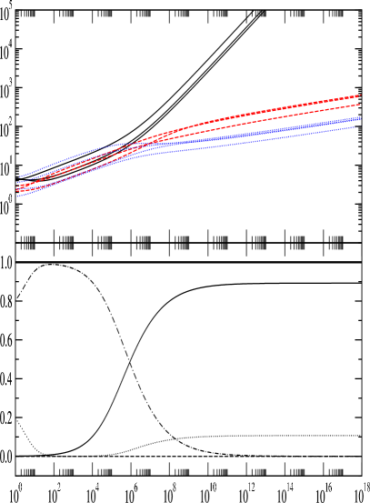
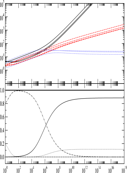
Figure 1: Cosmological evolution without fluxes. Graphs on the left are for a brane gas with a wrapping matrix of the type 3-3-4 and those on the right of the type 3-4-3. Plots on top represent the time evolution of the size (scale factor normalised by $2\pi$) of all the spatial dimensions: solid curves are for unwrapped dimensions, dashed curves for partially wrapped dimensions, and dotted curves for fully wrapped dimensions. Plots on the bottom depicts all the contributions to the expansion of the Universe as a function of cosmic time. The solid line represents $\Omega_{{}_{B}}$, the dashed line $\Omega_{{}_{G}}$, the dotted line $\Omega_{\sigma}$, and the dotted-dashed line $\Omega_{{}_{S}}$. The thick solid line is the sum of all the contributions and serves to check the accuracy of the numerical computation (29).

In conclusion, the cosmology of brane gases in a (low-energy) M theory context opens the possibility of explaining the number of spatial dimensions observed today for those configurations characterised by a wrapping parameter $m_{1}=3$. In the following we see that this conclusion is still true even if fluxes have a significant contribution at late times. Furthermore, we present new cosmological solutions with a larger number of initially unwrapped directions which support asymptotically a large four dimensional spacetime.

3.2 Cosmological evolution with fluxes

Now we are interested to investigate the influence of fluxes on the late-time cosmological dynamics of a Universe filled with a gas of M2-branes. The first difficulty one faces when fluxes are present is that the wrapping matrix describing the branes gas and the gauge field induce different splittings of the spacetime. As we have seen, the type of solutions for the 4-form field strength we are considering naturally separates the spacetime into R$\times$T³$\times$T⁷ and the gas of M2-branes into R$\times$T${}^{m_{1}}$$\times$T${}^{m_{2}}$$\times$T${}^{m_{3}}$. In spite of that, the universal power-law scaling behaviour at late times we have described in the previous section, although slightly modified, is not lost.

Given a brane gas configuration with wrapping matrix of type $m_{1}$-$m_{2}$-$m_{3}$ the late cosmological evolution can be cast into the form,

$$e^{\lambda_{i}}\sim\left\{\begin{array}[]{ll}t^{\alpha_{-}}&\textrm{\,\,\, for }i=1,\cdots,3\textrm{\,\, (unwrapped)}\\ t^{\alpha_{+}}&\textrm{\,\,\, for }i=4,\cdots,m_{1}\textrm{\,\, (unwrapped)}\\ t^{\beta}&\textrm{\,\,\, for }i=m_{1}+1,\cdots,m_{1}+m_{2}\textrm{\,\, (partially wrapped)}\\ t^{\gamma}&\textrm{\,\,\, for }i=m_{1}+m_{2}+1,\cdots,m_{1}+m_{2}+m_{3}\textrm{\,\, (fully wrapped)}\end{array}\right.$$ (34)

where we have chosen the first three directions to be those picked by the Freund-Rubin ansatz for the gauge field. As seen in Fig. 2, for configurations with a wrapping matrix 3-$m_{2}$-$m_{3}$, the energy density of the gauge field and the brane gas both have a significant contribution at late times. In this case (note that there are no directions with $\alpha_{+}$) the scaling behaviour is given analytically by,

$$\alpha_{-}=\frac{3}{7}\,,\,\,\,\,\,\,\,\beta=\gamma=\frac{1}{7}\,,$$ (35)

when $m_{2}<m_{3}$, and,

$$\alpha_{-}=\frac{5m_{2}m_{3}-14}{5m_{2}m_{3}+49}\,,\,\,\,\,\,\,\,\beta=\frac{5m_{3}(m_{2}-3)+7}{5m_{2}m_{3}+49}\,,\,\,\,\,\,\,\,\gamma=\frac{5m_{2}(m_{3}-3)+7}{5m_{2}m_{3}+49}\,,$$ (36)

when $m_{2}>m_{3}$. As a particular example of the last case, one has

$$\alpha_{-}=\frac{46}{109}\,,\,\,\,\,\,\,\,\beta=\frac{22}{109}\,,\,\,\,\,\,\,\,\gamma=\frac{7}{109}\,,$$ (37)

for $m_{2}=4$ and $m_{3}=3$. Comparing these results with (32) and (33) one readily observes that, although in both types of configurations the expansion rates of the unwrapped directions are decreased and those of the partially and fully wrapped are increased, the influence of fluxes at late times does not destroy the hierarchy between large and small dimensions ($\alpha_{-}$ is still greater than $\beta$ and $\gamma$ in all the cases). Note as well that even though the energy density of the gauge field fully dominates at early times, the energy density of the gas of branes very quickly takes over and the collapse of three dimensions is avoided. The appearance of a physical singularity in this early phase of the evolution is then prevented at the classical level.

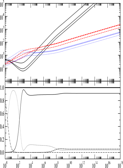
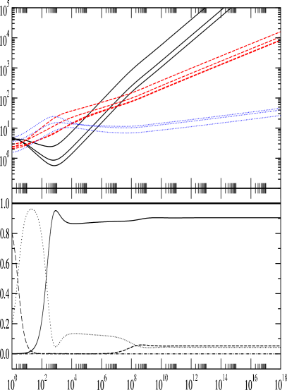
Figure 2: Cosmological dynamics of a brane gas of wrapping type 3-3-4 (left) and type 3-4-3 (right) with fluxes. The identification of plots and lines is the same as in Fig. 1.

A brane configuration of particular interest is that of a brane gas with 6 unwrapped dimensions; that is, configurations with wrapping matrix of type 6-$m_{2}$-$m_{3}$. Without fluxes, there are only four possible configurations leading to an anisotropic evolution. For all the configurations with $m_{2}\leq m_{3}$ one has the analytic solution (31) with,

$$\alpha=\frac{4}{11}\,,\,\,\,\,\,\,\,\beta=\gamma=-\frac{1}{11}\,.$$ (38)

On the other hand, for the configuration with wrapping 6-3-1, which is the only one with $m_{2}>m_{3}$ supporting a nonisotropic expansion, one obtains the scaling,

$$\alpha=\frac{23}{77}\,,\,\,\,\,\,\,\,\beta=\frac{8}{77}\,,\,\,\,\,\,\,\,\gamma=-\frac{22}{77}\,.$$ (39)

Obviously, if the dynamical effects of the gauge field are not taking into account these configurations, although providing a hierarchy among different dimensions, do not predict the right number of large spatial directions. Finally, it is important to note that, contrary to what happens when $m_{1}=3$, the energy density of the supergravity particles is always not negligible at late times.

Let us now consider the dynamical effects of the gauge degrees of freedom in configurations with $m_{1}=6$. Two numerical examples are compared with the no flux case in Figs. 3 and 4. An interesting point is that all the energy components ($\Omega_{{}_{B}},\Omega_{{}_{S}},\Omega_{{}_{G}}$) have a significant contribution to the cosmological expansion at late times. As one can also observe, these solutions represent a new family of configurations that permits the growth of three spatial dimensions. Although for the configuration with wrapping matrix 6-3-1 the hierarchy of the larger dimensions is not quite obvious from the plot obtained numerically (Fig. 4), it can be seen analytically that the asymptotic behaviour of the solution has the form (34) with,

$$\alpha_{-}=\frac{12}{44}\,,\,\,\,\,\,\,\,\beta=\frac{5}{44}\,,$$

$$\alpha_{+}=\frac{14}{44}\,,\,\,\,\,\,\,\,\gamma=-\frac{13}{44}\,.$$ (40)

The values obtained in our numerical computation agree with the above analytical result up to four decimal places. Comparing with the case without fluxes, $\beta$ is larger and $\gamma$ smaller. That means that the three partially wrapped dimensions grow faster and the fully wrapped dimension contracts also faster. On the other hand, the six unwrapped dimensions are separated into two groups, of three dimensions each, with independent expansion rates defined by $\alpha_{-}$ and $\alpha_{+}$, respectively. Since $\alpha_{-}<\alpha_{+}$ the appropriate hierarchy for explaining the number of spatial dimensions is produced. On the other hand, for $m_{2}\leq m_{3}$ one finds analogously the asymptotic power-laws (see Fig. 3),

$$\alpha_{-}=\frac{3}{11}\,,\,\,\,\,\,\,\,\alpha_{+}=\frac{5}{11}\,,\,\,\,\,\,\,\,\beta=\gamma=-\frac{1}{11}\,.$$ (41)

Again $\alpha_{+}>\alpha_{-}>\beta,\gamma$ and a hierarchy with three dimensions growing larger is obtained. Consequently, brane configurations with $m_{1}=6$ unwrapped dimensions can naturally explain why three large spatial dimensions are decompactified at late times if the gauge sector of eleven-dimensional supergravity is turned on. This new family of solutions enlarge the possible wrapping configurations at the end of brane-antibrane annihilation in the Hagedorn phase. It is important to emphasis that the interplay between both the brane gas and the flux dynamics plays a fundamental role in getting the correct number of large dimensions.

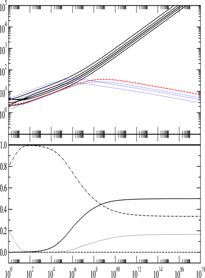
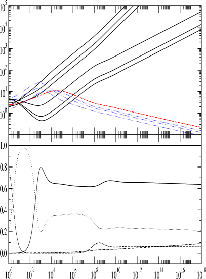
Figure 3: Cosmological dynamics of a brane gas of wrapping type 6-1-3 without (left) and with (right) fluxes. The identification of plots and lines is the same as in Fig. 1.

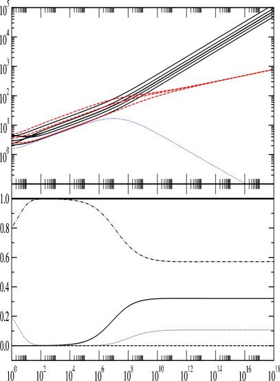
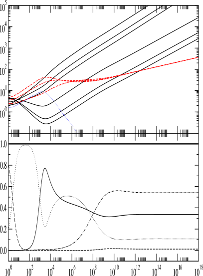
Figure 4: Cosmological dynamics of a brane gas of wrapping type 6-3-1 without (left) and with (right) fluxes. The identification of plots and lines is the same as in Fig. 1.

4 Conclusions

We have illustrated how the cosmological evolution at late time of a gas of M2-branes within a low-energy limit of M theory is modified when the gauge fields of the bosonic sector are taking into account.

We have seen that fluxes respect the hierarchies among different spatial dimensions introduced by an anisotropically wrapped brane gases at late times. We have also found new solutions that can explain the actual number of spatial dimensions of the Universe which are characterised by a brane gas configuration with a large number of unwrapped dimensions. These solutions appear as far as the gauge field strength is sufficiently strong to have a significant contribution to the total cosmological expansion at late times. On thermodynamical grounds one should expect that these brane configurations can be originated at the end of the Hagedorn phase from smaller initial spatial volumes of the Universe than configurations with lower unwrapping numbers. Including gauge fields into the dynamics increases the possible initial conditions for the Universe and then the probability of obtaining decompactification from anisotropically wrapped spacetimes. This makes less severe the fine-tuning problem posed by this mechanism when fluxes are not considered.

A difficult issue is to assess whether the constraints on the initial size of the Universe imposed by the holographic principle are significatively modified when gauge degrees of freedom are included. For the type of solutions we have studied the assumption of isotropy as considered in [27] is certainly not acceptable and a fully anisotropic analysis of entropy bounds is absolutely compulsory. In principle, the presence of a new physical parameter representing the strength of the gauge field opens the possibility of getting less restrictive conditions on the physical volume of the Universe in the Hagedorn phase.

Unfortunately, as in the case without fluxes, the internal dimensions do not stabilise for the physically interesting cases. In general, it seems rather difficult to get stabilisation within this mechanism without introducing additional physics.

Finally, it would be certainly interesting to investigate if there exist solutions with an even larger number of unwrapped dimensions that could as well explain the number of spacetime dimensions. A full classification of solutions and configurations will determine how generic is this anisotropic mechanism of decompactification. This analysis will further reveal the connection with the mechanism suggested in [15] within the context of ten-dimensional type IIA supergravity. This lower dimensional theory arises as a result of the compactification of eleven-dimensional supergravity and, thus, in principle, one should expect a close relationship between the cosmological solutions in both frameworks.

- [1] R. H. Brandenberger and C. Vafa, Superstrings in the early universe, Nucl. Phys. B316 (1989) 391.
- [2] A. A. Tseytlin and C. Vafa, Elements of string cosmology, Nucl. Phys. B372 (1992) 443–466, [hep-th/9109048].
- [3] A. A. Tseytlin, Dilaton, winding modes and cosmological solutions, Class. Quantum Grav. 9 (1992) 979–1000, [hep-th/9112004].
- [4] J. Kripfganz and H. Perlt, Cosmological impact of winding strings, Class. Quant. Grav. 5 (1988) 453.
- [5] B. A. Bassett, M. Borunda, M. Serone, and S. Tsujikawa, Aspects of string-gas cosmology at finite temperature, Phys. Rev. D67 (2003) 123506, [hep-th/0301180].
- [6] S. Alexander, R. H. Brandenberger, and D. Easson, Brane gases in the early universe, Phys. Rev. D62 (2000) 103509, [hep-th/0005212].
- [7] R. Brandenberger, D. A. Easson, and D. Kimberly, Loitering phase in brane gas cosmology, Nucl. Phys. B623 (2002) 421–436, [hep-th/0109165].
- [8] A. Campos, Late-time dynamics of brane gas cosmology, Phys. Rev. D68 (2003) 104017, [hep-th/0304216].
- [9] S. Watson and R. H. Brandenberger, Isotropization in brane gas cosmology, Phys. Rev. D67 (2003) 043510, [hep-th/0207168].
- [10] T. Boehm and R. Brandenberger, On t-duality in brane gas cosmology, JCAP 06 (2003) 008, [hep-th/0208188].
- [11] S. H. S. Alexander, Brane gas cosmology, m-theory and little string theory, JHEP 10 (2003) 013, [hep-th/0212151].
- [12] A. Kaya and T. Rador, Wrapped branes and compact extra dimensions in cosmology, Phys. Lett. B565 (2003) 19–26, [hep-th/0301031].
- [13] A. Kaya, On winding branes and cosmological evolution of extra dimensions in string theory, Class. Quant. Grav. 20 (2003) 4533–4550, [hep-th/0302118].
- [14] R. Brandenberger, D. A. Easson, and A. Mazumdar, Inflation and brane gases, Phys. Rev. D69 (2004) 083502, [hep-th/0307043].
- [15] A. Campos, Late cosmology of brane gases with a two-form field, Phys. Lett. B586 (2004) 133–139, [hep-th/0311144].
- [16] T. Biswas, Cosmology with branes wrapping curved internal manifolds, JHEP 02 (2004) 039, [hep-th/0311076].
- [17] S. Watson and R. Brandenberger, Linear perturbations in brane gas cosmology, JHEP 03 (2004) 045, [hep-th/0312097].
- [18] S. Watson, Uv perturbations in brane gas cosmology, Phys. Rev. D70 (2004) 023516, [hep-th/0402015].
- [19] S. Watson and R. Brandenberger, Stabilization of extra dimensions at tree level, JCAP 0311 (2003) 008, [hep-th/0307044].
- [20] T. Battefeld and S. Watson, Effective field theory approach to string gas cosmology, JCAP 0406 (2004) 001, [hep-th/0403075].
- [21] J. Y. Kim, Late time evolution of brane gas cosmology and compact internal dimensions, hep-th/0403096.
- [22] S. Watson, Moduli stabilization with the string higgs effect, hep-th/0404177.
- [23] A. Kaya, Volume stabilization and acceleration in brane gas cosmology, hep-th/0405099.
- [24] S. P. Patil and R. Brandenberger, Radion stabilization by stringy effects in general relativity and dilaton gravity, hep-th/0401037.
- [25] A. J. Berndsen and J. M. Cline, Dilaton stabilization in brane gas cosmology, hep-th/0408185.
- [26] R. Easther, B. R. Greene, M. G. Jackson, and D. Kabat, Brane gas cosmology in m-theory: Late time behavior, Phys. Rev. D67 (2003) 123501, [hep-th/0211124].
- [27] R. Easther, B. R. Greene, M. G. Jackson, and D. Kabat, Brane gases in the early universe: Thermodynamics and cosmology, JCAP 0401 (2004) 006, [hep-th/0307233].
- [28] R. Bousso, A covariant entropy conjecture, JHEP 07 (1999) 004, [hep-th/9905177].
- [29] R. Bousso, Holography in general space-times, JHEP 06 (1999) 028, [hep-th/9906022].
- [30] J. Demaret, J. L. Hanquin, M. Henneaux, and P. Spindel, Cosmological models in eleven-dimensional supergravity, Nucl. Phys. B252 (1985) 538–560.
- [31] E. Cremmer, B. Julia, and J. Scherk, Supergravity theory in 11 dimensions, Phys. Lett. B76 (1978) 409–412.
- [32] P. G. O. Freund and M. A. Rubin, Dynamics of dimensional reduction, Phys. Lett. B97 (1980) 233–235.
- [33] P. G. O. Freund, Kaluza-klein cosmologies, Nucl. Phys. B209 (1982) 146.
- [34] E. Alvarez, Cosmological solutions of n=1 supergravity in eleven- dimensions, Phys. Rev. D30 (1984) 1394. Erratum-ibid. D30, 2695 (1984).
- [35] R. G. Moorhouse and J. Nixon, Inflationary cosmology and 4 index tensor fields, Nucl. Phys. B261 (1985) 172.
- [36] S. P. de Alwis, A note on brane tension and m-theory, Phys. Lett. B388 (1996) 291–295, [hep-th/9607011].
- [37] E. Bergshoeff, E. Sezgin, and P. K. Townsend, Supermembranes and eleven-dimensional supergravity, Phys. Lett. B189 (1987) 75–78.