Abstract

In the present paper, we shall study the $4$-dimensional $Z_{2}$ lattice gauge model with a random gauge coupling; the random-plaquette gauge model(RPGM). The random gauge coupling at each plaquette takes the value $J$ with the probability $1-p$ and $-J$ with $p$. This model exhibits a confinement-Higgs phase transition. We numerically obtain a phase boundary curve in the $(p-T)$-plane where $T$ is the “temperature” measured in unit of $J/k_{B}$. This model plays an important role in estimating the accuracy threshold of a quantum memory of a toric code. In this paper, we are mainly interested in its “self-duality” aspect, and the relationship with the random-bond Ising model(RBIM) in $2$-dimensions. The “self-duality” argument can be applied both for RPGM and RBIM, giving the same duality equations, hence predicting the same phase boundary. The phase boundary curve obtained by our numerical simulation almost coincides with this predicted phase boundary at the high-temperature region. The phase transition is of first order for relatively small values of $p<0.08$, but becomes of second order for larger $p$. The value of $p$ at the intersection of the phase boundary curve and the Nishimori line is regarded as the accuracy threshold of errors in a toric quantum memory. It is estimated as $p=0.110\pm 0.002$, which is very close to the value conjectured by Takeda and Nishimori through the “self-duality” argument.

1 Introduction

The duality transformations provide us with important informations for certain class of statistical- and field-theoretical models. The most famous one is the Kramers-Wannier self-duality relation for the $2$-dimensional(2D) Ising spin model[1], which predicts the exact value of the critical temperature.

Its gauge-model counterpart was studied by Wegner[2, 3], and he showed that the $4$-dimensional Ising($Z_{2}$) lattice gauge theory is also self-dual. Its self-duality condition for the critical coupling constant is equivalent to that of the 2D Ising spin model, so the value of the critical coupling(temperature) coincides with that of the Ising model, though the orders of the phase transitions may be (and actually are) different in these two systems[4].

Recently, a duality transformation is applied for a random spin system of spin glass, the random-bond Ising model(RBIM) in two dimensions[5, 6]. This model contains a new parameter $p$, which controls the random quenched variables, i.e., the rate of nearest-neighbor spin-coupling with “wrong sign”. Thus the critical temperature becomes a function $T(p)$ of $p$. The “self-duality condition” for this model is proposed in order to locate the multicritical point[6]. The multicritical point is the intersection of the critical temperature $T(p)$ and the Nishimori line of spin glass. (More detailed discussion on this point will be given in Sec.2.) The duality transformation for the 2D RBIM is exact, but contrary to the nonrandom case ($p=0$), the proposed “self-duality condition” does not assure us that the singular point of the free energy is located at the “self-dual point”. However, once this “self-duality condition” is accepted, it allows us to make a conjecture on the location of $T(p)$. After that, this conjecture for RBIM has been verified by numerical simulation[7] for high-temperature region.

The 4-dimensional (4D) $Z_{2}$ random-plaquette gauge model(RPGM) plays an important role in the theory of quantum memory. Here the randomness $p$ is the probability that the gauge coupling for each plaquette takes the “wrong-sign”. (See Sect.2 for more details.) This model is used to predict the accuracy threshold of a 3-dimensional(3D) toric quantum code[8, 9, 10]. Actually, the accuracy threshold $p_{c}$ of the errors of a 3D toric quantum memory is determined by the multicritical point of the 4D RPGM[11]. The accuracy threshold of a 3D toric code $p_{c}$ is expected to be higher than that of a 2D toric code, $p_{c}=0.033$[12]. Thus it is quite important to obtain the phase boundary of the 4D RPGM.

Takeda and Nishimori[11, 13] applied the duality transformation for the 4D $Z_{2}$ RPGM, and assumed the “self-duality condition” in order to locate the multicritical point as $p_{c}=0.110028...$. The “self-duality condition” in the 4D $Z_{2}$ RPGM is the same with that of the 2D RBIM, and so the phase boundaries $T(p)$ of these two models are the same if the “self-duality condition” correctly predicts the phase boundary.

In this paper, we shall study the phase structure of the 4D RPGM by numerical simulation, in particular its confinement-Higgs phase transition. The result of the phase boundary curve shall be used to determine the accuracy threshold of a 3D toric code as well as to judge whether the “self-duality condition” proposed to determine $T(p)$ in Ref.[11, 13] is valid. We calculate the phase boundary curve, i.e., the critical temperature $T(p)$, in the $p-T$ plane. The curve $T(p)$ starts from the critical point of the nonrandom gauge model with the uniform coupling constant at $p=0$ and decreases as the randomness $p$ increases. Our result $T(p)$ is plotted in Fig.1 together with the result of “self-duality condition” of Ref.[11, 13] [See Eq.(9)]. The order of the phase transition is of first order for $p<0.08$, but it becomes of second order at larger values of $p$. We recall that the similar behavior in the order of phase transition is observed in the 3D RPGM, in which the phase transition changes from the second order transitions to the higher order ones[12]. Our curve $T(p)$ of the 4D RPGM coincides with the predicted phase boundary by the “self-duality conditions” of the both models mentioned above. This result verifies the conjecture by Takeda and Nishimori[11, 13] for the multicritical point of the 4D RPGM.

This paper is organized as follows. In Sec.2, we briefly review the duality transformation of the random models and show how the “self-duality condition” determines the critical curve in the $p-T$ plane. In Sec.3, we report our numerical calculations presenting the specific heat, the expectation values of the Wilson loops, and the fluctuations of the internal energy of the 4D RPGM, to determine the critical curve. Section 4 is devoted for conclusion.

2 Duality in the 4D random-plaquette gauge model

In this section we shall briefly review the duality transformation of the 4D RPGM following Ref.[11]. We consider the 4-dimensional hypercubic lattice, and put a $Z_{2}$ gauge variable $U_{x\mu}=\pm 1$ on each link $(x\mu)$, where $x$ denotes the site and $\mu=1,2,3,4$ is the index for four positive directions. The energy $H$ of the model is given by

$$H(U;\tau)=-J\sum_{P}\tau_{P}\prod_{P}U,$$ (1)

where $J(>0)$ is the strength of the (inverse) gauge coupling, $\prod_{P}U$ is the product of the four gauge variables $U_{x,\mu}$ on the four links surrounding the plaquette $P$. $\tau_{P}$ is the random variable for each plaquette $P$ taking $\tau_{P}=1$ with the probability $1-p$ and the “wrong-sign” $\tau_{P}=-1$ with the probability $p\ (\in[0,1])$.

We employ the replica technique for taking the ensemble averages over $\tau_{P}$. For the $n$-replica system, the averaged partition function $Z_{n}$ is given as

$$Z_{n}=\langle Z^{n}(\tau)\rangle_{\mbox{\footnotesize{ens}}},$$

$$Z^{n}(\tau)\equiv\Big{(}\prod_{\alpha=1}^{n}\sum_{U^{\alpha}_{x\mu}=\pm 1}\Big{)}\exp\Big{(}-\beta\sum_{\alpha=1}^{n}H(U^{\alpha};\tau)\Big{)},\ \beta\equiv\frac{1}{JT},$$ (2)

where $\alpha=1,\cdots,n$ is the replica index, and $\langle O(\tau)\rangle_{\mbox{\footnotesize{ens}}}$ denotes an ensemble average over $\{\tau_{P}\}$. The free energy $F$ is obtained by taking the limit $n\rightarrow 0$ as usual,

$$F = -\frac{1}{\beta}\lim_{n\rightarrow 0}\left(\frac{Z_{n}-1}{n}\right).$$ (3)

Let us introduce the Boltzmann weight for a single plaquette $P$, $\kappa_{+}=\exp(K)$ for the fluxless configurations $\prod_{P}U=1$ and the weight $\kappa_{-}=\exp(-K)$ for the fluxfull ones, where $K\equiv\beta J=1/T$. As we are considering $n$ replicas, it is useful to introduce the generalized Boltzmann weight for a single plaquette, i.e., for the configurations with fluxless $n-k$ replicas and fluxfull $k$ replicas, we assign the weight $x_{k}$ as[6, 11]

$$x_{k}=(1-p)\kappa_{+}^{n-k}\kappa_{-}^{k}+p\kappa_{+}^{k}\kappa_{-}^{n-k}.$$ (4)

Then the averaged partition function is expressed in terms of these weights, $x_{1},\cdots,x_{n}$,

$$Z_{n}=Z_{n}(x_{0},x_{1},\cdots,x_{n}).$$ (5)

To make a duality transformation, we introduce the dual Boltzmann weights $x^{\ast}_{k}\ (k=0,\cdots,n)$ by the following discrete Fourier transformations;

$$x^{\ast}_{2m} = {1\over 2^{n/2}}(\kappa_{+}+\kappa-)^{n-2m}(\kappa_{+}-\kappa_{-})^{2m},$$

$$x^{\ast}_{2m+1} = {1\over 2^{n/2}}(1-2p)(\kappa_{+}+\kappa-)^{n-2m-1}(\kappa_{+}-\kappa_{-})^{2m+1}.$$ (6)

Then the following duality relation can be derived[11],

$$Z_{n}(x_{0},x_{1},\cdots,x_{n})=Z_{n}(x^{\ast}_{0},x^{\ast}_{1},\cdots,x^{\ast}_{n}),$$ (7)

up to an irrelevant overall constant.

In the standard (nonrandom) $Z_{2}$ gauge model with $p=0$, it is known that a confinement-Higgs phase transition takes place at $K=K_{C}$ where $e^{-2K_{C}}=\sqrt{2}-1$. This critical value is obtained by imposing the self-duality condition $x_{0}=x_{0}^{*}$, with which the other $n$ conditions $x_{k}=x_{k}^{*}\;(k=1,\cdots,n)$ also hold (automatically) at $p=0$. Then it is expected that the phase boundary of the confinement-Higgs phase transition evolves starting at $(p=0,T=1/K_{C})$ into the region $0<p$. It is very interesting to see if the “self-duality condition”,

$$x_{0}=x_{0}^{\ast}$$ (8)

predicts not only the location of the multicritical point but also that of the whole phase boundary. Here we note that one cannot impose $n$ self-duality conditions $x_{k}=x_{k}^{*}\ (k=1,\cdots,n)$ simultaneously for $0<p$; these equations are overcomplete and have no solutions in contrast with the case of $p=0$. The arguments of the original and transformed partition functions are not equal even at the “self-dual point”. Therefore it is not necessarily assured that the “self-duality condition” (8) determines the singular point of $Z_{n}$.

Explicitly in the limit $n\rightarrow 0$, Eq.(8) reduces to the following equation,

$$p=-{1\over 2K}\log\Big{(}{1+e^{-2K}\over\sqrt{2}}\Big{)},$$ (9)

which determines the phase boundary curve $T(p)$ in the $p-T$ plane. The multicritical point is defined as the intersection point of the two curves, the phase boundary $T(p)$ and the Nishimori line defined by

$$\exp(-2K)=\frac{p}{1-p}.$$ (10)

The value $p=p_{C}$ at the multicritical point is regarded as the accuracy threshold for the error rate of a quantum memory of the 3D toric code[11, 12]. By using Eq.(9), Takeda and Nishimori[11] determined $p_{C}$ as $p_{C}=0.110028...$, which is considerably larger than the accuracy threshold $p_{c}=0.033$ for a 2D toric code[12], as it is naturally expected.

Here we comment on the 2D RBIM. In Ref.[5, 6], the duality transformation has been applied for the 2D RBIM. By imposing the same “self-duality condition” as Eq.(8), one obtains just Eq.(9), so these two models are predicted to have the same phase boundaries $T(p)$. The numerical simulation[14, 7] of the RBIM gives the phase boundary that almost coincides with Eq.(9) in the region of the $p-T$ plane above the Nishimori line (the high-$T$ region). As explained above, the “self-duality condition” for the random systems is just a conjecture, so it is interesting to see if it is satisfied also in the random gauge systems. The results of the 4D RPGM will be reported in the following section.

3 Numerical study of the 4D $Z_{2}$ RPGM

In this section, we shall show our results of numerical simulation for the phase structure of the 4D $Z_{2}$ RPGM, particularly whether the phase boundary of the confinement-Higgs phase transition coincides with the predicted curve (9). As explained in the introduction, there exists a confinement-Higgs phase transition in the nonrandom gauge theory with $p=0$, and the critical coupling is given as $K_{C}=-{1\over 2}\ln(\sqrt{2}-1)$ by the self-duality nature of the model. We expect that the phase boundary curve evolves from the point $(p=0,T=1/K_{C})$ downward as $p$ increases in the $p-T$ plane since the inclusion of random couplings tends to put the system in a disordered phase.

In our simulation, we first generate $\tau_{P}$ over the lattice randomly to prepare a sample. Then we perform Monte Carlo simulation of this sample with Metropolis algorithm. After repeating this procedure, we get the results of a set of samples. Finally we average these results over the samples. We calculated the following quantities;

1. Internal energy and specific heat

2. Expectation values of the Wilson loop and their deviations from the perimeter/area law

3. Fluctuations of internal energy and specific heat among samples

The internal energy and the specific heat are useful to determine the phase boundary and the order of the phase transition in the high-$T$ region. As we explained before, the high-$T$ region is the region above the Nishimori line in the $p-T$ plane. The second quantity, the Wilson loop, is an order parameter of the gauge theory[15]; it obeys the area law in the confinement phase, while it obeys the perimeter law in the deconfinement phase. In the present case, we use it to locate the phase boundary close to the Nishimori line in the high-$T$ region. The third quantity is used to identify the multicritical point, the intersection of the phase boundary curve and the Nishimori line. As it can be proved exactly, the specific heat (and the internal energy) shows no singular behavior on the Nishimori line[16, 12]. Then it is rather difficult to identify the phase transition point near the Nishimori line. We use all the above three quantities to identify the transition points.

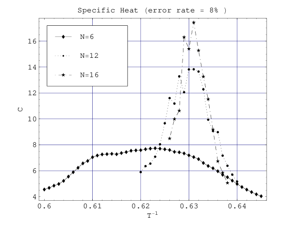
Figure 3: Lattice size dependence of the specific heat for $p=0.08$. The number of used samples is $\sim 10^{2}$.

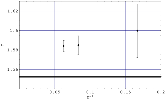
Figure 4: Lattice size dependence of the transition point for $p=0.08$. The bold line indicates the predicted value $T=1.552...$ by the “self-duality condition” (9).

In Fig.2, we plot the internal energy $\langle E\rangle$ and the specific heat $C$ per site at $p=0,0.02,0.04,0.06,0.08$ and $0.10$. It seems obvious that the phase transition is of first order for smaller value of $p$, $p<0.08$, whereas it becomes of second order for larger $p$. The critical points $T(p)$ in Fig.1 in the high-$T$ region are determined from these peaks of $C$. They are fairly in good agreements with the self-duality prediction (9), but there still exist small differences. We think that they are due to the finite-size effect. To check this point, we study the size-dependence of the specific heat. Fig.3 shows $C$ at $p=0.08$ for the lattice sizes $N^{4}$ with $N=6,12,16$. We observe that the peak of $C$ becomes sharper and higher for larger lattices, which verifies the second-order phase transition at $p=0.08$. The value of $T$ at the peak decreases gradually as $N$ increases. In Fig.4 the location of $T$ at the peak of $C$ is plotted versus the inverse of the linear size $N$ of the lattice. As $N$ increases, $T(p)$ gets closer to the predicted value $T(p=0.08)=1.552...$ by the self-duality condition (9).

Next let us see the expectation value of the Wilson loop (for the $Z_{2}$ gauge theory it was first introduced by Wegner [2]), $W(C)$, for a close loop $C$ on the lattice, which is defined as follows;

$$W(C) = \langle W(C,\tau)\rangle_{\mbox{\footnotesize{ens}}},$$

$$W(C,\tau) = \prod_{x\mu}\sum_{U_{x\mu}}\Big{(}\prod_{C}U_{x,\mu}\Big{)}\exp(-\beta H(U;\tau))/Z(\tau),$$

$$Z(\tau) = \prod_{x\mu}\sum_{U_{x\mu}}\exp(-\beta H(U;\tau)).$$ (11)

In the confinement phase of the gauge theory, $W(C)$ obeys what is called the area law,

$$W(C)\propto e^{-\alpha A(C)},$$ (12)

where $\alpha$ is a constant named string tension and $A(C)$ is the minimum value of the area of a membrane that covers the closed loop $C$. On the other hand, in the deconfinement phase, $W(C)$ obeys the perimeter law,

$$W(C)\propto e^{-\gamma P(C)},$$ (13)

where $\gamma$ is another constant and $P(C)$ is the perimeter of $C$.

We calculate $W(C)$ for various $p$’s with a fixed $K=1/T$ and fit the data by the area and perimeter laws. In Fig.5, the typical results near the multicritical point are shown. These results clearly show that $W(C)$ changes its behavior from the area law to the perimeter law as $p$ increases. In Fig.6, we present the results of $\chi^{2}$ fittings for $K=0.9$ and $1.0$. We can (roughly) estimate the phase transition point by using these results.

Finally, we study the fluctuations of $\langle E\rangle$ and $C$ over the samples. In the previous studies on the 2D RBIM and the 3D RPGM, it was observed that the fluctuations of these quantities indicate signals of the phase transition[17, 12]. In Fig.7, we present these fluctuations for $K=0.9$ and $1.0$. The fluctuation of $C$ stays almost constant at large $p$ (i.e., in the confinement phase), and it increases considerably as $p$ decreases and passes a certain critical value. The critical point of $p$ is very close to the phase transition point estimated by the other numerical calculations given above. More precisely, we estimate the values of $p$ at the criticality for $K=1.0$ as $p=0.110\pm 0.002$. Since this point is very close to the expected multicritical point as seen in Fig.1, we think that it is reasonable to use this value as the estimation of $p_{c}$ at the multicritical point.

4 Conclusion

In this paper we studied the 4D RPGM numerically. All the calculations consistently indicate the existence of the confinement-Higgs phase transition continuing from the nonrandom case $p=0$ to the random case $0<p$. The critical curve $T(p)$ is determined synthetically from $\langle E\rangle$, $C$, $W(C)$, and the fluctuations of $\langle E\rangle$ and $C$ over the samples. We summarize the results in Fig.1, which are in good agreement with the predicted value by the “self-duality condition” (9). In particular, our estimation of the multicritical point is $p_{c}=0.110\pm 0.002$, while the “self-duality condition” predicts $p=0.110228..$. We regard the small but non-negligible differences between the numerical result of $T(p)$ and (9) as the finite-size effect. Our studies strongly indicate the correctness of the conjecture by the “self-duality” (8) not only for the spin glass model but also for the random gauge model in the high-$T$ region. Numerical simulations of the random models at low-$T$ region require considerably many samples to obtain reliable ensemble averages[12], so we did not present $T(p)$ at the low-$T$ region below the Nishimori line in Fig.1. It is reserved for the future problem.

Acknowledgment

One of the authors (K.T.) would like to thank H. Nishimori, Y. Ozeki and T. Sasamoto for their suggestions and useful comments. He was supported by the Grant-in-Aid for Scientific Research on Priority Area “Statistical-Mechanical Approach to Probabilistic Information Processing” and the 21st Century COE Program at Tokyo Institute of Technology “Nanometer-Scale Quantum Physics”.

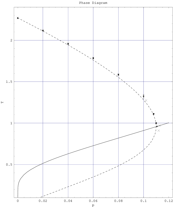
Figure 1: Phase diagram of the 4D RPGM and the 2D RBIM in the $p$(randomness)-$T$(temperature) plane. The diamond symbols show the transition points of the 4D RPGM obtained by our numerical study. The cross symbols show the transition points of the 2D RBIM calculated in Ref.[14]. The triangle symbol shows the transition point of the 2D RBIM on the Nishimori line calculated in Ref.[7]. The dashed curve is the phase boundary obtained by the “self-duality condition” (9), which predicts the same curve for the 4D RPGM and the 2D RBIM. This curve separate the confinement phase on the right-hand side (larger $p$) and the Higgs(deconfinement) phase on the left-hand side (smaller $p$). The solid curve is the Nishimori line (10), which is also identical for the two models.

Figure 2: Specific heat $C$ and internal energy $\langle E\rangle$ per site vs $1/T$ in the high-$T$ region for typical samples (from $p=0$ up to $p=0.1$). For $p<0.08$, $C$ exhibits a double-peak structure, and $\langle E\rangle$ exhibits hysteresis, both indicating that the phase transition is of first order. The lattice size is $16^{4}$ for $p=0.0$ and $12^{4}$ for the other $p$’s, and the typical sweep number is $3\times 10^{4}$ for $p=0$ and $5\times 10^{4}(p=2,4,6\%),10^{5}(p=8\%),2\times 10^{6}(p=10\%)$.

$T^{-1}=0.9$

$T^{-1}=1.0$

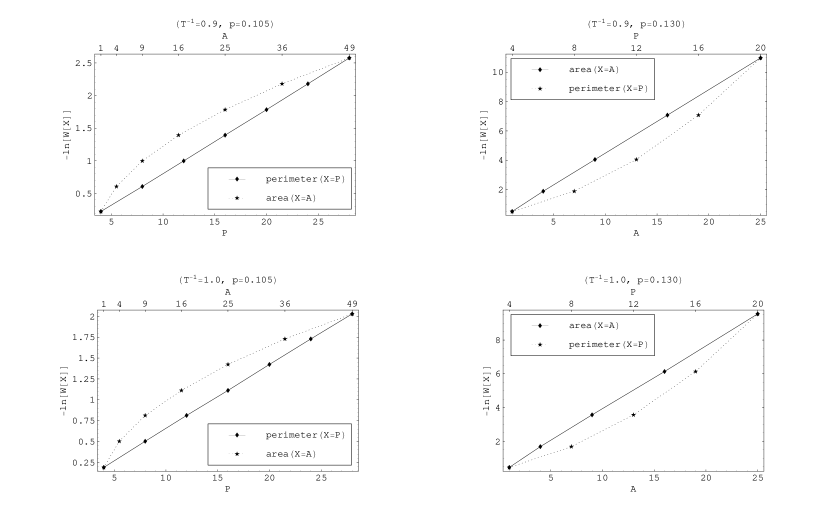
$p=0.105$                                             $p=0.13$

Figure 5: Wilson loops $W(C)$ for typical samples in the region near the Nishimori line. The lower(upper) horizontal axis $P$ denotes the perimeter of the loop $C$ for the perimeter-law fitting, and the upper(lower) horizontal axis $A$ denotes the area of C for the area-law fitting. The data show the perimeter(area)-law behavior for $p=0.105$($p=0.13$) in the left(right) column at each temperature. The lattice size is $10^{4}$, and the typical number of sweeps is $2\times 10^{4}$.

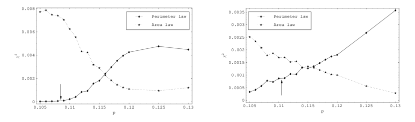
(a) $T^{-1}=0.9$                                             (b) $T^{-1}=1.0$

Figure 6: Deviation $\chi^{2}$ over 500 samples from the perimeter or area law vs $p$. $W(C)$ is normalized as $-\ln[W(C_{5})]=1$, where $C_{5}$ is the contour of a square whose area is $A(C_{5})=5^{2}$. The arrows show the transition points estimated from the specific heat and internal energy (see Fig.7).

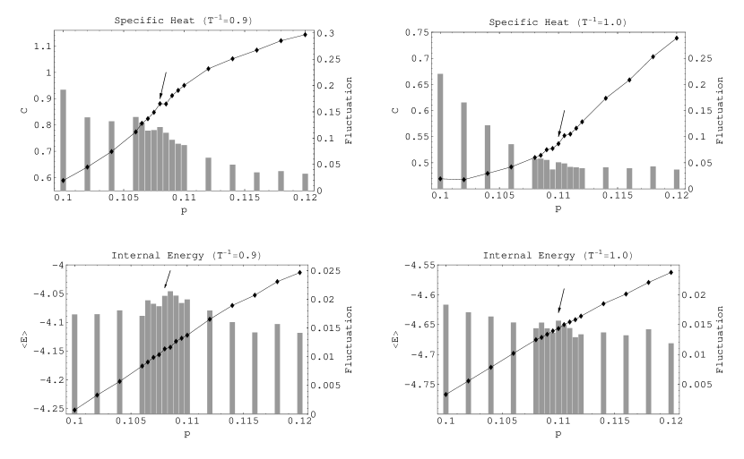
(a) $T^{-1}=0.9$                                             (b) $T^{-1}=1.0$

Figure 7: Specific heat and internal energy in the region near the Nishimori line. The histograms show their fluctuations among 200 samples. The arrows exhibit the phase transition points at which the magnitudes of fluctuations change their rate of variation with respect to $p$. The lattice size is $10^{4}$, and the typical number of sweeps is $2\times 10^{5}$.

References

- [1] H.A.Kramers and G.H.Wannier, Phys.Rev.60, 252(1941).
- [2] F.Wegner, J.Math.Phys.12, 2259(1971).
- [3] F.Y.Wu and Y.K.Wang, J.Math.Phys.17, 439(1976).
- [4] See, for example, M.Creutz, L.Jacobs and C.Rebbi, Phys.Reports 95, 201(1983).
- [5] H.Nishimori, J. Phys. C13, 4071(1980); Prog. Theor. Phys. 66, 1169(1981)
- [6] J.-M.Maillard, K.Nemoto, and H.Nishimori, J.Phys.A36, 9799(2003); H.Nishimori and K.Nemoto, J.Phys.Soc.Jpn.71, 1198(2002).
- [7] N.Ito and Y.Ozeki, Physica A312, 262(2003), and references cited therein.
- [8] A.Kitaev, Ann.Phys.303, 2(2003).
- [9] E.Dennis, A.Kitaev, A.Landahl, and J.Preskill, J.Math.Phys. 43, 4452(2002).
- [10] C.Wang, J.Harrington, and J.Preskill, Ann.Phys.303, 31(2003).
- [11] K.Takeda and H.Nishimori, Nucl.Phys.B686, 377(2004).
- [12] T.Ohno, G.Arakawa, I.Ichinose, and T.Matsui, quant-ph/0401101, “Phase structure of the random-plaquette gauge model: Accuracy threshold for a toric quantum memory”; Nucl.Phys.B (in press).
- [13] K.Takeda, T.Sasamoto and H.Nishimori, in preparation.
- [14] N.Ito, Y.Ozeki and H.Kitatani, J.Phys.Soc.Jpn.68, 803(1999).
- [15] K.Wilson, Phys.Rev.D10, 2445(1974).
- [16] H.Nishimori, “Statistical Physics of Spin Glasses and Information Processing”, (Oxford Univ.Press, Oxford, 2001).
- [17] H.Nishimori, C.Falvo and Y.Ozeki, J.Phys.A35, 8171(2002).
(a) (b)
(a) (b)