hep-th/0409045

KEK-TH-975

Membrane Fuzzy Sphere Dynamics
in Plane-Wave Matrix Model

Hyeonjoon Shin^a and Kentaroh Yoshida^b

^aBK 21 Physics Research Division and Institute of Basic Science
Sungkyunkwan University, Suwon 440-746, South Korea
^bTheory Division, High Energy Accelerator Research Organization (KEK)
Tsukuba, Ibaraki 305-0801, Japan

Abstract

In plane-wave matrix model, the membrane fuzzy sphere extended in the $SO(3)$ symmetric space is allowed to have periodic motion on a sub-plane in the $SO(6)$ symmetric space. We consider a background configuration composed of two such fuzzy spheres moving on the same sub-plane and the one-loop quantum corrections to it. The one-loop effective action describing the fuzzy sphere interaction is computed up to the sub-leading order in the limit that the mean distance $r$ between two fuzzy spheres is very large. We show that the leading order interaction is of the $1/r^{7}$ type and thus the membrane fuzzy spheres interpreted as giant gravitons really behave as gravitons.
Keywords : pp-wave, Matrix model, Fuzzy sphere
PACS numbers : 11.25.-w, 11.27.+d, 12.60.Jv

1 Introduction and Summary

The plane-wave matrix model [1] is a microscopic description of the discrete light cone quantized (DLCQ) M-theory in the eleven-dimensional $pp$-wave or plane-wave background [2], which is $SO(3)\times SO(6)$ symmetric and given by

$$ds^{2} =-2dx^{+}dx^{-}-\left(\sum^{3}_{i=1}\left(\frac{\mu}{3}\right)^{2}(x^{i})^{2}+\sum^{9}_{a=4}\left(\frac{\mu}{6}\right)^{2}(x^{a})^{2}\right)(dx^{+})^{2}+\sum^{9}_{I=1}(dx^{I})^{2}~{},$$

$$F_{+123} =\mu~{},$$ (1.1)

with the index notation $I=(i,a)$. It is now well known that this background is maximally supersymmetric and the limiting case of the eleven-dimensional $AdS$ type geometries [3]. Due to the effect of the $++$ component of the metric and the presence of the four-form field strength, the plane-wave matrix model has some $\mu$ dependent terms, which make the difference between the usual flat space matrix model [4] and the plane-wave one.

Compared to the flat matrix model, the plane-wave matrix model has some peculiar properties. One of them is that there are various supersymmetric vacuum structures classified by the $SU(2)$ algebra, which may be identified as collections of membrane fuzzy spheres [5]. Motivated by this classification, there have been further studies on the vacuum structure especially related to the protected multiplet [6], and various supersymmetric extended objects allowed by the plane-wave matrix model have been searched and studied [7, 8, 9, 10, 11, 12, 13, 14, 15, 16, 17]. There also have been studies on the thermodynamic properties of vacua [18].

The basic ingredient for vacua of plane-wave matrix model is the membrane fuzzy sphere which is interpreted as giant graviton. It preserves the full 16 supersymmetries of the plane-wave matrix model and exists even when the matrices have finite size $N$. Recently, based on the known properties of the membrane fuzzy sphere, we have tried to investigate the dynamical aspects of the plane-wave matrix model at the one-loop level and shown that two fuzzy spheres taking circular motion on a sub-plane of $SO(6)$ symmetric transverse space do not interact [19]. Single fuzzy sphere sitting at the origin of $SO(3)$ symmetric space and rotating in $SO(6)$ symmetric one is known to be a BPS object preserving 8 supersymmetries [12]. Our previous result implies that the configuration composed of two or more such fuzzy spheres rotating on the same sub-plane is also supersymmetric. This intriguing result however does not tell us about the dynamics of fuzzy spheres or giant gravitons.

In order to investigate the fuzzy sphere dynamics in plane-wave matrix model, it is then necessary to begin with a background configuration of fuzzy spheres which breaks supersymmetry explicitly. In this paper, we consider such a background and its one-loop quantum corrections. The resulting effective action describes the interaction between two fuzzy spheres, which respects the basic dynamical aspects of the plane-wave matrix model.

In the plane-wave matrix model, the static and supersymmetric fuzzy sphere is specified by the fine $N$-dimensional irreducible representation of $SU(2)$ and spans in the $SO(3)$ symmetric space. From now on, let us call $N$ the size of the fuzzy sphere. As will be discussed in Sec. 2, the equations of motion for the matrix variables allow it to have periodic motion. Let us consider a fuzzy sphere which has periodic motion on a sub-plane of the $SO(6)$ symmetric space (The $x^{4}$-$x^{5}$ plane is chosen in this paper). It has been known that it is supersymmetric when its periodic motion is circular, and otherwise it is not [12]. If we now consider a background configuration composed of two fuzzy spheres whose motions are circular and elliptic respectively in the $x^{4}$-$x^{5}$ plane, then it clearly breaks all the supersymmetry. The fuzzy sphere configuration taken in this paper is shown in Fig. 1 and will be described in more detail in Sec. 3. We note that the sizes of two fuzzy spheres are $N_{1}$ and $N_{2}$ respectively, and $N=N_{1}+N_{2}$.

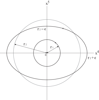
Figure 1: Configuration of two membrane fuzzy spheres moving in the $x^{4}$-$x^{5}$ plane. Since they span in the $SO(3)$ symmetric space, they are actually points in this plane. The first fuzzy sphere is in circular motion with the radius $r_{1}$. The second one takes an elliptic motion whose major and minor semi-axis are $r_{2}+\epsilon$ and $r_{2}-\epsilon$ respectively.

The plane-wave matrix model expanded around the fuzzy sphere is allowed to be studied perturbatively in the large $\mu$ limit [5]. In particular, in the limit of $\mu\rightarrow\infty$, only the quadratic action for the fluctuations around the fuzzy sphere background is important and hence the one-loop study gives exact results. In Sec. 3, this is justified again for our background, Fig. 1. The path integration of the quadratic action is performed in Sec. 4, where only the formal results are given. The actual calculation for obtaining the effective action is not easy due to the time dependent background given by trigonometric functions. At this stage, we need a proper parameter in terms of which the formal expressions of path integrations can be expanded perturbatively. It turns out that $\epsilon$ can be such a parameter if we assume that $\epsilon\ll|r_{2}-r_{1}|$, that is, the elliptic motion of the second fuzzy sphere is taken to be almost circular.

In Sec. 5, we present the perturbative calculation of the effective action in powers of $\epsilon$, and find that there are non-vanishing contributions from the $\epsilon^{4}$ order. The effective action describing the interaction between two fuzzy spheres is given by a function of $r$, $N_{1}$, and $N_{2}$, where $r\equiv r_{2}-r_{1}$ is the mean distance between two fuzzy spheres for one period of motion, and is evaluated in the long distance limit ($r\gg N$). Its explicit expression is obtained as

$$\Gamma_{\rm eff}=\epsilon^{4}\int dt\left[\frac{35}{2^{7}\cdot 3}\frac{N_{1}N_{2}}{r^{7}}-\frac{385}{2^{11}\cdot 3^{3}}\big{[}2(N_{1}^{2}+N_{2}^{2})-1\big{]}\frac{N_{1}N_{2}}{r^{9}}+\mathcal{O}\left(\frac{1}{r^{11}}\right)\right]+\mathcal{O}(\epsilon^{6})~{}.$$ (1.2)

In obtaining this effective action, there are contributions from the various sectors. The contributions themselves are presented in an appendix A. We note that, as will be discussed in Sec. 5, the effective action actually does not change even when $r_{1}>r_{2}$ and thus $r$ should be regarded as $|r|$. From the above effective action, we see that the leading order interaction is given by the form of $1/r^{7}$. This clearly shows that the two fuzzy spheres interpreted as giant gravitons really behave as gravitons.

2 Plane-wave matrix model and classical solutions

The plane-wave matrix model is basically composed of two parts. One part is the usual matrix model based on eleven-dimensional flat space-time, that is, the flat space matrix model, and another is a set of terms reflecting the structure of the maximally supersymmetric eleven dimensional plane-wave background, Eq. (1.1). Its action is

$$S_{pp}=S_{\mathrm{flat}}+S_{\mu}~{},$$ (2.1)

where each part of the action on the right hand side is given by

$$S_{\mathrm{flat}} =\int dt\mathrm{Tr}\left(\frac{1}{2R}D_{t}X^{I}D_{t}X^{I}+\frac{R}{4}([X^{I},X^{J}])^{2}+i\Theta^{\dagger}D_{t}\Theta-R\Theta^{\dagger}\gamma^{I}[\Theta,X^{I}]\right)~{},$$

$$S_{\mu} =\int dt\mathrm{Tr}\left(-\frac{1}{2R}\left(\frac{\mu}{3}\right)^{2}(X^{i})^{2}-\frac{1}{2R}\left(\frac{\mu}{6}\right)^{2}(X^{a})^{2}-i\frac{\mu}{3}\epsilon^{ijk}X^{i}X^{j}X^{k}-i\frac{\mu}{4}\Theta^{\dagger}\gamma^{123}\Theta\right)~{}.$$ (2.2)

Here, $R$ is the radius of circle compactification along $x^{-}$ and $D_{t}$ is the covariant derivative with the gauge field $A$,

$$D_{t}=\partial_{t}-i[A,\>]~{}.$$ (2.3)

The matrices $\gamma^{I}$ are the $SO(9)$ gamma matrices and satisfy the Clifford algebra

$$\{\gamma^{I},\gamma^{J}\}=2\delta^{IJ}~{}.$$ (2.4)

For dealing with the problem in this paper, it is convenient to rescale the gauge field and parameters as

$$A\rightarrow RA~{},~{}~{}~{}t\rightarrow\frac{1}{R}t~{},~{}~{}~{}\mu\rightarrow R\mu~{}.$$ (2.5)

With this rescaling, the radius parameter $R$ disappears and the actions in Eq. (2.2) become

$$S_{\mathrm{flat}} =\int dt\mathrm{Tr}\left(\frac{1}{2}D_{t}X^{I}D_{t}X^{I}+\frac{1}{4}([X^{I},X^{J}])^{2}+i\Theta^{\dagger}D_{t}\Theta-\Theta^{\dagger}\gamma^{I}[\Theta,X^{I}]\right)~{},$$

$$S_{\mu} =\int dt\mathrm{Tr}\left(-\frac{1}{2}\left(\frac{\mu}{3}\right)^{2}(X^{i})^{2}-\frac{1}{2}\left(\frac{\mu}{6}\right)^{2}(X^{a})^{2}-i\frac{\mu}{3}\epsilon^{ijk}X^{i}X^{j}X^{k}-i\frac{\mu}{4}\Theta^{\dagger}\gamma^{123}\Theta\right)~{}.$$ (2.6)

The possible backgrounds allowed by the plane-wave matrix model are the classical solutions of the equations of motion for the matrix fields. Since the background that we are concerned about is purely bosonic, we concentrate on solutions of the bosonic fields $X^{I}$. We would like to note that we will not consider all possible solutions but only those relevant to our interest for the fuzzy sphere interaction. Then, from the rescaled action, (2.6), the bosonic equations of motion are derived as

$$\ddot{X}^{i} =-[[X^{i},X^{I}],X^{I}]-\left(\frac{\mu}{3}\right)^{2}X^{i}-i\mu\epsilon^{ijk}X^{j}X^{k}~{},$$

$$\ddot{X}^{a} =-[[X^{a},X^{I}],X^{I}]-\left(\frac{\mu}{6}\right)^{2}X^{a}~{},$$ (2.7)

where the over dot implies the time derivative $\partial_{t}$.

Except for the trivial $X^{I}=0$ solution, the simplest one is the harmonic oscillator solution;

$$X^{i}_{\mathrm{osc}}=A^{i}\cos\left(\frac{\mu}{3}t+\phi_{i}\right){\bf 1}_{N\times N}~{},~{}~{}~{}X^{a}_{\mathrm{osc}}=A^{a}\cos\left(\frac{\mu}{6}t+\phi_{a}\right){\bf 1}_{N\times N}~{},$$ (2.8)

where $A^{I}$ and $\phi_{I}$ $(I=(i,a))$ are the amplitudes and phases of oscillations respectively, and ${\bf 1}_{N\times N}$ is the $N\times N$ unit matrix. This oscillatory solution is special to the plane-wave matrix model due to the presence of mass terms for $X^{I}$. It should be noted that, because of the mass terms, the configuration corresponding to the time dependent straight line motion, say $v^{I}t+c^{I}$ with non-zero constants $v^{I}$ and $c^{I}$, is not possible as a solution of (2.7), that is, a classical background of plane-wave matrix model, contrary to the case of the flat space matrix model. As the generalization of the oscillatory solution, Eq. (2.8), we get the solution of the form of diagonal matrix with each diagonal element having independent amplitude and phase.

As for the non-trivial constant matrix solution, Eq. (2.7) allows the following membrane fuzzy sphere or giant graviton solution:

$$X^{i}_{\mathrm{sphere}}=\frac{\mu}{3}J^{i}~{},$$ (2.9)

where $J^{i}$ satisfies the $SU(2)$ algebra,

$$[J^{i},J^{j}]=i\epsilon^{ijk}J^{k}~{}.$$ (2.10)

The reason why this solution is possible is basically that the matrix field $X^{i}$ feels an extra force due to the Myers interaction which may stabilize the oscillatory force. The fuzzy sphere solution $X^{i}_{\mathrm{sphere}}$ preserves the full 16 dynamical supersymmetries of the plane-wave and hence is 1/2-BPS object. We note that actually there is another fuzzy sphere solution of the form $\frac{\mu}{6}J^{i}$. However, it has been shown that such solution receives quantum corrections and hence is non-BPS object [10].

3 Expansion around fuzzy sphere configuration

In this section, the plane-wave matrix model is expanded around the fuzzy sphere configuration in which we are interested.

We first consider the expansion around the general background. For this, let us split the matrix quantities into as follows:

$$X^{I}=B^{I}+Y^{I}~{},~{}~{}~{}\Theta=F+\Psi~{},$$ (3.1)

where $B^{I}$ and $F$ are the general classical background fields satisfying the classical equations of motion, Eq. (2.7), while $Y^{I}$ and $\Psi$ are the quantum fluctuations around them. The fermionic background $F$ is taken to vanish from now on, since we will only consider the purely bosonic background. The quantum fluctuations are the fields subject to the path integration. In taking into account the quantum fluctuations, we should recall that the matrix model itself is a gauge theory. This implies that the gauge fixing condition should be specified before proceed further. In this paper, we take the background field gauge which is usually chosen in the matrix model calculation as

$$D_{\mu}^{\rm bg}A^{\mu}_{\rm qu}\equiv D_{t}A+i[B^{I},X^{I}]=0~{}.$$ (3.2)

Then the corresponding gauge-fixing $S_{\mathrm{GF}}$ and Faddeev-Popov ghost $S_{\mathrm{FP}}$ terms are given by

$$S_{\mathrm{GF}}+S_{\mathrm{FP}}=\int\!dt\,{\rm Tr}\left(-\frac{1}{2}(D_{\mu}^{\rm bg}A^{\mu}_{\rm qu})^{2}-\bar{C}\partial_{t}D_{t}C+[B^{I},\bar{C}][X^{I},\,C]\right)~{}.$$ (3.3)

Now by inserting the decomposition of the matrix fields (3.1) into Eqs. (2.6) and (3.3), we get the gauge fixed plane-wave action $S$ $(\equiv S_{pp}+S_{\mathrm{GF}}+S_{\mathrm{FP}})$ expanded around the background. The resulting action is read as

$$S=S_{0}+S_{2}+S_{3}+S_{4}~{},$$ (3.4)

where $S_{n}$ represents the action of order $n$ with respect to the quantum fluctuations and, for each $n$, its expression is

$$S_{0}=\int dt\,\mathrm{Tr}\bigg{[}\, \frac{1}{2}(\dot{B}^{I})^{2}-\frac{1}{2}\left(\frac{\mu}{3}\right)^{2}(B^{i})^{2}-\frac{1}{2}\left(\frac{\mu}{6}\right)^{2}(B^{a})^{2}+\frac{1}{4}([B^{I},\,B^{J}])^{2}-i\frac{\mu}{3}\epsilon^{ijk}B^{i}B^{j}B^{k}\bigg{]}~{},$$

$$S_{2}=\int dt\,\mathrm{Tr}\bigg{[}\, \frac{1}{2}(\dot{Y}^{I})^{2}-2i\dot{B}^{I}[A,\,Y^{I}]+\frac{1}{2}([B^{I},\,Y^{J}])^{2}+[B^{I},\,B^{J}][Y^{I},\,Y^{J}]-i\mu\epsilon^{ijk}B^{i}Y^{j}Y^{k}$$

$$-\frac{1}{2}\left(\frac{\mu}{3}\right)^{2}(Y^{i})^{2}-\frac{1}{2}\left(\frac{\mu}{6}\right)^{2}(Y^{a})^{2}+i\Psi^{\dagger}\dot{\Psi}-\Psi^{\dagger}\gamma^{I}[\Psi,\,B^{I}]-i\frac{\mu}{4}\Psi^{\dagger}\gamma^{123}\Psi$$

$$-\frac{1}{2}\dot{A}^{2}-\frac{1}{2}([B^{I},\,A])^{2}+\dot{\bar{C}}\dot{C}+[B^{I},\,\bar{C}][B^{I},\,C]\,\bigg{]}~{},$$

$$S_{3}=\int dt\,\mathrm{Tr}\bigg{[} -i\dot{Y}^{I}[A,\,Y^{I}]-[A,\,B^{I}][A,\,Y^{I}]+[B^{I},\,Y^{J}][Y^{I},\,Y^{J}]+\Psi^{\dagger}[A,\,\Psi]$$

$$-\Psi^{\dagger}\gamma^{I}[\Psi,\,Y^{I}]-i\frac{\mu}{3}\epsilon^{ijk}Y^{i}Y^{j}Y^{k}-i\dot{\bar{C}}[A,\,C]+[B^{I},\,\bar{C}][Y^{I},\,C]\,\bigg{]}~{},$$

$$S_{4}=\int dt\,\mathrm{Tr}\bigg{[} -\frac{1}{2}([A,\,Y^{I}])^{2}+\frac{1}{4}([Y^{I},\,Y^{J}])^{2}\bigg{]}~{}.$$ (3.5)

We now set up the background configuration for the membrane fuzzy spheres. Since we will study the interaction of two fuzzy spheres, the matrices representing the background have the $2\times 2$ block diagonal form as

$$B^{I}=\begin{pmatrix}B_{(1)}^{I}&0\\ 0&B_{(2)}^{I}\end{pmatrix}~{},$$ (3.6)

where $B_{(s)}^{I}$ with $s=1,2$ are $N_{s}\times N_{s}$ matrices. If we take $B^{I}$ as $N\times N$ matrices, then $N=N_{1}+N_{2}$.

The two fuzzy spheres are taken to be static in the space where they span, and hence represented by the classical solution, (2.9);

$$B_{(s)}^{i}=\frac{\mu}{3}J_{(s)}^{i}~{},$$ (3.7)

where, for each $s$, $J_{(s)}^{i}$ is in the $N_{s}$-dimensional irreducible representation of $SU(2)$ and satisfies the $SU(2)$ algebra, Eq. (2.10). In the $SO(6)$ symmetric transverse space, the fuzzy spheres are regarded as point objects, of course, in a sense of ignoring the matrix nature. We first take a certain two-dimensional sub-plane in the $SO(6)$ symmetric space. The two fuzzy spheres are then led to have periodic motion in this plane. More precisely, the first fuzzy sphere given by the background of $s=1$ is taken to be in circular motion with the radius $r_{1}$. As for the second fuzzy sphere, we take an elliptic motion whose major and minor semi-axis are $r_{2}+\epsilon$ and $r_{2}-\epsilon$ respectively. Obviously, this configuration is one of the classical solutions of the equations of motion as one can see from Eq. (2.8). Recalling that the transverse space is $SO(6)$ symmetric, all the possible choices of two-dimensional sub-plane where the periodic motion takes place are equivalent. Thus, without loss of generality, we can take an arbitrary plane for the periodic motion. In this paper, the $x^{4}$-$x^{5}$ plane is chosen. Then the configuration in the transverse space is given by

$$B^{4}_{(1)}=r_{1}\cos\left(\frac{\mu}{6}t\right){\bf 1}_{N_{1}\times N_{1}}~{},~{}~{}~{}B^{5}_{(1)}=r_{1}\sin\left(\frac{\mu}{6}t\right){\bf 1}_{N_{1}\times N_{1}}~{},$$

$$B^{4}_{(2)}=(r_{2}+\epsilon)\cos\left(\frac{\mu}{6}t\right){\bf 1}_{N_{2}\times N_{2}}~{},~{}~{}~{}B^{5}_{(2)}=(r_{2}-\epsilon)\sin\left(\frac{\mu}{6}t\right){\bf 1}_{N_{2}\times N_{2}}~{},$$ (3.8)

where $r_{1}$, $r_{2}$, and $\epsilon$ are non-negative. Eqs. (3.7) and (3.8) compose the background configuration about which we are concerned, and all other elements of matrices $B^{I}$ are set to zero. A schematic view of the background configuration is presented in Fig. 1. We would like to note that the fuzzy sphere represented by $B^{I}_{(1)}$ is supersymmetric [12]. However, since the fuzzy sphere in elliptic motion is not supersymmetric unless $\epsilon=0$, the whole configuration does not have supersymmetry. Although it is not necessary at the present stage, we assume that $\epsilon\ll r_{2}$ or $\epsilon\ll|r_{2}-r_{1}|$. As we shall see in later sections, the actual evaluation of the one-loop effective action requires a perturbative expansion parameter and the parameter $\epsilon$ can play a role of such parameter. Thus, the second fuzzy sphere is assumed to take an elliptic motion which is almost circular.

Actually, two fuzzy spheres may have their motions in different sub-planes in the $SO(6)$ symmetric space. The configuration taken here may be the simplest one. However, since our purpose is to investigate the very basic dynamical aspects of fuzzy spheres which are to be seen in every situations, it will be sufficient to consider only the simplest one among the possible configurations which seem to give non-trivial result. Indeed, as we shall see, the configuration given by Eqs. (3.7) and (3.8) leads to the basic but non-trivial interaction between two fuzzy spheres.

The classical value of the action for the background configuration,(3.7) and (3.8), is simply zero;

$$S_{0}=0~{}.$$ (3.9)

In the following sections, we are going to compute the one-loop correction to this action, that is, to the background, (3.7) and (3.8), due to the quantum fluctuations via the path integration of the quadratic action $S_{2}$, and obtain the one-loop effective action $\Gamma_{\mathrm{eff}}$ or the effective potential $V_{\mathrm{eff}}$.

For the justification of one-loop computation or the semi-classical analysis, it should be made clear that $S_{3}$ and $S_{4}$ of Eq. (3.5) can be regarded as perturbations. For this purpose, following [5], we rescale the fluctuations and parameters as

$$A\rightarrow\mu^{-1/2}A~{},~{}~{}~{}Y^{I}\rightarrow\mu^{-1/2}Y^{I}~{},~{}~{}~{}C\rightarrow\mu^{-1/2}C~{},~{}~{}~{}\bar{C}\rightarrow\mu^{-1/2}\bar{C}~{},$$

$$r_{1,2}\rightarrow\mu r_{1,2}~{},~{}~{}~{}\epsilon\rightarrow\mu\epsilon~{},~{}~{}~{}t\rightarrow\mu^{-1}t~{}.$$ (3.10)

Under this rescaling, the action $S$ in the background (3.7) and (3.8) becomes

$$S=S_{2}+\mu^{-3/2}S_{3}+\mu^{-3}S_{4}~{},$$ (3.11)

where $S_{2}$, $S_{3}$ and $S_{4}$ do not have $\mu$ dependence. Now it is obvious that, in the large $\mu$ limit, $S_{3}$ and $S_{4}$ can be treated as perturbations and the one-loop computation gives the sensible result.

Based on the structure of (3.6), we now write the quantum fluctuations in the $2\times 2$ block matrix form as follows:

$$A=\begin{pmatrix}0&\Phi^{0}\\ \Phi^{0\dagger}&0\end{pmatrix}~{},~{}~{}~{}Y^{I}=\begin{pmatrix}0&\Phi^{I}\\ \Phi^{I\dagger}&0\end{pmatrix}~{},~{}~{}~{}\Psi=\begin{pmatrix}0&\chi\\ \chi^{\dagger}&0\end{pmatrix}~{},$$

$$C=\begin{pmatrix}0&C\\ C^{\dagger}&0\end{pmatrix}~{},~{}~{}~{}\bar{C}=\begin{pmatrix}0&\bar{C}\\ \bar{C}^{\dagger}&0\end{pmatrix}~{}.$$ (3.12)

Although we denote the block off-diagonal matrices for the ghosts by the same symbols with those of the original ghost matrices, there will be no confusion since $N\times N$ matrices will never appear in what follows. The reason why the block-diagonal parts are taken to vanish is that they do not give any effect on the interaction between fuzzy spheres but lead to the quantum corrections to each fuzzy spheres. The issue about the path integral of block-diagonal fluctuations has been already considered in Refs. [10, 19], and it has been shown that each fuzzy sphere does not get quantum correction at least at one-loop order.

4 One-loop path integration

In this section, the path integration of $S_{2}$ is performed and the formal expression of the effective action $\Gamma_{\rm eff}$ is obtained. The resulting effective action will lead us to have informations about the interaction between two fuzzy spheres described by Eqs. (3.7) and (3.8).

The quadratic action $S_{2}$ may split into three pieces which do not couple with each other;

$$S_{2}=\int dt(L_{B}+L_{G}+L_{F})~{},$$ (4.1)

where $L_{G}$, $L_{G}$, and $L_{F}$ are the Lagrangians for the bosonic, ghost, and fermionic fluctuations of Eq. (3.12) respectively and their explicit expressions will be presented in due course. We note that there is no $\mu$ parameter in $S_{2}$ due to the rescaling (3.10), and hence the parameter does not appear in the one-loop effective action.

Let us begin with defining two useful quantities as

$$r\equiv r_{2}-r_{1}~{},~{}~{}~{}f(t)=\epsilon^{2}+2\epsilon r\cos(t/3)~{},$$ (4.2)

where $r$ is the mean distance between two fuzzy spheres. To express the formal results of path integrations compactly, some propagators are defined as follows.

$$G_{s}=\frac{1}{\partial_{t}^{2}+r^{2}+\frac{1}{3^{2}}(j+s)^{2}}~{},~{}~{}~{}(s=0,~{}1/2,~{}1)$$

$$G_{g}=\frac{1}{\partial_{t}^{2}+r^{2}+\frac{1}{3^{2}}j(j+1)}~{},$$ (4.3)

which appear in various places in this section.

In calculating the effective action, the prescription given by Kabat and Taylor [20] is usually used. It is well suited when the second and higher time derivatives of background can be ignored. At the present case, since the background is given by trigonometric functions, it may not be easy for their prescription to be adopted directly. As pointed out in [19], however, a simpler formulation is possible when we use the expansion in terms of the matrix spherical harmonics which has been done in[5]. The basic observation is that the $J^{i}$ representing the fuzzy sphere satisfies the $SU(2)$ algebra (2.10) and the fluctuation matrices in the theory can be regarded as $SU(2)$ representations. This leads to the appropriate form of the Lagrangian which makes the path integration be straightforward.

Let us note that the fluctuation matrices are $N_{1}\times N_{2}$ or $N_{2}\times N_{1}$ ones. This means that, if we regard an $N_{1}\times N_{2}$ block off-diagonal matrix as an $N_{1}N_{2}$-dimensional reducible representation of $SU(2)$, it has the decomposition into irreducible spin $j$ representations with the range $|N_{1}-N_{2}|/2\leq j\leq(N_{1}+N_{2})/2-1$, that is, $N_{1}N_{2}=\bigoplus_{j=|N_{1}-N_{2}|/2}^{(N_{1}+N_{2})/2-1}(2j+1)$. If we denote a generic fluctuation matrix as $\Phi$, then we have an expansion like

$$\Phi=\sum_{j=|N_{1}-N_{2}|/2}^{(N_{1}+N_{2})/2-1}\sum_{m=-j}^{j}\phi_{jm}Y^{N_{1}\times N_{2}}_{jm}~{},$$ (4.4)

where $Y^{N_{1}\times N_{2}}_{jm}$ is the $N_{1}\times N_{2}$ matrix spherical harmonics transforming in the irreducible spin $j$ representation and $\phi_{jm}$ is the corresponding spherical mode. This expansion allows us to write the Lagrangian in terms of the spherical modes and diagonalize some mass terms which are non-trivial products of fluctuation matrices. We will call the resulting Lagrangian as the diagonalized Lagrangian. One should notice that this does not mean that the diagonalized Lagrangian is the sum of free Lagrangians of spherical modes. Since the diagonalization is matrix diagonalization of mass terms, the Lagrangian may still have coupling terms between spherical modes even after the diagonalization. We note that, after the diagonalization, the spherical modes may have different ranges of $j$ if we keep $-j\leq m\leq j$. Since the whole procedure of diagonalization has been presented in Refs. [5, 19] and the diagonalizations in this paper proceed in exactly the same way, we will not go into any detail and only present the results. We also follow the same notations and conventions of [19] especially for the spherical modes.

4.1 Bosonic fluctuation

Let us first consider the bosonic Lagrangian and evaluate its path integral. The Lagrangian is

$$L_{B}=\mathrm{Tr}\bigg{[} -|\dot{\Phi}^{0}|^{2}+(r^{2}+f(t))|\Phi^{0}|^{2}+\frac{1}{3^{2}}\Phi^{0\dagger}J^{i}\circ(J^{i}\circ\Phi^{0})$$

$$+|\dot{\Phi}^{i}|^{2}-(r^{2}+f(t))|\Phi^{i}|^{2}-\frac{1}{3^{2}}|\Phi^{i}+i\epsilon^{ijk}J^{j}\circ\Phi^{k}|^{2}+\frac{1}{3^{2}}|J^{i}\circ\Phi^{i}|^{2}$$

$$+|\dot{\Phi}^{a}|^{2}-\Big{(}r^{2}+f(t)+\frac{1}{6^{2}}\Big{)}|\Phi^{a}|^{2}-\frac{1}{3^{2}}\Phi^{a\dagger}J^{i}\circ(J^{i}\circ\Phi^{a})$$

$$+\frac{i}{3}(r+\epsilon)\sin(t/6)(\Phi^{0\dagger}\Phi^{4}-\Phi^{4\dagger}\Phi^{0})-\frac{i}{3}(r-\epsilon)\cos(t/6)(\Phi^{0\dagger}\Phi^{5}-\Phi^{5\dagger}\Phi^{0})\,\bigg{]}~{}.$$ (4.5)

Here, adopting the notation of [5], we have defined

$$J^{i}\circ M_{(rs)}\equiv J^{i}_{(r)}M_{(rs)}-M_{(rs)}J^{i}_{(s)}~{},$$ (4.6)

where $M_{(rs)}$ is the $N_{r}\times N_{s}$ matrix that is a block at $r$-th row and $s$-th column in the blocked form of a given matrix $M$. In the present case, $r$ and $s$ take values of $1$ and $2$. For example, if we look at the $2\times 2$ block matrix form of the gauge field fluctuation $A$ in Eq. (3.12), then $A_{(ss)}=0$, $A_{(12)}=\Phi^{0}$, and $A_{(21)}=\Phi^{0\dagger}$.

The matrix fields, $\Phi^{0}$, $\Phi^{4}$, and $\Phi^{5}$ are coupled with each other through the fuzzy sphere background. In order to utilize the results of our previous work [19] where only the fuzzy spheres in circular motion have been considered, it is convenient to define the following matrix variables.

$$\Phi^{r}\equiv\cos(t/6)\Phi^{4}+\sin(t/6)\Phi^{5}~{},~{}~{}~{}\Phi^{\theta}\equiv-\sin(t/6)\Phi^{4}+\cos(t/6)\Phi^{5}~{}.$$ (4.7)

In terms of these fluctuations, the terms in the Lagrangian (4.5), which are dependent on $\Phi^{4}$ and $\Phi^{5}$, are rewritten as

$$\mathrm{Tr}\bigg{[} |\dot{\Phi}^{r}|^{2}+|\dot{\Phi}^{\theta}|^{2}-(r^{2}+f(t))\left(|\Phi^{r}|^{2}+|\Phi^{\theta}|^{2}\right)-\frac{1}{3^{2}}\left(\Phi^{r\dagger}J^{i}\circ(J^{i}\circ\Phi^{r})+\Phi^{\theta\dagger}J^{i}\circ(J^{i}\circ\Phi^{\theta})\right)$$

$$+\frac{1}{3}(\Phi^{r\dagger}\dot{\Phi}^{\theta}-\Phi^{\theta\dagger}\dot{\Phi}^{r})-\frac{i}{3}(r-\epsilon\cos(t/3))(\Phi^{0\dagger}\Phi^{\theta}-\Phi^{\theta\dagger}\Phi^{0})$$

$$+\frac{i}{3}\epsilon\sin(t/3)(\Phi^{0\dagger}\Phi^{r}-\Phi^{r\dagger}\Phi^{0})\bigg{]}~{}.$$ (4.8)

We observe that, because of the background for the motion in $x^{4}$-$x^{5}$ plane, the transverse $SO(6)$ symmetry is broken down to $SO(4)$, while the $SO(3)$ symmetry remains intact. This fact naturally leads us to break the bosonic Lagrangian (4.5) into three parts as follows:

$$L_{B}=L_{SO(3)}+L_{SO(4)}+L_{\rm rot}~{},$$ (4.9)

where $L_{SO(3)}$ is the Lagrangian for $\Phi^{i}$, $L_{SO(4)}$ is for $\Phi^{a^{\prime}}$ with $a^{\prime}=6,7,8,9$, and $L_{\rm rot}$ represents the rotational part described by $\Phi^{r}$, $\Phi^{\theta}$, and the gauge fluctuation $\Phi^{0}$.

We first consider $L_{SO(3)}$ and its path integration. The diagonalized Lagrangian describes the dynamics of two physical spherical modes, $\alpha_{jm}$ and $\beta_{jm}$, and one gauge mode, $\omega_{jm}$. Its explicit form is

$$L_{SO(3)}= \sum^{\frac{1}{2}(N_{1}+N_{2})-2}_{j=\frac{1}{2}|N_{1}-N_{2}|-1}\left[|\dot{\alpha}_{jm}|^{2}-\left(r^{2}+f(t)+\frac{1}{3^{2}}(j+1)^{2}\right)|\alpha_{jm}|^{2}\right]$$

$$+\sum^{\frac{1}{2}(N_{1}+N_{2})}_{j=\frac{1}{2}|N_{1}-N_{2}|+1}\left[|\dot{\beta}_{jm}|^{2}-\left(r^{2}+f(t)+\frac{1}{3^{2}}j^{2}\right)|\beta_{jm}|^{2}\right]$$

$$+\sum^{\frac{1}{2}(N_{1}+N_{2})-1}_{j=\frac{1}{2}|N_{1}-N_{2}|}\left[-|\dot{\omega}_{jm}|^{2}+\left(r^{2}+f(t)+\frac{1}{3^{2}}j(j+1)\right)|\omega_{jm}|^{2}\right]~{},$$ (4.10)

where the sum of $m$ over the range $-j\leq m\leq j$ is implicit. The path integral of this quadratic Lagrangian is straightforward and results in

$$e^{i\Gamma_{SO(3)}}= e^{i\Gamma_{SO(3)}^{(0)}}\left(\prod^{\frac{1}{2}(N_{1}+N_{2})-2}_{j=\frac{1}{2}|N_{1}-N_{2}|-1}\left[\det\left(1+G_{1}f(t)\right)\right]^{-(2j+1)}\right)$$

$$\times \left(\prod^{\frac{1}{2}(N_{1}+N_{2})}_{j=\frac{1}{2}|N_{1}-N_{2}|+1}\left[\det\left(1+G_{0}f(t)\right)\right]^{-(2j+1)}\right)$$

$$\times \left(\prod^{\frac{1}{2}(N_{1}+N_{2})-1}_{j=\frac{1}{2}|N_{1}-N_{2}|}\left[\det\left(G_{g}^{-1}+f(t)\right)\right]^{-(2j+1)}\right)~{},$$ (4.11)

where $\Gamma_{SO(3)}^{(0)}$ is the $\epsilon$ independent part from the path integration of the physical modes $\alpha_{jm}$ and $\beta_{jm}$, and its explicit form is

$$e^{i\Gamma_{SO(3)}^{(0)}}=\left(\prod^{\frac{1}{2}(N_{1}+N_{2})-2}_{j=\frac{1}{2}|N_{1}-N_{2}|-1}(\det G_{1}^{-1})^{-2j-1}\right)\left(\prod^{\frac{1}{2}(N_{1}+N_{2})}_{j=\frac{1}{2}|N_{1}-N_{2}|+1}(\det G_{0}^{-1})^{-2j-1}\right)~{}.$$

Since $\Gamma_{SO(3)}^{(0)}$ and other forthcoming $\epsilon$-independent parts have been already calculated in our previous work [19], we do not discuss about them in any detail but just quote the result that the sum of them vanishes basically due to supersymmetry, that is,

$$\sum_{n}\Gamma^{(0)}_{n}=0~{},$$ (4.12)

where $n$ indicates each physical sectors. The last determinant of Eq. (4.11) coming from the path integral of gauge modes $\omega_{jm}$ does not split into $\epsilon$ dependent and independent parts because it is eliminated by ghost contributions which will be given in the next subsection, that is, Eq. (4.21), and thus does not contribute to the total effective action $\Gamma_{\rm eff}$.

Let us turn to the bosonic $SO(4)$ part $L_{SO(4)}$. The corresponding spherical modes are $\phi^{a^{\prime}}_{jm}$ and the diagonalized Lagrangian is obtained as

$$L_{SO(4)}=\sum^{\frac{1}{2}(N_{1}+N_{2})-1}_{j=\frac{1}{2}|N_{1}-N_{2}|}\left[|\dot{\phi}^{a^{\prime}}_{jm}|^{2}-\left(r^{2}+f(t)+\frac{1}{3^{2}}\left(j+\frac{1}{2}\right)^{2}\right)|\phi^{a^{\prime}}_{jm}|^{2}\right]~{},$$ (4.13)

where $-j\leq m\leq j$ and $a^{\prime}=6,7,8,9$. Its path integration leads us to have

$$e^{i\Gamma_{SO(4)}}=e^{i\Gamma_{SO(4)}^{(0)}}\prod^{\frac{1}{2}(N_{1}+N_{2})-1}_{j=\frac{1}{2}|N_{1}-N_{2}|}\left[\det\left(1+G_{1/2}f(t)\right)\right]^{-4(2j+1)}~{},$$ (4.14)

where $e^{i\Gamma_{SO(4)}^{(0)}}=\prod^{\frac{1}{2}(N_{1}+N_{2})-1}_{j=\frac{1}{2}|N_{1}-N_{2}|}(\det G_{1/2}^{-1})^{-2j-1}$.

For the rotational part, the diagonalized Lagrangian describes the dynamics of three spherical modes, $\phi^{0}_{jm}$, $\phi^{r}_{jm}$, and $\phi^{\theta}_{jm}$, where the last two are the physical modes and $\phi^{0}_{jm}$ is the gauge one. The Lagrangian for these modes are

$$L_{\rm rot}=\sum^{\frac{1}{2}(N_{1}+N_{2})-1}_{j=\frac{1}{2}|N_{1}-N_{2}|}\Bigg{[} -|\dot{\phi}^{0}_{jm}|^{2}+\left(r^{2}+f(t)+\frac{1}{3^{2}}j(j+1)\right)|\phi^{0}_{jm}|^{2}$$

$$+|\dot{\phi}^{r}_{jm}|^{2}+|\dot{\phi}^{\theta}_{jm}|^{2}-\left(r^{2}+f(t)+\frac{1}{3^{2}}j(j+1)\right)\left(|\phi^{r}_{jm}|^{2}+|\phi^{\theta}_{jm}|^{2}\right)$$

$$+\frac{1}{3}(\phi^{r*}_{jm}\dot{\phi}^{\theta}_{jm}-\phi^{\theta*}_{jm}\dot{\phi}^{r}_{jm})-\frac{i}{3}(r-\epsilon\cos(t/3))(\phi^{0*}_{jm}\phi^{\theta}_{jm}-\phi^{\theta*}_{jm}\phi^{0}_{jm})$$

$$+\frac{i}{3}\epsilon\sin(t/3)(\phi^{0*}_{jm}\phi^{r}_{jm}-\phi^{r*}_{jm}\phi^{0}_{jm})\Bigg{]}~{},$$ (4.15)

where $-j\leq m\leq j$. Although the Lagrangian is quadratic in fields, the direct path integration is not so easy even at the formal level because of the explicit time dependent background. In order to do the path integration without any ambiguity, we first decouple the gauge mode from the other modes by performing a field redefinition,

$$\phi^{0}_{jm}\longrightarrow\phi^{0}_{jm}-\frac{i}{3}G_{g}\left[\epsilon\sin(t/3)\phi^{r}_{jm}-(r-\epsilon\cos(t/3))\phi^{\theta}_{jm}\right]~{}.$$

The modes $\phi^{r}_{jm}$ and $\phi^{\theta}_{jm}$ are still coupled with each other and the terms depending on them contain more complicated dependence of time dependent background after the above redefinition. For doing the path integration, we put the terms into the form of $v^{\dagger}Mv$ where $v$ is a two component column vector defined as $v=\begin{pmatrix}\phi^{r}_{jm}\\ \phi^{\theta}_{jm}\end{pmatrix}$, and $M$ is the $2\times 2$ matrix whose components are determined by the Lagrangian. Then the path integration of $\phi^{r}_{jm}$ and $\phi^{\theta}_{jm}$ is just that of $v$, which can be done by applying the following identity to the matrix $M$.

$$\begin{pmatrix}A&B\\ C&D\end{pmatrix}=\begin{pmatrix}A&0\\ C&1\end{pmatrix}\begin{pmatrix}1&A^{-1}B\\ 0&D-CA^{-1}B~{}.\end{pmatrix}$$ (4.16)

The resulting formal expressions of the path integrations is then obtained as

$$e^{i\Gamma_{\rm rot}}= e^{i\Gamma_{\rm rot}^{(0)}}\prod^{\frac{1}{2}(N_{1}+N_{2})-1}_{j=\frac{1}{2}|N_{1}-N_{2}|}\Bigg{[}\det\left(1+G_{g}f(t)+\frac{\epsilon^{2}}{3^{2}}G_{g}\sin(t/3)\frac{1}{G_{g}^{-1}+f(t)}\sin(t/3)\right)$$

$$\times \det\left(G_{0}G_{1}G_{g}^{-1}K\right)\det\left(G_{g}^{-1}+f(t)\right)\Bigg{]}^{-(2j+1)}~{},$$ (4.17)

where $e^{i\Gamma_{\rm rot}^{(0)}}=\prod^{\frac{1}{2}(N_{1}+N_{2})-1}_{j=\frac{1}{2}|N_{1}-N_{2}|}(\det G_{0}^{-1}G_{1}^{-1})^{-2j-1}$ and we have defined

$$K\equiv G_{g}^{-1}+f(t)+\frac{1}{3^{2}}(r-\epsilon\cos(t/3))\frac{1}{G_{g}^{-1}+f(t)}(r-\epsilon\cos(t/3))$$

$$+ \frac{1}{3^{2}}\left(\partial_{t}-\frac{\epsilon}{3}(r-\epsilon\cos(t/3))\frac{1}{G_{g}^{-1}+f(t)}\sin(t/3)\right)$$

$$\times\left(G_{g}^{-1}+f(t)+\frac{\epsilon^{2}}{3^{2}}\sin(t/3)\frac{1}{G_{g}^{-1}+f(t)}\sin(t/3)\right)^{-1}$$

$$\times\left(\partial_{t}+\frac{\epsilon}{3}\sin(t/3)\frac{1}{G_{g}^{-1}+f(t)}(r-\epsilon\cos(t/3))\right)~{}.$$ (4.18)

The last determinant factor in (4.17) comes from the path integral of the gauge mode. We note that $G_{0}G_{1}G_{g}^{-1}K=1+\mathcal{O}(\epsilon)$ and thus the second determinant factor in (4.17) does not involve non-trivial $\epsilon$ independent part.

4.2 Ghost fluctuation

We turn to the consideration of the path integration for the ghost part of the action $S_{2}$ (4.1). The Lagrangian for the ghosts is

$$L_{G}=\mathrm{Tr}\bigg{[}\, \dot{\bar{C}}\dot{C}^{\dagger}-(r^{2}+f(t))\bar{C}C^{\dagger}+\frac{1}{3^{2}}(J^{i}\circ\bar{C})(J^{i}\circ C^{\dagger})\,\bigg{]}$$

$$+\mathrm{Tr}\bigg{[}\, \dot{\bar{C}}^{\dagger}\dot{C}-(r^{2}+f(t))\bar{C}^{\dagger}C+\frac{1}{3^{2}}(J^{i}\circ\bar{C}^{\dagger})(J^{i}\circ C)\,\bigg{]}\,.$$ (4.19)

The spherical modes of $C$ and $\bar{C}$ in the matrix spherical harmonics expansion are $c_{jm}$ and $\bar{c}_{jm}$ respectively. The diagonalized Lagrangian is then obtained as

$$L_{G}=\sum^{\frac{1}{2}(N_{1}+N_{2})-1}_{j=\frac{1}{2}|N_{1}-N_{2}|}\Bigg{[}\,\dot{\bar{c}}^{*}_{jm}\dot{c}^{\dagger}_{jm}+\dot{\bar{c}}^{\dagger*}_{jm}\dot{c}_{jm}-\left(r^{2}+f(t)+\frac{1}{3^{2}}j(j+1)\right)(\bar{c}^{*}_{jm}c^{\dagger}_{jm}+\bar{c}^{\dagger*}_{jm}c_{jm})\,\Bigg{]}\,,$$ (4.20)

where the sum over $m$ for the range $-j\leq m\leq j$ is implicit. The path integral for the above diagonalized Lagrangian is then immediately evaluated as follows:

$$\prod^{\frac{1}{2}(N_{1}+N_{2})-1}_{j=\frac{1}{2}|N_{1}-N_{2}|}\left[\det\left(G_{g}^{-1}+f(t)\right)\right]^{2(2j+1)}~{}.$$ (4.21)

As we mentioned earlier, this eliminates the last determinant factors of (4.11) and (4.17) resulting from the path integrations of the gauge modes. Thus there is no contribution of the gauge and ghost modes to the total effective action, as it should be. Then the physical bosonic effective action $\Gamma_{B}$ is now given by

$$\Gamma_{B}=\widehat{\Gamma}_{SO(3)}+\Gamma_{SO(4)}+\widehat{\Gamma}_{\rm rot}~{},$$ (4.22)

where $\widehat{\Gamma}_{SO(3)}$ and $\widehat{\Gamma}_{\rm rot}$ are the same as those of Eqs. (4.11) and (4.17) except for the absence of the gauge mode contributions.

4.3 Fermionic fluctuation

The fermionic Lagrangian is

$$L_{F}=2\mathrm{Tr}\bigg{[}\, i\chi^{\dagger}\dot{\chi}-i\frac{1}{4}\chi^{\dagger}\gamma^{123}\chi+\frac{1}{3}\chi^{\dagger}\gamma^{i}J^{i}\circ\chi-r\chi^{\dagger}\left(\gamma^{4}\cos(t/6)+\gamma^{5}\sin(t/6)\right)\chi$$

$$-\epsilon\chi^{\dagger}\left(\gamma^{4}\cos(t/6)-\gamma^{5}\sin(t/6)\right)\chi\,\bigg{]}~{}.$$ (4.23)

It is convenient to introduce the $SU(2)\times SU(4)$ formulation since the preserved symmetry in the plane-wave matrix model is $SO(3)\times SO(6)\sim SU(2)\times SU(4)$ rather than $SO(9)$. In this formulation the $SO(9)$ spinor $\chi$ is decomposed as $\chi_{A\alpha}$ and $\hat{\chi}^{A\beta}$ according to ${\bf 16}\rightarrow({\bf 2},{\bf 4})+(\bar{\bf 2},\bar{\bf 4})$, where $A$ implies a fundamental $SU(4)$ index and $\alpha$ is a fundamental $SU(2)$ index. According to this decomposition, we may take the expression of $\chi$ as

$$\chi=\frac{1}{\sqrt{2}}\begin{pmatrix}\chi_{A\alpha}\\ \hat{\chi}^{A}_{\alpha}\end{pmatrix}~{},$$ (4.24)

where $\hat{\chi}^{A}_{\alpha}=\epsilon_{\alpha\beta}\hat{\chi}^{A\beta}$. We also rewrite the $SO(9)$ gamma matrices $\gamma^{I}$’s in terms of $SU(2)$ and $SU(4)$ ones as follows:

$$\gamma^{i}=\begin{pmatrix}-\sigma^{i}\times 1&0\\ 0&\sigma^{i}\times 1\end{pmatrix}\,,\quad\gamma^{a}=\begin{pmatrix}0&1\times\rho^{a}\\ 1\times(\rho^{a})^{\dagger}&0\end{pmatrix}\,,$$ (4.25)

where the $\sigma^{i}$’s are the standard $2\times 2$ Pauli matrices and six of $\rho^{a}$ are taken to form a basis of $4\times 4$ anti-symmetric matrices. The original $SO(9)$ Clifford algebra (2.4) is satisfied as long as we take normalization so that the gamma matrices $\rho^{a}$ with $SU(4)$ indices satisfy the algebra

$$\rho^{a}\rho^{b\dagger}+\rho^{b}\rho^{a\dagger}=2\delta^{ab}\,.$$ (4.26)

To work in parallel with our previous work [19], we now redefine the fermionic field $\hat{\chi}^{A}_{\alpha}$ as

$$\hat{\chi}^{A}_{\alpha}\equiv\left[(\rho^{4\dagger})^{AB}\cos(t/6)+(\rho^{5\dagger})^{AB}\sin(t/6)\right]\tilde{\chi}_{B\alpha}~{},$$ (4.27)

where we have introduced a new fermionic field $\tilde{\chi}_{A\alpha}$ which is in the ${\bf 4}$ of $SU(4)$. Then, by using the decomposed form of $\chi$ (4.24) with this redefinition and the following identities,

$$\left(\rho^{4}\cos(t/6)+\rho^{5}\sin(t/6)\right)\left(\rho^{4\dagger}\cos(t/6)+\rho^{5\dagger}\sin(t/6)\right)=1~{},$$

$$\left(\rho^{4}\cos(t/6)+\rho^{5}\sin(t/6)\right)\left(-\rho^{4\dagger}\sin(t/6)+\rho^{5\dagger}\cos(t/6)\right)=\rho^{4}\rho^{5\dagger}~{},$$ (4.28)

which are proved via the Clifford algebra (4.26), we may show that the Lagrangian (4.23) becomes

$$L_{F}=\mathrm{Tr}\bigg{[} i\chi^{\dagger A\alpha}\dot{\chi}_{A\alpha}-\frac{1}{4}\chi^{\dagger A\alpha}\chi_{A\alpha}-\frac{1}{3}\chi^{\dagger A\alpha}(\sigma^{i})_{\alpha}{}^{\beta}J^{i}\circ\chi_{A\beta}$$

$$+i\tilde{\chi}^{\dagger A\alpha}\dot{\tilde{\chi}}_{A\alpha}+\frac{1}{4}\tilde{\chi}^{\dagger A\alpha}\tilde{\chi}_{A\alpha}+\frac{1}{3}\tilde{\chi}^{\dagger A\alpha}(\sigma^{i})_{\alpha}{}^{\beta}J^{i}\circ\tilde{\chi}_{A\beta}$$

$$-\left(r+\epsilon\cos(t/3)\right)\left(\chi^{\dagger A\alpha}\tilde{\chi}_{A\alpha}+\tilde{\chi}^{\dagger A\alpha}\chi_{A\alpha}\right)+\frac{i}{6}\tilde{\chi}^{\dagger A\alpha}(\rho^{4}\rho^{5\dagger})_{A}{}^{B}\tilde{\chi}_{B\alpha}$$

$$-\epsilon\sin(t/3)\left(\chi^{\dagger A\alpha}(\rho^{4}\rho^{5\dagger})_{A}{}^{B}\tilde{\chi}_{B\alpha}-\tilde{\chi}^{\dagger A\alpha}(\rho^{4}\rho^{5\dagger})_{A}{}^{B}\chi_{B\alpha}\right)\bigg{]}\,.$$ (4.29)

For obtaining the diagonalized Lagrangian, we first take the expansion of $\chi_{\alpha}$ and $\tilde{\chi}_{\alpha}$ ($SU(4)$ indices are suppressed.) in terms of the matrix spherical harmonics like (4.4) and denote their spherical modes as $(\chi_{\alpha})_{jm}$ and $(\tilde{\chi}_{\alpha})_{jm}$ respectively. The diagonalization of the mass terms for the modes is that for the $SU(2)$ indices and results in $(\chi_{\alpha})_{jm}\rightarrow(\pi_{jm},\eta_{jm})$ and $(\tilde{\chi}_{\alpha})_{jm}\rightarrow(\tilde{\pi}_{jm},\tilde{\eta}_{jm})$. The modes $\pi_{jm}$ and $\tilde{\pi}_{jm}$ have the same $j$-dependent mass of $\frac{1}{3}(j+\frac{3}{4})$ with $\frac{1}{2}|N_{1}-N_{2}|-\frac{1}{2}\leq j\leq\frac{1}{2}(N_{1}+N_{2})-\frac{3}{2}$. For the modes $\eta_{jm}$ and $\tilde{\eta}_{jm}$, their $j$-dependent mass is $\frac{1}{3}(j+\frac{1}{4})$ with $\frac{1}{2}|N_{1}-N_{2}|+\frac{1}{2}\leq j\leq\frac{1}{2}(N_{1}+N_{2})-\frac{1}{2}$. All the modes have the same range of $m$ as $-j\leq m\leq j$. Having the spherical modes leading to the diagonalization for the $SU(2)$ indices, we turn to the consideration of terms containing $\rho^{4}\rho^{5\dagger}$. The product $\rho^{4}\rho^{5\dagger}$ measures the $SO(2)$ chirality in the $x^{4}$-$x^{5}$ plane where the fuzzy spheres take their motion. Since $(\rho^{4}\rho^{5\dagger})^{2}=-1$, its eigenvalues are $\pm i$. Each spherical mode may split into modes having definite $\rho^{4}\rho^{5\dagger}$ eigenvalues as follows:

$$\pi_{jm}=\pi_{+jm}+\pi_{-jm}~{}, \eta_{jm}=\eta_{+jm}+\eta_{-jm}~{},$$

$$\tilde{\pi}_{jm}=\tilde{\pi}_{+jm}+\tilde{\pi}_{-jm}~{}, \tilde{\eta}_{jm}=\tilde{\eta}_{+jm}+\tilde{\eta}_{-jm}~{},$$ (4.30)

where the modes on the right hand sides satisfy

$$\rho^{4}\rho^{5\dagger}\pi_{\pm jm}=\pm i\pi_{\pm jm}~{}, \rho^{4}\rho^{5\dagger}\tilde{\pi}_{\pm jm}=\pm i\tilde{\pi}_{\pm jm}~{},$$

$$\rho^{4}\rho^{5\dagger}\eta_{\pm jm}=\pm i\eta_{\pm jm}~{}, \rho^{4}\rho^{5\dagger}\tilde{\eta}_{\pm jm}=\pm i\tilde{\eta}_{\pm jm}~{}.$$ (4.31)

After splitting the modes according the $SO(2)$ chirality as in (4.30), we now have eight kinds of fermionic spherical modes in total, in terms of which the fermionic Lagrangian (4.29) is diagonalized. The resulting Lagrangian is composed of two independent systems as follows.

$$L_{F}=L_{\pi}+L_{\eta}~{}.$$ (4.32)

The first one $L_{\pi}$, which we call $\pi$-system, is for $\pi_{\pm jm}$ and $\tilde{\pi}_{\pm jm}$, and the other one $L_{\eta}$, that is $\eta$-system, for $\eta_{\pm jm}$ and $\tilde{\eta}_{\pm jm}$. The Lagrangian for the $\pi$-system is given by

$$L_{\pi}= \sum_{j=\frac{1}{2}|N_{1}-N_{2}|-\frac{1}{2}}^{\frac{1}{2}(N_{1}+N_{2})-\frac{3}{2}}\Bigg{[}\,i\pi_{+jm}^{\dagger}\dot{\pi}_{+jm}+i\pi_{-jm}^{\dagger}\dot{\pi}_{-jm}-\frac{1}{3}\left(j+\frac{3}{4}\right)(\pi^{\dagger}_{+jm}\pi_{+jm}+\pi^{\dagger}_{-jm}\pi_{-jm})$$

$$+i\tilde{\pi}_{+jm}^{\dagger}\dot{\tilde{\pi}}_{+jm}+\frac{1}{3}\left(j+\frac{1}{4}\right)\tilde{\pi}^{\dagger}_{+jm}\tilde{\pi}_{+jm}+i\tilde{\pi}_{-jm}^{\dagger}\dot{\tilde{\pi}}_{-jm}+\frac{1}{3}\left(j+\frac{5}{4}\right)\tilde{\pi}^{\dagger}_{-jm}\tilde{\pi}_{-jm}$$

$$-\left(r+\epsilon e^{it/3}\right)(\pi^{\dagger}_{+jm}\tilde{\pi}_{+jm}+\tilde{\pi}^{\dagger}_{-jm}\pi_{-jm})-\left(r+\epsilon e^{-it/3}\right)(\pi^{\dagger}_{-jm}\tilde{\pi}_{-jm}+\tilde{\pi}^{\dagger}_{+jm}\pi_{+jm})\,\Bigg{]}~{},$$ (4.33)

and, for the $\eta$-system, we have

$$L_{\eta}= +\sum_{j=\frac{1}{2}|N_{1}-N_{2}|+\frac{1}{2}}^{\frac{1}{2}(N_{1}+N_{2})-\frac{1}{2}}\Bigg{[}\,i\eta_{+jm}^{\dagger}\dot{\eta}_{+jm}+i\eta_{-jm}^{\dagger}\dot{\eta}_{-jm}-\frac{1}{3}\left(j+\frac{1}{4}\right)(\eta^{\dagger}_{+jm}\eta_{+jm}+\eta^{\dagger}_{-jm}\eta_{-jm})$$

$$+i\tilde{\eta}_{+jm}^{\dagger}\dot{\tilde{\eta}}_{+jm}+\frac{1}{3}\left(j-\frac{1}{4}\right)\tilde{\eta}^{\dagger}_{+jm}\tilde{\eta}_{+jm}+i\tilde{\eta}_{-jm}^{\dagger}\dot{\tilde{\eta}}_{-jm}+\frac{1}{3}\left(j+\frac{3}{4}\right)\tilde{\eta}^{\dagger}_{-jm}\tilde{\eta}_{-jm}$$

$$-\left(r+\epsilon e^{it/3}\right)(\eta^{\dagger}_{+jm}\tilde{\eta}_{+jm}+\tilde{\eta}^{\dagger}_{-jm}\eta_{-jm})-\left(r+\epsilon e^{-it/3}\right)(\eta^{\dagger}_{-jm}\tilde{\eta}_{-jm}+\tilde{\eta}^{\dagger}_{+jm}\eta_{+jm})\,\Bigg{]}~{},$$ (4.34)

where the summation of $m$ over the range $-j\leq m\leq j$ is implicit.

Actually, as one may see from (4.33) and (4.34), the $\pi$-system ($\eta$-system) further splits into two independent systems as

$$L_{\pi}=L_{\pi_{+}}+L_{\pi_{-}}~{},~{}~{}~{}L_{\eta}=L_{\eta_{+}}+L_{\eta_{-}}~{},$$ (4.35)

where $L_{\pi_{\pm}}$ ($L_{\eta_{\pm}}$) describes the dynamics of $\pi_{\pm jm}$ and $\tilde{\pi}_{\pm jm}$ ($\eta_{\pm jm}$ and $\tilde{\eta}_{\pm jm}$). Thus we have four independent systems in the fermionic sector and are ready to do path integration. By the way, we note that all the four systems have exactly the same structure. This leads us to consider a prototypical system and its path integration instead of treating the whole system at once. Let us call such a prototypical system the $\psi$-system. Then its Lagrangian may be given by

$$L_{\psi}=\sum_{j}\Big{[} i\psi^{\dagger}_{jm}\dot{\psi}_{jm}+m_{j}\psi_{jm}^{\dagger}\psi_{jm}+i\tilde{\psi}_{jm}^{\dagger}\dot{\tilde{\psi}}_{jm}+\tilde{m}_{j}\tilde{\psi}_{jm}^{\dagger}\tilde{\psi}_{jm}$$

$$-(r+\epsilon e^{it/3})\psi_{jm}^{\dagger}\tilde{\psi}_{jm}-(r+\epsilon e^{-it/3})\tilde{\psi}_{jm}^{\dagger}\psi_{jm}\Big{]}~{},$$ (4.36)

which has obviously the same structure with that of $L_{\pi_{\pm}}$ and $L_{\eta_{\pm}}$. The range of $j$ is specified according to which system among $L_{\pi_{\pm}}$ and $L_{\eta_{\pm}}$ we relate to the $\psi$-system and the sum of $m$ over the range $-j\leq m\leq j$ is implicit. The fermions $\psi_{jm}$ and $\tilde{\psi}_{jm}$ should be two component fermions since the spherical modes in (4.33) and (4.34) have two components (Although the spherical modes have four components since each of them has a fundamental $SU(4)$ index, the $SO(2)$ chirality projection reduces the number of independent components from four to two.). The path integration can be done by applying the identity (4.16) and the formal expression of the effective action for the $\psi$-system is then obtained as

$$e^{i\Gamma_{\psi}}=e^{i\Gamma_{\psi}^{(0)}}\prod_{j}\left[\det\left(1-\frac{1}{(i\partial_{t}+m_{j})(i\partial_{t}+\tilde{m}_{j})-r^{2}}E\right)\right]^{2(2j+1)}~{},$$ (4.37)

where $e^{i\Gamma_{\psi}^{(0)}}=\prod_{j}\left[\det((i\partial_{t}+m_{j})(i\partial_{t}+\tilde{m}_{j})-r^{2})\right]^{2(2j+1)}$ and $E$ is defined as

$$E\equiv\epsilon re^{it/3}+\epsilon r(i\partial_{t}+m_{j})e^{-it/3}\frac{1}{i\partial_{t}+m_{j}}+\epsilon^{2}(i\partial_{t}+m_{j})e^{-it/3}\frac{1}{i\partial_{t}+m_{j}}e^{it/3}~{}.$$ (4.38)

If we now denote the effective actions obtained after the path integrations for the systems $L_{\pi_{\pm}}$ and $L_{\eta_{\pm}}$ as $\Gamma_{\pi_{\pm}}$ and $\Gamma_{\eta_{\pm}}$ respectively, their formal expressions are obtained from (4.37) by substituting the data of each system for those of the $\psi$-system. The detailed correspondence between each system and the $\psi$-system is listed in Table 1. Having the effective action for each system, we get the full fermionic effective action $\Gamma_{F}$ as follows.

$$\Gamma_{F}=\Gamma_{\pi}+\Gamma_{\eta}~{},$$ (4.39)

where $\Gamma_{\pi}=\Gamma_{\pi_{+}}+\Gamma_{\pi_{-}}$ and $\Gamma_{\eta}=\Gamma_{\eta_{+}}+\Gamma_{\eta_{-}}$.

$L_{\psi}$	$\psi_{jm}$	$\tilde{\psi}_{jm}$	$m_{j}$	$\tilde{m}_{j}$
$L_{\pi_{+}}$	$\pi_{+jm}$	$\tilde{\pi}_{+jm}$	$-\frac{1}{3}(j+\frac{3}{4})$	$\frac{1}{3}(j+\frac{1}{4})$
$L_{\pi_{-}}$	$\tilde{\pi}_{-jm}$	$\pi_{-jm}$	$\frac{1}{3}(j+\frac{5}{4})$	$-\frac{1}{3}(j+\frac{3}{4})$
$L_{\eta_{+}}$	$\eta_{+jm}$	$\tilde{\eta}_{+jm}$	$-\frac{1}{3}(j+\frac{1}{4})$	$\frac{1}{3}(j-\frac{1}{4})$
$L_{\eta_{-}}$	$\tilde{\eta}_{-jm}$	$\eta_{-jm}$	$\frac{1}{3}(j+\frac{3}{4})$	$-\frac{1}{3}(j+\frac{1}{4})$

Table 1: Correspondence of each fermion system with the prototypical $\psi$-system

5 Effective action

We have obtained the formal expressions of the effective actions for various sectors. In this section, through the explicit calculation, we give the one-loop effective action of the plane-wave matrix model in the fuzzy sphere background described by (3.7) and (3.8).

The determinant factors appearing in the formal expressions of the effective actions in the last section contain time dependent backgrounds. This fact makes the exact evaluation of the one-loop effective action too difficult. In this case, it is necessary to find a certain perturbation parameter and evaluate each determinant factor by expanding it in terms of the parameter. As for our problem, one may notice that $\epsilon$ can be taken to be such a perturbative expansion parameter. That is to say, we get, as an example, an expansion like

$$\det(1+\epsilon g)=\exp\left(\epsilon{\rm tr}g-\frac{1}{2}\epsilon^{2}{\rm tr}g^{2}+\dots\right)~{},$$ (5.1)

where ${\rm tr}$ is the functional trace, $g$ is an operator and an identity $\det M=\exp({\rm tr}\ln M)$ has been used. The perturbative expansion of determinant factors in terms of $\epsilon$ leads to the same type of expansion of the one-loop effective action as

$$\Gamma_{\rm eff}=\Gamma_{\rm eff}^{(0)}+\epsilon^{2}\Gamma_{\rm eff}^{(2)}+\epsilon^{4}\Gamma_{\rm eff}^{(4)}+\mathcal{O}(\epsilon^{6})~{}.$$ (5.2)

The reason why we do not have the terms with odd powers of $\epsilon$ will be explained a little bit later. The coefficient $\Gamma^{(n)}_{\rm eff}$ at the $\epsilon^{n}$-order is a function of $r$, $N_{1}$, and $N_{2}$, and is given by

$$\Gamma_{\rm eff}^{(n)}=\Gamma_{B}^{(n)}+\Gamma_{F}^{(n)}~{},$$ (5.3)

where $\Gamma_{B}^{(n)}$ and $\Gamma_{F}^{(n)}$ are the expansion coefficients at the $\epsilon^{n}$-order in the $\epsilon$ expansions of the bosonic and fermionic effective actions, (4.22) and (4.39), respectively.

The expansion parameter $\epsilon$ is basically related to the change of radial distance between two fuzzy spheres in the evolution of time. In this sense, $\epsilon$ is very similar to the relative velocity $v$ between two gravitons in the flat matrix model calculation of two graviton scattering amplitude [4]. As for the flat matrix model, the nontrivial interaction begins at the $v^{4}$ order. This makes us expect that non-vanishing contributions to $\Gamma_{\rm eff}$ start also at the $\epsilon^{4}$ order. As we will see, it is indeed so. Thus what we are interested in is the evaluations of $\Gamma^{(n)}_{\rm eff}$ up to $n=4$.

The structure of $\Gamma^{(n)}_{\rm eff}$ is simply a sum of functional traces of several propagators and trigonometric functions. Each functional trace can be evaluated in the momentum space representation by noting that

$$\langle\omega|\cos(at)|\omega^{\prime}\rangle= \frac{1}{2}[\delta(\omega-\omega^{\prime}+a)+\delta(\omega-\omega^{\prime}-a)]~{},$$

$$\langle\omega|\sin(at)|\omega^{\prime}\rangle= \frac{1}{2i}[\delta(\omega-\omega^{\prime}+a)-\delta(\omega-\omega^{\prime}-a)]~{},$$ (5.4)

where the symbol $\omega$ is introduced as the conjugate momentum of time $t$ and $a=1/3$ in our case. We note that each trigonometric function is associated with an $\epsilon$ parameter, as one may see from the formal expressions of path integrations, (4.11), (4.14), (4.17), and (4.37). Due to this fact, in the $\epsilon$ expansion of the effective action, the functional traces contain even (odd) number of trigonometric functions at the $\epsilon^{n}$ order with even (odd) $n$. For odd $n$, according to Eq. (5.4), there are odd number of $\delta$ functions in the momentum space calculation of each functional trace. A bit of manipulation shows that we always end up with vanishing result because it involves single $\delta$ function whose argument is non-zero number. Thus all the functional traces appearing at the $\epsilon^{n}$ order with odd $n$ vanish and we get $\Gamma^{(n)}_{\rm eff}=0$ for odd $n$. This explains the reason why there are no terms with odd powers of $\epsilon$. For even $n$, on the other hand, the calculation of functional traces lead to results involving $\delta(0)$ which transforms into $\int dt$ in the position space representation. Thus we may have non-vanishing contributions to the effective action for even $n$.

As an additional remark for the contributions at the even powers of $\epsilon$, we note that they do not depend on the sign of the average distance $r$ between two fuzzy spheres. From the definition of $r$, (4.2), one may argue that the effective action get the sign change when $r_{1}>r_{2}$. However, by looking at the formal expressions (4.11), (4.14), (4.17), and (4.37), it is easy to see that changing the sign of $r$ is completely equivalent to changing the sign of $\epsilon$. This means that the results obtained at the even powers of $\epsilon$ is independent from the sign of $r$. Therefore, from now on, $r$ may be understood as $|r|$.

In evaluating $\Gamma^{(n)}_{\rm eff}$ up to $n=4$, we should compute a large number of functional traces; it is over 1400. However, there is no need to compute all of them, since we focus on the long distance dynamics of fuzzy spheres. The result of each functional trace is basically a complicated combination of the form such as $1/(r^{2}+j^{2})$. Since the maximum value of $j$ is roughly $N$, the long distance expansion is valid when $r\gg N$. In this paper, we consider the expansion up to the $1/r^{9}$ order. For a given functional trace, the leading power of $r$ is evaluated by simple power counting without explicit computation of the trace. This helps us to reduce the number of functional traces. Up to the order of interest, the reduced number is about 900. However, it is still a large number and thus it is not practically easy to do the computation by hand. In this situation, it is natural to adopt the computer algebra system such as the Mathematica [21]. Actually we have performed all the calculations by computer. Since however the results at the intermediate stage require huge amount of space for their presentation, we will just give final results in what follows.

The $n=0$ case corresponds to the fuzzy spheres in circular motion and has been already considered in our previous work [19], where we have shown that

$$\Gamma^{(0)}_{\rm eff}=0~{},$$ (5.5)

due to a non-trivial cancellation between bosonic and fermionic contributions. We note that this result is valid for all values of $r$ and is thus exact at the one-loop level. Single fuzzy sphere in circular motion is known to be a BPS object. The vanishing effective action for the fuzzy spheres in circular motion means that the configurations composed of two or more fuzzy spheres in circular motion are also supersymmetric and BPS objects.

For $n=2$, as one sees in Eq. (A.2), there is again non-trivial cancellation $\Gamma^{(2)}_{B}=-\Gamma^{(2)}_{F}$, which leads to

$$\Gamma^{(2)}_{\rm eff}=0~{}.$$ (5.6)

At first glance, this seems to be an approximate result since the cancellation has been seen up to the $1/r^{9}$ order. However, the numerical analysis of $\Gamma^{(2)}_{\rm eff}$ before taking the long distance limit shows that (5.6) is true with a great accuracy. Thus we may argue that the cancellation is exact at least at the one-loop level.

The non-vanishing contributions start to appear at the quartic order in $\epsilon$. The bosonic as well as the fermionic parts, (A.7) and (A.10), have the $1/r^{3}$ and $1/r^{5}$ type interactions at the leading and the next-to-leading orders. However, there are cancellations for these interactions and hence the $1/r^{7}$ becomes the actual leading interaction in $\Gamma^{(4)}_{\rm eff}$, which is

$$\Gamma_{\rm eff}^{(4)}=\int dt\left[\frac{35}{2^{7}\cdot 3}\frac{N_{1}N_{2}}{r^{7}}-\frac{385}{2^{11}\cdot 3^{3}}\big{[}2(N_{1}^{2}+N_{2}^{2})-1\big{]}\frac{N_{1}N_{2}}{r^{9}}\right]+\mathcal{O}(r^{-11})~{}.$$ (5.7)

The total one-loop effective action (5.2) up to the $\epsilon^{4}$-order is then obtained as

$$\Gamma_{\rm eff}=\epsilon^{4}\Gamma_{\rm eff}^{(4)}+\mathcal{O}(\epsilon^{6})~{},$$ (5.8)

where $\Gamma_{\rm eff}^{(4)}$ is that of Eq. (5.7). The fact that the leading order interaction in the long distance limit is given by the form of $1/r^{7}$ clearly shows that the two fuzzy spheres interpreted as giant gravitons really behave as gravitons. Beyond the leading order interaction showing the attraction between fuzzy spheres, there is also a sub-leading order interaction. Interestingly, it has the sign that is opposite from that of the leading one. This indicates an interesting possibility about the bound state of fuzzy spheres. If we simply take $N_{1}=N_{2}=N$, then, from Eq. (5.7), we may estimate roughly the size $r_{B}$ of the bound state as $r_{B}\sim 0.6N$. Unfortunately, however, it is difficult to trust this result, since the long distance limit is valid only when $r\gg N$. In order to answer the question about the bound state, it is necessary to get the full expression at least at the $\epsilon^{4}$ order. At present, the bound state problem is open.

Appendix A Effective actions from various sectors

We present the resulting formula for the effective actions obtained from the various sectors. As mentioned in a previous section, each effective action is expanded in even powers of the parameter $\epsilon$ as follows.

$$\Gamma=\Gamma^{(0)}+\epsilon^{2}\Gamma^{(2)}+\epsilon^{4}\Gamma^{(4)}+\mathcal{O}(\epsilon^{6})~{},$$ (A.1)

where $\Gamma^{(n)}$ is the effective action at the $\epsilon^{n}$ order. The results are given up to quartic order in $\epsilon$, and, at each order of $\epsilon$, we consider the expansion up to the $r^{-9}$ order in the long distance (large $r$) limit.

Since the effective action at the $\epsilon^{0}$-order has been already given in [19], we turn to the $\epsilon^{2}$-order. At this order, the effective actions obtained from the bosonic and fermionic sectors are equal up to overall sign;

$$\Gamma_{B}^{(2)}=-\Gamma_{F}^{(2)}= \int dt\bigg{[}-2\frac{N_{1}N_{2}}{r}-\frac{1}{2^{3}\cdot 3^{2}}\big{[}2(N_{1}^{2}+N_{2}^{2})+9\big{]}\frac{N_{1}N_{2}}{r^{3}}$$

$$+\frac{1}{2^{7}\cdot 3^{4}}\big{[}18(N_{1}^{4}+N_{2}^{4})+110(N_{1}^{2}+N_{2}^{2})+60N_{1}^{2}N_{2}^{2}-7\big{]}\frac{N_{1}N_{2}}{r^{5}}$$

$$-\frac{1}{2^{10}\cdot 3^{7}}\big{[}150(N_{1}^{6}+N_{2}^{6})+1365(N_{1}^{4}+N_{2}^{4})-539(N_{1}^{2}+N_{2}^{2})$$

$$+1050N_{1}^{2}N_{2}^{2}(N_{1}^{2}+N_{2}^{2})+4550N_{1}^{2}N_{2}^{2}-505\big{]}\frac{N_{1}N_{2}}{r^{7}}$$

$$+\frac{1}{2^{15}\cdot 3^{8}}\big{[}490(N_{1}^{8}+N_{2}^{8})+6300(N_{1}^{6}+N_{2}^{6})-5922(N_{1}^{4}+N_{2}^{4})$$

$$-8292(N_{1}^{2}+N_{2}^{2})+5880N_{1}^{2}N_{2}^{2}(N_{1}^{4}+N_{2}^{4})+44100N_{1}^{2}N_{2}^{2}(N_{1}^{2}+N_{2}^{2})$$

$$+12348N_{1}^{4}N_{2}^{4}-19740N_{1}^{2}N_{2}^{2}+8901\big{]}\frac{N_{1}N_{2}}{r^{9}}\bigg{]}+\mathcal{O}(r^{-11})~{}.$$ (A.2)

Thus there is no contribution to the total effective action.

At the $\epsilon^{4}$-order, we get non-trivial results. To show the non-triviality in more detail, we split the effective actions from the bosonic and fermionic sectors as follows.

$$\Gamma_{B}^{(4)}=\widehat{\Gamma}_{SO(3)}^{(4)}+\Gamma_{SO(4)}^{(4)}+\widehat{\Gamma}_{\rm rot}^{(4)}~{},~{}~{}~{}\Gamma_{F}^{(4)}=\Gamma_{\pi}^{(4)}+\Gamma_{\eta}^{(4)}~{}.$$ (A.3)

We would like to note that, as mentioned in (4.22), $\widehat{\Gamma}_{SO(3)}^{(4)}$ and $\widehat{\Gamma}_{\rm rot}^{(4)}$ contain the contributions only from the physical modes.

As for the bosonic sector, the three sub-sectors contribute as

$$\widehat{\Gamma}_{SO(3)}^{(4)}= \int dt\bigg{[}-\frac{1}{32}\frac{N_{1}N_{2}}{r^{3}}-\frac{1}{2^{8}\cdot 3}\big{[}3(N_{1}^{2}+N_{2}^{2})-8\big{]}\frac{N_{1}N_{2}}{r^{5}}$$

$$+\frac{1}{2^{12}\cdot 3^{4}}\big{[}225(N_{1}^{4}+N_{2}^{4})+1000(N_{1}^{2}+N_{2}^{2})+750N_{1}^{2}N_{2}^{2}-4464\big{]}\frac{N_{1}N_{2}}{r^{7}}$$

$$-\frac{1}{2^{15}\cdot 3^{7}}\big{[}3675(N_{1}^{6}+N_{2}^{6})+47040(N_{1}^{4}+N_{2}^{4})-290864(N_{1}^{2}+N_{2}^{2})$$

$$\hskip 51.21495pt+25725N_{1}^{2}N_{2}^{2}(N_{1}^{2}+N_{2}^{2})+156800N_{1}^{2}N_{2}^{2}+302432\big{]}\frac{N_{1}N_{2}}{r^{9}}\bigg{]}$$

$$+\mathcal{O}(r^{-11})~{},$$ (A.4)

$$\Gamma_{SO(4)}^{(4)}= \int dt\bigg{[}-\frac{1}{16}\frac{N_{1}N_{2}}{r^{3}}-\frac{1}{2^{7}\cdot 3}\big{[}3(N_{1}^{2}+N_{2}^{2})-23\big{]}\frac{N_{1}N_{2}}{r^{5}}$$

$$+\frac{1}{2^{11}\cdot 3^{4}}\big{[}225(N_{1}^{4}+N_{2}^{4})-2150(N_{1}^{2}+N_{2}^{2})+750N_{1}^{2}N_{2}^{2}+3661\big{]}\frac{N_{1}N_{2}}{r^{7}}$$

$$-\frac{1}{2^{14}\cdot 3^{7}}\big{[}3675(N_{1}^{6}+N_{2}^{6})-52185(N_{1}^{4}+N_{2}^{4})+208201(N_{1}^{2}+N_{2}^{2})$$

$$\hskip 51.21495pt+25725N_{1}^{2}N_{2}^{2}(N_{1}^{2}+N_{2}^{2})-173950N_{1}^{2}N_{2}^{2}-206923\big{]}\frac{N_{1}N_{2}}{r^{9}}\bigg{]}$$

$$+\mathcal{O}(r^{-11})~{},$$ (A.5)

$$\widehat{\Gamma}_{\rm rot}^{(4)}= \int dt\bigg{[}-\frac{1}{32}\frac{N_{1}N_{2}}{r^{3}}-\frac{1}{2^{8}\cdot 3}\big{[}3(N_{1}^{2}+N_{2}^{2})+220\big{]}\frac{N_{1}N_{2}}{r^{5}}$$

$$+\frac{1}{2^{12}\cdot 3^{4}}\big{[}225(N_{1}^{4}+N_{2}^{4})+16000(N_{1}^{2}+N_{2}^{2})+750N_{1}^{2}N_{2}^{2}+21296\big{]}\frac{N_{1}N_{2}}{r^{7}}$$

$$-\frac{1}{2^{15}\cdot 3^{7}}\big{[}3675(N_{1}^{6}+N_{2}^{6})+320460(N_{1}^{4}+N_{2}^{4})+586096(N_{1}^{2}+N_{2}^{2})$$

$$\hskip 51.21495pt+25725N_{1}^{2}N_{2}^{2}(N_{1}^{2}+N_{2}^{2})+1068200N_{1}^{2}N_{2}^{2}-372928\big{]}\frac{N_{1}N_{2}}{r^{9}}\bigg{]}$$

$$+\mathcal{O}(r^{-11})~{}.$$ (A.6)

These three contributions compose the bosonic effective action, which is

$$\Gamma_{B}^{(4)}= \int dt\bigg{[}-\frac{1}{8}\frac{N_{1}N_{2}}{r^{3}}-\frac{1}{2^{7}\cdot 3}\big{[}6(N_{1}^{2}+N_{2}^{2})+83\big{]}\frac{N_{1}N_{2}}{r^{5}}$$

$$+\frac{1}{2^{11}\cdot 3^{4}}\big{[}450(N_{1}^{4}+N_{2}^{4})+6350(N_{1}^{2}+N_{2}^{2})+1500N_{1}^{2}N_{2}^{2}+12077\big{]}\frac{N_{1}N_{2}}{r^{7}}$$

$$-\frac{1}{2^{14}\cdot 3^{7}}\big{[}7350(N_{1}^{6}+N_{2}^{6})+131565(N_{1}^{4}+N_{2}^{4})+355817(N_{1}^{2}+N_{2}^{2})$$

$$\hskip 51.21495pt+51450N_{1}^{2}N_{2}^{2}(N_{1}^{2}+N_{2}^{2})+438550N_{1}^{2}N_{2}^{2}-242171\big{]}\frac{N_{1}N_{2}}{r^{9}}\bigg{]}$$

$$+\mathcal{O}(r^{-11})~{}.$$ (A.7)

The fermionic sector has two sub-sectors, which give the following contributions;

$$\Gamma_{\pi}^{(4)}= \int dt\bigg{[}\frac{1}{16}(N_{1}-1)\frac{N_{2}}{r^{3}}+\frac{1}{2^{8}\cdot 3}\big{[}6N_{1}^{3}+N_{1}(6N_{2}^{2}+83)-12N_{1}^{2}-4N_{2}^{2}-79\big{]}\frac{N_{2}}{r^{5}}$$

$$-\frac{1}{2^{12}\cdot 3^{5}}\big{[}1350N_{1}^{5}+150N_{1}^{3}(30N_{2}^{2}+127)+3N_{1}(450N_{2}^{4}+6350N_{2}^{2}-3043)$$

$$-4050N_{1}^{4}-150N_{1}^{2}(54N_{2}^{2}+215)-810N_{2}^{4}-10750N_{2}^{2}+19789\big{]}\frac{N_{2}}{r^{7}}$$

$$+\frac{1}{2^{15}\cdot 3^{7}}\big{[}7350N_{1}^{7}+735N_{1}^{5}(70N_{2}^{2}+179)+7N_{1}^{3}(7350N_{2}^{4}+62650N_{2}^{2}-20449)$$

$$+N_{1}(7350N_{2}^{6}+131565N_{2}^{4}-143143N_{2}^{2}+7309)-29400N_{1}^{6}$$

$$-735N_{1}^{4}(200N_{2}^{2}+407)-21N_{1}^{2}(4200N_{2}^{4}+28490N_{2}^{2}-33431)$$

$$-4200N_{2}^{6}-59829N_{2}^{4}+234017N_{2}^{2}-250307\big{]}\frac{N_{2}}{r^{9}}\bigg{]}+\mathcal{O}(r^{-11})~{},$$ (A.8)

$$\Gamma_{\eta}^{(4)}= \int dt\bigg{[}\frac{1}{16}(N_{1}+1)\frac{N_{2}}{r^{3}}+\frac{1}{2^{8}\cdot 3}\big{[}6N_{1}^{3}+N_{1}(6N_{2}^{2}+83)+12N_{1}^{2}+4N_{2}^{2}+79\big{]}\frac{N_{2}}{r^{5}}$$

$$-\frac{1}{2^{12}\cdot 3^{5}}\big{[}1350N_{1}^{5}+150N_{1}^{3}(30N_{2}^{2}+127)+3N_{1}(450N_{2}^{4}+6350N_{2}^{2}-3043)$$

$$+4050N_{1}^{4}+150N_{1}^{2}(54N_{2}^{2}+215)+810N_{2}^{4}+10750N_{2}^{2}-19789\big{]}\frac{N_{2}}{r^{7}}$$

$$+\frac{1}{2^{15}\cdot 3^{7}}\big{[}7350N_{1}^{7}+735N_{1}^{5}(70N_{2}^{2}+179)+7N_{1}^{3}(7350N_{2}^{4}+62650N_{2}^{2}-20449)$$

$$+N_{1}(7350N_{2}^{6}+131565N_{2}^{4}-143143N_{2}^{2}+7309)+29400N_{1}^{6}$$

$$+735N_{1}^{4}(200N_{2}^{2}+407)+21N_{1}^{2}(4200N_{2}^{4}+28490N_{2}^{2}-33431)$$

$$+4200N_{2}^{6}+59829N_{2}^{4}-234017N_{2}^{2}+250307\big{]}\frac{N_{2}}{r^{9}}\bigg{]}+\mathcal{O}(r^{-11})~{}.$$ (A.9)

The resulting fermionic effective action is then given by

$$\Gamma_{F}^{(4)}= \int dt\bigg{[}\frac{1}{8}\frac{N_{1}N_{2}}{r^{3}}+\frac{1}{2^{7}\cdot 3}\big{[}6(N_{1}^{2}+N_{2}^{2})+83\big{]}\frac{N_{1}N_{2}}{r^{5}}$$

$$-\frac{1}{2^{11}\cdot 3^{4}}\big{[}450(N_{1}^{4}+N_{2}^{4})+6350(N_{1}^{2}+N_{2}^{2})+1500N_{1}^{2}N_{2}^{2}-3043\big{]}\frac{N_{1}N_{2}}{r^{7}}$$

$$+\frac{1}{2^{14}\cdot 3^{7}}\big{[}7350(N_{1}^{6}+N_{2}^{6})+131565(N_{1}^{4}+N_{2}^{4})-143143(N_{1}^{2}+N_{2}^{2})$$

$$\hskip 51.21495pt+51450N_{1}^{2}N_{2}^{2}(N_{1}^{2}+N_{2}^{2})+438550N_{1}^{2}N_{2}^{2}+7309\big{]}\frac{N_{1}N_{2}}{r^{9}}\bigg{]}$$

$$+\mathcal{O}(r^{-11})~{}.$$ (A.10)

References

- [1] D. Berenstein, J. M. Maldacena, and H. Nastase, “Strings in flat space and pp waves from N = 4 super Yang Mills,” JHEP 04 (2002) 013, hep-th/0202021.
- [2] J. Kowalski-Glikman, “Vacuum states in supersymmetric Kaluza-Klein theory,” Phys. Lett. B134 (1984) 194–196.
- [3] M. Blau, J. Figueroa-O’Farrill, C. Hull, and G. Papadopoulos, “Penrose limits and maximal supersymmetry,” Class. Quant. Grav. 19 (2002) L87–L95, hep-th/0201081.
- [4] T. Banks, W. Fischler, S. H. Shenker, and L. Susskind, “M theory as a matrix model: A conjecture,” Phys. Rev. D55 (1997) 5112–5128, hep-th/9610043.
- [5] K. Dasgupta, M. M. Sheikh-Jabbari, and M. Van Raamsdonk, “Matrix perturbation theory for M-theory on a PP-wave,” JHEP 05 (2002) 056, hep-th/0205185.
- [6] N. Kim and J. Plefka, “On the spectrum of pp-wave matrix theory,” Nucl. Phys. B643 (2002) 31–48, hep-th/0207034; K. Dasgupta, M. M. Sheikh-Jabbari, and M. Van Raamsdonk, “Protected multiplets of M-theory on a plane wave,” JHEP 09 (2002) 021, hep-th/0207050.
- [7] D. Bak, “Supersymmetric branes in PP wave background,” Phys. Rev. D67 (2003) 045017, hep-th/0204033.
- [8] K. Sugiyama and K. Yoshida, “Supermembrane on the pp-wave background,” Nucl. Phys. B644 (2002) 113–127, hep-th/0206070; “BPS conditions of supermembrane on the pp-wave,” Phys. Lett. B546 (2002) 143–152, hep-th/0206132; N. Nakayama, K. Sugiyama and K. Yoshida, “Ground state of supermembrane on pp-wave,” Phys. Rev. D 68 (2003) 026001, hep-th/0209081.
- [9] S. Hyun and H. Shin, “Branes from matrix theory in pp-wave background,” Phys. Lett. B543 (2002) 115–120, hep-th/0206090; N. Kim and J.-H. Park, “Superalgebra for M-theory on a pp-wave,” Phys. Rev. D66 (2002) 106007, hep-th/0207061.
- [10] K. Sugiyama and K. Yoshida, “Giant graviton and quantum stability in matrix model on PP- wave background,” Phys. Rev. D66 (2002) 085022, hep-th/0207190.
- [11] A. Mikhailov, “Nonspherical giant gravitons and matrix theory,” hep-th/0208077.
- [12] J.-H. Park, “Supersymmetric objects in the M-theory on a pp-wave,” JHEP 10 (2002) 032, hep-th/0208161.
- [13] J. Maldacena, M. M. Sheikh-Jabbari, and M. Van Raamsdonk, “Transverse fivebranes in matrix theory,” JHEP 01 (2003) 038, hep-th/0211139.
- [14] J.-T. Yee and P. Yi, “Instantons of M(atrix) theory in pp-wave background,” JHEP 02 (2003) 040, hep-th/0301120.
- [15] N. Kim, K. M. Lee, and P. Yi, “Deformed matrix theories with N = 8 and fivebranes in the pp wave background,” JHEP 11 (2002) 009, hep-th/0207264;
- [16] S. Hyun and J.-H. Park, “5D action for longitudinal five branes on a pp-wave,” JHEP 11 (2002) 001, hep-th/0209219; S. Hyun, J.-H. Park, and S.-H. Yi, “3D N = 2 massive super Yang-Mills and membranes / D2-branes in a curved background,” JHEP 03 (2003) 004, hep-th/0301090.
- [17] D. Z. Freedman, K. Skenderis, and M. Taylor, “Worldvolume supersymmetries for branes in plane waves,” hep-th/0306046.
- [18] W. H. Huang, “Thermal instability of giant graviton in matrix model on pp-wave background,” Phys. Rev. D 69 (2004) 067701, hep-th/0310212; K. Furuuchi, E. Schreiber and G. W. Semenoff, “Five-brane thermodynamics from the matrix model,” hep-th/0310286; H. Shin and K. Yoshida, “Thermodynamics of fuzzy spheres in pp-wave matrix model,” hep-th/0401014, to appear in Nucl. Phys. B.
- [19] H. Shin and K. Yoshida, “One-loop flatness of membrane fuzzy sphere interaction in plane-wave matrix model,” Nucl. Phys. B679 (2004) 99, hep-th/0309258.
- [20] D. Kabat and W. I. Taylor, “Spherical membranes in matrix theory,” Adv. Theor. Math. Phys. 2 (1998) 181–206, hep-th/9711078.
- [21] S. Wolfram, the Mathematica book, 4th edition (Cambridge, 1999).