hep-th/0408245
MIT–CTP–3535

A Note on $\kappa$-diagonal Surface States

Sebastian Uhlmann$\,{}^{*}$

Center for Theoretical Physics
Massachusetts Institute of Technology
Cambridge, MA 02139, USA
August, 2004

We classify all twist-even squeezed states in string field theory which are diagonal in the $\kappa$-basis and simultaneously surface states. For this purpose, we derive a consistency condition for the maps defining $\kappa$-diagonal surface states. It restricts these maps to a two-parameter family of Jacobi sine functions. Not all of them are admissible maps for surface states; standard requirements single out two one-parameter families containing the generalized butterfly states and the wedge states.

 ^∗ uhlmann@lns.mit.edu

1 Introduction

Over the last years, the study of nonperturbative phenomena in string theory has enjoyed a lively interest. Research in this direction revealed that string field theory is the language in which, e. g., the decay of unstable D-brane systems can be described most naturally (for a review of the subject, see [1]). Here, the endpoint of the decay process corresponds to a solution of the equation of motion of the string field theory on the unstable brane. Up to now, however, no satisfactory solutions to this equation have been found even in the simplest setting, i. e., Witten’s formulation of bosonic string field theory [2] – mainly, due to the following two difficulties:

In this theory, the BRST operator $Q$ plays the role of the kinetic operator; it involves matter as well as ghost fields which renders it impossible to study the equation of motion in each sector separately. As a loophole, Rastelli, Sen, and Zwiebach proposed to consider string field theory around the tachyon vacuum and to describe D-branes from this point of view [3, 4]. It could be shown that, after a singular reparametrization of the worldsheet, the kinetic operator consists solely out of ghosts [3, 5, 6, 7]. Thus, the equation of motion factorizes into a matter and a ghost part, the matter part being simply the condition that the matter string field is a projector of the string field algebra. Amongst other things, this discovery triggered an investigation of structural aspects of the string field algebra.

The second difficulty arises from the star product which is used to multiply string fields [2]. Calculations in the customary discrete oscillator basis [8, 9] are notoriously difficult; however, they may be facilitated by the fact that it is possible to choose a basis in the string field theory Fock space in which the Neumann matrices of the interaction vertex are diagonal [10, 11, 12, 13, 14, 15, 16, 17, 18, 19]. In particular the analysis of algebraic properties of the string field algebra is simplified in this continuous Moyal basis. E. g., it is possible to classify all twist-even projectors in certain conformal field theories which are diagonal in this basis [19] (see also [22]). This classification includes many states without immediate geometrical interpretation. Furthermore, due to its similarity with the Moyal-Weyl product, the algebraic approach to the star algebra could be useful for transferring solution-generating techniques from field theory to string field theory (see, e. g., [23, 24, 25]).

Alternatively, the star product can be computed via conformal field theory methods [26, 27]. They lead to a more geometric understanding of states and their multiplication in string field theory; in particular, surface states play an important role in the structural analysis of the star algebra. These are states with field configurations arising from path integrations over fixed Riemann surfaces whose boundary consists of a parametrized open string and a piece with open string boundary conditions. A very fundamental result in this realm [28] was that all such surfaces with the property that their boundaries touch the midpoint of the open string lead to projector functionals in the star algebra. Although this class of projectors is quite large, it may be rewarding to look for projectors without this singular property which could eventually lead to D-brane solutions with finite energy densities.

Both methods obviously have their own advantages, and it usually depends on the respective case which one is given preference. However, it seems that it should be possible to make rather strong statements concerning states which can be analyzed particularly well with both methods, i. e., those which are diagonal in the Moyal basis and simultaneously (twist-even) surface states. The analysis of these states is the aim of the present note. It turns out that a complete classification of such states is possible; they comprise the butterfly family and a generalization of the wedge states (with arbitrary angles). Upholding the belief that possible solutions to the equation of motion of string field theory should have a geometrical interpretation as surface states, the additional demand that the states be simultaneously diagonal in the $\kappa$-basis (and in this sense particularly easy to handle algebraically) apparently is very strict. In principle, one could have imagined that this class included hitherto unknown states which could have served as candidate solutions to the equation of motion. Our result seems to imply that we have to look elsewhere for solutions describing the tachyon vacuum. Apart from that, we find that surface state projectors which do not satisfy the sufficient condition that their boundary touches the midpoint of the open string, are particularly rare – at least in the subsector under consideration, we only encounter the identity state.

This result is obtained in three steps: First, we derive a consistency condition on $\kappa$-diagonal surface states along the lines of earlier work [19]. This is done in terms of a fermionic first order system with weights 0 and 1 (but is in principle possible in any other conformal field theory) and is the subject of section 2, where we also present the Moyal basis for this system. From the technical point of view, the consistency condition is a differential equation with deviating arguments on the map $f(z)$ which defines a possible surface state. Second, we solve this differential equation; the solution turns out to be a Jacobi sine function parametrized by two complex parameters. This is the task of section 3. Third, we examine further constraints on these two parameters in section 4 since not all solutions to the consistency condition are eligible as surface states. This leads to the above-described result. The necessary background on Jacobian elliptic functions for this analysis is presented in appendix A. Finally, we offer some concluding remarks in section 5.

2 Derivation of the consistency condition

In this section, we briefly review the derivation of a consistency condition on twist-even surface states which are diagonal in the $\kappa$-basis. Most of the material presented here is a summary of the relevant facts in [19] which are included in this note in order to make the discussion self-contained.

The derivation starts from an oscillator representation of the surface state and leads to a requirement on the maps $f(z)$ defining the surface state; for consistency with the treatment in [19], the argument will be presented for a fermionic first order system with weights $(0,1)$, i. e., a twisted $bc$ system. Naturally, the same condition on $f(z)$ can be derived for any given conformal field theory.

Continuous basis in the fermionic first order system. The fermionic first order system consists of Grassmann-odd fields $\psi^{+}$ with weight 0 and $\psi^{-}$ with weight 1. As fields of integral weight, both $\psi^{+}$ and $\psi^{-}$ are integer-moded; the modes satisfy $\{\psi^{+}_{m},\psi^{-}_{n}\}=\delta_{m,-n}$. In particular, the spin-0 field $\psi^{+}$ has a zero-mode on the sphere. In analogy to the (untwisted) $bc$ system there are thus two vacua at the same energy level: the bosonic $SL(2,\mathbbm{R})$-invariant vacuum $|0\rangle=:\text{$|\;\!\!\!\downarrow\rangle$}$ is annihilated by the Virasoro modes $L_{m\geq-1}$ and $\psi^{+}_{m>0}$, $\psi^{-}_{m\geq 0}$; its fermionic partner, $\text{$|\;\!\!\!\uparrow\rangle$}:=\psi^{+}_{0}\text{$|\;\!\!\!\downarrow\rangle$}$, is annihilated by $\psi^{+}_{m\geq 0}$, $\psi^{-}_{m>0}$. To get nonvanishing fermionic correlation functions, we need one $\psi^{+}$-insertion, i.e., $\langle\downarrow\!\text{$|\;\!\!\!\downarrow\rangle$}=\langle\uparrow\!\text{$|\;\!\!\!\uparrow\rangle$}=0$, $\langle\downarrow\!\text{$|\;\!\!\!\uparrow\rangle$}=1$.

In terms of these oscillators and vacua, the interaction vertex for the $\psi^{\pm}$ system takes the form [18] (see also [17])

$$\langle V_{3}|=\big{(}\langle\uparrow\uparrow\downarrow\;\!\!\!|+\langle\uparrow\downarrow\uparrow\;\!\!\!|+\langle\downarrow\uparrow\uparrow\;\!\!\!|\big{)}\exp\big{[}\sum_{r,s}\sum_{k=1,l=0}^{\infty}\psi^{+(r)}_{k}N_{kl}^{rs}\psi^{-(s)}_{l}\big{]}$$ (2.1)

where the explicit form of the Neumann coefficients $N^{rs}_{kl}$ ($1\leq r,s\leq 3$) can be found in [18, 19]. The (common) eigenvectors of these Neumann matrices are labeled by a parameter $\kappa\in\mathbbm{R}$; the coefficients of the right and left eigenvectors $v^{+}(\kappa)$ and $v^{-}(\kappa)$ are given by the generating functions

$$f_{v_{e}^{-}}(\kappa,z) =\sum_{n=1}^{\infty}v_{2n}^{-}(\kappa)z^{2n}=\frac{1}{\sqrt{{\cal N}(\kappa)}\kappa}(1-\cosh\kappa Z)\,,$$ (2.2)

$$f_{v_{o}^{-}}(\kappa,z) =\sum_{n=1}^{\infty}v_{2n-1}^{-}(\kappa)z^{2n-1}=\frac{1}{\sqrt{{\cal N}(\kappa)}\kappa}\sinh\kappa Z\,,$$ (2.3)

$$f_{v_{e}^{+}}(\kappa,z) =\sum_{n=1}^{\infty}v_{2n}^{+}(\kappa)z^{2n}=-\frac{1}{\sqrt{{\cal N}(\kappa)}}\frac{z}{1+z^{2}}\sinh\kappa Z\,,$$ (2.4)

$$f_{v_{o}^{+}}(\kappa,z) =\sum_{n=1}^{\infty}v_{2n-1}^{+}(\kappa)z^{2n-1}=\frac{1}{\sqrt{{\cal N}(\kappa)}}\frac{z}{1+z^{2}}\cosh\kappa Z$$ (2.5)

with $Z:=\tan^{-1}z$ and ${\cal N}(\kappa)=\frac{2}{\kappa}\sinh\frac{\pi\kappa}{2}$. One can show that

$$\int_{-\infty}^{\infty}d\kappa\,v_{m}^{+}(\kappa)v_{n}^{-}(\kappa)=\delta_{mn}\,,\quad\sum_{m}\,v_{m}^{+}(\kappa)v_{m}^{-}(\kappa^{\prime})=\delta(\kappa-\kappa^{\prime})\,,$$ (2.6)

which can be split into even and odd parts to give

$$2\int_{0}^{\infty}d\kappa\,v_{2m}^{+}(\kappa)v_{2n}^{-}(\kappa) =\delta_{mn}\,, 2\int_{0}^{\infty}d\kappa\,v_{2m+1}^{+}(\kappa)v_{2n+1}^{-}(\kappa) =\delta_{mn}\,,$$ (2.7)

$$2\sum_{n=1}^{\infty}v_{2n}^{+}(\kappa)v_{2n}^{-}(\kappa^{\prime}) =\delta(\kappa-\kappa^{\prime})\,, 2\sum_{n=1}^{\infty}v_{2n-1}^{+}(\kappa)v_{2n-1}^{-}(\kappa^{\prime}) =\delta(\kappa-\kappa^{\prime})$$ (2.8)

for $\kappa>0$. Thus, the continuous modes

$$\psi_{e,\kappa}^{-{\dagger}} :=\sqrt{2}\sum_{n=1}^{\infty}v_{2n}^{-}(\kappa)\psi_{-2n}^{-}\,, \psi_{o,\kappa}^{-{\dagger}} :=-\sqrt{2}\text{i}\sum_{n=1}^{\infty}v_{2n-1}^{-}(\kappa)\psi_{-2n+1}^{-}\,,$$ (2.9)

$$\psi_{e,\kappa}^{+{\dagger}} :=\sqrt{2}\sum_{n=1}^{\infty}v_{2n}^{+}(\kappa)\psi_{-2n}^{+}\,, \psi_{o,\kappa}^{+{\dagger}} :=-\sqrt{2}\text{i}\sum_{n=1}^{\infty}v_{2n-1}^{+}(\kappa)\psi_{-2n+1}^{+}$$ (2.10)

satisfy the anticommutation relations

$$\{\psi_{e,\kappa}^{+{\dagger}},\psi_{e,\kappa^{\prime}}^{-}\}=\,\delta(\kappa-\kappa^{\prime})\,,\qquad\{\psi_{o,\kappa}^{+{\dagger}},\psi_{o,\kappa^{\prime}}^{-}\}=\,\delta(\kappa-\kappa^{\prime})$$ (2.11)

following from the anticommutation relations of $\psi_{n}^{+}$ and $\psi_{n}^{-}$ and the completeness relations of the eigenvectors $v_{n}^{+}(\kappa)$ and $v_{n}^{-}(\kappa)$. The relations (2.9) and (2.10) can be inverted:

$$\psi_{-2n}^{-} =\sqrt{2}\int_{0}^{\infty}d\kappa\;v_{2n}^{+}(\kappa)\psi_{e,\kappa}^{-{\dagger}}\,, \psi_{-2n+1}^{-} =\sqrt{2}\text{i}\int_{0}^{\infty}d\kappa\;v_{2n-1}^{+}(\kappa)\psi_{o,\kappa}^{-{\dagger}}\,,$$ (2.12)

$$\psi_{-2n}^{+} =\sqrt{2}\int_{0}^{\infty}d\kappa\;v_{2n}^{-}(\kappa)\psi_{e,\kappa}^{+{\dagger}}\,, \psi_{-2n+1}^{+} =\sqrt{2}\text{i}\int_{0}^{\infty}d\kappa\;v_{2n-1}^{-}(\kappa)\psi_{o,\kappa}^{+{\dagger}}\,.$$ (2.13)

The interaction vertex (2.1) can be rewritten in the continuous basis; one can take advantage of this fact, e. g., in order to classify all (twist-even) projectors diagonal in the $\kappa$-basis [19].

Diagonal squeezed states. In this paper, we restrict the discussion to squeezed states with definite charge w. r. t. the $U(1)$ current $\psi^{+}\psi^{-}$ of the first order system because only these lead to surface states (recall that this is so since the Virasoro generators are neutral). In the discrete basis, such a state takes the form

$$\langle S|=\text{$\langle\downarrow\>\!\!\!|$}\exp\Big{[}\sum_{m,n}\psi^{+}_{m}S_{mn}\psi^{-}_{n}\Big{]}\,;$$ (2.14)

in the continuous basis, it features two $\kappa$-integrations in the exponent. The $\kappa$-diagonal states are given by a squeezed state matrix $S_{mn}$ which commutes with the Neumann matrices $N^{rs}_{kl}$; in these cases, the exponent can be reduced to contain only one $\kappa$-integration. Namely, for $S_{mn}$, the twist properties of $v^{+}_{n}(\kappa)$,

$$v^{+}_{2n}(-\kappa)=-v^{+}_{2n}(\kappa)\,,\qquad v^{+}_{2n+1}(-\kappa)=v^{+}_{2n+1}(\kappa)\,,$$ (2.15)

imply that the even and odd parts are also eigenvectors of $S_{mn}$,

$$\sum_{n}S^{\phantom{+}}_{2m,2n}v^{+}_{2n}(\kappa) =S_{ee}(\kappa)v^{+}_{2m}(\kappa)\,, \sum_{n}S^{\phantom{+}}_{2m+1,2n}v^{+}_{2n}(\kappa) =S_{oe}(\kappa)v^{+}_{2m+1}(\kappa)\,,$$

$$\sum_{n}S^{\phantom{+}}_{2m,2n+1}v^{+}_{2n+1}(\kappa) =S_{eo}(\kappa)v^{+}_{2m}(\kappa)\,, \sum_{n}S^{\phantom{+}}_{2m+1,2n+1}v^{+}_{2n+1}(\kappa) =S_{oo}(\kappa)v^{+}_{2m+1}(\kappa)\,.$$ (2.16)

Here, $S_{ee}$, $S_{oe}$, $S_{eo}$, and $S_{oo}$, denote the corresponding eigenvalues. Thus, eq. (2.8) guarantees that

$$\sum_{m,n}v^{-}_{2m}(\kappa^{\prime})S^{\phantom{+}}_{2m,2n}v^{+}_{2n}(\kappa)={\textstyle\frac{1}{2}}S_{ee}(\kappa)\delta(\kappa-\kappa^{\prime})$$ (2.17)

and similar relations hold for the other components. If one rewrites $\psi^{+}_{m}S_{mn}\psi^{-}_{n}$ in terms of the continuously moded operators, the delta distributions on the right-hand side of eq. (2.17) can be used to remove the $\kappa^{\prime}$-integration. Therefore,

$$\langle S|=\text{$\langle\downarrow\>\!\!\!|$}\exp\Big{[}\frac{1}{2}\int_{0}^{\infty}d\kappa\,\vec{\psi}^{+}_{\kappa}\cdot S(\kappa)\cdot\vec{\psi}^{-}_{\kappa}\Big{]}$$ (2.18)

with $S(\kappa)=\left(\begin{smallmatrix}S_{ee}&-\text{i}S_{eo}\\ -\text{i}S_{oe}&-S_{oo}\end{smallmatrix}\right)$.

Surface states. A surface state $\langle\Sigma^{f}|$ is determined by a map $f\colon H\to\Sigma$ from the canonical upper unit half disk $H:=\{|z|\leq 1\}\subset\mathbbm{C}$ onto a Riemann surface $\Sigma$ with boundary and the requirement that

$$\langle\Sigma^{f}|\phi\rangle=\langle f\circ\phi(0)\rangle_{\Sigma}$$ (2.19)

for all Fock space states $|\phi\rangle$ of weight $h$ in the boundary CFT with corresponding operators $\phi(z)$. The correlation function $\langle\,\rangle_{\Sigma}$ is evaluated on $\Sigma$, and $f\circ\phi(0)=\big{(}f^{\prime}(0)\big{)}^{h}\phi(f(0))$ is the conformal transform of $\phi$ by the map $f$.

Now, let us evaluate the correlation function (2.19) for a surface state of the form (2.14) with $|\phi\rangle=\psi^{+}(z)\psi^{-}(w)\psi^{+}(0)\text{$|\;\!\!\!\downarrow\rangle$}$,

$$\text{$\langle\downarrow\>\!\!\!|$}\exp\Big{[}\sum_{m,n>0}\psi^{+}_{m}S^{\phantom{+}}_{mn}\psi^{-}_{n}\Big{]}\sum_{k=-\infty}^{\infty}\frac{\psi^{+}_{k}}{z^{k}}\sum_{l=-\infty}^{-1}\frac{\psi^{-}_{l}}{w^{l+1}}\text{$|\;\!\!\!\downarrow\rangle$}=\sum_{m,n>0}S_{mn}z^{n}w^{m-1}+\frac{1}{z-w}\frac{z}{w}\,.$$ (2.20)

On the other hand, according to eq. (2.19), this correlation function should be equal to

$$\langle f\circ\phi\rangle_{\Sigma}=\frac{f^{\prime}(w)}{f(z)-f(w)}\frac{f(z)-f(0)}{f(w)-f(0)}\,;$$ (2.21)

and we can use $SL(2,\mathbbm{R})$ invariance to fix $f(0)=0$, $f^{\prime}(0)=1$, and $f^{\prime\prime}(0)=0$. Then, the nonsingular part of the correlator becomes [29, 30]

$$S(z,w):=\sum_{m,n>0}S_{mn}z^{n}w^{m-1}=\frac{f^{\prime}(w)}{f(z)-f(w)}\frac{f(z)}{f(w)}-\frac{1}{z-w}\frac{z}{w}\,,$$ (2.22)

therefore, deriving w. r. t.  $z$ and choosing $w=0$,

$$\frac{\partial}{\partial z}S(z,0)=-\frac{f^{\prime}(z)}{f(z)^{2}}+\frac{1}{z^{2}}\,.$$ (2.23)

This equation can be integrated to give

$$f(z)=\frac{z}{zS(z,0)+1}$$ (2.24)

for a candidate function $f$ for the map defining the surface state $\langle\Sigma^{f}|$. Here, the integration constant was chosen in such a way that for $\langle\Sigma^{f}|=\text{$\langle\downarrow\>\!\!\!|$}$, we obtain the identity map $f(z)=z$.

Obviously, the defining map $f(z)$ is encoded in the coefficients $S_{mn}$ via (2.22); we can extract a candidate function with the help of eq. (2.24). For a diagonal surface state, the same information can be equivalently obtained from the eigenvalues $S_{ee}$, $S_{oe}$, $S_{eo}$, and $S_{oo}$. For our purposes we restrict to twist-even states, i. e. states with $S_{eo}=S_{oe}=0$. Now, $S(z,w)$ can be reconstructed from these eigenvalues using (2.7), (2.2)–(2.5), and (2.17),

$$S(z,w)=\frac{2}{w}\int_{0}^{\infty}d\kappa\Big{[}f_{v_{e}^{+}}(\kappa,w)f_{v_{e}^{-}}(\kappa,z)S_{ee}(\kappa)+f_{v_{o}^{+}}(\kappa,w)f_{v_{o}^{-}}(\kappa,z)S_{oo}(\kappa)\Big{]}\,.$$ (2.25)

It should be noted that $f(z)$ is purely given by the $S_{oo}$-part, see (2.24) and

$$S(z,0)=\int_{0}^{\infty}d\kappa\,\frac{\sinh\kappa Z}{\sinh\frac{\pi\kappa}{2}}S_{oo}(\kappa)\,.$$ (2.26)

As above, $Z$ abbreviates $\tan^{-1}z$. Obviously, $f$ is an odd function mapping the upper unit half-disk into some region of the upper half-plane.

Consistency condition for surface states. We will now derive a necessary condition on the maps $f(z)$ defining a surface state. This condition consists in a differential equation with deviating arguments, which, however, turns out to be exactly solvable. In this way, we will show that all twist-even surface states belong to a two-parameter class of states. Not all functions in this two-parameter family define surface states; further restrictions single out the butterfly family and the wedge states with arbitrary angles (including the identity).

The starting point for the derivation of the condition is the observation that the $S_{oo}$-part of eq. (2.25) is given by $S(z,0)$ and the $S_{ee}$-part can be determined via (an integral of) $\frac{\partial}{\partial w}S(z,w)|_{w=0}$. Thus, the full integral (2.25) can be computed via $f(z)$. Together with (2.22), this gives a restriction on $f(z)$.

To begin with, note that (2.25) can be rewritten as

$$S(z,w)=\frac{1}{1+w^{2}}\Big{[}-S_{1}(W)+\frac{1}{2}S_{1}(Z+W)-\frac{1}{2}S_{1}(Z-W)+\frac{1}{2}S_{2}(Z+W)+\frac{1}{2}S_{2}(Z-W)\Big{]}\,,$$ (2.27)

again with $W=\tan^{-1}w$, $Z=\tan^{-1}z$, and

$$S_{1}(Z)=\int_{0}^{\infty}d\kappa\,\frac{\sinh\kappa Z}{\sinh{\textstyle\frac{\pi\kappa}{2}}}\,S_{ee}(\kappa)\,,\qquad S_{2}(Z)=\int_{0}^{\infty}d\kappa\,\frac{\sinh\kappa Z}{\sinh{\textstyle\frac{\pi\kappa}{2}}}\,S_{oo}(\kappa)\,.$$ (2.28)

Obviously, $S_{2}(\tan^{-1}z)=\frac{1}{f(z)}-\frac{1}{z}$.

Next, it is easy to see that due to the form of (2.25), only the $S_{ee}$-part will contribute to $\tilde{S}(Z):=\frac{\partial}{\partial w}(1+w^{2})S(z,w)|_{w=0}=\frac{\partial}{\partial w}S(z,w)|_{w=0}$; in addition, one can recover $S_{1}(Z)$ fully from $\int_{0}^{Z}dZ^{\prime}(\tilde{S}(Z^{\prime})+\tilde{S}_{0})$ with some additive constant $\tilde{S}_{0}$. Eq. (2.27) ensures that the contributions of this constant to $S(z,w)$ cancel.

Following this prescription, we have to compute $\frac{\partial}{\partial w}S(z,w)|_{w=0}$ from (2.22). A direct computation with our choice $f(0)=0$, $f^{\prime}(0)=1$, $f^{\prime\prime}(0)=0$ leads to a difference of singularities. In order to avoid this one can compute $\frac{\partial^{2}}{\partial z\partial w}S(z,w)$, set $w=0$, and integrate with respect to $z$. If one absorbs the integration constant of this latter integration into $\tilde{S}_{0}$, the result is

$$\frac{\partial}{\partial w}S(z,w)|_{w=0}=\frac{1}{f(z)^{2}}-\frac{1}{z^{2}}\quad\Longrightarrow\quad\tilde{S}(Z)=\frac{1}{F(Z)^{2}}-\frac{1}{\tan^{2}Z}$$ (2.29)

with

$$F(Z):=f(\tan Z)=f(z)\,.$$ (2.30)

Putting everything together, we obtain from (2.27):

$$\begin{split}(1+w^{2})S(z,w)=&-\int_{0}^{W}dZ^{\prime}\,\tilde{S}(Z^{\prime})+\frac{1}{2}\int_{0}^{Z+W}dZ^{\prime}\,\tilde{S}(Z^{\prime})-\frac{1}{2}\int_{0}^{Z-W}dZ^{\prime}\,\tilde{S}(Z^{\prime})\\ &{}+\frac{1}{2}\Big{(}\frac{1}{F(Z+W)}-\frac{1}{\tan(Z+W)}\Big{)}+\frac{1}{2}\Big{(}\frac{1}{F(Z-W)}-\frac{1}{\tan(Z-W)}\Big{)}\,.\end{split}$$ (2.31)

This expression should be compared with eq. (2.22). Finally, a somewhat messy calculation leads to the following result:

$$\frac{1}{2}\frac{1-F^{\prime}(Z+W)}{F(Z+W)^{2}}+\frac{1}{2}\frac{1+F^{\prime}(Z-W)}{F(Z-W)^{2}}=\frac{F^{\prime\prime}(W)}{F(W)}+\frac{1-F^{\prime}(W)^{2}}{F(W)^{2}}+\frac{F^{\prime\prime}(W)}{F(Z)-F(W)}+\frac{F^{\prime}(W)^{2}}{(F(Z)-F(W))^{2}}\,.$$ (2.32)

This condition restricts the allowed maps $f(z)$. A short computation shows that it is indeed satisfied for the generalized butterfly states with $F(Z)=\frac{1}{a}\sin aZ$ as well as the wedge states with $F(Z)={\textstyle\frac{1}{a}}\tan aZ$. By a differentiation w. r. t. $Z$ and an integration over $W$, eq. (2.32) can be transformed into

$$-\frac{F^{\prime}(Z)F^{\prime}(W)}{(F(Z)-F(W))^{2}}=\frac{1-F^{\prime}(Z+W)}{2F(Z+W)^{2}}-\frac{1+F^{\prime}(Z-W)}{2F(Z-W)^{2}}\,.$$ (2.33)

The integration constant is fixed by the initial conditions $F(0)=0$, $F^{\prime}(0)=1$, and $F^{\prime\prime}(0)=0$. In this formulation, the left-hand side of eq. (2.32) is a bosonic two-point function. It is easy to see that condition (2.33) is a refined version of the surface state condition (3.40) in [22], cf. also eq. (3.30) in this reference. From the mathematical point of view, this condition is a differential equation with deviating arguments.

3 Solution of the consistency condition

In this section, we will solve the surface state condition (2.33). It will turn out that the general solution is given by the Jacobi sine function. However, not all maps in the resulting two-parameter family of solutions define admissible surface states.

Equivalent ODE. The general technique will be to derive an ordinary differential equation from (2.33) sharing all solutions of the consistency equation. It is possible to obtain two different differential equations with (deviating) arguments $Z$ and $2Z$ from eq. (2.33); from the combination of both, we obtain the desired ordinary differential equation.

On the one hand, by taking into account that $F(Z)$ is an odd function, the substitution $W\mapsto-W$ in (2.33) yields

$$-\frac{F^{\prime}(Z)F^{\prime}(W)}{(F(Z)+F(W))^{2}}=\frac{-1-F^{\prime}(Z+W)}{2F(Z+W)^{2}}+\frac{1-F^{\prime}(Z-W)}{2F(Z-W)^{2}}\,.$$ (3.1)

The sum of eqs. (2.33) and (3.1) can be integrated with respect to $Z$ and $W$ to give, respectively:

$$\frac{F^{\prime}(W)}{F(Z)+F(W)}+\frac{F^{\prime}(W)}{F(Z)-F(W)} =\frac{1}{F(Z+W)}+\frac{1}{F(Z-W)}\,,$$ (3.2)

$$\frac{F^{\prime}(Z)}{F(Z)+F(W)}-\frac{F^{\prime}(Z)}{F(Z)-F(W)} =\frac{1}{F(Z+W)}-\frac{1}{F(Z-W)}\,.$$ (3.3)

Now, the sum of eqs. (3.2) and (3.3) can be transformed into

$$F(Z+W)=\frac{F(Z)^{2}-F(W)^{2}}{F(Z)F^{\prime}(W)-F^{\prime}(Z)F(W)}\,.$$ (3.4)

The limit $W\to Z$ in this equation leads to a further differential equation with deviating arguments:

$$F(2Z)=-2\frac{F(Z)F^{\prime}(Z)}{F(Z)F^{\prime\prime}(Z)-F^{\prime}(Z)^{2}}\,.$$ (3.5)

This is the first differential equation with arguments $Z$ and $2Z$.

On the other hand, the limit $W\to-Z$ in eq. (2.33) yields the second equation of this kind,

$$\frac{1}{2}\frac{F^{\prime}(Z)^{2}}{F(Z)^{2}}=\frac{1+F^{\prime}(2Z)}{F(2Z)^{2}}+\frac{1}{2}\,F^{\prime\prime\prime}(0)\,.$$ (3.6)

Inserting eq. (3.5) into eq. (3.6), we obtain the desired ordinary differential equation:

$$\frac{3}{2}\frac{F^{\prime\prime}(Z)}{F(Z)}-\frac{1}{2}\frac{F^{\prime\prime\prime}(Z)}{F^{\prime}(Z)}=F^{\prime\prime\prime}(0)=:\frac{c}{2}\,.$$ (3.7)

This is consistent for $Z\to 0$. One can already read off at this point that given a solution $F(Z)$ to (3.7), $\tilde{F}_{a}(Z):=\frac{1}{a}F(aZ)$ is also a solution for arbitrary $a\in\mathbbm{C}$ (with $\tilde{F}_{0}(Z)=Z$ since $F^{\prime}(0)=1$) obeying the same initial conditions. We understand the right-hand side as an integration constant $\frac{c}{2}$.

It is obvious that solutions to (2.33) are automatically solutions to eq. (3.7). Indeed, the converse is also true; as a physicists’ proof it may suffice to state that from both equations, the Taylor coefficients of $F(Z)=Z+\sum_{k=1}^{\infty}a_{k}Z^{2k-1}$ have to satisfy the relations

$$a_{3} =-{\textstyle\frac{3}{7}}\,a_{1}^{3}+{\textstyle\frac{11}{7}}\,a_{1}a_{2}\,,$$

$$a_{4} =-{\textstyle\frac{2}{7}}\,a_{1}^{4}+{\textstyle\frac{5}{7}}\,a_{1}^{2}a_{2}+{\textstyle\frac{5}{6}}\,a_{2}^{2}\,,$$ (3.8)

$$a_{5} =-{\textstyle\frac{46}{77}}\,a_{1}^{3}a_{2}+{\textstyle\frac{307}{154}}\,a_{1}a_{2}^{2}\,,$$

$$\qquad\vdots$$

In order to obtain these conditions from (2.33), it is convenient to expand

$$G(Z,\beta Z)=\frac{F^{\prime}(Z)F^{\prime}(\beta Z)}{(F(Z)-F(\beta Z))^{2}}+\frac{1-F^{\prime}\big{(}(1+\beta)Z\big{)}}{2F\big{(}(1+\beta)Z\big{)}^{2}}-\frac{1+F^{\prime}\big{(}(1-\beta)Z\big{)}}{2F\big{(}(1-\beta)Z\big{)}^{2}}$$ (3.9)

(with $W=\beta Z$; such a $\beta$ exists as long as $Z\neq 0$, the statement for $Z=0$ follows from continuity) w. r. t. $Z$ and $\beta$. Note that this equivalence is not really necessary for our purposes since we will solve eq. (3.7); physical requirements will select two one-parameter families of functions out of the two-parameter family of solutions to eq. (3.7) for which it is easy to check that also the original consistency condition (2.33) is satisfied.

Solving the equivalent ODE. The ordinary differential equation can be integrated easily using standard methods: Since eq. (3.7) does not contain $Z$ explicitly, we can introduce $y=\frac{dF}{dZ}$, $x=F$ so that $\frac{d}{dZ}=y\frac{d}{dx}$, and (3.7) reduces to

$$\frac{3yy^{\prime}}{x}-(y^{\prime 2}+yy^{\prime\prime})=c\,.$$ (3.10)

In this paragraph, the primes denote derivatives w. r. t. $x$. In terms of $g:=y^{2}$, the latter equation can be rewritten as

$$\frac{3}{2x}g^{\prime}-\frac{1}{2}g^{\prime\prime}=c\,,$$ (3.11)

with the obvious solution $g(x)=b\,x^{4}+\frac{c}{2}\,x^{2}+d$, where $b$ and $d$ are integration constants. Substituting back, we obtain

$$\frac{dF}{dZ}(F)=\pm\sqrt{bF^{4}+{\textstyle\frac{c}{2}}F^{2}+d}\,.$$ (3.12)

The initial condition $\frac{dF}{dZ}(F=0)=1$ implies the choice of the plus sign and $d=1$. If we introduce

$$\Delta_{+}:=-\frac{c}{4b}+\sqrt{\frac{c^{2}}{16b^{2}}-\frac{1}{b}}\qquad\text{and}\qquad\Delta_{-}:=-\frac{c}{4b}-\sqrt{\frac{c^{2}}{16b^{2}}-\frac{1}{b}}\,,$$ (3.13)

this equation for $d$ translates into $b\Delta_{+}\Delta_{-}=1$. Then, eq. (3.12) can be integrated,

$$Z=\int_{0}^{F(Z)/\sqrt{\Delta_{+}}}\frac{\sqrt{\Delta_{+}}\,dt}{\sqrt{(1-t^{2})(1-{\textstyle\frac{\Delta_{+}}{\Delta_{-}}}t^{2})}}\,,$$ (3.14)

and this is with $\sqrt{b\Delta_{-}}=:a$ and $\frac{\Delta_{+}}{\Delta_{-}}=:k^{2}$ the defining equation (A.1) of the Jacobi sine function with modulus $k$. Thus,

$$F(Z)=\frac{1}{a}\operatorname{sn}(aZ,k)$$ (3.15)

is the promised solution to eq. (3.7). One can easily check that its Fourier coefficients satisfy eqs. (3.8). This proves that all twist-even $\kappa$-diagonal surface states are of the form

$$f(z)=\frac{1}{a}\operatorname{sn}(a\tan^{-1}z,k)$$ (3.16)

with some (so far unrestricted) complex constants $a,k$. One should note that this is already a fair amount of reduction of degrees of freedom: We started out from a twist-even $\kappa$-diagonal squeezed state with two independent functions $S_{ee}(\kappa)$ and $S_{oo}(\kappa)$ and ended up with a two-parameter family of solutions to our consistency conditions. We will see, however, that physical constraints even select two one-parameter solutions of the form (3.16).

4 $\kappa$-Diagonal surface states

In this section, we will analyze which maps of the form (3.16) actually determine surface states. Namely in general, the maps $f(z)$ defining a surface state are subject to several constraints which are not automatically satisfied by all solutions to our consistency condition. This analysis will require some knowledge of Jacobian elliptic functions; their basic properties are summarized in appendix A.

Conditions on $f$. There are several conditions a map $f(z)$ defining a surface state has to satisfy. E. g. [31],

1. $f$ should be meromorphic,

2. it should map the real axis to the real axis,

3. it should map the unit upper half disk (in the $z$-plane) into some region of the upper half plane and

4. it should be one-to-one (at least) for $|z|<1$.

The last condition guarantees that $f(z)$ furnishes a good local coordinate around the puncture at $f(0)$ on the surface $\Sigma$. Although the computation of correlation functions requires $f(z)$ only to be defined locally around the origin, the possibility to glue the surface necessitates a map from the full upper half disk into $\Sigma$ [32]. These requirements will suffice to reduce the number of possible surface states in the twist-even $\kappa$-diagonal sector tremendously.

As a doubly periodic function, $f(z)$ in eq. (3.16) is meromorphic; thus, condition (i) entails no further conditions on the candidate functions in eq. (3.16). Since

$$\frac{1}{a}\operatorname{sn}(aZ,k)\stackrel{{\scriptstyle!}}{{=}}\overline{\frac{1}{a}\operatorname{sn}(aZ,k)}=\frac{1}{{\bar{a}}}\operatorname{sn}({\bar{a}}\bar{Z},\bar{k})=\frac{1}{{\bar{a}}}\operatorname{sn}({\bar{a}}Z,\bar{k})$$ (4.1)

for $Z$ real, requirement (ii) has the obvious solutions $a=\pm{\bar{a}}$, $k=\pm\bar{k}$ (where the signs can be chosen independently), i. e. $a$ and $k$ are restricted to be real or purely imaginary. However, because of (A.21), the right-hand side equals

$$\frac{1}{{\bar{a}}}\operatorname{sn}({\bar{a}}Z,\bar{k})=\frac{1}{{\bar{a}}\bar{k}}\operatorname{sn}({\bar{a}}\bar{k}Z,\bar{k}^{-1})\,.$$ (4.2)

Since eq. (3.16) features no periodicity in $a$ or $k$ one can read off that the only other solution to condition (ii) are functions with arbitrary $a\neq 0$, $k=\pm\frac{{\bar{a}}}{a}\in S^{1}$. We will now scrutinize properties (iii) and (iv) for these cases.

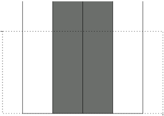
Figure 1: The situation where $k$ and $a$ are real: In (a), the shaded region denotes the part of the $UV$-plane which is mapped to the upper half plane. The tile including the origin from (a) is enlarged (and plotted with dashed lines) in (b). Here, the shaded region denotes the image of the local coordinate patch under the map $z\mapsto a\tan^{-1}z$; condition (iii) demands that it fits into the dashed tile.

Case 1: $k$, $a$ real. Since $\tan^{-1}$ maps the unit upper half disk into the region $|\text{Re }Z|\leq\frac{\pi}{4}$, $\text{Im }Z\geq 0$, property (iii) requires that $\frac{1}{a}\operatorname{sn}(aZ,k)$ maps this region into the upper half plane again. Using eqs. (A.27), (A.18), (A.19) and (A.20) as well as $U:=\text{Re }aZ$, $V:=\text{Im }aZ$, we derive that

$$\frac{1}{a}\operatorname{sn}(U+\text{i}V)=\frac{1}{a}\frac{\operatorname{sn}(U,k)\operatorname{dn}(V,k^{\prime})+\text{i}\operatorname{sn}(V,k^{\prime})\operatorname{cn}(V,k^{\prime})\operatorname{cn}(U,k)\operatorname{dn}(U,k)}{\operatorname{cn}^{2}(V,k^{\prime})+k^{2}\operatorname{sn}^{2}(V,k^{\prime})\operatorname{sn}^{2}(U,k)}\,.$$ (4.3)

Here, $k^{\prime}=\sqrt{1-k^{2}}$ denotes the complementary modulus. By inspection of (4.3), we find that the function on the left-hand side has positive imaginary part for $\operatorname{sn}(V,k^{\prime})\operatorname{cn}(V,k^{\prime})\operatorname{cn}(U,k)\operatorname{dn}(U,k)\geq 0$, i. e., $U\in[(2m-1)K,(2m+1)K]$ and $V\in[(m+2n)K^{\prime},(m+2n+1)K^{\prime}]$. The situation is illustrated in figure 1(a). Obviously, property (iii) here leads to the requirement that

$$K\geq\frac{a\pi}{4}\,,\qquad K^{\prime}=\infty\,.$$ (4.4)

The second condition in (4.4) fixes $k=0$, then, the first requires $a\in[0,2]$. For $k=0$, the Jacobi sine reduces to the ordinary sine function; therefore, this is the butterfly family with

$$f(z)=\frac{1}{a}\sin(a\tan^{-1}z)\qquad\text{with }a\in[0,2]\,.$$ (4.5)

In particular, it contains the sliver state with $f(z)=\tan^{-1}z$ for $a=0$, the butterfly state with $f(z)=\frac{z}{\sqrt{1+z^{2}}}$ for $a=1$, and the nothing state with $f(z)=\frac{z}{1+z^{2}}$ for $a=2$. Condition (iv) is automatically satisfied.

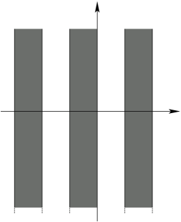
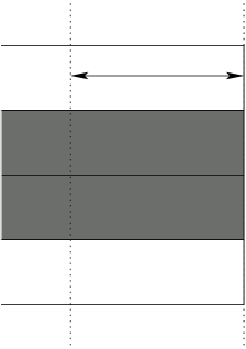
Figure 2: The situation where $k$ is real and $a$ is imaginary: In (a), the shaded region denotes the part of the $UV$-plane that is mapped to the upper half plane. The tile including the origin from (a) is enlarged (and plotted with dashed lines) in (b). Here, the shaded region denotes the image of the local coordinate patch under the map $z\mapsto a\tan^{-1}z$.

Case 2: $k$ real, $a$ imaginary. Again, we start with condition (iii). For the analysis of this case, we can recycle eq. (4.3). It is easy to see that $F(Z)$ maps the region where $\operatorname{sn}(U,k)\operatorname{dn}(V,k^{\prime})\leq 0$ to the upper half plane. This region is depicted in figure 2(a). Denoting $a=\text{i}a_{0}$ with $a_{0}$ real, we see that $Z=\frac{1}{a_{0}}(V-\text{i}U)$, i. e. the positive imaginary half-axis of $Z$ extends along the negative $U$-axis in figure 2. We read off that

$$K=\infty\qquad\Rightarrow\qquad k=1\,.$$ (4.6)

For $k=1$, the Jacobi sine reduces to the $\tanh$-function, so that the solution may be rewritten as

$$f(z)=\frac{1}{a_{0}}\tan(a_{0}\tan^{-1}z)\qquad\text{with }a_{0}\in[0,2]\,.$$ (4.7)

For $a_{0}=\frac{2}{n}$ with $n\in\mathbbm{N}$, this defines the customary wedge states, including the sliver state for $a_{0}=0$ and the identity state for $a_{0}=2$ with $f(z)=\frac{z}{1-z^{2}}$. We have bounded $a_{0}$ from above in order to ensure condition (iv); for $a_{0}\nearrow 2$, the image of the unit disk already fills the upper half plane; for $a_{0}>2$, the map is no langer one-to-one.

Case 3: $k$ imaginary, $a$ real. We first scrutinize condition (iii). An imaginary value of the elliptic modulus, $k=\text{i}k_{0}$, can be mapped to a real value $\tilde{k}:=k_{0}/\sqrt{1+k_{0}^{2}}\in[0,1)$. Introducing the abbreviations $\tilde{a}:=\sqrt{1+k_{0}^{2}}\,a$, $\tilde{k}^{\prime}:=\sqrt{1-\tilde{k}^{2}}=1/\sqrt{1+k_{0}^{2}}$, $\widetilde{U}:=\text{Re }\tilde{a}Z$, and $\widetilde{V}:=\text{Im }\tilde{a}Z$, we can use eqs. (A.24), (A.27), and (A.29) to find the following decomposition of $f(z)$ into real and imaginary parts:

$$\begin{split}F(Z)=&\,\frac{1}{\tilde{a}}\,g(\widetilde{U},\widetilde{V},\tilde{k})\,\big{(}\operatorname{sn}(\widetilde{U},\tilde{k})\operatorname{dn}(\widetilde{V},\tilde{k}^{\prime})+\text{i}\operatorname{cn}(\widetilde{U},\tilde{k})\operatorname{dn}(\widetilde{U},\tilde{k})\operatorname{sn}(\widetilde{V},\tilde{k}^{\prime})\operatorname{cn}(\widetilde{V},\tilde{k}^{\prime})\big{)}\\ &\times\big{(}\operatorname{dn}(\widetilde{U},\tilde{k})\operatorname{cn}(\widetilde{V},\tilde{k}^{\prime})\operatorname{dn}(\widetilde{V},\tilde{k}^{\prime})+\text{i}\tilde{k}^{2}\operatorname{sn}(\widetilde{U},\tilde{k})\operatorname{cn}(\widetilde{U},\tilde{k})\operatorname{sn}(\widetilde{V},\tilde{k}^{\prime})\big{)}\end{split}$$ (4.8)

with some real and positive definite function $g(\widetilde{U},\widetilde{V},\tilde{k})$. For real $a$, the imaginary part is positive exactly where $\operatorname{cn}(\widetilde{U},\tilde{k})\operatorname{sn}(\widetilde{V},\tilde{k}^{\prime})\operatorname{dn}(\widetilde{V},\tilde{k}^{\prime})$ is positive. This region is depicted in figure 3(a). Just as above, one can read off that

$$\widetilde{K}:=K(\tilde{k})\geq\frac{a\pi}{4}\,,\qquad\widetilde{K}^{\prime}:=K(\tilde{k}^{\prime})=\infty\,.$$ (4.9)

The latter condition fixes $k=0$ which was already dealt with in case 1. There are no new solutions in this situation.

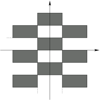
Figure 3: The situation where $k$ is imaginary: In (a), $a$ is real; the shaded region denotes the part of the $UV$-plane that is mapped to the upper half plane. In (b), $a$ is imaginary; the meaning of the shaded region is as in (a).

Case 4: $k$, $a$ imaginary. With the same notation as above, we may read off from eq. (4.8) that the imaginary part of $F(Z)$ is positive exactly where

$$\operatorname{sn}(\widetilde{U},\tilde{k})\operatorname{dn}(\widetilde{U},\tilde{k})\operatorname{cn}(\widetilde{V},\tilde{k}^{\prime})\big{(}-\operatorname{dn}^{2}(\widetilde{V},\tilde{k}^{\prime})+\tilde{k}^{2}\operatorname{cn}^{2}(\widetilde{U},\tilde{k})\operatorname{sn}^{2}(\widetilde{V},\tilde{k}^{\prime})\big{)}\geq 0\,.$$ (4.10)

Due to eqs. (A.30)–(A.32), the expression in brackets equals $-\tilde{k}^{2}\operatorname{sn}^{2}(\widetilde{U},\tilde{k})-\operatorname{dn}^{2}(\widetilde{U},\tilde{k})\operatorname{cn}^{2}(\widetilde{V},\tilde{k}^{\prime})$. Thus, $F(Z)$ maps the region where $\operatorname{sn}(\widetilde{U},\tilde{k})\operatorname{dn}(\widetilde{U},\tilde{k})\operatorname{cn}(\widetilde{V},\tilde{k}^{\prime})\leq 0$ to the upper half plane. This situation is illustrated in figure 3(b); obviously, there are no values of $\tilde{k}$ such that $f(z)$ maps the unit upper half disk completely into the upper half plane again.

Case 5: $a\in\mathbbm{C}\backslash\{0\}$, $k=\pm{\bar{a}}/a$. The last case is the situation where $k$ takes values in the unit circle. The analysis in this case is a slightly more involved than before. We restrict the discussion to the case $k=\frac{{\bar{a}}}{a}$; the other case with $k=-\frac{{\bar{a}}}{a}$ can be treated analogously. We already saw in eqs. (4.1) and (4.2) that with $k=\pm{\bar{a}}/a$,

$$\frac{1}{a}\operatorname{sn}\big{(}aX,{\textstyle\frac{{\bar{a}}}{a}}\big{)}\in\mathbbm{R}$$ (4.11)

for $X\in\mathbbm{R}$; similarly, it is trivial to see that

$$\frac{1}{a}\operatorname{sn}\big{(}\text{i}aY,{\textstyle\frac{{\bar{a}}}{a}}\big{)}\in\text{i}\,\mathbbm{R}$$ (4.12)

for $Y\in\mathbbm{R}$. Since furthermore, for $k=1$, $\operatorname{cn}(u,k)=\overline{\operatorname{dn}(u,k)}$, eq. (A.27) yields the following imaginary part:

$$\text{Im }\frac{1}{a}\operatorname{sn}\big{(}a(X+\text{i}Y)\big{)}=\frac{-{\textstyle\frac{\text{i}}{a}}\operatorname{sn}(\text{i}aY)|\operatorname{cn}(aX)|^{2}}{1-{\textstyle\frac{|a|^{4}}{a^{4}}}\operatorname{sn}^{2}(aX)\operatorname{sn}^{2}(\text{i}aY)}\,,$$ (4.13)

where the elliptic modulus is always ${\textstyle\frac{{\bar{a}}}{a}}$. Because of (4.11) and (4.12), the denominator is positive; thus, the imaginary part is positive exactly where $-{\textstyle\frac{\text{i}}{a}}\operatorname{sn}(\text{i}aY)$ is. A careful analysis using the zeroes and singularities given in appendix A and the conjugation properties (A.9) and (A.10) shows that the singularities of the Jacobi sine function bound the real values of $Y$ for which the imaginary part of $-{\textstyle\frac{\text{i}}{a}}\operatorname{sn}(\text{i}aY)$ is positive. The intervals for which this is so are (for $k=\text{e}^{\text{i}\alpha}$):

$$-\frac{\text{i}}{a}\operatorname{sn}(\text{i}aY)\geq 0\qquad\text{for }\begin{cases}Y\in[0,\frac{1}{a}K^{\prime})&\text{if }-\frac{\pi}{2}<\alpha<\frac{\pi}{2}\,,\\ Y\in[0,\frac{2}{\text{i}a}K+\frac{1}{a}K^{\prime})&\text{if }\frac{\pi}{2}<\alpha<\pi\,,\\ Y\in[0,\frac{2}{\text{i}a}K-\frac{1}{a}K^{\prime})&\text{if }\pi<\alpha<\frac{3\pi}{2}\,.\end{cases}$$ (4.14)

As above, the elliptic modulus is always ${\textstyle\frac{{\bar{a}}}{a}}$. Since condition (iii) requires the upper bound of these intervals to be infinite this case only leads (asymptotically) to the solution $k=\text{e}^{\text{i}\pi}=-1$ (i. e., the sliver, which was already discussed in case 1).

This concludes the proof that there are no twist-even $\kappa$-diagonal surface states apart from the butterfly family (4.5) and a trivial extension of the wedge states admitting arbitrary angles, cf. eq. (4.7).

5 Conclusions

In this paper, we have derived and analyzed a consistency condition on twist-even $\kappa$-diagonal surface states. The general solution was found to be a two-parameter family of (candidate) maps defining a surface state, $\frac{1}{a}\operatorname{sn}(a\tan^{-1}z,k)$. This family contains the well-known butterfly family as well as an extension of the family of wedge states to arbitrary angles; and the conditions that the meromorphic function $f(z)$ map the real line to itself and the unit upper half disk one-to-one to some region of the upper half plane were enough to show that these are in fact the only admissible maps to define a surface state.

In particular, this result demonstrates that surface state projectors which do not satisfy the sufficient condition that their boundary touches the midpoint of the open string (i. e., $f(\text{i})=\infty$ in upper half plane coordinates) are particularly rare – at least in the subsector of twist-even $\kappa$-diagonal surface state projectors, we only found the identity state. All other projectors share this singular property.

Furthermore, this result completes the classification of $\kappa$-diagonal projectors (in a fermionic first order system) commenced in [19]. Besides, it also proves the conjecture made in [22] that the projectors $P_{2m}$ defined by $f(z)=z(1-(-z^{2})^{m})^{-1/2m}$ for $m>1$ are not contained in the ${\cal H}_{\kappa^{2}}$ subalgebra. Hitherto, this conjecture had only been checked numerically.

It is conceivable that the strategy pursued here can be extended to the general case without the restriction to the twist-even subsector. The hope that underlies this approach is that a better knowledge of the algebraic structures of the star algebra will help to pave the way to solving the equation of motion of string field theory.

Acknowledgements

I would like to thank Alexander Kling, Yuji Okawa, Martin Schnabl, Wati Taylor, David Tong, and Barton Zwiebach for discussions. Furthermore, I would like to thank Matthias Ihl for encouragement as well as a collaboration at an intermediate stage. This work was supported by a fellowship within the postdoc program of the German Academic Exchange Service (DAAD).

Appendix A Jacobian elliptic functions

In this appendix, we present the definitions and properties of the Jacobian elliptic functions used throughout the text. A good reference for some of the formulas is [33].

Definitions. The Jacobian elliptic functions (of which we need here only $\operatorname{sn}$, $\operatorname{cn}$, and $\operatorname{dn}$) are doubly-periodic functions defined as the (analytic continuation of the) inverse of elliptic integrals,

$$u =\int_{0}^{\operatorname{sn}u}\frac{dt}{\sqrt{(1-t^{2})(1-k^{2}t^{2})}}\,,$$ (A.1)

$$u =\int_{1}^{\operatorname{cn}u}\frac{dt}{\sqrt{(1-t^{2})(k^{\prime 2}-k^{2}t^{2})}}\,,$$ (A.2)

$$u =\int_{1}^{\operatorname{dn}u}\frac{dt}{\sqrt{(1-t^{2})(t^{2}-k^{\prime 2})}}\,.$$ (A.3)

Here, $k$ denotes the modulus, $k^{\prime}=\sqrt{1-k^{2}}$ is the complementary modulus. Note that a number of incompatible conventions for the modulus are in common use, e. g., $k$ is often replaced by its square. If the modulus is obvious, it is mostly omitted (as above); otherwise, we denote it explicitly by $\operatorname{sn}(u,k)$ etc. For $k=0$, $\operatorname{sn}$ and $\operatorname{cn}$ reduce to the ordinary trigonometric functions, $\operatorname{sn}(u,0)=\sin u$ and $\operatorname{cn}(u,0)=\cos u$ (and $\operatorname{dn}(u,0)=1$). For $k=1$, $\operatorname{sn}(u,1)=\tanh u$ and $\operatorname{cn}(u,1)=\operatorname{dn}(u,1)=\text{sech }u$.

Complete elliptic integrals. The periodicity and zeroes of the Jacobian elliptic functions can be expressed in terms of the complete elliptic integral of the first kind,

$$K:=K(k)=\int_{0}^{1}\frac{dx}{\sqrt{(1-x^{2})(1-k^{2}x^{2})}}\,,$$ (A.4)

where the modulus $k$ is often omitted. This is the value $u$ where the Jacobi sine function equals 1. It is customary to set

$$K^{\prime}:=K(k^{\prime})\,.$$ (A.5)

In general, we have

$$\overline{K(k)}=K(\bar{k})\,,\qquad\overline{K^{\prime}(k)}=K^{\prime}(\bar{k})\,,$$ (A.6)

where the bar denotes complex conjugation. This ensures that the period parallelogram of the Jacobian elliptic functions specified in the next paragraph is a rectangle. The elliptic integral of the first kind has a branch cut from 1 to $\infty$.

Particular values are $K(0)=\frac{\pi}{2}$ and $K(1)=\infty$. For the analysis in section 4, we derive some further properties for $|k|=1$: Setting $k=\text{e}^{\text{i}\alpha}=\frac{{\bar{a}}}{a}$ and being careful with the branchcuts, we can check that

$$K^{\prime}\big{(}{\textstyle\frac{1}{k}}\big{)}=\begin{cases}k\,K^{\prime}(k)&\text{for }-\frac{\pi}{2}<\alpha<\frac{\pi}{2}\,,\\ -k\,K^{\prime}(k)&\text{for }\frac{\pi}{2}<\alpha<\frac{3\pi}{2}\,,\\ \end{cases}$$ (A.7)

and

$$K\big{(}{\textstyle\frac{1}{k}}\big{)}=\begin{cases}k(K(k)-\text{i}K^{\prime}(k))&\text{for }0<\alpha<\frac{\pi}{2}\,,\\ -k(K(k)+\text{i}K^{\prime}(k))&\text{for }\frac{\pi}{2}<\alpha<\pi\,,\\ -k(K(k)-\text{i}K^{\prime}(k))&\text{for }\pi<\alpha<\frac{3\pi}{2}\,,\\ k(K(k)+\text{i}K^{\prime}(k))&\text{for }\frac{3\pi}{2}<\alpha<2\pi\,.\end{cases}$$ (A.8)

Therefore, we obtain the conjugation properties

$$\overline{\frac{1}{a}K^{\prime}(k)}=\frac{1}{{\bar{a}}}K^{\prime}\big{(}{\textstyle\frac{1}{k}}\big{)}\begin{cases}\frac{1}{a}K^{\prime}(k)&\text{for }-\frac{\pi}{2}<\alpha<\frac{\pi}{2}\,,\\ -\frac{1}{a}K^{\prime}(k)&\text{for }\frac{\pi}{2}<\alpha<\frac{3\pi}{2}\end{cases}$$ (A.9)

and

$$\overline{\frac{1}{\text{i}a}K(k)}=-\frac{1}{\text{i}a}K\big{(}{\textstyle\frac{1}{k}}\big{)}=\begin{cases}-\frac{1}{\text{i}a}K(k)+\frac{1}{a}K^{\prime}(k)&\text{for }0<\alpha<\frac{\pi}{2}\,,\\ \frac{1}{\text{i}a}K(k)+\frac{1}{a}K^{\prime}(k)&\text{for }\frac{\pi}{2}<\alpha<\pi\,,\\ \frac{1}{\text{i}a}K(k)-\frac{1}{a}K^{\prime}(k)&\text{for }\pi<\alpha<\frac{3\pi}{2}\,,\\ -\frac{1}{\text{i}a}K(k)-\frac{1}{a}K^{\prime}(k)&\text{for }\frac{3\pi}{2}<\alpha<2\pi\,.\end{cases}$$ (A.10)

Symmetries, periodicities, zeroes, and poles. The Jacobi sine function is an odd function of its first argument, the Jacobi cosine function as well as the delta function are even w. r. t. to $u$. All three functions are even in $k$. For $|u|<K^{\prime}$, the power series expansion takes the form:

$$\operatorname{sn}u =u-\frac{1+k^{2}}{3!}u^{3}+\frac{1+14k^{2}+k^{4}}{5!}u^{5}-\frac{1+135k^{2}+135k^{4}+k^{6}}{7!}u^{7}+\ldots\,,$$ (A.11)

$$\operatorname{cn}u =1-\frac{1}{2!}u^{2}+\frac{1+4k^{2}}{4!}u^{4}-\frac{1+44k^{2}+16k^{4}}{6!}u^{6}+\ldots\,,$$ (A.12)

$$\operatorname{dn}u =1-\frac{k^{2}}{2!}u^{2}+\frac{k^{2}(4+k^{2})}{4!}u^{4}-\frac{k^{2}(16+44k^{2}+k^{4})}{6!}u^{6}+\ldots\,.$$ (A.13)

A closed form for the Taylor coefficients is unknown. The Jacobian elliptic functions are not periodic in $k$; the periods, zeroes, and poles in $u$ are located at:

	Periods	Zeroes	Poles
$\operatorname{sn}u$	$4mK+2nK^{\prime}\text{i}$	$2mK+2nK^{\prime}\text{i}$	$2mK+(2n+1)K^{\prime}\text{i}$
$\operatorname{cn}u$	$4mK+2n(K+K^{\prime}\text{i})$	$(2m+1)K+2nK^{\prime}\text{i}$	$2mK+(2n+1)K^{\prime}\text{i}$
$\operatorname{dn}u$	$2mK+4nK^{\prime}\text{i}$	$(2m+1)K+(2n+1)K^{\prime}\text{i}$	$2mK+(2n+1)K^{\prime}\text{i}$

Here, it is understood that $m,n\in\mathbbm{Z}$. One can read off from

$$\operatorname{sn}(u+2mK+2nK^{\prime}\text{i},k) =(-1)^{m}\operatorname{sn}(u,k)\,,$$ (A.14)

$$\operatorname{cn}(u+2mK+2nK^{\prime}\text{i},k) =(-1)^{m+n}\operatorname{cn}(u,k)\,,$$ (A.15)

$$\operatorname{dn}(u+2mK+2nK^{\prime}\text{i},k) =(-1)^{n}\operatorname{dn}(u,k)\,,$$ (A.16)

and $\operatorname{sn}(0,k)=0$, $\operatorname{cn}(K,k)=0$ that the Jacobi sine function changes sign only along the real axis whereas the Jacobi cosine function does so along both axes.

In general, we have

$$\overline{\operatorname{sn}(u,k)}=\operatorname{sn}(\bar{u},\bar{k})\,,\quad\overline{\operatorname{cn}(u,k)}=\operatorname{cn}(\bar{u},\bar{k})\,,\quad\overline{\operatorname{dn}(u,k)}=\operatorname{dn}(\bar{u},\bar{k})\,.$$ (A.17)

For $|k|=1$, $\operatorname{cn}$ and $\operatorname{dn}$ are complex conjugate to each other in the sense that $\operatorname{cn}(u,k)=\overline{\operatorname{dn}(u,k)}$.

Useful formulas. In order to check which parts of the complex plane are mapped to the upper half plane, we need the following useful identities:

$$\operatorname{sn}(\text{i}u,k) =\text{i}\frac{\operatorname{sn}(u,k^{\prime})}{\operatorname{cn}(u,k^{\prime})}\,,$$ (A.18)

$$\operatorname{cn}(\text{i}u,k) =\frac{1}{\operatorname{cn}(u,k^{\prime})}\,,$$ (A.19)

$$\operatorname{dn}(\text{i}u,k) =\frac{\operatorname{dn}(u,k^{\prime})}{\operatorname{cn}(u,k^{\prime})}$$ (A.20)

as well as

$$\operatorname{sn}(u,k) =k^{-1}\operatorname{sn}(ku,k^{-1})\,,$$ (A.21)

$$\operatorname{cn}(u,k) =\operatorname{dn}(ku,k^{-1})\,,$$ (A.22)

$$\operatorname{dn}(u,k) =\operatorname{cn}(ku,k^{-1})$$ (A.23)

and

$$\operatorname{sn}(u,\text{i}k) =\frac{1}{\sqrt{1+k^{2}}}\frac{\operatorname{sn}(\sqrt{1+k^{2}}u,k/\sqrt{1+k^{2}})}{\operatorname{dn}(\sqrt{1+k^{2}}u,k/\sqrt{1+k^{2}})}\,,$$ (A.24)

$$\operatorname{cn}(u,\text{i}k) =\frac{\operatorname{sn}(\sqrt{1+k^{2}}u,k/\sqrt{1+k^{2}})}{\operatorname{dn}(\sqrt{1+k^{2}}u,k/\sqrt{1+k^{2}})}\,,$$ (A.25)

$$\operatorname{dn}(u,\text{i}k) =\frac{1}{\operatorname{dn}(\sqrt{1+k^{2}}u,k/\sqrt{1+k^{2}})}\,.$$ (A.26)

Addition formulas. In analogy to the addition formulas for the trigonometric functions, we have:

$$\operatorname{sn}(u\pm v) =\frac{\operatorname{sn}u\operatorname{cn}v\operatorname{dn}v\pm\operatorname{sn}v\operatorname{cn}u\operatorname{dn}u}{1-k^{2}\operatorname{sn}^{2}u\operatorname{sn}^{2}v}\,,$$ (A.27)

$$\operatorname{cn}(u\pm v) =\frac{\operatorname{cn}u\operatorname{cn}v\mp\operatorname{sn}u\operatorname{sn}v\operatorname{dn}u\operatorname{dn}u}{1-k^{2}\operatorname{sn}^{2}u\operatorname{sn}^{2}v}\,,$$ (A.28)

$$\operatorname{dn}(u\pm v) =\frac{\operatorname{dn}u\operatorname{dn}v\mp k^{2}\operatorname{sn}u\operatorname{sn}v\operatorname{cn}u\operatorname{cn}v}{1-k^{2}\operatorname{sn}^{2}u\operatorname{sn}^{2}v}\,.$$ (A.29)

Relation among the elliptic functions. The Jacobian elliptic functions are related by:

$$\operatorname{sn}^{2}u+\operatorname{cn}^{2}u =1\,,$$ (A.30)

$$k^{2}\operatorname{sn}^{2}u+\operatorname{dn}^{2}u =1\,,$$ (A.31)

$$k^{2}\operatorname{cn}^{2}u+k^{\prime 2} =\operatorname{dn}^{2}u\,,$$ (A.32)

$$\operatorname{cn}^{2}u+k^{\prime 2}\operatorname{sn}^{2}u =\operatorname{dn}^{2}u\,.$$ (A.33)

References

- [1] W. Taylor and B. Zwiebach, D-branes, tachyons, and string field theory, arXiv:hep-th/0311017.
- [2] E. Witten, Noncommutative geometry and string field theory, Nucl. Phys. B 268 (1986) 253.
- [3] L. Rastelli, A. Sen and B. Zwiebach, String field theory around the tachyon vacuum, Adv. Theor. Math. Phys. 5 (2002) 353 [arXiv:hep-th/0012251].
- [4] L. Rastelli, A. Sen and B. Zwiebach, Classical solutions in string field theory around the tachyon vacuum, Adv. Theor. Math. Phys. 5 (2002) 393 [arXiv:hep-th/0102112].
- [5] H. Hata and T. Kawano, Open string states around a classical solution in vacuum string field theory, JHEP 0111 (2001) 038 [arXiv:hep-th/0108150].
- [6] D. Gaiotto, L. Rastelli, A. Sen and B. Zwiebach, Ghost structure and closed strings in vacuum string field theory, Adv. Theor. Math. Phys. 6 (2003) 403 [arXiv:hep-th/0111129].
- [7] K. Okuyama, Ghost kinetic operator of vacuum string field theory, JHEP 0201 (2002) 027 [arXiv:hep-th/0201015];
- [8] D. J. Gross and A. Jevicki, Operator formulation of interacting string field theory, Nucl. Phys. B 283 (1987) 1.
- [9] D. J. Gross and A. Jevicki, Operator formulation of interacting string field theory. 2, Nucl. Phys. B 287 (1987) 225.
- [10] M. R. Douglas, H. Liu, G. Moore and B. Zwiebach, Open string star as a continuous Moyal product, JHEP 0204 (2002) 022 [arXiv:hep-th/0202087].
- [11] D. M. Belov, Diagonal representation of open string star and Moyal product, arXiv:hep-th/0204164.
- [12] I. Ya. Aref’eva and A. A. Giryavets, Open superstring star as a continuous Moyal product, JHEP 0212 (2002) 074 [arXiv:hep-th/0204239].
- [13] T. G. Erler, Moyal formulation of Witten’s star product in the fermionic ghost sector, arXiv:hep-th/0205107.
- [14] D. M. Belov and A. Konechny, On continuous Moyal product structure in string field theory, JHEP 0210 (2002) 049 [arXiv:hep-th/0207174].
- [15] D. M. Belov and C. Lovelace, Witten’s vertex made simple, Phys. Rev. D 68 (2003) 066003 [arXiv:hep-th/0304158];
- [16] D. M. Belov, Witten’s ghost vertex made simple (bc and bosonized ghosts), Phys. Rev. D 69 (2004) 126001 [arXiv:hep-th/0308147].
- [17] C. Maccaferri and D. Mamone, Star democracy in open string field theory, JHEP 0309 (2003) 049 [arXiv:hep-th/0306252].
- [18] A. Kling and S. Uhlmann, String field theory vertices for fermions of integral weight, JHEP 0307 (2003) 061 [arXiv:hep-th/0306254].
- [19] M. Ihl, A. Kling and S. Uhlmann, String field theory projectors for fermions of integral weight, JHEP 0403 (2004) 002 [arXiv:hep-th/0312314].
- [20] I. Bars, Map of Witten’s * to Moyal’s *, Phys. Lett. B 517 (2001) 436 [arXiv:hep-th/0106157].
- [21] I. Bars and Y. Matsuo, Computing in string field theory using the Moyal star product, Phys. Rev. D 66 (2002) 066003 [arXiv:hep-th/0204260].
- [22] E. Fuchs, M. Kroyter and A. Marcus, Squeezed state projectors in string field theory, JHEP 0209 (2002) 022 [arXiv:hep-th/0207001].
- [23] O. Lechtenfeld, A. D. Popov and S. Uhlmann, Exact solutions of Berkovits’ string field theory, Nucl. Phys. B 637 (2002) 119 [arXiv:hep-th/0204155].
- [24] A. Kling, O. Lechtenfeld, A. D. Popov and S. Uhlmann, On nonperturbative solutions of superstring field theory, Phys. Lett. B 551 (2003) 193 [arXiv:hep-th/0209186].
- [25] A. Kling, O. Lechtenfeld, A. D. Popov and S. Uhlmann, Solving string field equations: New uses for old tools, Fortschr. Phys. 51 (2003) 775 [arXiv:hep-th/0212335].
- [26] A. LeClair, M. E. Peskin and C. R. Preitschopf, String field theory on the conformal plane. 1. Kinematical principles, Nucl. Phys. B 317 (1989) 411.
- [27] A. LeClair, M. E. Peskin and C. R. Preitschopf, String field theory on the conformal plane. 2. Generalized gluing, Nucl. Phys. B 317 (1989) 464.
- [28] D. Gaiotto, L. Rastelli, A. Sen and B. Zwiebach, Star algebra projectors, JHEP 0204 (2002) 060 [arXiv:hep-th/0202151].
- [29] T. Okuda, The equality of solutions in vacuum string field theory, Nucl. Phys. B 641 (2002) 393 [arXiv:hep-th/0201149].
- [30] I. Bars, I. Kishimoto and Y. Matsuo, Fermionic ghosts in Moyal string field theory, JHEP 0307 (2003) 027 [arXiv:hep-th/0304005].
- [31] M. Schnabl, Anomalous reparametrizations and butterfly states in string field theory, Nucl. Phys. B 649 (2003) 101 [arXiv:hep-th/0202139].
- [32] L. Rastelli, A. Sen and B. Zwiebach, Vacuum string field theory, arXiv:hep-th/0106010.
- [33] I. S. Gradshteyn, I. M. Ryzhik, Table of integrals, series, and products, 6th edition, Academic Press (2000), sections 8.11-8.15.