Matrix Factorizations And Mirror Symmetry: The Cubic Curve

CERN–PH–TH/2004-162 KCL-MTH-04-12 NSF-KITP-04-106 hep-th/0408243

August 2004

1 Introduction

The considerable recent progress in computing non-perturbative superpotentials (and other holomorphic quantities) in $N=1$ string vacua, has left behind several open questions concerning the general systematics of open topological strings [1]. The list includes, on the technical side, the proper inclusion of boundary changing sectors, associated with worldsheets spanning between different branes. On the conceptual side, it remains an outstanding question how to find, in general, proper ”special coordinates” of mirror symmetry on the combined open-closed string parameter space. This latter problem is severe not only if boundary changing sectors are included, but even more so when deformations are obstructed and the notion of flatness becomes an off-shell or merely infinitesimal question.

Recently, a promising approach for describing topological $D$-branes in the $B$-model has been developped which is based on boundary Landau-Ginzburg theory [2, 3, 4, 5, 6, 7, 8, 9, 10, 11], building on previous work [12, 13, 14, 15, 16] and [17, 18]. It seems to capture all the relevant information about the category of topological $D$-branes of $B$-type, and has been successfully applied in particular to the topological minimal models, for which the complete effective superpotential on the disk has been determined [9]. This was achieved by solving the open string version [19] of the WDVV equations, which include the $A_{\infty}$ relations. Moreover, the formulas for topological correlators given in [4, 10], as well as the concrete study of the problem’s deformation theory [8, 7], have given valuable pieces of information about the above questions also in more geometrical settings.

In the present paper, we study these problems for the simplest model that has a compact geometric interpretation, namely the cubic elliptic curve. The representation of its $B$-type branes in terms of matrix factorizations in the Landau-Ginzburg model has recently been discussed in [8]. It is based on the superpotential

$$W(x,{a})\ =\ \frac{1}{3}{x_{1}}^{3}+\frac{1}{3}{x_{2}}^{3}+\frac{1}{3}{x_{3}}^{3}-{a}\,x_{1}x_{2}x_{3}\,,$$ (1)

together with an obvious ${\mathbb{Z}}_{3}$ orbifold action. This model corresponds to the point $\rho=\exp{2\pi{\rm i}/3}$ in Kähler moduli space, and the complex structure parameter varies as a certain function $\tau=\tau({a})$. On the physics side, this model is exactly solvable at the CFT level. On the mathematical side, the elliptic curve has been studied extensively from the point of view of categorical mirror symmetry in [20, 21, 22, 23, 24, 1], so that most of the questions we might want to ask should have known answers. Our goal here is to learn how to derive some of these results from the boundary Landau-Ginzburg realization, with the expectation that the lessons we learn will be useful in more complicated situations.

Specifically, we will focus on the computation of the effective “Yukawa” couplings associated with pairwise intersections of three branes. When expressed in flat coordinates, which we determine intrinsically in the $B$-model, these Yukawa couplings become the $A$-model generating functions for triangle-shaped world-sheet instantons that span between the three $D$-branes. From the point of view of categorical mirror symmetry, our results amount to determining the associative Fukaya products $m_{2}$ from their Landau-Ginzburg $B$-model counterparts. The computation of the higher, non-associative products $m_{k}$ will be addressed elsewhere.

2 $D$-branes, matrix factorizations and $Q$-cohomology

As discussed in [8], the $B$-type $D$-branes of this model can be obtained from all possible matrix factorizations of (1). For $a=0$, those factorizations have been put in exact correspondence [25] with vector bundles on the elliptic curve $W=0\subset{\mathbb{P}}^{2}$, which were classified by Atiyah. Simplest are the ${\mathbb{Z}}_{3}$-equivariant $3\times 3$ factorizations involving the boundary BRST operators [8]

$$Q_{i}=\begin{pmatrix}0&J_{i}\\ E_{i}&0\end{pmatrix}\ ,\qquad i=1,2,3\ ,$$ (2)

with

$$\begin{split}J_{i}&=\begin{pmatrix}{{\alpha_{1}^{i}}}{x_{1}}&{{\alpha_{2}^{i}}}{x_{3}}&{{\alpha_{3}^{i}}}{x_{2}}\\ {{\alpha_{3}^{i}}}{x_{3}}&{{\alpha_{1}^{i}}}{x_{2}}&{{\alpha_{2}^{i}}}{x_{1}}\\ {{\alpha_{2}^{i}}}{x_{2}}&{{\alpha_{3}^{i}}}{x_{1}}&{{\alpha_{1}^{i}}}{x_{3}}\end{pmatrix}\\ E_{i}&=\begin{pmatrix}\frac{1}{{{\alpha_{1}^{i}}}}{x_{1}}^{2}-\frac{{{\alpha_{1}^{i}}}}{{{\alpha_{2}^{i}}}{{\alpha_{3}^{i}}}}{x_{2}}{x_{3}}&\frac{1}{{{\alpha_{3}^{i}}}}{x_{3}}^{2}-\frac{{{\alpha_{3}^{i}}}}{{{\alpha_{1}^{i}}}{{\alpha_{2}^{i}}}}{x_{1}}{x_{2}}&\frac{1}{{{\alpha_{2}^{i}}}}{x_{2}}^{2}-\frac{{{\alpha_{2}^{i}}}}{{{\alpha_{1}^{i}}}{{\alpha_{3}^{i}}}}{x_{1}}{x_{3}}\\ \frac{1}{{{\alpha_{2}^{i}}}}{x_{3}}^{2}-\frac{{{\alpha_{2}^{i}}}}{{{\alpha_{1}^{i}}}{{\alpha_{3}^{i}}}}{x_{1}}{x_{2}}&\frac{1}{{{\alpha_{1}^{i}}}}{x_{2}}^{2}-\frac{{{\alpha_{1}^{i}}}}{{{\alpha_{2}^{i}}}{{\alpha_{3}^{i}}}}{x_{1}}{x_{3}}&\frac{1}{{{\alpha_{3}^{i}}}}{x_{1}}^{2}-\frac{{{\alpha_{3}^{i}}}}{{{\alpha_{1}^{i}}}{{\alpha_{2}^{i}}}}{x_{2}}{x_{3}}\\ \frac{1}{{{\alpha_{3}^{i}}}}{x_{2}}^{2}-\frac{{{\alpha_{3}^{i}}}}{{{\alpha_{1}^{i}}}{{\alpha_{2}^{i}}}}{x_{1}}{x_{3}}&\frac{1}{{{\alpha_{2}^{i}}}}{x_{1}}^{2}-\frac{{{\alpha_{2}^{i}}}}{{{\alpha_{1}^{i}}}{{\alpha_{3}^{i}}}}{x_{2}}{x_{3}}&\frac{1}{{{\alpha_{1}^{i}}}}{x_{3}}^{2}-\frac{{{\alpha_{1}^{i}}}}{{{\alpha_{2}^{i}}}{{\alpha_{3}^{i}}}}{x_{1}}{x_{2}}\end{pmatrix}\ .\end{split}$$ (3)

The ${\alpha_{\ell}^{i}}$ are parameters that are constrained by the matrix factorization condition $Q_{i}^{2}(x,{\alpha_{\ell}^{i}})=W(x,{a}){\bf 1}$, which translates to [8]:

$$\frac{1}{3}({\alpha_{1}^{i}})^{3}+\frac{1}{3}({\alpha_{2}^{i}})^{3}+\frac{1}{3}({\alpha_{3}^{i}})^{3}-{a}\,{{\alpha_{1}^{i}}}{{\alpha_{2}^{i}}}{{\alpha_{3}^{i}}}=0\,.$$ (4)

Thus, the moduli space spanned by the ${\alpha_{\ell}^{i}}$ is isomorphic to the Jacobian of the torus itself, and this is expected to hold for any matrix factorization of (1). As explained in [8], the three particular matrix factorizations based on (2), (3) describe one-parameter deformations of the rational $D$-branes, for any given value of the bulk modulus, ${a}(\tau)$. These branes, which we shall denote by ${\mathcal{L}}_{1}$, ${\mathcal{L}}_{2}$, ${\mathcal{L}}_{3}$, are known [25] to correspond, in the geometric $B$-model category, to bundles with ranks and degres given by $(r,c_{1})=(2,1),(-1,1),(-1,-2)$, respectively. In physics terms, these labels correspond to $D2$- and $D0$-brane charges, respectively (the one-parameter deformations correspond to the locations of the $D0$-branes on top of the $D2$-branes, which by themselves wrap the cubic curve). Since $r+c_{1}=0\bmod 3$ for all three branes, the ${\mathcal{L}}_{i}$ do not provide an integral basis of the complete $K$-charge lattice, which is a familiar feature in this context [26]. In the appendix, we exhibit a set of $2\times 2$ matrix factorizations of the cubic that does correspond to such an integral basis.

In the mirror description, in which (the roles of) $\rho$ and $\tau$ are exchanged, quasihomogeneous matrix factorizations correspond to branes wrapped along special Lagrangian submanifolds of the torus ${\mathbb{C}}/({\mathbb{Z}}+\rho{\mathbb{Z}})$, with wrapping numbers $(n_{1},n_{2})=(r,c_{1})$. In particular, the $A$-model mirrors of the three branes ${\mathcal{L}}_{i}$ described by (3) can be pictured as the three long diagonals of the $SU(3)$ torus, see Fig. 1. In $A$-model language, the boundary moduli correspond to position and flat gauge fields on the lines, and we will describe further below the mirror map between them and the $B$-model moduli ${a}$, ${\alpha_{\ell}^{i}}$.

Figure 1: Shown are the long and short diagonals on the covering space of the torus; note that they correspond to roots and weights of the $SU(3)$ lattice, resp. The long diagonals ${\mathcal{L}}_{i}$ correspond, via mirror symmetry, to the $3\times 3$ matrix factorizarions (3) we discuss in this paper, while the short diagonals ${\mathcal{S}}_{i}$ correspond to $2\times 2$ factorizations.

We now turn to discussing the boundary changing operators, that is, cohomology representatives of the open string spectrum between pairs of the ${\mathcal{L}}_{i}$. We have summarized the open string spectrum in the quiver diagram of Fig. 2. As indicated, in the boundary changing sector between ${\mathcal{L}}_{j}$ and ${\mathcal{L}}_{i}$ (with $i=j+1\bmod 3$) there are three bosonic and three fermionic elements, $\Phi_{ji}^{(a)}$ resp. $\Psi_{ij}^{(a)}$ ($a=1,2,3$). These correspond to the three intersection points each pair of branes has, when translated to a fundamental domain. Moreover, $\Omega_{i}$ denote boundary preserving operators of top degree (R-charge) $1$, which generate the marginal deformations of the branes. The $\Omega_{i}$ will be discussed at length in the next section.

Figure 2: Quiver representation of the open string spectrum between the three $D$-branes ${\mathcal{L}}_{i}$ under consideration. One of our objectives is to find suitable Landau-Ginzburg representatives of all the pictured quantities that continuously depend on the bulk/boundary moduli.

In order to construct LG representatives, it is useful to first determine the degrees (charges) of the open string operators. Note that (3) is quasihomogeneous with R-charge assignement

$${\rm e}^{{\rm i}\lambda R}=\begin{pmatrix}{\rm e}^{{\rm i}\lambda/6}\,{\bf 1}_{3}&0\\ 0&{\rm e}^{-{\rm i}\lambda/6}\,{\bf 1}_{3}\end{pmatrix}$$ (5)

and equivariant with respect to the following orbifold action

$${\rm e}^{2\pi j{\rm i}/3}\begin{pmatrix}{\bf 1}_{3}&0\\ 0&-{\rm e}^{-{\rm i}\pi/3}\,{\bf 1}_{3}\end{pmatrix}\qquad(j=1,2,3)$$ (6)

on the Chan-Paton spaces. Therefore, in order to survive the orbifolding, $\Phi_{ij}^{(a)}$ and $\Psi_{ij}^{(a)}$ must have R-charge $q_{\Phi}=2/3$ and $q_{\Psi}=1/3$, respectively. [Note, however, that this is subject to change once we move the Kähler modulus away from $\rho=\exp{2\pi{\rm i}/3}$. The important invariant statement is $q_{\Phi}+q_{\Psi}=1$ by charge conjugation (Serre duality), and $0<q_{\Phi}<1$ so that $\Phi$ and $\Psi$ are always tachyonic; there are no lines of marginal stability on the torus.]

We start with finding representative of the fermionic operators $\Psi_{ij}^{(a)}$ mapping from ${\mathcal{L}}_{j}$ to ${\mathcal{L}}_{i}$. We will explicitly take $i=2$ and $j=1$, but everything works analogously for $i=j+1\bmod 3$. Writing

$$\Psi_{21}=\begin{pmatrix}0&F_{21}\\ G_{21}&0\end{pmatrix}\,,$$ (7)

$Q$-closedness requires that $F$ and $G$ satisfy

$$\begin{split}J_{2}G_{21}+F_{21}E_{1}&=0\\ E_{2}F_{21}+G_{21}J_{1}&=0\end{split}$$ (8)

The above degree considerations in the orbifold dictate that $F$ be constant (i.e., independent of ${x_{\ell}}$) and $G$ be linear in ${x_{\ell}}$. One may also note that the image of the $Q_{i}$’s at this degree is zero (there are no bosonic operators in degree $-2/3$, as this would require negative powers of $x_{\ell}$), so that all solutions to (8) will be cohomologically non-trivial.

All-in-all, one indeed finds three linearly independent solutions of (8), which are precisely the $\Psi_{21}^{(a)}$ we are looking for. The first one reads

$$F^{(1)}_{21}=\begin{pmatrix}{{\zeta_{1}}}&0&0\\ 0&0&{{\zeta_{2}}}\\ 0&{{\zeta_{3}}}&0\end{pmatrix}\qquad G^{(1)}_{21}=-\begin{pmatrix}\frac{{{\zeta_{1}}}}{{{\alpha_{1}^{1}}}{{\alpha_{1}^{2}}}}{x_{1}}&\frac{{{\zeta_{3}}}}{{{\alpha_{1}^{1}}}{{\alpha_{2}^{2}}}}{x_{2}}&\frac{{{\zeta_{2}}}}{{{\alpha_{1}^{1}}}{{\alpha_{3}^{2}}}}{x_{3}}\\ \frac{{{\zeta_{2}}}}{{{\alpha_{1}^{2}}}{{\alpha_{3}^{1}}}}{x_{2}}&\frac{{{\zeta_{1}}}}{{{\alpha_{2}^{2}}}{{\alpha_{3}^{1}}}}{x_{3}}&\frac{{{\zeta_{3}}}}{{{\alpha_{3}^{1}}}{{\alpha_{3}^{2}}}}{x_{1}}\\ \frac{{{\zeta_{3}}}}{{{\alpha_{1}^{2}}}{{\alpha_{2}^{1}}}}{x_{3}}&\frac{{{\zeta_{2}}}}{{{\alpha_{2}^{1}}}{{\alpha_{2}^{2}}}}{x_{1}}&\frac{{{\zeta_{1}}}}{{{\alpha_{2}^{1}}}{{\alpha_{3}^{2}}}}{x_{2}}\end{pmatrix}\ .$$ (9)

Inserting this ansatz into (8) results in $18$ equations, out of which only two are independent if (4) is used, e.g.,

$$\begin{split}\frac{{{\zeta_{1}}}{{\alpha_{1}^{2}}}}{{{\alpha_{2}^{2}}}{{\alpha_{3}^{2}}}}+\frac{{{\zeta_{2}}}{{\alpha_{2}^{1}}}}{{{\alpha_{1}^{1}}}{{\alpha_{3}^{2}}}}+\frac{{{\zeta_{3}}}{{\alpha_{3}^{1}}}}{{{\alpha_{1}^{1}}}{{\alpha_{2}^{2}}}}&=0\\ \frac{{{\zeta_{1}}}{{\alpha_{2}^{1}}}}{{{\alpha_{1}^{1}}}{{\alpha_{1}^{2}}}}+\frac{{{\zeta_{2}}}{{\alpha_{3}^{1}}}}{{{\alpha_{1}^{1}}}{{\alpha_{3}^{2}}}}+\frac{{{\zeta_{3}}}{{\alpha_{2}^{2}}}}{{{\alpha_{1}^{2}}}{{\alpha_{3}^{2}}}}&=0\ .\end{split}$$ (10)

$$\begin{split}{{\zeta_{1}}}&=({\alpha_{2}^{2}})^{2}{{\alpha_{1}^{1}}}{{\alpha_{2}^{1}}}-{{\alpha_{1}^{2}}}{{\alpha_{3}^{2}}}({\alpha_{3}^{1}})^{2}\\ {{\zeta_{2}}}&=({\alpha_{3}^{2}})^{2}{{\alpha_{2}^{1}}}{{\alpha_{3}^{1}}}-{{\alpha_{1}^{2}}}{{\alpha_{2}^{2}}}({\alpha_{1}^{1}})^{2}\\ {{\zeta_{3}}}&=({\alpha_{1}^{2}})^{2}{{\alpha_{1}^{1}}}{{\alpha_{3}^{1}}}-{{\alpha_{2}^{2}}}{{\alpha_{3}^{2}}}({\alpha_{2}^{1}})^{2}\ .\end{split}$$ (11)

One may note that the ${{\zeta_{\ell}}}$ also satisfy the cubic equation

$$\frac{1}{3}{{\zeta_{1}}}^{3}+\frac{1}{3}{{\zeta_{2}}}^{3}+\frac{1}{3}{{\zeta_{3}}}^{3}-{a}\,{{\zeta_{1}}}{{\zeta_{2}}}{{\zeta_{3}}}=0$$ (12)

which identifies $({{\zeta_{1}}}$, ${{\zeta_{2}}}$, ${{\zeta_{3}}})$ as a point on the (Jacobian of the) torus; this also follows upon inserting the ansatz into (8) and taking determinants.

The second and third solutions take the form:

$$\begin{split}F^{(2)}_{21}&=\begin{pmatrix}0&0&{{\zeta_{3}}}\\ 0&{{\zeta_{1}}}&0\\ {{\zeta_{2}}}&0&0\end{pmatrix}\qquad G^{(2)}_{21}=-\begin{pmatrix}\frac{{{\zeta_{1}}}}{{{\alpha_{2}^{1}}}{{\alpha_{3}^{2}}}}{x_{3}}&\frac{{{\zeta_{3}}}}{{{\alpha_{1}^{2}}}{{\alpha_{2}^{1}}}}{x_{1}}&\frac{{{\zeta_{2}}}}{{{\alpha_{2}^{1}}}{{\alpha_{2}^{2}}}}{x_{2}}\\ \frac{{{\zeta_{2}}}}{{{\alpha_{1}^{1}}}{{\alpha_{3}^{2}}}}{x_{1}}&\frac{{{\zeta_{1}}}}{{{\alpha_{1}^{1}}}{{\alpha_{1}^{2}}}}{x_{2}}&\frac{{{\zeta_{3}}}}{{{\alpha_{1}^{1}}}{{\alpha_{2}^{2}}}}{x_{3}}\\ \frac{{{\zeta_{3}}}}{{{\alpha_{3}^{1}}}{{\alpha_{3}^{2}}}}{x_{2}}&\frac{{{\zeta_{2}}}}{{{\alpha_{1}^{2}}}{{\alpha_{3}^{1}}}}{x_{3}}&\frac{{{\zeta_{1}}}}{{{\alpha_{2}^{2}}}{{\alpha_{3}^{1}}}}{x_{1}}\end{pmatrix}\\ F^{(3)}_{21}&=\begin{pmatrix}0&{{\zeta_{2}}}&0\\ {{\zeta_{3}}}&0&0\\ 0&0&{{\zeta_{1}}}\end{pmatrix}\qquad G^{(3)}_{21}=-\begin{pmatrix}\frac{{{\zeta_{1}}}}{{{\alpha_{2}^{2}}}{{\alpha_{3}^{1}}}}{x_{2}}&\frac{{{\zeta_{3}}}}{{{\alpha_{3}^{1}}}{{\alpha_{3}^{2}}}}{x_{3}}&\frac{{{\zeta_{2}}}}{{{\alpha_{1}^{2}}}{{\alpha_{3}^{1}}}}{x_{1}}\\ \frac{{{\zeta_{2}}}}{{{\alpha_{2}^{1}}}{{\alpha_{2}^{2}}}}{x_{3}}&\frac{{{\zeta_{1}}}}{{{\alpha_{2}^{1}}}{{\alpha_{3}^{2}}}}{x_{1}}&\frac{{{\zeta_{3}}}}{{{\alpha_{1}^{2}}}{{\alpha_{2}^{1}}}}{x_{2}}\\ \frac{{{\zeta_{3}}}}{{{\alpha_{1}^{1}}}{{\alpha_{2}^{2}}}}{x_{1}}&\frac{{{\zeta_{2}}}}{{{\alpha_{1}^{1}}}{{\alpha_{3}^{2}}}}{x_{2}}&\frac{{{\zeta_{1}}}}{{{\alpha_{1}^{1}}}{{\alpha_{1}^{2}}}}{x_{3}}\end{pmatrix}\ ,\end{split}$$ (13)

respectively, with the same values of ${{\zeta_{\ell}}}$ as above. These three solutions correspond precisely to the threefold arrows in the quiver diagram Fig. 2 that can be associated with the ambient space geometry.

The arrows pointing in the opposite direction also come triply degenerate, and correspond to bosonic boundary ring elements $\Phi_{ji}^{(a)}$, $a=1,2,3$ (with $i=j+1\bmod 3$). Their matrix representations are block diagonal with both blocks linear in the ${x_{\ell}}$, and depend on a choice of gauge because the image of $Q_{i}$’s at degree $2/3$ is non-trivial. Of course, as for the fermions, we have in mind a basis with a definite “triality”, i.e., we require that $\Psi_{21}^{(a)}$ and $\Phi_{12}^{(a)}$ are Serre dual to each other. These considerations lead to the ansatz

$$\Phi_{12}^{(1)}=\begin{pmatrix}H^{(1)}&0\\ 0&K^{(1)}\end{pmatrix}$$ (14)

with

$$H^{(1)}=\begin{pmatrix}h_{11}x&h_{12}y&h_{13}z\\ h_{21}z&h_{22}x&h_{23}y\\ h_{31}y&h_{32}z&h_{33}x\end{pmatrix}\qquad K^{(1)}=\begin{pmatrix}k_{11}x&k_{12}z&k_{13}y\\ k_{21}y&k_{22}x&k_{23}z\\ k_{31}z&k_{23}y&k_{33}x\end{pmatrix}$$ (15)

Solving

$$J_{1}K^{(1)}-H^{(1)}J_{2}=0\,;\qquad E_{1}H^{(1)}-K^{(1)}E_{2}=0$$ (16)

modulo

$$\delta H^{(1)}=J_{1}L\,;\qquad\delta K^{(1)}=LJ_{2}$$ (17)

where $L$ is an arbitrary scalar matrix, yields the following solution, in the simplest gauge we could find:

$$H^{(1)}\ =\ \left(\begin{matrix}0&\frac{{\alpha_{3}^{1}}\,{\alpha_{3}^{2}}\,x_{2}\,\zeta_{3}}{{\alpha_{1}^{2}}}&\frac{{\alpha_{2}^{1}}\,{\alpha_{2}^{2}}\,x_{3}\,\bar{\zeta}_{3}}{{\alpha_{1}^{2}}}\cr\frac{{\alpha_{2}^{1}}\,{\alpha_{3}^{1}}\,{\alpha_{3}^{2}}\,x_{3}\,\bar{\zeta}_{3}}{{\alpha_{1}^{1}}\,{\alpha_{1}^{2}}}&0&{\alpha_{2}^{1}}\,x_{2}\,\zeta_{3}\cr\frac{{\alpha_{2}^{1}}\,{\alpha_{2}^{2}}\,{\alpha_{3}^{1}}\,x_{2}\,\zeta_{3}}{{\alpha_{1}^{1}}\,{\alpha_{1}^{2}}}&{\alpha_{3}^{1}}\,x_{3}\,\bar{\zeta}_{3}&0\cr\end{matrix}\right)\ ,$$ (18)

$$K^{(1)}\ =\ \left(\begin{matrix}0&\frac{{\alpha_{2}^{1}}\,{\alpha_{2}^{2}}\,{\alpha_{3}^{2}}\,x_{3}\,\bar{\zeta}_{3}}{{\alpha_{1}^{1}}\,{\alpha_{1}^{2}}}&\frac{{\alpha_{2}^{2}}\,{\alpha_{3}^{1}}\,{\alpha_{3}^{2}}\,x_{2}\,\zeta_{3}}{{\alpha_{1}^{1}}\,{\alpha_{1}^{2}}}\cr\frac{{\alpha_{2}^{1}}\,{\alpha_{2}^{2}}\,x_{2}\,\zeta_{3}}{{\alpha_{1}^{1}}}&0&{\alpha_{2}^{2}}\,x_{3}\,\bar{\zeta}_{3}\cr\frac{{\alpha_{3}^{1}}\,{\alpha_{3}^{2}}\,x_{3}\,\bar{\zeta}_{3}}{{\alpha_{1}^{1}}}&{\alpha_{3}^{2}}\,x_{2}\,\zeta_{3}&0\cr\end{matrix}\right)\ ,$$

where $\bar{\zeta}_{3}$ is like $\zeta_{3}$ in (11), except that ${\alpha_{i}^{1}}$ and ${\alpha_{i}^{2}}$ are exchanged. The other bosonic operators $\Phi_{ij}^{(a)}$ with $a=2,3$ can be similarly dealt with, and we refrain from presenting them here.

3 Flat coordinates of brane-bulk moduli space

A crucial piece of mirror symmetry is the map between the algebraic coordinates the $B$-model and the flat “geometric” coordinates, which are natural in the $A$-model. Due to the simplicity of the torus, we know the answer beforehand: the flat coordinates are given by the complex structure parameter $\tau$ of the curve (which under mirror symmetry becomes identified with the Kähler parameter $\tilde{\rho}$ of the dual torus), and the brane locations $u_{i}$, living on the jacobian which is isomorphic to the torus itself (in the $A$-model picture, the $u_{i}$ are complex variables that combine shift and Wilson line moduli).

In fact it is known since a long time [27] what the functions ${a}$ and $\alpha_{\ell}$ are in terms of $\tau$ and $u$. Specifically, the algebraic modulus ${a}$ is related to the flat complex structure modulus $\tau$ as a modular function for $\Gamma[3]$, defined via the following relationship to the modular invariant $J(\tau)$:

$$\left({\frac{J(\tau)}{1728}}\right)^{1/3}\ =\ -\frac{1}{4}\frac{{a}({a}^{3}+8)}{1-{a}^{3}}\ .$$ (19)

Moreover, the $\alpha_{\ell}$ are given by certain Weierstrass $\sigma$-functions, which coincide (up to a common prefactor) with Jacobi $\Theta$-functions evaluated at third-points. The underlying mathematical reason is that the $\Theta$-functions ($q\equiv e^{2\pi i\tau}$):

$$\Theta\Big{[}{\genfrac{}{}{0.0pt}{0}{\textstyle c_{1}}{\textstyle c_{2}}}\Big{|}\,n\,u,n\tau\Big{]}\ =\ \sum_{m}q^{n(m+c_{1})^{2}/2}e^{2\pi i(n\,u+c_{2})(m+c_{1})}\ ,$$ (20)

for $c_{2}=0$, $c_{1}=k/n$ ($k=0,...,n-1$), form a basis of global sections of degree $n$ line bundles $L(n,u)\cong L^{\otimes(n-1)}L(u)$, and provide a projective embedding of the elliptic curve. From the cubic representation of the curve it follows that we need to take $n=3$. Moreover, what we are after are sections of the sheaf ${\mathcal{O}}(u_{i})$ of holomorphic functions whose zeros are at the values of the boundary moduli $u_{i}$. Since ${\mathcal{O}}(u)\simeq L(u-u_{0})$ where $u_{0}=\frac{1+\tau}{2}\,{\rm mod}\,{\mathbb{Z}}\times\tau{\mathbb{Z}}$, we shift the characteristics of the $\Theta$-functions by $-1/2$.

Apart from normalization, there is a further ambiguity in identifying the $\alpha_{\ell}$ with these $\Theta$-functions, and this reflects the action of the monodromy group which is given by the tetrahedral group, ${\mathcal{T}}=\Gamma/\Gamma[3]$. Like ${a}(\tau)$, the $\alpha_{\ell}$ transform under the action of ${\mathcal{T}}$ (as has been discussed in [28], the LG fields ${x_{\ell}}$ transform as well, and presumably also the Chan-Paton matrices). We fix the ambiguity such that $\alpha_{1}\rightarrow 0$ if we approach the Gepner point ${a}=0$, which are the conventions used in [8]. We thus identify, up to a common normalization:

$${\alpha_{\ell}^{i}}\ \equiv\ \ {\alpha_{\ell}^{i}}(\tau,u_{i})\ =\ \epsilon^{\ell}\,\Theta\Big{[}{\genfrac{}{}{0.0pt}{0}{\textstyle(1-\ell)/3-1/2}{\textstyle-1/2}}\,\Big{|}\,3u_{i},3\tau\Big{]}\ ,\qquad\ell=1,2,3,$$ (21)

where $\epsilon={\rm i}e^{2\pi{\rm i}/3}$. As we have mentioned, the index labels lattice conjugacy classes, and thus $(\ell-1)$ can be viewed as a ${\mathbb{Z}}_{3}$-valued “charge” that is preserved under multiplication. Using (19), it is easy to check that the ${\alpha_{\ell}^{i}}(u_{i},\tau)$ indeed satisfy the cubic relation (4).

We now like to identify a flat basis of the bulk/boundary cohomology representatives corresponding to $\tau$ and $u$ directly from LG considerations. By definition, marginal deformations come from derivatives of the LG potentials. In the bulk sector we will take as usual $\phi(x,\tau)=-\partial_{\tau}W(x,\tau)$, while on the boundary we are lead to consider:

$$\Omega(x,\tau,u)\ =\ \frac{\partial}{\partial u}\,Q(x,\alpha_{\ell}(\tau,u))\ .$$ (22)

This is BRST invariant due to $\frac{1}{2}\{\Omega,Q\}=\partial_{u}\{Q,Q\}=\partial_{u}W=0$. The ansatz (22) can be justified by either one of the following two interrelated chains of arguments. We just outline the first one (which is based on the variation of Hodge structures), because the second one (based on constancy of the topological metric) is much easier to spell out in the present situation.

First, one may derive differential equations for an appropriate generalized period integral involving $\Omega$, the solutions of which will determine the flat coordinates in a systematric way. A natural integral over fermionic variables is given by ${{\rm str}}[Q\,\cdot\,]W^{-1}$, and we thus may consider variations of

$$\Pi_{0}^{\alpha}\ =\ \int_{\gamma_{\alpha}}\lambda\ ,\qquad\lambda\ =\ \int_{\gamma_{W}}\frac{{{\rm str}}[Q\,\Omega]}{W(x,{a})^{2}}\,\omega\ ,$$ (23)

where $\omega=\sum_{\ell=1}^{3}(-1)^{\ell}x^{\ell}\,dx^{1}\!\wedge\!\dots\wedge\!{\widehat{dx^{\ell}}}\!\wedge\!\dots\!\wedge\!dx^{3}$ is a volume element, and $\gamma_{W}$ is a small loop around the locus $W=0$ in ${\mathbb{P}}^{2}$. Similar as explained in [29], a flat basis is characterized by the vanishing of double derivatives of $\Pi_{0}^{\alpha}$. This can be achieved by requiring that the supertrace maps $\lambda$ to the holomorphic 1-form $\eta=\int\omega/W$ on the curve, which maps the problem to an already solved one. Indeed, $\Omega$ in (22) has the key property that

$${{\rm str}}[Q\,\Omega](x)\big{|}_{\partial_{\ell}W(x)=0}\ =\ 0\ ,$$ (24)

so that all contributions to the period integral come from “contact” terms that are proportional to derivatives of $W(x)$. Upon integrating by parts and choosing an appropriate normalization factor, the $\Pi_{0}^{\alpha}$ for $\alpha=0,1$ can then be made to coincide with the ordinary periods associated with the torus, if we choose for $\gamma_{0,1}$, the usual symplectic homology basis of 1-cycles on the elliptic curve.

Moreover, we also introduce a 1-chain $\gamma_{2}$ in the relative homology, one boundary of which sits at a point $p$ of the elliptic curve ($p$ can be interpreted as the location of a $D0$-brane on the $T^{2}$; this is analogous to the considerations of ref. [30], where 3-chains on Calabi-Yau threefolds where considered whose boundaries are the locations of $D2$-branes). The line integral over the chain $\gamma_{2}$ will give an extra, functionally independent semi-period, associated with the open string modulus.

Following the arguments of [30], we know that the $\Pi^{\alpha}_{0}$ must satisfy a system of differential equations that will determine the flat cordinates. However, these turn out to be very complicated to write down and solve in terms of a general matrix ansatz for $\Omega$ and the LG variables $\alpha_{\ell}$ and ${a}$. On the other hand, since we know the flat coordinates $\tau,u$ anyway, we can express $\Omega$ as given in (22) in terms of them and compute the differential equations and their solutions directly in the flat coordinates. Concretely, after some lengthy calculations, this yields the following simple linear system:

$$\left[{\frac{\partial}{\partial\tau}}\,-\,\left(\begin{matrix}0&1&0\\ 0&0&0\\ 0&0&0\\ \end{matrix}\right)\right]\cdot\Pi(\tau,u)\ =\ 0\ ,\qquad\left[{\frac{\partial}{\partial u}}\,-\,\left(\begin{matrix}0&0&1\\ 0&0&0\\ 0&0&0\\ \end{matrix}\right)\right]\cdot\Pi(\tau,u)\ =\ 0\ ,$$ (25)

which is trivially satisfied by the relative period matrix:

$$\Pi_{\beta}^{\alpha}(\tau,u)\ =\ \left(\begin{matrix}q(\tau)\int_{\gamma_{\alpha}}\eta\\ \frac{\partial}{\partial\tau}q(\tau)\int_{\gamma_{\alpha}}\eta\\ \frac{\partial}{\partial u}q(\tau)\int_{\gamma_{\alpha}}\eta\\ \end{matrix}\right)\ =\ \left(\begin{matrix}1&\tau&u\\ 0&1&0\\ 0&0&1\\ \end{matrix}\right)\ .$$ (26)

Here,

$$q(\tau)\ =\ \left(\frac{1-{a}^{3}}{3{a}^{\prime}(\tau)}\right)^{\frac{1}{2}}\ ,$$ (27)

is a “flattening” normalization factor [29] that is needed in order to get rid of all the connection terms in the matrix differential equations. This factor can be understood as a particular change of normalization of the bulk potential: $W\to q(\tau)^{-1}W$ (or equivalently, of the holomorphic one-form).

A much more direct way to show that $u$ is a flat coordinate and $\Omega$ as given in (22) is a good flat cohomology representative, is given by computing the topological metric in the boundary sector, and verifying it to be constant. For this, it is important to note that the factorization condition $Q^{2}=W$ constrains the relative normalization of $Q$ and $W$. In particular, the flattening factor for $Q$ must be $q(\tau)^{-1/2}$ and this cannot depend on the boundary parameters. Therefore, flatness of $u$ should be equivalent to constancy of the boundary topological metric, i.e., of the disk correlator $\langle\Omega\rangle_{\rm disk}$ when using the correct normalization of $W$. Indeed, by plugging (22) into the generalized residue formula for topological correlators of [4, 10], we find by direct computation

$$\begin{split}\langle\,\Omega\,\rangle_{\rm disk,normalized}&\equiv\ q(\tau)\int\frac{{{\rm str}}[\frac{1}{3!}(dQ)^{\wedge 3}\partial_{u}Q]}{\partial_{1}W\partial_{2}W\partial_{3}W(x)}\\ &=\ \int\frac{f(\tau,u)\,H(x)}{\partial_{1}W\partial_{2}W\partial_{3}W(x)}\ =\ f(\tau,u)\ ,\end{split}$$ (28)

with

$$f(\tau,u)\ =\ q(\tau)\frac{\frac{1}{2\pi i}\partial_{u}{\alpha_{1}^{2}}(\tau,u)}{\alpha_{2}(\tau,u)^{2}-{a}(\tau)\,{\alpha_{1}^{2}}(\tau,u)}\ .$$ (29)

In (28), $H(x)={\rm det}\partial_{i}\partial_{j}W(x,{a})$ is the hessian of the superpotential whose residue integral equals unity.

Imposing $\langle\Omega\rangle_{\rm disk,normalized}=1$ is equivalent to the statement that $u$ is a coordinate of the jacobian, which is what is expressed in (21). Indeed, the holomorphic one-form on the cubic curve described by (4) looks in the local patch $\alpha_{3}=1$ as

$$\eta=q(\tau)\frac{d\alpha_{1}}{\partial_{\alpha_{2}}W(\alpha_{1},\alpha_{2},1)}=q(\tau)\frac{d\alpha_{1}}{{{\alpha_{2}}}^{2}-{a}\alpha_{1}}\ .$$ (30)

Therefore $f(\tau,u)=1$ is solved by

$$u\ =\ \int_{p_{0}}^{p(u)}\eta\ ,$$ (31)

where $p(u)=\alpha_{1}(u)$ and $p_{0}$ is some reference point which we take to be $\infty$. This identifies $u$, defined via $\langle\Omega\rangle\equiv\langle\partial_{u}Q\rangle=1$, as a flat coordinate on the jacobian, as expected.

4 Boundary changing correlators and disk instantons

We now turn to determining correlation functions. We just have seen that in the sector of a single $D$-brane, the disk correlator $\langle\,\Omega\,\rangle$ is non-zero. However, this does not imply that there is a non-zero effective superpotential. This topological correlator corresponds to a boundary 3-point function $\langle\,1\,1\,\Omega\,\rangle$, but the insertions of the boundary identity operator do not correspond to taking derivatives of an effective potential with respect to moduli. That there is no effective superpotential generated in the boundary preserving sector of a single $D$-brane reflects, of course, that the deformations parametrized by $\tau$ and $u$ are not obstructed.

In order to obtain a non-trivial superpotential, we thus need to resort to correlators of boundary changing operators, and we will specifically consider 3-point functions of the form:

$$\langle\,\Psi_{13}^{(a)}\Psi_{32}^{(b)}\Psi_{21}^{(c)}\,\rangle\ =\ \langle\,C_{abc}\Omega_{1}\,\rangle\ =\ C_{abc}(\tau,u_{1},u_{2},u_{3})\ ,$$ (32)

which correspond to going around once in the quiver diagram of Fig. 2. Here $\Psi_{ij}^{(a)}$ denotes the fermionic ring elements of Section 2, which correspond to open strings streching between the $D$-branes ${\mathcal{L}}_{j}$ and ${\mathcal{L}}_{i}$. Their proper normalization still needs to be determined.

Let us parametrize the normalization of the boundary ring elements by a priori unknown functions $g=g(\tau,u)$, and write the full BRST operator in the following way:

$${\mathcal{Q}}\ =\ \left(\begin{matrix}Q_{1}(\tau,u_{1})&\sum t_{12}^{(a)}g_{12}^{(a)}\Phi_{12}^{(a)}&\sum t_{13}^{(a)}g_{13}^{(a)}\Psi_{13}^{(a)}\\ \sum t_{21}^{(a)}g_{21}^{(a)}\Psi_{21}^{(a)}&Q_{2}(\tau,u_{2})&\sum t_{23}^{(a)}g_{23}^{(a)}\Phi_{23}^{(a)}&\\ \sum t_{31}^{(a)}g_{31}^{(a)}\Phi_{31}^{(a)}&\sum t_{32}^{(a)}g_{32}^{(a)}\Psi_{32}^{(a)}&Q_{3}(\tau,u_{3})\\ \end{matrix}\right)\ ,$$ (33)

where $t^{(a)}_{ij}$, $a=1,2,3$ are the triplets of tachyon fields between the branes ${\mathcal{L}}_{j}$ and ${\mathcal{L}}_{i}$ that are defined by $\frac{\partial}{\partial t^{(a)}_{ij}}{\mathcal{Q}}=g_{ij}^{(a)}\Psi_{ij}^{(a)}$. When they take generic values, the matrix factorization ${\mathcal{Q}}\cdot{\mathcal{Q}}=W{\bf 1}$ is spoiled, and this reflects that deformations along these directions are generically obstructed. In other words, there will be a non-vanishing effective superpotential ${\mathcal{W}}_{\rm eff}$ of the form

$${\mathcal{W}}_{\rm eff}(t,\tau,u_{i})\ =\ \sum_{j>k>i\,{\rm mod}\ 3}C_{abc}(\tau,u_{i})t^{(a)}_{ij}t^{(b)}_{jk}t^{(c)}_{ki}\ .+{\mathcal{O}}(t^{4})\$$ (34)

As indicated, there are higher order corrections in the tachyons, and specifically another term allowed by charge conservation is $t^{(a)}_{12}t^{(b)}_{23}t^{(c)}_{31}t^{(d)}_{12}t^{(e)}_{21}$. Presumably it can be determined by making use of the generalized consistency conditions (which include the $A_{\infty}$ relations) derived in ref. [19]. However, our purpose in this paper is to just determine the 3-point functions $C_{abc}(\tau,u_{i})$ in terms of the unobstructed deformation parameters.

For obtaining the proper normalization, one might at first want to require the constancy of the topological 2-point functions (which reflect Serre duality). However, the trace structure of disk correlators implies that it is only the product of both fermionic and bosonic normalization functions that is constrained in this way,

$$\qquad g_{ij}^{(a)}(\tau,u)g_{ji}^{(b)}(\tau,u)\,\langle\,\Psi_{ij}^{(a)}\Phi_{ji}^{(b)}\,\rangle\ \ \mathop{=}^{!}\ \ \delta^{ab}\ ,$$ (35)

and this does not help us determining the absolute normalization of the fermionic 3-point functions (32).

To proceed, let us first simplify the expressions for the $\Psi_{ij}^{(a)}$ given in Section 2. Recall that the functions $\zeta_{\ell}$ also satisfy the cubic equation, cf., (12), and thus also should be given by $\Theta$-functions. It turns out, as a consequence of the quartic addition formulas [31] that the $\Theta$-functions obey, that

$$\zeta_{\ell}(u_{i},u_{j})\ =\ c_{ij}\,\alpha_{\ell}(-u_{i}-u_{j})\ ,$$ (36)

where $c_{ij}=\eta^{2}\alpha_{3}(u_{j}-u_{i})$ is independent of $\ell$. Thus, by a change of overall normalization, we will take as a new ring basis the matrices $\Psi_{ij}^{(a)}$ as described before, but now with the substitutions $\zeta_{\ell}\rightarrow\alpha_{\ell}(-u_{i}-u_{j})$. We will see later in Section 5 that this way of writing the $\Psi$’s is more natural from the mathematical point of view. Moreover, as we will see momentarily, the normalization of the three-point correlators will be already very close to the correct result.

The result depends on which of the three kinds of the open string intermediate states are considered. One can associate a ${\mathbb{Z}}_{3}$-valued charge associated with the label $(a)$, and there is a selection rule which requires that the total ${\mathbb{Z}}_{3}$ charge of any correlator must vanish. All-in-all there are only three independent kinds of non-vanishing correlators. Specifically, we find after somewhat cumbersome calculations that the $\Theta$-functions very nicely conspire such that the complicated expressions for the correlators collapse to the following simple ones (see the next section for a rationale):

$$C_{111}(\tau,u_{i})\ \sim \ \frac{q(\tau)}{\eta(\tau)}\,\alpha_{1}(\tau,u_{1}+u_{2}+u_{3})$$

$$C_{123}(\tau,u_{i})\ \sim \ \frac{q(\tau)}{\eta(\tau)}\,\alpha_{2}(\tau,u_{1}+u_{2}+u_{3})$$ (37)

$$C_{132}(\tau,u_{i})\ \sim \ \frac{q(\tau)}{\eta(\tau)}\,\alpha_{3}(\tau,u_{1}+u_{2}+u_{3})\ .$$

In order to fix the overall normalization, we now make use of the following operator product:

$$\Omega_{i}(x,\tau,u_{i})\cdot\Omega_{i}(x,\tau,u_{i})\ =\ 12\pi i\,{\bf 1}\,\phi(x,\tau)\ \ \mathrm{mod.}\ \ \partial_{\ell}W(x,\tau)\ ,$$ (38)

which can be verified by direct computation. Note that despite the marginal bulk operator $\phi(x,\tau)$ does not belong to the boundary cohomology, integrated insertions of it in correlators can still contribute at the boundary via contact terms. Because the operator identity (38) involves the ring elements in a flat basis, it imposes the following simple derivative, “Ward-identity” on correlators:

$$\left(\frac{\partial^{2}}{\partial{u_{i}}^{2}}-12\pi i\frac{\partial}{\partial\tau}\right)\,C_{abc}(\tau,u_{i})\ =\ 0.$$ (39)

This is nothing but the one-dimensional heat equation which is known to be satisfied by $\Theta$-functions [31]; in fact, it is satisfied precisely by the $\Theta$-functions that define the sections $\alpha_{\ell}$ in (21). In other words, the correct normalization of the correlators is given (up to a constant) just by the expressions (4) with the common prefactors dropped.

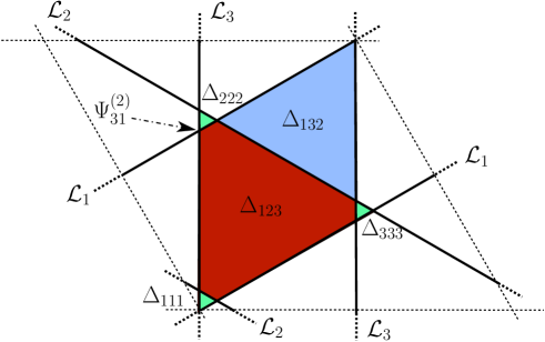
Figure 3: Shown is the fundamental region of the cubic torus at $\rho=e^{2\pi i/3}$, with the three special lagrangian $D$-branes ${\mathcal{L}}_{i}$ on top. The triangular world-sheets $\Delta_{abc}$ shown give the leading instanton corrections to the Yukawa couplings $C_{abc}$. Note that we have slightly shifted ${\mathcal{L}}_{2}$ by setting $u_{2}\not=0$, so that each of the three triple intersections gets resolved into three pairwise intersections, and the $\Delta_{aaa}$ get a non-vanishing area. The boundary changing open string operators $\Psi_{ij}^{(a)}$ are localized at the corresponding intersection points of the branes ${\mathcal{L}}_{j}$ and ${\mathcal{L}}_{i}$ (an example of which is indicated).

Now recall that our parametrization of the jacobian in (21) was such that we had switched on certain Wilson lines and position shifts. Undoing these translations (the choice of origin on the jacobian is of course immaterial), we finally obtain for the 3-point functions:

$$C_{111}(\tau,\xi)\ = \ e^{6\pi i\xi_{1}\xi_{2}}q^{3{\xi_{2}}^{2}/2}\,\sum_{m}q^{3m^{2}/2}e^{6\pi im\xi}$$

$$C_{123}(\tau,\xi)\ = \ e^{6\pi i\xi_{1}\xi_{2}}q^{3{\xi_{2}}^{2}/2}\,\sum_{m}q^{3(m+1/3)^{2}/2}e^{6\pi i(m+1/3)\xi}$$ (40)

$$C_{132}(\tau,\xi)\ = \ e^{6\pi i\xi_{1}\xi_{2}}q^{3{\xi_{2}}^{2}/2}\,\sum_{m}q^{3(m-1/3)^{2}/2}e^{6\pi i(m-1/3)\xi}\ ,$$

where $\xi\equiv\xi_{1}+\tau\xi_{2}=u_{1}+u_{2}+u_{3}$. In $A$-model language where $\tau\rightarrow\rho$, the interpretation [32, 20] of these $\Theta$-functions is that they count the areas of the disk instantons that are bounded by the three intersecting $D$-branes ${\mathcal{L}}_{i}$ ($q=e^{2\pi i\rho}\sim e^{-2\pi\,{\rm Area}}$). This is visualized in Fig. 3. The $\xi$-dependence takes position shifts and Wilson lines on the $A$-branes into account. The expressions (4) coincide with the Yukawa couplings given in [33], which were obtained by a direct evaluation of the areas of the triangles and summing them up.

5 Fukaya products and $\Theta$-identities

One may wonder what the underlying mathematical reason is why the triple matrix product of the $\Psi$’s yields the correct disk partition functions (4). We have already mentioned that the result arises due to non-trival addition formulae of $\Theta$-functions on which the $\Psi$’s depend. On the other hand we know from [20, 21, 22, 23, 24] that certain such formulae represent Fukaya products of the derived category on the elliptic curve. It is thus desirable to exhibit this connection more explicitly, by identifying the kind of $\Theta$-function identities that underly our results.

Specifically, for general vector bundles on the elliptic curve, the first non-zero, associative Fukaya product $m_{2}:\$Hom$[{\mathcal{L}}_{i},{\mathcal{L}}_{j}]\otimes$Hom$[{\mathcal{L}}_{j},{\mathcal{L}}_{k}]\rightarrow$Hom$[{\mathcal{L}}_{i},{\mathcal{L}}_{k}]$ can be written in the following form [20, 21, 22, 23]:

$$m_{2}([e_{ij}(0,a),[e_{jk}(0,b)])\ =\ \sum_{n\in I_{\lambda_{j}}/I_{\lambda_{i}\lambda_{j}\lambda_{k}}}\Theta_{I_{\lambda_{i}\lambda_{j}\lambda_{k}};n}(p\tilde{\rho})\,[e_{ik}(n,-\lambda_{j}n+a+b)]\ ,$$ (41)

where $[e_{ij}(m,k)]$ denote basis elements of Hom$[{\mathcal{L}}_{i},{\mathcal{L}}_{j}]$, and the arguments denote certain lattice shifts further explained in [21, 22, 23]. Moreover, $\lambda=c_{1}/r$ denotes the slopes of the branes, and $I_{\lambda_{i}}=\{n\in{\mathbb{Z}}:n\lambda_{i}\in{\mathbb{Z}}\}$, $I_{\lambda_{i}\lambda_{j}\lambda_{k}}=I_{\lambda_{j}}\cap\frac{\lambda_{k}-\lambda_{i}}{\lambda_{k}-\lambda_{j}}\lambda_{i}$. Furthermore, $p=\frac{(\lambda_{k}-\lambda_{j})(\lambda_{j}-\lambda_{i})}{\lambda_{k}-\lambda_{i}}$ and $\Theta_{I;n}$ denotes a $\Theta$-function of the form (20), but for which the sum runs over $m\in I+n$.

The product (41) takes the form of a $\Theta$-function identity when the basis elements $[e_{ij}]$ are represented by sections made out of $\Theta$-functions. This is particularly simple for line bundles, where $r({\mathcal{L}}_{i})=1$, $\lambda_{i}\in{\mathbb{Z}}$ and for which the $[e_{ij}]$ are directly given by $\Theta$-functions: $[e_{ij}(0,a)]\sim\Theta_{(\lambda_{j}-\lambda_{i}){\mathbb{Z}},a}(\frac{\tilde{\rho}}{\lambda_{j}-\lambda_{i}})$. For more general vector bundles with $r({\mathcal{L}}_{i})>1$ (which applies to our example), one needs to employ isogenies (rescalings of $\tilde{\rho}$), and consider $r$-tuples of sections; see [20, 21, 22, 23, 24] for details.

For the case at hand, we identify the labels as $(i,j,k)=(2,1,3)$, and we have for the slopes $\lambda_{\ell}=\lambda({\mathcal{L}}_{\ell})$ of the bundles: $\lambda_{1}=1/2$, $\lambda_{2}=-1$, $\lambda_{3}=2$ which yields $p=3/4$. Because of $I_{\lambda_{\ell}}=2{\mathbb{Z}}=I_{\lambda_{2}\lambda_{1}\lambda_{3}}$, the sum in (41) runs only over $n=0$. The resulting $\Theta$-function on the RHS of (41), given by $\Theta_{2{\mathbb{Z}},0}(3/4\tilde{\rho})$, precisely coincides with the Yukawa couplings given in the previous section. Moreover, the $[e_{ij}]$ can be represented by sections of Hom$[{\mathcal{L}}_{i},{\mathcal{L}}_{j}]\cong H^{0}(L^{\otimes 3})$, which is three-dimensional and is generated by $\alpha_{\ell}(-u_{j}-u_{i})$.

To make contact with our Landau-Ginzburg computations, notice that the result (4) for the correlators (32) can be expressed by the following operator product:

$$\Psi_{21}^{(a)}(u_{2},u_{1})\cdot\Psi_{13}^{(b)}(u_{1},u_{3})\ =\ \sum C_{ab}^{\ \ c}(\tilde{\rho},u_{1}+u_{2}+u_{3})\,\Phi_{23}^{(c)}(u_{2},u_{3})\ ,$$ (42)

(modulo $Q$-exact pieces). This is nothing but the $B$-model mirror Landau-Ginzburg representation of the Fukaya product (41). The $[e_{ij}]$ are represented here by the matrix-valued, ${\mathbb{Z}}_{3}$ equivariant sections $\Psi_{ji}^{(a)}$ and $\Phi_{ij}^{(a)}$ as given in Section 2, with the proper normalizations. Specifically, recalling that the $\Psi$’s were already rescaled by $c_{ij}$ defined below (36), and implementing the rescaling mentioned at the end of the previous section, it follows that the normalization functions in ${\mathcal{Q}}$ for the fermionic ring elements can be chosen as follows:

$$g^{(b)}_{i+1\,{\rm mod}\,3,i}\ =\ \Big{(}\frac{q(\tilde{\rho})}{\eta(\tilde{\rho})}\Big{)}^{-1/3}\ =\ {\rm const.}({a}^{\prime})^{1/4}(1-{a}^{3})^{-5/24}\ ,\ \ b=1,2,3,$$ (43)

where we have used $\eta^{8}=\frac{3}{(2\pi i)^{2}}\frac{({a}^{\prime})^{2}}{{a}^{3}-1}$. The bosonic normalizations are then fixed by (35), and in particular we find:

$$g^{(1)}_{23}\ =\ {\rm const.}({a}^{\prime})^{1/4}(1-{a}^{3})^{-7/24}\Big{(}\alpha_{2}(u_{2})\alpha_{2}(u_{3})\alpha_{3}(u_{2})\alpha_{3}(u_{3})\alpha_{3}(-u_{2}-u_{3})\Big{)}^{-1}.$$ (44)

Using these normalizations, and by repeatedly using the cubic equation (4), we find that, for example, the product $m_{2}(\Psi^{1}_{21}\Psi^{1}_{13})=\alpha_{1}(u_{1}+u_{2}+u_{3})\Phi^{1}_{23}$ boils down to the following identity between $\Theta$-functions:

$$\frac{1}{\eta(\tilde{\rho})\alpha_{1}(u_{1})}\Bigg{(}\frac{\alpha_{2}(-u_{3}-u_{1})\alpha_{3}(-u_{2}-u_{1})}{\alpha_{2}(u_{2})\alpha_{3}(u_{3})}-\frac{\alpha_{2}(-u_{2}-u_{1})\alpha_{3}(-u_{3}-u_{1})}{\alpha_{2}(u_{3})\alpha_{3}(u_{2})}\Bigg{)}$$ (45)

$$\qquad=\qquad\alpha_{1}(u_{1}+u_{2}+u_{3})\,\frac{\alpha_{1}(u_{3}-u_{2})}{\alpha_{2}(u_{2})\alpha_{2}(u_{3})\alpha_{3}(u_{2})\alpha_{3}(u_{3})}\ ,$$ (46)

whose left- and right-hand sides correspond to eq. (41); the other products lead to analogous expressions, and we do not need to present them here. Noting that the denominator on the RHS stems from the normalization of $\Phi^{1}_{23}$, we see that the structure of the RHS is quite simple; this is a reflection of the fact that the involved bundles ${\mathcal{L}}_{2}\sim{\mathcal{O}}(-1)$, ${\mathcal{L}}_{3}\sim{\mathcal{O}}(2)$ are line bundles, for which the morphisms are simple $\Theta$-functions. On the other hand, the LHS ist structurally more complicated, and this reflects the involvement of ${\mathcal{L}}_{1}$ which is a rank two bundle.

Summarizing, we have demonstrated that the boundary Landau-Ginzburg approach reproduces non-trivial mathematical results about the category of $D$-branes on the elliptic curve. We expect it to capture branes with higher $K$-charges and also the higher products $m_{k}$ (though likely with considerably more effort), as well as generalizations to branes on higher dimensional manifolds; this will be discussed elsewhere.

Acknowledgments We would like to thank Kentaro Hori and Calin Lazaroiu for collaborative input into this project. We are most grateful to Alexander Polishchuk and Daniel Roggenkamp for enlightening discussions. I.B. thanks ETH Zürich for hospitality, and W.L. and J.W. acknowledge the ICMS in Edinburgh and the organizers of the very stimulating Workshop on Derived Categories, Quivers and Strings at which parts of this work were done. This research was supported in part by the National Science Foundation under Grant No. PHY99-07949.

Appendix: LG description of the short diagonals.

The $3\times 3$ matrix factorizations discussed in the main part of the paper do not describe the minimal branes, i.e., the generators of the full $K$-charge lattice on the torus. These have slopes $(r,c_{1})=(1,0)$ and $(0,1)$, corresponding to pure $D2$ and $D0$ branes, and are the $B$-model mirrors of the short diagonals ${\mathcal{S}}_{1}$, ${\mathcal{S}}_{2}$, ${\mathcal{S}}_{3}$ of the $SU(3)$ torus, as shown in Fig. 1. The minimal branes do not arise as pull-backs from the ambient ${\mathbb{P}}^{2}$, but are intrinsically tied to the curve $W=0$ in ${\mathbb{P}}^{2}$.

In this appendix, we study a class of ${\mathbb{Z}}_{3}$-equivariant, quasi-homogeneous $2\times 2$ matrix factorizations of the cubic (1), that describe these minimal branes. At $a=0$, such matrix factorizations were discussed in [25]. Analogous branes for the quintic at the Fermat point have been obtained in [6], where it was shown that they provide an integral basis of the full charge lattice.

We start with the following system of homogeneous linear functions:

$$L_{1} = \alpha_{3}x_{1}-\alpha_{2}x_{3}$$

$$L_{2} = -\alpha_{3}x_{2}+\alpha_{1}x_{3}.$$

For $\alpha_{3}=0$ the linear equations $L_{1}=L_{2}=0$ describe a point which lies on the torus provided that the $\alpha_{i}$ fulfill the torus equation (1). We can then find two polynomials $F_{1},F_{2}$ of degree $2$ such that

$$\alpha_{1}\alpha_{2}\alpha_{3}W=L_{1}F_{1}+L_{2}F_{2}.$$

Explicitly, $F_{1},F_{2}$ can be chosen to be

$$F_{1} = \alpha_{1}\alpha_{2}x_{1}^{2}+\alpha_{2}^{2}x_{1}x_{2}-\alpha_{1}^{2}x_{2}^{2}-\alpha_{1}\alpha_{3}x_{3}^{2}$$

$$F_{2} = \alpha_{2}^{2}x_{1}^{2}-\alpha_{1}^{2}x_{1}x_{2}-\alpha_{1}\alpha_{2}x_{2}^{2}+\alpha_{3}^{2}x_{1}x_{3}.$$

Under the exchange $x_{i}\leftrightarrow\alpha_{i}$ the polynomials transform as $L_{1}\leftrightarrow L_{2}$ and $F_{1}\leftrightarrow-F_{2}$.

Note that the factorization becomes singular in the limit $\alpha_{3}\to 0$, since the equations $L_{1}=L_{2}=0$ fail to describe a point in that case. To cover this coordinate patch, one has to use linear combinations of $L_{1},L_{2}$ that are well-behaved in the limit, such as the system consisting of $\tilde{L}_{1}$ and $\tilde{L}_{2}=\frac{1}{\alpha_{3}}(\alpha_{1}L_{1}+\alpha_{2}L_{2})$ and $\tilde{F}_{1}=F_{1}-\frac{\alpha_{1}}{\alpha_{2}}F_{2}$ and $\tilde{F}_{2}=\frac{\alpha_{3}}{\alpha_{2}}F_{2}$.

The BRST operator takes the form

$$Q=\tilde{L}_{1}\pi_{1}+\tilde{L}_{2}\pi_{2}+\frac{1}{\alpha_{1}\alpha_{2}\alpha_{3}}(\tilde{F}_{1}\bar{\pi}_{1}+\tilde{F}_{2}\bar{\pi}_{2}),$$

where $\pi_{i},\bar{\pi}_{i}$ form a representation of the four dimensional Clifford algebra. It can also be written in the form (2) with $J=\left(\begin{smallmatrix}\tilde{L}_{1}&\tilde{F}_{2}\\ -\tilde{L}_{2}&\tilde{F}_{1}\end{smallmatrix}\right)$ and $E=\frac{1}{\alpha_{1}\alpha_{2}\alpha_{3}}\left(\begin{smallmatrix}\tilde{F}_{1}&-\tilde{F}_{2}\\ \tilde{L}_{2}&\tilde{L}_{1}\end{smallmatrix}\right)$.

To verify that the $2\times 2$ factorizations correspond to the short diagonals in the $A$-picture, we determine their charges. This can easily be done by first determining their intersection numbers with the $3\times 3$-factorization type of branes. In a second step one can then determine a collection of $3\times 3$ branes which have the same intersection numbers with any other set of $3\times 3$ branes as the $2\times 2$ branes. The charge of this collection of $3\times 3$ branes is known from our earlier considerations and equals the charge of the $2\times 2$ branes.

The intersection numbers of the $2\times 2$ factorizations with the $3\times 3$ factorizations have been determined in [6]. In that paper, all computations were done exclusively at the Gepner point, but since the intersection numbers are topological, we can make use of their calculations. The result is that the intersection matrix is

$$I_{2\times 2,3\times 3}=-1+2g-g^{2},$$ (47)

where $g$ is the ${\mathbb{Z}}_{3}$ shift matrix that shifts the ${\mathbb{Z}}_{3}$ representation label of a brane by one. For our calculation, we need in addition the intersection matrix of the $3\times 3$ branes, which is given by

$$I_{3\times 3,3\times 3}=-3g+3g^{2}.$$

We now look for a stack of $x_{i}$ branes of type ${\mathcal{L}}_{i}$ having th intersection numbers (47). This amounts to the following equation:

$$(-3g+3g^{2})(x_{1}+x_{2}g+x_{3}g^{2})=-1+2g-g^{2},$$

with the solution $x_{1}=-\frac{2}{3}+x_{3},x_{2}=-\frac{1}{3}+x_{3}$. Translating this into charges, the first of the three $2\times 2$ branes has the charge of $q_{1}=-1/3(2q({\mathcal{L}}_{3})+q({\mathcal{L}}_{1}))=(0,1)$ and is a pure D0 brane, confirming the expectation that one of the branes should be a pure D0 brane. The charges of the other two branes are $q_{2}=-1/3(2q({\mathcal{L}}_{2})+q({\mathcal{L}}_{3}))=(1,0)$, which is a pure D2 brane, and $q_{3}=-1/3(2q({\mathcal{L}}_{1})+q({\mathcal{L}}_{2}))=(-1,-1)$. To find the interpretation of the branes in the A-type picture, we note that $2$ times a long diagonal plus $1$ times the ${\mathbb{Z}}_{3}$ rotated long diagonal yields $3$ times a short long diagonal, such that the $2\times 2$ factorizations indeed correspond to the branes ${\mathcal{S}}_{i}$ wrapped along the short diagonals (see Figure 1).

We can give another consistency check of our results by determining the flat brane modulus as we did in section 3 for the $3\times 3$ factorizations. In the same notation, and in the same normalization as in eq. (28), we find for the $2\times 2$ factorizations

$$\langle\partial_{u}Q\rangle_{\rm disk,normalized}=\frac{1}{3}f(\tau,u)\,,$$ (48)

where $f$ is as in (29). The $\alpha_{\ell}$, then, have to be identified with $\Theta$-functions as in (21), with $3u\to u$.

References

• [1] K. Hori, S. Katz, A. Klemm, R. Pandharipande, R. Thomas, C. Vafa, R. Vakil, and E. Zaslow, Mirror Symmetry. American Mathematical Society, 2003.
• [2] A. Kapustin and Y. Li, “D-branes in Landau-Ginzburg models and algebraic geometry,” JHEP 12 (2003) 005, hep-th/0210296.
• [3] I. Brunner, M. Herbst, W. Lerche, and B. Scheuner, “Landau-Ginzburg realization of open string TFT,” hep-th/0305133.
• [4] A. Kapustin and Y. Li, “Topological correlators in Landau-Ginzburg models with boundaries,” Adv. Theor. Math. Phys. 7 (2004) 727–749, hep-th/0305136.
• [5] A. Kapustin and Y. Li, “D-branes in topological minimal models: The Landau-Ginzburg approach,” hep-th/0306001.
• [6] S. K. Ashok, E. Dell’Aquila, and D.-E. Diaconescu, “Fractional branes in Landau-Ginzburg models orbifolds,” hep-th/0401135.
• [7] S. K. Ashok, E. Dell’Aquila, D.-E. Diaconescu, and B. Florea, “Obstructed D-branes in Landau-Ginzburg models orbifolds,” hep-th/0404167.
• [8] K. Hori and J. Walcher, “F-term equations near Gepner points,” hep-th/0404196.
• [9] M. Herbst, C.-I. Lazaroiu, and W. Lerche, “D-brane effective action and tachyon condensation in topological minimal models,” hep-th/0405138.
• [10] M. Herbst and C.-I. Lazaroiu, “Localization and traces in open-closed topological Landau-Ginzburg models,” hep-th/0404184.
• [11] A. Kapustin and L. Rozansky, “On the relation between open and closed topological strings,” hep-th/0405232.
• [12] N. P. Warner, “Supersymmetry in boundary integrable models,” Nucl. Phys. B450 (1995) 663–694, hep-th/9506064.
• [13] S. Govindarajan, T. Jayaraman, and T. Sarkar, “Worldsheet approaches to D-branes on supersymmetric cycles,” Nucl. Phys. B580 (2000) 519–547, hep-th/9907131.
• [14] S. Govindarajan and T. Jayaraman, “On the Landau-Ginzburg description of boundary CFTs and special Lagrangian submanifolds,” JHEP 07 (2000) 016, hep-th/0003242.
• [15] S. Govindarajan, T. Jayaraman, and T. Sarkar, “On D-branes from gauged linear sigma models,” Nucl. Phys. B593 (2001) 155–182, hep-th/0007075.
• [16] K. Hori, “Linear models of supersymmetric D-branes,” hep-th/0012179.
• [17] M. Kontsevich. unpublished.
• [18] D. Orlov, “Triangulated categories of singularities and D-branes in Landau-Ginzburg models,” math.ag/0302304.
• [19] M. Herbst, C.-I. Lazaroiu, and W. Lerche, “Superpotentials, ${A}_{\infty}$ relations and WDVV equations for open topological strings,” hep-th/0402110.
• [20] A. Polishchuk and E. Zaslow, “Categorical mirror symmetry: The elliptic curve,” Adv. Theor. Math. Phys. 2 (1998) 443–470, math.ag/9801119.
• [21] A. Polishchuk, “Massey and Fukaya products on elliptic curves,” math.AG/9803017.
• [22] A. Polishchuk, “Homological mirror symmetry with higher products,” math.AG/9901025.
• [23] A. Polishchuk, “${A}_{\infty}$-structures on an elliptic curve,” math.ag/0001048.
• [24] A. Polishchuk, “M. P. Appel’s function and vector bundles of rank 2 on elliptic curves,” math.AG/9810084.
• [25] R. Laza, G. Pfister, and D. Popescu, “Maximal Cohen-Macaulay modules over the cone of an elliptic curve,” J. Algebra 253 (2002) 209.
• [26] I. Brunner, M. R. Douglas, A. E. Lawrence, and C. Romelsberger, “D-branes on the quintic,” JHEP 08 (2000) 015, hep-th/9906200.
• [27] F. Klein and R. Fricke, Vorlesungen über die Theorie der elliptischen Modulfunktionen. B. G. Teubner, 1890.
• [28] W. Lerche, D. Lüst, and N. Warner, “Duality symmetries in N=2 Landau-Ginzburg models,” Phys. Lett. B231 (1989) 417.
• [29] W. Lerche, D. J. Smit, and N. P. Warner, “Differential equations for periods and flat coordinates in two-dimensional topological matter theories,” Nucl. Phys. B372 (1992) 87–112, hep-th/9108013.
• [30] W. Lerche, P. Mayr, and N. Warner, “N = 1 Special Geometry, mixed Hodge variations and toric geometry,” hep-th/0208039.
• [31] D. Mumford, Tata Lectures on Theta, vol. I. Birkhäuser, 1983.
• [32] M. Kontsevich, “Homological algebra of mirror symmetry,” in Proceedings of the International Congress of Mathematicians, Vol. 1, 2 (Zürich, 1994), (Basel), pp. 120–139, Birkhäuser, 1995.
• [33] D. Cremades, L. E. Ibanez, and F. Marchesano, “Yukawa couplings in intersecting D-brane models,” JHEP 07 (2003) 038, hep-th/0302105.