NORDITA-2004-73, UPRF-2004-14

Information on the Super Yang-Mills Spectrum

^a A. Feo , ^b P. Merlatti and ^b F. Sannino

^a Dipartimento di Fisica, Università di Parma and INFN Gruppo

Collegato di Parma, Parco Area delle Scienze, 7/A. 43100 Parma, Italy.

^b NORDITA, Blegdamsvej 17, DK-2100 Copenhagen Ø, Denmark

We investigate the spectrum of the lightest states of $N=1$ Super Yang-Mills. We first study the spectrum using the recently extended Veneziano Yankielowicz theory containing also the glueball states besides the gluinoball ones. Using a simple Kähler term we show that within the effective Lagrangian approach one can accommodate either the possibility in which the glueballs are heavier or lighter than the gluinoball fields.

We then provide an effective Lagrangian independent argument which allows, using information about ordinary QCD, to deduce that the lightest states in super Yang-Mills are the gluinoballs. This helps constraining the Kähler term of the effective Lagrangian. Using this information and the effective Lagrangian we note that there is a small mixing among the gluinoball and glueball states.

1 Introduction

Strongly interacting supersymmetric gauge theories are much studied since, in many respects, they resemble Quantum Chromodynamics. Theoretically we already know a great deal about supersymmetric gauge theories which are closer to their non supersymmetric cousins, namely $N=1$ supersymmetric gauge theories, see [1] for a review. Here we show that it is also possible to use the present experimental knowledge of QCD to learn about super Yang-Mills non perturbative dynamics.

Gaining information on the spectrum of $N=1$ super Yang-Mills is the goal of this paper. We will provide a definite answer to the question of which state is the lightest supersymmetric state in super Yang-Mills. We will compare the $R=2$ sector of the theory whose representative is the gluinoball superfield with the $R=0$ sector, which is a glueball state. We will study the mixing as well.

The tools we will use to make our predictions are: i) The newly extended Veneziano and Yankielowicz (VY) [2] effective Lagrangian which, besides the $R=2$ sector, consistently includes the $R=0$ sector [3]; ii) The relation between QCD with one flavor and super Yang-Mills recently advocated in [4] and further studied in [5]. To make such a correspondence one uses a large $N$ limit in which a Dirac fermion is in the two index antisymmetric representation of the $SU(N)$ gauge theory. This limit was first introduced in [6] and further studied in [7]; iii) The knowledge of the QCD spectrum from experiments and lattice computations.

Our exploration starts with the effective superpotential built in terms of two chiral superfields constituting the minimal set of superfields needed to fully describe the vacuum of super Yang-Mills [2, 3]. The two chiral superfields are respectively the $R=2$ gluinoball chiral superfield and the $R=0$ glueball chiral superfield. To be able to discuss the spectrum we augment the superpotential by a Kähler term. We then proceed to show that within the effective Lagrangian approach one can accommodate either the possibility in which the glueballs are heavier or lighter than the gluinoball fields. This is not too surprising since, even though the superpotential in [3] has no free parameters, the Kähler term is not constrained. However once the mass ordering of the states is determined this effective theory can be used to understand the mixing between these states.

Using the information about ordinary QCD and the large $N$ relation discussed above we predict the gluinoball to be lightest state of super Yang-Mills.

The knowledge of which state is the lightest is then used to constrain the effective Kähler term. This allows us to show that the mixing among the gluinoball and glueball is small.

The paper is organized as follows. In section 2 we study the $N=1$ SYM spectrum via the extended VY effective Lagrangian. In section 3 we provide the Lagrangian free prediction of which is the lightest state of super Yang-Mills while in section 4 we compare our results with existing lattice results. We finally conclude in section 5.

2 Spectrum via Extended VY Lagrangian

Effective Lagrangians are an important tool for describing strongly interacting theories in terms of their relevant degrees of freedom. The well known VY effective Lagrangian constructed in [2] economically describes the vacuum structure of super Yang-Mills. It concisely summarizes the symmetry of the underlying theory in terms of a “minimal” number of degrees of freedom which are encoded in the superfield $S$

$$S=\frac{3}{32\pi^{2}\,N}{\rm Tr}W^{2}\ ,$$ (1)

where $W_{\alpha}$ is the supersymmetric field strength. When interpreting $S$ as an elementary field it describes a gluinoball and its associated fermionic partner. In this paper we follow the notation introduced in [5].

Besides the gluinoballs with non zero $R$-charge also glueball states with zero $R$ charge are important degrees of freedom. These states play a relevant role when breaking supersymmetry by adding a gluino mass term [3]. This is so since the basic degrees of freedom of the pure Yang-Mills theory are glueballs. Further support for the relevance of such glueball states in super Yang-Mills comes from lattice simulations [11]. And finally it has been shown in [3] that these new states are needed to provide a more consistent picture of the vacuum of super Yang Mills via an effective Lagrangian description.

However no physical glueballs appear in the VY effective Lagrangian. In this paper we employ the extended VY Lagrangian, provided in [3], which takes into account the glueball states via the introduction of a chiral superfield $\chi$ with the proper quantum numbers. The constraint used to construct the effective superpotential involving $S$ and $\chi$ has been to reproduce the anomalies of super Yang-Mills while keeping unaltered the vacuum structure. This led to a general form of the superpotential in terms of an undetermined function of the chiral field $f(\chi)$. It has, nevertheless, been possible to motivate a specific form for $f(\chi)$ which has a number of amusing properties. For example the $N$ vacua of the theory emerge naturally when integrating out the glueball superfield $\chi$ as suggested first in [12]. This intriguing relation seems moreover to have a natural counterpart in the geometric approach to the effective Lagrangian theory proposed by Dijkgraaf and Vafa [13]. Another important check is related to supersymmetry breaking. When adding a gluino mass to the theory the same choice of the function $f(\chi)$ leads to a Kähler independent part of the “potential” which has the same functional form of the glueball effective potential for the non supersymmetric Yang-Mills theory developed and used in [14].

In [3] the focus was on the properties of the theory which depends solely on the superpotential which reads:

$$W\left[S,\chi\right] = \frac{2N}{3}S\left[\ln\left(\frac{S}{\Lambda^{3}}\right)^{N}-N-N\ln\left(-e\frac{\chi}{N}\ln\chi^{N}\right)\right]\ ,$$ (2)

where $S$ is the gaugino bilinear superfield ($S=\varphi+\sqrt{2}\theta\psi+\theta^{2}F$) and $\chi$ describes the $R=0$ glueball type degrees of freedom, ($\chi=\varphi_{\chi}+\sqrt{2}\theta\psi_{\chi}+\theta^{2}F_{\chi}$).

A Kähler is needed for computing the spectrum. VY suggested the simplest Kähler for $S$, i.e. $(SS^{{\dagger}})^{1/3}$ which does not upset the saturation of the quantum anomalies. We modify the VY Kähler to provide a kinetic term also for $\chi$ as follows:

$$K(S,S^{{\dagger}},\chi,\chi^{{\dagger}})~{}=~{}\frac{9\,N^{2}}{\alpha}(SS^{{\dagger}})^{1/3}(1~{}+~{}\gamma\,\chi\chi^{{\dagger}})\ ,$$ (3)

where $\gamma$ is a positive number. A more general Kähler can be constructed with an arbitrary function of $\chi$ and $\chi^{{\dagger}}$. We however expect the simplest choice to provide a reasonable description of the mass spectrum.

To compute the potential of the theory we need the Kähler metric which is:

$$g^{l\bar{m}}=\left[g_{l\bar{m}}^{-1}\right]^{T}\ ,\quad{\rm with}\quad g_{l,\bar{m}}=\frac{\partial^{2}\,K}{\partial\varphi^{l}\partial\bar{\varphi}^{\bar{m}}}\ ,$$ (4)

and $\varphi^{1}=\varphi$ while $\varphi^{2}=\varphi_{\chi}$. The potential is then

$$V\left[\varphi\ ,\varphi_{\chi}\right]=\frac{\partial W}{\partial\varphi^{l}}\,g^{l\bar{m}}\,\frac{\partial W^{\dagger}}{\partial\bar{\varphi}^{\bar{m}}}\ .$$ (5)

Given the extended VY Lagrangian and the simple Kähler term we introduced we derive

$$V\left[\varphi\ ,\varphi_{\chi}\right] = \left(\varphi\bar{\varphi}\right)^{\frac{2}{3}}\frac{4N^{2}\,\alpha}{9}\left[\left|\ln\left(\frac{\varphi}{-e\varphi_{\chi}\ln\varphi_{\chi}}\right)\right|^{2}+\frac{\left(1+\gamma\,\varphi_{\chi}\bar{\varphi}_{\chi}\right)}{9\gamma}\,\left|\frac{\ln\varphi_{\chi}+1}{\varphi_{\chi}\,\ln\varphi_{\chi}}\right|^{2}\right.$$ (6)

$$+ \left.\frac{\ln\varphi_{\chi}+1}{3\ln\varphi_{\chi}}\,\ln\left(\frac{\bar{\varphi}}{-e\bar{\varphi}_{\chi}\ln\bar{\varphi}_{\chi}}\right)+\frac{\ln\bar{\varphi}_{\chi}+1}{3\ln\bar{\varphi}_{\chi}}\,\ln\left(\frac{\varphi}{-e\varphi_{\chi}\ln\varphi_{\chi}}\right)\right]\,.$$

The potential is bounded from below and has a well defined global minimum.

We now turn to the spectrum. Since the theory is supersymmetric, it is sufficient to investigate only the bosonic sector. Holomorphicity of the superpotential also guarantees degeneracy of the opposite parity states.

Before providing the mass eigenvalues and eigenstates and to build up our intuition it is very instructive to consider the two following limits.

2.1 Integrating out $\chi$

Eliminating $\chi$ via its equation of motion at the superpotential level:

$$\frac{\partial W\left[S,\chi\right]}{\partial\chi}=0\,,$$ (7)

yields

$$\chi=1/e\ .$$ (8)

Here we are restricting ourself to the first branch of the logarithm in order to determine the spectrum. The effective Lagrangian is the VY one with $\alpha$ replaced by $\alpha/(1+\gamma/e^{2})$. The supersymmetric spectrum for the $S$ superfield is:

$$M_{S}=\frac{2}{3}\frac{\alpha}{1+\gamma/e^{2}}\Lambda\,.$$ (9)

2.2 Integrating out $S$

It is also interesting to construct the effective Lagrangian for $\chi$ after having integrated out $S$. The equation of motion for $S$ reads:

$$\frac{\partial W\left[S,\chi\right]}{\partial S}=0$$ (10)

yielding

$$S=-e\Lambda^{3}\,\chi\,\ln\chi\,\ .$$ (11)

The effective theory for $\chi$ is then

$${\cal L} = \frac{9N^{2}}{\alpha}\Lambda^{2}\int d^{2}\theta d^{2}\bar{\theta}\left[e^{2}\chi\chi^{\dagger}\ln\chi\ln\chi^{\dagger}\right]^{1/3}\left(1+\gamma\chi\chi^{\dagger}\right)$$ (12)

$$+ \frac{2N^{2}}{3}e\Lambda^{3}\int\,d^{2}\theta\,\chi\ln\chi+{\rm c.c.}\,,$$

while the common mass of the components of the chiral superfield $\chi$ is

$$M_{\chi}=\frac{2}{27}\frac{\alpha\,e^{2}}{\gamma}\Lambda\ .$$ (13)

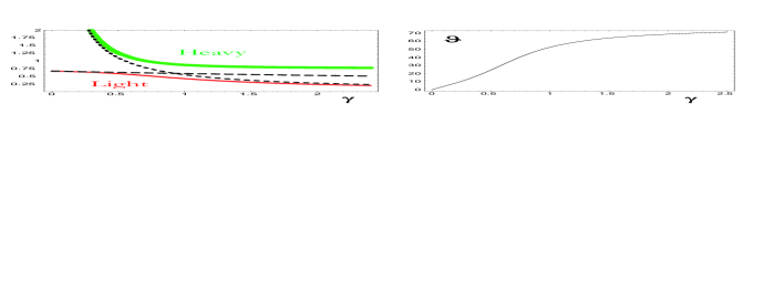
In the left panel of figure 1 we plot the spectrum for the two limiting theories as a function of $\gamma$ after setting $\alpha$ to one. The dashed line represents $M_{S}$ after having integrated $\chi$ out while the dotted line is $M_{\chi}$ after $S$ has been integrated out. Notice that there is a value of $\gamma$ above which the $\chi$ superfield is lighter than the gluinoball field $S$.

2.3 The spectrum and mixing from the effective theory

Diagonalizing the full potential we derived the mass eigenvalues. They are plotted in the left panel of figure 1 as a function of the unknown parameter $\gamma$ while we fixed $\alpha$ to one. The two continuous lines correspond to the physical eigenvalues obtained within our theory. At small $\gamma$ we have the glueball state heavier than the gluinoball state. It is amusing to observe how well the limiting case for $\chi$ approximates the physical spectrum at small and large $\gamma$. Comparing with the glueball spectrum, obtained after having integrated out the $S$ field, we can say that for $\gamma$ large enough there is an inversion and the glueball state is lighter than the gluinoball state. In order to make the statement more precise we define the physical states as:

$$|{\rm Light}\rangle = \cos\vartheta\,|R=2\rangle+\sin\vartheta\,|R=0\rangle\ ,$$

$$|{\rm Heavy}\rangle = -\sin\vartheta\,|R=2\rangle+\cos\vartheta\,|R=0\rangle\ ,$$ (14)

where $|{\rm Light(Heavy)}\rangle$ corresponds to the lightest (heaviest) eigenstate. The state with $R=2$ is the pure gluinoball and the $R=0$ state is the pure glueball type state. The mixing angle as function of $\gamma$ is presented in the right panel of figure 1.

At large $\gamma$ the lower curve corresponds mainly to an $R=0$ state. At small $\gamma$ we have that the lightest state is mainly $R=2$ while the heavy one is an $R=0$ state. We can then say that at small $\gamma$ the gluinoball is the lightest of the two chiral superfields.

Figure 1: Left panel: Physical spectrum as function of $\gamma$. The dashed ($M_{S}$) and the dotted line ($M_{\chi}$) correspond respectively to the case in which $\chi$ or $S$ were integrated out. The two continuous, not straight lines, correspond to the heavy (thick-line) and light (thin-line) physical eigenvalues. At small $\gamma$ we have the glueball state heavier than the gluinoball state. For $\gamma$ large enough there is an inversion and the glueball state is lighter than the gluinoball state. Right Panel: Mixing angle as function of $\gamma$

Although our superpotential has no free parameters the spectrum depends on the Kähler coefficient $\gamma$.

3 Using QCD to determine the lightest super Yang Mills state.

From the previous analysis we learned that the extended VY superpotential [3] while correctly describing the vacuum of SYM alone is not sufficient to disentangle the puzzle of which state is the lightest in super Yang-Mills. We have shown that the poor knowledge of the Kähler term, when two heavy chiral superfield are considered simultaneously, heavily affects the effective Lagrangian ability of making general predictions for the mass ordering of the chiral supermultiplets.

We note, however, that in the literature [15, 16, 17] it has been argued, using an effective Lagrangian constructed via a three form superfield approach, that the glueball states, in the supersymmetric limit are lighter than the gluinoball states. This would correspond to the region of $\gamma>1$ in our case.

The burning question is: Can we construct an argument in favor of a certain general ordering pattern which does not rely on the Kähler’s ambiguities of the effective Lagrangian theory ?

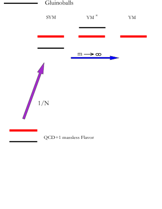
The answer is positive. In fact we can make use of a recent correspondence which, at large $N$, maps the non barionic and bosonic sector of $SU(N)$ Yang Mills theory with one massless Dirac fermion in the two index antisymmetric (symmetric) representation in the bosonic sector of SYM [4]. Interestingly the two index antisymmetric representation for three colors is QCD with one flavor [6]. To be more specific we can map directly the complex gluinoball state into the ordinary $\eta^{\prime}$ particle and the associated scalar partner of one flavor QCD. The super Yang-Mills glueball states are also mapped directly in the ordinary glueball states.

In [5] one was also able to compute the leading $1/N$ corrections and make more quantitative predictions from the use of the large $N$ correspondence for fermions in the two index antisymmetric as well as the two index symmetric representation of the gauge group.

When restricting our attention to the two index antisymmetric theory which interpolates between QCD and super Yang-Mills, till now such a relation has been used to make [4, 5] statements about QCD from the knowledge of super Yang-Mills.

Here we will do the converse, i.e. we use well known properties of QCD to make physical predictions for SYM. Since this is a large $N$ type correspondence we admit, upfront, that our predictions are affected by a 30% error which should however be confronted with the ignorance of the effective Lagrangian’s Kähler term as well as the not definitive lattice results. Notice that the poor knowledge of the Kähler does not reduce the power of the effective Lagrangian for SYM. Having a compact description of gluino and glueball state and the associated vacuum properties is still very relevant. The approach of this subsection complements the effective Lagrangian one while providing new constraints on the Kähler structure.

We start by considering QCD with one massless flavor. Here the low lying composite fields made prevalently of glue are heavier than the low lying mesons while the true lightest states are the $\eta^{\prime}$ and the associated scalar meson.

We can be more precise. We can estimate the one flavor $\eta^{\prime}$ mass by taking the experimental value of the 3 flavor QCD eta prime mass reported on the Particle Data Group (PDG) which is $(957.78\pm 0.14)$ Mev [18] and then use the Veneziano-Witten formula:

$$M^{2}_{\eta^{\prime}}[\rm 1~{}flavor]=\frac{1}{3}M^{2}_{\eta^{\prime}}[\rm 3~{}flavor]\ .$$ (15)

For the scalar partner the experimental situation is more delicate [19]. Although one might be tempted to use the mass of the particle $f_{0}(600)$ quoted in the PDG [18] and investigated in much detail in [20], this state is not a $q\bar{q}$ state [21]. A better candidate for the scalar partner of the $\eta^{\prime}$ is the $f_{0}(1370)$ [18, 20], which is heavier than the $\eta^{\prime}$. This is also consistent with the predictions of [5]. We can average the scalar and pseudoscalar mass for three flavors and then use again the Veneziano-Witten formula, yielding as a common mass:

$$M_{\rm\bar{q}q}[\rm 1~{}flavor]\approx 672.~{}{\rm MeV}\ .$$ (16)

From the lattice formulation of pure Yang-Mills we have that the lightest scalar glueball is in the range of $1730$ Mev [22] and the pseudoscalar glueball is $2590$ Mev [22] yielding as a common averaged mass

$$M_{\rm glueball}\approx 2.16~{}{\rm GeV}\ .$$ (17)

We now neglected the small $N_{f}$ dependence. It is then clear that the glueballs are much heavier than the lightest massive scalar and pseudoscalar $\bar{q}q$ state.

This is even more evident when considering the large N expansion a la ’t Hooft . Here it turns out that the $\eta^{\prime}$ becomes very light at large N while the glueball masses remain large and do not scale to zero. We conclude that the splitting between the low lying mesonic states and the glueball states in one flavor QCD is large in comparison to the invariant scale of the theory:

$$\Delta_{\rm 1-Flavor}=\frac{M_{\rm glueball}-M_{\bar{q}q}}{\Lambda}\approx 5-7\ ,$$ (18)

for a $\Lambda\approx 200-300$ MeV.

We then expect that in super Yang-Mills the splitting between the glueball and the gluinoball is

$$\Delta_{\rm SYM}\sim\Delta_{\rm 1-Flavor}\quad{\rm up~{}to~{}30\%~{}corrections}\ .$$ (19)

This finally suggests that the lightest state in super Yang Mills is the gluinoball. When adding a mass to the gluino we expect that at sufficiently large masses, with respect to the invariant scale of the theory, the gluinoball states becomes heavier than the glueball field. In figure 2 we provide the spectrum as a function of the gluino mass.

Figure 2: Spectrum of the theory as a function of the gluino mass. The thick (thin) line represents the glueball (gluinoball) mass scale. Using the correspondence with QCD (lower end of the diagram) we set the relative ordering of the spectrum in the super Yang Mills case. We then add a gluino. There will, certainly, be a value of the gluino mass of the order of the confining scale above which the gluinoball states is heavier than the glueball state. The corresponding theory is indicated in the figure with YM^∗. For sufficiently large gluino masses the gluino decouples and one is left with the pure YM theory.

The information that the glueball is heavier than the gluinoball implies that the coefficient $\gamma$ appearing in our Kähler is less than one. This means that the mixing between the $R=0$ sector, i.e. the glueballs, and the $R=2$ is small.

4 Spectrum of super Yang-Mills theory from lattice results

In this section we compare our previous expectations with Monte Carlo results for $N=1$ super Yang-Mills theory with dynamical light gluinos, [23, 24, 25, 26, 27], where the bound state mass spectrum is investigated. The formulation of Curci and Veneziano [28] which uses Wilson-type fermions has been used here .

In the numerical simulations with light gluinos a gluino bare mass is introduced which breaks supersymmetry softly. In the Curci and Veneziano formulation the supersymmetric limit coincides with the chiral limit and by studying, for example, the pattern of chiral symmetry breaking, through the study of the first order phase transition of the gluino condensate it is then possible to determine the value of the critical hopping parameter which corresponds to the supersymmetric (chiral) limit (i.e. zero gluino mass). It is also possible to determine the gluino massless limit from the study of the supersymmetric Ward-Takahashi identities.

The restoration of supersymmetry can be checked through the study of the supersymmetry multiplets. Lattice simulations, [23, 24, 25, 26, 27], have been performed for four scalar degrees of freedom and two Majorana fermions. They show a non-trivial mass spectrum of the SYM theory with an $SU(2)$ gauge group. More in detail, [25], the lightest bound state with almost the same mass are the glueball $O^{+}$ and the pseudoscalar component of the gluinoball field, while the heavier supermultiplet contains the pseudoscalar glueball state $O^{-}$ and the scalar gluinoball, also degenerate in mass. The mass difference between states of opposite parity is bigger than the gluino mass used for the simulations [24]. This implies that it does not seems to be an effect of softly broken supersymmetry, as has been also stressed in [17].

Recently, [27], results for larger lattices near the supersymmetric point are presented. The analysis of the spectrum in [27] shows, interestingly, that the pseudo scalar gluinoball is lighter than the other two particles of the lightest supermultiplet at the value of the gluino mass measured. The latter findings seem to be more consistent with our results. These also give further evidence that the older lattice simulations were describing an intermediate regime in which supersymmetry is still badly broken.

5 Conclusions

We have investigated the spectrum of the lightest states of $N=1$ super Yang-Mills. The spectrum was first studied using the recently extended Veneziano Yankielowicz theory containing also the glueball states besides the gluinoball ones. We have shown that by adopting a simple Kähler term the effective Lagrangian approach can accommodate either the possibility in which the glueballs are heavier or lighter than the gluinoball fields. To resolve the ambiguity we have provided an effective Lagrangian independent argument. We used the information about ordinary (one-flavor) QCD and the recent map into the bosonic sector of SYM [4] to deduce that the lightest states in super Yang-Mills are, indeed, the gluinoballs. This observation helps constraining the Kähler term of the effective Lagrangian. Using this information and the effective Lagrangian we have then shown that there is a small mixing among the gluinoball and glueball states.

Finally we conclude that the lightest state is the gluinoball field and it has a small mixing with the glueball state. This supports the use of the VY effective theory with the inclusion of the glueball state [3] needed to provide a more consistent description of the non perturbative aspects of the super Yang-Mills vacuum. Due to the small mixing between the glueball and the gluinoball it is reasonable to compute the super Yang-Mills spectrum via the effective Lagrangians at zero and non zero gluino masses [30] or for the orientifold theories at finite $N$ [5]. Our results also indicate that previous lattice simulations were still far from the supersymmetric limit.

Acknowledgments

We thank P.H. Damgaard, L. Del Debbio, P. Di Vecchia, B. Lucini, P. de Forcrand, R. Narayanan, M. Shifman and M. Teper for useful discussions.

References

- [1] K. A. Intriligator and N. Seiberg, “Lectures on supersymmetric gauge theories and electric-magnetic duality,” Nucl. Phys. Proc. Suppl. 45BC, 1 (1996) [arXiv:hep-th/9509066].
- [2] G. Veneziano and S. Yankielowicz, Phys. Lett. B 113, 231 (1982).
- [3] P. Merlatti and F. Sannino, arXiv:hep-th/0404251. To appear in Physics Review D.
- [4] A. Armoni, M. Shifman and G. Veneziano, Nucl. Phys. B 667 (2003) 170 [arXiv:hep-th/0302163]; A. Armoni, M. Shifman and G. Veneziano, Phys. Rev. Lett. 91 (2003) 191601 [arXiv:hep-th/0307097]; A. Armoni, M. Shifman and G. Veneziano, Phys. Lett. B 579 (2004) 384 [arXiv:hep-th/0309013].
- [5] F. Sannino and M. Shifman, Phys. Rev. D 69, 125004 (2004) [arXiv:hep-th/0309252].
- [6] E. Corrigan and P. Ramond, Phys. Lett. B 87, 73 (1979).
- [7] E. B. Kiritsis and J. Papavassiliou, Phys. Rev. D 42, 4238 (1990).
- [8] P. Di Vecchia, A. Liccardo, R. Marotta and F. Pezzella, arXiv:hep-th/0407038.
- [9] F. Sannino and K. Tuominen, arXiv:hep-ph/0405209.
- [10] D. K. Hong, S. D. H. Hsu and F. Sannino, Phys. Lett. B 597, 89 (2004) [arXiv:hep-ph/0406200].
- [11] I. Montvay, Nucl. Phys. Proc. Suppl. 63, 108 (1998) [hep-lat/9709080]; A. Donini, M. Guagnelli, P. Hernandez and A. Vladikas, Nucl. Phys. B 523, 529 (1998) [hep-lat/9710065]; For a recent review see A. Feo, Nucl. Phys. Proc. Suppl. 119, 198 (2003) [arXiv:hep-lat/0210015].
- [12] A. Kovner and M. A. Shifman, Phys. Rev. D 56, 2396 (1997) [arXiv:hep-th/9702174].
- [13] R. Dijkgraaf and C. Vafa, arXiv:hep-th/0208048.
- [14] J. Schechter, Phys. Rev. D 21 (1980) 3393; C. Rosenzweig, J. Schechter and G. Trahern, Phys. Rev. D21, 3388 (1980); P. Di Vecchia and G. Veneziano, Nucl. Phys. B171, 253 (1980); E. Witten, Ann. of Phys. 128, 363 (1980); P. Nath and A. Arnowitt, Phys. Rev. D23, 473 (1981); A. Aurilia, Y. Takahashi and D. Townsend, Phys. Lett. 95B, 65 (1980); K. Kawarabayashi and N. Ohta, Nucl. Phys. B175, 477 (1980); A. A. Migdal and M. A. Shifman, Phys. Lett. B 114, 445 (1982); J. M. Cornwall and A. Soni, Phys. Rev. D 29, 1424 (1984); Phys. Rev. D 32, 764 (1985); A. Salomone, J. Schechter and T. Tudron, Phys. Rev. D23, 1143 (1981); J. Ellis and J. Lanik, Phys. Lett. 150B, 289 (1985); H. Gomm and J. Schechter, Phys. Lett. 158B, 449 (1985); F. Sannino and J. Schechter, Phys. Rev. D 60, 056004 (1999) [hep-ph/9903359].
- [15] G. R. Farrar, G. Gabadadze and M. Schwetz, Phys. Rev. D 58, 015009 (1998) [arXiv:hep-th/9711166].
- [16] G. R. Farrar, G. Gabadadze and M. Schwetz, Phys. Rev. D 60, 035002 (1999) [hep-th/9806204].
- [17] D. G. Cerdeno, A. Knauf and J. Louis, hep-th/0307198.
- [18] S. Eidelman et al. (Particle Data Group), Phys. Lett. B 592, 1 (2004).
- [19] D. Black, A. H. Fariborz, F. Sannino and J. Schechter, Phys. Rev. D 59, 074026 (1999) [arXiv:hep-ph/9808415].
- [20] F. Sannino and J. Schechter, Phys. Rev. D 52, 96 (1995) [arXiv:hep-ph/9501417]; M. Harada, F. Sannino and J. Schechter, Phys. Rev. D 54, 1991 (1996) [arXiv:hep-ph/9511335]; M. Harada, F. Sannino and J. Schechter, Phys. Rev. Lett. 78, 1603 (1997) [arXiv:hep-ph/9609428]; D. Black, A. H. Fariborz, F. Sannino and J. Schechter, Phys. Rev. D 58, 054012 (1998) [arXiv:hep-ph/9804273].
- [21] M. Harada, F. Sannino and J. Schechter, Phys. Rev. D 69, 034005 (2004) [arXiv:hep-ph/0309206].
- [22] C. J. Morningstar and M. J. Peardon, Phys. Rev. D 60, 034509 (1999) [arXiv:hep-lat/9901004].
- [23] I. Campos et al. [DESY-Münster Collaboration], Eur. Phys. J. C 11, 507 (1999) [arXiv:hep-lat/9903014].
- [24] F. Farchioni et al. [DESY-Münster-Roma Collaboration], Eur. Phys. J. C 23, 719 (2002) [arXiv:hep-lat/0111008].
- [25] I. Montvay, Int. J. Mod. Phys. A 17, 2377 (2002) [arXiv:hep-lat/0112007].
- [26] R. Peetz, F. Farchioni, C. Gebert and G. Münster, Nucl. Phys. Proc. Suppl. 119, 912 (2003) [arXiv:hep-lat/0209065].
- [27] F. Farchioni and R. Peetz, arXiv:hep-th/0407036.
- [28] G. Curci and G. Veneziano, Nucl. Phys. B 292, 555 (1987).
- [29] G. Fleming, J. Kogut, P. Vranas, Phys. Rev. D64 (2001) 034510 [arXiv:hep-lat/0008009].
- [30] A. Masiero and G. Veneziano, Nucl. Phys. B249, 593 (1985).