ITP-UU-04/18
SPIN-04/11
hep-th/0408183

CONFINEMENT AT LARGE $N_{c}$

Abstract
A discussion is given of the confinement mechanism in terms of the Abelian projection scheme, for a general number $N_{c}$ of colors. There is a difficulty in the $N_{c}\rightarrow\infty$ limit that requires a careful treatment, as the charges of the condensing magnetic monopoles tend to infinity. We suggest that Bose condensation of electric or magnetic charges is indicative for the kind of confinement that takes place, but the actual mechanism of confinement depends on other features as well.

1 Introduction: The $\beta$ function.

In the absence of mass terms, field theories used in particle physics often appear to be scale-independent. As is well-known, however, quantization and renormalization of these theories require a scale-dependent cut-off, and the scale dependence in general does not go away in the limit where one sends the cut-off to infinity.[1] If $\mu$ is the average value of the momenta in an amplitude that is computed perturbatively, and if the subtractions are carried out such that the higher-order corrections for this amplitude are kept as small as possible (in order to obtain a reasonably convergent perturbation expansion), then one finds the coupling parameters $g$ to be $\mu$-dependent. In case of QED, one finds the electric charge parameter $e$ to obey[2]

$${\mu\,{\rm d}\over{\rm d}\mu}e^{2}(\mu)=\beta(e^{2})\ ,\qquad\beta(e^{2})={e^{4}\over 6\pi^{2}}N_{f}\ +\ {\cal O}(e^{6})\ .$$ (1.1)

The dominant contribution to $\beta(e^{2})$ comes from the one-loop diagram in the photon propagator, see Fig. 1. It is proportional to the number $N_{f}$ of charged fermion species. If charged scalar fields are present they also contribute to $\beta$, with the same sign.

Figure 1: Dominant contribution to the $\beta$ function for QED and for Yang-Mills.

Before 1970, it was generally believed that all $\beta$ functions in quantum field theories had to be positive. In the Yang-Mills case, however, different results were found[3][4]. The contribution of fermions to $\beta$ is as in the QED case (see Fig. 1, diagram ($b$). The contribution of the gauge bosons themselves, however, is of the opposite sign (Fig. 1, diagram ($c$)). When doing the calculation, in a convenient choice of gauge, one finds a primary term that is like the contribution of scalar particles, with relative strength $+{\textstyle{1\over 6}}$, but in addition a much larger contribution, of relative strength $-1$, from those terms that generate the magnetic moments of the gauge bosons. These are large, since they have spin one and giromagnetic ratio 2. Finally, there is a small negative contribution from the ghosts, diagram ($d$), of strength $-{\textstyle{1\over 12}}$. The net result is

$$\beta(g^{2})={g^{4}\over 12\pi^{2}}(N_{f}-11)+{\cal O}(g^{6})\ ,\quad\mathrm{for}\ SU(2)\ ;$$ (1.2)

$$\beta(g^{2})={g^{4}\over 6\pi^{2}}(2N_{f}-11N_{c})+{\cal O}(g^{6}N_{c}^{2})\ ,\quad\mathrm{for}\ SU(N_{c})\ ,\quad N_{c}>2\ .$$ (1.3)

The $SU(2)$ case deviates only because, there, the usual definition of the color coupling $g$ is chosen with a factor ${\textstyle{1\over 2}}$.

Ignoring the higher order terms, the solution of these equations for the running coupling parameter is

$$g^{2}(\mu)=-{1\over\beta_{2}\,\ln(\mu/\Lambda)}\ ,$$ (1.4)

where $\beta_{2}$ is the coefficient in front of the $g^{4}$ term in the expansion for $\beta$, and $\Lambda$ the fundamental scale parameter of the theory. If $\beta_{2}$ is negative, $\Lambda$ has to be taken small, and perturbation expansion only makes sense at $\mu\gg\Lambda$. Then $g$ tends to zero at large $\mu$, but it explodes as $\mu\downarrow\Lambda$.

Does this behavior of the running coupling parameter for Yang-Mills theories such as QCD imply a permanently confining force between quarks? Today, this is indeed believed to be a quite natural consequence, but in the 1970’s, the problem of completeness was brought up. What does the spectrum of physical states look like? if we exclude free quarks and free gluons, can we then ever establish unitarity of the scattering matrix? The only way to understand how unitarity can be restored, is to view confinement as a new phase of matter. It is related to topological features of the gauge theory.

2 Magnetic and electric confinement

2.1 Magnetic confinement

The first sign of an absolutely confining force emerging in a conventional quantum field theory, came from the study of the Abelian Higgs theory[5]. Take the Lagrangian

$${\cal L}(A,\varphi)={\textstyle{1\over 4}}F_{\mu\nu}F_{\mu\nu}-D_{\mu}\varphi^{\dagger}D_{\mu}\varphi-V(\varphi)\ ,$$ (2.1)

where $\varphi$ is a single, complex scalar field, and $V(\varphi)$ a quartic potential invariant under complex rotations of $\varphi$:

$$V(\varphi)={\textstyle{1\over 2}}\lambda(\varphi^{\dagger}\varphi-F^{2})^{2}\ .$$ (2.2)

Here, $F$ is a fixed parameter. The physical vacuum is described by $\varphi$ staying close to its equilibrium value: $\varphi=Fe^{i\theta}$, where $\theta$ may be arbitrary. $\theta$ is fundamentally unobservable since it is completely gauge-dependent.

If, however, in a ‘sheet’, that is, two-dimensional subspace of space or space-time, $\theta$ rotates over a full $360^{\circ}$, then the $\varphi$ field develops a ‘frustration’: $\varphi$ must be differentiable, because of the derivative terms in ${\cal L}$, and therefore there must be a zero somewhere in the sheet. Moving the sheet along in space, we find that this zero forms a one dimensional line in 3-space, i.e., a vortex. In the immediate vicinity of this vortex, $\varphi$ deviates considerably from its equilibrium value, so that the vortex will carry energy. Away from the vortex, the equilibrium value $F$ (or a rotation thereof) is quickly resumed, and so, the vortex maintains a finite transverse extension. It is a non-trivial, locally stable field configuration.

Some elementary calculations show that this vortex carries magnetic flux. Therefore, if we take a magnetic monopole and its antiparticle, i.e., a north and a south pole, then they will be connected by a vortex, causing an absolutely confining force between them, since the energy is proportional to the vortex’ length.

This phenomenon by itself is not new; it was known to describe the Meissner effect in super-conducting materials. Now we see that it leads to the existence of magnetic vortex lines in the vacuum of the Higgs theory. The magnetic confinement model of this section would only explain confinement of quarks if quarks carried a magnetic monopole charge. It was once thought that quarks indeed carry magnetic monopole charges.

2.2 Electric confinement

This, however, is not the case in QCD; quarks only carry a color-electric monopole charge. Thus, what is needed to understand confinement of quarks is the description of color-electric vortex lines. These are related to the magnetic vortex lines by a dual transformation[6]: $\vec{E}\rightarrow\vec{B}$, $\vec{B}\rightarrow-\vec{E}$. This leaves the homogeneous parts of the Maxwell equations invariant, but replaces electric charges with magnetic ones and vice-versa. Since magnetic monopole charges do tend to occur in non-Abelian gauge theories, one may suspect the occurrence of magnetic super-conductivity: the magnetic monopoles condense.

On the other hand, we must keep in mind that stable magnetic monopoles only seem to occur in theories where a compact gauge group is spontaneously broken into a surviving $U(1)$ subgroup. How can we follow the activities of ‘monopoles’ if the symmetry is not spontaneously broken, as in QCD?

3 The Abelian projection for general $N_{c}$

Apart from the commutator terms in the Lagrangian, there is another fundamental difference between Abelian and non-Abelian gauge theories. In Abelian theories, it is impossible to fix the gauge locally, at some space-time point $x$, without referring to the field configurations at other space-time points, far away from $x$, unless one uses charged scalar fields that must have been added to the system. In a non-Abelian gauge theory, one can fix the non-Abelian part of the gauge redundancy by referring exclusively to the vector potential and at most its first derivatives, at the point $x$ alone. This means that, without adding non-local elements to the Lagrangian, one can rewrite a non-Abelian gauge theory as if it were an Abelian one. The only price one pays is that the new, Abelian, Lagrangian becomes a non-polynomial one. The new gauge group is the Cartan sub-group of the original non-Abelian gauge group.

We call this procedure the Abelian projection[7]. In what follows, we describe it for $SU(N)$ for general $N$. The Cartan sub-group of $SU(N)$ is

$${(U(1))^{N}\over U(1)}\ =\ U(1)^{N-1}\ \subset\ SU(N)\ .$$ (3.1)

Take any component of the (non-Abelian) field tensor, say ${G_{12}}^{i}_{\,j}$. Here, $i$ and $j$ are gauge indices running from 1 to $N$. By selecting out the 12 - direction in Minkowski space, our gauge choice will violate Lorentz invariance. It is not really necessary to break Lorentz invariance; one could have chosen any Lorentz-invariant hermitean matrix constructed from the $G_{\mu\nu}$, but this would be technically more complicated, and no harm is done with our simpler choice.

An Abelian projection is realized by choosing the gauge in which $G_{12}$ is diagonalized:

$$G_{12}(x)=\pmatrix{\lambda_{1}(x)&0&\cdots&0\cr 0&\lambda_{2}(x)&\cdots&0\cr\vdots&\vdots&\ddots&\vdots\cr 0&0&\cdots&\lambda_{N}(x)}\ ,\quad\lambda_{1}\leq\lambda_{2}\leq\cdots\leq\lambda_{N}\ .$$ (3.2)

Indeed, we made use of the $SU(N)$ subgroup of the pure permutations to order the eigenvalues $\lambda_{i}(x)$.

Note that, even if the Jacobian associated with the transformation from the vector fields $A_{\mu}(x)$ to the fields $\lambda_{i}(x)$ may be non-trivial, there are no ghosts associated with it. This is because the transformation is a local one: the Faddeev-Popov field does not have a kinetic term. In this gauge, all off-diagonal field components are physically significant — they are invariant under the remaining (Abelian) $U(1)^{N-1}$ - gauge transformations. Therefore, there are no massless, charged vector bosons. The diagonal components of the photon fields do survive as $N-1$ different species of neutral, massless photons.

The fields which in the original Lagrangian came in the fundamental representation, now split up into $N$ different fields. Their charges with respect to the $N$ subgroups $U(1)$ can be labelled as

$$\vec{Q}=(0,\,\cdots,\,0,\,q,\,0,\,\cdots,\,0)\ .$$ (3.3)

This formula must be understood as describing the coupling to $N$ photons, which themselves are mixed in such a way that the diagonal, ‘baryonic’ $U(1)$ photon is removed from the spectrum of photons, so that $N-1$ independent photon states survive. The quark field component $\psi_{i}(x)$ is coupled, with charge $q$, to the $i^{\mathrm{th}}$ photon.

The charged gluon fields do (partly) survive. Their charge table is

$$\vec{Q}=(0,\,\cdots,0,\,q,\,0,\,\cdots,\,0,\,-q,\,0,,\,\cdots,\,0)\ .$$ (3.4)

Note that they will not couple to the baryonic $U(1)$ - photon.

One would conclude that the emerging scheme is exactly as if we had $N-1$ ordinary Maxwell fields, coupled to particles with various combinations of (Abelian) charges. There is, however, one novelty: the Abelian projection is singular whenever two eigenvalues $\lambda_{i}(x)$ at a given point $x$ coincide. Since the $\lambda_{i}$ were ordered, only two consecutive ones can coincide. In the immediate neighborhood of such a point, the original field $G_{12}(x)$ takes the form

$$G_{12}(x)\simeq\pmatrix{*&|&0&|&*\cr\hline\cr\cr 0&\bigg{|}&\matrix{\lambda_{0}+a_{3}&a_{1}-ia_{2}\cr a_{1}+ia_{2}&\lambda_{0}-a_{3}}&\bigg{|}&0\cr\hline\cr\cr*&|&0&|&*}\ .$$ (3.5)

the two consecutive $\lambda$’s only coincide if $a_{1},\ a_{2},$ and $a_{3}$ all vanish. these three conditions define isolated points in three-space. Indeed, these points have the same characteristics as a magnetic monopole in a Higgs theory with Higgs in the adjoint representation of one of the subgroups $SU(2)$ of $SU(N)$. Thus, at such points we find magnetic monopoles. Aparently, this is the way the non-Abelian $SU(N)$ theory differs fundamentally from just any Abelian $U(1)^{N-1}$ theory: besides the electric charges of the form (3.3) and (3.4), we have magnetic monopoles. With respect to the subgroup $SU(2)$ mentioned above, the monopole charge is in the Abelian subgroup $U(1)$ of $SU(2)$. This means that the magnetic charge table for the monopole is

$$\vec{g}_{m}=(0,\,\cdots,\,0,\,g_{m},\,-g_{m},\,0,\cdots,\,0)\ ;\qquad g_{m}=2\pi/q$$ (3.6)

(the subscript $m$ referring to ‘magnetic’). Note that the quarks obey the minimal Dirac condition

$$\sum_{i=1}^{N}q_{i}g_{mi}=2\pi n\ ,$$ (3.7)

with $n=1$ or 0, while the charged gluon whose charges are in the same $SU(2)$ subgroup has $n=\pm 2$. We see from the table (3.6), that there are $N-1$ monopole types.

“Confinement” now occurs in the following way. The $k^{\mathrm{th}}$ monopole field condenses to cause confinement with respect to the Abelian subgroup $U(1)_{k}\otimes[U(1)_{k+1}]^{-1}$ of $SU(N)$. This means that a vortex emerges that confines charges in $U(1)_{k}$ or anti-charges in $U(1)_{k+1}$, by binding them to anti-charges in $U(1)_{k}$ or charges in $U(1)_{k+1}$. thus, the $k^{\mathrm{th}}$ monopole allows ‘hadrons’ of the type $q_{i}\,\overline{q}_{i}$ but also ‘hadrons of the type $q_{k}\,q_{k+1}$. in other words, either all $U(1)$ charges are neutralized, or the $k^{\mathrm{th}}$ charge must be equal to the $(k+1)^{\mathrm{th}}$ charge.

The latter might seem to be an odd type of hadron, but we have to realize that the $k^{\mathrm{th}}$ monopole does not care about the charges in other channels, and consequently, the collective action of all $N-1$ monopole fields allow only $q_{i}\,\overline{q}_{i}$ objects, or objects where all charges are equal: $\vec{Q}=(q,\,\cdots,\,q)$ to survive as unconfined particles. The latter are the baryons.

We see that, unlike what one would expect, $q_{1}\,\overline{q}_{1}$ is not confined, whereas what one would expect is that only $\sum_{i=1}^{N}q_{i}\,\overline{q}_{i}$ would survive. This, however, is a special feature of our gauge choice: the individual fields $q_{i}\,\overline{q}_{i}$ are indeed gauge-invariant here; we claim that the Abelian projection does yield an accurate description of the spectrum of mesonic states, even if it does not look very realistic; the different states $q_{1}\overline{q}_{1},\ q_{2}\overline{q}_{2}$, etc., are probably strongly mixed.

4 Confinement and Bose condensation of charges

In the $N\rightarrow\infty$ limit, one wishes to rescale the coupling strengths:

$$q={\tilde{q}\over\sqrt{N}}\ ;\qquad g_{m}=\sqrt{N}\,\tilde{g}_{m}\ ;\qquad\tilde{q}\,\tilde{g}_{m}=2\pi\ .$$ (4.1)

This is certainly also what is suggested by the $\beta$ function Eq. (1.3). Consequently, the monopole charge $g_{m}$ itself tends to infinity. This makes the arguments discussed above suspect; the methods of Quantum Field Theories cannot be used to describe the Bose condensation of very strongly interacting fields. Nevertheless, the $\beta$ function of Eq. (1.3) makes one believe that confinement continues to take place as $N\rightarrow\infty$. Indeed, the planar diagrams in this limit remind us of string diagrams, which have confinement built in.

4.1 Intermezzo. Confinement as a universal laws in the non-Abelian sector

In view of the above, one may formulate a conjecture that should hold for all non-Abelian gauge theories:

For all gauge groups except $U(1)$, all physical states are color singlets.

Thus, we claim that magnetic monopoles are not needed to achieve confinement, though they do provide for a very useful signal: their vacuum expectation value. To illustrate the point, let us give an unusual, but totally correct description of the physical particles in the $SU(2)$ sector of the Standard Model.

The fermion doublet, $\psi_{L}$, the quark fields $q_{L}$, the gauge vector potential $A_{\mu}$, and the Higgs field $\varphi_{H}$ are usually described as

$$\psi_{L}=\pmatrix{\nu_{e,L}\cr e_{L}}\ ;\qquad q_{L}=\pmatrix{u_{L}\cr d_{L}}\ ;\qquad A_{\mu}=\pmatrix{W_{\mu}^{+}\cr Z_{\mu}^{0}\cr W_{\mu}^{-}}\ ;$$

$$\varphi_{H}=\pmatrix{F\cr 0}+\tilde{\varphi}\ .$$ (4.2)

However, we can describe all of the physical fields as singlets. The fields $\psi_{L}$, $q_{L}$, $\varphi$ and $A_{\mu}$ are handled as $SU(2)$-quarks and gluons. Apart from renormalization factors and tiny higher order corrections, the $SU(2)$-mesons are

$$\nu_{e,L}=(\varphi_{H}^{*}\cdot\psi_{L})\ ,\qquad u_{L}=(\varphi_{H}^{*}\cdot q_{L})\ ,\qquad Z^{0}_{\mu}=(\varphi_{H}^{*}\cdot D_{\mu}\varphi_{H})\ ,$$ (4.3)

(the latter being “$P$ bound states”). The $SU(2)$-baryons are

$$e_{L}=\varepsilon_{ij}\,\varphi_{H}^{i}\,\psi^{j}_{L}\ ,\qquad d_{L}=\varepsilon_{ij}\,\varphi_{H}^{i}\,q_{L}^{j}\ ;\qquad W^{-}_{\mu}=\varepsilon_{ij}\,\varphi_{H}^{i}\,D_{\mu}\varphi_{H}^{j}\ ,$$ (4.4)

and anti-baryons are constructed similarly. The only difference with QCD is that, here, one can use conventional perturbation expansion to calculate the properties of these particles in the usual way, using the vacuum form (4.2) for the Higgs field.

Thus, we see that, using a somewhat unconventional language, the Standard Model can be dealt with in such a way that both the $SU(3)$ and the $SU(2)$ gauge groups are absolutely confining, the only difference being that the $SU(2)$ gauge force has a scalar field in the elementary representation, and a choice of gauge where this field is aligned in a fixed direction is a good point to do perturbation expansion.

It is in other Higgs theories where the difference between the ‘Higgs mode’ and the ‘confinement mode’ is more profound. If the Higgs were in the adjoint representation, such as in the old Georgi-Glashow model[8] where $SU(2)$ (without $U(1)$) is spontaneously broken into a $U(1)$ subgroup by a Higgs triplet field, then it is not possible to rewrite the electron or the neutrino, which are in the elementary representation, as bound states of fermions and scalars. Nevertheless, electrons and neutrinos are physical particles in this theory; they are ‘exotic hadrons’, and it is more difficult to regard them as gauge-invariant objects.

4.2 Aggregation modes

Thus, the real question in QCD was: why can quarks not emerge as physical particles in the same manner as electrons and neutrons do in the Georgi-Glashow model? The answer to this question is now known: gauge theories such as QCD and the Georgi-Glashow model condense in different aggregation modes; a system can be forced to make a transition from one state into another, but such a transition would necessarily be associated with a phase transition. It is either the electric charges, or the magnetic charges that can undergo Bose condensation as described in the above chapters, but never both.

But, to what extent do we need the existence of electric or magnetic charges to realize either one aggregation state or the other? Could it be that the condensation of the magnetic charges in QCD is to be seen as a consequence rather than the cause of the confinement mechanism?

The close relation between confinement mechanisms and the condensation of charges appears to be indisputable. For instance, it was derived that confinement may occur in an Abelian gauge theory on the lattice. Indeed, this theory also possesses magnetic monopoles, that appear to condense. In our alternative treatment of the Standard model, Subsection 4.1, and notably in the Georgi-Glashow model[8], the Higgs field is taken to have a large vacuum value, meaning that these particles Bose condense. Indeed, also, our treatment of confinement in Section 3 shows that the topological argument works for all $N_{c}$. However, for large $N_{c}$, the relevant coupling parameter is $\tilde{g}^{2}=g^{2}N_{c}$, which means that the electric charges have the strength $\tilde{g}/\sqrt{N_{c}}$, and magnetic charges are combinations of $g_{i}$, with strength $g_{m}=2\pi\sqrt{N_{c}}/\tilde{g}$. Since the interactions among these monopoles clearly tend to infinity at large $N_{c}$, treating them using perturbation expansions in terms of fields becomes questionable.

4.3 Dynamics

Therefore, one may argue that, yes, magnetic monopoles do condense in the confinement mode, even at large values of $N_{c}$, but, no, the actual mechanism of confinement could depend on additional dynamical forces. One expects the hadronic mass scale at large $N_{c}$ to be controlled by its $\Lambda$ parameter (the integration constant in the solutions to the Gell-Mann-Low equation (1.1), (1.3) for the coupling strength), and this depends on $\tilde{g}$, not directly on $g$.

Note that the same arguments could be brought forward concerning the contributions of instantons . Their action, too, depends on $g$ and not $\tilde{g}$, so that one might expect that they are exponentially suppressed at high $N_{c}$. This is actually known not to be the case(See for instance Th. Schaefer’s contribution at this Meeting). We do have a running coupling strength $\tilde{g}$, so that instantons with large sizes are not exponentially suppressed. Similarly then, one might attribute confinement at large $N_{c}$ to large magnetic monopoles.

Large magnetic monopoles would require a fundamentally non-local effective field theory. The question then remains whether it is possible to re-establish locality (to some extent) in an effective local field theory for confinement. A model for that is outlined in the next section.

5 A classically confining theory

Absolutely confining forces can indeed be described totally classically. We now describe such a classical model, also described in Ref.[9]. It will not be renormalizable, and this means that, eventually, one wants to attribute the non-renormalizable terms in the action to quantum effects, so that at small distances, renormalizability is restored.

Our model contains an Abelian Maxwell field $A_{\mu}$, and a neutral, scalar field $\varphi$ that affects the dielectric constant of the vacuum (in a Lorentz-invariant way):

$${\cal L}(A,\varphi)=-{\textstyle{1\over 4}}Z(\varphi)F_{\mu\nu}F_{\mu\nu}-V(\varphi)+J_{\mu}(x)A_{\mu}\ ,$$ (5.1)

where the functions $Z(\varphi)$ and $V(\varphi)$ are to be specified later, and $J_{\mu}(x)$ is some external source, typically describing charged ‘quarks’. We only need its fourth component, the charge density $\varrho(x)$. The scalar field has no kinetic term, $-{\textstyle{1\over 2}}(\partial_{\mu}\varphi)^{2}$. We could easily have added that, but it does not affect the result in any essential manner, and the calculations are easier when it is (temporarily) ignored.

To describe stationary solutions, we use the induction field $\vec{D}(\mathbf{x})$:

$$\partial_{i}D_{i}=\varrho(\mathbf{x})\ ;\qquad D_{i}=Z(\varphi)E_{i}\ ;\qquad E_{i}=-\partial_{i}A_{0}\ .$$ (5.2)

The Hamilton density is

$${\cal H}={\textstyle{1\over 2}}{\vec{D}^{2}\over Z(\varphi)}+V(\varphi)\ ,$$ (5.3)

and, given the strength of the induction field $D$, the energy density $U(D)$ is obtained by minimizing ${\cal H}$ while varying $\varphi$:

$$U(D)=\min_{\varphi}\Bigg{(}{\textstyle{1\over 2}}{D^{2}\over Z(\varphi)}+V(\varphi)\Bigg{)}\ ;\qquad D=|\vec{D}|\ .$$ (5.4)

Now consider a field $\vec{D}$ stretching in the $z$-direction. Take for simplicity the case that $D$ is (more or less) constant over a surface $\SS$ stretching in the $xy$ direction, see Fig. 2$a$. Because of (5.2), $\vec{D}$ represents a total charge $Q=D\SS$. So, suppose that the surface area $\SS$ is allowed to expand to any arbitrary size. Then the minimal energy per unit of length is

$$\varrho^{\mathrm{string}}=\min_{\SS}\Big{(}\SS U\big{(}{Q/\SS}\big{)}\Big{)}=Q\,\min_{D}\Big{(}{U(D)\over D}\Big{)}\ .$$ (5.5)

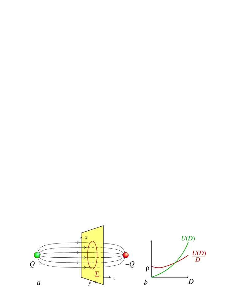
Figure 2: a) vortex spreading out over a surface $\SS$. b) Graphic calculation of the string constant $\varrho$.

So, if $U(D)/D$ has a minimum $\varrho$, preferably at some finite value of $D$ (see Fig. 2$b$), then we see that a vortex emerges, with string tension $\varrho$, spreading out more or less evenly over the surface $\SS$, while the $D$ field tends to zero outside this surface. This condition is met if $U(D)$ is linear in $D$ for small $D$ (unlike the Maxwell case, where $U(D)={\textstyle{1\over 2}}D^{2}$). In Eq. (5.4), this is realized if

$$Z(\varphi)\simeq C\cdot V(\varphi)\ ,\qquad C=2/\varrho^{2}\ ,$$ (5.6)

near the minimum of $V$.

Figure 3: $a)$ The Lagrangian $L$ as a function of the quantity $X=-{\textstyle{1\over 4}}F_{\mu\nu}F_{\mu\nu}\,$, in the case of electric confinement. The (blue) solid line shows behavior necessary for confinement. The dotted lines show different allowed continuations. $b)$ The dual of $a)$, the magnetic confinement case.

It is easy, also, to guess the effect of a possible kinetic term for $\varphi(x)$, which we had ignored. It will only contribute at the surface of this (finite size) vortex, so that the $D$ field will not show $\theta$ jumps at the edges of $\SS$, but grow more smoothly from zero outside, to the fixed value $D$ inside the vortex.

If we leave out the kinetic term for $\varphi(x)$ altogether, then we may just as well eliminate $\varphi$ from the Lagrangian (5.1) at the very beginning. Assuming Eq. (5.6) for small $V$, and $Z\simeq 1$ for large $V$ (so that the small-distance structure of the theory tends to the renormalizable situation), we find that the effective Lagrangian as a function of the entry

$$X=-{\textstyle{1\over 4}}F_{\mu\nu}F_{\mu\nu}={\textstyle{1\over 2}}\vec{E}^{2}\ ,$$ (5.7)

is obtained from the equations

$$X={{\rm d}V\over{\rm d}Z}\ ,\qquad{\cal L}(X)=ZX-V\ .$$ (5.8)

The curve is depicted in Fig. 3$a$.

The magnetic confinement case is obtained by replacing $D$ with $B$, and $Z$ with $1/Z$ in Eqs. (5.3) and (5.4). In that case, only the negative values of $X$ count, and the required behavior of the Lagrangian is depicted in Fig. 3$b$.

Investigating various functions $Z(V)$ is an instructive exercise. Further explanations can be found in Ref.[10].

References

- [1] C.G. Callan, Phys. Rev. D2 (1970) 1541; K. Symanzik, Commun. Math. Phys. 16 (1970) 48; ibid. 18 (1970) 227.
- [2] M. Gell-Mann and F. Low, Phys. Rev. 95 (1954) 1300.
- [3] D.J. Gross, in The Rise of the Standard Model, Cambridge Univ. Press (1997), ISBN 0-521-57816-7 (pbk) p. 199; H.D. Politzer, Phys. Rev. Lett. 30 (1973) 1346; D.J. Gross and F. Wilczek, Phys. Rev. Lett. 30 (1973) 1343.
- [4] G. ’t Hooft, Nucl. Phys. B61 (1973) 455; Nucl. Phys. B62 (1973) 444; see also an introductory remark on the first page of G. ’t Hooft, Nucl. Phys. B35 (1971) 167.
- [5] H.B. Nielsen and P. Olesen, Nucl. Phys. B61 (1973) 45.
-
[6]
G. ’t Hooft, Gauge Theories with Unified Weak, Electromagnetic and
Strong Interactions, in E.P.S. Int. Conf. on High Energy Physics,
Palermo, 23-28 June 1975, Editrice Compositori, Bologna 1976, A. Zichichi
Ed.;reprinted in Under the Spell of the Gauge
Principle, Adv. Series in Math. Phys., World Scientific,
1994, p. 174;
S. Mandelstam, Phys. Lett. B53 (1975) 476; Phys. Reports 23 (1978) 245. - [7] G. ’t Hooft, Phys. Scripta 24 (1981) 841; Nucl. Phys. B190 (1981) 455.
- [8] H. Georgi and S.L. Glashow, Phys. Rev. Letters 28 (1972) 1494.
- [9] G. ’t Hooft, Quarks and gauge fields, in Proceedings of the Colloqium on ”Recent Progress in Lagrangian Field Theory and Applications”, Marseille, June 24-28, 1974, ed. by C.P. Korthals Altes, E. de Rafael and R. Stora.
- [10] G. ’t Hooft, Confinement of Quarks, in Proceedings of the 16th International Conference on Particles and Nuclei (Panic’02), Osaka, Japan, Sept.-Oct., 2002, pp. 3c - 19c (Utrecht Report ITP-UU-02/65, SPIN-02/41) (to be obtained from http://www.phys.uu.nl/ thooft/gthpub.html)