210mm297mm

hep-th/0408175

UG-04/05

M-theory and Gauged Supergravities

D. Roest

Centre for Theoretical Physics, University of Groningen

Nijenborgh 4, 9747 AG Groningen, The Netherlands

E-mail: d.roest@phys.rug.nl

ABSTRACT

We present a pedagogical discussion of the emergence of gauged supergravities from M-theory. First, a review of maximal supergravity and its global symmetries and supersymmetric solutions is given. Next, different procedures of dimensional reduction are explained: reductions over a torus, a group manifold and a coset manifold and reductions with a twist. Emphasis is placed on the consistency of the truncations, the resulting gaugings and the possibility to generate field equations without an action.

Using these techniques, we construct a number of gauged maximal supergravities in diverse dimensions with a string or M-theory origin. One class consists of the $CSO$ gaugings, which comprise the analytic continuations and group contractions of $SO(n)$ gaugings. We construct the corresponding half-supersymmetric domain walls and discuss their uplift to D- and M-brane distributions. Furthermore, a number of gauged maximal supergravities are constructed that do not have an action.

Chapter 1 Introduction

This review article deals with the construction of different gauged supergravities that arise in the framework of string and M-theory. The latter are thought to be consistent theories of quantum gravity, unifying the four different forces. One of their particular features is their critical dimension: these theories necessarily live in ten or eleven dimensions. For this reason one needs a procedure to obtain effective four-dimensional descriptions, which goes under the name of Kaluza-Klein theory or dimensional reduction. In this article we will discuss a number of possible dimensional reductions and the resulting lower-dimensional descriptions. It will be useful to be acquinted with perturbative string theory (see e.g. [1, 2, 3]) and the basic concepts of string dualities (see e.g. [4, 5, 6]); in this article, emphasis will be placed on supergravity aspects.

Proposed in 1974 [7], the idea of string theory as a theory of quantum gravity was not really picked up until the "first superstring revolution" in the mid 1980s. After this period, there were five different perturbative superstring theories: four of closed strings (type IIA, IIB and heterotic with gauge group ${E_{8}\times E_{8}}$ or ${SO(32)}$) and one of open and closed strings (type I). This situation changed with the discovery of string dualities, culminating in the "second superstring revolution" in the mid 1990s. It was found that the different string theories are related to each other for different values of certain parameters; for example, the strong coupling limit of one theory yields another theory at weak coupling (S-duality) and string theories on different backgrounds are equivalent (T-duality). The upshot was that the five string theories could be unified in a single eleven-dimensional theory, which was named M-theory [8]. The different string theories are thus understood as perturbative expansions in different limits of the parameter space of M-theory. This appreciation is known as U-duality [9] and has spectacularly changed our understanding of string theory and the distinction between perturbative and non-perturbative effects.

Of central importance for the different dualities are D$p$-branes [10, 11], which are extended objects of $p$ spatial dimensions. These branes are required to fill out the multiplets of string dualities, e.g. the fundamental string is mapped onto the D$1$-brane under S-duality. In addition, different descriptions of D-branes play a crucial role in the string theory calculation [12] of the Bekenstein-Hawking entropy of a black hole and in the AdS/CFT correspondence [13], relating a string theory in a particular background (IIB on AdS₅ $\times$ S⁵) to a particular and supersymmetric QFT ($N=4$ SYM in $D=4$).

The low-energy limit of string theory, supergravity, has proven to be an important tool to study the different phenomena in string theory. Many features of string and M-theory are also present in its supergravity limit, such as D-branes and U-duality, and it is therefore interesting to study this effective description. In particular, one can extract effective lower-dimensional descriptions by considering string or M-theory on a compact internal manifold, which is taken to be very small (i.e. dimensional reduction). Different reductions give rise to different lower-dimensional supergravities. Thus it is clearly very desirable to have a proper understanding of the different reduction procedures and their resulting lower-dimensional descriptions. In particular, we will be interested in gauged supergravities as the lower-dimensional theories.

Ungauged supergravities have a global symmetry group $G$, which is a consequence of the U-duality of M-theory. In gauged supergravities a subgroup of this global group is elevated to a gauge symmetry by the introduction of mass parameters. The combination of a gauge group and local supersymmetry implies the appearance of a scalar potential, which is quadratic in the mass parameters.

It is the scalar potential which makes gauged supergravities interesting since it generically breaks the Minkowski vacuum to solutions like (Anti-)de Sitter space-time (AdS or dS), domain walls or cosmological solutions. These play important roles in the AdS/CFT correspondence and its generalisation, the DW/QFT correspondence [14, 15], brane-world scenarios [16, 17] and accelerating cosmologies [18, 19]. From various points of view, it would therefore be highly advantageous to have a classification of gauged supergravities in the different dimensions.

We are only interested, however, in gauged supergravities with a higher-dimensional origin in string or M-theory: the lower-dimensional theory must be obtainable via dimensional reduction. Our approach consists of the dimensional reduction of eleven- and ten-dimensional maximal supergravities and the investigation of the resulting gauged supergravity. We have applied two reduction methods, both preserving supersymmetry: reduction with a twist and reduction on a group manifold. In the twisted reduction one employs a global symmetry of the parent theory to induce a gauging of one of its subgroups in the lower dimension. In the group manifold reduction one reduces over a number of isometries that do not commute and form the algebra of a Lie group. This results in the gauging of this group in the lower dimension. The consistency of both reductions is guaranteed by symmetry, as proven by Scherk and Schwarz in 1979 [20, 21] and as opposed to reduction on a coset manifold, whose consistency remains to be understood in generality.

The outline of this review article is as follows. Chapter 2 is devoted to supergravity, the low-energy limit of string and M-theory. In particular, we focus on the maximal supergravities, their global symmetries and their supersymmetric solutions. In chapter 3 we describe a number of techniques to generate lower-dimensional gauged supergravities. Reduction over a torus, with a twist, over a group manifold and over a coset manifold are explained, with proper attention to the consistency of the truncation and the resulting gauging. In the last section of this chapter we discuss a subtlety which can arise for certain dimensional reductions, yielding gauged supergravities without an action. This concludes the more general part of this review.

One finds the application of the different dimensional reductions in chapter 4, where different gauged theories are constructed. By applying reductions with a twist and over a group manifold, we generate a number of gaugings in ten, nine and eight dimensions. We also discuss the class of $CSO$ gaugings in lower dimensions, which are obtainable by reduction over coset or other manifolds. Finally, in chapter 5 we construct and discuss half-supersymmetric domain wall solutions for the different gauged supergravities. The topic of the first section is the D8-brane. Next, we treat the lower-dimensional domain walls and their relation to higher-dimensional branes, with a special treatment of the 9D and 8D cases. We end with a discussion of 1/4-supersymmetric intersections of domain walls and strings.

Chapter 2 Supergravity

As mentioned in the introduction, supergravities in ten and eleven dimensions emerge as the effective low-energy description of string and M-theory. In this chapter we will discuss supersymmetry and supergravity in various dimensions, some supersymmetric solutions and their relations.

2.1 Supersymmetry

2.1.1 Superalgebra and Supercharges

The symmetry of supergravity theories is the super-Poincaré symmetry, which is an extension of the usual Poincaré symmetry of gravity theories with the generators of supersymmetry. Thus, it contains the Lorentz generators, the generators of translations (a vector under the Lorentz symmetry) and the supersymmetry generators (spinors under the Lorentz symmetry). In addition, the super-Poincaré algebra, or superalgebra in short, can be extended with a number of gauge generators, which are bosonic generators whose parameter is a $p$-form.

Due to the intertwining of the fermionic generators of supersymmetry and the bosonic generators of translations and gauge symmetries in the superalgebra, the requirement of local supersymmetry [24] has profound implications. In particular, it leads to the inclusion of gravity, due to the presence of translations in the superalgebra. Thus any locally supersymmetric theory contains gravity and is usually called a supergravity.

For the discussion of supersymmetry in $D$ dimensions we will now consider fermionic representations of the Lorentz group $SO(1,D-1)$. This is the Dirac representation and its generators are given by $[\Gamma_{\mu},\Gamma_{\nu}$], where the $\Gamma$-matrices $\Gamma_{\mu}$ satisfy the Clifford algebra

$$\{\Gamma_{\mu},\Gamma_{\nu}\}=2\eta_{\mu\nu}\,.$$ (2.1)

The dimension of this representation of the Clifford algebra is $2^{[D/2]+1}$, where the notation $[D/2]$ means the integer part of $D/2$.

Since spinors transform under the fermionic representation of the Lorentz group, their number of components in principle equals the dimension of the Dirac representation. These are called Dirac spinors. However, in certain dimensions Dirac spinors are reducible, allowing one to impose conditions that are preserved under Lorentz symmetry. For example, in even dimensions one can impose a chirality condition: spinors are required to have eigenvalue $\pm 1$ under the chirality operator

$$\Gamma_{c}=i^{D/2-1}\Gamma_{\underline{01\cdots D-1}}\,,$$ (2.2)

giving rise to Weyl spinors. In other cases it is possible to impose a reality condition, leading to Majorana spinors. In addition it is possible that both these conditions can be imposed, leading to Majorana-Weyl spinors. In table 2.1 we give the minimal spinors in different dimensions and their number of components $q$, where minimal spinors have the smallest number of components, i.e. all possible and mutually consistent conditions are imposed. A more detailed account can be found in e.g. [25, 26].

Dimension	Spinors	Components ($q$)
2 mod 8	Maj.-Weyl	$2^{D/2-1}$
3,9 mod 8	Majorana	$2^{(D-1)/2}$
4,8 mod 8	Maj. / Weyl	$2^{D/2}$
5,7 mod 8	Dirac	$2^{(D+1)/2}$
6 mod 8	Weyl	$2^{D/2}$

Table 2.1: The different minimal spinors in different space-time dimensions and their number of components. Note that one can define either Majorana or Weyl but not Majorana-Weyl spinors in $D=4,8$ mod $8$.

The parameter of supersymmetry is a spinor and thus the number of supercharges $Q$, associated to supersymmetry generators, is always a multiple $N$ of the dimension of the irreducible representation:

$$Q=Nq\,.$$ (2.3)

However, there is a bound on the number of supercharges [27]. For theories with global supersymmetry, thus not containing gravity, the bound is 16 supercharges. Theories with local supersymmetry, therefore including gravity, can have up to 32 supercharges. Superalgebras with more than 32 supercharges will only have representations that include states of helicity higher than two. When coupling these to other fields one breaks the associated gauge symmetry, thus rendering the interaction inconsistent. For this reason these higher-spin theories are usually discarded, although there are attempts to remedy the problems [28]. Theories with exactly 32 supercharges are called maximal supergravities.

Dimension	Supergravity ($N$)
11	1
10	1, IIA, IIB
7,8,9	1,2
6	1, iia, iib, 4

Table 2.2: Supergravity in different space-time dimensions, labelled by their number of supersymmetry generators.

2.1.2 Possible Supergravity Theories

When combining the bound on the number of supercharges with the dimension of the minimal spinor in the different dimensions, we can survey the different possibilities for $N$ in different dimensions, as summarised in table 2.2. One dramatic conclusion is that in dimensions twelve or higher there are no supergravity theories since the dimension of the minimum spinor is 64. Thus $D=11$ is the tip of the pyramid of supergravities, where one can only have maximal supergravity with 32 supercharges. We will discuss 11D supergravity in subsection 2.2.1.

In ten dimensions one can have either $N=1$ or $N=2$ supersymmetry, corresponding to 16 or 32 supercharges, respectively. Only the first of these cases does not necessarily contain gravity. The second case contains two Majorana-Weyl spinors of certain chiralities and thus allows for two different theories with spinors of either the opposite or the same chirality: type IIA and IIB supergravity with $(1,1)$ or $(2,0)$ supersymmetry, respectively (in this notation the first and second entries denote the number of supersymmetry generators with positive and negative chirality, respectively). In fact, $D=10$ is the only dimension which has two inequivalent maximal supergravities; it is unique in all other dimensions. We will discuss IIA and IIB supergravity in subsection 2.2.3.

The structure of maximal supergravities in ten dimensions nicely dovetails with the possible string theories with maximal supersymmetry. In ten dimensions, one has IIA and IIB string theory, whose low-energy effective actions are provided by the corresponding supergravities. For a long time, it was somewhat of a mystery what eleven-dimensional supergravity should correspond to (i.e. of which underlying theory it should be the effective action). This was clarified by the appearance of eleven-dimensional M-theory in the strong-coupling limit of IIA string theory [29, 8, 30], see also subsection 2.2.4.

Another interesting phenomenon occurs in six dimensions, where there are Weyl spinors with eight components. Of the maximal superalgebras with $N=4$, only the $(2,2)$ case gives rise to a supergravity theory; other choices contain states with higher helicity. When considering 16 supercharges, there are two choices: one finds $(1,1)$ and $(2,0)$ supersymmetry as well, leading to two distinct $Q=16$ supergravities in six dimensions, labelled iia and iib. In all other dimensions than six, the superalgebra with $Q=16$ supercharges is unique.

We would like to make a few remarks about the explicit supergravity realisation of the superalgebras. The supergravity fields form massless multiplets under supersymmetry, called supermultiplets. These are usually christened after the field with the highest helicity. The best-known example is the graviton multiplet, which includes the graviton (spin 2), the gravitino (spin 3/2) and fields with lower spin. All supergravity theories contain this multiplet. Maximal supersymmetry only allows for this supermultiplet while a smaller amount of supersymmetry allows for other multiplets without gravity as well. Examples are the gravitino and the vector multiplet with highest spins $3/2$ and $1$, respectively; see subsection 2.2.2.

Name	Symbol	Spin	On-shell d.o.f.
Graviton	$g_{\mu\nu}$	$2$	$(D-2)(D-1)/2-1$
Gravitino	$\psi_{\mu}$	$3/2$	$(D-3)\cdot q/2$
Rank-$d$ potential	$C^{(d)}_{\mu_{1}\cdots\mu_{d}}$	$1$	$\left(\;\begin{array}[]{c}D-2\\ d\end{array}\;\right)$
Dilatino	$\lambda$	$1/2$	$q/2$
Scalar	$\phi$ or $\chi$	$0$	$1$

Table 2.3: On-shell degrees of freedom of D-dimensional supergravity fields.

For supersymmetry to be a consistent symmetry, all supermultiplets must have an on-shell matching of bosonic and fermionic degrees of freedom. The on-shell degrees of freedom are multiplets of the little group $SO(D-2)$ for massless fields and are given in table 2.3 for generic supergravity fields^,. Note that a $d$-form potential $C^{(d)}$ carries the same amount of degrees of freedom as a $\tilde{d}$-form potential with $\tilde{d}=D-2-d$. What corresponds to an electric charge in one potential is a magnetic charge in its dual potential and vice versa. This equivalence between two potentials is called Hodge duality and is a generalisation of the well-known electric-magnetic duality in 4D to higher ranks $d$ and $\tilde{d}$ and dimension $D$.

2.2 Maximal Supergravities in 11D and 10D

2.2.1 Supergravity in 11D

In eleven dimensions one has maximal supersymmetry. The superalgebra allows for the inclusion of a rank-2 and a rank-5 gauge symmetry. As is always the case with maximal supersymmetry, there is only one massless supermultiplet, the graviton multiplet. It consists of the on-shell degrees of freedom

$$\text{D=11:}\qquad({\bf 44}+{\bf 84})_{\text{B}}+({\bf 128})_{\text{F}}\,,$$ (2.4)

which are multiplets of $SO(9)$. In 11D supergravity theory the graviton multiplet is usually represented by the fields

$$\text{D=11:}\qquad\{{e}_{{\mu}}{}^{{a}},{C}_{{\mu}{\nu}{\rho}};{\psi}_{{\mu}}\}\,.$$ (2.5)

These are the Vielbein, a three-form gauge potential and a Majorana gravitino, respectively. The bosonic part of the corresponding Lagrangian [31] reads

$$\mathcal{L}=\sqrt{-{g}}[{R}-\tfrac{1}{2}G\cdot G-\tfrac{1}{6}\star(G{\scriptstyle\wedge}G{\scriptstyle\wedge}C)]\,,$$ (2.6)

where ${G}=dC$. Note that it consists of the Einstein-Hilbert term, a kinetic term for the rank-three potential and a Chern-Simons term. The latter only depends on the rank-three potential and is independent of the metric; for this reason it is also called a topological term.

The 11D supergravity theory has an $\mathbb{R}^{+}$ symmetry which acts as

$$g_{\mu\nu}\rightarrow\lambda^{2}g_{\mu\nu}\,,\qquad C_{\mu\nu\rho}\rightarrow\lambda^{3}C_{\mu\nu\rho}\,,\qquad\psi_{\mu}\rightarrow\lambda^{1/2}\psi_{\mu}\,,$$ (2.7)

with $\lambda\in\mathbb{R}^{+}$. Two remarks are in order here. The above symmetry acts covariantly on the field equations (as all symmetries) but does not leave the Lagrangian invariant: it transforms as ${\cal L}\rightarrow\lambda^{9}{\cal L}$. All terms in $\cal L$ scale with the same weight: for this reason it is called a trombone symmetry [32]. Secondly, the covariant scaling of $\cal L$ only holds at lowest order. Higher-derivative corrections will scale with different weights and thus break the symmetry (2.7) of the field equations.

The occurrence of trombone symmetries will be a generic feature in ungauged or massless supergravities. The weights of the fields are always determined by a simple rule: for the bosonic fields the weights equal the number of Lorentz indices while for the fermions it is one-half less. The Lagrangian will scale as ${\cal L}\rightarrow\lambda^{D-2}{\cal L}$ under such symmetries. The scaling of bosonic terms is easily understood from the two derivatives they contain. Thus this symmetry is broken by terms with less (as in scalar potentials, to be encountered in chapter 4) or more (as in higher-order corrections) than two derivatives.

2.2.2 Minimal Supergravity in 10D

In 10D the minimal spinor is a 16-component Majorana-Weyl spinor. Minimal $N=1$ supersymmetry in 10D therefore has 16 supercharges. Its superalgebra allows for the inclusion of a rank-one and a self-dual rank-five gauge symmetry. Being non-maximal supersymmetry, one finds different supermultiplets [27]:

$$\text{N=1:}\qquad\begin{cases}\text{vector:}\qquad&({\bf 8}_{\text{v}})_{\text{B}}+({\bf 8}_{\text{c}})_{\text{F}}\,,\\ \text{graviton:}\qquad&[{\bf 8}_{\text{v}}+{\bf 8}_{\text{c}}]\times{\bf 8}_{\text{v}}=({\bf 35}_{\text{v}}+{\bf 28}+{\bf 1})_{\text{B}}+({\bf 56}_{\text{s}}+{\bf 8}_{\text{s}})_{\text{F}}\,,\\ \text{gravitino A:}\qquad&[{\bf 8}_{\text{v}}+{\bf 8}_{\text{c}}]\times{\bf 8}_{\text{s}}=({\bf 56}_{\text{v}}+{\bf 8}_{\text{v}})_{\text{B}}+({\bf 56}_{\text{s}}+{\bf 8}_{\text{s}})_{\text{F}}\,,\\ \text{gravitino B:}\qquad&[{\bf 8}_{\text{v}}+{\bf 8}_{\text{c}}]\times{\bf 8}_{\text{c}}=({\bf 35}_{\text{c}}+{\bf 28}+{\bf 1})_{\text{B}}+({\bf 56}_{\text{s}}+{\bf 8}_{\text{s}})_{\text{F}}\,,\end{cases}$$ (2.8)

Note that the little group $SO(8)$ has three 8-dimensional representations: one bosonic, the vector ${\bf 8}_{\text{v}}$, and two fermionic, spinors of opposite chirality ${\bf 8}_{\text{c}}$ and ${\bf 8}_{\text{s}}$. This special property of $SO(8)$ is known as triality.

Due to the appearance of several supermultiplets, non-maximal supergravity is not unique. It always contains the graviton multiplet, which can be coupled in various ways to vector multiplets, leading to different Yang-Mills sectors. An example is provided by the low-energy limit of the three $N=1$ string theories, which consist of the graviton multiplet plus 496 vector multiplets to obtain the $SO(32)$ or $E_{8}\times E_{8}$ gauge groups [33].

2.2.3 IIA and IIB Supergravity

Turning to maximal $N=2$ supersymmetry in 10D, one has two possibilities: one can choose Majorana-Weyl spinors of either opposite or equal chirality, leading to the non-chiral IIA or the chiral IIB supergravity theories with $(1,1)$ and $(2,0)$ supersymmetry, respectively. The IIA superalgebra can be extended with gauge symmetries of rank 0,1,2,4 and 5, while IIB allows for 1,1,3,5⁺,5⁺ and 5⁺, where all five-form gauge parameters 5⁺ are self-dual. In fact, the IIB superalgebra has an additional $SO(2)$ R-symmetry, rotating the two supersymmetry spinors of equal chirality. Under this R-symmetry, the central charges form doublets (for rank 1 and 5⁺) and singlets (for rank 3 and 5⁺). We will discuss R-symmetries of lower-dimensional superalgebras in section 2.3.

As always, maximal supersymmetry allows for only one massless multiplet, whose on-shell degrees of freedom are given by

$$\text{IIA:}\qquad[{\bf 8}_{\text{v}}+{\bf 8}_{\text{c}}]\times[{\bf 8}_{\text{v}}+{\bf 8}_{\text{s}}]=\; [({\bf 35}_{\text{v}}+{\bf 28}+{\bf 1})_{\text{NS-NS}}+({\bf 56}_{\text{v}}+{\bf 8}_{\text{v}})_{\text{R-R}}]_{\text{B}}$$

$$+[({\bf 56}_{\text{s}}+{\bf 8}_{\text{s}})_{\text{NS-R}}+({\bf 56}_{\text{c}}+{\bf 8}_{\text{c}})_{\text{R-NS}}]_{\text{F}}\,,$$

$$\text{IIB:}\qquad[{\bf 8}_{\text{v}}+{\bf 8}_{\text{c}}]\times[{\bf 8}_{\text{v}}+{\bf 8}_{\text{c}}]=\; [({\bf 35}_{\text{v}}+{\bf 28}+{\bf 1})_{\text{NS-NS}}+({\bf 35}_{\text{c}}+{\bf 28}+{\bf 1})_{\text{R-R}}]_{\text{B}}$$

$$+[({\bf 56}_{\text{s}}+{\bf 8}_{\text{s}})_{\text{NS-R}}+({\bf 56}_{\text{s}}+{\bf 8}_{\text{s}})_{\text{R-NS}}]_{\text{F}}\,,$$ (2.9)

Note that these $N=2$ supermultiplets are constructed from the $N=1$ supermultiplets: both $N=2$ graviton multiplets consist of the $N=1$ graviton and a gravitino multiplet. This is possible in 10D due to triality, which yields $N=1$ graviton and gravitino multiplets of equal size.

We will now consider the field-theoretic realisation of the graviton multiplet. The common bosonic subsector, which is called the NS-NS subsector, contains gravity, a rank-two potential and a dilaton. The remaining bosonic part is called the Ramond-Ramond subsector and will only contain R-R rank-$d$ potentials where $d$ is odd in IIA and even in IIB. The standard forms of the theories have $d=1,3$ for IIA and $d=0,2,4$ for IIB:

$$\text{IIA:}\qquad\{{g}_{{\mu}{\nu}},{B}_{\mu\nu},{\phi},C^{(1)}_{\mu},C^{(3)}_{\mu\nu\rho};{\psi}_{\mu},{\lambda}\}\,,$$

$$\text{IIB:}\qquad\{{g}_{{\mu}{\nu}},{B}_{\mu\nu},{\phi},C^{(0)},{C}^{(2)}_{\mu\nu},{C^{(4)+}_{\mu\nu\rho\sigma}};{\psi}_{\mu},{\lambda}\}\,.$$ (2.10)

In the IIA case the fermions are real and contain two minimal spinors of both chiralities, while in the IIB case they are complex and contain two minimal spinors of the same chirality. The field strength of the IIB rank-four potential $C^{(4)+}$ satisfies a self-duality constraint, halving the number of degrees of freedom.

We would also like to present a special formulation of IIA and IIB supergravity which emphasises the equivalence of dual R-R potentials, based on [34], and introduces an extra feature of IIA supergravity. To this end we will enlarge the field content by including all odd or even R-R potentials, thus allowing for the ranges $d=1,3,5,7,9$ and $d=0,2,4,6,8$. The field contents of IIA and IIB supergravity read in the double formulation

$$\text{IIA}: \qquad\{g_{\mu\nu},B_{\mu\nu},\phi,C^{(1)}_{\mu},C^{(3)}_{\mu\nu\rho},C^{(5)}_{\mu\cdots\rho},C^{(7)}_{\mu\cdots\rho};\psi_{\mu},\lambda\}\,,$$

$$\text{IIB}: \qquad\{g_{\mu\nu},B_{\mu\nu},\phi,C^{(0)},C^{(2)}_{\mu\nu},C^{(4)}_{\mu\cdots\rho},C^{(6)}_{\mu\cdots\rho},C^{(8)}_{\mu\cdots\rho};\psi_{\mu},\lambda\}\,.$$ (2.11)

To get the correct number of degrees of freedom, one must by hand impose duality relations between the field strengths of rank-$d$ and rank-$(8-d)$ potentials, which read [34]

$$G^{(d+1)}=(-)^{[(d+1)/2]}\,e^{(d-4)\phi/2}\,\star G^{(9-d)}\,,\qquad G^{(d+1)}=dC^{(d)}-H{\scriptstyle\wedge}C^{(d-2)}\,,$$ (2.12)

for vanishing fermions and where $H=dB$. The (bosonic part of the) field equations for $C^{(d)}$ can be derived from the action [34]

$$L=\sqrt{-g}[ R-\tfrac{1}{2}(\partial{\phi})^{2}-\tfrac{1}{2}e^{-\phi}H\cdot H-\sum_{d}\tfrac{1}{4}e^{(4-d)\phi/2}G^{(d+1)}\cdot G^{(d+1)}]\,,$$ (2.13)

subject to the duality relations (2.12). Due to these constraints, the above is called a pseudo-action [35]. Note that the doubling of Ramond-Ramond potentials has two effects: the kinetic terms have coefficients $1/4$ instead of the canonical $1/2$ and there are no explicit Chern-Simons terms in the action.

We would like to make the following two remarks. Note that the duality constraint on the five-form field strength of IIB can not be eliminated, in contrast to the other duality relations; it is a constraint on one field strength $G^{(5)}$ while the others relate two different field strengths $G^{(d+1)}$ and $G^{(9-d)}$ for $d\neq 4$.

Secondly, one can include a nine-form potential $C^{(9)}$ in (2.11), which carries no degrees of freedom (and thus is consistent with (2.9)) but is very natural from the point of view of R-R equivalence [11]. The corresponding field strength trivially satisfies the Bianchi identity. Its Hodge dual is a rank-zero field strength, which has no corresponding potential nor a field equation. Its Bianchi identity implies it to be constant. Thus we have effectively introduced a mass parameter in the theory, given by

$$G^{(0)}=e^{-5\phi/2}\,\star G^{(10)}\,.$$ (2.14)

The corresponding action is given by (2.13) with $d=-1,1,\ldots,9$ [34] and the field strengths [36]

$$G^{(d+1)}=dC^{(d)}-H{\scriptstyle\wedge}C^{(d-2)}+\frac{1}{(d+1)/2\,!}\,G^{(0)}B{\scriptstyle\wedge}\ldots{\scriptstyle\wedge}B\,.$$ (2.15)

Due to the equivalence of the different formulations, one should expect this mass parameter to appear in the normal formulation as well. Indeed this deformation to massive IIA supergravity has been found [37], shortly after the inception of its massless counterpart [38, 39]. In this chapter, we concentrate on the massless part and we will come back to the massive deformations in sections 4.2 and 5.1. Also, we leave the formulation with R-R equivalence here and return to the standard formulation (2.10).

The (bosonic part of the massless) IIA Lagrangian is given by

$$L_{IIA}=\sqrt{-g}[ R-\tfrac{1}{2}(\partial{\phi})^{2}-\tfrac{1}{2}e^{-\phi}H\cdot H-\sum_{d=1,3}\tfrac{1}{2}e^{(4-d)\phi/2}G^{(d+1)}\cdot G^{(d+1)}+$$

$$-\tfrac{1}{2}\star\,(dC^{(3)}{\scriptstyle\wedge}dC^{(3)}{\scriptstyle\wedge}B)]\,,$$ (2.16)

The IIA theory has two $\mathbb{R}^{+}$ symmetries. The first is a symmetry of the Lagrangian (2.16) and is given by

$$e^{\phi}\rightarrow\lambda e^{\phi}\,,\quad B_{\mu\nu}\rightarrow\lambda^{1/2}B_{\mu\nu}\,,\quad C^{(1)}_{\mu}\rightarrow\lambda^{-3/4}C^{(1)}_{\mu}\,,\quad C^{(3)}_{\mu\nu\rho}\rightarrow\lambda^{-1/4}C^{(3)}_{\mu\nu\rho}\,,$$ (2.17)

with $\lambda\in\mathbb{R}^{+}$ and other fields invariant. The other is the 10D analog of the 11D trombone symmetry (2.7) with weights as explained below the 11D weights.

The (bosonic part of the) field equations for IIB supergravity [40, 41] can be derived from the Lagrangian

$$L_{IIB}=\sqrt{-g}[ R-\tfrac{1}{2}(\partial{\phi})^{2}-\tfrac{1}{2}e^{-\phi}H\cdot H-\sum_{d=0,2,4}\tfrac{1}{2}e^{(4-d)\phi/2}G^{(d+1)}\cdot G^{(d+1)}+$$

$$+\tfrac{1}{2}\star\,(C^{(4)}{\scriptstyle\wedge}dC^{(2)}{\scriptstyle\wedge}H)]\,,$$ (2.18)

which has to be supplemented with the self-duality relation (2.12) for $d=4$ (for this reason it is called a pseudo-action [35]). The IIB supergravity theory has a global $SL(2,\mathbb{R})$ symmetry [43]

$${\tau} \rightarrow\frac{a{\tau}+b}{c{\tau}+d}\,,\quad{B}^{i}\rightarrow(\Omega^{-1})_{j}{}^{i}{B}^{j}\,,\quad C^{(4)}\rightarrow C^{(4)}\,,\quad\Omega_{i}{}^{j}=\left(\begin{array}[]{cc}a&b\\ c&d\end{array}\right)\in SL(2,\mathbb{R})\,,$$ (2.21)

$${\psi}_{{\mu}} \rightarrow\left(\frac{c\,{\tau}^{*}+d}{c\,{\tau}+d}\right)^{1/4}{\psi}_{{\mu}}\,,\quad{\lambda}\rightarrow\left(\frac{c\,{\tau}^{*}+d}{c\,{\tau}+d}\right)^{3/4}{\lambda}\,,\quad{\epsilon}\rightarrow\left(\frac{c\,{\tau}^{*}+d}{c\,{\tau}+d}\right)^{1/4}{\epsilon}\,,$$ (2.22)

where we have defined the doublet ${B}^{i}=(-B,C^{(2)})$ and the complex scalar $\tau=\chi+ie^{-\phi}$ with the axion $\chi=C^{(0)}$. In terms of the real and imaginary parts of $\tau$ the action of $SL(2,\mathbb{R})$ reads

$$e^{\phi}\rightarrow(c\chi+d)^{2}e^{\phi}+c^{2}e^{-\phi}\,,\qquad\chi\rightarrow\frac{ac+e^{2\phi}(a\chi+b)(c\chi+d)}{c^{2}+e^{2\phi}(c\chi+d)^{2}}\,,$$ (2.23)

Note that the scalars transform non-linearly. We will discuss a more covariant way to view this $SL(2,\mathbb{R})$ symmetry in section 2.3. The $SL(2,\mathbb{R})$ symmetry of IIB supergravity is broken to $SL(2,\mathbb{Z})$ in IIB string theory[9]. The element $(a,b;c,d)=(0,1;-1,0)$ corresponds to the transformation $\phi\rightarrow-\phi$ (for vanishing axion background), which relates the strong and weak string coupling. For this reason this transformation is called S-duality. In addition the IIB symmetry also has a trombone symmetry.

2.2.4 Supergravity Relations and Dualities

As we will now show, the eleven- and ten-dimensional maximal supergravity theories are not unrelated but rather can be connected via dimensional reduction. These relations can be understood from the different dualities between the different string theories and M-theory.

Ten-dimensional IIA supergravity can be obtained as a reduction of the unique supergravity theory in $D=11$. This amounts to dimensionally reducing the 11D supergravity, a procedure which is being elaborated upon in section 3.1, while only retaining the massless modes. The relations between the supergravity fields are given in (B.6). Indeed, the full 11D Lagrangian (2.6) and supersymmetry transformations (B.1) in this way give rise to the IIA counterparts (2.16) and (B.7). In terms of on-shell degrees of freedom, the 11D representations of $SO(9)$ (2.4) can be decomposed into the IIA representations of $SO(8)$ (2.9) via

$$\text{B}:\qquad{\bf 44}\rightarrow{\bf 35}_{\text{v}}+{\bf 8}_{\text{v}}+{\bf 1}\,,\qquad{\bf 84}\rightarrow{\bf 56}_{\text{v}}+{\bf 28}\,,$$

$$\text{F}:\qquad{\bf 128}\rightarrow{\bf 56}_{\text{s}}+{\bf 8}_{\text{s}}+{\bf 56}_{\text{c}}+{\bf 8}_{\text{c}}\,,$$ (2.24)

which reduces the 11D graviton multiplet to the IIA graviton multiplet.

As a side remark, from the relation (B.6) between the supergravity fields one can read off the following relations between the parameters of IIA and 11D on a circle:

$$l_{s}{}^{2}=\frac{l_{p}{}^{3}}{R}\,,\qquad g_{s}=\Big{(}\frac{R}{l_{p}}\Big{)}^{3/2}\,,$$ (2.25)

where $l_{p}$ is the 11D Planck length and $R$ the radius of the internal circle. This supports the idea that strong coupling in IIA string theory corresponds to a large radius, in which eleven-dimensional M-theory emerges. Though the appearance of eleven-dimensional Lorentz covariance can not be proven in perturbative IIA string theory (since its size is proportional to $e^{\phi}$), a lot of evidence for the existence of M-theory has been put forward [29, 8, 30]. For example, the massive Kaluza-Klein states of 11D supergravity are interpreted as the D$0$-brane states of IIA string theory [30, 44].

Similarly, IIA and IIB supergravity both reduce to the unique nine-dimensional maximal supergravity. The corresponding reduction Ansätze for the IIA and IIB supergravity fields are given in (B.14) and (B.22), respectively. These reduce the IIA and IIB supersymmetry transformations and field equations to their 9D counterparts. Also the IIA Lagrangian (2.16) can be reduced to the correct 9D action. The IIB case requires a bit more discussion due to the self-duality constraint on the 5-form field strength. Upon reduction it gives rise to a 4-form and a 5-form field strength and a duality relation between the two. The latter can be used to eliminate either of the field strengths, which is usually the 5-form. If properly treated the IIB pseudo-Lagrangian (2.18) can also be reduced to the 9D Lagrangian. In terms of on-shell degrees of freedom, the decompositions of the IIA and IIB representations of $SO(8)$ (2.9) under $SO(7)$ coincide, as can be read off explicitly:

$$\text{IIA:}\begin{cases}\text{NS-NS:}\qquad&{\bf 35}_{\text{v}}\rightarrow{\bf 27}+{\bf 7}+{\bf 1}\,,\qquad{\bf 28}\rightarrow{\bf 21}+{\bf 7}\,,\qquad{\bf 1}\rightarrow{\bf 1}\,,\\ \text{R-R}:\qquad&{\bf 56}_{\text{v}}\rightarrow{\bf 35}+{\bf 21}\,,\qquad\quad\;{\bf 8}_{\text{v}}\rightarrow{\bf 7}+{\bf 1}\,,\\ \text{NS-R:}\qquad&{\bf 56}_{\text{s}}\rightarrow{\bf 48}+{\bf 8}\,,\qquad\quad\quad{\bf 8}_{\text{s}}\rightarrow{\bf 8}\,,\\ \text{R-NS:}\qquad&{\bf 56}_{\text{c}}\rightarrow{\bf 48}+{\bf 8}\,,\qquad\quad\quad{\bf 8}_{\text{c}}\rightarrow{\bf 8}\,,\\ \end{cases}$$

$$\text{IIB:}\begin{cases}\text{NS-NS:}\qquad&{\bf 35}_{\text{v}}\rightarrow{\bf 27}+{\bf 7}+{\bf 1}\,,\qquad{\bf 28}\rightarrow{\bf 21}+{\bf 7}\,,\qquad{\bf 1}\rightarrow{\bf 1}\,,\\ \text{R-R}:\qquad&{\bf 35}_{\text{c}}\rightarrow{\bf 35}\,,\qquad\qquad\;\quad\;{\bf 28}\rightarrow{\bf 21}+{\bf 7}\,,\qquad{\bf 1}\rightarrow{\bf 1}\,,\\ \text{NS-R:}\qquad&{\bf 56}_{\text{s}}\rightarrow{\bf 48}+{\bf 8}\,,\qquad\quad\quad{\bf 8}_{\text{s}}\rightarrow{\bf 8}\,,\\ \text{R-NS:}\qquad&{\bf 56}_{\text{s}}\rightarrow{\bf 48}+{\bf 8}\,,\qquad\quad\quad{\bf 8}_{\text{s}}\rightarrow{\bf 8}\,,\end{cases}$$ (2.26)

Thus the massless modes of IIA and IIB supergravity on $S^{1}$ are equivalent and indeed are described by the same effective theory, the unique $D=9$ maximal supergravity.

However, the massive modes of IIA and IIB supergravity on $S^{1}$, sometimes called momentum modes, are distinct. For this reason, IIA and IIB supergravity are only equivalent on very small circles, where such modes become infinitely massive (for more detail, see section 3.1). String theory modifies this situation in the following way. Due to the fact closed strings can wind around the internal direction, there is an entire tower of massive winding multiplets. Note that this phenomenon is intrinsic to string theory and does not have a counterpart in field theory. It turns out that the combination of massive momentum states and massive winding states yields the same result for IIA and IIB string theory; to be precise, IIA on a circle with radius $R$ is equivalent to IIB on a circle with radius $\tilde{R}$ with the relation $\tilde{R}=\alpha^{\prime}/R$ [10, 45]. Such a relation between theories on different compactification manifold is generically called T-duality [46]. The towers of momentum and winding states are interchanged under the T-duality transformation on $S^{1}$. In accordance with their accompanying string theories, the map between the (dimensionally reduced) IIA and IIB supergravities is usually called T-duality.

The strong coupling limit of IIB string theory can be understood from its conjectured $SL(2,\mathbb{Z})$ symmetry [9]. Indeed, this symmetry is shared by its low-energy approximation and one of its generators acts on the IIB supergravity fields as $\phi\rightarrow-\phi$ (for vanishing axion background). This corresponds to a strong-weak coupling transformation due to the interpretation of the dilaton and is called S-duality. For this reason, IIB string theory is understood to be self-dual. At weak coupling, strings are the fundamental, perturbative degrees of freedom while at strong coupling, this role is played by the D$p$-branes with $p=1$.

2.3 Scalar Cosets and Global Symmetries in $D\leq 9$

We now turn to the remaining maximal supergravities in $D\leq 9$. Being unique these can all be obtained by dimensional reduction of any of the higher-dimensional theories, in the same way that IIA supergravity can be obtained from 11 dimensions. Their construction is rather straightforward and we will not consider it in great detail. One aspects deserves proper discussion however: the scalar sector and its transformation under the global symmetries of the theory. See [49] for a clear discussion.

2.3.1 Scalar Cosets

The field content of any $D\leq 9$-dimensional maximal supergravity is easily obtained by dimensional reduction; its bosonic subsector consisting of gauge potentials is given in table 2.4. The same holds for the Lagrangians and general formulae for maximal supergravity in any dimension have been obtained [50]. The bosonic part generically reads

$${\cal L}_{D}=\sqrt{-g}[R-\tfrac{1}{2}(\partial\vec{\phi})^{2}-\sum_{d,i}\tfrac{1}{2}e^{\vec{\alpha}_{d}^{i}\cdot\vec{\phi}}G^{(d+1)}_{i}\cdot G^{(d+1)}_{i}]+{\cal L}_{CS}\,,$$ (2.27)

where the $G^{(d+1)}_{i}$ are rank-$(d+1)$ field strengths of gauge potentials $C^{(d)}_{i}$ with $d=0,\ldots,3$. The index $i$ denotes the different $d$-form potentials; its range can be inferred from table 2.4. The number of dilatons $\vec{\phi}$ always equals $11-D$ since all reduced dimensions will give rise to one dilaton. The length of the vectors $\vec{\alpha}_{d}^{i}$ will always be given by

$$\vec{\alpha}_{d}^{i}\cdot\vec{\alpha}_{d}^{i}=4-\frac{2d(D-d-2)}{D-2}\,,$$ (2.28)

in maximal supergravity.

Of special interest in this Lagrangian is the scalar sector, which we rewrite as

$${\cal L}_{\text{scalars}}=\sqrt{-g}[-\tfrac{1}{2}(\partial\vec{\phi})^{2}-\sum_{i}\tfrac{1}{2}e^{\vec{\alpha}^{i}\cdot\vec{\phi}}G^{(1)}_{i}\cdot G^{(1)}_{i}]\,.$$ (2.29)

where $G^{(1)}_{i}$ are the one-form field strengths of the axions $\chi^{i}$ and where we have dropped the subscript $0$ on the vectors $\vec{\alpha}^{i}$. The vectors $\vec{\alpha}^{i}$ can be interpreted as positive root vectors of a simple Lie algebra. In the Cartan-Weyl basis, the generators of this algebra are the Cartan generators $\vec{H}$, the positive root generators $E_{\vec{\alpha}^{i}}$ and the negative root generators $E_{-\vec{\alpha}^{i}}$ with commutation relations

$$[\vec{H},\vec{H}]=0\,,\qquad[\vec{H},E_{\vec{\alpha}^{i}}]=\vec{\alpha}^{i}E_{\vec{\alpha}^{i}}\,,\qquad[E_{\vec{\alpha}^{i}},E_{\vec{\alpha}^{j}}]=N(\vec{\alpha}^{i},\vec{\alpha}^{j})E_{\vec{\alpha}^{i}+\vec{\alpha}^{j}}\,,$$ (2.30)

and similarly for the negative root generators (replacing $\vec{\alpha}^{i}\rightarrow-\vec{\alpha}^{i}$). The coefficients $N(\vec{\alpha}^{i},\vec{\alpha}^{j})$ are constants (possibly zero) and characterise the algebra. We will now show that the scalar sector (2.29) is invariant under the action of the corresponding semi-simple group $G$.

To this end we construct a particular representative of $G$, defined by

$$L=\text{exp}(\sum_{i}\chi^{i}E_{\vec{\alpha}^{i}})\text{exp}(-\vec{\phi}\cdot\vec{H}/2)\,,$$ (2.31)

with parameters $\vec{\phi}$ corresponding to the Cartan generators and $\chi^{i}$ to the positive root generators. This parameterises the coset $G/H$ with $H$ the maximal compact subgroup of $G$. The group $H$ will turn out to be the R-symmetry group of the superalgebra. Upon acting with a group element $g\in G$ from the left, the element $gL$ will generically no longer have the form of the $G/H$ representative (2.31), i.e. this can in general not be expressed as a transformation $\vec{\phi}\rightarrow\vec{\phi}^{\prime}$ and $\chi^{i}\rightarrow{\chi^{i}}^{\prime}$. However, one can employ the Iwasawa decomposition, which states that

$$L\rightarrow gL=L^{\prime}h\,,$$ (2.32)

i.e. the resulting matrix can be decomposed as $L^{\prime}$ of the form (2.31) and a remainder $h\in H$. The latter will be dependent on $\vec{\phi}$ and $\chi^{i}$ in general. Due to the Iwasawa decomposition we have defined a transformation

$$L(\vec{\phi},\chi^{i})\rightarrow L^{\prime}=gL(\vec{\phi},\chi^{i})h^{-1}=L(\vec{\phi}^{\prime},{\chi^{i}}^{\prime})\,,$$ (2.33)

consisting of a left-acting $G$ element and a compensating right-acting $H$ element. Note that for global $G$ transformations, the action of $H$ will be local due to the field dependence via $\vec{\phi}$ and $\chi^{i}$. The $H$ transformation is called compensating since it compensates for the $G$ transformation that does not preserve the $G/H$ representative (2.31).

The relevance of the transformation properties of $L$ stems from the fact that the scalar kinetic terms (2.29) can be written as

$${\cal L}_{\text{scalars}}=\sqrt{-g}[\tfrac{1}{4}\text{Tr}(\partial M\partial M^{-1})]\,,$$ (2.34)

where we have defined $M=LL^{T}$. Note that $M$ does not see the compensating $H$ transformation: it transforms as $M\rightarrow gMg^{T}$ under (2.33). Thus the scalar sector is by construction invariant under global $G$ transformations. It turns out that this group is a symmetry not only of the scalar subsector but of the entire theory, i.e. when also including the potentials of higher rank and the fermions.

Let us take a step back and consider the significance of the compensating transformation $H$. We have shown that the scalar kinetic terms (2.29) are invariant under the global symmetry $G$ by constructing a particular $G/H$ representative $L$. Every $G$ transformation is accompanied by a compensating $H$ transformation to keep $L$ of the same form. This can be seen as the gauge fixed version (with gauge choice (2.31)) of a more covariant system with global $G$ and local $H$ symmetry. The covariant system has kinetic term (2.34) for arbitrary $L\in G$. The extra degrees of freedom that are introduces in $L$ are cancelled by the extra gauge degrees of freedom $L\rightarrow Lh$ with $h\in H$ local. This is a completely equivalent formulation of the scalar sector with advantages due to its covariance.

2.3.2 Example: $SL(2,\mathbb{R})$ Symmetry of IIB

To make matters more concrete let us discuss the scalar sector of IIB supergravity as an example. From its Lagrangian one reads off that it has one dilaton and one axion with positive root vector $\alpha=2$. This corresponds to the simple Lie algebra $sl(2)$ with generators (in the fundamental representation)

$$H=\left(\begin{array}[]{cc}1&0\\ 0&-1\end{array}\right)\,,\qquad E_{+2}=\left(\begin{array}[]{cc}0&1\\ 0&0\end{array}\right)\,,\qquad E_{-2}=\left(\begin{array}[]{cc}0&0\\ 1&0\end{array}\right)\,,$$ (2.41)

satisfying the algebra (2.30). Next we define the $SL(2,\mathbb{R})/SO(2)$ representative

$$L=e^{\chi E_{+2}}e^{-\phi H/2}=\left(\begin{array}[]{cc}e^{-\phi/2}&e^{\phi/2}\chi\\ 0&e^{\phi/2}\end{array}\right)\,.$$ (2.44)

Any left-acting $SL(2,\mathbb{R})$ transformation on $L$ can be compensated by a right-acting field-dependent $SO(2)$ transformation. Indeed one can easily identify these in the explicit $SL(2,\mathbb{R})$ transformations (2.22) of IIB supergravity. The two-form potentials transform linearly under $G$ while the fermions only transform under the compensating $SO(2)$ transformations. Without gauge fixing the $G$ transformations would read (omitting $SL(2,\mathbb{R})$ indices)

$$L \rightarrow g\,L\,h_{SO(2)}^{-1}\,,\qquad {B} \rightarrow(g^{-1})^{T}{{B}}\,,\qquad C^{(4)} \rightarrow C^{(4)}\,,$$

$${\psi}_{{\mu}} \rightarrow h_{U(1)}^{1/2}{\psi}_{{\mu}}\,,\qquad {\lambda} \rightarrow h_{U(1)}^{3/2}{\lambda}\,,\qquad {\epsilon} \rightarrow h_{U(1)}^{1/2}{\epsilon}\,.$$ (2.45)

where $g$ and $h$ are given by

$$g=\left(\begin{array}[]{cc}a&b\\ c&d\end{array}\right)\in SL(2,\mathbb{R})\,,\quad h_{SO(2)}=\text{exp}\left(\begin{array}[]{cc}0&\theta(x)\\ -\theta(x)&0\end{array}\right)\,,\quad h_{U(1)}=\text{exp}(i\theta(x))\,.$$ (2.50)

This clearly shows the two different symmetries that act independently in the covariant formulation. The gauge fixing condition translates in the role of $H$ as compensating transformation with

$$\theta=-\text{arccos}\left(\frac{e^{\phi}(c\chi+d)}{\sqrt{c^{2}+e^{2\phi}(c\chi+d)^{2}}}\right)\,.$$ (2.51)

Indeed, the transformations $\eqref{IIBSL2Rcov}$ with constraint (2.51) reduce to the non-linear transformations (2.22).

2.3.3 Global Symmetries of Maximal Supergravities

Having dealt with the simplest example in $D=10$, we now turn to lower-dimensional scalar cosets. In table 2.4 we give the groups $G$ and $H$ that one encounters. The groups $G$ are symmetries of 11D supergravity on a torus; it is expected that $G$ is broken to an arithmetic subgroup $G(\mathbb{Z})$ for the full M-theory on a torus [9].

The dimension of the scalar coset $G/H$ equals the number of scalars; the number of axions is given by the number of positive roots of the algebra corresponding to $G$ while the number of dilatons equals $11-D$ (one for every reduced dimension). In table 2.4 we also give the bosonic potentials of higher rank and their transformation under the $G$ groups. The potentials form linear representations of $G$ while they are invariant under $H$. We do not give the fermionic field content; see e.g. [26]. In contrast to the bosons, the fermions are invariant under $G$ but transform under $H$. One can check these statements in the example of $SL(2,\mathbb{R})$ symmetry in IIB supergravity, see (2.22) and (2.45).

$D$	G	H	Dim$[G/H]$	$d=1$	$d=2$	$d=3$	$d=4$
$11$	$1$	$1$	$-$	$-$	$-$	$\bf 1$	$-$
IIA	$\mathbb{R}^{+}$	$1$	$1$	$\bf 1$	$\bf 1$	$\bf 1$	$-$
IIB	$SL(2,\mathbb{R})$	$SO(2)$	$2$	$-$	$\bf 2$	$-$	${\bf 1}^{+}$
$9$	$SL(2,\mathbb{R})\times\mathbb{R}^{+}$	$SO(2)$	$3$	${\bf 2}+{\bf 1}$	$\bf 2$	$\bf 1$	$-$
$8$	$\begin{array}[]{c}SL(3,\mathbb{R})\times\\ \times SL(2,\mathbb{R})\end{array}$	$\begin{array}[]{c}SO(3)\times\\ \times SO(2)\end{array}$	$7$	$\bf(3,2)$	$\bf(3,1)$	${\bf(1,2)}^{+}$	$-$
$7$	$SL(5,\mathbb{R})$	$SO(5)$	$14$	$\bf 10$	$\bf 5$	$-$	$-$
$6$	$SO(5,5)$	$SO(5)\times SO(5)$	$25$	$\bf 16$	${\bf 10}^{+}$	$-$	$-$
$5$	$E_{6(+6)}$	$USp(8)$	$42$	$\bf 27$	$-$	$-$	$-$
$4$	$E_{7(+7)}$	$SU(8)$	$70$	${\bf 56}^{+}$	$-$	$-$	$-$

Table 2.4: The groups $G$ and $H$ and the $d$-form gauge potentials as representations of $G$ of maximal supergravity in $6\leq D\leq 11$. The $+$ denotes self-dual representations: there are duality constraints that halve the number of degrees of freedom. In all but the IIB case the constraints can be eliminated at the cost of breaking manifest $G$ covariance.

Note that the global symmetry group $G$ in $D$ dimensions is often larger than the $SL(11-D,\mathbb{R})$ that is expected from the connection with eleven-dimensional supergravity (as will be explained in subsection 3.2.2). For this reason, the group $G$ is known as a hidden symmetry [51, 52, 53]. Another important feature in even dimensions is that they are only symmetries of the equations of motion and not of the Lagrangian. For example, this can come about when the symmetry transformation involves a Hodge dualisation of a gauge potential, which can only be performed straightforwardly on the field equations and not on the Lagrangian. This is the origin of the self-dual representations in table 2.4.

A number of complications turn up in $D\leq 5$, as can be inferred from table 2.4. First of all, the exceptional groups of the A-D-E-classification (of simply-laced simple Lie algebras) appear. Secondly, one needs to dualise potentials of higher rank to axions to realise the symmetry group $G$. Also the $H$ groups are no longer orthogonal and one needs a generalised notion of orthogonality. Some details can be found in [54].

The appearing symmetry groups $G$ can be represented by Dynkin diagrams. Here each node represents a simple root (spanning the space of positive roots) and the number of lines (zero, one, two or three) between two nodes corresponds to an angle of 90, 120, 135 or 150 degrees between the associated simple roots. In the algebras that we encounter all simple root vectors have the same length (simply laced algebras) and angles of 120 degrees with respect to each other. The Dynkin diagrams of maximal supergravity are distilled into figure 2.1. Indeed, continuation to $D<6$ brings one to the exceptional Lie algebras.

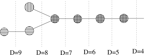
Figure 2.1: The Dynkin diagrams of the symmetry groups $G$ of maximal supergravity in different dimensions summarised in one picture. Given $D$, the part to the left of the corresponding split is relevant. The horizonal and vertical fillings correspond to the 11D and IIB origin, respectively.

Note that the Dynkin diagram is very reminiscent of the possible maximal supergravities; with a highest node in 11D, two possibilities in 10D and unique possibilities in $D\leq 9$. Indeed, one can view the symmetry group $G$ as coming from the higher-dimensional origin: reduction over a $d$-torus gives rise to an $SL(d,\mathbb{R})$ symmetry (as explained in subsection 3.2.2). Thus, one can understand the horizontally filled nodes as coming from 11D while the vertical fillings come from IIB. Together, these two subgroups generate the full duality group $G$ in any dimension $D\leq 9$ [55].

As an amusing note we would like to mention that the same phenomenon occurs in $Q=16$ supergravity. As discussed in subsection 2.1.2, these are unique in all dimensions but six, where one encounters non-chiral iia and chiral iib, similar to IIA and IIB in $D=10$. Again, the existence of this extra supergravity in six dimensions gives rise to an extra $SL(2,\mathbb{R})$ symmetry in four dimensions.

However, despite many similarities, the above discussion does not directly carry over to theories with less supersymmetry. For example, the global symmetry group $G$ is always maximally non-compact for the case of maximal supersymmetry. In less supersymmetric cases this is not necessarily true, in which case one should not exponentiate all Cartan generators but only the non-compact ones. Some of these issues are discussed in [49].

2.4 Supersymmetric Solutions

2.4.1 Generic Brane Solutions

In the previous sections we have seen that supergravity theories generically contain bosonic fields of spin 0,1 and 2, corresponding to a scalar, a rank-$d$ potential and the graviton. In this subsection we will take a step back and discuss generic solutions to this system called $p$-brane solutions. These are generalisations of the extremal Reissner-Nordström charged black hole to $d\neq 1$ (the rank of the gauge potential) and $D\neq 4$ (the dimension of space-time). These will occur frequently as supersymmetric solutions of supergravities, as we will find below. For reviews see e.g. [56, 57].

The starting point is the D-dimensional toy model Lagrangian

$$\mathcal{L}=\sqrt{-g}[R-\tfrac{1}{2}(\partial\phi)^{2}-\tfrac{1}{2}e^{a\phi}G^{(d+1)}\cdot G^{(d+1)}]\,,$$ (2.52)

with the rank-$(d+1)$ field strength $G^{(d+1)}=dC^{(d)}$. It consists of an Einstein-Hilbert term, a dilaton kinetic term and a kinetic term for a rank-$d$ potential with arbitrary dilaton coupling, parameterised by $a$. For future use we define the constants [58]

$$\Delta=a^{2}+\frac{2d\tilde{d}}{D-2}\,,\qquad\tilde{d}=D-d-2\,.$$ (2.53)

The constant $\Delta$ will play an important role in the characterisation of solutions. In particular, in many supergravities it will be given by $4/n$ with $n$ a positive integer and the corresponding $p$-brane solutions will preserve a fraction $1/2^{n}$ of the supersymmetry.

Due to the presence of the gauge potential, solutions to this system can carry electric and magnetic charge, defined by

$$Q_{e}=\int_{S^{\tilde{d}+1}}e^{a\phi}\star G^{(d+1)}\,,\qquad Q_{m}=\int_{S^{d+1}}G^{(d+1)}\,.$$ (2.54)

These are conserved due to the field equation of $C^{(d)}$ and the Bianchi identity of $G^{(d+1)}$, respectively, and can be seen as generalisations of the Maxwell charges in 4D. Hodge dualisation interchanges the electric and magnetic charges since the dual field strengths are related by (in analogy to (2.12))

$$e^{a\phi}G^{(d+1)}=\star{G}^{(\tilde{d}+1)}\,,$$ (2.55)

where ${G}^{(\tilde{d}+1)}=d{C}^{(\tilde{d})}$. Under this dualisation the field equations for $C^{(d)}$ is transformed to the Bianchi identity for the dual field strength ${G}^{(\tilde{d}+1)}$ while the Bianchi identity for $G^{(d+1)}$ corresponds to the field equation for the dual potential ${C}^{(\tilde{d})}$. Also $\Delta$ is invariant under Hodge dualisation since this interchanges $d$ and $\tilde{d}$ and flips the sign of $a$.

The system (2.52) allows for two $p$-brane solutions, where $p$ refers to the dimensionality of the spatial extension of the brane, that carry one of the charges (2.54):

electric $$p \qquad p=d-1\,,$$-brane:

magnetic $$p \qquad p=\tilde{d}-1\,.$$-brane:

The dimension of the world-volume equals $p+1$ while the remainder $D-p-1$ is the dimension of the transverse space and is called the codimension.

We will discuss the electric and magnetic $p$-brane solutions at the same time. To this end, we split up the coordinates in the world-volume $t,x^{i}$ with $i=1,\ldots,p$ and the transverse space $x^{m}$ with $m=p+1,\ldots,D-1$. The metric and dilaton are given by

$$ds^{2} =H^{-4\tilde{d}/(\Delta(D-2))}(-dt^{2}+dx_{i}{}^{2})+H^{4d/(\Delta(D-2))}dx_{m}{}^{2}\,,\quad e^{\phi}=H^{\pm 2a/\Delta}\,,$$ (2.56)

where the electric and magnetic solutions have a $+$ and a $-$ sign, respectively. The corresponding field strengths are given by^,

$$G^{(d+1)}_{e}=\frac{2}{\sqrt{\Delta}}\,dt{\scriptstyle\wedge}dx^{1}{\scriptstyle\wedge}\cdots{\scriptstyle\wedge}dx^{p}{\scriptstyle\wedge}dH^{-1}\,,\quad G^{(d+1)}_{m}=\frac{2}{\sqrt{\Delta}}\star(dt{\scriptstyle\wedge}dx^{1}{\scriptstyle\wedge}\cdots{\scriptstyle\wedge}dx^{p}{\scriptstyle\wedge}dH)\,.$$ (2.57)

The $p$-branes are characterised by the function $H(x^{m})$, which is given by (for the moment we assume $p<D-3$; we will discuss the other cases later)

$$H=c+\frac{Q}{r^{D-p-3}}\,,$$ (2.58)

with $r=\|x^{m}\|$. The integration constants $c$ and $Q$ are taken both positive to avoid naked singularities at finite $r$. All such $p$-brane solutions have $ISO(1,p)\times SO(D-p-1)$ isometry. For branes with $a\neq 0$ the constant $c$ can be related to the asymptotic value of $\phi$ via $g_{s}=\exp(\phi)_{\infty}=c^{\pm 2a/\Delta}$.

The $p$-brane solutions have a horizon at $r=0$. Depending on $D$, $p$ and $\Delta$ the horizon may coincide with a singularity or it may be possible to find a geodetically complete extension of the solution. We will not pursue the solution behind the horizon and will content ourselves with the description of the $0<r<\infty$ part of space-time, thus avoiding the possible necessity for a source term. This part interpolates between two different vacua of the theory [59]: one finds D-dimensional Minkowski space for $r\rightarrow\infty$ and a metric which is conformal to a product of Anti-de Sitter space and a higher-dimensional sphere:

$$ds^{2}=H^{2a^{2}/(\Delta(D-p-3))}(ds^{2}(AdS_{p+2})+ds^{2}(S^{D-p-2}))\,,$$ (2.59)

for $r\rightarrow 0$, which is called the near-horizon limit.

The $p$-brane solutions carry mass and charge density. The ADM mass per unit $p$-brane volume is given by

$$M=\frac{4Q(D-p-3)g_{s}^{-a/2}\Omega_{D-p-2}}{\sqrt{\Delta}}\,,$$ (2.60)

where $\Omega_{D-p-2}$ is the volume of the unit $(D-p-2)$-sphere that surrounds the $p+1$-dimensional world-volume. Computing the charge densities from (2.54), one finds that there is an equality between the mass and (the absolute value of) the charge density: $M=|Q_{e}|$ for the electric solution and $M=|Q_{m}|$ for the magnetic solution. In supergravity theories this will generically lead to an amount of preserved supersymmetry.

There are several generalisations of the prime examples (2.56), (2.57) of $p$-brane solutions. For instance, one can replace the function $H=H(x^{m})$ by any solution to the Laplace equation

$$\Box H(x^{m})=\partial_{n}\partial^{n}H(x^{m})=0\,,$$ (2.61)

in $(D-p-1)$-dimensional flat transverse space. Examples are

• the multi-center $p$-brane solution with

  $$H=c+\sum_{i}\frac{Q_{i}}{\|x^{m}-x_{i}^{m}\|^{D-p-3}}\,,$$ (2.62)

  with all $Q_{i}$ positive to avoid naked singularities at finite $x^{m}$. Its interpretation consists of a number of $p$-branes located at $x_{i}^{m}$. Physically, this solution is possible since all separate $p$-branes have equal mass and charge; for this reason their attractive force (due to gravity and the scalar) cancels their repulsive force (due to the rank-$d$ potential).

• the smeared $p$-brane solution with $H=H(x^{m})$ a harmonic function in a subspace of the full transverse space. An example is the following function for $p<D-4$:

  $$H=c+\frac{Q}{\|x^{\tilde{m}}\|^{D-p-4}}\,,$$ (2.63)

  where $\tilde{m}=p+1,\ldots,D-2$, i.e. the harmonic function does not depend on $x^{D-1}$. This can be interpreted as the configuration of a smooth distribution of $p$-brane in the $x^{D-1}$-direction. The smeared solutions will be very relevant later for the relation between the different solutions.

These generalisations break part of the isometry group. However, since the mass and charge of these solutions are still equal, they will preserve supersymmetry in a supergravity theory.

It is also possible to add mass to the $p$-brane solution without affecting its charge: $Q_{e,m}<M$. This generically breaks the supersymmetry and (part of the) isometry of the solutions. For example, one can construct non-supersymmetric solutions with isometry group $\mathbb{R}\times ISO(p)\times SO(D-p-1)$ [61, 62]. Such deformations are only possible for the single-center solution (2.58) and not for its multi-center generalisation (2.62), as can physically be understood from the inequality of mass and charge: the attractive and repulsive forces between different constituents no longer cancel.

2.4.2 Branes with Little Transverse Space

Let us now discuss branes with $p\geq D-3$, starting with the case that saturates this bound. Such branes are sometimes called vortex branes and have a two-dimensional transverse space. The most symmetric harmonic function reads (with $r=\|x^{m}\|$)

$$H=c+Q\log(r)\,,$$ (2.64)

giving rise to $ISO(1,D-3)\times SO(2)$ isometry. The limit $r\rightarrow\infty$ in this case does not yield D-dimensional Minkowski but an asymptotically locally flat space-time; locally this is Minkowski but a global difference occurs in the form of a deficit angle in the 2D transverse space, stemming from the mass density of the $(D-3)$-brane solution. The other limit, $r\rightarrow 0$, is not well-defined since the harmonic function becomes negative at finite $r$, thus rendering this solution valid only for $r$ large enough. However, there are modifications of this solution with the same large-$r$ behaviour and a well-defined interior [63].

The next case concerns $(D-2)$-branes which are usually referred to as domain walls. Their transverse space is one-dimensional, on which the most general harmonic function reads (where $y=x^{D-1}$)

$$H=c+Qy\,,$$ (2.65)

where we take $Q$ positive. Note that a potential of rank $D-1$, corresponding to an electric domain wall, carries no degrees of freedom (see table 2.3). Its Hodge dual

$${G}^{(0)}=e^{a\phi}\star G^{(D)}=2Q/\sqrt{\Delta}\,,$$ (2.66)

is a constant zero-form field strength and can be interpreted as a mass parameter. We thus find that mass parameters can support domain walls. A necessary condition for this is the quadratic term in (2.52) with $d=0$. Rather than a kinetic term it is called a scalar potential (due to the coupling to the dilaton) and its form determines the possible properties of domain wall solutions. We will encounter many examples of scalar potentials in gauged supergravities, see chapter 4.

Again, one might wonder if the domain wall solution interpolates between different vacua. Due to the one-dimensional transverse space, the domain walls differ in this respect from the other $p$-branes. One can always do a reparameterisation of the transverse coordinate [64] to obtain the metric of either conformal Anti-de Sitter space-time or of conformal Minkowski space-time. However, the domain wall as it stands is certainly not a globally well-defined solution: one finds that the harmonic function vanishes for finite $y$. To remedy the resulting singularity, one has to patch solutions with different values for the mass parameters. This requires the presence of source terms, whose charge is related to the difference between the values of the mass parameters on both sides of the domain wall. We will discuss an example of such a source term in section 5.1.

Domain walls of the above type are usually called thin domain walls: the source term corresponds to a object of infinitesimal thickness in the transverse direction. Such source terms are always necessary with potentials of the form (2.52) with $p=D-2$, which have only one asymptotic minimum (with $\phi\rightarrow\pm\infty$). In contrast, potentials with more than one (local) minima allow for solutions interpolating between two minima. Such smooth configurations are called thick domain walls. We will mostly encounter the thin version in this article, however.

Taking the $p$-brane classification one step further by considering $p=D-1$ brings us to space-time-filling branes. All of space-time is world-volume and there is no transverse space. Though not very interesting from a supergravity point of view there is an appreciation of space-time filling branes in string theory [11, 65].

2.4.3 Maximally Supersymmetric Solutions

In section 2.2 we have encountered different supergravity theories in eleven and ten dimensions. In the next two subsections we will discuss solutions of these theories that preserve a fraction of supersymmetry.

From the supersymmetry transformations one can deduce which solutions can preserve supersymmetry. We will only consider bosonic solutions. For these to preserve supersymmetry, the right-hand side of the supersymmetry transformations of the fermions must vanish. These conditions are the Killing spinor equations. Here one distinguishes two possibilities: either all terms in the variation of the fermions vanish separately, leading to maximally supersymmetric solutions, or there is a cancellation between non-zero terms. The latter case will involve a condition on the supersymmetry parameter $\epsilon$ due to the different $\Gamma$-structures. The supersymmetry parameter subject to this condition is called the Killing spinor. Since it is constrained this will lead to solutions preserving only fractions of supersymmetry.

All maximally supersymmetric solutions to maximal supergravity in eleven and ten dimensions have been classified [66]. Minkowski space-time without field strengths is a maximally supersymmetric solution to 11D, IIA and IIB supergravity. In addition to this trivial vacuum, there are so-called AdS $\times$ S and plane wave solutions that preserve all supersymmetry. The AdS $\times$ S metric consists of a product of a $(d+1)$-dimensional Anti-de Sitter space-time and an $(D-d-1)$-dimensional sphere, whose isometry group is $SO(1,d+1)\times SO(D-d)$ (which is considerably larger than that of the brane solutions with rank-$(d+1)$ field strengths). In addition, there is a flux of the rank-$(d+1)$ field strength though the sphere. In eleven dimensions one has such solutions with $d=3$ and $d=6$ [67, 68] while IIB allows for the $d=4$ case. The plane wave solution, found in 11D [69] and in IIB [70], has the metric of a gravitational plane wave and a constant null flux of the rank-four and self-dual rank-five field strength, respectively. Only recently has it been appreciated [71] that the maximally supersymmetric plane wave is the Penrose limit [72, 73] of the AdS $\times$ S solutions.

2.4.4 Half-supersymmetric Solutions

The solutions preserving half supersymmetry have also received a lot of attention. Here the Killing spinor is subject to a projection:

$$\tfrac{1}{2}(1\pm O)\epsilon=\epsilon\,,\qquad O^{2}=1\,.$$ (2.67)

The possible projectors of 11D, IIA and IIB supergravity are given in table 2.5. Each theory has a number of $p$-brane solutions while they have the plane wave and Kaluza-Klein monopole in common.

$O$	11D, IIA, IIB solution	$O$	11D solution
$\Gamma_{\underline{01}}$	pp-wave	$\Gamma_{\underline{012}}$	M2-brane
$\Gamma_{\underline{1234}}$	Kaluza-Klein monopole	$\Gamma_{\underline{12345}}$	M5-brane
$O$	IIA solution	$O$	IIB solution
$\Gamma_{\underline{0}}\Gamma_{11}$	D0-brane	$\text{i}\Gamma_{\underline{01}}\star$	D1-brane
$\Gamma_{\underline{01}}\Gamma_{11}$	F1-brane	$\Gamma_{\underline{01}}\star$	F1-brane
$\Gamma_{\underline{012}}$	D2-brane	$\Gamma_{\underline{01234}}\star$	D3-brane
$\Gamma_{\underline{12345}}$	D4-brane	$\text{i}\Gamma_{\underline{1234}}\star$	D5-brane
$\Gamma_{\underline{1234}}\Gamma_{11}$	NS5-brane	$\Gamma_{\underline{1234}}\star$	NS5-brane
$\Gamma_{\underline{123}}\Gamma_{11}$	D6-brane	$\text{i}\Gamma_{\underline{12}}$	D7-brane

Table 2.5: Possible projection operators of the supersymmetry transformations of 11D, IIA and IIB supergravity and the corresponding half-supersymmetric solutions.

The branes of table 2.5 are labelled by their value of $p$, which equals $d-1$ for the electric solution and $\tilde{d}-1=D-d-3$ for the magnetic solution. Their metric, dilaton and field strength are given in (2.56) and (2.57). In addition, their values of $a$ (the dilaton coupling to the field strength kinetic term in the electric formulation) can be read off from (2.6), (2.16) and (2.18):

• $a=0$ for the M-branes [74, 75],

• $a=-1$ for the F1-brane [76],

• $a=\tfrac{1}{2}(3-p)$ for the D-branes [61],

• $a=+1$ for the NS5-brane [77].

From (2.53) it follows that these branes all have $\Delta=4$. Such branes preserve half of supersymmetry. Note that $a$ vanishes for the M2-, M5- and D3-brane. This has an important consequence: their near-horizon limits (2.59) are of the form $AdS^{4}\times S^{7}$, $AdS^{7}\times S^{4}$ and $AdS_{5}\times S^{5}$ (without conformal factor), respectively, which are maximally supersymmetric vacua of 11D and IIB supergravity. Thus one finds isometry and supersymmetry enhancement in the near-horizon limit for these branes.

We can now interpret the brane solutions of IIA and IIB supergravity in the context of string theory. An important tool will be the dependence of the mass on the coupling constant $g_{s}$, which is given by

$$M\sim g_{s}^{-(2a+p+1)/4}\,.$$ (2.68)

The F1-solution corresponds to the fundamental string, which is charged with respect to the NS-NS 2-form $B$. Its mass scales like $g_{s}{}^{0}$. The D$p$-brane solutions are interpreted as the $p+1$-dimensional hyperplanes on which open strings can end [78], due to imposition of so-called Dirichlet boundary conditions. These carry charge of the corresponding R-R potential $C^{(p+1)}$ and their masses scale as $1/g_{s}$, which is in between fundamental and solitonic behaviour. The microscopic understanding of D-branes in terms of open strings with Dirichlet boundary conditions was one of the key insights that led to the second superstring revolution. Note that the remaining brane solution, the NS5-brane, has a mass that scales like $1/g_{s}{}^{2}$ and can thus be considered truly solitonic.

In addition to the brane solutions one has so-called pp-wave solutions. Its metric and field strength read (in light-cone coordinates $x^{\pm}=t\pm x^{1}$ and $x^{m}$ with $m=2,\ldots,D-1$):

$$ds^{2}=2dx^{+}dx^{-}+H(x^{m},x^{-})(dx^{-})^{2}+(dx^{m})^{2}\,,\qquad G^{(d+1)}=dx^{-}{\scriptstyle\wedge}\xi^{(d)}\,,$$ (2.69)

where $H$ and $\xi^{(d)}$ satisfy the requirements

$$\Box H=-\tfrac{1}{4}\|\xi^{(d)}\|^{2}\,,\qquad d\xi^{(d)}=d\star\xi^{(d)}=0\,,$$ (2.70)

which are all defined on the transverse Euclidean space with coordinates $x^{m}$ (for all $x^{-}$). The field strength $G^{(d+1)}$ can be the four-form field strength of 11D or several field strengths of IIA and IIB. This pp-wave solution generically preserves half supersymmetry (with the projector as given in table 2.5) but special choices of $H$ and $\xi^{(d)}$ give rise to more supersymmetry [79, 80, 81, 82]. For 11D and IIB one obtains maximal supersymmetry for the truncation to the plane wave

11D: $$\begin{cases}\xi^{(3)}=\mu dx^{2}{\scriptstyle\wedge}dx^{3}{\scriptstyle\wedge}dx^{4}\,,\\ H(x^{m},x^{-})=-\tfrac{1}{9}\mu^{2}((x^{2})^{2}+(x^{3})^{2}+(x^{4})^{2})-\tfrac{1}{36}\mu^{2}((x^{5})^{2}+\cdots+(x^{10})^{2})\,,\end{cases}$$

IIB: $$\begin{cases}\xi^{(4)}=\mu dx^{2}{\scriptstyle\wedge}dx^{3}{\scriptstyle\wedge}dx^{4}{\scriptstyle\wedge}dx^{5}+\mu dx^{6}{\scriptstyle\wedge}dx^{7}{\scriptstyle\wedge}dx^{8}{\scriptstyle\wedge}dx^{9}\,,\\ H(x^{m},x^{-})=-4\mu^{2}((x^{2})^{2}+\cdots+(x^{9})^{2})\,.\end{cases}$$ (2.71)

Another special case is the Brinkmann wave [83], a purely gravitational solution with $\xi^{(d)}=0$. It is described in terms of one harmonic function, i.e. a function satisfying $\Box H=0$. There is in general no supersymmetry enhancement for this case.

Another purely gravitational solution of 11D, IIA and IIB is provided by the Kaluza-Klein monopole [84, 85] ($m=1,2,3$ and $i=5,\ldots,D-1$):

$$ds^{2}=-dt^{2}+dx_{i}^{2}+H^{-1}(dx^{4}+A_{m}dx_{m})^{2}+Hdx_{m}^{2}\,,$$ (2.72)

where the functions $H=H(x^{m})$ and $A_{m}=A_{m}(x^{n})$ are subject to the condition

$$F_{mn}=\tfrac{1}{2}(\partial_{m}A_{n}-\partial_{n}A_{m})=\varepsilon_{mnp}\partial_{p}H\,.$$ (2.73)

This metric is the product of a Minkowski space-time and the 4D Euclidean Taub-NUT space with isometry direction $x^{4}$. The $SO(3)$ isometric case is given by (where $r=\|x^{m}\|$)

$$H=c+\frac{Q}{r}\,.$$ (2.74)

This gives rise to a regular geometry if the isometry direction $x^{4}$ is compact with period $4\pi Q$ [86]. Its near-horizon limit $r\rightarrow 0$ gives rise to flat space-time and thus indeed gives rise to both isometry and supersymmetry enhancement. In addition to the $SO(3)$ isometric case, one can take also take multi-centered solutions or smeared versions, as discussed in 2.4.1. The Kaluza-Klein monopole also preserves half of supersymmetry for generic choices of the harmonic function.

2.4.5 Relations between Half-Supersymmetric Solutions

The above solutions constitute all known maximally and half-supersymmetric solutions of eleven- and ten-dimensional maximal supergravity. Since the theories in 10D and 11D are related to each other upon dimensional reduction, as we found in subsection 2.2.4, one can also relate their solutions. One provision is that the solution must have the correct isometry to allow for this reduction. Reduction in a transverse direction is therefore only possible for smeared solutions with harmonic functions that have an extra isometry. Reduction in a world-volume direction is always possible. Thus, reduction of the two M-branes gives rise to four different brane solutions of IIA supergravity. Similar remarks hold for the relations between IIA and IIB solutions.

Figure 2.2: The web of half-supersymmetric solutions and their relations in D=10 and D=11 maximal supergravities. Solid lines correspond to dimensional reduction or T-duality, the dashed lines correspond to S-duality. If an arrow ends with a head, the operation leads to the maximally isometric solution; if not, one obtains a smeared version. Adapted from [65].

In figure 2.2 we show the relations between the different solutions that preserve half of supersymmetry. Note that the solutions in the NS-NS sectors of IIA and IIB transform into each other; the same holds for the D-branes of the R-R sectors. As for the pp-wave solutions, we have only considered their purely gravitational limit (the gravitational wave) since the solution is then expressible in terms of a harmonic function, which greatly simplifies the T-duality discussion.

Furthermore, solutions with less than 1/2 supersymmetry have been studied extensively. For example, it has been known for long that 11D supergravity allows for solutions preserving 1/4 or 1/8 supersymmetry [75]. Only later these were understood as intersections of different solutions preserving 1/2 supersymmetry [87]. A lot of intersections have been studied since, see [88] for a review.

Chapter 3 Dimensional Reduction

As discussed in the introduction, the most promising candidates for quantum gravity are M- and string theory. It is of interest to investigate which four-dimensional effective descriptions can be obtained from these ten- and eleven-dimensional theories. As a first step, in this chapter we will discuss the techniques of extracting different effective descriptions from a higher-dimensional field theory.

3.1 Introduction

3.1.1 Scalar Field and Kaluza-Klein States

Consider a complex scalar field $\hat{\phi}$ in $\hat{D}$ dimensions, depending on the coordinates $x^{\hat{\mu}}=(x^{\mu},z)$. One can expand the dependence on one of the coordinates via the Fourier decomposition:

$$\hat{\phi}(x,z)=\int dke^{ikz}\phi_{k}(x)\,,$$ (3.1)

in terms of components $\phi_{k}$ with momentum $k$. If, in addition, the $z$ direction is taken to be compact of length $2\pi R$ and we impose the boundary condition $\hat{\phi}(x,0)=\hat{\phi}(x,2\pi R)$, the integral becomes the sum

$$\hat{\phi}(x,z)=\sum_{n}e^{inz/R}\phi_{n}(x)\,,$$ (3.2)

over a discrete spectrum of fields $\phi_{n}$ with momentum $k=n/R$ in the compact direction.

Suppose the complex scalar $\hat{\phi}$ is subject to the Klein-Gordon equation $\hat{\Box}\hat{\phi}=0$ where $\hat{\Box}=\partial_{\mu}\partial^{\mu}+\partial_{z}\partial^{z}$. Upon inserting the Fourier transform in this equation, one obtains separate equations for components with different momentum:

$$\Box\phi_{k}-k^{2}\phi_{k}=\Box\phi_{n}-(n/R)^{2}\phi_{n}=0\,,$$ (3.3)

where $\Box=\partial_{\mu}\partial^{\mu}$. This is the equation for a scalar of (mass)² $k^{2}$ or $(n/R)^{2}$. Thus a massless scalar in $\hat{D}$ dimensions splits up in an infinite number of scalar fields in $D=\hat{D}-1$ dimensions. In the context of dimensional reduction, these are called Kaluza-Klein states. Only one of these (the component $\phi_{0}$) is massless, while the other ones are massive. The spectrum of Kaluza-Klein states is continuous for a non-compact internal direction and discrete for $z$ compact. The latter spectrum therefore has a mass gap, which is an important ingredient when considering compactifications.

3.1.2 Consistency of Truncations

The fact that one obtains separate equations for the different Fourier components lies at the heart of dimensional reduction. First one expresses a higher-dimensional field in an infinite tower of lower-dimensional fields by expanding the dependence on the internal coordinates into harmonics on the internal manifold. Next, one observes that one can consistently truncate to a finite number of fields and set the rest of the spectrum equal to zero. Here, a consistent truncation refers to the origin in the higher-dimensional theory: every lower-dimensional solution should uplift to a higher-dimensional one.

Usually, one truncates to only the massless sector for the following reason. In dimensional reduction the masses are inversely proportional to the size of the internal manifold (as can be seen on dimensional grounds and in the example (3.3)). Since we live in an effectively four-dimensional world, any internal directions must be very small. This means that the mass of states with non-zero momentum becomes very large. Therefore, these modes are too massive to be physically interesting and are usually discarded. In the above example, this would correspond to keeping only $\phi_{0}$ and truncating the other components.

Note however that one does not need to take a very small size of the internal manifold for the massive modes to decouple; in many cases it is always a consistent truncation to retain only the massless modes, irrespective of whether the internal manifold is small or large or indeed, whether it is compact or non-compact. Again, the scalar field serves as an example: the Klein-Gordon equation for $\hat{\phi}$ splits up in many lower-dimensional equations, which are all solved by $\Box\phi_{0}=0$ and $\phi_{k}=0$ (in the non-compact case) or $\phi_{n}=0$ (in the compact case). Thus any solution to the equation for $\phi_{0}$ will also solve the higher-dimensional Klein-Gordon equation for $\hat{\phi}$.

Another important point is that the lower-dimensional degrees of freedom are not always massless. In such cases, the Fourier expansion of a field over the internal manifold does not comprise any massless fields. A consistent truncation then only keeps the lightest modes of a field. The set of lower-dimensional fields then do not have the same mass: some may be massless (such as gravity and gauge vectors) while others are massive (such as scalars). In the above discussion of consistent truncation, this corresponds to replacing massless with lightest.

In the reduction procedures that we consider in this chapter, the number of degrees of freedom is unchanged by the dimensional reduction: every higher-dimensional degree of freedom corresponds, after the expansion and truncation, to one lower-dimensional degree of freedom. These lower-dimensional fields fall in multiplets of the isometry group of the internal manifold. In particular, when expanding a theory including gravity over a manifold with isometry group $G$, one expects non-Abelian gauge vectors of $G$ to be among the massless lower-dimensional modes, see e.g. [89]. This will be an essential feature in sections 3.4 and 3.5.

Thus dimensional reduction consists of an expansion over an internal manifold and a subsequent truncation to the lightest subsector. However, this is usually not what is done in practice. Rather, a reduction Ansatz is constructed, relating higher-dimensional fields to a set of lower-dimensional fields. This is the result of the expansion and truncation: the lower-dimensional fields are the lightest modes of the expansion. Dimensional reduction then consists of substituting the reduction Ansatz in the field equations or Lagrangian. In many cases the reduction Ansatz contains a certain dependence on the internal coordinates. To be able to interpret the resulting equations as a lower-dimensional theory, this dependence should cancel at the end of the day. This requirement is equivalent to the consistency of truncations to the finite number of lower-dimensional fields.

In this chapter we will consider toroidal and twisted reductions and reductions over group and coset manifolds, all of which are consistent reductions. In the case of toroidal reduction, the reduction Ansatz is taken independent of the internal coordinates $z^{m}$. Toroidal reduction is therefore obviously consistent. The other three reductions require a certain $z^{m}$-dependence. For reductions with a twist and over a group manifold, the cancellation of the internal coordinate dependence is guaranteed on group-theoretical grounds, as will be explained in sections 3.3 and 3.4. In the remaining reduction over a coset manifold this cancellation is quite miraculous and poorly understood; it has been proven only in a small number of cases, see section 3.5. Examples of reductions whose consistency (in the above sense) has not been proven are Calabi-Yau compactifications, which we will not consider.

3.2 Toroidal Reduction

In this section we will consider the reduction Ansätze for toroidal reduction of gravity, gauge potentials and fermions. As indicated above, for reduction over a torus one does not include dependence on the internal coordinates and thus its consistency is guaranteed. More information can be found in e.g. [49].

3.2.1 Gravity on a Circle

We will now consider the reduction of gravity in $\hat{D}$ dimensions over a circle to $D=\hat{D}-1$ dimensions. To this end, the coordinates are split up according to $x^{\hat{\mu}}=(x^{\mu},z)$. We will use the following choice for the decomposition of $\hat{D}$-dimensional gravity into $D$-dimensional fields:

$$\hat{ds}^{2}=e^{2\alpha\phi}ds^{2}+e^{2\beta\phi}(dz+A_{\mu}dx^{\mu})^{2}\,,$$ (3.4)

i.e. gravity decomposes into a lower-dimensional gravity plus a vector $A_{\mu}$ and a scalar $\phi$. The constants $\alpha$ and $\beta$ are in principle arbitrary. This Ansatz gives rise to a lower-dimensional theory with the Lagrangian

$$\mathcal{L}=\sqrt{-\hat{g}}\hat{R}=\sqrt{-g}[R-\tfrac{1}{2}(\partial\phi)^{2}-\tfrac{1}{2\,2!}e^{2(\beta-\alpha)\phi}F^{2}]\,,$$ (3.5)

with $F=dA$. Here we have chosen the constants to the values

$$\alpha^{2}=\frac{1}{2(D-1)(D-2)}\,,\qquad\beta=-(D-2)\alpha\,,$$ (3.6)

to obtain the lower-dimensional Lagrangian in the conventional form (3.5), i.e. without dilaton coupling for the Ricci scalar and with the factor $\tfrac{1}{2}$ in the dilaton kinetic term. Note that this a system of the form that was considered in subsection 2.4.1 on brane solutions, with parameter $\Delta$ as defined in (2.53) equal to $4$ for all dimensions $D$.

The appearance of the Maxwell kinetic term was the reason for Kaluza [90] and Klein [91] to consider such dimensional reductions: it seemed possible to unify gravity and electromagnetism in 4D by the introduction of a fifth coordinate. Note however that there is also an extra scalar, which can not be simply set equal to zero: this would be inconsistent with the higher-dimensional field equations. Often these extra fields are called the Kaluza-Klein scalar and vector. Also, the general procedure of obtaining a lower-dimensional description from a higher-dimensional theory is sometimes called Kaluza-Klein theory. We will not use this terminology, however, since we need to make a distinction between the different possibilities within Kaluza-Klein theory.

One can understand the lower-dimensional symmetries of the Lagrangian (3.5) by considering its higher-dimensional origin. In particular, the $\hat{D}$-dimensional Einstein-Hilbert action is invariant under general coordinate transformations

$$\delta x^{\hat{\mu}}=-\hat{\xi}^{\hat{\mu}}\,,\qquad\Rightarrow\delta\hat{g}_{\hat{\mu}\hat{\nu}}=\hat{\xi}^{\hat{\rho}}\partial_{\hat{\rho}}\hat{g}_{\hat{\mu}\hat{\nu}}+\hat{g}_{\hat{\rho}\hat{\nu}}\partial_{\hat{\mu}}\hat{\xi}^{\hat{\rho}}+\hat{g}_{\hat{\mu}\hat{\rho}}\partial_{\hat{\nu}}\hat{\xi}^{\hat{\rho}}\,.$$ (3.7)

In general, such a transformation will not preserve the form of the reduction Ansatz (3.4), i.e. the resulting metric will not be expressible as (3.4) with transformed fields. The Ansatz will only transform covariantly under transformations with specific parameters. Such Ansatz-preserving transformations and their effect on the lower-dimensional fields are the following:

$$\delta x^{\mu}=-\xi^{\mu}(x)\,,\qquad \Rightarrow\begin{cases}\delta g_{\mu\nu}=\xi^{\rho}\partial_{\rho}g_{\mu\nu}+g_{\rho\nu}\partial_{\mu}\xi^{\rho}+g_{\mu\rho}\partial_{\nu}\xi^{\rho}\,,\\ \delta A_{\mu}=\xi^{\rho}\partial_{\rho}A_{\mu}+A_{\rho}\partial_{\mu}\xi^{\rho}\,,\\ \delta\phi=\xi^{\rho}\partial_{\rho}\phi\,,\end{cases}$$

$$\delta z=-\lambda(x)\,,\qquad \Rightarrow\begin{cases}\delta A_{\mu}=\partial_{\mu}\lambda\,,\end{cases}$$

$$\delta z=-cz\,,\qquad \Rightarrow\begin{cases}\delta g_{\mu\nu}=-2\alpha cg_{\mu\nu}/\beta\,,\\ \delta A_{\mu}=-cA_{\mu}\,,\\ \delta\phi=c/\beta\,.\end{cases}$$ (3.8)

These can respectively be understood as $D$-dimensional general coordinate transformations, $U(1)$ gauge transformations and a global scale symmetry.

The latter can be integrated to give a finite, rather than infinitesimal, transformation. In addition one has the higher-dimensional trombone symmetry $\hat{g}_{\hat{\mu}\hat{\nu}}\rightarrow\lambda^{2}\hat{g}_{\hat{\mu}\hat{\nu}}$, which also reduces to a finite scale symmetry of the lower-dimensional theory. One can construct linear combinations of these symmetries to obtain the following transformations

$$g_{\mu\nu}\rightarrow\lambda_{1}{}^{2}g_{\mu\nu}\,,\qquad A_{\mu}\rightarrow\lambda_{1}A_{\mu}\,,$$ (3.9)

where $\lambda_{1}\in\mathbb{R}^{+}$. This is the lower-dimensional trombone symmetry (with coefficients as explained in subsection 2.2.1), which scales all terms in the Lagrangian with the same factor, and is only a symmetry of the field equations. The other combination reads

$$A_{\mu}\rightarrow\lambda_{2}{}^{\alpha-\beta}A_{\mu}\,,\qquad e^{\phi}\rightarrow\lambda_{2}e^{\phi}\,,$$ (3.10)

also with $\lambda_{2}\in\mathbb{R}^{+}$. This corresponds to the only scale symmetry of the Lagrangian. Indeed, this explains the two $\mathbb{R}^{+}$ symmetries of IIA supergravity: they stem from combinations of the 11D trombone symmetry and internal coordinate transformations.

3.2.2 Gravity on a Torus

The reduction of gravity over a torus $T^{n}$ can be seen as successive reductions over $n$ circles. The reduction Ansatz of $\hat{D}$-dimensional gravity over an $n$-torus to $D=\hat{D}-n$ dimensions reads (with a coordinate split $x^{\hat{\mu}}=(x^{\mu},z^{m})$ where $m=1,\ldots,n$)

$$\hat{ds}^{2}=e^{2\alpha\phi}ds^{2}+e^{2\beta\phi}M_{mn}(dz^{m}+A^{m}_{\mu}dx^{\mu})(dz^{n}+A^{n}_{\mu}dx^{\mu})\,.$$ (3.11)

The lower-dimensional field strength is a generalisation of the result of a torus reduction: in addition to gravity one finds $n$ vectors $A^{m}_{\mu}$, a dilaton $\phi$ and a scalar matrix $M_{mn}$ which parameterises a coset $SL(n,\mathbb{R})/SO(n)$ (see section 2.3 for scalar cosets). The latter corresponds to $n-1$ dilatons and $\tfrac{1}{2}n(n-1)$ axions. Again, one can obtain the lower-dimensional Lagrangian by a reduction of the Einstein Hilbert term:

$$\mathcal{L}=\sqrt{-\hat{g}}\hat{R}=\sqrt{-g}[R-\tfrac{1}{2}(\partial\phi)^{2}+\tfrac{1}{4}\text{Tr}(\partial M\partial M^{-1})-\tfrac{1}{2\,2!}e^{2(\beta-\alpha)\phi}M_{mn}F^{m}F^{n}]\,,$$ (3.12)

with $F^{m}=dA^{m}$. The convenient values for $\alpha$ and $\beta$ now read

$$\alpha^{2}=\frac{n}{2(D+n-2)(D-2)}\,,\qquad\beta=-\frac{(D-2)\alpha}{n}\,,$$ (3.13)

yielding the Lagrangian in the conventional form (3.12).

As in the reduction over the circle, one can wonder which general coordinate transformations (3.7) preserve the form of the reduction Ansatz and induce a lower-dimensional transformation. For the torus reduction (3.11) these turn out to be

$$\hat{\xi}^{\mu}=\xi^{\mu}(x)\,,\qquad\hat{\xi}^{m}=\lambda^{m}(x)+\Lambda^{m}{}_{n}z^{n}\,.$$ (3.14)

These can respectively be understood as $D$-dimensional general coordinate transformations, $U(1)^{n}$ gauge transformations and a global $GL(n,\mathbb{R})$ symmetry. As in the torus case, the global transformations can be integrated to finite transformations, where it is convenient to use a split into $SL(n,\mathbb{R})$ and $\mathbb{R}^{+}$. The former acts in the obvious way on the $SL(n,\mathbb{R})$ indices while the latter can again be combined with the reduced trombone symmetry to yield the lower-dimensional trombone symmetry and the dilaton scale symmetry (formulae (3.9) and (3.10) with an extra $m$ index for $A_{\mu}$). Thus, in comparison with the circle case, the new features of the $n$-torus reduction are the $n$ Abelian gauge symmetries and the global $SL(n,\mathbb{R})$ symmetry.

3.2.3 Inclusion of Gauge Potentials

We will now consider the reduction of a gauge potential of rank $d$ over a circle. The dynamics of the higher-dimensional potential $\hat{C}^{(d)}$, coupled to gravity and possibly a dilaton $\hat{\varphi}$, is determined by

$$\mathcal{L}=\sqrt{-\hat{g}}[-\tfrac{1}{2}(\partial\hat{\varphi})^{2}-\tfrac{1}{2}e^{a\hat{\varphi}}\hat{G}^{(d+1)}\cdot\hat{G}^{(d+1)}]\,.$$ (3.15)

with $\hat{G}^{(d+1)}=d\hat{C}^{(d)}$, where we have included the dilaton kinetic term. The parameter $a$ characterises the dilaton coupling. For gravity we will take the reduction Ansatz (3.4) while the rest of the reduction Ansatz reads

$$\hat{C}^{(d)}=C^{(d)}+(dz+A){\scriptstyle\wedge}C^{(d-1)}\,,\qquad\hat{\varphi}=\varphi\,.$$ (3.16)

where $A$ is the Kaluza-Klein vector field of the gravity Ansatz (3.4). The resulting Lagrangian is described by

$$\mathcal{L}=\sqrt{-{g}}[-\tfrac{1}{2}({\partial}{\varphi})^{2}-\tfrac{1}{2}e^{a{\varphi}-2d\alpha\phi}{G}^{(d+1)}\cdot{G}^{(d+1)}-\tfrac{1}{2}e^{a{\varphi}+2(D-d-1)\alpha\phi}G^{(d)}\cdot{G}^{(d)}]\,,$$ (3.17)

with field strengths ${G}^{(d+1)}=d{C}^{(d)}+F{\scriptstyle\wedge}C^{(d-1)}$ and ${G}^{(d)}=d{C}^{(d-1)}$. Note that $\Delta$, defined in (2.53), is preserved under the operation of dimensional reduction; the value associated to $\hat{G}^{(d+1)}$ is also found for both ${G}^{(d+1)}$ and ${G}^{(d)}$:

$$\Delta =a^{2}+\frac{2d(\hat{D}-d-2)}{\hat{D}-2}\,,$$

$$=a^{2}+(2d\alpha)^{2}+\frac{2d(D-d-2)}{D-2}\,,$$

$$=a^{2}+(2(D-d-1)\alpha)^{2}+\frac{2(d-1)(D-d-1)}{D-2}\,.$$ (3.18)

Indeed, this corresponds to the statement from subsection 2.4.1 that the parameter $\Delta$ is invariant under toroidal reduction.

The reduction of a $d$-form gauge potential over a circle can be performed a number of times. This corresponds to the reduction over a torus. We will not discuss the explicit Ansatz here since it follows from (3.16) but clearly there are general formulae for the reduction of a gauge potential over a torus, similar to (3.11). However, it is useful to know the resulting field content. From subsequent applications of (3.16) it can be seen that the reduction of a $d$-form over an $n$-torus gives rise to an amount of

$$\left(\begin{array}[]{c}n\\ d-\tilde{d}\end{array}\right)\,,\qquad\text{where\leavevmode\nobreak\ \leavevmode\nobreak\ }d-n\leq\tilde{d}\leq d\,,$$ (3.21)

forms of rank $\tilde{d}$. For example, reduction of a $2$-form over a $2$-torus gives rise to a $2$-form, two vectors and a scalar.

Upon reduction over a torus, the gauge symmetry $\delta\hat{C}^{(d)}=d\hat{\lambda}^{(d-1)}$ splits up in different lower-dimensional gauge transformations, corresponding to the different $\tilde{d}$-form potentials. In the case of a circle, for example, the gauge transformations that act covariantly on the lower-dimensional potentials are

$$\hat{\lambda}^{(d-1)}=\lambda^{(d-1)}+(dz+A){\scriptstyle\wedge}\lambda^{(d-2)}\,,$$ (3.22)

where $A$ is the Kaluza-Klein vector. The gauge parameters $\lambda^{(d-1)}$ and $\lambda^{(d-2)}$ correspond to the potentials $C^{(d)}$ and $C^{(d-1)}$, respectively.

In addition, the higher-dimensional Lagrangian is of course invariant under the general coordinate transformations (3.7). As in the case of gravity, the reduction Ansatz for gauge potentials over a torus is only covariant for the restricted transformations (3.14). The lower-dimensional potentials transform in the usual way under the lower-dimensional coordinate transformations and they can also be assigned a weight under the global scale symmetries. Moreover, the $\tilde{d}$-form potentials, the number of which is given by (3.21), form linear representations of the global $SL(n,\mathbb{R})$ symmetry.

3.2.4 Global Symmetry Enhancement

However, this is not the full story of gravity and gauge potentials on tori. It turns out that, in special cases, one obtains a larger symmetry group than the $SL(n,\mathbb{R})$ whose appearance was guaranteed by the higher-dimensional coordinate transformations. An obvious example is provided by the Lagrangian (3.5), which is the reduction of the Einstein-Hilbert action over a circle. Reduction of (3.5) over an $n$-torus will lead to the global symmetry $SL(n+1,\mathbb{R})$ rather than $SL(n,\mathbb{R})$. In this case one can understand the symmetry enhancement by the higher-dimensional origin of (3.5). However, there are also examples where such an explanation is not available.

As an example, consider the bosonic string, whose low-energy limit consists of gravity, a dilaton and a rank-two gauge potential. After appropriate field redefinitions, the action takes the canonical form (2.52) of the gravity-dilaton-potential system of subsection 2.4.1, with a dilaton coupling corresponding to $\Delta=4$. Upon reduction over an $n$-torus, it turns out that the global symmetry group is enhanced from $SL(n,\mathbb{R})$ to $SO(n,n)$, see e.g. [26]. In addition, the scalar coset is enhanced as well:

$$\frac{SL(n,\mathbb{R})}{SO(n)}\qquad\Rightarrow\qquad\frac{SO(n,n)}{SO(n)\times SO(n)}\,.$$ (3.23)

For this to be possible, there is a conspiracy between the scalars coming from the metric (giving rise to the smaller coset) and those coming from the two-form, together giving rise to the larger coset.

Another example is provided by the reduction of (the bosonic sector of) eleven-dimensional supergravity, whose symmetry groups are given in table 2.4. Again, the symmetry groups and scalar cosets are larger than the naive $SL(n,\mathbb{R})$. In this case this requires a collaboration between the scalars coming from the metric and those coming from the three-from gauge potential. Although often appearing in the low-energy limits of string or M-theory, it should be stressed that such symmetry enhancement is a miraculous phenomenon and strongly dependent on the details of interactions.

3.2.5 Fermionic Sector

If one wants to dimensionally reduce a supergravity theory, clearly a recipe is required for the fermionic sector. Since this is rather strongly dependent on the dimensions of the higher- and lower-dimensional theories, we will not present explicit formulae but only discuss the conceptual aspects. In the explicit reduction of supergravities that we will perform later, such explicit formulae are given while in this chapter however, we will mainly consider the bosonic part. For more detail see e.g. [89, 49].

The essential idea in fermionic dimensional reduction is to split up the spinors as a tensor product of spinors in the lower-dimensional space and the internal space. For toroidal reduction, the internal spinors are taken constant. Thus, the reduction Ansatz for a dilatino sketchily reads

$$\hat{\lambda}=\sum_{i}\lambda^{i}\otimes\eta^{i}\,,$$ (3.24)

where $\lambda^{i}$ are the lower-dimensional spinors and $\eta^{i}$ the internal spinors. The range of $i$ is equal to the number of independent spin-$1/2$ components on the internal manifold and therefore strongly depends on $\hat{D}-D$. This range corresponds to the quotient of the degrees of freedom of the minimal spinors in the higher- and lower-dimensional theory. For example, reducing over a seven-torus, the $32$-component minimal spinor $\hat{\lambda}$ splits up in $4$-component minimal spinors $\lambda^{i}$ and therefore $i$ ranges from $1$ to $8$. This corresponds for example to the reduction of $N=1$ supergravity in 11D to $N=8$ supergravity in 4D over the seven-torus, which indeed allows for eight constant internal spinors.

In the case of spin-$3/2$ fermions, i.e. if the fermions are carrying a space-time index as well, the procedure is a combination of the bosonic and fermionic Ansätze. Both spinorial and space-time indices are split up into the lower-dimensional ranges:

$$\hat{\psi}_{\mu}=\sum_{i}\psi_{\mu}^{i}\otimes\eta^{i}\,,\qquad\hat{\psi}_{m}=\sum_{j}\lambda^{j}\otimes\eta_{m}^{j}\,,$$ (3.25)

where $\eta^{i}$ and $\eta_{m}^{j}$ are constant fermions on the internal space of spin 1/2 and 3/2, respectively. Thus the resulting fermions are the gravitini $\psi_{\mu}^{i}$ and the dilatini $\lambda^{j}$.

We will indicate the changes in the fermionic Ansätze in the upcoming cases of twisted reduction and reductions over group manifolds.

3.3 Reduction with a Twist

We will now discuss a generalisation of toroidal reduction, leading to a different lower-dimensional description including e.g. a scalar potential. This generalisation is possible whenever the higher-dimensional theory contains a global symmetry [20].

3.3.1 Boundary Conditions and Twisted Expansions

In subsection 3.1.1 we considered the expansion of a complex scalar field over an internal dimension under the assumption $\hat{\phi}(x,2\pi R)=\hat{\phi}(x,0)$, i.e. a periodic boundary condition. One can also impose the generalised boundary condition

$$\hat{\phi}(x,2\pi R)=e^{2\pi imR}\hat{\phi}(x,0)\,,$$ (3.26)

for some constant $m$. We will call this the twisted boundary condition, giving rise to reduction with a twist. It leads to the expansion

$$\hat{\phi}(x,z)=\sum_{n}e^{i(m+n/R)z}\phi_{n}(x)\,,$$ (3.27)

with a discrete spectrum of fields $\phi_{n}$. Note that this twisted expansion is invariant under the transformation

$$m\rightarrow m+1/R\,,\qquad\phi_{n}\rightarrow\phi_{n+1}\,.$$ (3.28)

For this reason one can always take $|m|\leq\tfrac{1}{2}/R$ without loss of generality. Substitution into the Klein-Gordon equation yields

$$\Box\phi_{n}-(m+n/R)^{2}\phi_{n}=0\,.$$ (3.29)

Again, the higher-dimensional equation decouples into separate equations for all components $\phi_{n}$ of (mass)² $(m+n/R)^{2}$.

Again, we would like to truncate to the sector with the lowest mass; to which component $\phi_{n}$ this corresponds to is determined by the parameter $m$. Adhering to the above convention of taking $|m|\leq\tfrac{1}{2}/R$, the lowest sector corresponds to the component $\phi_{0}$, as in the massless case. Note however that the lower-dimensional description is different; the periodic boundary condition gave rise to a massless scalar while the twisted boundary condition leads to a scalar of (mass)² $m^{2}$. However, both reductions are consistent: the field equations for $\phi_{n}$ with $n\neq 0$ are satisfied and, equivalently, the dependence on the internal coordinate $z$ has dropped out.

Note that one can take $m=n/R$, leaving the above convention, and truncate consistently to the component $\phi_{0}$. However, this does not correspond to the lightest mode. Indeed, due to the above symmetry (3.28), this corresponds to a toroidal reduction with expansion (3.2) and subsequent truncation to a heavier mode. The ambiguity in the lower-dimensional description (i.e. a massless or massive scalar) stems from the possibility to consistently truncate the Kaluza-Klein tower (3.2) in infinitely many ways.

3.3.2 Global Symmetries and Monodromy

One can extend the generalised boundary condition (3.26) for $U(1)$ to other groups if the theory is invariant under a global symmetry group $G$. Consider a set of fields $\hat{\phi}$, which we take to be scalars for concreteness but the discussion can easily be extended to other fields. The fields $\hat{\phi}$ are taken to transform linearly under a global transformation: $\hat{\phi}\rightarrow g\hat{\phi}$ with $g\in G$, where we suppress group indices. This allows us to impose a more general twisted boundary condition:

$$\hat{\phi}(x,2\pi R)=\mathcal{M}(g)\hat{\phi}(x,0)\,.$$ (3.30)

Upon traversing the circle, the fields come back to themselves up to a symmetry transformation: this transformation is called the monodromy. This boundary condition leads to the twisted reduction Ansatz (i.e. expansion and truncation to the lightest modes)

$$\hat{\phi}(x,z)=g(z)\phi(x)\,,\qquad\Rightarrow\qquad\mathcal{M}(g)=g(z=2\pi R)g(z=0)^{-1}\,,$$ (3.31)

with an element $g(z)\in G$ which depends on $z$. This is the generalisation to arbitrary groups $G$ of the $U(1)$ twisted Ansatz (3.27) with $\phi_{n\neq 0}=0$. For general groups $G$, the element $g(z)$ has to satisfy a consistency criterium: the combination

$$C=g(z)^{-1}\partial_{z}g(z)\,.$$ (3.32)

must be a constant, which is required by the cancellation of the $z$-coordinate in the lower-dimensional field equations and thus ensures consistency of the truncation to the lightest modes $\phi$. Clearly, it can be solved by the $z$-dependence

$$g(z)=\text{exp}(Cz)\,,\qquad\text{with\leavevmode\nobreak\ \leavevmode\nobreak\ }\mathcal{M}=\text{exp}(2\pi RC)\,.$$ (3.33)

Thus the constants $C$ constitute an element of the Lie algebra of $G$. It determines which linear combination of the generators of $G$ is employed in the twisted reduction.

This reduction Ansatz brings one from the higher-dimensional massless Klein-Gordon equations to lower-dimensional massive Klein-Gordon equations:

$$\hat{\Box}\hat{\phi}=0\qquad\Rightarrow\qquad\Box\phi+C^{2}\phi=0\,.$$ (3.34)

For this reason, the matrix $C$ is usually called the mass matrix. The eigenvalues of $C^{2}$ are related to the (masses)² of the fields $\phi$: negative eigenvalues correspond to positive (masses)² and vice versa. This depends on the compactness of the subgroups of $G$ generated by $C$.

Note that the symmetry $G$ is generically broken upon twisted reduction: elements of $G$ do not preserve the field equations but rather transform the mass matrix by

$$C\rightarrow g^{-1}Cg\,.$$ (3.35)

Only transformations for which the two mass matrices $C$ and $g^{-1}Cg$ are equal preserve the lower-dimensional field equations. This is in general only met by group elements of the form as employed in the twisted reduction, i.e. of the form $\text{exp}(\lambda C)$. Note that $G$ is always preserved for $C=0$, i.e. under toroidal reduction.

A special case consists of a mass matrix $C\neq 0$ that gives rise to a trivial monodromy $\mathcal{M}=\mathbb{I}$. This is possible when $G$ contains a compact subgroup and is the equivalent of the choice $m=1/R$ considered in the previous subsection: it corresponds to an expansion without twist (yielding trivial monodromy) which is truncated to a massive mode (giving rise to the mass matrix), rather than the massless mode [92]. This situation will be encountered in subsection 4.3.6.

In this toy example, the group $G$ plays a central role. If $G$ is not a symmetry of the theory, the reduction will not be consistent: one will (generally) not find cancellation of all $z$-dependence in the lower-dimensional field equations. Thus, the existence of $G$ allows for the twisted reduction Ansatz, as was first recognised by Scherk and Schwarz [20].

Another important point is the fact that $G$ is only a global symmetry in the higher-dimensional theory. It is impossible to perform twisted reductions of this kind with local symmetries, as can easily be seen from our toy example. Suppose that the higher-dimensional theory had a local symmetry $G$. Then the group element $g(z)$ in the reduction Ansatz $\hat{\phi}(x,z)=g(z)\phi(x)$ can be brought to the left-hand side, where it acts on $\hat{\phi}$. But this is just a symmetry transformation, which leaves the higher-dimensional theory invariant. Thus the reduction Ansätze $\hat{\phi}(x,z)=\phi(x)$ and $\hat{\phi}(x,z)=g(z)\phi(x)$ will give the same result, a massless lower-dimensional theory, if $g\in G$ is a local symmetry acting on $\hat{\phi}$.

3.3.3 Gravity and Gaugings

We would like to apply our twisted reductions to supergravity in chapter 4. For this reason it is imperative to include gravity, which will bring in a number of new features.

A useful subsector of supergravities to consider consists of only gravity and the scalars. As in all maximal supergravities, the scalars parameterise a coset $G/H$, denoted by $M$. Examples of $G$ and $H$ are given in table 2.4. The Lagrangian reads

$$\hat{\mathcal{L}}=\sqrt{-\hat{g}}[\hat{R}+\tfrac{1}{4}\text{Tr}(\partial\hat{M}\partial\hat{M}^{-1})]\,.$$ (3.36)

Toroidal reduction of this theory would correspond to the reduction Ansatz (in the case of a circle)

$$\hat{ds}^{2}=e^{2\alpha\phi}ds^{2}+e^{2\beta\phi}(dz+A_{\mu}dx^{\mu})^{2}\,,\qquad\hat{M}=M\,,$$ (3.37)

with the constants $\alpha$ and $\beta$ given in 3.6. However, this theory has a global symmetry, which acts as $M\rightarrow\Omega M\Omega^{T}$ with $\Omega\in G$. Therefore it also allows for a twisted reduction, parameterised by a mass matrix $C$ of the Lie algebra of $G$. The corresponding reduction Ansatz reads

$$\hat{ds}^{2}=e^{2\alpha\phi}ds^{2}+e^{2\beta\phi}(dz+A_{\mu}dx^{\mu})^{2}\,,\qquad\hat{M}=U(z)MU(z)^{T}\,,$$ (3.38)

for an element $U(z)=\text{exp}(Cz)\in G$. The resulting lower-dimensional Lagrangian is given by

$$\mathcal{L}=\sqrt{-g} \,[R-\tfrac{1}{2}(\partial\phi)^{2}+\tfrac{1}{4}\text{Tr}(DMDM^{-1})-\tfrac{1}{2\,2!}e^{2(\beta-\alpha)\phi}F^{2}-V]\,,$$ (3.39)

where we have defined

$$DM=dM+(CM+MC^{T})A\,,\qquad V=\tfrac{1}{2}e^{2(\alpha-\beta)\phi}\text{Tr}[C^{2}+C^{T}M^{-1}CM]\,,$$ (3.40)

where $DM$ and $V$ are the scalar field strength and the scalar potential, respectively. These contain the deformations in terms of the mass matrix $C$.

In the previous discussion we have found the fate of the symmetry $G$ under twisted reduction. Only a one-dimensional subgroup (with generator $C$) was preserved while the remaining transformations were broken. When including gravity, it is interesting to consider the action of the general coordinate transformations on the fields in the twisted reduction. Recall the decomposition (3.14) of the higher-dimensional coordinate transformations $\delta x^{\hat{\mu}}=-\hat{\xi}^{\hat{\mu}}$ into lower-dimensional coordinate transformations, a $U(1)$ gauge symmetry and a global symmetry. The first of these transformations is unchanged, i.e. also the lower-dimensional theory has diffeomorphism invariance. The latter two are modified due to the twist, however.

The $U(1)$ factor corresponds to the parameter $\hat{\xi}^{z}=\lambda(x)$. Note that the scalar reduction Ansatz (3.38) is not invariant under this coordinate transformation:

$$\hat{M}=U(z)MU(z)^{T}\qquad\rightarrow\qquad\hat{M} =U(z-\lambda)MU(z-\lambda)^{T}\,.$$ (3.41)

Using $U(z)=\text{exp}(Cz)\in G$, an internal coordinate transformation corresponds to the lower-dimensional transformation

$$M\rightarrow\text{exp}(-C\lambda)M\text{exp}(-C^{T}\lambda)\,,\qquad A_{\mu}\rightarrow A_{\mu}+\partial_{\mu}\lambda\,.$$ (3.42)

Indeed, the scalar field strength transforms covariantly under this local transformation. Thus it turns out that the one-dimensional subgroup of $G$ generated by $C$ is in fact gauged. This means that the global parameter of this transformation is elevated to a local one. For this reason we say that twisted reduction leads to a non-trivial gauging in the lower-dimensional theory.

The remaining parameter of the higher-dimensional diffeomorphisms, the constant $c$ in the decomposition (3.14), acts as

$$\hat{M}=U(z)MU(z)^{T}\qquad\rightarrow\qquad\hat{M} =U(z-cz)MU(z-cz)^{T}\,.$$ (3.43)

However, unlike the local $U(1)$ action (3.41), this can not be interpreted as a lower-dimensional (i.e. $z$-independent) transformation on $M$. For this reason the extra scale symmetry is broken by the mass parameters $C$. Another way to see this stems from the scale weight of the scalar potential under the global symmetry with parameter $c$ given in (3.14). It is easily seen that the kinetic terms scale differently than the scalar potential, which therefore breaks this symmetry.

In addition to the Ansätze for gravity and scalars presented here, one can construct similar formulae for the twisted reduction of e.g. gauge potentials and fermions. The guiding principle is the global symmetry: one modifies the toroidal Ansätze by inserting the transformation $U(z)$ in the appropriate places, while the consistency of such reductions is guaranteed by the global symmetry $G$. We will perform twisted reductions of supergravities in section 4.3.

3.3.4 Enhanced Gaugings

However, one feature of enlarged field contents is noteworthy. In special cases, the existence of extra gauge potentials in twisted reduction gives rise to an enhancement of the gauging. This means that, in addition to the gauging of the twisted symmetry, one finds other symmetries that have been elevated to local ones in the gauged theory. Clearly, for this to be possible, one needs the global part of these symmetries to be present in the ungauged theory. An additional requirement is the presence of the corresponding gauge vectors, which are necessary to gauge the extra symmetries.

Rather than the most general possibility we will consider a specific example, which will be important in section 4.3. In addition to gravity and the scalar coset $\hat{M}_{mn}$ of the previous subsection, we include a gauge vector $\hat{V}$. The twist symmetry that we employ scales this gauge vector with a certain weight $\alpha$, i.e. $\hat{V}\rightarrow\Omega^{\alpha}\hat{V}$ with $\Omega\in\mathbb{R}^{+}$. In addition, we have the gauge transformation $\delta\hat{V}=d\hat{\lambda}$.

As explained in the previous subsection, the transformation under the twist symmetry determines the internal dependence of the reduction Ansatz, which therefore reads

$$\hat{V}=U^{\alpha}(V+\chi(dz+A))\,,\qquad\hat{\lambda}=U^{\alpha}\lambda$$ (3.44)

where $\hat{V}$ splits up in a vector $V$ and an axion $\chi$, while the vector $A$ comes from the metric. We have also included the reduction Ansatz for the gauge parameter $\hat{\lambda}$. The internal dependence is inserted via the $\mathbb{R}^{+}$ group element $U=\text{exp}(mz)$.

Note that in the lower-dimensional theories there are two vectors: the Kaluza-Klein vector $A$ coming from the metric and the vector $V$ coming from the higher-dimensional vector. We will call the gauge parameters $\lambda_{A}$ and $\lambda_{V}$, respectively. Their action on the axion $\chi$ reads

$$\delta_{A}\chi=m\lambda_{A}\chi\,,\qquad\delta_{V}\chi=m\lambda_{V}\,.$$ (3.45)

Thus one mass parameter yields two independent local transformations: we find gauge symmetry enhancement. In fact, in this case the two gaugings are non-Abelian, since

$$[\delta_{A},\delta_{V}]=m^{2}\lambda_{A}\lambda_{V}\,.$$ (3.46)

These form the unique two-dimensional non-Abelian group, which we will denote by $A(1)$.

Though a general proof on the appearance of enhanced gaugings is lacking, the above example seems to be typical for this phenomenon. The generic rule, applicable throughout this article, is that any higher-dimensional gauge vector that transforms under the twist symmetry will give rise to an extra gauging upon reduction. We will encounter different examples of enhanced gaugings in section 4.3 and 4.4, including the two-dimensional group $A(1)$.

3.4 Reduction over a Group Manifold

In the previous section we have seen how twisted reduction employs the global symmetries of the higher-dimensional theory. In this section we will focus on the global symmetries of the internal space instead, leading to group manifolds as internal spaces. For this reason, the corresponding reduction procedure is only possible for theories which include gravity.

3.4.1 Group Manifolds

A group manifold $G$ with coordinates $z^{m}$ consists of group elements $g=g(z^{m})\in G$ (omitting group indices): points on the manifold correspond to elements of the group and the dimension $n$ of the manifold equals $\text{dim}(G)$. Group multiplication, e.g. $g\rightarrow\Lambda_{L}g$ or $g\rightarrow g\Lambda_{R}$, corresponds to a coordinate transformation. Both left and right multiplications correspond to transitively acting coordinate transformations due to the group structure.

However, these coordinate transformations are not necessarily isometries of the metric. To ensure that left multiplication gives rise to an isometry of the metric, we make the choice

$$ds_{G}^{2}=g_{mn}\sigma^{m}\sigma^{n}\,,\qquad T_{m}\sigma^{m}=g^{-1}dg\,,$$ (3.47)

with $g_{mn}$ arbitrary, $T_{m}$ generators and $g=g(z^{m})$ elements of the group $G$. The combinations $\sigma^{m}$ are called the Maurer-Cartan one-forms and can be written as $\sigma^{m}=U^{m}{}_{n}dz^{n}$ with $U^{m}{}_{n}=U^{m}{}_{n}(z^{p})$. Since left multiplication $g\rightarrow\Lambda_{L}g$ leaves $\sigma^{m}$ invariant it is an isometry of the metric, which is therefore called the left-invariant metric. Note that the group manifold with metric (3.47) is homogeneous for all values of $g_{mn}$ due to the transitively acting isometries of left multiplication. These isometries are generated by the Killing vectors $L_{n}$, which by definition satisfy the Maurer-Cartan equations

$$[L_{m},L_{n}]=f_{mn}{}^{p}L_{p}\,,$$ (3.48)

where the $f_{mn}{}^{p}$ are given by

$$f_{mn}{}^{p}=-2(U^{-1})^{r}{}_{m}(U^{-1})^{s}{}_{n}\,\partial_{[r}U^{p}{}_{s]}\,.$$ (3.49)

Due to Lie’s second theorem, these are always independent of $z^{m}$ and indeed are the structure constants of the group $G$. Thus a group manifold with metric (3.47) has $n$ transitively acting isometries that span the group $G$. Explicit examples of such Killing vectors are given in subsection 4.4.2.

With the choice of metric (3.47), right multiplication does not give rise to an isometry for general $g_{mn}$: the transformation $g\rightarrow g\Lambda_{R}$ is an isometry of the metric (3.47) if and only if $g_{mn}$ is given by the Cartan-Killing metric of the group $G$. Such a particular metric is referred to as the bi-invariant metric since its isometry group is $G_{L}\times G_{R}$.

3.4.2 Gravity on a Group Manifold

To see how such group manifolds arise in reductions, we start out with the Ansatz for toroidal reduction

$$\hat{ds}^{2}=e^{2\alpha\phi}ds^{2}+e^{2\beta\phi}M_{mn}(dz^{m}+A^{m}_{\mu}dx^{\mu})(dz^{n}+A^{n}_{\mu}dx^{\mu})\,,$$ (3.50)

with $\alpha$ and $\beta$ given in (3.13). As noted before, this reduction Ansatz transforms covariantly under general coordinate transformations of the special form

$$\hat{\xi}^{\mu}=\xi^{\mu}(x)\,,\qquad\hat{\xi}^{m}=\lambda^{m}(x)+\Lambda^{m}{}_{n}z^{n}\,.$$ (3.51)

The latter term corresponds to $GL(n,\mathbb{R})$ transformations on the internal coordinates $z^{m}$. These will reduce to global symmetries of the lower-dimensional theory.

As is the case of global symmetries of the higher-dimensional theories, these internal transformations can also be used for a generalised reduction procedure [21]. In complete analogy to the twisted reduction, one can take the toroidal reduction Ansatz and perform a $GL(n,\mathbb{R})$ transformation on the lower-dimensional fields, whose parameter we call $U$. If this is a constant parameter, the lower-dimensional theory is clearly unchanged due to its global symmetry. However, we allow for a certain internal coordinate dependence of the transformation parameter: $U^{m}{}_{n}=U^{m}{}_{n}(z^{p})$. Thus, for reduction of gravity, the Ansatz can be obtained by applying $U^{m}{}_{n}$ transformations on all fields in the toroidal Ansatz (3.50) and reads

$$\hat{ds}^{2} =e^{2\alpha\phi}ds^{2}+e^{2\beta\phi}U^{m}{}_{p}U^{q}{}_{n}M_{pq}(dz^{m}+(U^{-1})^{m}{}_{r}A^{r}_{\mu}dx^{\mu})(dz^{n}+(U^{-1})^{n}{}_{s}A^{s}_{\mu}dx^{\mu})\,,$$

$$=e^{2\alpha\phi}ds^{2}+e^{2\beta\phi}M_{mn}(\sigma^{m}+A^{m}_{\mu}dx^{\mu})(\sigma^{n}+A^{n}_{\mu}dx^{\mu})\,,$$ (3.52)

with $\sigma^{m}=U^{m}{}_{n}dz^{n}$. Thus the internal part of this metric, given by

$$ds_{G}^{2}=e^{2\beta\phi}M_{mn}\sigma^{m}\sigma^{n}\,,$$ (3.53)

corresponds to the left-invariant metric of a group manifold. Therefore this reduction procedure corresponds to the reduction over a group manifold $G$, where one uses the left-invariant metric on the group manifold [93, 94, 21].

Upon reduction of the Einstein-Hilbert term, the $GL(n,\mathbb{R})$ transformation will cancel in many places, due to the fact that it is a global symmetry of the lower-dimensional theory. Only when the parameters $U^{m}{}_{n}$ run into internal derivatives, the cancellation of such terms is no longer guaranteed. However, it turns out that the only combination of $U^{m}{}_{n}$’s that survives upon reduction is exactly the combination $f_{mn}{}^{p}$ of (3.49). Therefore, to obtain a lower-dimensional theory without $z^{m}$ dependence, one has to require that the combinations $f_{mn}{}^{p}$ are $z^{m}$ independent. As we have seen in the previous subsection, this is guaranteed if one takes the internal dependence of $U^{m}{}_{n}$ such that

$$T_{m}U^{m}{}_{n}dz^{n}=g^{-1}dg\,,$$ (3.54)

for group elements $g=g(z^{m})$.

Explicitly, the lower-dimensional result of the reduction of the higher-dimensional action with Einstein-Hilbert term is given by

$$\mathcal{L}=\sqrt{-g} \,\big{[}R+\tfrac{1}{4}{\rm Tr}({D}{\cal M}{D}{\cal M}^{-1})-\tfrac{1}{2}(\partial\phi)^{2}-\tfrac{1}{4}e^{2(\alpha-\beta)\phi}F^{m}{\cal M}_{mn}F^{n}-V\big{]}\,,$$ (3.55)

where the field strengths are given by

$$F^{m}=2\partial A^{m}-f_{np}{}^{m}A^{n}A^{p}\,,\qquad D{\cal M}_{mn}=\partial{\cal M}_{mn}+2f_{q(m}{}^{p}A^{q}{\cal M}_{n)p}\,.$$ (3.56)

In addition, one has a scalar potential

$$V=\tfrac{1}{4}e^{2(\beta-\alpha)\phi}\,[2{\cal M}^{nq}f_{mn}{}^{p}f_{pq}{}^{m}+{\cal M}^{mq}{\cal M}^{nr}{\cal M}_{ps}f_{mn}{}^{p}f_{qr}{}^{s}]\,.$$ (3.57)

Thus we find two differences when compared with toroidal reduction: the modification of field strengths and the appearance of a scalar potential. These deformations of the massless theory are linear and quadratic in the structure constants, respectively.

3.4.3 Gaugings from Group Manifolds

Again, it is natural to wonder about the lower-dimensional symmetries. The higher-dimensional coordinate transformations that act covariantly on the reduction Ansatz are

$$\hat{\xi}^{\mu}=\xi^{\mu}(x)\,,\qquad\hat{\xi}^{m}=U^{m}{}_{n}\lambda^{n}(x)\,,$$ (3.58)

consisting of lower-dimensional coordinate transformations with parameter $\xi^{\mu}(x)$ and gauge transformations with parameter $\lambda^{n}(x)$. The effect of the latter on the lower-dimensional fields is given by

$$\delta A^{m}_{\mu}=\partial_{\mu}\lambda^{m}+f_{np}{}^{m}\lambda^{n}A_{\mu}^{p}\,,\qquad\delta M_{mn}=f_{mp}{}^{q}\lambda^{p}M_{qn}+f_{np}{}^{q}\lambda^{p}M_{mq}\,,$$ (3.59)

while the metric is invariant. These are non-Abelian gauge transformations with gauge vectors $A_{\mu}^{m}$ and structure constants $f_{mn}{}^{p}$.

As in the twisted reduction, the global symmetry employed in the reduction is generically broken for the larger part. In the group manifold case, this symmetry is $GL(n,\mathbb{R})$ and comes from the internal coordinate transformations with $\hat{\xi}^{m}=\Lambda^{m}{}_{n}z^{n}$. In the gauged theory, the $GL(n,\mathbb{R})$ is in general no longer a symmetry since it does not preserve the structure constants. The unbroken part is exactly given by the automorphism group of the structure constants, i.e. the transformations satisfying

$$f_{mn}{}^{p}=\Lambda_{m}{}^{q}\Lambda_{n}{}^{r}(\Lambda^{-1})_{s}{}^{p}f_{qr}{}^{s}\,.$$ (3.60)

Of course it always includes the gauge group, which is embedded in the global symmetry group $GL(n,\mathbb{R})$ via

$$\Lambda_{n}{}^{m}=e^{\lambda^{k}f_{kn}{}^{m}}\,,$$ (3.61)

where $\lambda^{k}$ are the local parameters of the gauge transformations. However, the full automorphism group can be bigger; for instance, its dimension is $n^{2}$ in case of $f_{mn}{}^{p}=0$. Of course this amounts to the fact that the ungauged theory has a $GL(n,\mathbb{R})$ symmetry. All other cases have Dim(Aut) $<n^{2}$ and thus break the $GL(n,\mathbb{R})$ symmetry to some extent.

Thus reduction over a group manifold leads to a gauging, where the adjoint representation of the gauge group is embedded in the fundamental representation of the global symmetry group (3.61). Therefore, reduction over a torus $T^{n}$ leads to a theory without gauging, since the adjoint of $U(1)^{n}$ is trivial; we call this an ungauged theory. In contrast, gauge groups with non-trivial adjoints lead to the gauging of a number of global symmetries; these are called gauged theories.

Although we have only discussed gravity on a group manifold in this section, the same reasoning can be applied to other fields, as was already done in [21]. The behaviour under the internal transformations (3.51) determines the reduction Ansatz and guarantees consistency of the reduction. In section 4.4 we will apply group manifold reductions to $D=11$ maximal supergravity.

3.4.4 Consistency of Reduction over Group Manifolds

The consistency of this procedures is guaranteed by group-theoretical arguments: there is always an internal dependence such that only the structure constants appear in the lower-dimensional theory. An equivalent statement is that the Kaluza-Klein tower of fields, stemming from the expansion over the group manifold, is truncated to fields that are singlets under $G_{L}$. Since singlets can never generate non-singlets, this guarantees that the field equations for the non-singlets are automatically satisfied. In other words, the consistency of this reduction can be understood from the presence of the transitively acting isometries of $G_{L}$, over which one can reduce.

The metric (3.52) includes deformations from the bi-invariant metric, which are parameterised by the lower-dimensional fields. Since the metric always retains a set of transitively acting isometries, these are called homogeneous deformations and reduce the isometry group from $G_{L}\times G_{R}$ to $G_{L}\times H_{R}$ where $H_{R}\subset G_{R}$. In the literature, such deformations are referred to as squashings of the maximally symmetric metric [89].

Another result from group theory is that the matrix $U^{m}{}_{n}$, parameterising the dependence on the internal coordinates, can be taken independent of a set of coordinates that correspond to commuting isometries. Clearly, an extreme case is the torus, having all isometries commuting and indeed allowing for a constant $U^{m}{}_{n}$. The opposite extreme has no two isometries that commute, in which case $U^{m}{}_{n}$ depends on all but one internal coordinates.

3.4.5 Twisted vs. Group Manifold Reductions

Having treated both twisted and group manifold reductions, we would like to comment on some similarities and differences.

An important common feature of the two reduction schemes is the reliance on global symmetries in the reduction Ansatz. The twisted reduction employs a global symmetry of the higher-dimensional theory while group manifold reduction makes use of the global symmetries of the internal manifold. Due to these global symmetries, one can introduce a certain dependence on the internal coordinate via $U(z^{p})$, which will either cancel or appear in the specific combinations $C_{m}{}^{n}$ or $f_{mn}{}^{p}$ defined in (3.32) and (3.49). Thus, to interpret the emerging equations as lower-dimensional, one has to require these combinations to be $z$-independent. For $C_{m}{}^{n}$ this implies that it is the Lie algebra element corresponding to the twisted reduction while the $f_{mn}{}^{p}$’s are interpreted as the structure constants of the isometry group of the internal manifold.

This brings us to an equally important difference: due to the different dependences on the internal coordinates, the resulting deformations will be different as well. In the twisted case, the mass matrix $C_{m}{}^{n}$ induces a gauging which is always one-dimensional and therefore Abelian (in the generic cases without enhanced gaugings). On the contrary, the structure constants $f_{mn}{}^{p}$ necessarily involve non-Abelian gaugings. Both gaugings induce a scalar potential.

However, in certain cases there is a relation between the two reduction schemes. Consider reduction over group manifolds with $n-1$ commuting isometries: these can be split up in a toroidal reduction over $n-1$ dimensions followed by a twisted reduction over the remaining dimension. In this scenario, the twist symmetry is a subgroup of the $GL(n-1,\mathbb{R})$ global symmetry obtained from the toroidal reduction of gravity. Thus, a twisted reduction with a symmetry that has a higher-dimensional origin can also be interpreted as a group manifold reduction. Indeed, in such cases one must encounter the phenomenon of gauging enhancement, as discussed in subsection 3.3.4: the twisted reduction must lead to a non-Abelian gauging. In this example, the extra gauge vectors, transforming under the twist symmetry, are provided by the reduction of gravity over the $T^{n-1}$. Explicit cases will be discussed in sections 4.3 and 4.4.

3.5 Reduction over a Coset Manifold

We turn to the most complicated reduction procedure that we will discuss, reduction over a coset manifold. Unlike the preceding reductions, its consistency is not secured by group-theoretical arguments and has been proven only in very special cases.

3.5.1 Coset Manifolds

A coset manifold is defined as follows. Consider a group manifold $G$ with group elements $g\in G$. A subgroup of $G$, denoted by $H$, can be used to construct a coset manifold by identifying group elements that are related by a right-acting transformation of an element of $H$:

$$g\cong gh\,,\qquad\forall g\in G\,,\qquad\forall h\in H\subset G\,.$$ (3.62)

The corresponding coset manifold is denoted by $G/H$. Its dimension $n$ is equal to $\text{dim}[G]-\text{dim}[H]$.

Remember that a group manifold has coordinate transformations corresponding to left- and right-acting group multiplication. Indeed, the bi-invariant metric has isometry group $G_{L}\times G_{R}$. For coset manifolds, only the left-acting group multiplication corresponds to coordinate transformations, while right-acting multiplication takes one outside of the coset manifold:

$$g\rightarrow g\Lambda_{R}\ncong gh\Lambda_{R}\leftarrow gh\,,$$ (3.63)

since $\Lambda_{R}^{-1}h\Lambda_{R}$ is not an element of $H$ in general. Therefore, the most symmetric metric on a coset manifold $G/H$ will have isometry group $G$ (omitting the subscript) rather than $G_{L}\times G_{R}$. This metric is usually called the round metric. The subgroup $H$ is known as the isotropy group.

An important example of a coset manifold is the sphere $S^{n}$, which has isometry group $G=SO(n+1)$ and isotropy group $H=SO(n)$. Indeed, for every point on the sphere, one can perform $SO(n)$ rotations that leave this point invariant. This corresponds to the identification (3.62).

3.5.2 Coset Reductions

The maximal isometry group of a coset manifold $G/H$ is $G$. However, for generic metrics, the coset manifold has no isometries at all. Therefore, the deformations from the maximally symmetric metric are called inhomogeneous: they break all isometries and thus also homogeneïty. The lower-dimensional fields parameterise these deformations and fall in multiplets of the maximal isometry group $G$. In particular, one expects massless gauge vectors corresponding to $G$.

The lack of isometries is an important issue in reductions over coset manifolds. Due to this feature, reduction over a coset is a highly non-trivial procedure whose consistency is not guaranteed by group-theoretical arguments. Only in very special cases the consistency has been proven, though not at all understood. Most of these cases are concerned with spheres $S^{n}$, resulting in massless $SO(n+1)$ gauge vectors upon reduction. A necessary requirement for this to be possible is the presence of $\tfrac{1}{2}n(n+1)$ gauge vectors in the lower dimensions. In addition, which is the condition we will focus on, the ungauged theory must have a global symmetry that contains $SO(n+1)$. This rules out coset reductions of pure gravity: we have seen in subsection 3.2.2 that reduction of gravity over $T^{n}$ leads to an $SL(n,\mathbb{R})$ global symmetry group, which does not contain $SO(n+1)$ and therefore does not allow for such a gauge group.

Extending gravity with gauge fields and scalars, the situation looks more promising. We already encountered examples of such global symmetry enhancement in subsection 3.2.4. Indeed, as we will discuss, these all allow for coset reductions. We will consider gravity, a dilaton $\phi$ and an $n$-form field strength $G^{(n)}=dC^{(n-1)}$ whose coupling to the dilaton is parameterised by the constant $a$. Its Lagrangian reads

$$\mathcal{L}=\sqrt{-g}[R-\tfrac{1}{2}(\partial\phi)^{2}-\tfrac{1}{2}e^{a\phi}G^{(n)}\cdot G^{(n)}]\,,$$ (3.64)

which is identical to the system giving rise to the brane solutions of subsection 2.4.1 with $n=d+1$. Note that the dilaton decouples for $a=0$ and can be consistently truncated away. Due to Hodge duality, the field strengths $G^{(n)}$ and $G^{(D-n)}$ are equivalent and therefore we restrict to $n\leq\tfrac{1}{2}D$. It turns out [95] that reduction of this system over $T^{n}$ gives rise to an $SL(n+1,\mathbb{R})$ global symmetry (rather than just the $SL(n,\mathbb{R})$ that follows from gravity) if the dilaton coupling is given by

$$a^{2}=\frac{8-2(n-3)(D-n-3)}{D-2}\,,$$ (3.65)

corresponding to the value $\Delta=4$. This is only a necessary and (in general) not a sufficient condition. The following cases do allow for coset reductions:

• $n=1$: This is clearly not the most interesting of all cases since the manifold $S^{1}\sim SO(2)/SO(1)$ is not a coset since $SO(1)$ is trivial. A related point is that the necessary $SL(2,\mathbb{R})$ symmetry is already present in the higher-dimensional system (3.64). Therefore, in the discussion of coset reductions, we will not consider this case.

• $n=2$: In this case the system (3.64) can be exactly obtained from the reduction of pure gravity over a circle (3.4). This higher-dimensional origin clearly explains the appearance of the $SL(3,\mathbb{R})$ symmetry rather than $SL(2,\mathbb{R})$, as noted in subsection 3.2.4. The consistent reduction of this system over $S^{2}$ has been proven in [95]. An equivalent way to view this coset reduction of the Einstein-Maxwell-dilaton system is to perform an $SO(3)$ group manifold reduction on the higher-dimensional gravity [15]. We will encounter an example of this in section 4.4.

• $n=3$: This is exactly the effective action of the bosonic string in $D$ dimensions. Indeed, the reduction of this effective action on an $n$-torus gives a global symmetry group $SO(n,n)$, as discussed in subsection 3.2.4. The case $n=3$ then corresponds to $SO(3,3)\sim SL(4,\mathbb{R})$, which allows for a gauging of $SO(4)$. The consistency of the corresponding $S^{3}$ coset reduction was proven in [95].

• $n=4$: Reality of $a$ implies $D\leq 11$. Let us first consider $D=11$, in which case $a$ vanishes. It has been proven that the reduction of the system (3.64) is inconsistent: one needs an extra interaction term, which is called a Chern-Simons term and which is exactly present in (the bosonic sector of) 11D supergravity, see (2.6). The corresponding reduction Ansätze on $S^{4}$ [96, 97] and $S^{7}$ [98] have been proven to be consistent. Indeed, maximal supergravity in $D=7$ and $D=4$ include global symmetry groups $SL(5,\mathbb{R})$ and $SL(8,\mathbb{R})$. Other cases with $D<11$ and $a\neq 0$ correspond to toroidal reduction of 11D supergravity to $D$ dimensions, followed by the coset reductions.

• $n=5$: Reality of $a$ implies $D\leq 10$. Again, in the limiting case $D=10$ one finds a vanishing dilaton coupling $a$. Reduction of the system (3.64) is not consistent, however: one needs to impose a self-duality constraint on the five-form field strength. The corresponding reduction Ansatz has been constructed in [99]. Note that one again encounters a (bosonic subsector of) supergravity, in this case IIB supergravity. Indeed, 5D maximal supergravity includes a global symmetry group $SL(6,\mathbb{R})$. Lower-dimensional cases with $a\neq 0$ are obtainable by toroidal reduction of the prime example in $D=10$.

This concludes all possible sphere reductions. Cases with $n>5$ and real $a$ are all related to any of the above cases by Hodge duality.

Of these coset reductions, the first case with $n=2$ is readily understood from its higher-dimensional origin. Indeed, one can always split up a reduction over the group $G$ into a reduction over the subgroup $H\subset G$ followed by a coset reduction $G/H$ [100]. Clearly, the consistency of such a coset reduction is implied by its higher-dimensional origin. The above example corresponds to $G=SO(3)$ and $H=SO(2)$.

The next case, which has $n=3$, allows for a reduction over the coset manifold $S^{3}=SO(4)/SO(3)$, leading to an $SO(4)$ gauge group, of which three corresponding vectors are provided by the metric while the remaining three are provided by the three-form field strength. This can be contrasted to the reduction of the same theory over the group manifold $SO(3)$. As discussed in subsection 3.4.3, this gives rise to the gauge group $SO(3)$ of which the vectors are provided by the metric only. The peculiar feature in this case is that the group and coset manifolds coincide for the maximally symmetric case, having isometries $SO(4)\sim SO(3)\times SO(3)$. The two reduction schemes differ in the deformations that are included in the reduction Ansätze. In the group manifold these only parameterise homogeneous deformations, keeping a transitively acting $SO(3)$ group of isometries. In contrast, the coset manifold reduction includes also inhomogeneous deformations, breaking all isometries.

Another noteworthy feature of the bosonic string effective action is the global symmetry group $SO(n,n)$ that appears upon reduction over an $n$-torus. This has led to the conjecture [101] that it allows for a consistent truncation over the coset manifold $(G\times G)/G$, where $G$ has dimension $n$ and is a compact subgroup of $SO(n)$. Though not proven in generality, such a truncation is believed to be consistent, of which the above case $n=3$ (whose consistency has been proven [95]) provides an example.

It is remarkable that for the remaining cases $n=4$ and $n=5$, purely bosonic considerations lead to subsectors of the highest-dimensional supergravities, while consistency of the reduction requires exactly the interactions provided by supergravity. These spherical reductions have been employed to generate lower-dimensional gauged supergravities. We will discuss these in more detail in section 4.5.

Method	Requirement	Manifold	Gauging	Min.	Max.
Toroidal	$-$	$U(1)^{n}$	$-$	$U(1)^{n}$	$U(1)^{n}$
Twisted	Global symmetry	$U(1)$	$U(1)$	$U(1)$	$U(1)$
Group manifold	Gravity	$G$	$G_{R}$	$G_{L}$	$G_{L}\times G_{R}$
Coset manifold	Gravity and flux	$G/H$	$G$	$-$	$G$

Table 3.1: The different reduction schemes with the requirements, the internal manifolds and the resulting gaugings of the lower-dimensional theories. We also give the minimum and maximum possible isometry groups of the internal manifold. Adapted from [100].

In addition to the aforementioned spherical reductions, one can also consider reductions over hyperboloid spaces defined by a hypersurface

$$\sum_{i=1}^{n}q_{i}\mu_{i}{}^{2}=1\,,$$ (3.66)

with parameters $q_{i}=\pm 1$. The case with all $q_{i}=+1$ is the only compact manifold, corresponding to the sphere, while the other cases are non-compact. Despite its non-compactness, one can still perform consistent reductions over such spaces, giving rise to non-compact $SO(p,q)$ gaugings with $p+q=n$. The consistency of reductions over such hyperboloids can be deduced from analytical continuation of the corresponding spherical reduction [102]. We will encounter examples of such hyperboloids in subsection 4.5.2.

3.6 Lagrangian vs. Field Equations

In the preceding sections on toroidal, twisted and group manifold reductions, we have often substituted the reduction Ansatz in the Lagrangian to obtain the lower-dimensional Lagrangian. However, the reduction Ansatz comprises a truncation to the lightest modes, and the consistency of truncations is determined by the field equations. In general, there is no reason to assume that substitution in the Lagrangian yields the same result as substitution in the field equations, as illustrated in figure 3.1. In this section we will first discuss an explicit example in which this issue arises and then discuss general conditions in which the two schemes yield the same result, i.e. in which the operations in figure 3.1 do commute.

Figure 3.1: Reductions of the action or the field equations do not necessarily yield equivalent lower-dimensional field equations, i.e. the operations of minimalisation (denoted by the solid arrows) and reduction (denoted by the dashed arrows) of the action do not necessarily commute.

3.6.1 Toy Example

As a toy model in 10D, we start with the truncation of IIA and IIB supergravity to the metric and the dilaton. The Lagrangian reads

$$\hat{\mathcal{L}}=\sqrt{-\hat{g}}[\hat{R}-\tfrac{1}{2}(\partial\hat{\phi})^{2}]\,,$$ (3.67)

while the corresponding Euler-Lagrange equations are given by

$$[\hat{g}^{\hat{\mu}\hat{\nu}}]:\qquad \hat{R}_{\hat{\mu}\hat{\nu}}-\tfrac{1}{2}\hat{R}\hat{g}_{\hat{\mu}\hat{\nu}}-\tfrac{1}{2}\partial_{\hat{\mu}}\hat{\phi}\partial_{\hat{\nu}}\hat{\phi}+\tfrac{1}{4}(\partial\hat{\phi})^{2}\hat{g}_{\hat{\mu}\hat{\nu}}=0\,,$$

$$[\hat{\phi}]:\qquad \Box\hat{\phi}=0\,.$$ (3.68)

This system has two global symmetries, as discussed in subsection 2.2.3: one can either scale the metric or one can shift the dilaton, parameterised by $m_{g}$ and $m_{\phi}$, respectively:

$$\hat{g}_{\hat{\mu}\hat{\nu}}\rightarrow e^{2m_{g}}\hat{g}_{\hat{\mu}\hat{\nu}}\,,\qquad\hat{\phi}\rightarrow\hat{\phi}+m_{\phi}\,.$$ (3.69)

The shift of the dilaton is a symmetry of the Lagrangian. The trombone symmetry, scaling the metric, is a symmetry of the field equations only; it scales the Lagrangian. This will prove an important difference when performing twisted reductions. We will show that one has to reduce field equations, rather than the Lagrangian, when performing reductions with twist symmetries of the field equations only.

Using an arbitrary linear combination of the two global symmetries we make the following Ansatz for twisted reduction over $z$ to nine dimensions:

$$\hat{g}_{\hat{\mu}\hat{\nu}} =e^{2m_{g}z}\left(\begin{array}[]{cc}e^{\sqrt{7}\varphi/14}g_{\mu\nu}&0\\ 0&e^{-\sqrt{7}\varphi/2}\end{array}\right)\,,\qquad\hat{\phi}=\phi+m_{\phi}z\,,$$ (3.72)

where we have omitted the Kaluza-Klein vector $A_{\mu}$ for simplicity. Using this Ansatz the 10D field equations yield the following 9D equations:

$$[\hat{g}^{\mu\nu}]:\qquad {R}_{\mu\nu}-\tfrac{1}{2}{R}{g}_{\mu\nu}-\tfrac{1}{2}\partial_{\mu}\phi\partial_{\nu}\phi+\tfrac{1}{4}(\partial{\phi})^{2}{g}_{\mu\nu}-\tfrac{1}{2}\partial_{\mu}\varphi\partial_{\nu}\varphi+\tfrac{1}{4}(\partial{\varphi})^{2}{g}_{\mu\nu}+$$

$$+e^{4\varphi/\sqrt{7}}(\tfrac{1}{4}m_{\phi}{}^{2}+28m_{g}{}^{2})g_{\mu\nu}=0\,,$$

$$[\hat{\phi}]:\qquad \Box\phi+8m_{g}m_{\phi}e^{4\varphi/\sqrt{7}}=0\,,$$

$$[\hat{g}^{zz}]:\qquad \Box\varphi-\tfrac{2}{\sqrt{7}}m_{\phi}{}^{2}e^{4\varphi/\sqrt{7}}=0\,.$$ (3.73)

Note that the field equations of the metric and both scalars get bilinear massive deformations. In addition one has the reduction of the $\hat{g}^{z\mu}$ field equation

$$[\hat{g}^{z\mu}]:\qquad 2\sqrt{7}m_{g}\partial_{\mu}\varphi+\tfrac{1}{2}m_{\phi}\partial_{\mu}\phi=0\,,$$ (3.74)

which is the equation of motion for the Kaluza-Klein vector $A_{\mu}$.

We would like to discuss whether the field equations can be reproduced by a Lagrangian. We will not consider the field equation for the vector (3.74) since it is not important for our argument, and restrict to (3.73). If one performs the twisted reduction on the 10D Lagrangian, instead of on the field equations, the result reads $\hat{\mathcal{L}}=e^{8m_{g}z}\mathcal{L}$ with the 9D Lagrangian given by

$$\mathcal{L}=\sqrt{-g}[{R}-\tfrac{1}{2}(\partial{\phi})^{2}-\tfrac{1}{2}(\partial{\varphi})^{2}-V(\phi,\varphi)]\text{\leavevmode\nobreak\ \leavevmode\nobreak\ \leavevmode\nobreak\ with\leavevmode\nobreak\ \leavevmode\nobreak\ \leavevmode\nobreak\ }V(\phi,\varphi)=e^{4\varphi/7}(\tfrac{1}{2}m_{\phi}{}^{2}+72m_{g}{}^{2})\,.$$ (3.75)

The corresponding Euler-Lagrange equations read

$$[{g}^{\mu\nu}]:\qquad {R}_{\mu\nu}-\tfrac{1}{2}{R}{g}_{\mu\nu}-\tfrac{1}{2}\partial_{\mu}\phi\partial_{\nu}\phi+\tfrac{1}{4}(\partial{\phi})^{2}{g}_{\mu\nu}-\tfrac{1}{2}\partial_{\mu}\varphi\partial_{\nu}\varphi+\tfrac{1}{4}(\partial{\varphi})^{2}{g}_{\mu\nu}+$$

$$+e^{4\varphi/\sqrt{7}}(\tfrac{1}{4}m_{\phi}{}^{2}+36m_{g}{}^{2})g_{\mu\nu}=0\,,$$

$$[\phi]:\qquad \Box\phi=0\,,$$

$$[\varphi]:\qquad \Box\varphi-\tfrac{4}{\sqrt{7}}e^{4\varphi/\sqrt{7}}(\tfrac{1}{2}m_{\phi}{}^{2}+72m_{g}{}^{2})=0\,.$$ (3.76)

These Euler-Lagrange equations only coincide with the reduction of the 10D Euler-Lagrange equations (3.73) provided $m_{g}=0$. Thus the twisted reduction of the Lagrangian does not give the correct answer if the Lagrangian scales: the Euler-Lagrange equations (3.76) are not equal to the field equations (3.73) for $m_{g}\neq 0$. In fact, the situation is worse [103, 104]: for $m_{g}\neq 0$ there is no Lagrangian $\mathcal{L}$ with potential $V(\phi,\varphi)$ whose Euler-Lagrange equations are the correct field equations (3.73). The metric field equation would require

$$V(\phi,\varphi)=e^{4\varphi/\sqrt{7}}(\tfrac{1}{2}m_{\phi}{}^{2}+56m_{g}{}^{2})\,,$$ (3.77)

but this is inconsistent with the $\phi$ and $\varphi$ field equations for $m_{g}\neq 0$.

Thus we conclude that twisted reduction of the Lagrangian is only legitimate when the exploited symmetry leaves the Lagrangian invariant rather than covariant. For symmetries that scale the Lagrangian one has to reduce the field equations. Including the full field content, such as the Kaluza-Klein vector $A_{\mu}$, does not change this conclusion.

However, it is possible that certain truncations do lead to the possibility of an action. In our toy model, an example hereof is provided by the identification

$$2\sqrt{7}m_{g}\varphi=-\tfrac{1}{2}m_{\phi}\phi\,.$$ (3.78)

It can be seen that this truncation is fully consistent with the field equations (3.73) and (3.74). The resulting field equations can be derived from the Lagrangian

$$\mathcal{L}=\sqrt{-g}[R-\tfrac{1}{2}c^{2}(\partial{\varphi})^{2}-\tfrac{1}{2}c^{2}m_{\phi}{}^{2}e^{4\varphi/7}]\,,$$ (3.79)

with $c^{2}=1+112m_{g}{}^{2}/m_{\phi}{}^{2}$. However, note that this is not the same result as the insertion of this truncation in the reduced Lagrangian (3.75).

3.6.2 General Requirements

In the above example we have found that in the case of twisted reduction with a trombone symmetry, one should reduce the field equations and not the action. The lower-dimensional field equations do not even allow for a corresponding Lagrangian, i.e. the field equations can not be interpreted as Euler-Lagrange equations stemming from the minimalisation of an action. The general rule for twisted reduction seems to be that the Lagrangian should be invariant under the twist symmetry to allow for a lower-dimensional Lagrangian. Reduction of the Lagrangian and the field equations are equivalent in such cases. An example is provided by the twisted reduction with the global symmetry of a scalar coset, as considered in section 3.3. Though we know of no general proof of this statement, it is generally believed to be consistent and no counterexamples are known.

As for group manifold reductions, one finds a rather similar condition. It turns out [105, 106] that only group manifolds with traceless structure constants, i.e. $f_{mn}{}^{n}=0$, allow for reduction of the Lagrangian. Indeed, such manifolds employ a symmetry (stemming from the higher-dimensional diffeomorphisms) that leaves the higher-dimensional Lagrangian invariant. In terms of $U^{m}{}_{n}$, this corresponds to the $SL(n,\mathbb{R})$ subgroup of the full $GL(n,\mathbb{R})$. Reduction over such group manifolds give rise to gauge groups whose adjoint is embedded in the $SL(n,\mathbb{R})$ global symmetry group.

In contrast, group manifolds with traceful structure constants allow for reduction of the field equations. Indeed, these employ a symmetry that scales the higher-dimensional Lagrangian. Such symmetries are only embeddable in $GL(n,\mathbb{R})$ and not in $SL(n,\mathbb{R})$. The corresponding group manifold reduction gauges a subgroup of the $GL(n,\mathbb{R})$ global symmetry group of the theory, of which only $SL(n,\mathbb{R})$ is a symmetry of the Lagrangian. Examples of such reduction spaces are hyperbolic group manifolds, which we will encounter in sections 4.3 and 4.4.

This distinction between traceless and traceful structure constants, corresponding to unimodular and non-unimodular groups respectively, has been the cause of some confusion in the literature on group manifold reduction. It has been claimed [21, 106] that it is inconsistent to reduce over group manifolds with $f_{mn}{}^{n}\neq 0$. Another point of view, however, puts emphasis on the consistency of reduction of the field equations [107, 100, 108], where lower-dimensional theories are consistent if every solution uplifts to a higher-dimensional solution as well. In this article, we will adhere to the latter, yielding lower-dimensional theories without actions that uplift consistently to the higher dimension. The same distinction directly carries over to twisted reductions with symmetries of the Lagrangian and the field equations, respectively.

Indeed, the same situation is encountered in coset reductions, in which one reduces field equations rather than Lagrangians as well. However, in contrast to the twisted reduction with a trombone symmetry or over a non-unimodular group manifold, the lower-dimensional field equations can be obtained from an action. This action can not be derived by substitution the reduction Ansatz in the higher-dimensional action, though. This is very much like the truncation (3.78) in our toy model, leading to field equations that allow for an action but that do not follow from the reduced action. We will encounter such situations after reduction over non-unimodular group manifolds in subsection 4.4.5.

Chapter 4 Gauged Maximal Supergravities

4.1 Introduction

In this chapter we will consider a number of deformations of the massless supergravities with maximal supersymmetry, as discussed in chapter 2. These deformations are proportional to a parameter $m$ of mass dimension one. Indeed, some fields will acquire masses proportional to the deformation parameter $m$. Often, another consequence of the parameter will be the gauging of a global symmetry of the massless theory. For this reason, such theories will be called gauged supergravities, which comprise the larger part of this chapter. In cases where the mass parameter does not induce a gauging, the theory is called a massive supergravity. The only known example of such a deformation of maximal supergravity is the massive IIA supergravity [37]. Examples with sixteen supercharges are the massive iia supergravities in six dimensions [109].

An important property of the massive deformations that we consider is that they do not break any supersymmetry. The gauged or massive supergravities therefore have the same number (i.e. 32) of supercharges as the corresponding ungauged or massless supergravity. This preservation of supersymmetry under the massive deformation is in many cases guaranteed due to a higher-dimensional origin: if a gauged supergravity can be obtained by any of the techniques of chapter 3, it necessarily has the same amount of supercharges as the higher-dimensional theory. Equivalently stated, reduction with a twist or over a group or coset manifold does not break supersymmetry. Starting from a maximal higher-dimensional supergravity, one can apply the different reductions of chapter 3 to generate many gauged maximal supergravities. We will perform such reductions to construct gauged maximal supergravities in ten, nine and eight dimensions. In addition, we will include massive IIA supergravity, which is the only massive deformation of maximal supergravity without a known higher-dimensional origin.

Throughout this chapter we will reduce supersymmetry variations and field equations rather than Lagrangians, since some of the rigid symmetries we employ for reduction scale the Lagrangian. As was explained in detail in section 3.6, reduction with a symmetry that scales the Lagrangian can only be performed on the field equations and the supersymmetry variations, but not on the Lagrangian.

As a consequence of the non-trivial dimensional reduction, the supersymmetry variations and field equations receive two types of massive deformations. There are implicit mass terms that appear via the covariant field strengths, which generally acquire terms that are proportional to the mass parameter. In addition, the supersymmetry transformations and field equations have explicit mass terms. The explicit deformations of the massless supersymmetry variations $\delta_{0}$ are denoted by $\delta_{m}$, which are linear in the mass parameter $m$. The fermionic field equations, symbolically denoted by $X=0$, also consist of a massless part $X_{0}$ plus linear deformations $X_{m}$. In contrast, the bosonic field equations receive quadratic massive deformations.

In the cases where it is possible to construct a Lagrangian, the quadratic deformations of the bosonic field equations can be derived from the explicit mass terms in the Lagrangian. These are also quadratic in $m$, only depend on the scalars and are therefore called the scalar potential $V$. In many cases, the scalar potential can be written in terms of a superpotential $W$, which is linear in the mass parameter:

$$V=\frac{1}{4}\left(g^{AB}\frac{\delta W}{\delta\Phi^{A}}\frac{\delta W}{\delta\Phi^{B}}-\frac{D-1}{D-2}W^{2}\right)\,.$$ (4.1)

Here $g^{AB}$ is the inverse of the scalar metric $g_{AB}$ which occurs as $-g_{AB}\partial\Phi^{A}\partial\Phi^{B}$ in the kinetic scalar terms, where $\Phi^{A}$ represents the different scalars of the theory (both dilatons and axions). This expression follows from the requirement of positive energy [112], as we will show in subsection 5.2.2. In supergravities with a scalar potential of this form, the explicit deformation $\delta_{m}$ of the gravitino $\psi_{\mu}$ and the dilatini $\lambda$ are proportional to the superpotential $W$ and its derivatives $\delta W/\delta\Phi^{A}$, respectively. We will encounter such deformations in all maximal supergravities except 11D and IIB.

A useful truncation of the full field content of the gauged or massive supergravities consists of the metric and the scalars only, for which we will derive the bosonic field equations. This subsector is interesting to us for two reasons. Firstly, it allows for an investigation of the feasibility of combinations of mass parameters. Suppose one has a massless theory with two different, separate deformations. One can wonder whether it is possible to combine these two while preserving all supersymmetry. As we will show, an investigation of the bosonic field equations for the metric and scalars suffices to answer this question. Secondly, the vacua of gauged or massive theories are often carried by the metric and scalars only, as we will see in chapter 5.

In the next section we will review the possible deformations in IIA supergravity. In the following two sections we will construct different gauged maximal supergravities in nine and eight dimensions, respectively. In the last section of this chapter we will consider a general structure of gauged maximal supergravities in various dimensions, which are obtainable via coset manifold and other reductions. Furthermore, we will discuss the relation to the gauged supergravities in ten, nine and eight dimensions of the preceding three sections.

4.2 Massive and Gauged IIA Supergravity

In this section we will consider two deformations of IIA supergravity, one of which leads to a massive version of IIA while the other gives rise to the gauged IIA theory.

4.2.1 IIA Supergravity

As discussed in subsection 2.2.4, toroidal reduction of the eleven-dimensional theory over a circle yields the massless and ungauged IIA theory in ten dimensions. The appropriate reduction Ansätze given in (B.6) with $m_{11}=0$. The field content of the $D=10$ IIA supergravity theory is given by

$$\text{D=10 IIA:}\qquad\{{e}_{\mu}{}^{a},{B}_{\mu\nu},{\phi},C^{(1)}_{\mu},C^{(3)}_{\mu\nu\rho};{\psi}_{\mu},{\lambda}\}\,,$$ (4.2)

with corresponding Lagrangian (2.16) and supersymmetry transformations rules (B.7). As discussed in subsection 2.2.3 and indicated in table 4.1, the IIA theory has two scaling symmetries. One is called $\alpha$, which scales the Lagrangian and is the reduction of the 11D trombone symmetry. The other is $\beta$, which leaves the Lagrangian invariant and stems from the internal coordinate transformations of 11D supergravity.

$\mathbb{R}^{+}$	${e}_{\mu}{}^{a}$	${B}$	$e^{{\phi}}$	$C^{(1)}$	$C^{(3)}$	${\psi}_{\mu}$	${\lambda}$	$\epsilon$	${\mathcal{L}}$	Origin
${\alpha}$	$\tfrac{9}{8}$	$3$	$\tfrac{3}{2}$	$0$	$3$	$\tfrac{9}{16}$	$-\tfrac{9}{16}$	$\tfrac{9}{16}$	$9$	11D
${\beta}$	0	$\tfrac{1}{2}$	1	$-\tfrac{3}{4}$	$-\tfrac{1}{4}$	$0$	$0$	$0$	$0$

Table 4.1: The scaling weights of the $D=10$ IIA supergravity fields and action under the scaling symmetries $\alpha$ and $\beta$ and their origin as higher-dimensional scaling symmetries.

Note that the Ramond-Ramond vector $A$ is invariant under $\alpha$ while it scales under $\beta$. This has important consequences when considering the possible gaugings of IIA supergravity. Since gauge vectors transform in the adjoint of the gauge group and the adjoint of $\mathbb{R}^{+}$ is trivial, only the symmetry $\alpha$ can be gauged while this is impossible for the symmetry $\beta$ [38]. Indeed, we will encounter the gauging of $\alpha$ below. In addition, the IIA theory allows for another deformation, which we will first discuss.

4.2.2 Massive IIA Supergravity

The first massive deformation, with mass parameter $m_{\rm R}$, was already encountered in subsection 2.2.3 and was constructed by Romans [37]. The explicit deformations of the supersymmetry transformations are denoted by $\delta_{m_{\rm R}}$ and are given in terms of a superpotential $W$ and its derivative with respect to the dilaton:

$$\delta_{m_{\rm R}}{\psi}_{\mu}=-\tfrac{1}{32}W{\Gamma}_{\mu}\epsilon\,,\qquad\delta_{m_{\rm R}}\lambda=\delta_{\phi}W\epsilon\,,\qquad W=e^{5\phi/4}m_{\rm R}\,,$$ (4.3)

where $\delta_{\phi}W=\delta W/\delta\phi$. Furthermore, there are implicit massive deformations to the original supersymmetry rules $\delta_{0}$, given in (B.7), due to the fact that one must replace all massless field strengths by the following massive counterparts:

$${G^{(2)}} ={\rm d}{C^{(1)}}+m_{\rm R}{B}\,,\quad{H}={\rm d}{B}\,,\quad{G^{(4)}}={\rm d}{C^{(3)}}+{C^{(1)}}{\scriptstyle\wedge}{H}+\tfrac{1}{2}m_{\rm R}{B}{\scriptstyle\wedge}{B}\,.$$ (4.4)

The Lagrangian contains terms linear and quadratic in $m_{\rm R}$. Again there are implicit deformations, via the massive field strengths, and explicit deformations. The explicit deformations of the bosonic sector are quadratic in the mass parameter and define the scalar potential, which can be written in terms of the superpotential $W$ and its derivative via the general expression (4.1):

$$V_{m_{\text{R}}}=\tfrac{1}{2}(\delta_{\phi}W)^{2}-\tfrac{9}{32}W^{2}=\tfrac{1}{2}e^{5{\phi}/2}m_{\rm R}^{2}\,.$$ (4.5)

Note that this scalar potential can be naturally included in the massless IIA Lagrangian (2.16) by including the case of $d=-1$ in the summation (and identifying $G^{(0)}=m_{\text{R}}$).

In the fermionic sector, one finds the following linear deformations of the gravitino and dilatino field equations in the massive IIA theory:

$${{X}}_{m_{\text{R}}}({\psi}^{{\mu}}) =m_{\text{R}}e^{5{\phi}/4}{{\Gamma}}^{{{\mu}}{{\nu}}}(\tfrac{1}{4}{{\psi}}_{{{\nu}}}+\tfrac{5}{288}{{\Gamma}}_{{{\nu}}}{\lambda})\,,$$

$${{X}}_{m_{\text{R}}}({\lambda}) =m_{\text{R}}e^{5{\phi}/4}{{\Gamma}}^{{{\nu}}}(-\tfrac{5}{4}{{\psi}}_{{{\nu}}}-\tfrac{21}{160}{{\Gamma}}_{{{\nu}}}{\lambda})\,.$$ (4.6)

The undeformed equations, ${{X}}_{0}({\psi}^{{\mu}})=0$ and ${{X}}_{0}({\lambda})=0$, are given in (B.9).

Supersymmetry transforms the fermionic field equations, $X_{0}+{{X}}_{m_{\text{R}}}=0$, into the bosonic equations of motion. For later purposes it is convenient to truncate away all bosonic fields except the metric and the dilaton. After this truncation we find that the fermionic field equations transform into

$$(\delta_{0}+\delta_{m_{\text{R}}}) ({{X}}_{0}+{{X}}_{m_{\text{R}}})({\psi}^{{\mu}})=\tfrac{1}{2}{{\Gamma}}^{{{\nu}}}{{\epsilon}}\,[{{R}}^{{{\mu}}}{}_{{{\nu}}}-\tfrac{1}{2}{{R}}{{g}}^{{{\mu}}}{}_{{{\nu}}}-\tfrac{1}{2}(\partial^{{{\mu}}}{\phi})(\partial_{{{\nu}}}{\phi})+\tfrac{1}{4}(\partial{\phi})^{2}{{g}}^{{{\mu}}}{}_{{{\nu}}}+$$

$$\hskip 113.81102pt+\tfrac{1}{4}m_{\text{R}}^{2}e^{5{\phi}/2}{{g}}^{{{\mu}}}{}_{{{\nu}}}]=0\,,$$

$$(\delta_{0}+\delta_{m_{\text{R}}}) ({{X}}_{0}+{{X}}_{m_{\text{R}}})(\lambda)={\epsilon}\,[\Box{\phi}-\tfrac{5}{4}m_{\text{R}}^{2}e^{5{\phi}/2}]=0\,.$$ (4.7)

At the right hand side, we thus find the massive IIA bosonic field equations for the metric and the dilaton. Indeed, these field equations can be derived from the massless Lagrangian plus the scalar potential (4.5).

The parameter $m_{\text{R}}$ breaks both symmetries $\alpha$ and $\beta$ of the IIA theory. This can easily be seen from the scalar potential (4.5): the former symmetry is broken since the dilaton scales while the Lagrangian is invariant, while the trombone symmetry is broken since the scalar potential is not a two-derivative term like the other bosonic terms. However, there is a linear combination that is not broken by the massive terms: it is given by the linear combination $12\beta-5\alpha$.

As argued in subsection 2.2.3, the mass parameter $m_{\text{R}}$ should be seen as a zero-form Ramond-Ramond field strength: it appears naturally in the democratic formulation, including all Ramond-Ramond potentials and field strengths. The scalar potential (4.5) then appears as the kinetic term for the zero-form field strength. The corresponding D-brane is the D8-brane of section 5.1, which is magnetically charged with respect to $m_{\text{R}}$ [11].

The massive IIA theory is different from the other massive deformations that we will consider in this chapter. Firstly, it is not known to have a higher-dimensional supergravity origin. Secondly, it is not a gauged supergravity: no global symmetry of the massless theory has been promoted to a local one. Therefore, this deformation of IIA gives rise to a massive rather than gauged supergravity.

4.2.3 Gauged IIA Supergravity

The second massive deformation, with mass parameter $m_{11}$, does give rise to a gauged IIA supergravity, where the symmetry $\alpha$ has been gauged. It was first obtained in [103], on whose procedure we will comment below. Afterwards, it was shown in [104] that the same theory can also be obtained by a twisted reduction of $D=11$ supergravity using the trombone symmetry (2.7). The corresponding twisted reduction Ansätze are given in (B.6) with $m_{11}\neq 0$.

This leads to the following explicit massive deformations of the $D=10$ IIA supersymmetry rules:

$$\delta_{m_{11}}{\psi}_{\mu}=\tfrac{9}{16}m_{11}e^{-3\phi/4}{\Gamma}_{\mu}\Gamma_{11}\epsilon\,,\qquad\delta_{m_{11}}\lambda=\tfrac{3}{2}m_{11}e^{-3\phi/4}\Gamma_{11}\epsilon\,.$$ (4.8)

The implicit massive deformations of the original supersymmetry rules $\delta_{0}$ arise from the massive bosonic field strengths

$${\rm D}{\phi} ={\rm d}{\phi}+\tfrac{3}{2}m_{11}{C^{(1)}}\,,\qquad {G^{(2)}} ={\rm d}{C^{(1)}}\,,$$

$${H} ={\rm d}B+3m_{11}C^{(3)}\,,\qquad {G^{(4)}} ={\rm d}{C^{(3)}}+{C^{(1)}}{\scriptstyle\wedge}{H}\,,$$ (4.9)

while the covariant derivative of the supersymmetry parameter is given by

$$D_{\mu}\epsilon =(\partial_{\mu}+{\omega}_{\mu}+\tfrac{9}{16}m_{11}{\Gamma}_{\mu}\not{C}^{(1)})\epsilon\,.$$ (4.10)

There is no Lagrangian for the IIA gauged supergravity, but there are field equations. The linear deformations of the fermionic field equations read in this case

$${{X}}_{m_{11}}({\psi}^{{\mu}}) =m_{11}e^{-3{\phi}/4}\Gamma_{11}{{\Gamma}}^{{{\mu}}{{\nu}}}(-\tfrac{9}{2}{{\psi}}_{{{\nu}}}+\tfrac{17}{48}{{\Gamma}}_{{{\nu}}}{\lambda})\,,$$

$${{X}}_{m_{11}}({\lambda}) =m_{11}e^{-3{\phi}/4}\Gamma_{11}{{\Gamma}}^{{{\nu}}}(\tfrac{3}{2}{{\psi}}_{{{\nu}}}-\tfrac{9}{16}{{\Gamma}}_{{{\nu}}}{\lambda})\,.$$ (4.11)

We first consider the truncation with all bosonic fields equal to zero except the metric and the dilaton. Under supersymmetry the fermionic field equations transform into

$$(\delta_{0}+\delta_{m_{11}})({{X}}_{0}+{{X}}_{m_{11}})({\psi}^{{\mu}})= \,\tfrac{1}{2}{{\Gamma}}^{{{\nu}}}{{\epsilon}}\,\big{[}{{R}}^{{{\mu}}}{}_{{{\nu}}}-\tfrac{1}{2}{{R}}{{g}}^{{{\mu}}}{}_{{{\nu}}}-\tfrac{1}{2}(\partial^{{{\mu}}}{\phi})(\partial_{{{\nu}}}{\phi})+\tfrac{1}{4}(\partial{\phi})^{2}{{g}}^{{{\mu}}}{}_{{{\nu}}}+$$

$$\hskip 28.45274pt+36m_{11}^{2}e^{-3{\phi}/2}{{g}}^{{{\mu}}}{}_{{{\nu}}}\big{]}+$$

$$+\Gamma_{11}{\epsilon}[3m_{11}e^{-3{\phi}/4}\partial^{{\mu}}{\phi}]=0\,,$$

$$(\delta_{0}+\delta_{m_{11}})({{X}}_{0}+{{X}}_{m_{11}})(\lambda)= \,{\epsilon}\,[\Box{\phi}]+{{\Gamma}}^{{{\nu}}}\Gamma_{11}{\epsilon}[9m_{11}e^{-3{\phi}/4}\partial_{{\nu}}{\phi}]=0\,.$$ (4.12)

The terms involving $\Gamma_{11}$ are part of the vector field equation. Therefore, to obtain a consistent truncation, we must further truncate the dilaton to zero. One is then left with only the metric satisfying the Einstein equation with a positive cosmological constant.

The reduced theory is a gauged supergravity, where the scaling symmetry $\alpha$ of table 4.1 has been gauged. In particular, the gauge parameter and transformation of the Ramond-Ramond potentials read as follows:

$$\Lambda=e^{w_{\alpha}m_{11}\lambda}\,,\qquad{C^{(1)}}\rightarrow{C^{(1)}}-{\rm d}\lambda\,,\qquad{C^{(3)}}\rightarrow e^{3m_{11}\lambda}({C^{(3)}}-{\rm d}\lambda\,{B})\,,$$ (4.13)

where $w_{\alpha}$ are the weights under $\alpha$. One can take two different limits of the $\alpha$ gauge transformations. Firstly, the limit $m_{11}\rightarrow 0$ leads to the massless gauge transformations of the Ramond-Ramond potential. Secondly, one can take the limit where $\alpha$ is constant. This leads to the ungauged scaling symmetry $\alpha$ of table 4.1.

A noteworthy feature of the $D=10$ gauged supergravity is that no Lagrangian can be defined for it, since the symmetry that is gauged is not a symmetry of the Lagrangian but only of the equations of motion. This is clear from its higher-dimensional origin, which involves a twisting with a symmetry of the field equations only. As discussed in section 3.6, this generally gives rise to field equations that can not be interpreted as Euler-Lagrange equations.

As mentioned above, there exists an alternative way to construct this theory. In [103] it was constructed by allowing for a more general solution of the Bianchi identities of $D=11$ superspace involving a conformal spin connection. This generalised connection is equivalent to standard $D=11$ supergravity for a topologically trivial space-time but leads to a new possibility for a non-trivial space-time of the form $M_{10}\times S^{1}$. The reduction over the circle leads to the $D=10$ gauged supergravity theory. It is not properly understood why these two procedures give rise to the same lower-dimensional description.

4.2.4 Combinations of Mass Parameters and $\alpha^{\prime}$ Corrections

In the previous subsections we have considered two deformations of IIA supergravity. We would like to examine the possibility to combine these massive deformations [116]. If possible, the resulting theory will have two mass parameters characterising the different deformations. However, not all combinations are necessary consistent with supersymmetry. This complication only appears when investigating the bosonic field equations: the supersymmetry algebra with a combination of massive deformations always closes, as can be seen from the following argument.

Suppose one has a supergravity with one massive deformation $m$ and supersymmetry transformations $\delta_{0}+\delta_{m}$. In all cases discussed in this chapter, only the supersymmetry variations of the fermions receive explicit massive corrections: $\delta_{m}(\text{boson})=0$. This implies that the issue of the closure of the supersymmetry algebra is a calculation with $m$-independent parts and parts linear in $m$, but no parts of higher order in $m$. On the one hand $[\delta(\epsilon_{1}),\delta(\epsilon_{2})]$ has no terms quadratic in $m$, since one of the two $\delta$’s acts on a boson. On the other hand the supersymmetry algebra closes modulo fermionic field equations, which also only have terms independent of and linear in $m$. Therefore, given the closure of the massless algebra, the closure of the massive supersymmetry algebra only requires the cancellation of terms linear in $m$.

The closure of the supersymmetry algebras with a single massive deformation is guaranteed by their higher-dimensional origin. The argument of linearity then allows one to combine different massive deformations. Suppose one has two massive supersymmetry algebras with transformations $\delta_{0}+\delta_{m_{a}}$ and $\delta_{0}+\delta_{m_{b}}$. Both supersymmetry algebras close modulo fermionic field equations with (different) massive deformations. Then the combined massive algebra with transformation $\delta_{0}+\delta_{m_{a}}+\delta_{m_{b}}$ also closes modulo fermionic field equations whose massive deformations are given by the sum of the separate massive deformations linear in $m_{a}$ and $m_{b}$. The closure of the combined algebra is guaranteed by the closure of the two massive algebras, since it requires a cancellation at the linear level.

Under supersymmetry variation of the fermionic field equations, one in general finds linear and quadratic deformations of the bosonic equations of motion. In addition to these corrections, we find that there are also algebraic equations posing constraints on the mass parameters. Solving these equations generically excludes the possibility of combining massive deformations by requiring mass parameters to vanish. At first sight, it might seem surprising that the supersymmetry variation of the fermionic equations of motion leads to constraints other than the bosonic field equations. However, one should keep in mind that the multiplets involved cannot be linearised around a Minkowski vacuum solution. Therefore, the usual rules for linearised Minkowski multiplets do not apply here.

As a first application of this rationale, let us try to combine the two massive deformations $m_{\text{R}}$ and ${m_{11}}$ of IIA supergravity theory. Based on the linearity argument presented above, one would expect a closed supersymmetry algebra. The bosonic field equations (with up to quadratic deformations) can be derived by applying the supersymmetry transformations (with only linear deformations) to the fermionic field equations (containing only linear deformations). For simplicity, we truncate all bosonic fields to zero except the metric and the dilaton, since inclusion of the full field content will not change the conclusions. We thus find

$$(\delta_{0}+\delta_{m_{\text{R}}}+\delta_{m_{11}})({{X}}_{0}+{{X}}_{m_{\text{R}}}+{{X}}_{m_{11}})({\psi}^{\mu})=$$

$$=\tfrac{1}{2}{{\Gamma}}^{{{\nu}}}{{\epsilon}}\,[{{R}}^{{{\mu}}}{}_{{{\nu}}}-\tfrac{1}{2}{{R}}{{g}}^{{{\mu}}}{}_{{{\nu}}}-\tfrac{1}{2}(\partial^{{{\mu}}}{\phi})(\partial_{{{\nu}}}{\phi})+(\tfrac{1}{4}(\partial{\phi})^{2}+\tfrac{1}{4}m_{\text{R}}^{2}e^{5{\phi}/2}+36m_{11}^{2}e^{-3{\phi}/2}){{g}}^{{{\mu}}}{}_{{{\nu}}}]$$

$$\hskip 14.22636pt+\Gamma_{11}{\epsilon}[3m_{11}e^{-3{\phi}/4}\partial^{{\mu}}{\phi}]+\Gamma_{11}{{\Gamma}}^{{{\mu}}}{\epsilon}\,[\tfrac{15}{4}m_{\text{R}}m_{11}e^{{\phi}/2}]=0\,,$$

$$(\delta_{0}+\delta_{m_{\text{R}}}+\delta_{m_{11}})({X}_{0}+{X}_{m_{\text{R}}}+{X}_{m_{11}})(\lambda)=$$

$$={\epsilon}\,[\Box{\phi}-\tfrac{5}{4}m_{\text{R}}^{2}e^{5{\phi}/2}]+{{\Gamma}}^{{{\nu}}}\Gamma_{11}{\epsilon}[9m_{11}e^{-3{\phi}/4}\partial_{{\nu}}{\phi}]+\Gamma_{11}{\epsilon}\,[\tfrac{33}{2}m_{\text{R}}m_{11}e^{{\phi}/2}]=0\,.$$ (4.14)

At the right hand sides we find four different structures. Three of them correspond to the field equations of the metric, dilaton and Ramond-Ramond vector. The vector field equation corresponds to the term containing $m_{11}\partial_{\mu}\phi$, which implies that truncating away the Ramond-Ramond vector forces one to set $\phi=c$, provided $m_{11}\neq 0$. More interesting is the fourth structure which is bilinear in the mass parameters, leading to the requirement $m_{\text{R}}m_{11}=0$. This constraint cannot be a remnant of a higher-rank form field equation due to its lack of Lorentz indices. It could only fit in the scalar field equation, but the $\Gamma_{11}$ factor prevents this. It is an extra constraint which does not restrict degrees of freedom but rather restricts mass parameters.

Independent of this constraint from supersymmetry, one can question whether the mass parameters $m_{\text{R}}$ and $m_{11}$ are consistent with higher-order corrections of IIA string theory to supergravity. Starting with the former, it is believed that the massive IIA deformation is allowed at all orders in $\alpha^{\prime}$, due to the connection with the D8-brane. As for the second mass parameter, it arises from the trombone symmetry of 11D supergravity. However, the higher-order derivative terms which arise as corrections in M-theory break this symmetry. The twisted reduction of [104] will therefore be prohibited by M-theory corrections to 11D supergravity. Presumably this also means that the method of [103] involving the generalised spin connection does not work in the presence of higher-order corrections.

Concluding, IIA supergravity allows for two massive deformations with parameters $m_{\text{R}}$ and $m_{11}$. While the closure of the algebra is a linear calculation and therefore always works for combinations, the bosonic field equations rule out the possibility of including both mass parameters [116]. Moreover, string theory corrections to IIA supergravity exclude the $m_{11}$ massive deformations. We therefore conclude that only Romans’ massive IIA supergravity is consistent with supersymmetry and string theory.

4.3 Gauged Maximal Supergravities in $D=9$

In this section we will consider a number of massive deformations of maximal supergravity in $D=9$, which all give rise to gauged supergravities and have a higher-dimensional origin. In addition, we will find relations between these parameters and investigate to which extent one can combine the different deformations. To end with, we will discuss the quantisation of a certain class of mass parameters. Many of the results of this section were first obtained in [116].

4.3.1 Maximal Supergravity in $D=9$

Toroidal reduction of both massless IIA and IIB supergravity over a circle yields the unique $D=9$, $N=2$ massless supergravity theory, as explained in section 2.2. Its field content is given by

$$\text{D=9:}\qquad\{e_{\mu}{}^{a},\phi,\varphi,\chi,A_{\mu},A^{i}_{\mu},B^{i}_{\mu\nu},C_{\mu\nu\rho};\psi_{\mu},\lambda,\tilde{\lambda}\}\,,$$ (4.15)

with $SL(2,\mathbb{R})$ indices $i=1,2$. These indices are raised and lowered with $\varepsilon_{ij}=-\varepsilon^{ij}$ with $\varepsilon_{12}=-\varepsilon_{21}=1$.

The supersymmetry rules $\delta_{0}$ of the massless or ungauged 9D supergravity are given in (B.29). The theory inherits several global symmetries from its higher-dimensional parents. Among these is the $SL(2,\mathbb{R})$ symmetry from IIB supergravity. The latter comprises an elliptic $SO(2)$ symmetry $\theta$, a hyperbolic $SO(1,1)^{+}\sim\mathbb{R}^{+}$ symmetry $\gamma$ and a parabolic $\mathbb{R}$ symmetry $\zeta$. With a fixed gauge of the local $SO(2)$ symmetry (see section 2.3), the $SL(2,\mathbb{R})$ transformations in 9D read

$${\tau}\rightarrow\frac{a{\tau}+b}{c{\tau}+d}\,, \quad{{A}}_{i}\rightarrow\Omega_{i}{}^{j}{A}_{j}\,,\quad{{B}}_{i}\rightarrow\Omega_{i}{}^{j}{B}_{j}\,,\quad\Omega_{i}{}^{j}=\left(\begin{array}[]{cc}a&b\\ c&d\end{array}\right)\in SL(2,\mathbb{R})\,.$$ (4.18)

$${\psi}_{{\mu}} \rightarrow\left(\frac{c\,{\tau}^{*}+d}{c\,{\tau}+d}\right)^{1/4}{\psi}_{{\mu}}\,,\qquad{\lambda}\rightarrow\left(\frac{c\,{\tau}^{*}+d}{c\,{\tau}+d}\right)^{3/4}{\lambda}\,,$$

$${\tilde{\lambda}} \rightarrow\left(\frac{c\,{\tau}^{*}+d}{c\,{\tau}+d}\right)^{-1/4}{\tilde{\lambda}}\,,\qquad{\epsilon}\rightarrow\left(\frac{c\,{\tau}^{*}+d}{c\,{\tau}+d}\right)^{1/4}{\epsilon}\,,$$ (4.19)

while $\varphi$ and $C$ are invariant.

	$e_{\mu}{}^{a}$	$e^{\phi}$	$e^{\varphi}$	$\chi$	$A$	$A^{1}$	$A^{2}$	$B^{1}$	$B^{2}$	$C$	$\psi_{\mu},\epsilon$	$\lambda,\tilde{\lambda}$	$\mathcal{L}$	Orig.
$\alpha$	$\tfrac{9}{7}$	$0$	$\tfrac{6}{\sqrt{7}}$	$0$	$3$	$0$	$0$	$3$	$3$	$3$	$\tfrac{9}{14}$	$-\tfrac{9}{14}$	$9$	11D
$\beta$	$0$	$\tfrac{3}{4}$	$\tfrac{\sqrt{7}}{4}$	-$\tfrac{3}{4}$	$\tfrac{1}{2}$	$-\tfrac{3}{4}$	$0$	$-\tfrac{1}{4}$	$\tfrac{1}{2}$	$-\tfrac{1}{4}$	$0$	$0$	$0$	IIA
$\gamma$	$0$	$-2$	$0$	$2$	$0$	$1$	$-1$	$1$	$-1$	$0$	$0$	$0$	$0$	IIB
$\delta$	$\tfrac{8}{7}$	$0$	$-\tfrac{4}{\sqrt{7}}$	$0$	$0$	$2$	$2$	$2$	$2$	$4$	$\tfrac{4}{7}$	$-\tfrac{4}{7}$	$8$	IIB

Table 4.2: The scaling weights of the 9D supergravity fields and action under the scaling symmetries $\alpha,\beta,\gamma$ and $\delta$, subject to the relation (4.20), and their origin as higher-dimensional scaling symmetries.

In addition to $SL(2,\mathbb{R})$, including the scaling symmetry $\gamma$, the 9D theory inherits two other scaling symmetries $\alpha$ and $\beta$ from IIA and one trombone symmetry $\delta$ from IIB. The weights of the different scaling symmetries are given in table 4.2. It turns out that only three of the four scaling symmetries are linearly independent:

$$8\alpha-48\beta=18\gamma+9\delta\,.$$ (4.20)

This relation gives rise to the following pattern. Using (4.20) to eliminate one of the scaling symmetries, we are left with three independent scaling symmetries. Each of the three gauge fields $A_{\mu},A_{\mu}^{1},A_{\mu}^{2}$ has weight zero under two linear combinations of these three symmetries: one is a symmetry of the action, the other is a symmetry of the equations of motion only. As we found in 10D, the symmetries that leave a vector invariant can be gauged. We will now construct the corresponding massive deformations by performing twisted reductions of IIA and IIB supergravity.

4.3.2 Twisted Reduction of IIB using $SL(2,\mathbb{R})$

We will start with the case that has received most attention in the literature: twisted reductions of $D=10$ IIB supergravity using the $SL(2,\mathbb{R})$ symmetry. It has been treated in increasing generality by [117, 104, 118].

The reduction Ansätze are given in (B.22) with $m_{\text{IIB}}=0$. This yields three mass parameters $\vec{m}=(m_{1},m_{2},m_{3})$ in 9D, parameterising the algebra element

$$C_{i}{}^{j}=\tfrac{1}{2}\left(\begin{array}[]{cc}m_{1}&m_{2}+m_{3}\\ m_{2}-m_{3}&-m_{1}\\ \end{array}\right)\,.$$ (4.23)

The massive deformations will always occur via the superpotential, containing the scalars via the $SL(2,\mathbb{R})/SO(2)$ coset $M$:

$$W=e^{2\varphi/\sqrt{7}}\,{\rm Tr}({M}Q)\,,\qquad Q^{ij}=\varepsilon^{ik}C_{k}{}^{j}=\tfrac{1}{2}\left(\begin{array}[]{cc}-m_{2}+m_{3}&m_{1}\\ m_{1}&m_{2}+m_{3}\end{array}\right)\,,$$ (4.26)

where $\varepsilon^{12}=-\varepsilon^{21}=-1$, giving rise to the symmetric matrix $Q$.

The twisted reduction results in explicit deformations of the supersymmetry transformations, given in [119]

$$\delta_{\vec{m}}\psi_{\mu}=\tfrac{1}{28}\gamma_{\mu}W\epsilon\,,\qquad\delta_{\vec{m}}\lambda=i(\delta_{\phi}W+ie^{-\phi}\delta_{\chi}W)\epsilon^{*}\,,\qquad\delta_{\vec{m}}\tilde{\lambda}=i\delta_{\varphi}W\epsilon^{*}\,,$$ (4.27)

while the implicit massive deformations read

$${\rm D}\tau ={\rm d}\tau+e^{-2\varphi/\sqrt{7}-\phi}(\delta_{\phi}W+ie^{-\phi}\delta_{\chi}W)A\,,$$

$$F ={\rm d}A\,,\qquad F_{i}={\rm d}A_{i}-C_{i}{}^{j}B_{j}\,,\qquad H^{i}={\rm d}B^{i}-AF^{j}\,,$$

$$G ={\rm d}C+B_{i}F^{i}+\tfrac{1}{2}C_{i}{}^{j}B^{i}B_{j}\,,$$ (4.28)

for the bosons and

$$D_{\mu}\epsilon =(\partial_{\mu}+{\omega}_{\mu}+\tfrac{i}{4}e^{\phi}\partial_{\mu}\chi-\tfrac{1}{4}ie^{-2\varphi/\sqrt{7}}WA_{\mu})\epsilon$$ (4.29)

for the supersymmetry parameter.

The bosonic sector of the field equations is deformed via a scalar potential, that has the generic form for twisted reductions (3.40):

$$V_{\vec{m}} =\tfrac{1}{2}e^{4\varphi/\sqrt{7}}\text{Tr}[C^{2}+C^{T}M^{-1}CM]$$

$$=\tfrac{1}{2}e^{4\varphi/\sqrt{7}}\,[2{\rm Tr}({M}{Q}{M}{Q})-({\rm Tr}({M}{Q}))^{2}]$$

$$=\tfrac{1}{2}(\delta_{\phi}W)^{2}+\tfrac{1}{2}\,e^{-2\phi}(\delta_{\chi}W)^{2}+\tfrac{1}{2}(\delta_{\varphi}W)^{2}-{\tfrac{2}{7}}W^{2}\,,$$ (4.30)

which we have also written in terms of the mass matrix $Q$ and the form (4.1) with the superpotential $W$ and its derivatives. The field equations of the 9D fermions receive the following explicit massive corrections:

$$X_{\vec{m}}(\psi^{\mu}) =-\tfrac{1}{4}\gamma^{\mu\nu}[W\psi_{\nu}-\tfrac{1}{16}i(\delta_{\phi}W+ie^{-\phi}\delta_{\chi}W)\gamma_{\nu}\lambda^{*}-\tfrac{1}{16}i\delta_{\varphi}W\gamma_{\nu}\tilde{\lambda}^{*}]\,,$$

$$X_{\vec{m}}(\lambda) =-i\gamma^{\mu}[(\delta_{\phi}W+ie^{-\phi}\delta_{\chi}W)\psi_{\mu}^{*}-\tfrac{1}{12}iW\gamma_{\mu}\lambda-\tfrac{2}{9\sqrt{7}}i(\delta_{\phi}W+ie^{-\phi}\delta_{\chi}W)\gamma_{\mu}\tilde{\lambda}]\,,$$

$$X_{\vec{m}}(\tilde{\lambda}) =-i\gamma^{\nu}[\delta_{\varphi}W\psi_{\nu}^{*}-\tfrac{2}{9\sqrt{7}}i(\delta_{\phi}W-ie^{-\phi}\delta_{\chi}W)\gamma_{\nu}\lambda-\tfrac{1}{28}iW\gamma_{\nu}\tilde{\lambda}]\,.$$ (4.31)

The inclusion of the three mass parameters breaks the $SL(2,\mathbb{R})$ invariance. Rather than being a symmetry, the transformations now relate theories with different mass parameters:

$$C\rightarrow\Omega^{-1}C\Omega\,.$$ (4.32)

This can always be used to set $m_{1}=0$, yielding an off-diagonal matrix $C$ and a diagonal matrix $Q$. Due to (4.32), one says that the massive theories are covariant under $SL(2,\mathbb{R})$ transformations rather than invariant. Note that the combination $\det(C)=\det(Q)=\tfrac{1}{4}(-m_{1}{}^{2}-m_{2}{}^{2}+m_{3}{}^{2})$ is always invariant under these transformations, which can therefore be used to label the different massive deformations.

As discussed in subsection 3.3.2, the mass matrix is only invariant under (4.32) if

$$\Omega=\text{exp}(C\lambda)\,,$$ (4.33)

The transformations of this one-dimensional subgroup have special properties; for example, the superpotential $W$ is invariant under it. In fact, this subgroup of the global $SL(2,\mathbb{R})$ symmetry has been gauged by the massive deformations $\vec{m}$:

$$\Omega=e^{C\lambda}\,,\qquad A\rightarrow A-{\rm d}\lambda\,,\qquad{B}_{i}\rightarrow\Omega_{i}{}^{j}({B}_{j}-{A}_{j}\,{\rm d}\lambda)\,,$$ (4.34)

with gauge vector $A$ and parameter $\lambda$. We distinguish three distinct cases depending on the value of $\det(Q)$ [114, 120, 121]:

• $\det(Q)=0$: we gauge the $\mathbb{R}$ subgroup of $SL(2,\mathbb{R})$ with parameter $\zeta$,

• $\det(Q)<0$: we gauge the $SO(1,1)^{+}$ subgroup of $SL(2,\mathbb{R})$ with parameter $\gamma$,

• $\det(Q)>0$: we gauge the $SO(2)$ subgroup of $SL(2,\mathbb{R})$ with parameter $\theta$.

All these three cases are one-parameter massive deformations. In subsection 4.3.6 we will discuss the quantisation of the mass parameters $m_{1}$, $m_{2}$ and $m_{3}$ in the context of string theory.

4.3.3 Toroidal Reduction of Massive IIA

In addition to the twisted reductions, one can also generate mass terms in nine dimensions by reducing higher-dimensional deformations, i.e. the massive and gauged IIA supergravity theories of section 4.3. We will start with reducing the first possibility.

Toroidal reduction of the massive IIA supergravity, with reduction Ansätze (B.14) with $m_{4}=m_{\text{IIA}}=0$, leads to a gauged nine-dimensional supergravity. Its deformations coincide with those parameterised by the mass parameters $\vec{m}$ with the identifications [117]

$$\vec{m}=(0,m_{\text{R}},m_{\text{R}})\,.$$ (4.35)

Thus the reduction of massive IIA supergravity corresponds to a twisted reduction of IIB supergravity, employing the $\mathbb{R}$ subgroup of $SL(2,\mathbb{R})$. This nine-dimensional equivalence is called massive T-duality and can be seen as a deformation of the massless T-duality.

An interesting feature of massive T-duality is that massive IIA becomes a gauged theory upon reduction. The emergence of this gauging can be seen as a generalisation of the enhanced gaugings discussed in subsection 3.3.4, in which the extra gauge vector comes from a higher-dimensional vector. In the massive IIA case, however, the gauge vector is $A$, which comes from the Neveu-Schwarz two-form $B$ in IIA.

4.3.4 Overview of Massive Deformations in 9D

In addition to the $SL(2,\mathbb{R})$ twisted reduction of IIB, we can also perform twisted reductions of both IIA and IIB using the scaling symmetries $\alpha$, $\beta$ and $\delta$; the corresponding mass parameters are denoted by $m_{\text{IIA}}$, $m_{4}$ and $m_{\text{IIB}}$, respectively. The reduction Ansätze are given in (B.14) and (B.22). Also, like the massive IIA theory, the gauged version of IIA supergravity can be toroidally reduced to nine dimensions. The different possibilities are illustrated in figure 4.1, while the resulting implicit and explicit deformations of the 9D theory are given in appendix B.4. In total, this amounts to seven deformations of the unique $D=9$ supergravity, with parameters $m_{1},m_{2},m_{3},m_{4},m_{\text{IIA}},m_{\text{IIB}}$ and $m_{11}$. As noted before, the parameter $m_{\text{R}}$ is not independent but yields a subset of the parameters $\vec{m}$.

Figure 4.1: Overview of all twisted reductions performed in this section with the employed symmetries and resulting mass parameters. Mass parameters in the same box form a multiplet under $SL(2,\mathbb{R})$ (see table 4.3). We also give the gauged symmetry and gauge vector in 9D.

However, various massive deformations are related. Symmetries of the massless theory become field redefinitions in the gauged theory, that only act on the massive deformations (exactly like in (4.32)). This means that the mass parameters transform under such transformations: they have a scaling weight under the different scaling symmetries and fall in multiplets of $SL(2,\mathbb{R})$. In table 4.3, the multiplet structure of the massive deformations under $SL(2,\mathbb{R})$ is given. The mass parameter $\tilde{m}_{4}$ is defined as the S-dual partner of $m_{4}$ and can not be obtained by a twisted reduction of IIA supergravity.

As an example, consider the two mass parameters $(m_{11}$ and $m_{\rm IIA})$, which form a doublet under $SL(2,\mathbb{R})$ field redefinitions. This can be understood from their higher-dimensional origin. For $m_{\text{IIA}}$ one first performs an ordinary toroidal reduction and next a twisted reduction with $\alpha$, while for $m_{11}$ the order of these reductions is reversed: one first performs a twisted reduction with ${\alpha}$ and next a toroidal reduction. Since $SL(2,\mathbb{R})$ in 9D comes from the reparameterisations of the two-torus, it also relates the two mass parameters $m_{11}$ and $m_{\text{IIA}}$.

Mass parameters	$SL(2,\mathbb{R})$
$(m_{1},m_{2},m_{3})$	adjoint
$(m_{4},\tilde{m}_{4})$	doublet
$(m_{11},m_{\rm IIA})$	doublet
$m_{\rm IIB}$	singlet

Table 4.3: The $D=9$ mass parameters of the different reduction schemes (see figure 4.1) form different multiplets under $SL(2,\mathbb{R})$.

All the 9D deformations correspond to a gauging of a global symmetry. As shown in section 3.3, it is always the symmetry that is employed in the twisted reduction Ansatz that becomes gauged upon reduction. The corresponding gauge vector is provided by the metric, i.e. it is the Kaluza-Klein vector of the dimensional reduction (being $A^{1}$ for IIA and $A$ for IIB). In all cases but one, this is the complete story and one finds an Abelian gauged supergravity. The exception is the mass parameter $m_{4}$, which leads to a non-Abelian symmetry. Indeed, the 10D vector of IIA has a non-trivial scaling under $\beta$; as discussed in subsection 3.3.4, this leads to symmetry enhancement. In the other cases such enhancement is impossible, due to the absence of gauge vectors with a non-trivial scaling weight.

4.3.5 Combining Massive Deformations in 9D and $\alpha^{\prime}$ Corrections

We would like to consider the feasibility of combinations of massive deformations in nine dimensions. One might hope that, due to the large amount of mass parameters, the bosonic field equations do not exclude all possible combinations, as we found in $D=10$.

For the present purposes, we will focus on specific terms in the supersymmetry variations of the fermionic field equations. In the following, $\delta_{m}$ and $X_{m}$ are understood to mean the supersymmetry variation and fermionic field equation at linear order containing the sum of all seven possible massive deformations derived in the previous subsections. Variation of the fermionic field equations gives, amongst other $\gamma$-structures, the terms

$$(\delta_{0}+\delta_{m})(X_{0}+X_{m})(\psi^{\mu}) \sim i\,\gamma^{\mu}\epsilon[\ldots]+\gamma^{\mu}\epsilon^{*}[\ldots]+i\,\gamma^{\mu}\epsilon^{*}[\ldots]\,,$$

$$(\delta_{0}+\delta_{m})(X_{0}+X_{m})(\lambda) \sim\epsilon[\ldots]+i\,\epsilon[\ldots]\,,$$

$$(\delta_{0}+\delta_{m})(X_{0}+X_{m})(\tilde{\lambda}) \sim\epsilon[\ldots]+i\,\epsilon[\ldots]+\epsilon^{*}[\ldots]\,,$$ (4.36)

where the $[\ldots]$ denote different bosonic real expressions of bilinear mass terms and scalar factors. These are the analogue of the ten-dimensional expression $[m_{\text{R}}m_{11}e^{{\phi}/2}]$ (see (4.14)) and give rise to constraints on the mass parameters. Requiring all expressions $[\ldots]$ to vanish, one is led to the following possible combinations (with the other mass parameters vanishing):

• Case 1 with $\{m_{\rm IIA},m_{4}\}$: this combination can also be obtained by twisted reduction of IIA employing a linear combination of the symmetries $\alpha$ and $\beta$, which guarantees its consistency. It is also a gauging of both this symmetry and (for $m_{4}\neq 0$) the parabolic subgroup of $SL(2,\mathbb{R})$ in 9D, giving a non-Abelian gauge group.

• Case 2,3,4 with $\{\vec{m},m_{\rm IIB}\}$: as in the case with $m_{\rm IIB}=0$ and only $\vec{m}$ this combination contains three different, inequivalent cases depending on $\det(Q)$ (depending crucially on the fact that $m_{\rm IIB}$ is a singlet under $SL(2,\mathbb{R})$):

  • Case 2 with $\{\vec{m},m_{\rm IIB}\}$ and $\det(Q)=0$.

  • Case 3 with $\{\vec{m},m_{\rm IIB}\}$ and $\det(Q)>0$.

  • Case 4 with $\{\vec{m},m_{\rm IIB}\}$ and $\det(Q)<0$.

  All these combinations can also be obtained by twisted reduction of IIB employing a linear combination of the symmetries $\delta$ and (one of the subgroups of) $SL(2,\mathbb{R})$, implying consistency of the combinations. All cases (assuming that $m_{\rm IIB}\neq 0$) correspond to the gauging of an Abelian scaling symmetry in 9D.

• Case 5 with $\{5m_{4}=-12m_{\rm IIA},m_{2}=m_{3}\}$: this case can be understood as the twisted reduction of Romans’ massive IIA theory, employing the scaling symmetry that is not broken by the $m_{\rm R}$ deformations: it is given by the combination $12\beta-5\alpha$ of table 4.1. This deformation gauges both the linear combination of scaling symmetries and the parabolic subgroup of $SL(2,\mathbb{R})$ in 9D, which form a non-Abelian gauge group.

Another solution to the quadratic constraints has parameters $\{m_{\rm IIA},m_{11}\}$, but this combination does not represent a new case: it can be obtained from only $m_{\rm IIA}$ (and thus a truncation of case 1) via an $SL(2,\mathbb{R})$ field redefinition (since they form a doublet). Thus the most general deformations are the five cases given above, all containing two mass parameters. All of these are gauged theories and have a higher-dimensional origin. Both case 1 and case 5 have a non-Abelian gauge group provided $m_{4}\neq 0$.

We will now consider the viability of the different mass parameters in string theory rather than supergravity. The massive deformations that are based on a symmetry that is broken by $\alpha^{\prime}$ corrections do not correspond to a sector of compactified string theory. Only the symmetries that are preserved by the higher-order string corrections to supergravity give rise to gauged supergravities that are embeddable in string theory. We have two such symmetries:

• The $SL(2,\mathbb{R})$ (or rather its $SL(2,\mathbb{Z})$ subgroup) symmetry of IIB. Thus the $\vec{m}=(m_{1},m_{2},m_{3})$ deformations correspond to the low-energy limits of three different sectors of compactified IIB string theory (depending on $\det(Q)=\tfrac{1}{4}(-m_{1}{}^{2}-m_{2}{}^{2}+m_{3}{}^{2})$).

• The linear combination $\alpha+12\beta$ of scaling symmetries of IIA. Thus one can define a massive deformation $m_{s}$ within case 1 with $\{m_{\rm IIA}=m_{s},m_{4}=12m_{s}\}$ which corresponds to the low-energy limit of a sector of compactified IIA string theory.

One gains a better understanding of the $m_{s}$ massive deformation and the $\alpha+12\beta$ symmetry of IIA from the following point of view. This combination of scaling symmetries of IIA can be understood from its 11D origin as the general coordinate transformation $x^{11}\rightarrow\lambda\,x^{11}$. This explains why all $\alpha^{\prime}$ corrections transform covariantly under this specific scaling symmetry: the higher-order corrections in 11D are invariant under general coordinate transformations and upon reduction they must transform covariantly under the reduced coordinate transformations, among which is the $\alpha+12\beta$ scaling symmetry.

In fact, the twisted reduction from IIA to 9D using the transformation $x^{11}\rightarrow\lambda\,x^{11}$ is equivalent to the unique group manifold reduction from 11D to 9D: upon relating the components of $f_{ab}{}^{c}$ (of which only one is independent for 2D groups) to $m_{s}$, the deformations from the twisted and group reductions coincide. Indeed, this explains why the $m_{s}$ deformations correspond to a gauging of the 2D non-Abelian group rather than only the scaling symmetry $\alpha+12\beta$. This is an example of the relation between the different methods of dimensional reduction, as indicated in subsection 3.4.5.

4.3.6 Quantisation Conditions on $SL(2,\mathbb{R})$ Mass Parameters

The classical $SL(2,\mathbb{R})$ symmetry of IIB supergravity is broken to $SL(2,\mathbb{Z})$ by string theory. We would like to consider the effect of this on the twisted reductions of IIB with the $SL(2,\mathbb{R})$ symmetry of subsection 4.3.2. In particular, it implies that the monodromy matrix must be an element of $SL(2,\mathbb{Z})$, the arithmetic subgroup of $SL(2,\mathbb{R})$:

$${M}(x+2\pi R)=\Lambda\,{M}(x)\Lambda^{T}\qquad\text{with\leavevmode\nobreak\ \leavevmode\nobreak\ }\Lambda=e^{2\pi R\,C}\in SL(2,\mathbb{Z})\,,$$ (4.37)

where $C$ is given by (4.23). This will imply a quantisation of the mass parameters $\vec{m}$.

We will apply the following procedure. The mass parameters will be parameterised by $\vec{m}=\tilde{m}\,(p,q,r)$. Then, given the radius of compactification $R$ and the relative coefficients $(p,q,r)$ of the mass parameters, one should choose the overall coefficient $\tilde{m}$ such that the monodromy lies in $SL(2,\mathbb{Z})$. This is not always possible; a necessary requirement in all cases but one will be that $(p,q,r)$ are integers and satisfy a so-called diophantic equation, i.e. an equation for integer numbers. Furthermore we must require $q$ and $r$ to be either both even or both odd. Thus we get all $SL(2,\mathbb{Z})$ monodromies that can be expressed as products of the elements

$$S=\left(\begin{array}[]{cc}0&1\\ -1&0\end{array}\right)\,,\qquad T=\left(\begin{array}[]{cc}0&1\\ 0&0\end{array}\right)\,,$$ (4.42)

and their inverses. The conjugacy classes of $SL(2,\mathbb{Z})$ have been classified in [122, 123]. We will discuss the results for the different possibilities of $\det(Q)$ [120, 121].

The case $\det(Q)<0$ gives rise to a monodromy $\Lambda\in SL(2,\mathbb{Z})$ provided we have

$$\tilde{m}=\frac{\text{arccosh}(n/2)}{\pi R\sqrt{n^{2}-4}}\text{\leavevmode\nobreak\ \leavevmode\nobreak\ and\leavevmode\nobreak\ \leavevmode\nobreak\ }p^{2}+q^{2}-r^{2}=n^{2}-4\,,$$ (4.43)

for some integer $n\geq 3$. One set of solutions to this diophantic equation is $(p,q,r)=(\pm n,0,\pm 2)$ with monodromy $\Lambda=(S\,T^{-n})^{\pm 1}$. There are other conjugacy classes, however: not all other solutions are related to it by $SL(2,\mathbb{Z})$.

For $\det(Q)=0$, we find that $\Lambda$ is an element of $SL(2,\mathbb{Z})$ provided we have

$$\tilde{m}=\frac{1}{2\pi R}\text{\leavevmode\nobreak\ \leavevmode\nobreak\ and\leavevmode\nobreak\ \leavevmode\nobreak\ }p^{2}+q^{2}-r^{2}=0\,.$$ (4.44)

All the solutions of the diophantic equation are related via $SL(2,\mathbb{Z})$ to the solution $(p,q,r)=(0,n,n)$ with $n$ an arbitrary integer. This gives rise to the monodromy $\Lambda=T^{n}$. The quantisation on $\tilde{m}$ is the same charge quantisation condition as found in [117].

For the remaining case, $\det(Q)>0$, we find that there are three distinct possibilities for $\Lambda$ to be an element of $SL(2,\mathbb{Z})$. For the first possibility we must have

$$\tilde{m}=\frac{1}{4R}\text{\leavevmode\nobreak\ \leavevmode\nobreak\ and\leavevmode\nobreak\ \leavevmode\nobreak\ }p^{2}+q^{2}-r^{2}=-4\,.$$ (4.45)

One solution to this diophantic equation is $(p,q,r)=(0,0,\pm 2)$, yielding $\Lambda=S^{\pm 1}$. All other solutions to the diophantic equation are related by $SL(2,\mathbb{Z})$. For the second possibility one must require

$$\tilde{m}=\frac{1}{3\sqrt{3}R}\text{\leavevmode\nobreak\ \leavevmode\nobreak\ and\leavevmode\nobreak\ \leavevmode\nobreak\ }p^{2}+q^{2}-r^{2}=-3\,,$$ (4.46)

which is solved by $(p,q,r)=(\pm 1,0,\pm 2)$ with monodromy $\Lambda=(T^{-1}\,S)^{\pm 1}$. Again all other solutions are related by $SL(2,\mathbb{Z})$. The third possibility is of a different sort: it requires

$$\tilde{m}=\frac{1}{R}\text{\leavevmode\nobreak\ \leavevmode\nobreak\ and\leavevmode\nobreak\ \leavevmode\nobreak\ }p^{2}+q^{2}-r^{2}=-4\,,$$ (4.47)

but $(p,q,r)$ are not necessarily integer-valued. This gives rise to trivial monodromy $\Lambda=\mathbb{I}$ and thus corresponds to a truncation of the untwisted Kaluza-Klein tower to a set of massive rather than massless modes, see subsection 3.3.2 and [92].

4.4 Gauged Maximal Supergravities in $D=8$

In this section we will perform all possible 3D group manifold reductions of 11D supergravity, resulting in different 8D gauged maximal supergravities. These results were first obtained in [107, 124].

4.4.1 The Bianchi Classification of 3D Groups

We will first review the Bianchi classification [130] of three-dimensional Lie groups. The generators of the group satisfy the commutation relations ($m,n,p=(1,2,3)$)

$$[T_{m},T_{n}]=f_{mn}{}^{p}T_{p}\,,$$ (4.48)

with constant structure coefficients $f_{mn}{}^{p}$ subject to the Jacobi identity $f_{[mn}{}^{q}f_{p]q}{}^{r}=0$. For three-dimensional Lie groups, the structure constants have nine components, which can be conveniently parameterised by

$$f_{mn}{}^{p}=\varepsilon_{mnq}Q^{pq}+2\delta_{[m}{}^{p}a_{n]}\,,\qquad Q^{pq}a_{q}=0\,.$$ (4.49)

Here $Q^{pq}$ is a symmetric matrix with six components, and $a_{m}$ is a vector with three components. The constraint on their product follows from the Jacobi identity. Having $a_{q}=0$ corresponds to an algebra with traceless structure constants: $f_{mn}{}^{n}=0$. The Bianchi classification distinguishes between class A and B algebras which have vanishing and non-vanishing trace, respectively.

Of course Lie algebras are only defined up to changes of basis: $T_{m}\rightarrow R_{m}{}^{n}\,T_{n}$ with $R_{m}{}^{n}\in GL(3,\mathbb{R})$. The corresponding transformation of the structure constants and its components reads

$$f_{mn}{}^{p}\rightarrow f^{\prime}_{mn}{}^{p}=R_{m}{}^{q}R_{n}{}^{r}(R^{-1})_{s}{}^{p}f_{qr}{}^{s}\,:\quad\begin{cases}Q^{mn}\rightarrow\det(R)((R^{-1})^{T}QR^{-1}))^{mn}\,,\\ a_{m}\rightarrow R_{m}{}^{n}a_{n}\,.\end{cases}$$ (4.50)

These transformations are naturally divided into two complementary sets. First there is the group of automorphism transformations with $f_{mn}{}^{p}=f^{\prime}_{mn}{}^{p}$, whose dimension is given in table 4.4 for the different algebras [131]. Then there are the transformations that change the structure constants, and these can always be used [132, 131] to transform $Q^{pq}$ into a diagonal form and $a_{q}$ to have only one component. We will explicitly go through the argument.

Consider an arbitrary symmetric matrix $Q^{mn}$ with eigenvalues $\lambda_{m}$ and orthogonal eigenvectors $\vec{u}_{m}$. Taking

$$R^{T}=(\sqrt{d_{2}d_{3}}\,\vec{u}_{1},\sqrt{d_{1}d_{3}}\,\vec{u}_{2},\sqrt{d_{1}d_{2}}\,\vec{u}_{3})\,,$$ (4.51)

with $d_{m}\neq 0$ and ${\rm sgn}(d_{1})={\rm sgn}(d_{2})={\rm sgn}(d_{3})$ we find that

$$Q^{mn}\rightarrow{\rm diag}(d_{1}\lambda_{1},d_{2}\lambda_{2},d_{3}\lambda_{3})\,.$$ (4.52)

We now distinguish between four cases, depending on the rank of $Q^{mn}$:

• Rank$(Q^{mn})=3$: in this case all components of $a_{m}$ necessarily vanish (due to the Jacobi identity), and we can take $d_{m}=\pm 1/|\lambda_{m}|$ to obtain

  $$Q^{mn}=\pm{\rm diag}({\rm sgn}(\lambda_{1}),{\rm sgn}(\lambda_{2}),{\rm sgn}(\lambda_{3}))\,,\qquad a_{m}=(0,0,0)\,.$$ (4.53)

• Rank$(Q^{mn})=2$: in this case one eigenvalue vanishes which we take to be $\lambda_{1}$. Then we set $d_{i}=\pm 1/|\lambda_{i}|$, with $i=2,3$, to obtain $Q^{mn}=\pm{\rm diag}(0,{\rm sgn}(\lambda_{2}),{\rm sgn}(\lambda_{3}))$. From the Jacobi identity, it then follows that $a_{m}=(a,0,0)$. We distinguish between vanishing and non-vanishing vector. In the case $a\neq 0$, one might think that one can use $d_{1}$ to set $a=1$, but from the transformation rule of $a_{m}$ (4.50) and the form of $R$ (4.51) it can be seen that $a\sim\sqrt{d_{2}d_{3}}$, and therefore $a$ can not be fixed by $d_{1}$. In this case we thus have a one-parameter family of Lie algebras:

  $$Q^{mn}=\pm{\rm diag}(0,{\rm sgn}(\lambda_{2}),{\rm sgn}(\lambda_{3}))\,,\qquad\begin{cases}a_{m}=(0,0,0)\,,\\ a_{m}=(a,0,0)\,.\end{cases}$$ (4.54)

• Rank$(Q^{mn})=1$: in this case two eigenvalues vanish, e.g. $\lambda_{1}=\lambda_{2}=0$. We set $d_{3}=\pm 1/|\lambda_{3}|$ to obtain $Q^{mn}=\pm{\rm diag}(0,0,{\rm sgn}(\lambda_{3}))$. Again one distinguishes between $a_{m}=0$ and $a_{m}\neq 0$. In the latter case one is left with a vector $a_{m}=(a_{1},a_{2},0)$, of which $a_{1}\sim\sqrt{d_{2}d_{3}}$ and $a_{2}\sim\sqrt{d_{1}d_{3}}$. Thus, one can use $d_{1}$ and $d_{2}$ to adjust the length of $\vec{a}$ to $1$, after which an $O(3)$ transformation in the $(1,2)$-subspace gives the final result:

  $$Q^{mn}=\pm{\rm diag}(0,0,{\rm sgn}(\lambda_{3}))\,,\qquad\begin{cases}a_{m}=(0,0,0)\,,\\ a_{m}=(1,0,0)\,.\end{cases}$$ (4.55)

• Rank$(Q^{mn})=0$: in this case all three eigenvalues vanish and therefore $Q^{mn}=0$. Thus, the transformation with matrix (4.51) is irrelevant. For $a_{m}\neq 0$, it follows from (4.50) that one can first do a scaling to get $|\vec{a}|=1$ and then an $O(3)$ transformation to obtain:

  $$Q^{mn}={\rm diag}(0,0,0)\,,\qquad\begin{cases}a_{m}=(0,0,0)\,,\\ a_{m}=(1,0,0)\,.\end{cases}$$ (4.56)

Thus, we find that the most general three-dimensional Lie algebra can be described by

$$Q^{mn}=\text{diag}(q_{1},q_{2},q_{3})\,,\qquad a_{m}=(a,0,0)\,.$$ (4.57)

In this basis the commutation relations take the form

$$[T_{1},T_{2}]=q_{3}T_{3}-aT_{2}\,,\qquad[T_{2},T_{3}]=q_{1}T_{1}\,,\qquad[T_{3},T_{1}]=q_{2}T_{2}+aT_{3}\,.$$ (4.58)

The different three-dimensional Lie algebras are obtained by taking different signatures of $Q^{mn}$ and are given in table 4.4. Naïvely one might conclude that the classification as given above leads to ten different algebras. However, it turns out that one has to treat the subcase $a=1/2$ of (4.54) as a separate case. Thus, the total number of inequivalent three-dimensional Lie algebras is eleven, two of which are one-parameter families.

Bianchi	$a$	$(q_{1},q_{2},q_{3})$	Class	Algebra	Dim(Aut)
I	0	$(0,0,0)$	A	$u(1)^{3}$	$9$
II	0	$(0,0,1)$	A	$heis_{3}$	$6$
III	$1$	$(0,-1,1)$	B		$4$
IV	1	$(0,0,1)$	B		$4$
V	1	$(0,0,0)$	B		$6$
VI0	0	$(0,-1,1)$	A	$iso(1,1)$	$4$
VIa	$a$	$(0,-1,1)$	B		$4$
VII0	0	$(0,1,1)$	A	$iso(2)$	$4$
VIIa	$a$	$(0,1,1)$	B		$4$
VIII	0	$(1,-1,1)$	A	$so(2,1)$	$3$
IX	0	$(1,1,1)$	A	$so(3)$	$3$

Table 4.4: The Bianchi classification of three-dimensional Lie algebras in terms of the components $a$ and $q_{1},q_{2},q_{3}$ of their structure constants. Note that there are two one-parameter families VI_a and VII_a with special cases VI₀, VII₀ and VI_a=1/2=III. The algebra $heis_{3}$ denotes the three-dimensional Heisenberg algebra. The table also gives the dimensions of the automorphism groups.

Of the eleven Lie algebras, only $SO(3)$ and $SO(2,1)$ are simple while the rest are all non-semi-simple [131, 133]. In the non-semi-simple cases, we can always choose $q_{1}=0$. In this case, the Abelian invariant subgroup consists of $T_{2}$ and $T_{3}$, since $T_{1}$ does not appear on the right-hand side in (4.58). The algebras of class B with non-vanishing trace $f_{mn}{}^{n}$ always give rise to non-compact groups [134]. In contrast, the algebras of class A correspond to both compact and non-compact groups; an example is the algebra of type IX, which always gives rise to the compact $SO(3)$ group. All algebras of class A can be seen as group contractions and analytic continuations of $so(3)$, see subsection 4.5.1.

4.4.2 Reduction over a 3D Group Manifold

In this subsection we perform the reduction of $D=11$ supergravity over a three-dimensional group manifold to $D=8$ dimensions. The prime example is the reduction over the three-sphere $S^{3}$, which gives rise to the $SO(3)$ gauged supergravity of Salam and Sezgin [135]. By choosing other structure constants, corresponding to other three-dimensional Lie algebras, one employs other group manifolds, some of which give rise to non-compact gaugings. Since these algebras are ordered via the Bianchi classification, the different group manifold reductions give rise to a Bianchi classification of 8D gauged maximal supergravities [124].

To perform the dimensional reduction, it is convenient to make an $8+3$ split of the eleven-dimensional space-time: $x^{\hat{\mu}}=(x^{\mu},z^{m})$ with $\mu=(0,1,\ldots 7)$ and $m=(1,2,3)$. Eleven-dimensional fields will be hatted while unhatted quantities are 8D. Using a particular Lorentz frame the reduction Ansatz for the eleven-dimensional fields is

$$\hat{e}_{\hat{\mu}}{}^{\hat{a}}=\left(\begin{array}[]{cr}e^{-\varphi/6}e_{\mu}{}^{a}&e^{\varphi/3}L_{m}{}^{i}A^{m}{}_{\mu}\\ 0&e^{\varphi/3}L_{n}{}^{i}\,U^{n}{}_{m}\\ \end{array}\right)\,,$$ (4.61)

and

$$\hat{C}_{abc} =e^{\varphi/2}\,C_{abc}\,,\qquad \hat{C}_{abi} =L_{i}{}^{m}B_{m\,ab}\,,$$

$$\hat{C}_{aij} =e^{-\varphi/2}\,\varepsilon_{mnp}L_{i}{}^{m}L_{j}{}^{n}\,V_{a}{}^{p}\,,\qquad \hat{C}_{ijk} =e^{-\varphi}\varepsilon_{ijk}\ell\,,$$ (4.62)

for the bosonic fields and

$${\hat{\psi}}_{a}=e^{\varphi/12}(\psi_{a}-\tfrac{1}{6}\Gamma_{a}\Gamma^{i}\lambda_{i})\,,\qquad{\hat{\psi}}_{i}=e^{\varphi/12}\lambda_{i}\,,\qquad\hat{\epsilon}=e^{-\varphi/12}\epsilon\,,$$ (4.63)

for the fermions. Thus the full eight-dimensional field content consists of the following $128+128$ field components (omitting space-time indices on the potentials):

$${\rm{8D:\leavevmode\nobreak\ \leavevmode\nobreak\ \leavevmode\nobreak\ }}\{e_{\mu}{}^{a},L_{m}{}^{i},\varphi,\ell,A^{m},V^{m},B_{m},C;\psi_{\mu},\lambda_{i}\}\,.$$ (4.64)

We will now describe the quantities appearing in this reduction Ansatz.

The matrix $L_{m}{}^{i}$ describes the five-dimensional $SL(3,\mathbb{R})/SO(3)$ scalar coset of the internal space. It transforms under a global $SL(3,\mathbb{R})$ acting from the left and a local $SO(3)$ symmetry acting from the right. We take the following explicit representative (2.31), thus fixing the gauge of the local $SO(3)$ symmetry:

$$L_{m}{}^{i}=\left(\begin{array}[]{ccc}e^{-\sigma/\sqrt{3}}&e^{-\phi/2+\sigma/2\sqrt{3}}\chi_{1}&e^{\phi/2+\sigma/2\sqrt{3}}\chi_{2}\\ 0&e^{-\phi/2+\sigma/2\sqrt{3}}&e^{\phi/2+\sigma/2\sqrt{3}}\chi_{3}\\ 0&0&e^{\phi/2+\sigma/2\sqrt{3}}\end{array}\right)\,,$$ (4.68)

which contains two dilatons $\phi,\sigma$ and three axions $\chi_{1},\chi_{2},\chi_{3}$. It is useful to define the $SO(3)$ invariant scalar matrix

$$M_{mn}=L_{m}{}^{i}L_{n}{}^{j}\eta_{ij}\,,$$ (4.69)

where $\eta_{ij}=\mathbb{I}_{3}$ is the internal flat metric. Similarly, the two-dimensional $SL(2,\mathbb{R})/SO(2)$ scalar coset is parameterised by the dilaton $\varphi$ and the axion $\ell$ via the $SO(2)$ invariant scalar matrix

$${W}_{IJ}=e^{\varphi}\left(\begin{array}[]{cc}\ell^{2}+e^{-2\varphi}&\ell\\ \ell&1\\ \end{array}\right)\,.$$ (4.72)

The only dependence on the internal coordinates $z^{m}$ comes in via the $GL(3,\mathbb{R})$ matrices $U^{m}{}_{n}$. These can be interpreted as the components of the three Maurer-Cartan one-forms $\sigma^{m}=U^{m}{}_{n}dz^{n}$ of some three-dimensional Lie group. By definition they satisfy the Maurer-Cartan equations (3.48), giving rise to the structure constants $f_{mn}{}^{p}$ of the group, which are independent of $z^{m}$. Using a particular frame in the internal directions, the explicit coordinate dependence of the Maurer-Cartan one-forms is given by

$$U^{m}{}_{n}=\left(\begin{array}[]{ccc}1&0&-s_{1,3,2}\\ 0&e^{az^{1}}\,c_{2,3,1}&e^{az^{1}}\,c_{1,3,2}\,s_{2,3,1}\\ 0&-e^{az^{1}}\,s_{3,2,1}&e^{az^{1}}\,c_{1,3,2}\,c_{2,3,1}\end{array}\right)\,,$$ (4.76)

where we have used the following abbreviations

$$c_{m,n,p}=\cos(\sqrt{q_{m}}\sqrt{q_{n}}\,z^{p})\,,\qquad s_{m,n,p}=\sqrt{q_{m}}\sin(\sqrt{q_{m}}\sqrt{q_{n}}\,z^{p})/\sqrt{q_{n}}\,,$$ (4.77)

This gives rise to structure constants (4.49) with (4.57). It is understood that the structure constants satisfy the Jacobi identity, amounting to $q_{1}a=0$.

A subtlety which is not obvious from the analysis by Scherk and Schwarz [21] is that one only can reduce the action for traceless structure constants ($f_{mn}{}^{n}=0$). These cases lead to the class A gauged supergravities. For structure constants with non-vanishing trace ($f_{mn}{}^{m}\neq 0$), one has to resort to a reduction of the field equations, see section 3.6. These cases lead to the class B gauged supergravities. Note that the adjoint of the gauge group ${\cal G}$ in embedded in the fundamental of $GL(3,\mathbb{R})$:

$$g_{n}{}^{m}=e^{\lambda^{k}f_{kn}{}^{m}}\,,$$ (4.78)

where $\lambda^{k}$ are the parameters of the gauge transformations. Therefore, in the case of a non-vanishing trace, the gauge group ${\cal G}$ is a subgroup of $GL(3,\mathbb{R})$ and not of $SL(3,\mathbb{R})$.

The relation between the Maurer-Cartan one-forms $\sigma^{m}$ and the three-dimensional isometry groups is as follows. The metric on the group manifold reads

$$ds_{G}^{2}=e^{2\varphi/3}M_{mn}\sigma^{m}\sigma^{n}\,,$$ (4.79)

where the scalars $\varphi$ and $M$ are constants from the three-dimensional point of view. A vector field $L$ defines an isometry if it leaves the metric invariant

$${L}_{{\scriptscriptstyle L}}g_{mn}=0\,.$$ (4.80)

For all values of the scalars, the group manifold has three isometries generated by the left invariant Killing vector fields, as explained in section 3.4. These fulfill the stronger requirement

$${L}_{{\scriptscriptstyle L}_{m}}\sigma^{n}=0$$ (4.81)

for all three Maurer-Cartan forms on the group manifold and generate the algebra as given in (3.48). In the class A case, i.e. $a=0$, the left-invariant Killing vectors generating the three isometries are given by

$$L_{1} =\frac{c_{1,2,3}}{c_{1,3,2}}\,\frac{\partial}{\partial z^{1}}-s_{2,1,3}\,\frac{\partial}{\partial z^{2}}+\frac{c_{1,2,3}\,s_{3,1,2}}{c_{1,3,2}}\,\frac{\partial}{\partial z^{3}}\,,$$

$$L_{2} =\frac{s_{1,2,3}}{c_{1,3,2}}\,\frac{\partial}{\partial z^{1}}+c_{1,2,3}\,\frac{\partial}{\partial z^{2}}-\frac{s_{1,2,3}\,s_{1,3,2}}{c_{1,3,2}}\,\frac{\partial}{\partial z^{3}}\,,$$ (4.82)

$$L_{3} =\frac{\partial}{\partial z^{3}}\,,$$

whereas in the class B case, i.e. $q_{1}=0$ and $a\neq 0$, they are given by

$$L_{1} =\frac{\partial}{\partial z^{1}}-(az^{2}+q_{2}z^{3})\,\frac{\partial}{\partial z^{2}}+(q_{3}z^{2}-az^{3})\,\frac{\partial}{\partial z^{3}}\,,$$

$$L_{2} =\frac{\partial}{\partial z^{2}}\,,\hskip 56.9055ptL_{3}=\frac{\partial}{\partial z^{3}}\,.$$ (4.83)

Here, $\partial/\partial z^{2}$ and $\partial/\partial z^{3}$ are manifest isometries. This follows from the fact that the matrix $U^{n}{}_{m}$ is independent of $z^{2}$ and $z^{3}$.

In this section, we have not heeded any global issues concerning the group manifold reductions. This amounts to taking the universal cover of the group manifold. For this reason, the manifolds of types I-VIII are non-compact and have the topology of $\mathbb{R}^{3}$, while the type IX manifold has the topology of $S^{3}$. The latter case therefore does not raise any issues when compactifying. In the case of non-compact groups, there are two approaches:

• One reduces over a non-compact group manifold. Supersymmetry is preserved, but the non-compact internal manifold leads to a continuous spectrum in the lower-dimensional theory; this spectrum can be consistently truncated to an 8D gauged maximal supergravity, however. This is the so-called non-compactification scheme.

• The group manifold is compactified by dividing out by discrete symmetries [136]. For all Bianchi types except types IV and VI_a, it is possible to construct compact manifolds in this way [137]. Sometimes, supersymmetry is preserved under this operation, like for the three-torus. In other cases, in particular for class B group manifolds, we do not know whether any supersymmetry is preserved under such an identification.

In this article, we will concentrate on local aspects, and therefore not take sides regarding this issue.

4.4.3 Supersymmetry Transformations and Global Symmetries

With the Ansatz above, all class A and B gauged supergravities can be obtained. We will first consider the supersymmetry transformations of these theories. Reduction of the 11D supersymmetry rules (B.1) yields

$$\delta e_{\mu}{}^{a}= -\frac{i}{2}\overline{\epsilon}\Gamma^{a}{\psi}_{\mu}\,$$

$$\delta\psi_{\mu}= 2\partial_{\mu}\epsilon-\frac{1}{2}{\not{\omega}}_{\mu}\epsilon+\frac{1}{2}L_{[i|}{}^{m}{\cal D}_{\mu}L_{m|j]}\Gamma^{ij}\epsilon\,+\frac{1}{24}e^{-\varphi/2}f_{ijk}\Gamma^{ijk}\Gamma_{\mu}\epsilon-\frac{1}{6}\,e^{-\varphi/2}f_{ij}{}^{j}\Gamma_{\mu}\Gamma^{i}\epsilon\,$$

$$+\frac{1}{24}e^{\varphi/2}\Gamma^{i}L_{i}^{\ m}(\Gamma_{\mu}^{\ \nu\rho}-10\delta_{\mu}^{\ \nu}\Gamma^{\rho})F_{m\nu\rho}\epsilon-\frac{i}{12}e^{-\varphi}\Gamma^{ijk}L_{i}{}^{m}L_{j}{}^{n}L_{k}{}^{p}G^{(1)}_{\mu mnp}\epsilon$$

$$+\frac{i}{96}e^{\varphi/2}(\Gamma_{\mu}^{\ \nu\rho\delta\epsilon}-4\delta^{\ \nu}_{\mu}\Gamma^{\rho\delta\epsilon})G_{\nu\rho\delta\epsilon}\epsilon+\frac{i}{36}\Gamma^{i}L_{i}^{\ m}(\Gamma_{\mu}^{\ \nu\rho\delta}-6\delta^{\ \nu}_{\mu}\Gamma^{\rho\delta})H_{\nu\rho\delta m}\epsilon$$

$$+\frac{i}{48}e^{-\varphi/2}\Gamma^{i}\Gamma^{j}L_{i}^{\ m}L_{j}^{\ n}(\Gamma_{\mu}^{\ \nu\rho}-10\delta_{\mu}^{\ \nu}\Gamma^{\rho})F_{\nu\rho mn}\epsilon\,,$$

$$\delta\lambda_{i}= \frac{1}{2}L_{i}^{\ m}L^{jn}{\not{\cal D}}{M}_{mn}\Gamma_{j}\epsilon-\frac{1}{3}{\not{\partial}}\varphi\Gamma_{i}\epsilon-\frac{1}{4}e^{-\varphi/2}(2f_{ijk}-f_{jki})\Gamma^{jk}\epsilon\,$$

$$+\frac{1}{4}e^{\varphi/2}L_{i}^{\ m}{M}_{mn}{\not{F}}^{n}\epsilon+\frac{i}{144}e^{\varphi/2}\Gamma_{i}{\not{G}}\epsilon+\frac{i}{36}(2\delta_{i}^{\ j}-\Gamma_{i}^{\ j})L_{j}^{\ m}{\not{H}}_{m}\epsilon$$

$$+\frac{i}{24}e^{-\varphi/2}\Gamma^{j}L_{j}^{\ m}L_{k}^{\ n}(3\delta_{i}^{\ k}-\Gamma_{i}^{\ k}){\not{F}}_{mn}\epsilon+\frac{i}{6}e^{-\varphi}\Gamma^{jk}L_{i}{}^{m}L_{j}{}^{n}L_{k}{}^{p}{\not{G}}^{(1)}_{mnp}\epsilon\,,$$

$$\delta A^{m}{}_{\mu}= -\frac{i}{2}e^{-\varphi/2}L_{i}^{\ m}\overline{\epsilon}(\Gamma^{i}\psi_{\mu}-{\Gamma}_{\mu}(\eta^{ij}-\frac{1}{6}\Gamma^{i}\Gamma^{j})\lambda_{j})\,,$$

$$\delta V_{\mu\,mn}= \varepsilon_{mnp}[-\frac{i}{2}e^{\varphi/2}L_{i}^{\ p}\bar{\epsilon}(\Gamma^{i}\psi_{\mu}+\Gamma_{\mu}(\eta^{ij}-\frac{5}{6}\Gamma^{i}\Gamma^{j})\lambda_{j})-\ell\,\delta A^{p}{}_{\mu}]\,,$$

$$\delta B_{\mu\nu\,m}= L_{m}^{\ \ i}\bar{\epsilon}(\Gamma_{i[\mu}\psi_{\nu]}+\frac{1}{6}\Gamma_{\mu\nu}(3\delta_{i}^{\ j}-\Gamma_{i}\Gamma^{j})\lambda_{j})-2\,\delta A^{n}{}_{[\mu}V_{\nu]\,mn}\,,$$

$$\delta C_{\mu\nu\rho}= \frac{3}{2}e^{-\varphi/2}\bar{\epsilon}\Gamma_{[\mu\nu}(\psi_{\rho]}-\frac{1}{6}\Gamma_{\rho]}\Gamma^{i}\lambda_{i})-3\delta A^{m}{}_{[\mu}B_{\nu\rho]\,m}\,,$$

$$L^{\ n}_{i}\delta L_{n}{}_{j}= \frac{i}{4}e^{\varphi/2}\overline{\epsilon}(\Gamma_{i}\delta_{j}^{\ k}+\Gamma_{j}\delta^{\ k}_{i}-\frac{2}{3}\eta_{ij}\Gamma^{k})\lambda_{k}\,,$$

$$\delta\varphi= -\frac{i}{2}\overline{\epsilon}\Gamma^{i}\lambda_{i}\,,$$

$$\delta\ell= -\frac{i}{2}e^{\varphi}\bar{\epsilon}\Gamma^{i}\lambda_{i}\,.$$ (4.84)

where reduction of the 11D field strength $\hat{G}$ gives rise to the 8D field strengths

$$G =dC+F^{m}{\scriptstyle\wedge}B_{m}\,,\qquad F_{mn} ={\cal D}V_{mn}-f_{mn}{}^{p}B_{p}+\ell\varepsilon_{mnp}F^{p}\,,$$

$$H_{m} ={\cal D}B_{m}+F^{n}{\scriptstyle\wedge}V_{mn}\,,\qquad G^{(1)}_{mnp} =\varepsilon_{mnp}d\ell+3\left(V_{r[m}+\ell A^{q}\varepsilon_{qr[m}\right)f_{np]}{}^{r}\,,$$ (4.85)

and where the field strengths of the Kaluza-Klein vectors are given by

$$F^{m}=dA^{m}-\tfrac{1}{2}f_{np}{}^{m}A^{n}{\scriptstyle\wedge}A^{p}\,,$$ (4.86)

which are the non-Abelian gauge field strengths.

The ungauged theory has a global symmetry group (see table 2.4)

$$SL(3,\mathbb{R})\times SL(2,\mathbb{R})\,.$$ (4.87)

The first group acts on the indices $m,n,p$ of the bosonic sector in the obvious way. For $SL(2,\mathbb{R})$ covariance, one needs to construct the $SL(2,\mathbb{R})/SO(2)$ scalar coset $W_{IJ}$ given in (4.72) and the doublet of vector field strengths $F^{I\,m}=(\epsilon^{mnp}F_{np},F^{m})$, with $I=1,2$. The $SO(1,1)^{+}\sim\mathbb{R}^{+}$ subgroup of $SL(2,\mathbb{R})$ can be combined with the $SL(3,\mathbb{R})$ group to yield the full $GL(3,\mathbb{R})$, that one would expect from the 11D origin.

In the gauged theory, this $GL(3,\mathbb{R})$ is in general no longer a symmetry, since it does not preserve the structure constants. The unbroken part is exactly given by the automorphism group of the structure constants as given in table 4.4. Of course, this always includes the gauge group, which is embedded in $GL(3,\mathbb{R})$ via (4.78). However, the full automorphism group can be bigger. For instance, it is nine-dimensional in the $U(1)^{3}$ case; this amounts to the fact that the ungauged $D=8$ theory has a $GL(3,\mathbb{R})$ symmetry. Note that all other cases have Dim(Aut) $<9$ and thus break the $GL(3,\mathbb{R})$ symmetry to some extent. The scaling symmetry that corresponds to the determinant of the $GL(3,\mathbb{R})$ element (or, equivalently, to the $SO(1,1)^{+}$ subgroup of $SL(2,\mathbb{R})$), is broken by all non-vanishing structure constants. To understand the fate of the other subgroups of $SL(2,\mathbb{R})$, one needs to define the doublet $f^{I}_{mn}{}^{p}=(f_{mn}{}^{p},0)$. Under a global $SL(2,\mathbb{R})$ transformation the full theory is invariant up to a transformation of the structure constants:

$$f^{I}_{mn}{}^{p}\rightarrow\Omega^{I}{}_{J}f^{I}_{mn}{}^{p}\,,\qquad\Omega^{I}{}_{J}\in SL(2,\mathbb{R})\,.$$ (4.88)

From this transformation, one can see that the $SO(2)$ and $\mathbb{R}^{+}$ subgroups of $SL(2,\mathbb{R})$ are broken by any non-zero structure constants and thus in all theories except the Bianchi type I. In contrast, the doublet of structure constants (4.88) is invariant under an $\mathbb{R}$ subgroup of the $SL(2,\mathbb{R})$ symmetry.

4.4.4 Lagrangian for Class A Theories

The bosonic part of the eight-dimensional action for class A theories reads

$$\mathcal{L}= \,\sqrt{-g}\,\left[R+\tfrac{1}{4}{\rm Tr}({\cal D}{M}{\cal D}{M}^{-1})+\tfrac{1}{4}{\rm Tr}(\partial{W}\partial{W}^{-1})-\tfrac{1}{4}F^{I\,m}{M}_{mn}{W}_{IJ}F^{J\,n}+\right.$$

$$\hskip 28.45274pt\left.-\tfrac{1}{2\cdot 3!}H_{m}{M}^{mn}H_{n}-\tfrac{1}{2\cdot 4!}e^{\varphi}G^{2}-{V}-\tfrac{1}{6}\star(CS)\right]\,,$$ (4.89)

with Chern-Simons term

$$CS= \ell\,G{\scriptstyle\wedge}G+2\epsilon^{mnp}G{\scriptstyle\wedge}H_{m}{\scriptstyle\wedge}V_{np}-2G{\scriptstyle\wedge}(\tilde{F}^{m}+\ell F^{m}){\scriptstyle\wedge}B_{m}+2G{\scriptstyle\wedge}\partial\ell{\scriptstyle\wedge}C+$$

$$+\epsilon^{mnp}H_{m}{\scriptstyle\wedge}H_{n}{\scriptstyle\wedge}B_{p}+2H_{m}{\scriptstyle\wedge}(\tilde{F}^{m}+\ell F^{m}){\scriptstyle\wedge}C\,,$$ (4.90)

where we have defined $\tilde{F}^{m}=\epsilon^{mnp}G_{np}$. The scalar potential ${V}$ reads

$${V} ={\textstyle\frac{1}{4}}e^{-\varphi}\,[2{M}^{nq}f_{mn}{}^{p}f_{pq}{}^{m}+{M}^{mq}{M}^{nr}{M}_{ps}f_{mn}{}^{p}f_{qr}{}^{s}]\,$$

$$=-\tfrac{1}{2}\,e^{-\varphi}\,[({\rm Tr}({M}{Q}))^{2}-2{\rm Tr}({M}{Q}{M}{Q})]\,,$$ (4.91)

where we have used the relation (4.49) between the structure constants and the mass matrix.

The massive deformations of class A can be written in terms of a superpotential $W$, which is given by

$$W=e^{-\varphi/2}{\rm Tr}({M}{Q})\,.$$ (4.92)

The deformations of the supersymmetry transformation of the gravitino can be written in terms of $W$, while the dilatino variations contain terms with $\delta_{\Phi}W$, where $\Phi$ denotes a generic scalar. The scalar potential (4.91) can also be written in terms of the superpotential and its derivatives via the general formula (4.1). We will come back to this in subsection 4.5.3.

4.4.5 Lagrangians for Truncations of Class B Theories

The class B gaugings and group manifolds are parameterised by three parameters $a\neq 0$ and $(q_{2},q_{3})$ while $q_{1}=0$. The full set of field equations for class B gaugings cannot be derived from an action. However, for specific truncations this is possible, as discussed in section 3.6. We know of three such cases, leading to a Lagrangian with a single exponential potential [138]:

• Type III with the truncation

  $${M}=\left(\begin{array}[]{ccc}e^{-\sigma/\sqrt{3}}&0&0\\ 0&e^{\sigma/2\sqrt{3}}\text{cosh}(\tfrac{1}{2}\sqrt{3}\sigma)&-e^{\sigma/2\sqrt{3}}\text{sinh}(\tfrac{1}{2}\sqrt{3}\sigma)\\ 0&-e^{\sigma/2\sqrt{3}}\text{sinh}(\tfrac{1}{2}\sqrt{3}\sigma)&e^{\sigma/2\sqrt{3}}\text{cosh}(\tfrac{1}{2}\sqrt{3}\sigma)\end{array}\right)$$ (4.96)

  which corresponds to the manifold $S^{1}\times\mathbb{H}^{2}$. It leads to the Lagrangian

  $${\cal L}=\sqrt{-g}[R-\tfrac{1}{2}(\partial\varphi)^{2}-\tfrac{1}{2}(\partial\sigma)^{2}-\tfrac{3}{2}e^{-\varphi-\sigma/\sqrt{3}}]\,,$$ (4.97)

  which has $\Delta=-1$.

• Type V with ${M}=\mathbb{I}_{3}$, corresponding to the manifold $\mathbb{H}^{3}$:

  $${\cal L}=\sqrt{-g}[R-\tfrac{1}{2}(\partial\varphi)^{2}-\tfrac{3}{2}e^{-\varphi}]\,,$$ (4.98)

  with a dilaton coupling giving rise to $\Delta=-4/3$.

• Type VII_a with ${M}=\mathbb{I}_{3}$, also corresponding to the manifold $\mathbb{H}^{3}$ and leading to the same Lagrangian (4.98).

Note that in all three cases the group manifold (partly) reduces to a hyperbolic manifold, i.e. the maximally symmetric space of constant negative curvature with enhanced isometry and isotropy groups.

4.4.6 Nine-dimensional Origin

In this subsection, we will discuss how all $D=8$ gauged supergravities, except those whose gauge group is simple (i.e. $SO(3)$ or $SO(2,1)$), can be obtained by a twisted reduction of maximal $D=9$ ungauged supergravity using its global symmetry group $\mathbb{R}^{+}\times SL(2,\mathbb{R})$. This is possible since all these theories follow from the reduction over a non-semi-simple group manifold, which has two commuting isometries. These can always be arranged to be manifest, as in (4.76) with $q_{1}=0$. In these cases, one first can perform a toroidal reduction over $T^{2}$ to nine dimensions, followed by a twisted reduction to eight dimensions.

Restricting ourselves to symmetries that are not broken by $\alpha^{\prime}$-corrections, the $D=9$ global symmetry group is given by

$$SL(2,\mathbb{R})\times\mathbb{R}^{+}\,.$$ (4.99)

Here the duality group $SL(2,\mathbb{R})$ is a symmetry of the action and is not broken by $\alpha^{\prime}$-corrections, since it descends from the duality group $SL(2,\mathbb{R})$ of type IIB string theory. We denote its elements by $\Omega$. The explicit $\mathbb{R}^{+}$ symmetry with elements $\Lambda$ is given by the combination $4\alpha-3\delta$ of table 4.2 and is valid on the equations of motion only. Since it has an M-theory origin as the scaling symmetry $x^{\mu}\rightarrow\Lambda\,x^{\mu}$ for ${\mu}=10,11$, this symmetry is not broken by $\alpha^{\prime}$-corrections either. This scaling symmetry is precisely the transformation with parameter $\Lambda=\exp(az^{1})$, generated by the matrix $U^{m}{}_{n}$, see (4.76), for $q_{1}=q_{2}=q_{3}=0$. Note that this scaling symmetry scales the volume-element of the two-torus, which explains why it is only a symmetry of the $D=9$ equations of motion.

$D=9\Rightarrow D=8$	$\Lambda=1$	$\Lambda\neq 1$
Reduction Ansatz	($\Rightarrow$ class A)	($\Rightarrow$ class B)
$\Omega=\mathbb{I}_{2}$	I $=U(1)^{3}$	V
$\Omega\in\mathbb{R}$	II $={\rm Heis}_{3}$	VI
$\Omega\in\mathbb{R}^{+}$	VI0 $=ISO(1,1)$	III = VIa=1/2, VIa
$\Omega\in SO(2)$	VII0 $=ISO(2)$	VIIa

Table 4.5: The $D=8$ non-semi-simple gauged maximal supergravities, resulting from reduction of $D=9$ ungauged maximal supergravity by using the different global symmetries in $D=9$. Here $\Omega$ and $\Lambda$ denote elements of $SL(2,\mathbb{R})$ and $\mathbb{R}^{+}$, respectively.

When performing the $D=9$ to $D=8$ twisted reduction [20], we distinguish between the cases where $\Lambda=1\ (a=0)$ and where $\Lambda\neq 1\ (a\neq 0)$. Furthermore, we allow $\Omega$ to be either the identity or an element of the three subgroups of $SL(2,\mathbb{R})$. Reduction to $D=8$ thus gives rise to eight different possibilities, one of which has to be split in two. These correspond to the nine $D=8$ gauged maximal supergravities with non-semi-simple gauge groups, i.e. all Bianchi types except type VIII with gauge group $SO(2,1)$ and type IX with gauge group $SO(3)$. The result is given in table 4.5.

It can be seen that class A gauged supergravities are obtained by using only a subgroup of $SL(2,\mathbb{R})$, which is a reduction that can be performed on the $D=9$ ungauged action. Class B gauged supergravities, however, require the use of the extra scaling symmetry which indeed can only be performed at the level of the field equations.

An alternative to the twisted reduction of 9D ungauged theories is the trivial reduction of the gauged theories of section 4.3. When restricting to gauge groups that are embeddable in string theory, we have four possibilities in nine dimensions: the three subgroups $\zeta$, $\gamma$ and $\theta$ of $SL(2,\mathbb{R})$ and the scaling symmetry $\alpha+12\beta$. Upon reduction, we find that these theories are related to Bianchi types up to $SO(2)\subset SL(2,\mathbb{R})$ rotation of $90$ degrees. The specific types are II, VI₀ and VII₀ (of class A) and III (of class B), respectively.

4.5 $CSO$ Gaugings of Maximal Supergravities

In this section we will discuss $CSO$ gauged maximal supergravities, appearing in diverse dimensions, and describe the relation to the previously constructed theories. We will conclude by mentioning some other possibilities of gauged maximal supergravities.

4.5.1 $CSO$ Algebras and Groups

An important role in gauged maximal supergravity is played by the so-called $CSO$ groups, see e.g. [139, 140, 141]. These groups can be seen as analytic continuations and group contractions of $SO$ groups, as is demonstrated below.

We start with the algebra $so(n)$ with generators in the fundamental representation (with $i,j,\ldots=1,\ldots,n$)

$$(g_{ij})^{k}{}_{l}=\delta_{[i}^{k}Q_{j]l}\,,$$ (4.100)

with $Q$ equal to the identity matrix for $so(n)$. The generators are labelled by an antisymmetric pair of indices, giving rise to $\tfrac{1}{2}n(n-1)$ different generators. These satisfy the commutation relations

$$[g_{ij},g_{kl}]=f_{ij,kl}{}^{mn}g_{mn}\,,\qquad f_{ij,kl}{}^{mn}=2\delta_{[i}^{[m}Q_{j][k}\delta_{l]}^{n]}\,.$$ (4.101)

The corresponding group elements leave the matrix $Q$ invariant:

$$\text{exp}(\lambda^{ij}g_{ij})Q\text{exp}(\lambda^{ij}g^{T}_{ij})=Q\,,$$ (4.102)

where $\lambda^{ij}$ are the (real) parameters of the group elements. The above properties hold for an arbitrary matrix $Q$, which equals $\mathbb{I}_{n}$ for the $SO(n)$ group.

Consider the following scaling of the $so(n)$ algebra, where $i,j=1,\ldots,n-1$:

$$g_{ij}\rightarrow g_{ij}\,,\qquad g_{in}\rightarrow\lambda g_{in}$$ (4.103)

A straightforward calculation shows that the only effect on the above algebra is a scaling of the matrix $Q$:

$$Q=\mathbb{I}_{n}\rightarrow\left(\begin{array}[]{cc}\mathbb{I}_{n-1}&0\\ 0&\lambda^{-2}\end{array}\right)\,.$$ (4.106)

Therefore, different choices for $\lambda$ result in different algebras:

• $\lambda\rightarrow 1$ is the trivial case, retaining the $so(n)$ algebra,

• $\lambda\rightarrow i$ is an analytic continuation, yielding the $so(n-1,1)$ algebra and

• $\lambda\rightarrow\infty$ corresponds to a group contraction, giving the $iso(n-1)$ algebra,

as can be seen from the defining equation (4.102). Thus, the (imaginary or infinite) rescaling of the generators (4.103) takes one from the $so(n)$ algebra with $Q=\mathbb{I}_{n}$ to the algebras $so(n-1,1)$ or $iso(n-1)$.

One can perform the operation (4.103) a number of times with different generators, leading to the algebra (4.100) with the matrix

$$Q=\left(\begin{array}[]{ccc}\mathbb{I}_{p}&0&0\\ 0&-\mathbb{I}_{q}&0\\ 0&0&0_{r}\end{array}\right)\,,$$ (4.110)

with $p+q+r=n$. The corresponding algebra is called the $cso(p,q,r)$ algebra, satisfying the equations (4.100)-(4.102). Therefore, the $cso(p,q,r)$ algebras with $p+q+r=n$ are analytic continuations and group contractions of the prime example $so(n)$. This generalises the $so(n)$ algebra to $[n^{2}/4+n]$ different possible algebras.

Note that a generator $g_{ij}$ vanishes if and only if $Q_{ii}=Q_{jj}=0$. For this reason, the matrix (4.110) gives rise to $\tfrac{1}{2}r(r-1)$ vanishing generators. The number of non-trivial generators of a $cso(p,q,r)$ algebra therefore equals

$$\tfrac{1}{2}(p+q+r)(p+q+r-1)-\tfrac{1}{2}r(r-1)=\tfrac{1}{2}(p+q)(p+q+2r-1)\,.$$ (4.111)

Also note that $cso(p,q,r)$ and $cso(q,p,r)$ are isomorphic, while $cso(p,q,0)=so(p,q)$ and $cso(p,q,1)=iso(p,q)$.

Figure 4.2: Relations between the different $CSO$ groups with $n=3$ under analytic continuations A and group contractions C. The boxes give the groups and the diagonal components of $Q$.

The corresponding $CSO$ group elements satisfy (4.102). The simplest examples are

• $n=2$: $SO(2)$, $SO(1,1)$, $ISO(1)\sim\mathbb{R}$,

• $n=3$: $SO(3)$, $SO(2,1)$, $ISO(2)$, $ISO(1,1)$, $CSO(1,0,2)\sim Heis_{3}$.

The $n=2$ case are the one-dimensional subgroups of $SL(2,\mathbb{R})$, while the $n=3$ case exactly comprises the class A groups of the Bianchi classification (see table 4.4). The relations under analytic continuations and group contractions are illustrated in figure 4.2 for $n=3$.

4.5.2 Gauged Maximal Supergravity

One might have noticed a certain familiarity with the $CSO(p,q,r)$ groups with $p+q+r=n$ for $n=2$ and $n=3$. Indeed, these are exactly the gauge groups for a subset of the gaugings considered in sections 4.3 and 4.4. Such $CSO$ groups also emerge in lower-dimensional gauged maximal supergravities, as we will now discuss.

It has been known for long that certain gauged maximal supergravities with global symmetry groups $SL(n,\mathbb{R})$ allow for the gauging of the $SO(n)$ subgroup of the global symmetry. An example is the $SO(8)$ gauging in four dimensions [144]. Subsequently, it was realised that such gauged supergravities could be obtained by the reduction of a higher-dimensional supergravity over a sphere, with a flux of some field strength through the sphere. An example is the reduction of 11D supergravity over $S^{7}$, with magnetic flux of the four-form field strength through the seven-sphere, yielding the $SO(8)$ theory [98]. Other examples are given in table^, 4.6.

$D$	$n$	$\phi$	Origin
$10$	$1$	$\surd$	Massive IIA [37]
$9$	$2$	$\surd$	IIB with $SO(2)$ twist [118]
$8$	$3$	$\surd$	IIA on $S^{2}$ [135]
$7$	$5$	$-$	11D on $S^{4}$ [96, 97]
$6$	$5$	$\surd$	IIA on $S^{4}$ [146]
$5$	$6$	$-$	IIB on $S^{5}$ [145, 99]
$4$	$8$	$-$	11D on $S^{7}$ [98]

Table 4.6: The different gauged maximal supergravities in $D$ dimensions with $n$ mass parameters. The relevant scalar subsector consists of the coset $SL(n,\mathbb{R})/SO(n)$ plus, for the cases with a $\surd$ in the third column, an extra dilaton $\phi$. We also give the higher-dimensional origin of the $SO(n)$ prime examples.

In addition to $SO(n)$, the global symmetry group $SL(n,\mathbb{R})$ has more subgroups that can be gauged. It was found that many more gaugings could be obtained from the $SO(n)$ prime examples by analytic continuation or group contraction of the gauge group [147, 148]. This leads one from $SO(n)$ to the group $CSO(p,q,r)$ with $p+q+r=n$, as we have seen in the previous subsection.

At first the generalisation of $SO(p,q)$ to $CSO(p,q,r)$ was thought to be possible only for even-dimensional gauged supergravities, due to problems with the number of degrees of freedom of gauge potentials in odd dimensions. The resolution lies in the role played by the massive self-dual gauge potentials in odd dimensions [150]. For example, the resulting field content in $D=5$ contains $15+r$ gauge vectors and $12-r$ massive self-dual two-form potentials [140]. In $D=7$ one would expect $r$ massless two-forms and $5-r$ massive self-dual three-forms, of which the case $r=1$ is confirmed in [146]. Surprisingly, this phenomenon does not occur in $D=9$, where one has one massless three-form potential for all values of $r$ [118]. This is related to the fact that the 9D potential is a singlet, while the lower-dimensional potentials transform non-trivially under the gauge group, see table 2.4. In this section, we will be concerned with the scalar subsector of these theories and therefore not mind the subtleties associated with the gauge potentials.

The question of the higher-dimensional origin of the $CSO(p,q,r)$ gaugings was clarified in [102], where the same operations of analytic continuations and group contractions were applied to the internal manifold. The resulting manifolds are hypersurfaces defined by

$$\sum_{i=1}^{n}q_{i}\mu_{i}{}^{2}=1\,,$$ (4.112)

with $n$ parameters $q_{i}$ of which $p$ are positive, $q$ are negative and $r$ are vanishing; hence $p+q+r=n$. The manifold corresponding to (4.112) is denoted by $H^{p,q}\times T^{r}$ [102]. The hyperbolic manifold $H^{p,q}$ can be endowed with a positive-definite metric, which generically is inhomogeneous [152]; the exceptions are the (maximally symmetric) coset spaces

$$S^{n}=H^{n+1,0}\simeq\frac{SO(n+1)}{SO(n)}\,,\qquad H^{n}=H^{1,n}\simeq\frac{SO(1,n)}{SO(n)}\,,$$ (4.113)

i.e. the sphere and the hyperboloid. Generically the spaces $H^{p,q}$ are non-compact; the only exception is the sphere with $q=0$.

Thus non-compact gauge groups $CSO(p,q,r)$ with $q\neq 0$ are obtained from reduction over non-compact manifolds, as first suggested in [153]. It can be argued that the corresponding reduction is consistent provided the compact case, with reduction over $S^{n-1}$, has been proven consistent [102].

A special case of this reduction is provided by $p+q=1$ or $2$. In such cases, $H^{p,q}$ corresponds to a one-dimensional manifold, over which one performs a twisted reduction (see section 3.3). The difference between $(p,q,r)=(2,0,0)$, $(1,1,0)$ and $(1,0,1)$ is the flux of the scalars: the different values correspond to twisting with the subgroups $SO(2)$, $SO(1,1)$ and $\mathbb{R}$ of a global symmetry group $SL(2,\mathbb{R})$, respectively.

Examples of these cases are provided by the reduction of IIB with an $SL(2,\mathbb{R})$ twist, giving rise to $CSO$ gauged supergravity in 9D with $n=2$ (see subsection 4.3.2). This requires the identification

$$Q=\tfrac{1}{2}\left(\begin{array}[]{cc}-m_{2}+m_{3}&m_{1}\\ m_{1}&m_{2}+m_{3}\end{array}\right)=\left(\begin{array}[]{cc}q_{1}&0\\ 0&q_{2}\\ \end{array}\right)\,,$$ (4.118)

between the parameters $\vec{m}=(m_{1},m_{2},m_{3})$ of the $SL(2,\mathbb{R})$ twisted reduction (B.22) and the parameters $(q_{1},q_{2})$ of the reduction over the hypersurface (4.112). The choice of diagonal $Q$ corresponds to vanishing $m_{1}$, which can always be obtained by $SL(2,\mathbb{R})$ field redefinitions (as explained in subsection 4.3.2). Note that generic twisted reductions (3.38) give rise to a traceless matrix $C$, which only for $n=2$ can be related to a symmetric matrix $Q$, see (4.26). The explicit relation between the twisted reduction coordinate $y$ and the Cartesian coordinates $\mu_{i}$ reads

$$\mu_{1}=\text{sin}(\sqrt{q_{1}q_{2}}y)/\sqrt{q_{1}}\,,\qquad\mu_{2}=\text{cos}(\sqrt{q_{1}q_{2}}y)/\sqrt{q_{2}}\,.$$ (4.119)

This explains the relation between twisted reduction and the case $p+q\leq 2$ of (4.112).

Another noteworthy remark concerns the next case, $p+q=3$. This defines two-dimensional spaces, e.g. $S^{2}$ and $H^{2}$, over which one can perform coset reductions. Alternatively, these cases can be viewed as group manifold reductions over three-dimensional group manifolds, e.g. $SO(3)$ and $SO(2,1)$. For example, one can either perform a two-dimensional coset reduction of IIA or a three-dimensional group manifold reduction of 11D to obtain the class A gauged supergravities in 8D [107]. The structure constants of these class A group manifolds are given by

$$f_{mn}{}^{p}=\varepsilon_{mnq}Q^{pq}\,,\qquad Q^{mn}=\text{diag}(q_{1},q_{2},q_{3})\,,$$ (4.120)

which relates the parameters of the group manifold reduction and the reduction over the hypersurface. Note that the structure constants only contain a symmetric matrix $Q$ for the case $n=3$, confirming the relation between 3D group manifolds and (4.112) with $n=3$. Explicitly, the relations between the three-dimensional group manifold reductions and the reductions over the two-dimensional hypersurface (4.112) are

$$\mu_{1} =\sin(\sqrt{q_{2}q_{3}}\,y^{2})/\sqrt{q_{1}}\,,$$

$$\mu_{2} =\sin(\sqrt{q_{1}q_{3}}\,y^{1})\cos(\sqrt{q_{2}q_{3}}\,y^{2})/\sqrt{q_{2}}\,,$$ (4.121)

$$\mu_{3} =\cos(\sqrt{q_{1}q_{3}}\,y^{1})\cos(\sqrt{q_{2}q_{3}}\,y^{2})/\sqrt{q_{3}}\,,$$

where $y^{1,2}$ are the two coordinates of the 3D group manifold that remain after reduction over the manifest isometry direction $y^{3}$.

We expect the following relations between the different maximal supergravities with $CSO$ gauge groups upon toroidal reduction. Consider the mass parameters in dimensions $D$ and $d<D$, denoted by $n_{D}$ and $n_{d}\geq n_{D}$, respectively. Then the $n_{D}$ mass parameters in $D$ dimensions reduce to the $n_{d}$ mass parameters in $d$ dimensions with $n_{d}-n_{D}$ vanishing entries:

$$Q_{D}\qquad\begin{array}[]{c}T^{D-d}\\ \Longrightarrow\\ \nobreak\leavevmode\nobreak\leavevmode\hfil\end{array}\qquad Q_{d}=\left(\begin{array}[]{cc}Q_{D}&0\\ 0&0_{n_{d}-n_{D}}\\ \end{array}\right)\,.$$ (4.127)

Therefore, the set of all $CSO$ gaugings in $D$ dimensions reduces to (generically) a subset of all $CSO$ gaugings in $d$ dimensions. In the reduction Ansatz from 11D or 10D to $d$ dimensions, the $n_{d}-n_{D}$ vanishing mass parameters correspond to a torus $T^{D-d}$ over which one can reduce first, as can be seen from (4.112). This conjecture relating the different $CSO$ gauged supergravities will be proven below for the scalar subsector of the theories.

4.5.3 Scalar Potential

In addition to the gauging of the group $CSO(p,q,r)$, the non-trivial reduction over the spaces $H^{p,q}\times T^{r}$ gives rise to a scalar potential. To this end, we consider the scalar subsector of these theories.

In all cases, it contains a scalar coset $SL(n,\mathbb{R})/SO(n)$, which is parameterised by a symmetric matrix $M$. We will restrict ourselves to a diagonal matrix, for reasons that will be explained in section 5.2. The diagonal part of the scalar is given by

$$M=\text{diag}(e^{\vec{\alpha}_{1}\cdot\vec{\phi}},\ldots,e^{\vec{\alpha}_{n}\cdot\vec{\phi}})\,,$$ (4.128)

where the $n$ vectors $\vec{\alpha}_{i}=\{\alpha_{iI}\}$ are weights of $SL(n,\mathbb{R})$ fulfilling the following relations

$$\sum_{i}\alpha_{iI}=0\,,\qquad\sum_{i}\alpha_{iI}\,\alpha_{iJ}=2\,\delta_{IJ}\,,\qquad\vec{\alpha}_{i}\cdot\vec{\alpha}_{j}=2\,\delta_{ij}-\frac{2}{n}\,.$$ (4.129)

In addition, the scalar coset can contain an extra scalar $\phi$, as indicated in table 4.6. Note that $M$ and $\phi$ generically do not correspond to the full scalar coset, as can be inferred from table 2.4; however, they do constitute the part that is relevant to the $CSO$ gauging and scalar potential. Similarly, the full global symmetry will often be larger than $SL(n,\mathbb{R})$; it is for example given by $SO(5,5)$ in 6D. Its $SL(n,\mathbb{R})$ subgroup will generically be the largest symmetry of the Lagrangian, however, and is the only part of the symmetry group that is relevant for the present discussion.

The scalar potential of all $CSO$ gaugings has the universal form

$$V=-\tfrac{1}{2}e^{a\phi}((\text{Tr}[QM])^{2}-2\text{Tr}[QMQM])\,,\qquad Q=\text{diag}(q_{1},\ldots,q_{n})\,,$$ (4.130)

in terms of the mass parameters $q_{i}$ of the hypersurface (4.112). The dilaton coupling $a$ is given by

$$a^{2}=\frac{8}{n}-2\,\frac{D-3}{D-2}\,,$$ (4.131)

for the different cases. This scalar potential can be written in terms of the superpotential

$$W=e^{a\phi/2}\text{Tr}[QM]\,,$$ (4.132)

via the general formula (4.1) for the scalar potential:

$$V=\tfrac{1}{2}(\delta_{\phi}W)^{2}+\tfrac{1}{2}(\delta_{\vec{\phi}}W)^{2}-\frac{D-1}{4(D-2)}W^{2}\,.$$ (4.133)

This superpotential also parameterises the explicit deformations of the supersymmetry transformations: the gravitino variation will be proportional to $W$ while the dilatini variations will be proportional to $\delta W/\delta\vec{\phi}$ and $\delta W/\delta{\phi}$.

In accordance with table 4.6, $a$ vanishes for $(D,n)=(7,5)$, $(5,6)$ and $(4,8)$, for which the extra dilaton $\phi$ is absent. The $SL(2,\mathbb{R})$ twisted reduction of IIB and class A group manifold reduction of 11D yield scalar potentials (4.30) and (4.91) that coincide with (4.130) for $(D,n)=(9,2)$ and $(8,3)$, respectively. In addition, the scalar potential (4.5) of massive IIA also is of exactly this form with $(D,n)=(10,1)$ and is therefore included in table 4.6.

For the $SO(n)$ cases, i.e. all $q_{i}=1$, the scalar subsector can be truncated by setting $M=\mathbb{I}$. In this truncation, the scalar potential reduces to a single exponential potential

$$V=-\tfrac{1}{2}n(n-2)e^{a\phi}\,,$$ (4.134)

Note the dependence of the sign of the potential on $n$: it is positive for $n=1$, vanishing for $n=2$ and negative for $n\geq 3$. If $a=0$ (which necessarily implies $n\geq 3$ in $D\geq 4$), the scalar potential becomes a cosmological constant and allows for a fully supersymmetric AdS solution; for this reason, such theories are called AdS supergravities. Theories with $a\neq 0$ are called DW supergravities since the natural vacuum is a domain wall solution, see section 5.2.

4.5.4 Group Contraction and Dimensional Reduction

We would like to consider two operations on the scalar sector of the $CSO$ gauged supergravity. The first operation corresponds to a contraction of the $CSO$ gauge group and corresponds to setting one mass parameter equal to zero, as explained above. For concreteness, it is taken to be the last one: $q_{i}=(q_{p},0)$, where we have split up $i=(p,n)$ and $p=1,\ldots,n-1$. The superpotential now reads

$$W=e^{a\phi/2}\sum_{p}q_{p}e^{\vec{\alpha}_{p}\cdot\vec{\phi}}=e^{a\phi/2+\vec{\beta}\cdot\vec{\phi}}\sum_{p}q_{p}e^{\vec{\beta}_{p}\cdot\vec{\phi}}\,,$$ (4.135)

where we have chosen to extract an overall part $\vec{\beta}\cdot\vec{\phi}$ according to $\vec{\alpha}_{p}=\vec{\beta}+\vec{\beta}_{p}$. A convenient choice for $\vec{\beta}$ is

$$\vec{\beta}=-\frac{1}{n-1}\vec{\alpha}_{n}=(0,\ldots,0,\frac{1}{\sqrt{n(n-1)/2}})\,.$$ (4.136)

This corresponds to the scalar coset split

$$M=\left(\begin{array}[]{cc}e^{\vec{\beta}\cdot\vec{\phi}}\tilde{M}&0\\ 0&e^{-(n-1)\vec{\beta}\cdot\vec{\phi}}\\ \end{array}\right)\,,\qquad\tilde{M}=\text{diag}(e^{\vec{\beta}_{1}\cdot\vec{\phi}},\ldots,e^{\vec{\beta}_{n-1}\cdot\vec{\phi}})\,,$$ (4.139)

where the weight vectors $\vec{\beta}_{p}$ are subject to the reduction of (4.129):

$$\sum_{p}\beta_{pI}=0\,,\qquad\sum_{p}\beta_{pI}\,\beta_{pJ}=2\,\delta_{IJ}\,,\qquad\vec{\beta}_{p}\cdot\vec{\beta}_{q}=2\,\delta_{pq}-\frac{2}{n-1}\,,$$ (4.140)

while the last component of all vectors $\vec{\beta}_{p}$ vanishes: $\beta_{pn}=0$. . Therefore, the contracted superpotential (4.135) only depends on the smaller coset $SL(n-1,\mathbb{R})/SO(n-1)$. Also note that the overall dilaton coupling has changed due to the contraction. For the scalar potential, this will amount to $a\phi+2\vec{\beta}\cdot\vec{\phi}$ instead of $a\phi$. After a change of basis, corresponding to an $SO(n+1)$ rotation in $(\phi,\vec{\phi})$-space, this takes the form $\tilde{a}\tilde{\phi}$ with

$$\tilde{a}^{2}=a^{2}+4\vec{\beta}\cdot\vec{\beta}=\frac{8}{n-1}-2\,\frac{D-3}{D-2}>a\,,$$ (4.141)

which is exactly the original relation (4.131) with $n$ decreased by one. It should be clear that this contraction can be employed several times, each time reducing $n$ by one.

The second operation we wish to perform corresponds to dimensionally reducing the scalar sector. We take trivial Ansätze for the scalars, $\hat{M}=M$ and $\hat{\phi}=\phi$, and the usual Ansatz (3.4) for the metric (obtaining Einstein frame with a canonically normalised Kaluza-Klein scalar $\varphi$ in the lower dimension):

$$\hat{ds}_{D}{}^{2}=e^{2\gamma\varphi}ds_{D-1}{}^{2}+e^{-2(D-3)\gamma\varphi}dz^{2}\,,\qquad\gamma^{2}=\frac{1}{2(D-2)(D-3)}\,,$$ (4.142)

where we have truncated the Kaluza-Klein vector away. The resulting scalar potential is of the same form (4.130), but again the dilaton coupling has changed: the factor $a\phi$ is replaced by $a\phi+2\gamma\varphi$. After a field redefinition, this corresponds to $\tilde{a}\tilde{\phi}$ with

$$\tilde{a}^{2}=a^{2}+4\gamma^{2}=\frac{8}{n}-2\,\frac{D-4}{D-3}>a\,,$$ (4.143)

which is exactly the original relation (4.131) with $D$ decreased by one. Again, dimensional reduction can be performed any number of times, reducing $D$ by one at each step.

Concluding, after any number of group contractions or dimensional reductions, the scalar subsector will always have a scalar potential (4.130) with dilaton coupling (4.131). The only effect of these operations is to decrease $D$ or $n$ by one, respectively: the resulting system still satisfies all equations with the new values of the parameters $D$ and $n$. This proves that the scalar subsectors of different gauged supergravities reduce onto each other upon matching $D$ and $n$ by dimensional reductions and/or group contractions. We expect this to hold for the full theories as well.

4.5.5 Other Gauged Maximal Supergravities

The $CSO$ gaugings generalise the gaugings of subgroups of $SL(2,\mathbb{R})$ and $SL(3,\mathbb{R})$ in nine and eight dimensions, respectively. These are not the only possibilities in lower dimensions, however. Other examples were constructed in e.g. [154, 141].

An interesting approach was taken in [142, 155], where possible gaugings were classified by a purely group-theoretical analysis. For example, different gaugings were found in 4D, depending on the global symmetry group of the Lagrangian [155]. The Lagrangian with $SL(8,\mathbb{R})$ invariance allows for the $CSO(p,q,r)$ gauging with $p+q+r=n$, as found above, but other gaugings in $D=4$ and $D=5$ were also found. For example, after a number of Hodge duality transformations can bring one to an equivalent Lagrangian with $SL(6,\mathbb{R})\times SL(2,\mathbb{R})\times SO(1,1)$ invariance, which allows for other gaugings. These gauged theories are obtainable from dimensional reduction of IIB supergravity with fluxes [158]. Indeed, the global symmetry group has a natural origin from the IIB point of view: the $SL(6,\mathbb{R})$ stems from the six internal coordinates, while the $SL(2,\mathbb{R})$ is already present in ten dimensions.

In addition to theories with a Lagrangian, it was found in sections 4.3 and 4.4 that M-theory allows for other gauged supergravities, that do not have an action but only field equations. In nine dimensions, there was one such theory with parameter $m_{s}$. In eight dimensions, there were five theories, with parameters $q_{2},q_{3}$ and $a$. Clearly, one can expect such theories also in the lower dimensions. It is not clear to us what the general pattern will be, however.

Chapter 5 Domain Walls

In this chapter, we will construct half-supersymmetric domain wall solutions to the massive and gauged supergravities of the previous chapter and we will discuss their physical interpretation in terms of branes. In the last section we will consider 1/4 supersymmetric intersections of domain walls with strings.

5.1 D8-brane in Massive IIA

5.1.1 D8-brane Solution

In section 2.4 we have discussed the different supersymmetric solutions of massless IIA supergravity. The situation for massive IIA supergravity is radically different: there is no maximally supersymmetric solution [66] and only one half-supersymmetric solution, the D8-brane solution [78]. It is carried by the metric and the dilaton, which read

$$ds^{2} \,=H^{1/8}dx_{9}{}^{2}+H^{9/8}dy^{2}\,,\qquad e^{\phi}=H^{-5/4}\,.$$ (5.1)

Note that this is of the form of the generic $p$-brane solutions (2.56) with $d=9$, $\tilde{d}=-1$ and $\Delta=4$, and has $\sqrt{-g}g^{yy}=1$. It is expressed in terms of one harmonic function $H=c+m_{\text{R}}y$, where we take $m_{\text{R}}$ positive and $c$ is an arbitrary integration constant. This solution preserves half of supersymmetry under the supersymmetry rules (B.7) with explicit massive deformations (4.3) with Killing spinor

$${\epsilon} \,=H^{1/32}{\epsilon}_{0}\,,\text{\leavevmode\nobreak\ \leavevmode\nobreak\ with\leavevmode\nobreak\ }(1+{\Gamma}^{\underline{y}})\,{\epsilon}_{0}=0\,,$$ (5.2)

where ${\epsilon}_{0}$ is a constant spinor that satisfies the above linear constraint. Thus the D8-brane has 16 unbroken supersymmetries.

For later use we would also like to present the D8-brane in a different coordinate system, which is related via

$$\tilde{H}=2m_{\text{R}}\tilde{y}+\tilde{c}=H(y)^{2}\,.$$ (5.3)

In the new transverse coordinate $\tilde{y}$ the solution reads

$$ds^{2} \,=\tilde{H}^{1/16}dx_{9}{}^{2}+\tilde{H}^{-7/16}d\tilde{y}^{2}\,,\qquad e^{\phi}=\tilde{H}^{-5/8}\,.$$ (5.4)

Note that we now have $\sqrt{-g}g^{tt}=-1$. For the present section, we will use the first parameterisation (5.1), however.

As discussed in subsection 2.4.2, a domain wall with harmonic function $H=c+m_{\text{R}}y$ is not well-defined. The zeroes in $H$ induce singularities in the solution. To avoid these, one has to include source terms (corresponding to a thin domain wall) to modify the behaviour of the harmonic function. We will discuss such source terms for the D8-brane solution in the next subsection.

5.1.2 Source Terms and Piecewise Constant Parameters

To this end we introduce a number of source terms, corresponding to eight-branes. Since these couple to a nine-form potential it is necessary to dualise the mass parameter of massive IIA to a ten-form field strength:

$$m_{\text{R}}=e^{-5\phi/2}\star G^{(10)}\,,\qquad G^{(10)}=dC^{(9)}\,,$$ (5.5)

as discussed in subsection 2.2.3. In the absence of sources, the field equation for $C^{(9)}$ implies $m_{\text{R}}$ to be constant. When sources are present, however, the parameter $m_{\text{R}}$ is required to be piecewise constant, i.e. it can take different (constant) values in different regions of the transverse space. This property is the reason why the corresponding solution is called a domain wall; the eight-brane sources separate physically different regions.

The eight-brane source terms are given by

$$S_{8}=-\frac{2\pi}{(2\pi\ell_{s})^{9}}\int d^{9}x\{e^{-\phi}\sqrt{-g_{(9)}}+\tfrac{1}{9!}\varepsilon^{(9)}C^{(9)}\}\,,$$ (5.6)

with $\varepsilon^{(9)\;{\mu_{0}}\cdots{\mu_{8}}}=\varepsilon^{(10)\;{\mu_{0}}\cdots{\mu_{8}}y}$ and we use the ranges $\mu,\nu=(0,\ldots,8)$ in this section. Depending on the coefficients of $S_{8}$ in the total action, the source terms have a different interpretation in string theory:

• Objects with positive coefficients correspond to D8-branes. Passing through such a domain wall leads to a decrease of the slope of the harmonic function [78, 159, 34]. The prime example is

  $$H=\begin{cases}c-m_{\text{R}}y\,,\qquad y>0\,,\\ c+m_{\text{R}}y\,,\qquad y<0\,,\end{cases}$$ (5.7)

  with $c$ and $m_{\text{R}}$ positive. This can be written as $H=c-m_{\text{R}}|y|$, where the absolute value of the transverse coordinate $y$ can be seen as a consequence of the piecewise constant parameter $m_{\text{R}}$. It follows that $H$ will vanish for some critical value of $y$.

• Objects with negative coefficients correspond to so-called O8-planes. These are orientifold planes, which arise by dividing out by a specific $\mathbb{Z}_{2}$ symmetry. In this case the relevant symmetry is $I_{y}\Omega$, where $I_{y}$ is a reflection in the transverse space and $\Omega$ is the world-sheet parity operation. Its effect on the IIA supergravity fields reads

  $$y \rightarrow-y\,,$$

  $$\big{\{}\phi,g_{\mu\nu},B_{\mu\nu}\big{\}} \rightarrow\big{\{}\phi,g_{\mu\nu},-B_{\mu\nu}\big{\}}\,,$$

  $$\big{\{}C^{(2n-1)}_{{\mu_{1}}\cdots{\mu_{2n-1}}}\big{\}} \rightarrow(-)^{n+1}\big{\{}C^{(2n-1)}_{{\mu_{1}}\cdots{\mu_{2n-1}}}\big{\}}\,,$$

  $$\big{\{}\psi_{\mu},\lambda,\epsilon\big{\}} \rightarrow\Gamma^{\underline{y}}\big{\{}\psi_{\mu},-\lambda,\epsilon\big{\}}\,,$$ (5.8)

  and the parity of the fields with one or more indices in the $y$-direction is given by the rule that every index in the $y$-direction gives an extra minus sign compared to the above rules.

  Due to the inclusion of such source terms, the harmonic function will be e.g. $H=c+m_{\text{R}}|y|$ with $c$ and $m_{\text{R}}$ positive [159, 34]. Thus $H$ is positive for all values of $y$ and has a minimum at the O8-plane.

One thus finds that the introduction of D8-branes leads to zeroes in $H$ and thus to a ’critical distance’. It forces one to include O8-planes at a smaller distance, such that the zero in $H$ is avoided. If the transverse space is $\mathbb{R}/\mathbb{Z}_{2}$, we can take one O8-plane with Ramond-Ramond charge $-16$ (in units where a D8-brane has charge $+1$) and $n$ D8-branes and their images with $n\leq 8$. For $n>8$ the total tension is positive and a zero in the harmonic function will occur. On the other hand, if the transverse space is $S^{1}/\mathbb{Z}_{2}$ (i.e. the range of $y$ is compact), the total tension has to vanish and one is led to type I^′ string theory with two O8-planes at the two fixed points and 16 D8-branes and their images in between [78].

5.1.3 Type I^′ String Theory and Supergravity

We will consider an example of the latter situation in full detail. First we choose our space-time to be $M^{9}\times S^{1}$. All fields satisfy $\Phi(y)=\Phi(y+2\pi R)$ with $R$ the radius of $S^{1}$. Furthermore, the fields are either even or odd under $I_{9}\Omega$. Modding out this $\mathbb{Z}_{2}$ symmetry, the odd fields vanish on the fixed points $y=0$ and $y=\pi R$ of the orientifold, where we will put the brane sources. However, the type IIA theory would be inconsistent under orientifold truncation unless extra gauge degrees of freedom appear in the theory. It turns out we have to place 32 D8-branes between these O8-planes [78], leading to type ${\rm I^{\prime}}$ string theory. It is T-dual to type I string theory, which is obtained by modding the IIB theory with the $\mathbb{Z}_{2}$ symmetry $\Omega$. This also explains the origin of the 32 D8-branes: the type I gauge group $SO(32)$ can be seen to come from 32 unoriented D9-branes (filling all of space-time) and performing T-duality yields the 32 D8-branes [161].

We will consider the special situation where all D-branes coincide with either one of the O-planes. In addition, we assume that there is no matter on the branes. Thus, we are describing the vacuum solution of the D-brane system, switching off the excitations on the branes. Therefore, our total effective action is given by

$$S=2(n-8)S_{8}\delta(y)+2(8-n)S_{8}\delta(y-\pi R)-\frac{2\pi}{(2\pi\ell_{s})^{9}}\int d^{9}x\mathcal{L}_{\text{bulk}}\,,$$ (5.9)

which is given by the bulk action and an O8-plane and $2n$ D8-branes at $y=0$ and an O8-plane and $32-2n$ D8-branes at $\pi R$. For definiteness we will take $8<n\leq 16$, i.e. the D8-branes dominate the O8-plane at $y=0$ while the latter dominates at $y=\pi R$.

The D8-brane solution is given by (5.1) with harmonic function [34]

$$H=c+\frac{(8-n)}{2\pi\ell_{s}}|y|\,.$$ (5.10)

Thus we may identify the mass parameter as follows:

$$m_{\text{R}}=\begin{cases}\vspace{.1cm}\displaystyle{\frac{8-n}{2\pi\ell_{s}}}\,,\qquad y>0\,,\\ \displaystyle{\frac{n-8}{2\pi\ell_{s}}}\,,\qquad y<0\,.\end{cases}$$ (5.11)

The harmonic function (5.10) with piecewise constant mass parameter $m_{\text{R}}$ will have a zero if the range of $y$ is too large; the distance between the branes must be small enough to prevent the harmonic function from vanishing. The radius of the circle and distance between the O-planes is thus restricted to

$$R<{2c\ell_{s}\over(n-8)}\,.$$ (5.12)

The saturating case is called the critical distance $R_{c}$. Thus it seems that type ${\rm I^{\prime}}$ string theory is consistent only on $M^{9}\times(S^{1}/\mathbb{Z}_{2})$ with a circle of restricted radius.

Of course we have only considered a special case of the type ${\rm I^{\prime}}$ theory with all D-branes on one of the fixed points. However, also with D-branes in between the O-planes we expect the vacuum solution to imply a critical distance: each O8-plane necessarily has $16$ D8-branes in its vicinity. The same phenomenon of type ${\rm I^{\prime}}$ was found in [78] in the context of the duality between the heterotic and type I theories. Note that the maximal distance depends on the distribution of the D-branes. In the most asymmetric case ($n=16$) it is smallest while in the most symmetric case ($n=8$) there is no restriction on $R$.

Note that the identification (5.11) implies a quantisation of the mass parameter of massive IIA supergravity. Upon dimensional reduction, this should coincide with the special case of the $SL(2,\mathbb{R})$ mass parameters

$$\vec{m}=(0,\frac{\tilde{n}}{2\pi R},\frac{\tilde{n}}{2\pi R})\,,\qquad\tilde{n}\in\mathbb{Z}\,,$$ (5.13)

as can be seen from (4.35) and (4.44). At first sight, these quantisation conditions do not seem to match. The resolution can be found in [36], where factors of $g_{s}$ are properly taken into account. Being related to the mass of D-branes, both quantised masses (5.11) and (5.13) are inversely proportional to $g_{s}$ of IIA and IIB, respectively (see the discussion below (2.68)):

$$m_{A}=\frac{\pm(n-8)}{2\pi\ell_{s}g_{A}}\,,\qquad m_{B}=\frac{\tilde{n}}{2\pi R_{B}g_{B}}\,,$$ (5.14)

where we have included the A and B labels and omitted the $s$ subscript of $g_{s}$. The T-duality relations between the IIA and IIB parameters

$$R_{A}R_{B}=\ell_{s}{}^{2}\,,\qquad g_{A}\ell_{s}=g_{B}R_{B}\,,$$ (5.15)

then exactly relate the two expressions for the quantised mass with $\tilde{n}=\pm(n-8)$.

It is clear that the D8-O8 system can be generalized further. To start with, placing D-branes in any compact transverse space requires the presence of oppositely charged branes that need to have opposite tensions in order to be in supersymmetric equilibrium [34]. If all the negative-tension branes are identified with orientifold planes, as we have suggested here, then the compact transverse spaces must be orbifolds with the orientifold planes placed at the orbifold points. The $\mathbb{Z}_{2}$ reflection symmetries associated to the orientifold planes can be part of more general orbifold groups ($\mathbb{Z}_{n}$ etc.). It would be interesting to realize these bulk & brane configurations explicitly.

5.2 Domain Walls in $CSO$ Gaugings and their Uplift

5.2.1 The DW/QFT Correspondence

Due to the AdS/CFT correspondence [13], it has been realized that there is an intimate relationship between certain branes of string or M-theory and corresponding lower-dimensional $SO(n)$ gauged supergravities. The relation is established via a maximally supersymmetric vacuum configuration of string or M-theory, which is the direct product of an AdS space and a sphere (see subsection 2.4.3): for a $p$-brane with $n$ transverse directions, we are dealing with an $AdS_{p+2}\times S^{n-1}$ vacuum configuration. On the one hand, this vacuum configuration arises as the near-horizon limit of an M2-, D3- or M5-brane; on the other hand, the coset reduction over the spherical part leads to the related $SO(n)$ gauged supergravity in $p+2$ dimensions, which allows for a maximally supersymmetric $AdS_{p+2}$ vacuum configuration (see section 4.5). The gauge theory of the AdS/CFT correspondence can be taken at the boundary of this $AdS_{p+2}$ space. All dilatons are constant for this vacuum configuration (with no extra dilaton present, i.e. $a=0$). This is related to the conformal invariance of the gauge theory.

There are two ways to depart from conformal invariance, which both involve exciting some of the dilatons in the vacuum configuration. The first deformation can be introduced via the $n-1$ dilatons of the AdS supergravities. By exciting some of these dilatons one obtains a deformed Anti-de Sitter configuration. In the AdS/CFT correspondence this corresponds to considering the (non-conformal) Coulomb branch of the gauge theory [13].

Alternatively, one can obtain a non-conformal theory by considering the other branes of string and M-theory, for which there is an extra dilaton present in the scalar potential of the gauged supergravities (corresponding to the $\surd$ in table 5.1). This leads to DW supergravities, where the maximally supersymmetric AdS vacuum is replaced by a non-conformal and half-supersymmetric domain wall solution. This situation is encountered when one generalises the AdS/CFT correspondence to a DW/QFT correspondence [14, 15].

$D$	$n$	$\phi$	Brane
$10$	$1$	$\surd$	D8
$9$	$2$	$\surd$	D7
$8$	$3$	$\surd$	D6
$7$	$5$ / $4$	$-$ / $\surd$	M5 / NS5A
$6$	$5$	$\surd$	D4
$5$	$6$	$-$	D3
$4$	$8$ / $7$	$-$ / $\surd$	M2 / D2

Table 5.1: The domain walls and gauged supergravities in $D$ dimensions with $n$ mass parameters are related to M- or D-branes with $n$ transverse directions.

A natural generalisation is to excite some of the $n-1$ dilatons describing the Coulomb branch of the CFT and the extra dilaton that leads to a non-conformal QFT at the same time. This leads to domain wall solutions of $SO(n)$ gauged DW supergravities [162] that describe the Coulomb branch of the (non-conformal) QFT. The uplift of these multiple domain walls leads to (the near-horizon-limit of) brane distributions in string or M-theory, as we will see in the next subsections. This is based on results from [163].

A $p$-brane can be reduced in two ways: via a double dimensional reduction (leading to a ($p-1$)-brane in one dimension lower) or a direct dimensional reduction (leading to a $p$-brane in one dimension lower). It has been pointed out [15] that direct dimensional reduction leads from $SO(n)$ gauged supergravities to the generalised $CSO$ gauged supergravities of [147, 148]. Thus, direct dimensional reduction corresponds to a group contraction of the gauged supergravity (see subsection 4.5.4). In contrast, double dimensional reduction of a brane corresponds to a dimensional reduction of the gauged supergravity (as was discussed in the same subsection). Recapitulating, we have the following correspondences between the brane and gauged supergravity points of views:

${\underline{\rm Brane}}$		${\underline{\rm Gauged\ supergravity}}$
direct dimensional reduction	$\Leftrightarrow$	group contraction
double dimensional reduction	$\Leftrightarrow$	toroidal reduction

Note that not all branes of string or M-theory are present in table 5.1. The missing cases of the D0 and F1A can rather easily be included, as has been done in [163]. The corresponding $D=1,2$ gauged supergravities have $n=9,8$, respectively [164, 165]. The remaining cases are the IIB doublets of NS5B/D5 and F1B/D1 branes. The associated theories are the reduction of IIB over $S^{3}$ or $S^{7}$ with an electric or magnetic flux of the NS-NS/R-R three form field strength [95, 100]. For the $D=3$ $SO(8)$ theories corresponding to the IIB strings (which are different from the F1A result), see [165]. The five-brane cases are supposed to lead to new $D=7$ $SO(4)$ gauged supergravities, which might be related to the theories constructed in [149].

5.2.2 Domain Walls

In this subsection, we give a unified description of a class of domain wall solutions for the $CSO$ gauged supergravities in various dimensions, which is of particular relevance to the DW/QFT correspondence.

We consider the following Ansatz for the domain wall with $D-1$ world-volume coordinates $\vec{x}$ and one transverse coordinate $y$:

$$ds^{2} =g(y)^{2}d\vec{x}^{2}+f(y)^{2}dy^{2}\,,\qquad M=M(y)\,,\qquad\phi=\phi(y)\,.$$ (5.16)

The idea is to substitute this Ansatz into the action, consisting of the Einstein-Hilbert term, scalar kinetic terms and the scalar potential (4.130), and write this as a sum of squares [166]. Using (4.131), the reduced one-dimensional action can be written as

$$S=\int dy\,g^{D-1}f\Big{[} \frac{D-1}{4(D-2)}\Big{(}\frac{2(D-2)}{fg}\frac{dg}{dy}-W\Big{)}^{2}-\frac{1}{2}\Big{(}\frac{1}{f}\frac{d\vec{\phi}}{dy}+\vec{\partial}W\Big{)}^{2}+$$

$$-\frac{1}{2}\Big{(}\frac{1}{f}\frac{d\phi}{dy}+\partial_{\phi}W\Big{)}^{2}+\frac{1}{f}\,\frac{dW}{dy}+(D-1)\frac{1}{fg}\frac{dg}{dy}W\Big{]}\,,$$ (5.17)

which is a sum of squares, up to a boundary term. Minimalisation of this action therefore corresponds to the vanishing of the squared terms. This gives rise to the first-order Bogomol’nyi equations

$$\frac{1}{f}\frac{d\vec{\phi}}{dy}=-\vec{\partial}W\,,\quad\frac{1}{f}\frac{d\phi}{dy}=-\partial_{\phi}W\,,\quad\frac{2(D-2)}{fg}\frac{dg}{dy}=W\,,$$ (5.18)

Note that one should not expect a Bogomol’nyi equation associated to $f$ since it can be absorbed in a reparameterisation of the transverse coordinate $y$.

The Bogomol’nyi equations can be solved by the elegant domain wall solution, generalising [167, 162],

$$ds^{2} =h^{1/(2D-4)}d\vec{x}^{2}+h^{(3-D)/(2D-4)}dy^{2}\,,$$

$$M =h^{1/n}\text{diag}(1/h_{1},\ldots,1/h_{n})\,,\qquad e^{\phi}=h^{-a/4}\,,$$ (5.19)

written in terms of $n$ harmonic functions $h_{i}$ and their product $h$:

$$h_{i}=2q_{i}y+l_{i}^{2}\,,\qquad h=h_{1}\cdots h_{n}\,.$$ (5.20)

Note that this transverse coordinate basis has $\sqrt{-g}g^{tt}=-1$. The functions $h_{i}$ are necessarily positive since the entries of $M$ are positive. For all $q_{i}\geq 0$, this implies that $y$ can range from $0$ to $\infty$; if there is at least one $q_{i}<0$, the range of $y$ is bounded from above.

The solution is parameterised by $n$ integration constants $l_{i}$. However, if a charge $q_{i}$ happens to be vanishing, the corresponding $l_{i}$ can always be set equal to one (by $SL(n,\mathbb{R})$ transformations that leave the scalar potential invariant). In addition, one can eliminate one of the remaining $l_{i}$’s by a redefinition of the variable $y$. Therefore we effectively end up with $p+q-1$ independent constants, parameterising the $p+q$ harmonics. We define $m$ to be the number of linearly independent harmonics $h_{i}$ with $q_{i}\neq 0$ and call the corresponding solution (5.19) an $m$-tuple domain wall. For different values of the constants $l_{i}$, one finds different numbers $m$ of linearly independent harmonics. For examples of truncations to single domain walls, see tables 5.2 and 5.3.

It should not be a surprise that all scalar potentials of table 4.6 satisfy the relation (4.131) since these are embedded in a supergravity theory, whose Lagrangian “is the sum of the supersymmetry transformations” and therefore always yields first-order differential equations. For this reason, domain wall solutions to the separate terms in (5.17) will always preserve half of supersymmetry. The corresponding Killing spinor is given by

$$\epsilon=h^{1/(8D-16)}\epsilon_{0}\,,\qquad(1+\Gamma_{\underline{y}})\epsilon_{0}=0\,,$$ (5.21)

where the projection constraint eliminates half of the components of $\epsilon_{0}$. An exception is $a=0$, $q_{i}=1$ and $l_{i}=0$, in which case the domain wall solution (5.19) becomes a maximally (super-)symmetric Anti-De Sitter space-time in horospherical coordinates. Then the singularity at $y=0$ is a coordinate artifact and there is an extra Killing spinor, yielding fully unbroken supersymmetry.

5.2.3 Higher-dimensional Origin and Harmonics

Upon uplifting these domain walls, one obtains higher-dimensional solutions, which are related to the 1/2 supersymmetric brane solutions of 11D, IIA and IIB supergravity, as given in table 5.1. Note that the number of mass parameters (and therefore the number of harmonic functions $h_{i}$ of the transverse coordinate) always equals the transverse dimension of the brane. Thus, in $D$ dimensions, the number $n$ of mass parameters is given by the co-dimension of the half-supersymmetric $(D-2)$-brane of IIA, IIB or M-theory.

The metric of the uplifted solution can in all cases be written in the form

$$ds^{2}=H_{n}^{(2-n)/(D+n-3)}\,dx_{{\scriptscriptstyle{D-1}}}^{2}+H_{n}^{(D-1)/(D-n-3)}\,ds_{{\scriptscriptstyle{n}}}^{2}\,,$$ (5.22)

where $H_{n}$ is a harmonic function on the transverse space, whose powers are appropriate for the corresponding D-brane solution in ten dimensions or M-brane solution in eleven dimensions (as can be checked from section 2.4). From the form of the metric one infers that the solution corresponds to some brane distribution. For all $q_{i}=1$, these solutions were found in [168, 167, 166] for the D3-, M2- and M5-branes and in [162, 169] for other branes.

The harmonic function takes the form

$$H_{n}(y,\mu_{i})=h^{-1/2}\Big{(}\sum_{i=1}^{n}\frac{q_{i}^{2}\mu_{i}^{2}}{h_{i}}\Big{)}^{-1}\,,$$ (5.23)

where $\mu_{i}$ are Cartesian coordinates, fulfilling (4.112). The transverse part of the metric is given by [167]

$$ds_{{\scriptscriptstyle{n}}}^{2}=H_{n}^{-1}h^{-1/2}dy^{2}+\sum_{i=1}^{n}h_{i}\,d\mu_{i}^{2}\,,$$ (5.24)

With a change of coordinates, it can be seen that the $n$-dimensional transverse space is flat [170, 167]

$$z_{i}=\sqrt{h_{i}}\mu_{i}\,,\quad ds_{{\scriptscriptstyle{n}}}^{2}=\sum_{i=1}^{n}dz_{i}dz_{i}\,.$$ (5.25)

The above is easily verified

$$dz_{i}=h_{i}^{-1/2}q_{i}\mu_{i}\,dy+h_{i}^{1/2}\,d\mu_{i}\,,\quad\sum_{i=1}^{n}dz_{i}dz_{i}=\sum_{i=1}^{n}\frac{q_{i}^{2}\mu_{i}^{2}}{h_{i}}\,dy^{2}+\sum_{i=1}^{n}h_{i}\,d\mu_{i}^{2}\,,$$ (5.26)

where we have used $\sum_{i=1}^{n}q_{i}\,\mu_{i}\,d\mu_{i}=0$, which follows from (4.112). Note that one has $\sqrt{-g}g^{ii}=1$ after the coordinate change to $z_{i}$.

The harmonic function $H_{n}$ specifies the dependence on the $n$ transverse coordinates $z_{i}$. The constants $l_{i}$ parameterise the possible harmonics that are consistent with the reduction Ansatz. The mass parameters $q_{i}$ specify this reduction Ansatz. Thus, changing a mass parameter $q_{i}$ changes both the reduction Ansatz and the harmonic function that is compatible with that Ansatz. Sending a mass parameter to zero, e.g. $q_{n}\rightarrow 0$, corresponds to truncating the harmonic function on $n$-dimensional flat space to

$$H_{n}(q_{n}=0,l_{n}=1)=H_{n-1}\,,$$ (5.27)

i.e. a harmonic function on $(n-1)$-dimensional flat space.

It is difficult to obtain the explicit expression for the harmonic function $H_{n}$ in terms of the Cartesian coordinates $z_{i}$ (the example of $n=2$ will be given in the next section). Nevertheless, one can show that $H_{n}$ is indeed harmonic on $\mathbb{R}^{n}$ for all values of $q_{i}$, thus extending the analysis of [168] where $q_{i}=1$. The calculation is facilitated by the following definitions

$$A_{m}=\sum_{i=1}^{n}\frac{q_{i}^{m}z_{i}^{2}}{h_{i}^{m}}\,,\quad B_{m}=\sum_{i=1}^{n}\frac{q_{i}^{m}}{h_{i}^{m}}\,.$$ (5.28)

In terms of $A_{m}$ and $B_{m}$ we calculate

$$\partial_{i}H_{n}=h^{-1/2}\Big{(}-\frac{q_{i}z_{i}}{h_{i}}\frac{B_{1}}{A_{2}^{2}}+4\,\frac{q_{i}z_{i}}{h_{i}}\frac{A_{3}}{A_{2}^{3}}-2\frac{q_{i}^{2}z_{i}}{h_{i}^{2}}\frac{1}{A_{2}^{2}}\Big{)}\,,$$ (5.29)

from which we finally get

$$\sum_{i=1}^{n}\partial_{i}\partial_{i}H_{n} =h^{-1/2}\Big{(}2\frac{B_{2}}{A_{2}^{2}}-2\frac{B_{1}A_{3}}{A_{2}^{3}}-16\frac{A_{4}}{A_{2}^{3}}+16\frac{A_{3}^{2}}{A_{2}^{4}}-2\frac{B_{2}}{A_{2}^{2}}+16\frac{A_{4}}{A_{2}^{3}}+2\frac{B_{1}A_{3}}{A_{2}^{3}}-16\frac{A_{3}^{2}}{A_{2}^{4}}\Big{)}$$

$$=0\,,$$ (5.30)

which proves the harmonicity of $H_{n}$ on $\mathbb{R}^{n}$.

5.2.4 Brane Distributions for $SO(n)$ Harmonics

Since the harmonic function $H_{n}$ depends on the angular variables in addition to the radial, the uplifted solution will in general correspond to a distribution of branes rather than a single brane. For $D<9$ and all $q_{i}=1$ (i.e. the $SO(n)$ cases with $n\geq 3$) this means that the harmonic function can be written in terms of a charge distribution $\sigma$ as follows [167, 162]

$$H_{n}(\vec{z})=\int d^{n}z^{\prime}\frac{\sigma(\vec{z}\,^{\prime})}{|\vec{z}-\vec{z}\,^{\prime}|^{n-2}}\,,$$ (5.31)

and since $H_{n}$ appears without an integration constant, the distributions will actually be a near-horizon limit of the brane distribution.

It turns out that the distributions are given in terms of higher dimensional ellipsoids [171, 167]. The dimensions of these ellipsoids are given in terms of the number $m$ of independent harmonics $h_{i}$ or, equivalently, the number $m-1$ of non-vanishing constants $l_{i}$. It is convenient to define

$$x_{m-1}=1-\sum_{i=1}^{m-1}\frac{z_{i}^{2}}{l_{i}^{2}}\,,\qquad\vec{l}=(l_{1},\ldots l_{m-1},0,\ldots,0)\,,$$ (5.32)

where the last $n-m+1$ constants $l_{i}$ are vanishing. Starting with the case $m=n$, i.e. all harmonics $h_{i}$ independent and only $l_{n}$ equal to zero, we have a negative charge distributed inside the ellipsoid and a positive charge distributed on the boundary:

$$\sigma_{n}\sim\frac{1}{l_{1}\cdots l_{n-1}}\,\Big{(}-x_{{\scriptscriptstyle{n-1}}}^{-3/2}\Theta(x_{{\scriptscriptstyle{n-1}}})+2\,x_{{\scriptscriptstyle{n-1}}}^{-1/2}\delta(x_{{\scriptscriptstyle{n-1}}})\Big{)}\,\delta^{(1)}(z_{{\scriptscriptstyle{n}}})\,,$$ (5.33)

where $\Theta(x)$ is the Heaviside step function: $\Theta(x<0)=0$ and $\Theta(x>0)=1$. Upon sending $l_{n-1}$ to zero, the charges in the interior of the ellipsoid cancel, leaving one with a positive charge on the boundary of a lower dimensional ellipsoid:

$$\sigma_{n-1}\sim\frac{1}{l_{1}\cdots l_{n-2}}\,\delta(x_{{\scriptscriptstyle{n-2}}})\,\delta^{(2)}(z_{{\scriptscriptstyle{n-1}}},z_{{\scriptscriptstyle{n}}})\,,$$ (5.34)

which is the brane distribution corresponding to $n-1$ independent harmonics since $h_{n-1}$ and $h_{n}$ are linearly dependent. Next, the contraction of more constants will yield brane distributions over the inside of an ellipsoid. The distribution $\sigma(z_{i})$ is then a product of a delta-function and a theta-function and the branes are localised along $n-m+1$ coordinates and distributed within an $m-1$-dimensional ellipsoid, defined by $x_{m-1}=0$. For $2\leq m\leq n-2$ non-zero constants, one has

$$\sigma_{m}\sim\frac{1}{l_{1}\cdots l_{m-1}}\,x_{{\scriptscriptstyle{m-1}}}^{(n-m-3)/2}\,\Theta(x_{{\scriptscriptstyle{m-1}}})\,\delta^{(n-m+1)}(z_{{\scriptscriptstyle{m}}},\ldots,z_{{\scriptscriptstyle{n}}})\,.$$ (5.35)

Finally, one is left with all constant $l_{i}$ vanishing, in which case the distribution has collapsed to a point and generically reads

$$\sigma_{1}=\delta^{(n)}(z_{{\scriptscriptstyle{1}}},\ldots,z_{{\scriptscriptstyle{n}}})\,,$$ (5.36)

i.e. we are left with a single brane with all harmonics $h_{i}$ linearly dependent. All these distributions satisfy

$$\sigma_{m-1}=\delta(z_{m-1})\int\sigma_{m}\,,$$ (5.37)

consistent with the picture of distributions that collapse the $z_{m-1}$-coordinate upon sending $l_{m-1}$ to 0. The case of NS5A-branes is illustrated in figure 5.1.

Figure 5.1: The distributions of NS5A-branes corresponding to the uplift of the 7D $ISO(4)$ domain walls with three, two, one and zero non-vanishing $l_{i}$’s, respectively.

The general lesson to be drawn from this section is that the domain wall solutions uplift to branes with harmonic functions given by (5.23). For the cases with all $q_{i}\geq 0$, these harmonic functions correspond to the near-horizon limit of the brane distributions (5.33). In the simplest case, with all relevant $l_{i}=0$ and therefore $m=1$, this distribution collapses to a point (5.36) and the harmonic function stems from the near-horizon limit of a single brane. In the next sections we will see whether these findings also hold for the special cases $n=2$ and $n=3$.

5.3 Domain Walls in 9D and Uplift to IIB

In this section, we will consider domain wall solutions to the 9D gauged supergravities that were constructed in section 4.3. We will first focus on the $SL(2,\mathbb{R})$ gauged theories and later comment on the possibility of domain walls in the other 9D gauged theories.

5.3.1 Domain Walls in $SL(2,\mathbb{R})$ Gauged Supergravities

We first consider domain walls in the $SL(2,\mathbb{R})$ gauged supergravities in 9D, which are specified by three mass parameters. We will take $m_{1}=0$, which can be obtained by an $SL(2,\mathbb{R})$ transformation. Thus, we are left with a symmetric mass matrix $Q$ with diagonal entries $q_{1}$ and $q_{2}$, see (4.118). By choosing appropriate values for $q_{1}$ and $q_{2}$, one can still cover each of the three conjugacy classes of $SL(2,\mathbb{R})$, corresponding to $q_{1}q_{2}$ positive, negative or vanishing.

For the present purpose of domain walls, it suffices to consider a truncation to gravity and the scalars. The supersymmetry transformations of the fermions, which are given in (B.29) in full generality, then reduce to (see (B.29) and (4.27))

$$\delta\psi_{\mu} =(\partial_{\mu}+\omega_{\mu}+\tfrac{i}{4}e^{\phi}\partial_{\mu}\chi+\tfrac{1}{28}\gamma_{\mu}W)\epsilon\,,$$

$$\delta_{0}\lambda =i(\not{\partial}\phi+\delta_{\phi}W)\,\epsilon^{*}-e^{\phi}(\not{\partial}\chi+\delta_{\chi}W)\,\epsilon^{*}\,,$$

$$\delta_{0}\tilde{\lambda} =i(\not{\partial}\varphi+\delta_{\varphi}W)\,\epsilon^{*}\,,$$ (5.38)

with the superpotential $W$ given by (4.26). The projector corresponding to a domain wall Ansatz is

$$\Pi_{\text{DW}}=\tfrac{1}{2}(1+\gamma^{\underline{y}})\,,$$ (5.39)

where $\underline{y}$ indicates a tangent space direction, see appendix A.

Half-supersymmetric domain walls correspond to configurations satisfying the Killing spinor equations, which are obtained by requiring (5.38) subject to the projection (5.39) to vanish. The most general solutions were first classified in [121] (for other discussions of 9D domain walls, see [172, 173]) and read

$$ds^{2} =h^{1/14}(-dt^{2}+dx_{7}^{2})+h^{-3/7}dy^{2}\,,$$

$$e^{\phi} =h^{-1/2}h_{1}\,,\quad e^{\sqrt{7}\varphi}=h^{-1}\,,\qquad\chi=c_{1}h_{1}{}^{-1}\,,$$ (5.40)

with the functions

$$h=h_{1}h_{2}-c_{1}^{2}\,,\qquad h_{1}=2q_{1}y+l_{1}{}^{2}\,,\qquad h_{2}=2q_{2}y+l_{2}{}^{2}\,.$$ (5.41)

This is the most general half-supersymmetric domain wall solution.

The general 9D domain walls are parameterised by three constants. However, as also explained for the general case in subsection 5.2.2, one can always do a coordinate transformation $y\rightarrow y+c$ to shift either $l_{1}$ or $l_{2}$ to zero. The third parameter $c_{1}$ can be understood as corresponding to the gauge symmetry with constant parameters: by performing $SL(2,\mathbb{R})$ transformations of the form (4.33) one shifts $c_{1}$. For this reason, one can always choose a gauge in which it vanishes. In this case the Killing spinor reads

$$\epsilon=h^{1/56}\,\epsilon_{0}\,,$$ (5.42)

while in general it depends on $c_{1}$. Since the transformation to shift $c_{1}$ to zero is a gauge transformation with constant parameter, it does not affect the gauge potentials. Note that the most general domain walls therefore are $SL(2,\mathbb{R})$ orbits of the prime example (5.19) and is expressed in terms of two harmonic functions and one constant. In the $SL(2,\mathbb{R})$ frame with $c_{1}=0$, it can be seen as a harmonic superposition of the domain walls with harmonics $h_{1}$ and $h_{2}$. Due to the two independent harmonic functions, we call this the double domain wall.

In certain truncations, the general solution (5.40) becomes a single domain wall with only one independent harmonic function. This can happen either due to the vanishing of a mass parameter $q_{i}$ or due to special values of the constants $l_{i}$. In table 5.2 we give the two possible truncations leading to single domain walls and the corresponding value of $\Delta$ as defined in [58]. Note that the $SO(2)$ case cannot be assigned a $\Delta$-value since it has vanishing potential, as already noted in [121]. The domain wall is carried by the non-vanishing massive contributions to the BPS equations. In other words, the potential is zero but there is a non-vanishing superpotential.

Gauge group	$(q_{1},q_{2})$	$h_{1}$	$h_{2}$	$\Delta$
$\mathbb{R}$	$(0,q)$	$1$	$2qy$	$4$
$SO(2)$	$(q,q)$	$2qy$	$2qy$	$\times$

Table 5.2: The single domain walls as truncations of the 9D double domain wall solution. We give the two possible truncations and the corresponding value of $\Delta$. Note that there does not exist a $\Delta$-value in the $SO(2)$ case due to the vanishing of the potential.

5.3.2 Seven-branes and Orientifold Planes

As discussed in the section 5.1, the occurrence of domain walls with positive tension leads to a harmonic function that vanishes at a point in the transverse space. To avoid this, one has to include orientifold planes with negative tension as well, which can be introduced by modding out the theory with a $\mathbb{Z}_{2}$-transformation. In 10D IIA the relevant symmetry is $I_{y}\Omega$ (5.8) which introduces (in the case of $y$ compact) 16 D8-branes and their images and two O8-planes. In 9D the relevant $\mathbb{Z}_{2}$-symmetry can be obtained from the IIA transformation $I_{y}\Omega$ (5.8) by the reduction in a direction other than $y$. Alternatively, one could reduce the IIB transformation $(-)^{F_{L}}I_{xy}\Omega$ in the $x$ direction. Upon reduction these give the same transformation and therefore are T-dual [34]. In particular, the 9D $\mathbb{Z}_{2}$-symmetry acts on the mass parameters as $Q\rightarrow-Q$. Thus all three mass parameters flip sign. However, one can always use an $SL(2,\mathbb{R})$-transformation to set $m_{1}=0$. Then one is left with $q_{1}$ and $q_{2}$ and since both mass parameters flip sign, one introduces orientifold planes which carry a charge of $-16$ with respect to both $q_{1}$ and $q_{2}$. Taking $y$ compact (for a non-compact transverse space the discussion is analogous), one also has to introduce a number of positive tension branes to cancel the total charges. For the $q_{2}$-charge this correspond to 32 D7-branes. The cancellation of $q_{1}$-charge requires 32 Q7-branes, which are defined as S-duals of the D7-branes. Thus the following picture seems to emerge:

• Two orientifold planes, one at each of the fixed points of the $S^{1}$, each carrying a charge of $(-16,-16)$ with respect to the two mass parameters $(q_{1},q_{2})$.

• Sixteen D7-branes and their images, located at arbitrary points between the two O7-planes and each carrying a charge of $(0,1)$.

• Sixteen Q7-branes and their images, defined as S-duals of the D7-branes, also distributed between the two O7-planes and each carrying a charge of $(1,0)$.

Depending on the positioning of the various 7-branes, the mass parameters can take different values. Note that the gauge group can change when passing through a 7-brane, since it can affect only $q_{1}$ or $q_{2}$ and thus $\det(Q)$ need not be invariant. The reduction of the type I^′ theory would correspond to a special case of this general set-up, in which eight of the Q7-branes and their images are positioned at each O7-plane, thereby cancelling the $(-16,0)$ charge and inducing $q_{1}=0$ everywhere in the bulk.

5.3.3 Uplift to IIB and D7-branes

Instead of the nine-dimensional discussion of source terms above, one can also uplift the domain walls to solutions of IIB supergravity. The general formula (5.23) applied to the 9D case yields the harmonic function

$$H_{2}=\Big{(}\sqrt{h_{2}}\mu_{1}{}^{2}+\sqrt{h_{1}}\mu_{2}{}^{2}\Big{)}^{-1}\,,$$ (5.43)

with the identifications (4.119) to make contact with the explicit twisted reduction Ansatz (B.22) with reduction coordinate $y$. In this case, it is straightforward (though perhaps not very insightful) to perform the coordinate transformation to $z_{i}$, which yields:

$$H_{2}=\Big{(}\frac{\alpha z_{1}{}^{2}+\beta z_{2}{}^{2}+\gamma(z_{1}{}^{2}+z_{2}{}^{2})}{2\gamma^{2}}\Big{)}^{1/2}\,,$$ (5.44)

with the definitions

$$\begin{array}[]{cc}\alpha=q_{1}q_{2}(z_{1}{}^{2}+z_{2}{}^{2})+q_{1}l_{2}^{2}-q_{2}l_{1}^{2}\,,\\ \beta=q_{1}q_{2}(z_{1}{}^{2}+z_{2}{}^{2})-q_{1}l_{2}^{2}+q_{2}l_{1}^{2}\,,\end{array}\qquad\gamma=\sqrt{\tfrac{1}{2}(\alpha^{2}+\beta^{2})+q_{1}q_{2}(z_{1}{}^{2}-z_{2}{}^{2})(\alpha-\beta)}\,.$$ (5.47)

Indeed, it can be checked that this function is harmonic with respect to flat $(z_{1},z_{2})$-space for all values of $q_{i}$ and $l_{i}$.

The harmonic function $H_{2}$ generically depends on both $z_{1}{}^{2}+z_{2}{}^{2}$ and $z_{1}{}^{2}-z_{2}{}^{2}$. Note that the dependence on the latter only disappears if $\alpha=\beta=\gamma$, in which case the harmonic function reads

$$H_{2}=(q_{1}q_{2})^{-1/2}\,.$$ (5.48)

This requires the relation $q_{1}l_{2}^{2}=q_{2}l_{1}^{2}$. This cannot be satisfied with the charges $(q_{1},q_{2})=(1,-1)$ and $(1,0)$ while keeping both $h_{i}>0$. Therefore, the only possibility is charges $(1,1)$, implying that the two constants $l_{i}$ need to be equal, yielding a harmonic function given by $H_{2}=1$. Another case with a manifest isometry is provided by the charges $(1,0)$, where the harmonic function becomes

$$H_{2}(q_{2}=0)=|z_{1}|/l_{2}\,,$$ (5.49)

which is a harmonic function in a one-dimensional transverse space, in agreement with (5.27).

For the $SO(2)$ case, in which we take $q_{1}=q_{2}=1$, the IIB solution can be understood as a distribution of D7-branes. Without loss of generality we take $l_{2}=0$. Then one has

$$H=1+\int dz_{1}^{\prime}dz_{2}^{\prime}\sigma(z_{1}^{\prime},z_{2}^{\prime};l_{1})\log((z_{1}-z_{1}^{\prime})^{2}+(z_{2}-z_{2}^{\prime})^{2})\,,$$ (5.50)

with the D7-brane distribution

$$\sigma(z_{1}^{\prime},z_{2}^{\prime};_{1})=\frac{1}{2\pi l_{1}}\Big{[}-\big{(}1-\frac{z_{1}^{\prime}{}^{2}}{l_{1}{}^{2}}\big{)}^{-3/2}\Theta\big{(}1-\frac{z_{1}^{\prime}{}^{2}}{l_{1}{}^{2}}\big{)}+2\big{(}1-\frac{z_{1}^{\prime}{}^{2}}{l_{1}{}^{2}}\big{)}^{-1/2}\delta\big{(}1-\frac{z_{1}^{\prime}{}^{2}}{l_{1}{}^{2}}\big{)}\Big{]}\,,$$ (5.51)

for the case $m=2$ (implying that $l_{1}\neq 0$). Note that this distribution consists of a line interval of negative D7-brane density with a positive contribution at both ends of the interval. Both positive and negative contributions diverge but these cancel exactly:

$$\int dz_{1}^{\prime}dz_{2}^{\prime}\sigma(z_{1}^{\prime},z_{2}^{\prime})=0\,,$$ (5.52)

i.e. the total charge in the distribution (5.51) vanishes.

The parameter $l_{1}$ of the general $SO(2)$ solution can be set to zero, truncating to only one independent harmonic function: $m=1$. This corresponds to a collapse of the line interval to a point, as can be seen from (5.51). However, due to the fact that the total charge vanishes, this leaves us without any D7-brane density:

$$\sigma(z_{1}^{\prime},z_{2}^{\prime};l_{1}=0)=0\,,$$ (5.53)

Indeed, the general harmonic function (5.44) equals one for the $SO(2)$ case with $l_{1}=l_{2}=0$. The D7-brane distributions are shown in figure 5.2.

Figure 5.2: The distributions of D7-branes corresponding to the uplift of the 9D $SO(2)$ domain walls with one and zero non-vanishing $l_{i}$’s, respectively. The cross indicates the conical singularity of the locally flat space-time.

Therefore, the two-dimensional $SO(2)$ harmonic function (5.50) of the D7-brane differs in two important ways from the generic $SO(n)$ harmonic function with $n>2$. Firstly, the total charge distribution of D7-branes vanishes, while it adds up to a finite and positive number in the other cases. Secondly, but not unrelated, one needs to include a constant in the harmonic function (5.50) in terms of the distribution. In the generic cases this constant was absent, corresponding to the near-horizon limit of these branes. In this respect, the D7-brane is special, as can also be seen from the following observation.

As discussed in section 2.4, the near-horizon limit of D-branes (2.59) yields a metric that is conformally AdS $\times$ S. To absorb the conformal factor, one needs to go to the so-called dual frame, in which the tension of the brane is independent of the dilaton:

$$g_{\mu\nu}^{\text{dual}}=\exp\left(\frac{(3-p)}{2(p-7)}\,\phi\right)g_{\mu\nu}^{\text{Einstein}}\,.$$ (5.54)

In the dual frame, the near-horizon geometry of all D-branes with $p\leq 6$ reads $\text{AdS}_{p+2}\times S^{n-1}$. Clearly, this formula does not hold for the D7-brane; a related complication is the fact that the dual object is the D-instanton, which lives on a Euclidean space.

Having found the general $SL(2,\mathbb{R})$ domain walls, we would like to impose the different quantisation conditions on $\vec{m}$ of subsection 4.3.6. For the $SO(2)$ case with $q_{1}=q_{2}=q$, these translate in a deficit angle: since the argument of the trigonometric functions of $\mu_{i}$ (4.119) is $\sqrt{q_{1}q_{2}}y$ and the variable $y$ is identified up to $2\pi R$, our $SO(2)$ angular variable has a range of $2\pi qR$. For this reason, the locally flat space-times with $H_{2}=1$ are conical space-times with a deficit angle $2\pi(1-qR)$. Let us go through the three quantisation possibilities for $SO(2)$ [121], giving the result for $l_{1}=l_{2}$:

• The first quantisation condition (4.45) has $q=1/(4R)$ and thus yields a deficit angle of $3\pi/2$. In other words, this is a half-supersymmetric $\text{Mink}_{8}\times\mathbb{C}/\mathbb{Z}_{4}$ space-time with non-trivial monodromy, the bosonic part of which was also mentioned in [63].

• The second quantisation condition (4.46) cannot be applied to $q$ but only to an $SL(2,\mathbb{R})$ related partner of our uplifted domain wall, since it requires an off-diagonal matrix $Q$. It gives rise to a deficit angle of $5\pi/3$, leading to a half-supersymmetric $\text{Mink}_{8}\times\mathbb{C}/\mathbb{Z}_{6}$ space-time with non-trivial monodromy.

• The third quantisation condition (4.47) has $q=1/R$ and thus leads to fully supersymmetric $\text{Mink}_{10}$ space-time. The monodromy is trivial and there is a second Killing spinor with opposite chirality. For the previous two quantisation conditions this second Killing spinor had a different monodromy and was therefore not a globally consistent solution of the Killing spinor equations.

5.3.4 Domain Walls for other Gauged Supergravities

In the previous subsections, we have constructed and discussed the most general domain wall solution to the three $SL(2,\mathbb{R})$ gauged supergravities. In this subsection we would like to address the possibility of domain walls for the other 9D gauged supergravities of section 4.3.

Since we are looking for 1/2 BPS solutions, we have to solve the Killing spinor equations. These are obtained by setting the supersymmetry variation of the gravitino and dilatini to zero, while the supersymmetry parameter is subject to a certain projection. The projector for a domain wall is given by $\frac{1}{2}(1\pm\gamma^{\underline{y}})$, where $y$ denotes the transverse direction.

In this way we solve first order equations instead of second order equations, which we would encounter if we would solve the field equations directly. For static configurations, a solution to the Killing spinor equation is also a solution to the field equations. From an analysis of the massive supersymmetry transformations $\delta_{0}+\delta_{m}$ of the gravitino and the dilatino, it was found [116] that to solve the Killing spinor equations, one has to set all mass parameters to zero except for $\vec{m}$. Therefore, there are not more half-supersymmetric domain wall solutions than the ones given in (5.40) with mass parameters $q_{1}$ and $q_{2}$.

By analysing the possibilities for other projectors in nine dimensions (i.e. demanding that the projector squares to itself and that its trace is half of the spinor dimension), we find that there is another projector given by $\frac{1}{2}(1\pm i\gamma^{\underline{t}})$. This projector would give a time-dependent solution, which can be seen as a Euclidean domain wall having time as a transverse direction. See [175] for an example.

5.4 Domain Walls in 8D and Uplift to IIA and 11D

In this section, we will construct the most general half-supersymmetric domain wall solution to the 8D gauged maximal supergravities of section 4.4. We will start with the class A theories and only comment on class B at the end.

5.4.1 Domain Walls of Class A Theories

In section 4.4 we have obtained the bosonic action (4.89) and supersymmetry transformations (4.84) of the $D=8$ gauged maximal supergravities with gauge groups of class A. We now look for domain wall solutions that preserve half of the supersymmetry, following [107]. For an earlier discussion of a subset of these solutions, see [177].

We consider the following domain wall Ansatz:

$$ds^{2} =g(y)^{2}dx_{7}{}^{2}+f(y)^{2}dy^{2}\,,\qquad{\cal M}={\cal M}(y)\,,\hskip 17.07182pt\varphi=\varphi(y)\,,\qquad\epsilon=\epsilon(y)\,.$$ (5.55)

Our Ansatz only includes the metric and the scalars. All other fields are vanishing except the $SL(2,\mathbb{R})/SO(2)$ scalar $\ell$ which we have set constant. It turns out that there are no half-supersymmetric domain walls for non-constant $\ell$. We need to satisfy the Killing spinor equations (which are a truncation of (4.84) to the fields of the Ansatz (5.55))

$$\delta\psi_{\mu} =2\partial_{\mu}\epsilon-\tfrac{1}{2}\not{\omega}_{\mu}\epsilon+\tfrac{1}{2}\not{Q}_{\mu}\epsilon+\tfrac{1}{24}e^{-\varphi/2}f_{ijk}\Gamma^{ijk}\Gamma_{\mu}\epsilon=0\,,$$

$$\delta\lambda_{i} =-\not{P}_{ij}\Gamma^{j}\epsilon-\tfrac{1}{3}\not{\partial}\varphi\Gamma_{i}\epsilon-\tfrac{1}{4}e^{-\varphi/2}(2f_{ijk}-f_{jki})\Gamma^{jk}\epsilon=0\,,$$

where the Killing spinor satisfies the condition

$$(1+\Gamma_{\underline{y123}})\epsilon=0\,.$$ (5.56)

The indices $1,2,3$ refer to the internal group manifold directions.

The most general class A domain wall solution reads

$$ds^{2} =h^{\frac{1}{12}}dx_{7}^{2}+h^{-\frac{5}{12}}dy^{2}\,,$$

$$e^{\varphi} =h^{\frac{1}{4}},\hskip 14.22636pte^{\sigma}=h^{-\frac{1}{2\sqrt{3}}}h_{1}^{\frac{\sqrt{3}}{2}},\hskip 14.22636pte^{\phi}=h^{-\frac{1}{2}}h_{1}^{-\frac{1}{2}}(h_{1}h_{2}-c_{1}^{2})\,,$$

$$\chi_{1} =c_{1}h_{1}^{-1},\hskip 14.22636pt\chi_{2}=\chi_{1}\chi_{3}+c_{2}h_{1}^{-1},\hskip 14.22636pt\chi_{3}=(c_{1}c_{2}+c_{3}h_{1})\left(h_{1}h_{2}-c_{1}^{2}\right)^{-1},$$ (5.57)

where the dependence on the transverse coordinate $y$ is governed by

$$h(y)=h_{1}h_{2}h_{3}-c_{3}^{2}h_{1}-c_{2}^{2}h_{2}-c_{1}^{2}h_{3}-2c_{1}c_{2}c_{3}\,,$$

$$h_{1}=2q_{1}y+l_{1}{}^{2},\hskip 14.22636pth_{2}=2q_{2}y+l_{2}{}^{2},\hskip 14.22636pth_{3}=2q_{3}y+l_{3}{}^{2}\,.$$ (5.58)

The corresponding Killing spinor is quite intricate so we will not give it here. Note that the solution is given by three harmonic function $h_{i}$. For this reason we call the general solution a triple domain wall.

The general solution has six integration constants $c_{i}$ and $l_{i}$. As before, one can eliminate one of the constants $l_{i}$ by a redefinition of the variable $y$. The other three constants $c_{1}$, $c_{2}$ and $c_{3}$ can be understood to come from the following symmetry. The mass deformations do not break the full global $SL(3,\mathbb{R})$; indeed, they gauge the three-dimensional subgroup of $SL(3,\mathbb{R})$ that leaves the mass matrix $Q$ invariant. Thus one can use the unbroken global subgroup to transform any solution, introducing three constants. In our solution these correspond to $c_{1}$, $c_{2}$ and $c_{3}$, which can therefore be set to zero by fixing the $SL(3,\mathbb{R})$ frame. From now on we will always assume the frame choice $c_{1}=c_{2}=c_{3}=0$ unless explicitly stated otherwise. This results in

$$\chi_{1}=\chi_{2}=\chi_{3}=0\,,\qquad\mathcal{M}=h^{-2/3}\text{diag}(h_{2}h_{3},h_{1}h_{3},h_{1}h_{2})\,,\qquad h=h_{1}h_{2}h_{3}\,.$$ (5.59)

In this $SL(3,\mathbb{R})$ frame the expression for the Killing spinor simplifies considerably and reads $\epsilon=h^{1/48}\epsilon_{0}$. Thus, analogously to 9D, we find that the most general domain wall solution to these gauged supergravities is given by the $SL(3,\mathbb{R})$ orbits of the generic solution (5.19).

The triple domain wall can be truncated to double or single domain walls when restricting the constants $l_{1},l_{2}$ and $l_{3}$. In table 5.3 we give the three possible truncations leading to single domain walls and the corresponding value of $\Delta$ as defined in [58]. The Bianchi II case was given in [177] and the Bianchi IX case in [15] (up to coordinate transformations). Note that the Bianchi VII₀ case cannot be assigned a $\Delta$-value since it has vanishing potential. The domain wall is carried by the non-vanishing massive contributions to the BPS equations. The same mechanism occurs in $SO(2)$ gauged $D=9$ supergravity [121], see table 5.2.

Bianchi	$Q=\text{diag}$	$h_{1}$	$h_{2}$	$h_{3}$	$\Delta$	Uplift
II	$(0,0,q)$	$1$	$1$	$2qy$	$4$	(5.4.3)
VII0	$(0,q,q)$	$1$	$2qy$	$2qy$	$\times$	(5.70)
IX	$(q,q,q)$	$2qy$	$2qy$	$2qy$	$-\tfrac{4}{3}$	(5.67)

Table 5.3: The single domain walls as truncations of the 8D triple domain wall solution. Note that there exists no $\Delta$-value in the Bianchi VII₀ case due to the vanishing of the potential. In the last column we indicate where the uplifted solution to 11D is given.

5.4.2 Uplift to IIA and D6-branes

The special case of the $SO(3)$ D6-brane distributions (with all $q_{i}=1$) was first discussed in [162]. This splits up in three separate possibilities, with $m=3,2$ or $1$. The first distribution $\sigma_{3}$ consists of positive and negative densities and is given by the general formula (5.33). Upon sending $l_{2}$ to zero, this collapses to

$$\sigma_{2}\sim\frac{1}{l_{1}}\,\delta\big{(}1-\frac{z_{1}{}^{2}}{l_{1}{}^{2}}\big{)}\,\delta^{(2)}(z_{2},z_{3})\,.$$ (5.60)

This is a distribution at the boundary of a one-dimensional ellipse, i.e. it is localised at the points $z_{1}=\pm l_{1}$. For this reason, the corresponding harmonic function is given by

$$H_{3}({\vec{z}},l_{1})=\frac{1}{2((z_{1}-l_{1})^{2}+z_{2}{}^{2}+z_{3}{}^{2})^{1/2}}+\frac{1}{2((z_{1}+l_{1})^{2}+z_{2}{}^{2}+z_{3}{}^{2})^{1/2}}\,,$$ (5.61)

i.e. the near-horizon limit of the double-centered harmonic. Upon sending $l_{1}$ to zero, the brane distribution $\sigma_{1}$ collapses to a point, as given in (5.36). Indeed, the harmonic function becomes

$$H_{3}=\frac{1}{|\vec{z}|}\,,$$ (5.62)

i.e. the near-horizon limit of the single-centered harmonic with $SO(3)$ isometry. The different distributions of D6-branes are shown in figure 5.3.

Figure 5.3: The distributions of D6-branes corresponding to the uplift of the 8D $SO(3)$ domain walls with two, one and zero non-vanishing $l_{i}$’s, respectively.

5.4.3 Uplift to 11D and KK-monopoles

The D6-brane solution is different from the other branes in table 5.1 in the following sense: they can be uplifted to a purely gravitational solution in 11D, the Kaluza-Klein monopole (see also subsection 2.4.4). In the $z_{i}$ coordinates, the higher-dimensional metric reads

$$ds^{2}=dx_{7}^{2}+H^{-1}(dy^{3}+\sum_{i=1}^{3}A_{i}dz_{i})^{2}+\sum_{i=1}^{3}Hdz_{i}{}^{2}\,,$$ (5.63)

where $y^{3}$ is the isometry direction of the KK-monopole. The function $H=H(z_{i})$ is given implicitly in (5.23) with $n=3$ and $A_{i}=A_{i}(z_{j})$ is subject to the condition (2.73).

However, since we do not have the harmonic function $H=H(z_{i})$ explicitly, we will rather use the coordinates $y$ and $\mu_{i}$. The $\mu_{i}$ are related to the coordinates $y_{1}$ and $y_{2}$ of the group manifold via (4.5.2). In these coordinates and using the $SL(3,\mathbb{R})$ frame of (5.59), the triple domain wall solutions becomes a purely gravitational solutions with a metric of the form $\hat{ds}{}^{2}=dx_{7}{}^{2}+ds_{4}{}^{2}$, where

$$ds_{4}{}^{2}=h^{-\frac{1}{2}}dy^{2}+h^{\frac{1}{2}}\left(\frac{\sigma_{1}^{2}}{h_{1}}+\frac{\sigma_{2}^{2}}{h_{2}}+\frac{\sigma_{3}^{2}}{h_{3}}\right)\,.$$ (5.64)

Here $\sigma_{1}$, $\sigma_{2}$ and $\sigma_{3}$ are the Maurer-Cartan 1-forms defined in (3.48) (with $y_{i}$ instead of $z_{i}$), $h=h_{1}h_{2}h_{3}$ and the three harmonics $h_{i}$ are defined in (5.58). The uplifted solutions are all half-supersymmetric.

The solutions (5.64) are cohomogeneity one solutions of different Bianchi types. The $SO(3)$ expression of this four-dimensional metric was obtained previously in the context of gravitational instanton solutions as self-dual metrics of Bianchi type IX with all directions unequal [178]. More recently, the Heisenberg, $ISO(1,1)$ and $ISO(2)$ cases and their relations to domain wall solutions were considered in [179, 104], whose results are related to ours via coordinate transformations. In the following discussion we will focus on the four-dimensional part of the eleven-dimensional metric since it characterises the uplifted domain walls.

Without loss of generality, we take $q_{3}=2$ in this subsection. The coordinate transformation $2y=\tfrac{1}{2}r^{4}-l_{3}{}^{2}$ then eliminates the constant $l_{3}$ and results in the metric

$$ds_{4}{}^{2} =(k_{1}k_{2}k_{3})^{-1/2}\left[dr^{2}+r^{2}(k_{2}k_{3}\sigma_{1}^{2}+k_{1}k_{3}\sigma_{2}^{2}+k_{1}k_{2}\sigma_{3}^{2})\right]\,,$$ (5.65)

where $k_{j}=q_{j}/2+s_{j}r^{-4}$ with $s_{j}=l_{j}{}^{2}-q_{j}l_{3}{}^{2}$ for $j=1,2$, and $k_{3}=1$. As anticipated, the metric (5.65) depends only on two constant parameters $s_{1}$ and $s_{2}$, which are restricted by the (gauge group dependent) condition

$$s_{j}>-q_{j}r^{4}/2\,,$$ (5.66)

in order to satisfy the requirements $h_{j}>0$.

In general the metrics have curvatures that both go to zero as $r^{-6}$ for large $r$ and diverge at $r=0$ and $k_{j}=0$, producing incomplete metrics [180, 178]. There are two exceptions to this behaviour, which coincide with the special cases of the D6-brane discussion with $SO(3)$ isometry:

• The first one corresponds to the case with $s_{1}=s_{2}=0$, which can only be obtained for the $SO(3)$ case due to (5.66). Taking $q_{1}=q_{2}=2$, the metric is locally flat space:

  $$ds_{4}{}^{2} =dr^{2}+r^{2}(\sigma_{1}^{2}+\sigma_{2}^{2}+\sigma_{3}^{2})\,,$$ (5.67)

  where $r$ is the radius of the three-dimensional spheres. This corresponds to the uplift of the 9D Bianchi type IX single domain wall or the D6-brane with harmonic function (5.62).

• The second exception corresponds to the $SO(3)$ gauging (taking $q_{1}=q_{2}=2$) with $s_{1}=s_{2}=s<0$. It is known as the Eguchi-Hanson (EH), or Eguchi-Hanson II, metric [180]:

  $$ds_{4}{}^{2} =\left(1+\frac{s}{r^{4}}\right)^{-1}dr^{2}+r^{2}(\sigma_{1}^{2}+\sigma_{2}^{2})+\left(1+\frac{s}{r^{4}}\right)\sigma_{3}^{2}\,.$$ (5.68)

  This metric corresponds to the uplift of the D6-brane with harmonic function (5.61).

Another case that we want to discuss, although it is singular, is obtained in the $SO(3)$ gauging (with $q_{1}=q_{2}=2$) by choosing $s_{1}=s\neq 0$ and $s_{2}=0$:

$$ds_{4}{}^{2} =\left(1+\frac{s}{r^{4}}\right)^{-1}(dr^{2}+r^{2}\sigma_{1}^{2})+\left(1+\frac{s}{r^{4}}\right)(\sigma_{2}^{2}+\sigma_{3}^{2})\,.$$ (5.69)

This metric is called the Eguchi-Hanson I (EH-I) metric [180].

The uplifted metrics for the singular cases with $\det(Q)=0$ are also given in (5.65). Among them are two special metrics, which can be obtained by contraction of the EH metrics (5.68) and (5.69). This contraction is possible because the solutions contain at least one non-zero constant $s_{i}$, and must be performed before identifying the charges $q_{1}$ and $q_{2}$ and the constants $s_{1}$ and $s_{2}$. We will take $q_{1}=0$ (which implies $s_{1}>0$ due to (5.66)) and $q_{2}\neq 0$ to get the uplifted metrics for the $ISO(2)$ gaugings.

As an example, let us perform such contractions on the contracted EH metrics, leading from $SO(3)$ isometries to $ISO(2)$ isometries. After contraction, the expression for the EH-I metric is

$$ds_{4}{}^{2} =\left(\frac{s}{r^{4}}\right)^{-1/2}(dr^{2}+r^{2}\sigma_{1}^{2})+\left(\frac{s}{r^{4}}\right)^{1/2}(\sigma_{2}^{2}+\sigma_{3}^{2})\,,$$ (5.70)

and the EH-II metric reads

$$ds_{4}{}^{2}= \left(\frac{s}{r^{4}}(1+\frac{s}{r^{4}})\right)^{-1/2}dr^{2}+\left(\frac{s}{r^{4}}(1+\frac{s}{r^{4}})\right)^{1/2}\sigma_{3}^{2}+$$

$$+r^{2}\Big{(}(1+\frac{r^{4}}{s})^{1/2}\sigma_{1}^{2}+(1+\frac{r^{4}}{s})^{-1/2}\sigma_{2}^{2}\Big{)}\,,$$ (5.71)

In the EH-I contracted metric (5.70) we have taken $s_{1}=s$ whereas in the EH contracted metric (5.4.3) we have set $s_{1}=s_{2}=s$, while $q_{2}=q_{3}=2$ in both cases. Notice that the contracted EH-I metric with $ISO(2)$ isometry is precisely the four-dimensional part of the uplifted metric for the Bianchi type VII₀ single domain wall.

The metrics with Heisenberg isometry are obtained by a further contraction $q_{2}=0$ in the metric (5.65). Among these metrics, there is again one special case that can also be obtained by a contraction of the contracted EH metric with isometry $ISO(2)$. Notice that it is not possible to have a contracted EH-I metric with Heisenberg isometry since this would require $s_{2}=0$ and the metrics with Heisenberg isometry have $s_{2}\neq 0$. The expression for the contracted EH metric with Heisenberg isometry is

$$ds_{4}{}^{2} =\left(\frac{s}{r^{4}}\right)^{-1}dr^{2}+r^{2}(\sigma_{1}^{2}+\sigma_{2}^{2})+\left(\frac{s}{r^{4}}\right)\sigma_{3}^{2}\,,$$

$$=\left(\frac{s}{r^{4}}\right)^{-1}dr^{2}+r^{2}(dz_{1}{}^{2}+dz_{2}{}^{2})+\left(\frac{s}{r^{4}}\right)(dz_{3}+2z^{1}dz_{2})^{2}\,,$$ (5.72)

where $s_{2}=s$ and $q_{3}=2$. This is the four-dimensional part of the uplifted metric for the Bianchi type II single domain wall. This contraction was considered previously in [181].

It is interesting to note that the uplifting of the triple domain wall solution (5.4.1) does not lead to the most general four-metrics. For example, there are three complete and non-singular hyper-Kähler metrics with $SO(3)$ isometry in four dimensions: the Eguchi-Hanson, Taub-NUT and Atiyah-Hitchin metric (for a useful discussion of these metrics, see [182]). The absence of the Taub-NUT and Atiyah-Hitchin metrics in our analysis stems from the fact that only the Eguchi-Hanson metric allows for a covariantly constant spinor that is independent of the $SO(3)$ isometry directions [183]. In performing the group manifold reductions, we have assumed that our spinors are independent of the internal coordinates. This is not compatible with the Taub-NUT and the Atiyah-Hitchin metrics, which therefore reduce to non-supersymmetric domain walls in 8D. It would be interesting to see whether one can alter the procedure of group manifold reductions, to allow for the Taub-NUT and Atiyah-Hitchin metrics to reduce to half-supersymmetric domain walls in $D=8$ dimensions.

5.4.4 Isometries of the 3D Group Manifold

The internal three-dimensional manifolds are by definition invariant under the three-dimensional group of isometries given in (4.4.2) and (4.4.2). This holds for arbitrary values of the scalars in (4.79). However, there can be more isometries, which rotate two of the Maurer-Cartan one-forms $\sigma^{i}$ and $\sigma^{j}$ into each other. This is an isometry of the metric in two cases:

• $q_{i}=q_{j}=0$: In this case one can use the automorphism group to set $l_{i}=l_{j}=1$. Equation (5.64) shows that a rotation between $\sigma^{i}$ and $\sigma^{j}$ is an isometry for all solutions of this class.

• $q_{i}=q_{j}\neq 0$: In this case one must set $l_{i}=l_{j}$ by hand, after which a rotation between $\sigma^{i}$ and $\sigma^{j}$ is an isometry. Thus, this only holds for a truncation of the solutions of this class and since $h_{i}=h_{j}$ corresponds to decreasing $m$ by one.

This leads to the different possibilities summarised in table 5.4. These exhaust all possible number of isometries on three-dimensional class A group manifolds [124].

Bianchi	$(q_{1},q_{2},q_{3})$	$m=0$	$m=1$	$m=2$	$m=3$
I	$(0,0,0)$	$6$	-	-	-
II	$(0,0,1)$	-	$4$	-	-
VI0	$(0,-1,1)$	-	-	$3$	-
VII0	$(0,1,1)$	-	$6$	$3$	-
VIII	$(1,-1,1)$	-	-	$4$	$3$
IX	$(1,1,1)$	-	$6$	$4$	$3$

Table 5.4: The numbers of isometries of the three-dimensional group manifold for the different multiple domain wall solutions with $m$ independent harmonic functions $h_{i}$. For a given type one finds isometry enhancement by decreasing $m$, i.e. upon identifying two harmonic functions.

The extra fourth isometry was constructed by Bianchi [130] for the types II, VIII and IX. He claimed that type VII₀ did not allow for isometry enhancement but the existence of three extra Killing vectors was later shown in [184]. These three extra isometries appear upon identifying the two $y$-dependent harmonics. Note that the extra isometries may not be isometries of the full manifold in which the group submanifold is embedded. Indeed, this is what happens for type VII₀ where two of the extra isometries are $y$-dependent and therefore do not leave the full metric invariant [184]. The extra Killing vectors of the group manifold for the uplifted domain wall solutions (5.4.1) are explicitly given by [124]

• Type I with $Q={\rm diag}(0,0,0)$:

  $$L_{4} =-z^{2}\,\frac{\partial}{\partial z^{1}}+z^{1}\,\frac{\partial}{\partial z^{2}}\,,\qquad L_{5}=-z^{3}\,\frac{\partial}{\partial z^{1}}+z^{1}\,\frac{\partial}{\partial z^{3}}\,,$$

  $$L_{6} =-z^{3}\,\frac{\partial}{\partial z^{2}}+z^{2}\,\frac{\partial}{\partial z^{3}}\,.$$ (5.73)

• Type II with $Q={\rm diag}(0,0,1)$:

  $$L_{4} =-z^{2}\,\frac{\partial}{\partial z^{1}}+z^{1}\,\frac{\partial}{\partial z^{2}}+\tfrac{1}{4}\,((z^{1})^{2}-(z^{2})^{2})\,\frac{\partial}{\partial z^{3}}\,.$$ (5.74)

• Type VII₀ with $Q={\rm diag}(0,1,1)$ with $h(y)=h_{2}=h_{3}$:

  $$L_{4} =-h^{-1/2}z^{2}\,\frac{\partial}{\partial z^{1}}+h^{1/2}z^{1}\,\frac{\partial}{\partial z^{2}}\,,$$

  $$L_{5} =-h^{-1/2}z^{3}\,\frac{\partial}{\partial z^{1}}+h^{1/2}z^{1}\,\frac{\partial}{\partial z^{3}}\,,$$ (5.75)

  $$L_{6} =-z^{3}\,\frac{\partial}{\partial z^{2}}+z^{2}\,\frac{\partial}{\partial z^{3}}\,.$$

• Type VIII with $Q={\rm diag}(1,-1,1)$:

  $$L_{5} =\frac{s_{3,2,1}s_{1,3,2}}{c_{1,3,2}}\,\frac{\partial}{\partial z^{1}}+c_{3,2,1}\,\frac{\partial}{\partial z^{2}}+\frac{s_{3,2,1}}{c_{1,3,2}}\,\frac{\partial}{\partial z^{3}}\,.$$ (5.76)

• Type IX with $Q={\rm diag}(1,1,1)$:

  $$L_{4} =-\frac{c_{3,2,1}s_{1,3,2}}{c_{1,3,2}}\,\frac{\partial}{\partial z^{1}}+s_{2,3,1}\,\frac{\partial}{\partial z^{2}}-\frac{c_{3,2,1}}{c_{1,3,2}}\,\frac{\partial}{\partial z^{3}}\,,$$

  $$L_{5} =\frac{s_{3,2,1}s_{1,3,2}}{c_{1,3,2}}\,\frac{\partial}{\partial z^{1}}+c_{3,2,1}\,\frac{\partial}{\partial z^{2}}+\frac{s_{3,2,1}}{c_{1,3,2}}\,\frac{\partial}{\partial z^{3}}\,,$$ (5.77)

  $$L_{6} =-\,\frac{\partial}{\partial z^{1}}\,,$$

where we have used the definitions (4.77). The extra Killing vectors $L_{4}$, $L_{5}$ and $L_{6}$ correspond to rotations between $\sigma^{1}$ and $\sigma^{2}$, $\sigma^{1}$ and $\sigma^{3}$ and $\sigma^{2}$ and $\sigma^{3}$, respectively.

As we have mentioned above, two of the class A solutions uplift to flat space-time in $D=11$: the Bianchi type IX solutions with $m=1$ and all Bianchi type I solutions (having $m=0$). In view of the discussion above, we can now understand why this happens. One can check that the only way to embed three-dimensional submanifolds of zero (for type I) or constant positive (for type IX) curvature in four Euclidean Ricci-flat dimensions is to embed them in four-dimensional flat space. Indeed, this is exactly what we find: the two solutions both have a maximally symmetric group manifold with six isometries and hence constant curvature and uplift to flat $D=11$ space-time.

The type VII₀ group manifold can also have six isometries and zero curvature. For the domain wall solutions above, this cannot be embedded in four-dimensional flat space due to the $y$-dependence of two of its isometries. Note, however, that there is another type VII₀ solution with flat geometry and vanishing scalars that coincides with the type I solution (5.4.1) given above. The corresponding group manifold can be embedded in four-dimensional flat space and indeed this solution uplifts to 11-dimensional Minkowski just as the type I solution. However, unlike its type I counterpart, the eight-dimensional type VII₀ solution with flat geometry and vanishing scalars breaks all supersymmetry.

5.4.5 Domain Walls for Class B Theories

We would like to see whether there are also supersymmetric domain wall solutions to the class B supergravities of section 4.4. It turns out that for this case there are no domain wall solutions preserving any fraction of supersymmetry, much like the situation in nine dimensions. This can be seen as follows.

The structure of the BPS equations requires the projector for the Killing spinor of a half-supersymmetric domain wall solution to be the same as (5.56). The presence of the extra term in $\delta\psi_{\mu}$ (see (4.84)), depending on the trace of the structure constants, implies that there are no domain wall solutions with this type of Killing spinor, since the structure of $\Gamma$-matrices of this term cannot be combined with other terms. To get a solution, one is forced to put $f_{ij}{}^{j}=0$, thus leading back to the class A case. This also follows from $\delta\lambda_{i}$, since the resulting equation is symmetric in two indices, except for a single antisymmetric term, containing $f_{ij}{}^{j}$.

5.5 Domain Walls with Strings Attached

In this section, we will consider an extension of the domain walls of the previous sections where strings and particles are included. The resulting solutions will be 1/4-supersymmetric. The analysis will only be performed in massive IIA supergravity and $SL(2,\mathbb{R})$ gauged supergravity in $D=9$, but we expect that some generalisation exists for all $CSO$ gauged supergravities of section 4.5.

5.5.1 D8-F1-D0 Solution

In the mid 1990’s, it was found that D-branes can be understood as hyperplanes on which a fundamental string, or F-string, can end [11]. The endpoint of an F-string appears as an electrically charged particle on the world-volume of the D-brane. An exception to this generic phenomenon is the D-particle, on which a single F-string cannot end due to charge conservation [185, 186].

The situation changes in the presence of a domain wall in which case charge conservation no longer forbids an F-string to end on a D-particle [187]. In fact, when a D-particle crosses a D8-brane, a stretched fundamental string with endpoints on the D0- and D8-brane is created [190, 191, 192]. This process is, via duality, related to the Hanany-Witten effect in which a stretched D3-brane is created if a D5-brane crosses an NS5-brane [193]. The intersecting configuration for this case is given by

$$\begin{array}[]{c|c}{\rm D5}:\ \ \ \times&\times\times---\times\times\times-\\ {\rm NS5}:\ \times&\times\times\times\times\times----\\ {\rm D3}:\ \ \ \times&\times\times------\times\end{array}$$ (5.78)

The intersecting configuration of [190, 191, 192] is obtained by first applying T-duality in the directions 1 and 2, next applying an S-duality and, finally, applying a T-duality in the directions 6,7 and 8:

$$\begin{array}[]{c|c}{\rm D0}:\ \ \ \times&---------\\ {\rm D8}:\ \ \ \times&\times\times\times\times\times\times\times\times-\\ {\rm F1}:\ \ \ \times&--------\times\end{array}$$ (5.79)

In this subsection, we consider the massive IIA supergravity background of the F1-string that is stretched between the D8-domain wall and the D0-particle. It is given by the following solution [196] to the equations of motion of the $D=10$ Romans’ massive IIA supergravity theory [37]:

$${ds}^{2} =-H^{1/8}\tilde{H}^{-13/8}dt^{2}+H^{9/8}\tilde{H}^{-5/8}dy^{2}+H^{1/8}\tilde{H}^{3/8}dx_{8}^{2}\,,$$

$${B}_{ty} =-\tilde{H}^{-1}\,,\qquad C^{(1)}_{t}=H\tilde{H}^{-1}\,,\qquad e^{\phi}=H^{-5/4}\tilde{H}^{1/4}\,,$$ (5.80)

where the harmonic functions $H$ and $\tilde{H}$ are defined as

$$H=c+m_{\text{R}}y\,,\quad\tilde{H}=1+\frac{Q}{r^{6}}\,,$$ (5.81)

and the radial coordinate is given in terms of the coordinates longitudinal to the D8-brane, $r^{2}=x_{1}^{2}+\ldots+x_{8}^{2}$. The solution preserves 1/4 of supersymmetry and the Killing spinor is annihilated by the following projectors

$${\Pi}_{\text{D0}}=\tfrac{1}{2}(1+\Gamma^{\underline{0}}\Gamma_{11})\,,\qquad{\Pi}_{\text{F1}}=\tfrac{1}{2}(1+\Gamma^{\underline{0y}})\,,\qquad{\Pi}_{\text{D8}}=\tfrac{1}{2}(1+\Gamma^{\underline{y}})\,,$$ (5.82)

where any of the three projectors can be obtained from the other two. The solution is a harmonic superposition of two elements, which can be obtained by taking different limits:

• The limit $Q\rightarrow 0$ leads to the single D8-brane solution (5.1) which preserves 1/2 supersymmetry.

• The limit $m_{\text{R}}\rightarrow 0$ leads to an (infinite) F-string with D-particles smeared in the string direction, preserving 1/4 supersymmetry. The F1- and D0-brane charges are related and therefore it is not possible to obtain these as single objects from the above solution.

More precisely, the flux distributions of the F-string and D-particle described by the solution (5.80) are given by

$${\mathcal{Q}}_{1} =e^{-{\phi}}\star(d{B})=-QH\,d\Omega_{7}\,,$$

$${\mathcal{Q}}_{0} =e^{3{\phi}/2}\star(d{C^{(1)}}+m_{\text{R}}{B})=Q\,dy\wedge d\Omega_{7}\,,$$ (5.83)

with $d\Omega_{7}$ the volume form of $S^{7}$. To obtain the corresponding charges these are to be integrated over $S^{7}$ and $S^{7}\times\mathbb{R}$, respectively, where $S^{7}$ together with the 8D radius $r$ spans $\mathbb{R}^{8}$ and $\mathbb{R}$ covers the $y$-direction transverse to the domain wall. The flux distributions are related by

$$d{\mathcal{Q}}_{1} =-m_{\text{R}}{\mathcal{Q}}_{0}\,,$$ (5.84)

as required by the field equation for ${B}$. This relation shows that in the presence of a domain wall ($m_{\text{R}}\neq 0$), the D-particle (${\mathcal{Q}}_{0}\neq 0$) leads to the creation of a fundamental string ($d{\mathcal{Q}}_{1}\neq 0$). A similar result was obtained in [195] for the NS5-D6-D8 system, i.e. when a NS5-brane passes through a D8-brane a D6-brane, stretched between the NS5-brane and the D8-brane, is created. Both processes are related to the Hanany-Witten effect via duality.

We now return to the distribution of D-particles and F-strings described by (5.80). First of all we note that all non-zero tensor components of (5.80) are even under the $\mathbb{Z}_{2}$ orientifold symmetry $I_{y}\Omega$ (5.8). If this were not the case, one would be forced to include a source term, corresponding to the non-zero tensor components, which is smeared over a 9D hyperplane. The only odd field that we allow for is the mass parameter and the corresponding source terms are the domain walls. The supergravity solution (5.80) that we consider only has even non-zero tensor components and the inclusion of source terms for this solution was discussed in [197], resulting in a globally well-defined solution on $S^{1}/\mathbb{Z}_{2}$. We will now discuss its physical implications.

We note that the distribution of F-strings is linear in $H$, see (5.5.1). When we are dealing with a D8-brane, we have $H=c-m_{\text{R}}|y|$ which is a linearly increasing function when going towards the domain wall. This is in agreement with the idea of creation of strings when passing through a D8-brane [190, 191, 192]. It is pictorially given in figure 5.4, where we have taken all D8-branes to coincide with one of the orientifolds. The strings are unoriented due to the identification $y\sim-y$ which superposes two strings of opposite orientation, see e.g. [192]. It should be noted that the linear behaviour of $\mathcal{Q}_{1}$ is an artifact of the coordinate frame for the transverse coordinate $y$. The important feature is that it is monotonically increasing when approaching the domain wall.

Figure 5.4: The creation of strings in type I^′: a (continuous) distribution of D-particles with a monotonically increasing distribution of unoriented F-strings ending on the D8-branes. The distribution of these F-strings has a maximum at the position of the D8-branes.

5.5.2 Domain Walls with $SL(2,\mathbb{R})$ Strings in $D=9$

In [198] the D8-F1-D0 solution of massive IIA has been generalised to the 9D gauged supergravities with gauge group $CSO(p,q,r)$ with $p+q+r=2$.

We start from a general Ansatz, respecting $SO(7)$ symmetry. The fields are thus allowed to depend on $r=(x_{1}{}^{2}+\ldots+x_{7}{}^{2})^{1/2}$ and the transverse direction $y$. Our strategy will be to solve the BPS-equations obtained from the supersymmetry variations of the fermions. In analogy with the solution (5.80) for the Romans’ mass parameter, we will assume that the dependence on $r$ and $y$ coordinates can be separated in a product, i.e. $f(y,r)=f(r)\,f(y)$. This assumption will simplify the equations drastically.

The BPS-equations are obtained by requiring the spinor $\epsilon$ to be annihilated by the projection operators for the relevant branes. We search for solutions, which include domain walls, strings and particles. Since we search for 1/4 BPS solutions the 3 projection operators corresponding to the domain walls, strings and particles should not be independent. In other words, once we have two of the operators, the third should follow as a combination of these. In contrast to the IIA solution (5.80), we have the possibility of $SL(2,\mathbb{R})$ doublets of both the particles and the strings in 9D. By analysing the supersymmetry variations in type IIB in $D=10$, it can be seen that the projectors for the F1- and the D1-strings are actually different, and this will therefore also be the case for the strings and particles in $D=9$. Choosing a specific string projector corresponds to choosing an $SL(2,\mathbb{R})$ frame. We take the following projectors

$$\Pi_{\text{D0}}=\tfrac{1}{2}(1+\gamma^{\underline{0}}*)\,,\qquad\Pi_{\text{F1}}=\tfrac{1}{2}(1+\gamma^{\underline{0y}}*)\,,\qquad\Pi_{\text{DW}}=\tfrac{1}{2}(1+\gamma^{\underline{y}})\,,$$ (5.85)

where $*$ is seen as an operator, i.e. $*\epsilon=\epsilon^{\ast}$. Any third projector is implied by the other two:

$$\Pi_{\text{DW}}=\Pi_{\text{D0}}+\Pi_{\text{F1}}-4\,\Pi_{\text{D0}}\Pi_{\text{F1}}\,,$$ (5.86)

and cyclic. Since $\epsilon$ transforms under $SL(2,\mathbb{R})$, the choice of $SL(2,\mathbb{R})$ frame can be seen as a choice of $\epsilon$. To get the most general solution, we should keep the mass parameters as general as possible. We can, however, still perform $SL(2,\mathbb{R})$ transformations, which are upper triangular, without changing $\epsilon$. This can easily be seen by noting that $\epsilon$ transforms as

$$\epsilon\rightarrow\Big{(}\frac{c\tau^{\ast}+d}{c\tau+d}\Big{)}^{\frac{1}{4}}\epsilon$$ (5.87)

under the $SL(2,\mathbb{R})$ transformation

$$\Lambda=\left(\begin{array}[]{cc}a&b\\ c&d\end{array}\right)\,.$$ (5.90)

We see that $\epsilon$ is invariant for $c=0$. The mass matrix transforms under $\Lambda$ as well. Even with $c=0$ we can always use $\Lambda$ to put $m_{1}$ to zero.

Analysing the BPS equations we find that, in order to make up the relevant projection operators, the following components must be put to zero:

$$F_{ty}=F_{tm}=F^{1}_{ty}=F^{1}_{tm}=H^{i}_{tmn}=H^{2}_{tym}+\chi H^{1}_{tym}=0\,,$$ (5.91)

where $m,n$ are indices of the spatial coordinates $x^{m}\neq y$. The Bianchi identity for $F^{1}$ reads $dF^{1}=-q_{1}H^{2}$. Since $F^{1}=0$, this will lead to further restrictions when $q_{1}$ is non-vanishing. We find that $H^{2}=0$ and, using (5.91), also $\chi H^{1}_{tyi}=0$. We require $H^{1}\neq 0$, since otherwise no F-strings would be present and we conclude that $\chi=0$ if $q_{1}\neq 0$. If $q_{1}=0$, one can draw the same conclusion but from a different argument. In this case, the BPS equations directly imply $\partial_{\mu}\chi=0$ and therefore $\chi$ is a constant. The only non-zero mass parameter $q_{2}$ gauges the $\mathbb{R}$ subgroup of $SL(2,\mathbb{R})$, which shifts the axion. Thus one can always use a global gauge transformation to set $\chi=0$. Then (5.91) implies $H^{2}=0$. On top of this we take $F^{2}_{ty}=0$ since a non-zero value requires D0-brane sources smeared on the domain-wall world-volume and we want to avoid such ’walls’ of D0-branes. We thus find that, for all values of the mass parameters, we are left with just two non-vanishing tensor components, $F^{2}_{tr}$ and $H^{1}_{tyr}$.

We now substitute our Ansatz in the supersymmetry variations of the fermions, which are given in (B.29) and (4.27). This leads to two undetermined functions, one depending on $r$ and one depending on $y$. The latter can be fixed arbitrarily by using a general coordinate transformations in $y$. To determine the function of $r$, we need at least one field equation, e.g. the one for $\varphi$. We have computed this field equation, and the result is that the $r$-dependent function can be expressed in terms of a harmonic function. The resulting particle-string-domain wall solution can be expressed in a unified way, i.e. including all cases $\det(Q)=0$, $\det(Q)>0$ and $\det(Q)<0$, as follows

$$ds^{2} =-(h_{1}h_{2})^{1/14}\tilde{H}^{-11/7}dt^{2}+(h_{1}h_{2})^{-3/7}\tilde{H}^{-4/7}dy^{2}+(h_{1}h_{2})^{1/14}\tilde{H}^{3/7}dx_{7}^{2}\,,$$

$$e^{\phi} =h_{1}^{1/2}h_{2}^{-1/2}\,,\quad e^{\sqrt{7}\varphi}=(h_{1}h_{2})^{-1}\tilde{H}\,,$$

$$A^{2}_{t} =-h_{2}^{1/2}h^{-1}\,,\quad B^{1}_{ty}=-h_{2}^{-1/2}h^{-1}\,,$$ (5.92)

$$\epsilon =(h_{1}h_{2})^{1/56}\tilde{H}^{-11/28}\,\epsilon_{0}\,.$$

The solution is given in terms of three harmonic functions

$$h_{1}=2q_{1}y+l_{1}{}^{2}\,,\qquad h_{2}=2q_{2}y+l_{2}{}^{2}\,,\qquad\tilde{H}=1+\frac{Q}{r^{5}}\,.$$ (5.93)

The $q$’s are given in terms of the mass parameters in (4.118) and $l_{1}$ and $l_{2}$ are integration constants. Just as in $D=10$, the solution is a harmonic superposition of D-particles, F-strings and domain walls with string and particle fluxes

$$\mathcal{Q}_{1} =e^{-\phi-\varphi/\sqrt{7}}\star(dB^{1})=-Q\,h_{2}{}^{1/2}\,d\Omega_{6}\,,$$

$$\mathcal{Q}_{0} =e^{\phi+3\varphi/\sqrt{7}}\star(dA^{2}+q_{2}B^{1})=-Q\,h_{2}{}^{-1/2}\,dy\wedge d\Omega_{6}\,,$$ (5.94)

with $d\Omega_{6}$ the volume form of the $S^{6}$. The charges are obtained by integrating the fluxes over $S^{6}$ and $S^{6}\times\mathbb{R}$, respectively, where the $S^{6}$, together with the 7D radius $r$, spans $\mathbb{R}^{7}$ and $\mathbb{R}$ covers the $y$-range. The flux distributions are related by

$$d\mathcal{Q}_{1}=q_{2}\mathcal{Q}_{0}\,,$$ (5.95)

as required by the $B^{2}$ equation of motion.

Of course one can perform an $SL(2,\mathbb{R})$ transformation on the solution (5.5.2) and obtain intersections with more general strings and particles. The $SL(2,\mathbb{R})$ generalised flux distributions are given by

$${\mathcal{Q}}_{i\,1} =e^{-\varphi/\sqrt{7}}\mathcal{M}_{ij}\star(d{B}^{j})=q_{i\,1}\mathcal{Q}_{1}\,,$$

$${\mathcal{Q}}_{i\,_{0}} =e^{3\varphi/\sqrt{7}}\mathcal{M}_{ij}\star(dA^{j}-Q^{jk}B_{k})=q_{i\,0}\mathcal{Q}_{0}\,,$$ (5.96)

where the massive field strengths are taken from (4.28). In this notation the F-strings and D-particles (5.94) have charges ${q}_{i\,1}=(1,0)$ and ${q}_{i\,0}=(0,1)$. A transformation with parameter

$$\Lambda=\left(\begin{array}[]{cc}r&p\\ s&q\end{array}\right)\in SL(2,\mathbb{R})\,,$$ (5.99)

would take the distributions of F-strings and D-particles (5.94) to ${q}_{i\,1}=(r,s)$ and ${q}_{j\,0}=(p,q)$. This corresponds to $(p,q)$-particles and $(r,s)$-strings subject to the condition $qr-ps=1$. Furthermore, the $SL(2,\mathbb{R})$ transformation (5.99) rotates the diagonal background (4.118) into

$$Q^{ij}=\tfrac{1}{2}\left(\begin{array}[]{cc}-m^{\prime}_{2}+m^{\prime}_{3}&m^{\prime}_{1}\\ m^{\prime}_{1}&m^{\prime}_{2}+m^{\prime}_{3}\end{array}\right)=\left(\begin{array}[]{cc}q^{2}q_{1}+s^{2}q_{2}&-pqq_{1}-rsq_{2}\\ -pqq_{1}-rsq_{2}&p^{2}q_{1}+r^{2}q_{2}\end{array}\right)\,.$$ (5.104)

From now on we will omit the primes on the mass parameters. Thus we find that the most general intersection of $(p,q)$-particles, $(r,s)$-strings and an $(m_{1},m_{2},m_{3})$-domain wall is subject to two conditions:

• The $SL(2,\mathbb{R})$ condition $qr-ps=1$ should be satisfied. This condition requires orthogonality of the strings and particle charges. It can be expressed as $\varepsilon^{ij}q_{i\,0}q_{i\,1}=1$.

• The form of the mass matrix is given in (5.104). This mass matrix contains only two independent parameters $q_{1}$ and $q_{2}$ rather than three for an arbitrary but symmetric mass matrix. This restriction corresponds to $Q^{ij}q_{i\,0}q_{i\,1}=0$.

The two orthogonality conditions are manifestly $SL(2,\mathbb{R})$ invariant and the parameters $q_{1}$ and $q_{2}$ specify the only $SL(2,\mathbb{R})$ orbits that solves the BPS equations.

The physical picture consists of a distribution of particles from which strings are emanating towards the domain wall, like in the IIA case. However, we now have an $SL(2,\mathbb{R})$ generalisation of $(r,s)$-strings stretching between $(p,q)$-particles in an $(m_{1},m_{2},m_{3})$ background with two orthogonality conditions. The two conditions reduce the seven parameters to five, three of which correspond to the $SL(2,\mathbb{R})$ freedom while the two remaining parameters are $q_{1}$ and $q_{2}$. In addition the charge $Q$ is the unit string charge. The general solution is illustrated in figure 5.5. The interval in this case is Max$(-q_{1}/l_{1}{}^{2},-q_{2}/l_{2}{}^{2})<y<0$ with all $q_{i}$ positive. Note that the charge distribution of the strings is not linear, as opposed to the massive IIA solution in 10D. This is due to the freedom of reparameterisation of the $y$-coordinate; the important feature is that $\mathcal{Q}_{0}$ is continuous and positive, implying $\mathcal{Q}_{1}$ to be monotonically increasing on this interval.

Figure 5.5: The creation of strings in 9D: a (continuous) distribution of (p,q)-particles with a monotonically increasing distribution of emanating oriented (r,s)-strings in an (m₁,m₂,m₃)-background. There are two orthogonality conditions on the charges.

One can take different limits of the general solution (5.5.2). First of all, one can set the parameter $q_{1}=0$. This case corresponds to the reduction of the massive IIA solution of [196] and indeed the Kaluza-Klein reduction (B.14) of (5.80) along one of the world-volume directions of the D8-brane gives (changing $y$ to $\tilde{y}$ for reasons that will become clear shortly)

$$ds^{2} =-H^{1/7}\tilde{H}^{-11/7}dt^{2}+H^{8/7}\tilde{H}^{-4/7}d\tilde{y}^{2}+H^{1/7}\tilde{H}^{3/7}dx_{7}^{2}\,,$$

$$e^{\phi} =H^{-1}\,,\quad e^{\sqrt{7}\varphi}=H^{-2}\tilde{H}\,,$$ (5.105)

$$B^{1}_{t\tilde{y}} =-\tilde{H}^{-1}\,,\quad A^{2}_{t}=-H\tilde{H}^{-1}\,,$$

where the harmonic functions are defined as

$$H=c+2m_{\text{R}}\tilde{y}\,,\quad\tilde{H}=1+\frac{Q}{r^{5}}\,.$$ (5.106)

The above is a special solution to the nine-dimensional gauged supergravity where the mass parameters obey $q_{1}=0$ and $q_{2}=m_{\text{R}}$. Exactly the same identifications were found in the case of the reduced massive IIA supergravity, see (4.35). It is related to the generic solution (5.5.2) by a coordinate transformation $y=y(\tilde{y})$ defined by $h_{2}(y)=H(y)^{2}$, which is a special case of the coordinate transformation of footnote 6 of this chapter.

Another possible truncation of the general solution (5.5.2) is obtained by setting both mass parameters $q_{1}$ and $q_{2}$ equal to zero. This yields a harmonic superposition of the F-string solution with a distribution of D-particles on it. The two charge distributions are related (both are linear in $Q$) and therefore it is impossible to obtain either one separately.

Figure 5.6: The creation of strings in 9D on $S^{1}/\mathbb{Z}_{2}$: a (continuous) distribution of (p,q)-particles with a monotonically increasing distribution of unoriented (r,s)-strings ending on the D7- and Q7-branes.

The 9D particle-string-domain wall solution (5.5.2) corresponds to a region between two domain walls on the $S^{1}/\mathbb{Z}_{2}$, as illustrated in figure 5.5. One might wonder about the possibility of extending this to a globally well-defined solution by including source terms for the domain walls and the particle-string intersection. Note that all tensor components of (5.5.2) are even under the relevant 9D $\mathbb{Z}_{2}$-symmetry. In fact, the reason to discard the possibility of non-zero $F^{1}_{ty}$ was its odd transformation under this $\mathbb{Z}_{2}$-symmetry. Thus one is led to think that it is possible to embed the solution (5.5.2) in a globally well-defined solution on $S^{1}/\mathbb{Z}_{2}$, as is illustrated in figure 5.6. It would be interesting to investigate the boundary conditions in a manner analogous to the IIA analysis of [197].

Recapitulating, the 9D solution (5.5.2) consists of a smeared distribution of $(p,q)$-particles, from which $(r,s)$-strings are emanating and ending on the $(m_{1},m_{2},m_{3})$-domain wall. There are two orthogonality conditions on the seven parameters, $\varepsilon^{ij}q_{1\,0}q_{i\,1}=1$ and $Q^{ij}q_{1\,0}q_{i\,1}=0$, which are manifestly $SL(2,\mathbb{R})$ invariant. This is the natural generalisation of the 10D IIA solution (5.80). These solutions suggest new possibilities of string creation in nine dimensions that are not the result of the reduced type I^′ mechanism.

In the light of the general domain wall solution (5.19) of section 5.2, it would be very interesting to extend our 10D and 9D analysis here and consider intersections of domain walls and strings in all dimensions. It is not obvious to us, however, what the general structure in $D\leq 7$ will be. Consider as example the $SO(5)$ gauged theory in $D=7$. Due to the lack of one- and two-forms in the fundamental representation of $SO(5)$, our construction does not trivially carry over. We do expect solutions like (5.5.2) in the $ISO(4)$ gauged theory in $D=7$, however. It would be very interesting to investigate such solutions in lower-dimensional gauged supergravities and their uplift to the higher-dimensional theories.

Appendix A Conventions

A.1 Generalities

We use mostly plus signature $(-+\cdots+)$. Greek indices $\mu,\nu,\rho\ldots$ denote world coordinates and Latin indices $a,b,c\ldots$ represent tangent space-time. The different indices are related by the Vielbeins $e_{a}{}^{\mu}$ and inverse Vielbeins $e_{\mu}{}^{a}$, that satisfy

$$e_{a}{}^{\mu}e_{b}{}^{\nu}g_{\mu\nu}=\eta_{ab}\,,\hskip 28.45274pte_{\mu}{}^{a}e_{\nu}{}^{b}\eta_{ab}=g_{\mu\nu}\,.$$ (A.1)

Here $\eta_{ab}$ is the Minkowski space-time metric and the space-time metric is $g_{\mu\nu}$. Underlined explicit indices $0,\ldots,D-1$ refer to the tangent space-time coordinates.

The covariant derivative on fermions is given by $D_{{\mu}}=\partial_{{\mu}}+{\omega}_{\mu}$ with the spin connection ${\omega}_{\mu}={\textstyle{1\over 4}}{\omega}_{{\mu}}{}^{{{a}}{{b}}}{\Gamma}_{{{a}}{{b}}}$, where

$$\omega_{abc}=-\Omega_{abc}+\Omega_{bca}-\Omega_{cab}\,,\qquad\Omega_{ab}{}^{c}=e_{a}{}^{\mu}e_{b}{}^{\nu}\partial_{[\mu}e^{c}{}_{\nu]}\,.$$ (A.2)

The Riemann curvature tensor is given in terms of the spin connection by

$$R_{\mu\nu a}{}^{b}=2\partial_{[\mu}\,\omega_{\nu]a}{}^{b}-2\omega_{[\mu|a}{}^{c}\,\omega_{|\nu]c}{}^{b}\,.$$ (A.3)

We symmetrise and anti-symmetrise with weight one.

Gauge potentials of rank $d$ are denoted by $C^{(d)}$ with field strength $G^{(d+1)}$. For notational compactness, we sometimes omit the superscript label and denote gauge potentials of rank $0$ up to $3$ by $\chi$, $A$ or $V$, $B$ and $C$ respectively. The corresponding field strengths are given by the symbol $G^{(1)},F,H$ and $G$, respectively.

Our conventions in form notation in $D$ dimensions are as follows:

$$P^{(p)}= \,\frac{1}{p!}P^{(p)}_{\mu_{1}\cdots\mu_{p}}{\rm d}x^{\mu_{1}}{\scriptstyle\wedge}\cdots{\scriptstyle\wedge}{\rm d}x^{\mu_{p}}\,,$$

$$P^{(p)}\cdot Q^{(p)}= \,\frac{1}{p!}P^{(p)}_{\mu_{1}\cdots\mu_{p}}Q^{(p)\,\mu_{1}\cdots\mu_{p}}\,,$$

$$P^{(p)}{\scriptstyle\wedge}Q^{(q)}= \,\frac{1}{p!q!}P^{(p)}_{\mu_{1}\cdots\mu_{p}}Q^{(q)}_{\mu_{p+1}\cdots\mu_{p+q}}{\rm d}x^{\mu_{1}}{\scriptstyle\wedge}\cdots{\scriptstyle\wedge}{\rm d}x^{\mu_{p+q}}\,,$$

$$\star\,P^{(p)}= \,\frac{1}{(D-p)!p!}\sqrt{-g}\varepsilon^{(D)}_{\mu_{0}\cdots\mu_{D-1}}P^{(p)\,\mu_{D-p}\cdots\mu_{D-1}}{\rm d}x^{\mu_{0}}{\scriptstyle\wedge}\cdots{\scriptstyle\wedge}{\rm d}x^{\mu_{D-p-1}}\,,$$

$$\text{with\leavevmode\nobreak\ \leavevmode\nobreak\ }\,\varepsilon^{(D)}_{0123\cdots D-1}=-\varepsilon^{0123\ldots D-1}=1\,,$$

$$\star\star\,P^{(p)}= \,(-)^{p(D-p)+1}P^{(p)}\,,$$

$$d= \,\partial_{\mu}{\rm d}x^{\mu}\,,$$ (A.4)

where the last line is the exterior derivative, acting from the left.

In the case of dimensional reduction, we will always be reducing a ${D}$-dimensional theory to a $D$-dimensional one, over an internal manifold of $n={D}-D$ dimensions. The higher-dimensional fields will be hatted and the lower-dimensional ones unhatted. The corresponding split in the coordinates reads $x^{{\mu}}=(x^{\mu},z^{m})$, with indices ${\mu}$ and $\mu$ ranging from $0$ to ${D}-1$ and $D-1$, respectively, while $m=1,\ldots,n$.

A.2 Spinors and $\Gamma$-matrices in Various Dimensions

We will denote the $\Gamma$-matrices by $\Gamma_{\mu}$ (of dimensions 32) in eleven and ten dimensions and by $\gamma_{\mu}$ (of dimensions 16) in nine dimensions. They can be chosen to satisfy

$$\Gamma_{\mu}^{\dagger}=\eta_{\mu\mu}\Gamma_{\mu}\qquad{\rm and}\qquad\gamma_{\mu}^{\dagger}=\eta_{\mu\mu}\gamma_{\mu}\,,$$ (A.5)

respectively. We can also choose the $\Gamma$-matrices to be real, while in nine dimensions they will be purely imaginary, which implies that

$$\Gamma_{\mu}^{T}=\eta_{\mu\mu}\Gamma_{\mu}\qquad{\rm and}\qquad\gamma_{\mu}^{T}=-\eta_{\mu\mu}\gamma_{\mu}\,.$$ (A.6)

The following notation is used to denote the antisymmetric product of $n$ $\Gamma$-matrices:

$$\Gamma_{\mu_{1}\cdots\mu_{n}}=\Gamma_{[\mu_{1}}\cdots\Gamma_{\mu_{n}]}\,.$$ (A.7)

Slashes are used to contract $\Gamma$-matrices and field strengths in the following sense:

$$\not\!\!H=H^{\mu\nu\rho}\Gamma_{\mu\nu\rho}\,,\qquad\not\!\!H_{\mu}=H_{\mu\nu\rho}\Gamma^{\nu\rho}\,,$$ (A.8)

with similar formulae for other field strengths. In nine dimensions the same notation is used with $\Gamma$ replaced by $\gamma$.

In eleven and ten dimensions we use the 32-dimensional spinor representation, with $\Gamma$-matrices $\Gamma_{\mu}$ (and $\Gamma_{11}$ in 10D). Upon reduction to nine dimensions we will split this into 16-dimensional representations, with $\Gamma$-matrices $\gamma_{\mu}$. This will be discussed below. In contrast, upon reduction to eight dimensions we will use the corresponding spinor representation; rather, we preserve the 32-dimensional representation, with $\Gamma$-matrices $\Gamma_{\mu}$ and $\Gamma_{i}$ with $i=1,2,3$.

In ten dimensions the minimal spinor is a 32-component Majorana-Weyl spinor with 16 (real) degrees of freedom. With the choice

$$\Gamma_{11}=-\Gamma_{\underline{0}\cdots\underline{9}}\,,\qquad\qquad\Gamma_{11}=\left(\begin{matrix}\mathbbm{1}&\;\;\,0\\ 0&-\mathbbm{1}\end{matrix}\right),$$ (A.9)

we can write a ten-dimensional Majorana-Weyl spinor as being composed of nine-dimensional, 16 component, Majorana-Weyl spinors according to

$$\psi^{MW}_{+}=\left(\begin{array}[]{c}\psi_{1}\\ 0\end{array}\right)\,,\qquad\psi^{MW}_{-}=\left(\begin{array}[]{c}0\\ \psi_{2}\end{array}\right)\,,$$ (A.10)

where $\psi_{i}$ are nine-dimensional Majorana-Weyl spinors and $+$ or $-$ denotes the chirality of the ten-dimensional spinor. The split of an arbitrary ten-dimensional spinor into two Majorana-Weyl spinors of opposite chirality can of course be done without reference to nine dimensions (through the specific choice of $\Gamma_{11}$), but each ten-dimensional Majorana-Weyl spinor will then in general have 32 non-zero components even though it only has 16 degrees of freedom. In order to reduce to nine dimensions we use

$$\Gamma_{11}=\sigma_{3}\otimes\mathbbm{1}\,,\qquad\Gamma_{\underline{z}}=\sigma_{1}\otimes\mathbbm{1}\,,\qquad\Gamma_{a}=\sigma_{2}\otimes\gamma_{a}\,,$$ (A.11)

where $z$ is the reduction coordinate and the Pauli matrices are defined as

$$\sigma_{1}=\left(\begin{matrix}0&1\\ 1&0\end{matrix}\right)\,,\qquad\sigma_{2}=\left(\begin{matrix}0&-i\\ i&0\end{matrix}\right)\,,\qquad\sigma_{3}=\left(\begin{matrix}1&0\\ 0&-1\end{matrix}\right)\,.$$ (A.12)

As mentioned above the nine dimensional $\gamma$-matrices are purely imaginary. If we work with a reduction of type IIB, where the two spinors have the same chirality, it may be convenient to introduce complex, nine-dimensional, Weyl spinors according to

$$\psi_{c} =\psi_{1}+i\psi_{2}\,,\qquad \lambda_{c}=\lambda_{2}+i\lambda_{1}\,,$$ (A.13)

$$\epsilon_{c} =\epsilon_{1}+i\epsilon_{2}\,,\qquad \tilde{\lambda}_{c}=\tilde{\lambda}_{2}+i\tilde{\lambda}_{1}\,,$$ (A.14)

which in ten-dimensional notation can be written as, e.g.,

$$\psi^{W}_{+}=\left(\begin{array}[]{c}\psi_{1}\\ 0\end{array}\right)+i\left(\begin{array}[]{c}\psi_{2}\\ 0\end{array}\right)\,.$$ (A.15)

If we instead work with a reduction of type IIA the two spinors will have opposite chirality, and can thus be composed into a ten-dimensional Majorana spinor according to

$$\psi^{M}=\left(\begin{array}[]{c}\psi_{1}\\ 0\end{array}\right)+\left(\begin{array}[]{c}0\\ \psi_{2}\end{array}\right)\,.$$ (A.16)

When working with these non-minimal spinors, which are either just Majorana ($\psi_{\mu}^{M}$) or just Weyl ($\psi_{\mu}^{W}$) [121], the two formulations are (in nine dimensions) related via

$$\begin{aligned} \tfrac{1}{2}(1+\Gamma_{11})\psi_{\mu}^{M}&=\text{Re}(\psi_{\mu}^{W})\,,\\ \tfrac{1}{2}(1+\Gamma_{11})\lambda^{M}&=\text{Im}(\Gamma_{\underline{z}}\lambda^{W})\,,\\ \tfrac{1}{2}(1+\Gamma_{11})\tilde{\lambda}^{M}&=\text{Im}(\Gamma_{\underline{z}}\tilde{\lambda}^{W})\,,\\ \tfrac{1}{2}(1+\Gamma_{11})\epsilon^{M}&=\text{Re}(\epsilon^{W})\,,\qquad\end{aligned}\begin{aligned} \tfrac{1}{2}(1-\Gamma_{11})\psi_{\mu}^{M}&=\text{Im}(\Gamma_{\underline{z}}\psi_{\mu}^{W})\,,\\ \tfrac{1}{2}(1-\Gamma_{11})\lambda^{M}&=\text{Re}(\lambda^{W})\,,\\ \tfrac{1}{2}(1-\Gamma_{11})\tilde{\lambda}^{M}&=\text{Re}(\tilde{\lambda}^{W})\,,\\ \tfrac{1}{2}(1-\Gamma_{11})\epsilon^{M}&=\text{Im}(\Gamma_{\underline{z}}\epsilon^{W})\,,\end{aligned}$$ (A.17)

for positive ($\psi_{\mu}^{W},\epsilon^{W}$) and negative ($\lambda^{W},\tilde{\lambda}^{W}$) chirality Weyl fermions. With the above mentioned decomposition into nine-dimensional Majorana-Weyl spinors we can write

$$\psi_{\mu}^{M}=\left(\begin{array}[]{c}\psi_{1}\\ \psi_{2}\end{array}\right)\,,\quad\epsilon^{M}=\left(\begin{array}[]{c}\epsilon_{1}\\ \epsilon_{2}\end{array}\right)\,,\quad\lambda^{M}=\left(\begin{array}[]{c}\lambda_{1}\\ \lambda_{2}\end{array}\right)\,,\quad\tilde{\lambda}^{M}=\left(\begin{array}[]{c}\tilde{\lambda}_{1}\\ \tilde{\lambda}_{2}\end{array}\right)$$ (A.18)

and

$$\psi_{\mu}^{W} =\left(\begin{array}[]{c}\psi_{1}+i\psi_{2}\\ 0\end{array}\right)\,,\quad\epsilon_{\mu}^{W}=\left(\begin{array}[]{c}\epsilon_{1}+i\epsilon_{2}\\ 0\end{array}\right)\,,\quad$$ (A.23)

$$\lambda^{W} =\left(\begin{array}[]{c}0\\ \lambda_{2}+i\lambda_{1}\end{array}\right)\,,\quad\tilde{\lambda}^{W}=\left(\begin{array}[]{c}0\\ \tilde{\lambda}_{2}+i\tilde{\lambda}_{1}\end{array}\right)\,,\quad$$ (A.28)

where the spinors without an $M$ or $W$ superscript are Majorana-Weyl spinors. The two different routes to obtain Majorana-Weyl spinors are illustrated in figure A.1. Note also that it follows from the Clifford algebra and the choice of $\Gamma_{11}$ that $\Gamma_{\underline{z}}$ is off-diagonal, which is crucial for this construction.

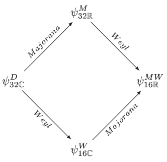
Figure A.1: Schematic view of how a ten-dimensional Dirac spinor can be projected down to a Majorana-Weyl spinor along two different routes. The number of real or complex degrees of freedom for each spinor is also indicated. The relation between the spinors at the intermediate stage (in nine dimensions) is given by (A.17).

Appendix B Supergravity and Reductions

B.1 11D Supergravity

B.1.1 11D Supersymmetry Transformations and Field Equations

The supersymmetry transformation rules of $N=1$ eleven-dimensional supergravity read

$$\delta{e}_{{\mu}}{}^{{a}} =\bar{{\epsilon}}{\Gamma}^{{a}}{\psi}_{{\mu}}\,,$$

$$\delta{{C}}_{{\mu}{\nu}{\rho}} =-3\,\bar{{{\epsilon}}}{\Gamma}_{[{\mu}{\nu}}{\psi}_{{\rho}]}\,,$$

$$\delta{\psi}_{{\mu}} =D_{{\mu}}{\epsilon}+\tfrac{1}{192}(\not{G}{\Gamma}_{{\mu}}-\tfrac{1}{3}{\Gamma}_{{\mu}}\not{G}){\epsilon}\,,$$ (B.1)

with the field strengths ${G}=\text{d}{C}$ and $D_{{\mu}}{\epsilon}=(\partial_{{\mu}}+{\omega}_{{\mu}}){\epsilon}$. The 11D fermionic field content consists solely of a 32–component gravitino, whose field equation reads

$$X_{0}({{\psi}}^{{{\mu}}})={{\Gamma}}^{{{\mu}}{{\nu}}{{\rho}}}{{D}}_{{{\nu}}}{{\psi}}_{{{\rho}}}=0\,,$$ (B.2)

with ${{D}}_{{{\nu}}}=\partial_{{{\nu}}}+{{\omega}}_{{{\nu}}}$ and where we have set the three-form equal to zero. Under supersymmetry this fermionic field equations transforms into

$$\delta_{0}X_{0}({{\psi}}^{{{\mu}}})=\tfrac{1}{2}{{\Gamma}}^{{{\nu}}}{{\epsilon}}\,[{{R}}^{{{\mu}}}{}_{{{\nu}}}-\tfrac{1}{2}{{R}}{{g}}^{{{\mu}}}{}_{{{\nu}}}]\,,$$ (B.3)

which implies the bosonic Einstein equation for the metric.

B.1.2 11D Reduction Ansätze to IIA

We use the following reduction Ansätze (where hatted quantities are 11D and unhatted are IIA)

$${{\hat{e}}}_{{\hat{\mu}}}{}^{{\hat{a}}} =e^{m_{11}z}\left(\begin{array}[]{cc}e^{-\phi/12}e_{\mu}{}^{a}&-e^{2\phi/3}C^{(1)}_{\mu}\\ 0&e^{2\phi/3}\end{array}\right)\,,$$ (B.5)

$${\hat{\psi}}_{a} =e^{-m_{11}z/2}e^{\phi/24}[\psi_{a}-\tfrac{1}{24}\Gamma_{a}\lambda]\,,$$

$${\hat{\psi}}_{\underline{z}} =\tfrac{1}{3}e^{-m_{11}z/2}e^{\phi/24}\Gamma_{\underline{z}}\lambda\,,$$

$${\hat{\epsilon}} =e^{m_{11}z/2}e^{-\phi/24}\epsilon\,,$$

$${{\hat{C}}}_{\mu\nu\rho} =e^{3m_{11}z}C^{(3)}_{\mu\nu\rho}\,,$$

$${\hat{C}}_{\mu\nu z} =-e^{3m_{11}z}B_{\mu\nu}\,,$$ (B.6)

to arrive at the IIA supersymmetry transformations in ten dimensions, where

• $m_{11}=0$ for toroidal reduction and

• $m_{11}\neq 0$ for twisted reduction using the trombone symmetry of 11D supergravity.

B.2 IIA Supergravity

B.2.1 IIA Supersymmetry Transformations and Field Equations

The supersymmetry transformation rules of ten-dimensional massless or ungauged IIA supergravity read

$$\delta_{0}e_{\mu}{}^{a} =\overline{\epsilon}\Gamma^{a}{\psi}_{\mu}\,,$$

$$\delta_{0}{\psi}_{\mu} =\big{(}D_{\mu}+\tfrac{1}{48}e^{-\phi/2}(\not{H}{\Gamma}_{\mu}+\tfrac{1}{2}{\Gamma}_{\mu}\not{H})\Gamma_{\text{11}}+\tfrac{1}{16}e^{3\phi/4}(\not{G}^{(2)}{\Gamma}_{\mu}-\tfrac{3}{4}{\Gamma}_{\mu}\not{G}^{(2)})\Gamma_{\text{11}}+$$

$$\;\;\;+\tfrac{1}{192}e^{\phi/4}(\not{G}^{(4)}{\Gamma}_{\mu}-\tfrac{1}{4}{\Gamma}_{\mu}\not{G}^{(4)})\big{)}\epsilon\,,$$

$$\delta_{0}{B}_{\mu\nu} =2e^{\phi/2}\overline{\epsilon}\Gamma_{\text{11}}{\Gamma}_{[\mu}({\psi}_{\nu]}+\tfrac{1}{8}{\Gamma}_{\nu]}\lambda)\,,$$

$$\delta_{0}C^{(1)}_{\mu} =-e^{-3\phi/4}\overline{\epsilon}\Gamma_{\text{11}}({\psi}_{\mu}-\tfrac{3}{8}{\Gamma}_{\mu}\lambda)\,,$$

$$\delta_{0}C^{(3)}_{\mu\nu\rho} =-3e^{-\phi/4}\overline{\epsilon}{\Gamma}_{[\mu\nu}({\psi}_{\rho]}-\tfrac{1}{24}{\Gamma}_{\rho]}\lambda)+3C^{(1)}_{[\mu}\delta_{0}{B}_{\nu\rho]}\,,$$

$$\delta_{0}\lambda =\big{(}\not{\partial}\phi+\tfrac{1}{12}e^{-\phi/2}\not{H}\Gamma_{\text{11}}+\tfrac{3}{8}e^{3\phi/4}\not{G}^{(2)}\Gamma_{\text{11}}+\tfrac{1}{96}e^{\phi/4}\not{G}^{(4)}\big{)}\epsilon\,,$$

$$\delta_{0}\phi =\tfrac{1}{2}\overline{\epsilon}\lambda\,,$$ (B.7)

with the following field strengths:

$${G^{(2)}} ={\rm d}{C^{(1)}}\,,\qquad{H}={\rm d}{B}\,,\qquad{G^{(4)}}={\rm d}{C^{(3)}}+{C^{(1)}}{\scriptstyle\wedge}{H}\,,$$ (B.8)

and $D_{{\mu}}{\epsilon}=(\partial_{{\mu}}+{\omega}_{{\mu}}){\epsilon}$. Upon (massless) reduction with our Ansätze the 11D field equation splits up in two field equations for the 10D IIA fermionic field content, a gravitino and a dilatino:

$$X_{0}({{\psi}}^{{{\mu}}}) ={{\Gamma}}^{{{\mu}}{{\nu}}{{\rho}}}{{D}}_{{{\nu}}}{{\psi}}_{{{\rho}}}-\tfrac{1}{8}(\not{\partial}{\phi}){{\Gamma}}^{{{\mu}}}{\lambda}=0\,,\qquad X_{0}({\lambda})={{\Gamma}}^{{{\nu}}}{{D}}_{{{\nu}}}{\lambda}-{{\Gamma}}^{{{\nu}}}(\not{\partial}{\phi}){{\psi}}_{{{\nu}}}=0\,,$$ (B.9)

with ${{D}}_{{{\nu}}}=(\partial_{{{\nu}}}+{{\omega}}_{{{\nu}}})$ and where we have set the vector, two- and three-form equal to zero. Under supersymmetry these fermionic field equations transform into

$$\delta_{0}X_{0}({{\psi}}^{{{\mu}}})= \tfrac{1}{2}{{\Gamma}}^{{{\nu}}}{{\epsilon}}\,[{{R}}^{{{\mu}}}{}_{{{\nu}}}-\tfrac{1}{2}{{R}}{{g}}^{{{\mu}}}{}_{{{\nu}}}-\tfrac{1}{2}(\partial^{{{\mu}}}{\phi})(\partial_{{{\nu}}}{\phi})+\tfrac{1}{4}(\partial{\phi})^{2}{{g}}^{{{\mu}}}{}_{{{\nu}}}]\,,$$

$$\delta_{0}X_{0}({\lambda})= {\epsilon}\,[\Box{\phi}]\,,$$ (B.10)

which imply the usual graviton-dilaton field equations.

B.2.2 IIA Reduction Ansätze to 9D

We use the following reduction Ansatz with $z$-dependence implied by the $SO(1,1)$-symmetries (where hatted quantities are IIA and unhatted are 9D):

$${\hat{e}}_{\hat{\mu}}{}^{\hat{a}} =e^{9m_{\text{IIA}}z/8}\left(\begin{array}[]{cc}e^{\phi/16-3\varphi/16\sqrt{7}}e_{\mu}{}^{a}&e^{-7\phi/16+3\sqrt{7}\varphi/16}A_{\mu}^{1}\\ 0&e^{-7\phi/16+3\sqrt{7}\varphi/16}\end{array}\right)\,,$$ (B.13)

$${\hat{\psi}}_{a} =e^{-9m_{\text{IIA}}z/16}e^{-\phi/32+3\varphi/32\sqrt{7}}[\psi_{a}+\tfrac{1}{32}\Gamma_{a}(\lambda-\tfrac{3}{\sqrt{7}}{\tilde{\lambda}})]\,,$$

$${\hat{\psi}}_{\underline{z}} =-\tfrac{7}{32}e^{-9m_{\text{IIA}}z/16}e^{-\phi/32+3\varphi/32\sqrt{7}}\Gamma_{\underline{z}}(\lambda-\tfrac{3}{\sqrt{7}}\tilde{\lambda})\,,$$

$${\hat{B}}_{\mu\nu} =-e^{3m_{\text{IIA}}z+m_{4}z/2}(B_{\mu\nu}^{1}-2A^{1}_{[\mu}A_{\nu]})\,,$$

$${\hat{B}}_{\mu z} =-e^{3m_{\text{IIA}}z+m_{4}z/2}A_{\mu}\,,$$

$${\hat{C}}^{(1)}_{\mu} =-e^{-3m_{4}z/4}(A_{\mu}^{2}+\chi A^{1}_{\mu})\,,$$

$${\hat{C}}^{(1)}_{z} =-e^{-3m_{4}z/4}\chi\,,$$

$${\hat{C}}^{(3)}_{\mu\nu\rho} =e^{3m_{\text{IIA}}z-m_{4}z/4}(C_{\mu\nu\rho}-3A_{i\,[\mu}B^{i}_{\nu\rho]}+6A^{1}_{[\mu}A^{2}_{\nu}A_{\rho]})\,,$$

$${\hat{C}}^{(3)}_{\mu\nu z} =-e^{3m_{\text{IIA}}z-m_{4}z/4}(B_{\mu\nu}^{2}-2A^{2}_{[\mu}A_{\nu]})\,,$$

$${\hat{\lambda}} =\tfrac{1}{4}e^{-9m_{\text{IIA}}z/16}e^{-\phi/32+3\varphi/32\sqrt{7}}(3\lambda+\sqrt{7}\tilde{\lambda})\,,$$

$$\hat{\epsilon} =e^{9m_{\text{IIA}}z/16}e^{\phi/32-3\varphi/32\sqrt{7}}\epsilon\,,$$

$$\hat{\phi} =\tfrac{1}{4}(3\phi+\sqrt{7}\varphi)+\left(\tfrac{3}{2}m_{\text{IIA}}+m_{4}\right)z\,,$$ (B.14)

where the mass parameters are given by

• $m_{\text{IIA}}=0$ and $m_{4}=0$ for toroidal reduction,

• $m_{\text{IIA}}=0$ and $m_{4}\neq 0$ for twisted reduction using the scale symmetry $\alpha$,

• $m_{\text{IIA}}=0$ and $m_{4}\neq 0$ for twisted reduction using the trombone symmetry $\beta$ and

• $m_{\text{IIA}}\neq 0$ and $m_{4}\neq 0$ for a combination of the latter two.

B.3 IIB Supergravity

B.3.1 IIB Supersymmetry Transformations and Field Equations

The supersymmetry transformation rules of ten-dimensional IIB supergravity read (in complex notation)

$$\delta{e}_{\mu}\,^{a} =\tfrac{1}{2}{\overline{\epsilon}}\,{\Gamma}^{a}{\psi}_{\mu}+\text{h.c.}\,,$$

$$\delta\psi_{\mu} =D_{\mu}\epsilon-\tfrac{i}{16\cdot 5!}\not{G}^{\text{(5)}}{\Gamma}_{\mu}\epsilon\,$$

$$\quad+\tfrac{i}{16\cdot 3!}e^{\phi/2}\left({\Gamma}_{\mu}{\Gamma}^{(3)}+2{\Gamma}^{(3)}{\Gamma}_{\mu}\right)\left({H}^{2}+\tau{H}^{1}\right)_{(3)}{\epsilon}^{*}\,,$$

$$\delta\lambda =-e^{\phi}\not{\partial}\tau{\epsilon}^{*}-\tfrac{1}{2\cdot 3!}e^{\phi/2}{\Gamma}^{(3)}\left({H}^{2}+\tau{H}^{1}\right)_{(3)}\epsilon\,,$$

$$\delta{B}^{1}_{\mu\nu} =e^{\phi/2}\left({{\overline{\epsilon}}}^{*}\,{\Gamma}_{[\mu}{\psi}_{\nu]}-\tfrac{i}{8}{\overline{\epsilon}}\,{\Gamma}_{\mu\nu}\lambda\right)+\text{h.c.}\,,$$

$$\delta{B}^{2}_{\mu\nu} =-e^{\phi/2}{\tau}^{*}\left({\overline{\epsilon}}^{*}{\Gamma}_{[\mu}{\psi}_{\nu]}-\tfrac{i}{8}{\overline{\epsilon}}\,{\Gamma}_{\mu\nu}\lambda\right)+\text{h.c.}\,,$$

$$\delta C^{(4)}_{\mu\nu\lambda\rho} =2i\,{\overline{\epsilon}}\,{\Gamma}_{[\mu\nu\lambda}{\psi}_{\rho]}-\tfrac{3}{2}\,{B}_{i\,[\mu\nu}\delta{B}^{i}_{\lambda\rho]}+\text{h.c.}\,,$$

$$\delta\chi =-\tfrac{1}{4}e^{-\phi}{\overline{\epsilon}}{\lambda}^{*}+\text{h.c.}\,,$$

$$\delta\phi =\tfrac{i}{4}{\overline{\epsilon}}{\lambda}^{*}+\text{h.c.}\,,$$ (B.15)

with the complex scalar $\tau=\chi+ie^{-\phi}$, the axion $\chi=C^{(0)}$, the doublet $B^{i}=(-B,C^{(2)})$ and the field strengths

$$H^{i} ={\rm d}B^{i}\,,\qquad G^{(5)}={\rm d}C^{(4)}+\tfrac{1}{2}B_{i}{\scriptstyle\wedge}H^{i}\,.$$ (B.16)

Indices $i,j$ of $SL(2,\mathbb{R})$ are contracted with $\varepsilon_{ij}=-\varepsilon^{ij}$ with $\varepsilon_{12}=-\varepsilon_{21}=1$. The covariant derivative of the IIB Killing spinor reads

$$D_{\mu}\epsilon =(\partial_{\mu}+{\omega}_{\mu}+\tfrac{i}{4}e^{\phi}\partial_{\mu}\chi)\epsilon\,.$$ (B.17)

When truncating to the metric, scalars and fermions, the massless 9D fermionic field equations read

$$X_{0}({\psi}^{\mu}) ={\Gamma}^{{\mu}{\nu}{\rho}}(\partial_{\nu}+{{\omega}}_{{{{\nu}}}}+\tfrac{1}{4}ie^{{\phi}}\partial_{\nu}{\chi}){\psi}_{\rho}+\tfrac{1}{8}e^{\phi}(\not{\partial}{\tau}){\Gamma}^{\mu}{\lambda}^{*}=0\,,$$

$$X_{0}({\lambda}) ={\Gamma}^{\mu}(\partial_{\mu}+{{\omega}}_{{{{\mu}}}}+\tfrac{3}{4}ie^{{\phi}}\partial_{\mu}{\chi}){\lambda}+e^{\phi}{\Gamma}^{\mu}(\not{\partial}{\tau}){\psi}_{\mu}^{*}=0\,.$$ (B.18)

B.3.2 IIB Reduction Ansätze to 9D

The reduction Ansätze we used for reducing the above rules are (where hatted quantities are IIB and unhatted are 9D)

$$\hat{e}_{\hat{\mu}}\,^{\hat{a}} =e^{m_{\text{IIB}}z}\left(\begin{array}[]{cc}e^{\sqrt{7}\varphi/28}e_{\mu}\,^{a}&-e^{-\sqrt{7}\varphi/4}A_{\mu}\\ 0&e^{-\sqrt{7}\varphi/4}\end{array}\right)\,,$$ (B.21)

$$\hat{\psi}_{a} =e^{-m_{\text{IIB}}z/2}e^{-\sqrt{7}\varphi/56}\left(\frac{c\tau^{*}+d}{c\tau+d}\right)^{1/4}(\psi_{a}+\tfrac{1}{8\sqrt{7}}\Gamma_{a}\tilde{\lambda}^{*})\,,$$

$$\hat{\psi}_{\underline{z}} =-\tfrac{\sqrt{7}}{8}e^{-m_{\text{IIB}}z/2}e^{-\sqrt{7}\varphi/56}\left(\frac{c\tau^{*}+d}{c\tau+d}\right)^{1/4}\Gamma_{\underline{z}}\tilde{\lambda}^{*}\,,$$

$$\hat{\lambda} =ie^{-m_{\text{IIB}}z/2}e^{-\sqrt{7}\varphi/56}\left(\frac{c\tau^{*}+d}{c\tau+d}\right)^{3/4}\lambda\,,$$

$$\hat{\epsilon} =e^{m_{\text{IIB}}z/2}e^{\sqrt{7}\varphi/56}\left(\frac{c\tau^{*}+d}{c\tau+d}\right)^{1/4}\epsilon\,,$$

$$\hat{\tau} =\frac{a\tau+b}{c\tau+d}\,,$$

$$\hat{B}^{i}_{\mu\nu} =e^{2m_{\text{IIB}}z}(\Omega(z)^{-1})_{j}{}^{i}\,B^{j}_{\mu\nu}\,,\hskip 28.45274pt\hat{B}^{i}_{\mu z}=-e^{2m_{\text{IIB}}z}(\Omega(z)^{-1})_{j}{}^{i}\,A^{j}_{\mu}\,,$$

$$\hat{C}^{(4)}_{\mu\nu\lambda\rho} =e^{4m_{\text{IIB}}z}D_{\mu\nu\lambda\rho}\,,\hskip 42.67912pt\hat{C}^{(4)}_{\mu\nu\lambda z}=e^{4m_{\text{IIB}}z}(-C_{\mu\nu\lambda}+\tfrac{3}{2}A_{i\,[\mu}B^{i}_{\nu\rho]})\,,$$ (B.22)

where we take the $\Omega$ to be $z$-dependent:

$$\Omega(z)_{i}{}^{j} =\text{exp}\left(\begin{array}[]{cc}\tfrac{1}{2}m_{1}z&\tfrac{1}{2}(m_{2}+m_{3})z\\ \tfrac{1}{2}(m_{2}-m_{3})z&-\tfrac{1}{2}m_{1}z\end{array}\right)\,,$$ (B.25)

$$=\left(\begin{array}[]{cc}\cosh(\alpha z)+\tfrac{m_{1}}{2\alpha}\sinh(\alpha z)&\tfrac{1}{2\alpha}(m_{2}+m_{3})\sinh(\alpha z)\\ \tfrac{1}{2\alpha}(m_{2}-m_{3})\sinh(\alpha z)&\cosh(\alpha z)-\tfrac{m_{1}}{2\alpha}\sinh(\alpha z)\end{array}\right)\,,$$ (B.28)

where $\alpha^{2}=\tfrac{1}{4}(m_{1}{}^{2}+m_{2}{}^{2}-m_{3}{}^{2})$. The mass parameters $\vec{m}=(m_{1},m_{2},m_{3})$ and $m_{\text{IIB}}$ take the following values in the different reduction schemes

• $\vec{m}=0$ and $m_{\text{IIB}}=0$ for toroidal reduction,

• $\vec{m}\neq$ and $m_{\text{IIB}}=0$ for twisted reduction with the $SL(2,\mathbb{R})$ symmetry,

• $\vec{m}=0$ and $m_{\text{IIB}}\neq 0$ for twisted reduction with the trombone symmetry and

• $\vec{m}\neq 0$ and $m_{\text{IIB}}\neq 0$ for a combination of the latter two.

B.4 9D Maximal Supergravity

B.4.1 9D Supersymmetry Transformations and Field Equations

The unique nine-dimensional $N=2$ supergravity theory has the following supersymmetry transformations:

$$\delta_{0}e_{\mu}\,^{a} =\tfrac{1}{2}\bar{\epsilon}\gamma^{a}\psi_{\mu}+\text{h.c.}\,,$$

$$\delta_{0}\psi_{\mu} =D_{\mu}\epsilon+\tfrac{i}{16}e^{-2\varphi/\sqrt{7}}\left(\tfrac{5}{7}\gamma_{\mu}\gamma^{(2)}-\gamma^{(2)}\gamma_{\mu}\right)F_{(2)}\epsilon$$

$$\quad-\tfrac{1}{8\cdot 2!}e^{3\varphi/{2\sqrt{7}}}\left(\tfrac{5}{7}\gamma_{\mu}\gamma^{(2)}-\gamma^{(2)}\gamma_{\mu}\right)\,e^{\phi/2}\left(F^{2}+\tau F^{1}\right)_{(2)}\epsilon^{*}$$

$$\quad+\tfrac{i}{8\cdot 3!}e^{-\varphi/{2\sqrt{7}}}\left(\tfrac{3}{7}\gamma_{\mu}\gamma^{(3)}+\gamma^{(3)}\gamma_{\mu}\right)e^{\phi/2}\left(H^{2}+\tau H^{1}\right)_{(3)}\epsilon^{*}$$

$$\quad-\tfrac{1}{8\cdot 4!}e^{\varphi/\sqrt{7}}\left(\tfrac{1}{7}\gamma_{\mu}\gamma^{(4)}-\gamma^{(4)}\gamma_{\mu}\right)G_{(4)}\epsilon\,,$$

$$\delta_{0}\tilde{\lambda} =i\not{\partial}\varphi\,\epsilon^{*}-\tfrac{1}{\sqrt{7}}e^{-2\varphi/\sqrt{7}}\not{F}\epsilon^{*}-\tfrac{3i}{2\cdot 2!\sqrt{7}}e^{3\varphi/{2\sqrt{7}}}e^{\phi/2}\gamma^{(2)}\left(F^{2}+\tau^{*}F^{1}\right)_{(2)}\epsilon$$

$$\quad+\tfrac{1}{2\cdot 3!\sqrt{7}}e^{-\varphi/{2\sqrt{7}}}e^{\phi/2}\gamma^{(3)}\left(H^{2}+\tau^{*}H^{1}\right)_{(3)}\epsilon$$

$$\quad+\tfrac{i}{4!\sqrt{7}}e^{\varphi/\sqrt{7}}\not{G}\epsilon^{*}\,,$$

$$\delta_{0}\lambda =i\not{\partial}\phi\,\epsilon^{*}-e^{\phi}\not{\partial}\chi\,\epsilon^{*}-\tfrac{i}{2\cdot 2!}e^{3\sqrt{7}\varphi/14}e^{\phi/2}\gamma^{(2)}\left(F^{2}+\tau F^{1}\right)_{(2)}\epsilon$$

$$\quad-\tfrac{1}{2\cdot 3!}e^{-\sqrt{7}\varphi/14}e^{\phi/2}\gamma^{(3)}\left(H^{2}+\tau H^{1}\right)_{(3)}\epsilon\,,$$

$$\delta_{0}A_{\mu} =\tfrac{i}{2}e^{2\varphi/\sqrt{7}}\bar{\epsilon}(\psi_{\mu}-\tfrac{i}{\sqrt{7}}\gamma_{\mu}\tilde{\lambda}^{*})+\mbox{h.c.}\,,$$

$$\delta_{0}A^{1}_{\mu} =\tfrac{i}{2}e^{\phi/2}e^{-3\varphi/2\sqrt{7}}\left(\overline{\epsilon}^{*}\psi_{\mu}+\tfrac{i}{4}\overline{\epsilon}\gamma_{\mu}\lambda+\tfrac{3i}{4\sqrt{7}}\overline{\epsilon}^{*}\gamma_{\mu}{\tilde{\lambda}}^{*}\right)+\text{h.c.}\,,$$

$$\delta_{0}A^{2}_{\mu} =-\tfrac{i}{2}e^{\phi/2}\tau^{*}e^{-3\varphi/2\sqrt{7}}\left(\overline{\epsilon}^{*}\psi_{\mu}+\tfrac{i}{4}\overline{\epsilon}\gamma_{\mu}\lambda+\tfrac{3i}{4\sqrt{7}}\overline{\epsilon}^{*}\gamma_{\mu}{\tilde{\lambda}}^{*}\right)+\text{h.c.}\,,$$

$$\delta_{0}B^{1}_{\mu\nu} =-e^{\phi/2}e^{\varphi/2\sqrt{7}}\left(\overline{\epsilon}^{*}\gamma_{[\mu}\psi_{\nu]}+\tfrac{i}{8}{\overline{\epsilon}}\gamma_{\mu\nu}\lambda-\tfrac{i}{8\sqrt{7}}{\overline{\epsilon}}^{*}\gamma_{\mu\nu}{\tilde{\lambda}}^{*}\right)-A_{[\mu}^{\phantom{()}}\delta_{0}A^{1}_{\nu]}+\text{h.c.}\,,$$

$$\delta_{0}B^{2}_{\mu\nu} =e^{\phi/2}\tau^{*}e^{\varphi/2\sqrt{7}}\left(\overline{\epsilon}^{*}\gamma_{[\mu}\psi_{\nu]}+\tfrac{i}{8}{\overline{\epsilon}}\gamma_{\mu\nu}\lambda-\tfrac{i}{8\sqrt{7}}{\overline{\epsilon}}^{*}\gamma_{\mu\nu}{\tilde{\lambda}}^{*}\right)-A_{[\mu}^{\phantom{()}}\delta_{0}A^{2}_{\nu]}+\text{h.c.}\,,$$

$$\delta_{0}C_{\mu\nu\rho} =\tfrac{3}{2}e^{-\varphi/\sqrt{7}}\bar{\epsilon}\gamma_{[\mu\nu}\left(\psi_{\rho]}+\tfrac{i}{6\sqrt{7}}\gamma_{\rho]}\tilde{\lambda}^{*}\right)-\tfrac{3}{2}B_{i\,[\mu\nu}\,\delta_{0}A^{i}_{\rho]}+\mbox{h.c.}\,,$$

$$\delta_{0}\varphi =-\tfrac{i}{4}\bar{\epsilon}\tilde{\lambda}^{*}+\text{h.c.}\,,$$

$$\delta_{0}\chi =\tfrac{1}{4}e^{-\phi}\overline{\epsilon}\lambda^{*}+\text{h.c.}\,,$$

$$\delta_{0}\phi =-\tfrac{i}{4}\overline{\epsilon}\lambda^{*}+\text{h.c.}\,,$$ (B.29)

with the complex scalar $\tau=\chi+ie^{-\phi}$. The field strengths read

$$G^{(1)}={\rm d}\chi\,,\quad F={\rm d}A\,,\quad F^{i}={\rm d}A^{i}\,,\quad H^{i}={\rm d}B^{i}-A{\scriptstyle\wedge}F^{i}\,,\quad G={\rm d}C+B_{i}{\scriptstyle\wedge}F^{i}\,.$$ (B.30)

The covariant derivative of the Killing spinor reads

$$D_{\mu}\epsilon =(\partial_{\mu}+\omega_{\mu}+\tfrac{i}{4}e^{\phi}\partial_{\mu}\chi)\epsilon\,.$$ (B.31)

When truncating to the metric, scalars and fermions, the massless 9D fermionic field equations read

$$X_{0}(\psi^{\mu}) =\gamma^{\mu\nu\rho}(\partial_{\nu}+{{\omega}}_{{{\nu}}}+\tfrac{1}{4}ie^{\phi}\partial_{\nu}\chi)\psi_{\rho}-\tfrac{1}{8}e^{\phi}(\not{\partial}\tau)\gamma^{\mu}\lambda^{*}+\tfrac{1}{8}i(\not{\partial}\varphi)\gamma^{\mu}\tilde{\lambda}^{*}=0\,,$$

$$X_{0}(\lambda) =\gamma^{\mu}(\partial_{\mu}+{{\omega}}_{{{\mu}}}+\tfrac{3}{4}ie^{\phi}\partial_{\mu}\chi)\lambda+e^{\phi}\gamma^{\mu}(\not{\partial}\tau)\psi_{\mu}^{*}=0\,,$$

$$X_{0}(\tilde{\lambda}) =\gamma^{\mu}(\partial_{\mu}+{{\omega}}_{{{\mu}}}-\tfrac{1}{4}ie^{\phi}\partial_{\mu}\chi)\tilde{\lambda}-i\gamma^{\mu}(\not{\partial}\varphi)\psi_{\mu}^{*}=0\,.$$ (B.32)

Under supersymmetry these yield the variation

$$\delta_{0}X_{0}(\psi^{\mu}) =\tfrac{1}{2}{{\gamma}}^{{{\nu}}}{{\epsilon}}\,[{{R}}^{{{\mu}}}{}_{{{\nu}}}-\tfrac{1}{2}{{R}}{{g}}^{{{\mu}}}{}_{{{\nu}}}-\tfrac{1}{2}((\partial^{{{\mu}}}{\phi})(\partial_{{{\nu}}}{\phi})-\tfrac{1}{2}(\partial{\phi})^{2}{{g}}^{{{\mu}}}{}_{{{\nu}}})+$$

$$\hskip 42.67912pt-\tfrac{1}{2}e^{2\phi}((\partial^{{{\mu}}}{\chi})(\partial_{{{\nu}}}{\chi})-\tfrac{1}{2}(\partial{\chi})^{2}{{g}}^{{{\mu}}}{}_{{{\nu}}})-\tfrac{1}{2}((\partial^{{{\mu}}}{\varphi})(\partial_{{{\nu}}}{\varphi})-\tfrac{1}{2}(\partial{\varphi})^{2}{{g}}^{{{\mu}}}{}_{{{\nu}}})]\,,$$

$$\delta_{0}X_{0}(\lambda) =\epsilon^{*}[-e^{\phi}(\Box\chi+2(\partial_{\mu}\phi)(\partial^{\mu}\chi))]+i\epsilon^{*}[\Box\phi-e^{2\phi}(\partial\chi)^{2}]\,,$$

$$\delta_{0}X_{0}(\tilde{\lambda}) =i\epsilon^{*}[\Box\varphi]\,,$$ (B.33)

which are the massless bosonic field equations for the metric and the scalars.

B.4.2 Twisted Reduction of IIA using $\beta$

The reduction of massless IIA supergravity using the scale symmetry $\beta$ of table 4.1 for twisting, with reduction Ansätze (B.14) with $m_{\text{IIA}}=0$, leads to a massive deformation with mass parameter $m_{4}$. Only the supersymmetry variations of the dilatini receive explicit massive deformations:

$$\delta_{m_{4}}\lambda=\tfrac{3}{4}m_{4}e^{\phi/2-3\varphi/2\sqrt{7}}\epsilon\,,\qquad\delta_{m_{4}}\tilde{\lambda}=\tfrac{\sqrt{7}}{4}m_{4}e^{\phi/2-3\varphi/2\sqrt{7}}\epsilon\,.$$ (B.34)

The implicit massive deformations read:

$${\rm D}\phi =e^{-\phi}{\rm D}e^{\phi}\,,\qquad{\rm D}\varphi=e^{-\varphi}{\rm D}e^{\varphi}\,,\qquad G^{(1)}={\rm D}\chi+\tfrac{3}{4}m_{4}A^{2}\,,\qquad G={\rm D}C+B_{i}{\scriptstyle\wedge}F^{i}\,,$$

$$F ={\rm D}A+\tfrac{1}{2}m_{4}B^{1}\,,\qquad F^{1}={\rm d}A^{1}\,,\qquad F^{2}={\rm D}A^{2}\,,$$

$$H^{1} ={\rm D}B^{1}-A{\scriptstyle\wedge}F^{1}\,,\qquad H^{2}={\rm D}B^{2}-A{\scriptstyle\wedge}F^{2}-\tfrac{1}{4}m_{4}(C+3A^{2}{\scriptstyle\wedge}B^{1})\,.$$ (B.35)

The $\mathbb{R}^{+}$ covariant derivative is defined by ${\rm D}={\rm d}-w_{\beta}\,m_{4}A^{1}$ with $w_{\beta}$ the $\beta$ scale weight of the field it acts on, as given in the table 4.2, and ${\rm DD}=-w_{\beta}\,m_{4}F^{1}$. The covariant derivative of the supersymmetry parameter has no massive deformation.

As for the field equations, the explicit deformations in the bosonic sector are given by the scalar potential

$$V=\tfrac{1}{2}e^{\phi-3\varphi/\sqrt{7}}m_{4}{}^{2}\,,$$ (B.36)

which can not be written in terms of a superpotential as (4.1). The explicit deformations of the fermionic field equations read

$$X_{m_{4}}(\psi^{\mu}) =im_{4}e^{\phi/2-3\varphi/2\sqrt{7}}\gamma^{\mu\nu}[-i\tfrac{3}{256}\gamma_{\nu}\lambda-i\tfrac{\sqrt{7}}{256}\gamma_{\nu}\tilde{\lambda}]\,,$$

$$X_{m_{4}}(\lambda) =-m_{4}e^{\phi/2-3\varphi/2\sqrt{7}}\gamma^{\nu}[\tfrac{3}{4}\psi_{\nu}+\tfrac{2}{9\sqrt{7}}i\gamma_{\nu}\tilde{\lambda}^{*}]\,,$$

$$X_{m_{4}}(\tilde{\lambda}) =-m_{4}e^{\phi/2-3\varphi/2\sqrt{7}}\gamma^{\nu}[\tfrac{\sqrt{7}}{4}\psi_{\nu}-\tfrac{2}{9\sqrt{7}}i\gamma_{\nu}\lambda^{*}]\,.$$ (B.37)

These massive deformations can be seen as a gauging of the scale symmetry $\beta$ with gauge field transformation

$$\qquad\Lambda=e^{-w_{\beta}m_{4}\lambda^{1}}\,,\qquad A^{1} \rightarrow A^{1}-{\rm d}\lambda^{1}\,,$$ (B.38)

with gauge vector $A^{1}$ and parameter $\lambda^{1}$. In addition, we find that the parabolic $\mathbb{R}$ subgroup of $SL(2,\mathbb{R})$ is gauged:

$$\chi\rightarrow\chi+\tfrac{3}{4}m_{4}\lambda^{2}\,,\quad B^{2}\rightarrow B^{2}-\tfrac{3}{4}m_{4}\lambda^{2}B^{1}\,,\quad A^{2}\rightarrow A^{2}-d\lambda^{2}-\tfrac{3}{4}m_{4}\lambda^{2}A^{1}\,,$$ (B.39)

with gauge vector $A^{2}$ and parameter $\lambda^{2}$. These two symmetries do not commute but rather form the two–dimensional non-Abelian Lie group, consisting of scalings and translations in one dimension (so-called collinear transformations [199]). The algebra reads

$$[T_{1},T_{2}]=T_{2}\,,$$ (B.40)

which is non–semi–simple. The emergence of this non-Abelian group is an example of the enhanced gaugings of subsection 3.3.4 and can be understood by the scaling of the 10D vector $A_{\mu}$ under $\beta$, see table 4.1.

B.4.3 Twisted Reduction of IIA using $\alpha$

The twisted reduction of massless IIA supergravity based on the $\alpha$ symmetry of table 4.1, with reduction Ansätze (B.14) with $m_{4}=0$, leads to a gauged supergravity with mass parameter $m_{\rm IIA}$. The explicit massive deformations in this case appear in the variation of the gravitino and one of the dilatini:

$$\delta_{m_{\text{IIA}}}\psi_{\mu}=-\tfrac{9}{14}im_{\text{IIA}}e^{\phi/2-3\varphi/2\sqrt{7}}\gamma_{\mu}\epsilon^{*}\,,\qquad\delta_{m_{\text{IIA}}}\tilde{\lambda}=\tfrac{6}{\sqrt{7}}m_{\text{IIA}}e^{\phi/2-3\varphi/2\sqrt{7}}\epsilon\,.$$ (B.41)

The implicit massive deformations are given by

$${\rm D}\phi =e^{-\phi}{\rm d}e^{\phi}\,,\qquad{\rm D}\varphi=e^{-\varphi}{\rm D}e^{\varphi}\,,\qquad G^{(1)}={\rm d}\chi\,,\qquad G={\rm D}C+B_{i}{\scriptstyle\wedge}F^{i}\,,$$

$$F ={\rm D}A+3m_{\text{IIA}}B^{1}\,,\qquad F^{1}={\rm d}A^{1}\,,\qquad F^{2}={\rm d}A^{2}\,,$$

$$H^{1} ={\rm D}B^{1}-A{\scriptstyle\wedge}F^{1}\,,\qquad H^{2}={\rm D}B^{2}-A{\scriptstyle\wedge}F^{2}+3m_{\text{IIA}}C\,.$$ (B.42)

The $\mathbb{R}^{+}$ covariant derivative is defined by ${\rm D}={\rm d}-w_{\alpha}\,m_{\text{IIA}}A^{1}$ with $w_{\alpha}$ the scale weight under $\alpha$ of the field it acts on, as given in the table 4.2, and ${\rm DD}=-w_{\alpha}\,m_{\text{IIA}}F^{1}$. The covariant derivative of the supersymmetry parameter is given by

$$D_{\mu}\epsilon =(\partial_{\mu}+{\omega}_{\mu}+\tfrac{i}{4}e^{\phi}\partial_{\mu}\chi-\tfrac{9}{14}m_{\text{IIA}}\Gamma_{\mu}\not{A}^{1})\epsilon\,.$$ (B.43)

The 9D fermionic field equations have the following explicit massive deformations:

$$X_{m_{\text{IIA}}}(\psi^{\mu}) =im_{\text{IIA}}e^{\phi/2-3\varphi/2\sqrt{7}}\gamma^{\mu\nu}[\tfrac{9}{2}\psi_{\nu}^{*}-i\tfrac{9}{32}\gamma_{\nu}\lambda+i\tfrac{3}{4\sqrt{7}}\gamma_{\nu}\tilde{\lambda}]\,,$$

$$X_{m_{\text{IIA}}}(\lambda) =-m_{\text{IIA}}e^{\phi/2-3\varphi/2\sqrt{7}}\gamma^{\nu}[-i\tfrac{\sqrt{7}}{6}\gamma_{\nu}\tilde{\lambda}^{*}]\,,$$

$$X_{m_{\text{IIA}}}(\tilde{\lambda}) =-m_{\text{IIA}}e^{\phi/2-3\varphi/2\sqrt{7}}\gamma^{\nu}[\tfrac{6}{\sqrt{7}}\psi_{\nu}-\tfrac{11}{6\sqrt{7}}i\gamma_{\nu}\lambda^{*}+\tfrac{1}{7}i\gamma_{\nu}\tilde{\lambda}^{*}]\,.$$ (B.44)

This massive deformation is a gauging of the scale symmetry $\alpha$ with transformation:

$$\Lambda=e^{-w_{\alpha}m_{\text{IIA}}\lambda^{1}}\,,\qquad A^{1}\rightarrow A^{1}-{\rm d}\lambda^{1}\,,$$ (B.45)

with gauge vector $A^{1}$ and parameter $\lambda^{1}$.

B.4.4 Twisted Reduction of IIB using $\delta$

The other possibility for twisted reduction of $D=10$ IIB supergravity involves the trombone symmetry of IIB supergravity. We use the reduction Ansätze given in (B.22) with $m_{1}=m_{2}=m_{3}=0$, yielding a massive deformation with parameter $m_{\text{IIB}}$. The explicit deformations of the supersymmetry rules read

$$\delta_{m_{\text{IIB}}}\psi_{\mu}=-\tfrac{4}{7}im_{\text{IIB}}e^{2\varphi/\sqrt{7}}\gamma_{\mu}\epsilon\,,\qquad\delta_{m_{\text{IIB}}}\tilde{\lambda}=-\tfrac{4}{\sqrt{7}}m_{\text{IIB}}e^{2\varphi/\sqrt{7}}\epsilon^{*}\,.$$ (B.46)

The implicit deformations read

$$F ={\rm d}A\,,\qquad{F}^{i}={\rm d}{A}^{i}-2m_{\text{IIB}}{B}^{i}\,,\qquad H^{i}={\rm d}B^{i}-A{\scriptstyle\wedge}F^{i}\,,$$

$$G ={\rm d}C+B_{i}{\scriptstyle\wedge}F^{i}+m_{\text{IIB}}B_{i}{\scriptstyle\wedge}B^{i}\,,\qquad D\varphi={\rm d}\varphi-\tfrac{4}{\sqrt{7}}m_{\text{IIB}}A\,,$$ (B.47)

for the bosons and

$$D_{\mu}\epsilon =(\partial_{\mu}+{\omega}_{\mu}+\tfrac{i}{4}e^{\phi}\partial_{\mu}\chi+\tfrac{4}{7}m_{\text{IIB}}\Gamma_{\mu}\not{A})\epsilon$$ (B.48)

for the supersymmetry parameter. The explicit deformations of the fermionic field equations read

$$X_{m_{\text{IIB}}}(\psi^{\mu}) =im_{\text{IIB}}e^{2\varphi/\sqrt{7}}\gamma^{\mu\nu}[4\psi_{\nu}-\tfrac{15}{16\sqrt{7}}i\gamma_{\nu}\tilde{\lambda}^{*}]\,,$$

$$X_{m_{\text{IIB}}}(\lambda) =m_{\text{IIB}}e^{2\varphi/\sqrt{7}}\gamma^{\nu}[\tfrac{4}{9}i\gamma_{\nu}\lambda]\,,$$

$$X_{m_{\text{IIB}}}(\tilde{\lambda}) =m_{\text{IIB}}e^{2\varphi/\sqrt{7}}\gamma^{\nu}[\tfrac{4}{\sqrt{7}}\psi_{\nu}^{*}-i\tfrac{4}{7}\gamma_{\nu}\tilde{\lambda}]\,.$$ (B.49)

This is a supergravity where the scale symmetry $\delta$ has been gauged, whose action reads

$$\Lambda=e^{w_{\delta}m_{\text{IIB}}\lambda}\,,\qquad A\rightarrow A-{\rm d}\lambda\,,\qquad{B}^{i}\rightarrow e^{2m_{\text{IIB}}\lambda}({B}^{i}-{A}^{i}\,{\rm d}\lambda)\,,$$ (B.50)

with gauge vector $A$ and parameter $\lambda$.

B.4.5 Toroidal Reduction of Gauged IIA

Finally, one can also consider the toroidal reduction of the $D=10$ IIA gauged supergravity of subsection 4.2.3, again with reduction Ansätze (B.14) with $m_{4}=m_{\text{IIA}}=0$. This leads to a $D=9$ gauged supergravity with the following explicit deformations

$$\delta_{m_{11}}{\psi}_{\mu}=\tfrac{9}{14}im_{11}e^{\phi/2-3\varphi/2\sqrt{7}}\tau\gamma_{\mu}\epsilon^{*}\,,\qquad\delta_{m_{11}}\tilde{\lambda}=-\tfrac{6}{\sqrt{7}}m_{11}e^{\phi/2-3\varphi/2\sqrt{7}}\tau^{*}\epsilon\,.$$ (B.51)

The bosonic implicit deformations read

$${\rm D}\varphi ={\rm d}\varphi-\tfrac{6}{\sqrt{7}}m_{11}A^{2}\,,\qquad F={\rm D}A+3m_{11}B^{2}\,,\qquad G={\rm D}C++B_{i}{\scriptstyle\wedge}F^{i}\,,$$

$$F^{i} =dA^{i}\,,\qquad H^{1}={\rm D}B^{1}-A{\scriptstyle\wedge}F^{(1)}-3m_{11}C\,,\qquad H^{2}={\rm D}B^{2}-A{\scriptstyle\wedge}F^{(2)}\,,$$ (B.52)

with the scale covariant derivative of a field with weight $w$ defined by ${\rm D}={\rm d}-w_{\alpha}m_{11}A^{2}$. For the supersymmetry parameter we find

$$D_{\mu}\epsilon =(\partial_{\mu}+{\omega}_{\mu}+\tfrac{i}{4}e^{\phi}\partial_{\mu}\chi+\tfrac{9}{14}m_{11}\Gamma_{\mu}\not{A}^{2})\epsilon\,.$$ (B.53)

The fermionic field equations are deformed by the massive contributions

$$X_{m_{11}}(\psi^{\mu}) =-im_{11}e^{\phi/2-3\varphi/2\sqrt{7}}\gamma^{\mu\nu}[\tfrac{9}{2}\tau\psi_{\nu}^{*}-i\tfrac{9}{32}\tau^{*}\gamma_{\nu}\lambda+i\tfrac{3}{4\sqrt{7}}\tau\gamma_{\nu}\tilde{\lambda}]\,,$$

$$X_{m_{11}}(\lambda) =m_{11}e^{\phi/2-3\varphi/2\sqrt{7}}\gamma^{\nu}[-i\tau\tfrac{\sqrt{7}}{6}\gamma_{\nu}\tilde{\lambda}^{*}]\,,$$

$$X_{m_{11}}(\tilde{\lambda}) =m_{11}e^{\phi/2-3\varphi/2\sqrt{7}}\gamma^{\nu}[\tfrac{6}{\sqrt{7}}\tau^{*}\psi_{\nu}-\tfrac{11}{6\sqrt{7}}i\tau\gamma_{\nu}\lambda^{*}+\tfrac{1}{7}i\tau^{*}\gamma_{\nu}\tilde{\lambda}^{*}]\,.$$ (B.54)

This massive deformation is a gauging of the scale symmetry $\alpha$, reading

$$\Lambda=e^{-w_{\alpha}m_{11}\lambda^{2}}\,,\qquad A^{2}\rightarrow A^{2}-{\rm d}\lambda^{2}\,,$$ (B.55)

with gauge vector $A^{2}$ and parameter $\lambda^{2}$.

References

- [1] M. B. Green, J. H. Schwarz and E. Witten, Superstring theory. Vol. 1: Introduction, Cambridge, Uk: Univ. Pr. ( 1987) 469 P. ( Cambridge Monographs On Mathematical Physics).
- [2] M. B. Green, J. H. Schwarz and E. Witten, Superstring theory. Vol. 2: Loop amplitedes, anomalies and phenomonology, Cambridge, Uk: Univ. Pr. ( 1987) 596 P. ( Cambridge Monographs On Mathematical Physics).
- [3] J. Polchinski, String theory. Vol. 1: An introduction to the bosonic string, Cambridge, UK: Univ. Pr. (1998) 402 p.
- [4] J. H. Schwarz, Lectures on superstring and M theory dualities, Nucl. Phys. Proc. Suppl. 55B (1997) 1–32 [hep-th/9607201].
- [5] A. Sen, An introduction to non-perturbative string theory, hep-th/9802051.
- [6] J. Polchinski, String theory. Vol. 2: Superstring theory and beyond, Cambridge, UK: Univ. Pr. (1998) 531 p.
- [7] J. Scherk and J. H. Schwarz, Dual models for nonhadrons, Nucl. Phys. B81 (1974) 118–144.
- [8] E. Witten, String theory dynamics in various dimensions, Nucl. Phys. B443 (1995) 85–126 [hep-th/9503124].
- [9] C. M. Hull and P. K. Townsend, Unity of superstring dualities, Nucl. Phys. B438 (1995) 109–137 [hep-th/9410167].
- [10] J. Dai, R. G. Leigh and J. Polchinski, New connections between string theories, Mod. Phys. Lett. A4 (1989) 2073–2083.
- [11] J. Polchinski, Dirichlet-Branes and Ramond-Ramond Charges, Phys. Rev. Lett. 75 (1995) 4724–4727 [hep-th/9510017].
- [12] A. Strominger and C. Vafa, Microscopic Origin of the Bekenstein-Hawking Entropy, Phys. Lett. B379 (1996) 99–104 [hep-th/9601029].
- [13] J. M. Maldacena, The large N limit of superconformal field theories and supergravity, Adv. Theor. Math. Phys. 2 (1998) 231–252 [hep-th/9711200].
- [14] N. Itzhaki, J. M. Maldacena, J. Sonnenschein and S. Yankielowicz, Supergravity and the large N limit of theories with sixteen supercharges, Phys. Rev. D58 (1998) 046004 [hep-th/9802042].
- [15] H. J. Boonstra, K. Skenderis and P. K. Townsend, The domain wall/QFT correspondence, JHEP 01 (1999) 003 [hep-th/9807137].
- [16] L. Randall and R. Sundrum, A large mass hierarchy from a small extra dimension, Phys. Rev. Lett. 83 (1999) 3370–3373 [hep-ph/9905221].
- [17] L. Randall and R. Sundrum, An alternative to compactification, Phys. Rev. Lett. 83 (1999) 4690–4693 [hep-th/9906064].
- [18] P. K. Townsend, Quintessence from M-theory, JHEP 11 (2001) 042 [hep-th/0110072].
- [19] R. Kallosh, A. D. Linde, S. Prokushkin and M. Shmakova, Gauged supergravities, de Sitter space and cosmology, Phys. Rev. D65 (2002) 105016 [hep-th/0110089].
- [20] J. Scherk and J. H. Schwarz, Spontaneous breaking of supersymmetry through dimensional reduction, Phys. Lett. B82 (1979) 60.
- [21] J. Scherk and J. H. Schwarz, How to get masses from extra dimensions, Nucl. Phys. B153 (1979) 61–88.
- [22] S. R. Coleman and J. Mandula, All possible symmetries of the S matrix, Phys. Rev. 159 (1967) 1251–1256.
- [23] R. Haag, J. T. Lopuszanski and M. Sohnius, All possible generators of supersymmetries of the S matrix, Nucl. Phys. B88 (1975) 257.
- [24] D. Z. Freedman, P. van Nieuwenhuizen and S. Ferrara, Progress toward a Theory of Supergravity, Phys. Rev. D13 (1976) 3214–3218.
- [25] A. Van Proeyen, Tools for supersymmetry, hep-th/9910030.
- [26] B. de Wit, Supergravity, hep-th/0212245.
- [27] W. Nahm, Supersymmetries and their representations, Nucl. Phys. B135 (1978) 149.
- [28] M. A. Vasiliev, Higher-spin gauge theories in four, three and two dimensions, Int. J. Mod. Phys. D5 (1996) 763–797 [hep-th/9611024].
- [29] P. K. Townsend, The eleven-dimensional supermembrane revisited, Phys. Lett. B350 (1995) 184–187 [hep-th/9501068].
- [30] J. H. Schwarz, The power of M theory, Phys. Lett. B367 (1996) 97–103 [hep-th/9510086].
- [31] E. Cremmer, B. Julia and J. Scherk, Supergravity theory in 11 dimensions, Phys. Lett. B76 (1978) 409–412.
- [32] E. Cremmer, H. Lu, C. N. Pope and K. S. Stelle, Spectrum-generating symmetries for BPS solitons, Nucl. Phys. B520 (1998) 132–156 [hep-th/9707207].
- [33] M. B. Green and J. H. Schwarz, Anomaly cancellation in supersymmetric D=10 gauge theory and superstring theory, Phys. Lett. B149 (1984) 117–122.
- [34] E. Bergshoeff, R. Kallosh, T. Ortin, D. Roest and A. Van Proeyen, New formulations of D = 10 supersymmetry and D8 - O8 domain walls, Class. Quant. Grav. 18 (2001) 3359–3382 [hep-th/0103233].
- [35] E. Bergshoeff, H. J. Boonstra and T. Ortin, S duality and dyonic p-brane solutions in type II string theory, Phys. Rev. D53 (1996) 7206–7212 [hep-th/9508091].
- [36] M. B. Green, C. M. Hull and P. K. Townsend, D-Brane Wess-Zumino Actions, T-Duality and the Cosmological Constant, Phys. Lett. B382 (1996) 65–72 [hep-th/9604119].
- [37] L. J. Romans, Massive N=2a supergravity in ten dimensions, Phys. Lett. B169 (1986) 374.
- [38] F. Giani and M. Pernici, N=2 supergravity in ten dimensions, Phys. Rev. D30 (1984) 325–333.
- [39] I. C. G. Campbell and P. C. West, N=2 D = 10 nonchiral supergravity and its spontaneous compactification, Nucl. Phys. B243 (1984) 112.
- [40] J. H. Schwarz, Covariant field equations of chiral N=2 D = 10 supergravity, Nucl. Phys. B226 (1983) 269.
- [41] P. S. Howe and P. C. West, The complete N=2, d = 10 supergravity, Nucl. Phys. B238 (1984) 181.
- [42] P. Pasti, D. P. Sorokin and M. Tonin, On Lorentz invariant actions for chiral p-forms, Phys. Rev. D55 (1997) 6292–6298 [hep-th/9611100].
- [43] J. H. Schwarz and P. C. West, Symmetries and transformations of chiral N=2 D = 10 supergravity, Phys. Lett. B126 (1983) 301.
- [44] S. Sethi and M. Stern, D-brane bound states redux, Commun. Math. Phys. 194 (1998) 675–705 [hep-th/9705046].
- [45] M. Dine, P. Y. Huet and N. Seiberg, Large and small radius in string theory, Nucl. Phys. B322 (1989) 301.
- [46] A. Giveon, M. Porrati and E. Rabinovici, Target space duality in string theory, Phys. Rept. 244 (1994) 77–202 [hep-th/9401139].
- [47] M. Abou-Zeid, B. de Wit, D. Lust and H. Nicolai, Space-time supersymmetry, IIA/B duality and M-theory, Phys. Lett. B466 (1999) 144–152 [hep-th/9908169].
- [48] C. Montonen and D. I. Olive, Magnetic monopoles as gauge particles?, Phys. Lett. B72 (1977) 117.
- [49] C. Pope, Kaluza-Klein Theory, lecture notes, see http://faculty.physics.tamu.edu/pope/ihplec.ps.
- [50] H. Lu and C. N. Pope, p-brane Solitons in Maximal Supergravities, Nucl. Phys. B465 (1996) 127–156 [hep-th/9512012].
- [51] E. Cremmer and B. Julia, The N=8 supergravity theory. 1. the Lagrangian, Phys. Lett. B80 (1978) 48.
- [52] B. Julia, Group disintegrations, Invited paper presented at Nuffield Gravity Workshop, Cambridge, Eng., Jun 22 - Jul 12, 1980.
- [53] E. Cremmer, Supergravities in 5 dimensions, Invited paper at the Nuffield Gravity Workshop, Cambridge, Eng., Jun 22 - Jul 12, 1980.
- [54] E. Cremmer, B. Julia, H. Lu and C. N. Pope, Dualisation of dualities. I, Nucl. Phys. B523 (1998) 73–144 [hep-th/9710119].
- [55] I. V. Lavrinenko, H. Lu, C. N. Pope and T. A. Tran, U-duality as general coordinate transformations, and spacetime geometry, Int. J. Mod. Phys. A14 (1999) 4915–4942 [hep-th/9807006].
- [56] M. J. Duff, R. R. Khuri and J. X. Lu, String solitons, Phys. Rept. 259 (1995) 213–326 [hep-th/9412184].
- [57] K. S. Stelle, BPS branes in supergravity, hep-th/9803116.
- [58] H. Lu, C. N. Pope, E. Sezgin and K. S. Stelle, Stainless super p-branes, Nucl. Phys. B456 (1995) 669–698 [hep-th/9508042].
- [59] G. W. Gibbons and P. K. Townsend, Vacuum interpolation in supergravity via super p-branes, Phys. Rev. Lett. 71 (1993) 3754–3757 [hep-th/9307049].
- [60] K. Behrndt, E. Bergshoeff, R. Halbersma and J. P. van der Schaar, On domain-wall/QFT dualities in various dimensions, Class. Quant. Grav. 16 (1999) 3517–3552 [hep-th/9907006].
- [61] G. T. Horowitz and A. Strominger, Black strings and P-branes, Nucl. Phys. B360 (1991) 197–209.
- [62] M. J. Duff and J. X. Lu, Black and super p-branes in diverse dimensions, Nucl. Phys. B416 (1994) 301–334 [hep-th/9306052].
- [63] B. R. Greene, A. D. Shapere, C. Vafa and S.-T. Yau, Stringy cosmic strings and noncompact Calabi-Yau manifolds, Nucl. Phys. B337 (1990) 1.
- [64] E. Bergshoeff and J. P. van der Schaar, On M-9-branes, Class. Quant. Grav. 16 (1999) 23–39 [hep-th/9806069].
- [65] E. Bergshoeff, E. Eyras, R. Halbersma, C. Hull, Y. Lozano and J.-P. van der Schaar, Spacetime-filling branes and strings with sixteen supercharges, Nucl. Phys. B564 (2000) 29–59 [hep-th/9812224].
- [66] J. Figueroa-O’Farrill and G. Papadopoulos, Maximally supersymmetric solutions of ten- and eleven- dimensional supergravities, JHEP 03 (2003) 048 [hep-th/0211089].
- [67] P. G. O. Freund and M. A. Rubin, Dynamics of dimensional reduction, Phys. Lett. B97 (1980) 233–235.
- [68] K. Pilch, P. van Nieuwenhuizen and P. K. Townsend, Compactification of d = 11 supergravity on S(4) (or 11 = 7 + 4, too), Nucl. Phys. B242 (1984) 377.
- [69] J. Kowalski-Glikman, Vacuum states in supersymmetric Kaluza-Klein theory, Phys. Lett. B134 (1984) 194–196.
- [70] M. Blau, J. Figueroa-O’Farrill, C. Hull and G. Papadopoulos, A new maximally supersymmetric background of IIB superstring theory, JHEP 01 (2002) 047 [hep-th/0110242].
- [71] M. Blau, J. Figueroa-O’Farrill, C. Hull and G. Papadopoulos, Penrose limits and maximal supersymmetry, Class. Quant. Grav. 19 (2002) L87–L95 [hep-th/0201081].
- [72] R. Penrose, Any space-time has a plane wave as a limit, Diff. Geom. and Rel., Reidel, Dordrecht (1976) 271–275.
- [73] R. Gueven, Plane wave limits and T-duality, Phys. Lett. B482 (2000) 255–263 [hep-th/0005061].
- [74] M. J. Duff and K. S. Stelle, Multi-membrane solutions of D = 11 supergravity, Phys. Lett. B253 (1991) 113–118.
- [75] R. Gueven, Black p-brane solutions of D = 11 supergravity theory, Phys. Lett. B276 (1992) 49–55.
- [76] A. Dabholkar, G. W. Gibbons, J. A. Harvey and F. Ruiz Ruiz, Superstrings and solitons, Nucl. Phys. B340 (1990) 33–55.
- [77] A. Strominger, Heterotic solitons, Nucl. Phys. B343 (1990) 167–184.
- [78] J. Polchinski and E. Witten, Evidence for Heterotic - Type I String Duality, Nucl. Phys. B460 (1996) 525–540 [hep-th/9510169].
- [79] C. M. Hull, Exact pp wave solutions of 11-dimensional supergravity, Phys. Lett. B139 (1984) 39.
- [80] M. Cvetic, H. Lu and C. N. Pope, M-theory pp-waves, Penrose limits and supernumerary supersymmetries, Nucl. Phys. B644 (2002) 65–84 [hep-th/0203229].
- [81] J. P. Gauntlett and C. M. Hull, pp-waves in 11-dimensions with extra supersymmetry, JHEP 06 (2002) 013 [hep-th/0203255].
- [82] I. Bena and R. Roiban, Supergravity pp-wave solutions with 28 and 24 supercharges, Phys. Rev. D67 (2003) 125014 [hep-th/0206195].
- [83] H. Brinkmann Proc. Nat. Acad. Sci. 9 (1923) 1.
- [84] D. J. Gross and M. J. Perry, Magnetic monopoles in Kaluza-Klein theories, Nucl. Phys. B226 (1983) 29.
- [85] R. D. Sorkin, Kaluza-Klein Monopole, Phys. Rev. Lett. 51 (1983) 87–90.
- [86] S. W. Hawking, Gravitational instantons, Phys. Lett. A60 (1977) 81.
- [87] G. Papadopoulos and P. K. Townsend, Intersecting M-branes, Phys. Lett. B380 (1996) 273–279 [hep-th/9603087].
- [88] J. P. Gauntlett, Intersecting branes, hep-th/9705011.
- [89] M. J. Duff, B. E. W. Nilsson and C. N. Pope, Kaluza-Klein supergravity, Phys. Rept. 130 (1986) 1–142.
- [90] T. Kaluza, On the problem of unity in physics, Sitzungsber. Preuss. Akad. Wiss. Berlin (Math. Phys. ) 1921 (1921) 966–972.
- [91] O. Klein, Quantum theory and five-dimensional theory of relativity, Z. Phys. 37 (1926) 895–906.
- [92] A. Dabholkar and C. Hull, Duality twists, orbifolds, and fluxes, JHEP 09 (2003) 054 [hep-th/0210209].
- [93] B. S. DeWitt in Relativity, groups and topology, Les Houches 1963 (Gordon and Breach, 1964).
- [94] Y. M. Cho and P. G. O. Freund, Nonabelian gauge fields in Nambu-Goldstone fields, Phys. Rev. D12 (1975) 1711.
- [95] M. Cvetic, H. Lu and C. N. Pope, Consistent Kaluza-Klein sphere reductions, Phys. Rev. D62 (2000) 064028 [hep-th/0003286].
- [96] H. Nastase, D. Vaman and P. van Nieuwenhuizen, Consistent nonlinear K K reduction of 11d supergravity on AdS(7) x S(4) and self-duality in odd dimensions, Phys. Lett. B469 (1999) 96–102 [hep-th/9905075].
- [97] H. Nastase, D. Vaman and P. van Nieuwenhuizen, Consistency of the AdS(7) x S(4) reduction and the origin of self-duality in odd dimensions, Nucl. Phys. B581 (2000) 179–239 [hep-th/9911238].
- [98] B. de Wit and H. Nicolai, The consistency of the S**7 truncation in d = 11 supergravity, Nucl. Phys. B281 (1987) 211.
- [99] M. Cvetic, H. Lu, C. N. Pope, A. Sadrzadeh and T. A. Tran, Consistent SO(6) reduction of type IIB supergravity on S(5), Nucl. Phys. B586 (2000) 275–286 [hep-th/0003103].
- [100] M. Cvetic, G. W. Gibbons, H. Lu and C. N. Pope, Consistent group and coset reductions of the bosonic string, Class. Quant. Grav. 20 (2003) 5161–5194 [hep-th/0306043].
- [101] M. J. Duff, B. E. W. Nilsson, N. P. Warner and C. N. Pope, Kaluza-Klein approach to the heterotic string. 2, Phys. Lett. B171 (1986) 170.
- [102] C. M. Hull and N. P. Warner, Noncompact gaugings from higher dimensions, Class. Quant. Grav. 5 (1988) 1517.
- [103] P. S. Howe, N. D. Lambert and P. C. West, A new massive type IIA supergravity from compactification, Phys. Lett. B416 (1998) 303–308 [hep-th/9707139].
- [104] I. V. Lavrinenko, H. Lu and C. N. Pope, Fibre bundles and generalised dimensional reductions, Class. Quant. Grav. 15 (1998) 2239–2256 [hep-th/9710243].
- [105] G. E. Sneddon, Hamiltonian Cosmology: a further investigation, J. Phys. Math. Gen. 9 (1976) 229.
- [106] J. M. Pons and P. Talavera, Consistent and inconsistent truncations: Some results and the issue of the correct uplifting of solutions, Nucl. Phys. B678 (2004) 427–454 [hep-th/0309079].
- [107] N. Alonso-Alberca, E. Bergshoeff, U. Gran, R. Linares, T. Ortín and D. Roest, Domain walls of D = 8 gauged supergravities and their D = 11 origin, JHEP 06 (2003) 038 [hep-th/0303113].
- [108] C. M. Hull and A. Catal-Ozer, Compactifications with S-duality twists, JHEP 10 (2003) 034 [hep-th/0308133].
- [109] M. Haack, J. Louis and H. Singh, Massive type IIA theory on K3, JHEP 04 (2001) 040 [hep-th/0102110].
- [110] B. Janssen, Massive T-duality in six dimensions, Nucl. Phys. B610 (2001) 280–292 [hep-th/0105016].
- [111] K. Behrndt, E. Bergshoeff, D. Roest and P. Sundell, Massive dualities in six dimensions, Class. Quant. Grav. 19 (2002) 2171–2200 [hep-th/0112071].
- [112] P. K. Townsend, Positive energy and the scalar potential in higher dimensional (super)gravity theories, Phys. Lett. B148 (1984) 55.
- [113] E. Bergshoeff, Y. Lozano and T. Ortin, Massive branes, Nucl. Phys. B518 (1998) 363–423 [hep-th/9712115].
- [114] C. M. Hull, Massive string theories from M-theory and F-theory, JHEP 11 (1998) 027 [hep-th/9811021].
- [115] P. West, The IIA, IIB and eleven dimensional theories and their common E(11) origin, hep-th/0402140.
- [116] E. Bergshoeff, T. de Wit, U. Gran, R. Linares and D. Roest, (Non-)Abelian gauged supergravities in nine dimensions, JHEP 10 (2002) 061 [hep-th/0209205].
- [117] E. Bergshoeff, M. de Roo, M. B. Green, G. Papadopoulos and P. K. Townsend, Duality of Type II 7-branes and 8-branes, Nucl. Phys. B470 (1996) 113–135 [[hep-th/9601150]].
- [118] P. Meessen and T. Ortín, An Sl(2,Z) multiplet of nine-dimensional type II supergravity theories, Nucl. Phys. B541 (1999) 195–245 [[hep-th/9806120]].
- [119] J. Gheerardyn and P. Meessen, Supersymmetry of massive D = 9 supergravity, Phys. Lett. B525 (2002) 322–330 [[hep-th/0111130]].
- [120] C. M. Hull, Gauged D = 9 supergravities and Scherk-Schwarz reduction, [hep-th/0203146].
- [121] E. Bergshoeff, U. Gran and D. Roest, Type IIB seven-brane solutions from nine-dimensional domain walls, Class. Quant. Grav. 19 (2002) 4207–4226 [[hep-th/0203202]].
- [122] O. DeWolfe, T. Hauer, A. Iqbal and B. Zwiebach, Uncovering the symmetries on (p,q) 7-branes: Beyond the Kodaira classification, Adv. Theor. Math. Phys. 3 (1999) 1785–1833 [hep-th/9812028].
- [123] O. DeWolfe, T. Hauer, A. Iqbal and B. Zwiebach, Uncovering infinite symmetries on (p,q) 7-branes: Kac-Moody algebras and beyond, Adv. Theor. Math. Phys. 3 (1999) 1835–1891 [hep-th/9812209].
- [124] E. Bergshoeff, U. Gran, R. Linares, M. Nielsen, T. Ortín and D. Roest, The Bianchi classification of maximal D = 8 gauged supergravities, Class. Quant. Grav. 20 (2003) 3997–4014 [hep-th/0306179].
- [125] W. Kundt, The spatially homogeneous cosmological models, Gen. Rel. Grav. 35 (2003) 491–498 Based on a seminar by Engelbert Schücking, notes taken by Wolfgang Kundt.
- [126] A. Krasinski, C. G. Behr, E. Schücking, F. B. Estabrook, H. D. Wahlquist, G. F. R. Ellis, R. Jantzen and W. Kundt, The Bianchi classification in the Schücking-Behr approach, Gen. Rel. Grav. 35 (2003) 487–490.
- [127] F. B. Estabrook, H. D. Wahlquist and C. G. Behr, Dyadic analysis of spatial homogeneous world models, J. Math. Phys. 9 (1968) 497.
- [128] G. F. R. Ellis and M. A. H. MacCallum, A Class of homogeneous cosmological models, Commun. Math. Phys. 12 (1969) 108–141.
- [129] M. A. H. MacCallum in On Einstein’s path, essays in honor of Engelbert Schücking (1999) 299–317 Ed. A. Harvey, Springer.
- [130] L. Bianchi, Sugli spazi a tre dimensioni che ammettono un gruppo continuo di movimenti, Tomo XI (1898) 267. For an English translation see: www34.homepage.villanova.edu/robert.jantzen/bianchi/bianchi.html.
- [131] J. Schirmer, Hamiltonian reduction of Bianchi cosmologies, Class. Quant. Grav. 12 (1995) 1099 [gr-qc/9408008].
- [132] R. M. Wald, General Relativity, Chicago, USA: Univ. Pr. (1984) 491p.
- [133] M. Hamermesh, Group Theory and its Application to Physical Problems, New York, USA: Dover Publ. (1989) 509p.
- [134] A. Ashtekar and J. Samuel, Bianchi cosmologies: The Role of spatial topology,.
- [135] A. Salam and E. Sezgin, D = 8 supergravity, Nucl. Phys. B258 (1985) 284.
- [136] W. P. Thurston, The geometry and topology of 3-manifolds. Princeton UP, 1979.
- [137] J. Barrow and H. Kodama, The Isotropy of Compact Universes, Class. Quant. Grav. 18 (2001) 1753–1766 [gr-qc/0012075].
- [138] E. Bergshoeff, A. Collinucci, U. Gran, M. Nielsen and D. Roest, Transient quintessence from group manifold reductions or how all roads lead to Rome, hep-th/0312102.
- [139] C. M. Hull, The Minimal Couplings and Scalar Potentials of the Gauged Supergravities, Class. Quant. Grav. 2 (1985) 343.
- [140] L. Andrianopoli, F. Cordaro, P. Fre’ and L. Gualtieri, Non-semisimple gaugings of D = 5 N = 8 supergravity and FDAs, Class. Quant. Grav. 18 (2001) 395–414 [hep-th/0009048].
- [141] C. M. Hull, New gauged N = 8, D = 4 supergravities, Class. Quant. Grav. 20 (2003) 5407–5424 [hep-th/0204156].
- [142] H. Nicolai and H. Samtleben, Compact and noncompact gauged maximal supergravities in three dimensions, JHEP 04 (2001) 022 [hep-th/0103032].
- [143] B. de Wit, H. Nicolai and H. Samtleben, Gauged supergravities in three dimensions: A panoramic overview, hep-th/0403014.
- [144] B. de Wit and H. Nicolai, N=8 supergravity, Nucl. Phys. B208 (1982) 323.
- [145] H. J. Kim, L. J. Romans and P. van Nieuwenhuizen, The mass spectrum of chiral N=2 d = 10 supergravity on S**5, Phys. Rev. D32 (1985) 389.
- [146] M. Cvetic, H. Lu, C. N. Pope, A. Sadrzadeh and T. A. Tran, S(3) and S(4) reductions of type IIA supergravity, Nucl. Phys. B590 (2000) 233–251 [hep-th/0005137].
- [147] C. M. Hull, Noncompact gaugings OF N=8 supergravity, Phys. Lett. B142 (1984) 39.
- [148] C. M. Hull, More gaugings of N=8 supergravity, Phys. Lett. B148 (1984) 297–300.
- [149] N. Alonso-Alberca and T. Ortin, Gauged / massive supergravities in diverse dimensions, Nucl. Phys. B651 (2003) 263–290 [hep-th/0210011].
- [150] P. K. Townsend, K. Pilch and P. van Nieuwenhuizen, Selfduality in odd dimensions, Phys. Lett. 136B (1984) 38.
- [151] N. Alonso-Alberca, P. Meessen and T. Ortin, An SL(3,Z) multiplet of 8-dimensional type II supergravity theories and the gauged supergravity inside, Nucl. Phys. B602 (2001) 329–345 [hep-th/0012032].
- [152] M. Cvetic, G. W. Gibbons and C. N. Pope, Ghost-free de Sitter supergravities as consistent reductions of string and M-theory, hep-th/0401151.
- [153] M. Pernici and E. Sezgin, Spontaneous compactification of seven-dimensional supergravity theories, Class. Quant. Grav. 2 (1985) 673.
- [154] L. Andrianopoli, R. D’Auria, S. Ferrara and M. A. Lledo, Gauging of flat groups in four dimensional supergravity, JHEP 07 (2002) 010 [hep-th/0203206].
- [155] B. de Wit, H. Samtleben and M. Trigiante, On Lagrangians and gaugings of maximal supergravities, Nucl. Phys. B655 (2003) 93–126 [hep-th/0212239].
- [156] R. D’Auria, S. Ferrara, F. Gargiulo, M. Trigiante and S. Vaula, N = 4 supergravity Lagrangian for type IIB on T**6/Z(2) in presence of fluxes and D3-branes, JHEP 06 (2003) 045 [hep-th/0303049].
- [157] C. Angelantonj, S. Ferrara and M. Trigiante, New D = 4 gauged supergravities from N = 4 orientifolds with fluxes, JHEP 10 (2003) 015 [hep-th/0306185].
- [158] B. de Wit, H. Samtleben and M. Trigiante, Maximal supergravity from IIB flux compactifications, Phys. Lett. B583 (2004) 338–346 [hep-th/0311224].
- [159] A. Chamblin, M. J. Perry and H. S. Reall, Non-BPS D8-branes and dynamic domain walls in massive IIA supergravities, JHEP 09 (1999) 014 [hep-th/9908047].
- [160] A. Dabholkar, Lectures on orientifolds and duality, hep-th/9804208.
- [161] P. Horava and E. Witten, Heterotic and type I string dynamics from eleven dimensions, Nucl. Phys. B460 (1996) 506–524 [hep-th/9510209].
- [162] M. Cvetic, H. Lu and C. N. Pope, Consistent sphere reductions and universality of the Coulomb branch in the domain-wall / QFT correspondence, Nucl. Phys. B590 (2000) 213–232 [hep-th/0004201].
- [163] E. Bergshoeff, M. Nielsen and D. Roest, The domain walls of gauged maximal supergravities and their M-theory origin, hep-th/0404100.
- [164] H. Nicolai and H. Samtleben, A U(1) x SO(9) invariant compactification of D = 11 supergravity to two dimensions, Prepared for 4th Annual European TMR Conference on Integrability Nonperturbative Effects and Symmetry in Quantum Field Theory, Paris, France, 7-13 Sep 2000.
- [165] T. Fischbacher, H. Nicolai and H. Samtleben, Non-semisimple and complex gaugings of N = 16 supergravity, hep-th/0306276.
- [166] I. Bakas, A. Brandhuber and K. Sfetsos, Domain walls of gauged supergravity, M-branes, and algebraic curves, Adv. Theor. Math. Phys. 3 (1999) 1657 [hep-th/9912132].
- [167] M. Cvetic, S. S. Gubser, H. Lu and C. N. Pope, Symmetric potentials of gauged supergravities in diverse dimensions and Coulomb branch of gauge theories, Phys. Rev. D62 (2000) 086003 [hep-th/9909121].
- [168] I. Bakas and K. Sfetsos, States and curves of five-dimensional gauged supergravity, Nucl. Phys. B573 (2000) 768–810 [hep-th/9909041].
- [169] I. Bakas and K. Sfetsos, Gravitational domain walls and p-brane distributions, Fortsch. Phys. 49 (2001) 419–431 [hep-th/0012125].
- [170] J. G. Russo, New compactifications of supergravities and large N QCD, Nucl. Phys. B543 (1999) 183–197 [hep-th/9808117].
- [171] P. Kraus, F. Larsen and S. P. Trivedi, The Coulomb branch of gauge theory from rotating branes, JHEP 03 (1999) 003 [hep-th/9811120].
- [172] P. M. Cowdall, Novel domain wall and Minkowski vacua of D = 9 maximal SO(2) gauged supergravity, Nucl. Phys. B600 (2001) 81 [hep-th/0009016].
- [173] H. Nishino and S. Rajpoot, Gauged N = 2 supergravity in nine-dimensions and domain wall solutions, [hep-th/0207246].
- [174] S. Chaudhuri, Confinement and the short type I’ flux tube, Nucl. Phys. B591 (2000) 243–264 [hep-th/0007056].
- [175] J. Kerimo, J. T. Liu, H. Lu and C. N. Pope, Supergravities with Minkowski x sphere vacua, hep-th/0402223.
- [176] A. Paredes, Supersymmetric solutions of supergravity from wrapped branes, hep-th/0407013.
- [177] P. M. Cowdall, H. Lu, C. N. Pope, K. S. Stelle and P. K. Townsend, Domain walls in massive supergravities, Nucl. Phys. B486 (1997) 49 [hep-th/9608173].
- [178] V. Belinskii, G. Gibbons, D. Page and C. Pope, Asymptotically euclidean Bianchi IX metrics in quantum gravity, Phys. Lett. B76 (1978) 433.
- [179] G. W. Gibbons and P. Rychenkova, Single-sided domain walls in M-theory, J. Geom. Phys. 32 (2000) 311 [hep-th/9811045].
- [180] T. Eguchi and A. Hansson, Asymptotically flat self-dual solutions to euclidean gravity, Phys. Lett. B74 (1978) 249.
- [181] G. Gibbons, H. Lu, C. Pope and K. Stelle, Supersymmetric domain walls from metrics of special holonomy, Nucl. Phys. B623 (2002) 3.
- [182] I. Bakas and K. Sfetsos, Toda fields of SO(3) hyper-Kahler metrics and free field realizations, Int. J. Mod. Phys. A12 (1997) 2585 [hep-th/9604003].
- [183] J. P. Gauntlett, G. W. Gibbons, G. Papadopoulos and P. K. Townsend, Hyper-Kaehler manifolds and multiply intersecting branes, Nucl. Phys. B500 (1997) 133 [hep-th/9702202].
- [184] D. A. Szafron, Intrinsic isometry groups in general relativity, J. Math. Phys. 22 (1981) 543.
- [185] A. Strominger, Open p-branes, Phys. Lett. B383 (1996) 44–47 [hep-th/9512059].
- [186] P. K. Townsend, Brane surgery, Nucl. Phys. Proc. Suppl. 58 (1997) 163–175 [hep-th/9609217].
- [187] J. Polchinski and A. Strominger, New Vacua for Type II String Theory, Phys. Lett. B388 (1996) 736–742 [hep-th/9510227].
- [188] T. Kitao, N. Ohta and J.-G. Zhou, Fermionic zero mode and string creation between D4-branes at angles, Phys. Lett. B428 (1998) 68–74 [hep-th/9801135].
- [189] N. Ohta, T. Shimizu and J.-G. Zhou, Creation of fundamental string in M(atrix) theory, Phys. Rev. D57 (1998) 2040–2044 [hep-th/9710218].
- [190] U. Danielsson, G. Ferretti and I. R. Klebanov, Creation of fundamental strings by crossing D-branes, Phys. Rev. Lett. 79 (1997) 1984 [hep-th/9705084].
- [191] U. H. Danielsson and G. Ferretti, Creation of strings in D-particle quantum mechanics, Nucl. Phys. Proc. Suppl. 68 (1998) 78 [hep-th/9709171].
- [192] O. Bergman, M. R. Gaberdiel and G. Lifschytz, Branes, orientifolds and the creation of elementary strings, Nucl. Phys. B509 (1998) 194–215 [hep-th/9705130].
- [193] A. Hanany and E. Witten, Type IIB superstrings, BPS monopoles, and three-dimensional gauge dynamics, Nucl. Phys. B492 (1997) 152 [hep-th/9611230].
- [194] B. Janssen, P. Meessen and T. Ortin, The D8-brane tied up: String and brane solutions in massive type IIA supergravity, Phys. Lett. B453 (1999) 229–236 [hep-th/9901078].
- [195] Y. Imamura, 1/4 BPS solutions in massive IIA supergravity, Prog. Theor. Phys. 106 (2001) 653–670 [hep-th/0105263].
- [196] M. Massar and J. Troost, D0-D8-F1 in massive IIA SUGRA, Phys. Lett. B458 (1999) 283 [hep-th/9901136].
- [197] R. Kallosh, S. Prokushkin and M. Shmakova, Domain walls with strings attached, JHEP 07 (2001) 023 [hep-th/0107097].
- [198] E. Bergshoeff, U. Gran, R. Linares, M. Nielsen and D. Roest, Domain walls and the creation of strings, Class. Quant. Grav. 20 (2003) 3465–3482 [hep-th/0303253].
- [199] R. Gilmore, Lie Groups, Lie Algebras, and Some of Their Applications, John Wiley & Sons (1974).