IPM/P-2004/039

We study the S-matrix elements of the gauge invariant operators corresponding to on-shell closed strings, in open string field theory. In particular, we calculate the tree level S-matrix element of two ${\it arbitrary}$ closed strings, and the S-matrix element of one closed string and two open strings. By mapping the world-sheet of these amplitudes to the upper half $z$-plane, and by evaluating explicitly the correlators in the ghost part, we show that these S-matrix elements are ${\it exactly}$ identical to the corresponding disk level S-matrix elements in perturbative string theory.

1 Introduction

The open string tachyon condensation has attracted much interest recently. Regarding the recent development in string field theory (see, for example, [1] and [2] and their references), it is fair to say that the Open String Field Theory (OSFT) framework [3] might provide a direct approach to the study of open string tachyon and could give striking evidence for the tachyon condensation conjecture [4]. This framework is also appropriate for perturbative computation of various open string S-matrix elements [5, 6, 7]. There are several methods for evaluating the S-matrix elements [8, 9], however, there is one which is suitable for analytic computation. This method which is based on conformal mapping technique, has been used to compute explicitly the Veneziano amplitude [10, 11, 12]. Furthermore, it has been shown that any loop amplitude can be evaluated with this method [13, 14].

On the other hand, the most difficult part of the Sen’s conjecture [4] is to understand how the closed strings emerge in the true vacuum of tachyon potential. So it would be a natural question to ask how the closed strings appear in the OSFT. In fact, it has been shown that the off-shell closed strings arise in the OSFT because certain one-loop open string diagrams can be cut in a manner that produces closed string poles [15, 16]. Unitarity then implies that they should also appear as asymptotic states. Closed string in the OSFT has been studied in several papers including [17, 18, 19, 20].

In another attempt to incorporate the closed string into the OSFT, some gauge invariant operators have been added into the OSFT [21, 22]. These operators which are parameterized by closed string vertex operators, add on-shell closed strings into the OSFT. It has been suggested in [21, 22] that the S-matrix elements of these gauge invariant operators could be interpreted as the scattering amplitude of their corresponding closed strings off a D-brane. The S-matrix element of two such operators has been calculated and shown that the amplitude produces correctly the pole structure of the scattering amplitude of two closed strings off a D-brane in the perturbative string theory [23]. Similar analysis has been done for the S-matric element of one gauge invariant operator and two open string vertex operators [24]. In these papers [23, 24], however, the truncation method (up to level two) has been used to calculate the amplitudes in the OSFT side.

The first exact computation of the S-matrix elements of the gauge invariant operators which is based on the conformal mapping technique, appears in [25]. In this paper, the S-matrix element of two tachyon operators has been calculated and shown to be in full agreement with the scattering amplitude of two closed string tachyons off a D-brane in perturbative string theory. The goal of the present paper is to use the conformal mapping technique to evaluate the S-matrix element of two ${\it arbitrary}$ closed string operators, and the S-matrix element of one ${\it arbitrary}$ closed string operator and two ${\it arbitrary}$ open string vertex operators.

In the next section, we will briefly review the OSFT and the gauge invariant operators. In section 3, we shall study the S-matrix element of two such operators. By mapping the world-sheet of the amplitude to the upper half $z$-plane and by evaluating explicitly the ghost correlators in the $z$-plane, we shall show that the S-matrix element converts ${\it exactly}$ to the scattering amplitude of two closed string states off a D-brane in perturbative string theory. In section 4, we shall study the S-matrix element of one closed string operator and two open strings vertex operators. Here also, by mapping the world-sheet of the amplitude to the upper half $z$-plane and by performing the ghost correlators, we shall show that the amplitude reproduces ${\it exactly}$ the amplitude describing the decay of two open strings to one closed string.

2 Review of Open String Field Theory

The OSFT is given by the following action [3]:

$$S_{open}(\Psi) = -\frac{1}{2\alpha^{\prime}}\int\Psi*Q\Psi-\frac{g_{\circ}}{3\alpha^{\prime}}\int\Psi*\Psi*\Psi\;\;,$$ (2.1)

where $Q$ is the BRST charge with ghost number one, the open string field $\Psi$ is a ghost number one state in the Hilbert space of the first-quantized string theory, and $g_{\circ}$ is the open string coupling. This action is invariant under the gauge transformation $\delta\Psi=Q\Lambda+g_{\circ}(\Psi*\Lambda-\Lambda*\Psi)$.

The gauge invariant operators in the OSFT have been constructed in [21, 22]. General form of these operators are given by $g_{c}\int V\Psi$, where $g_{c}$ is the closed string coupling and $V$ is an on-shell closed string vertex operator with conformal dimension (0,0) and ghost number two. In order to be gauge invariant, the closed string vertex operator has to be inserted at the midpoint of open string.

This form of gauge invariant operator can be understood from the closed/open vertex studied in [20]. It was shown that the extended OSFT with the action

$$S=-\frac{1}{2\alpha^{\prime}}\left(\int\Psi*Q\Psi+{2g_{o}\over 3}\Psi*\Psi*\Psi\right)+g_{c}\int V\Psi\;\;,$$ (2.2)

where $V$ is an on-shell closed string vertex defined at the midpoint of the open string, would provide a theory which covers the full moduli space of the scattering amplitudes of open and closed string with a boundary [20]. We note, however, that such amplitudes are actually the closed string scattering off a D-brane. We should then be able to reproduce the closed string scattering amplitudes in the framework of open string field theory.

To make sense of the abstract form of the action, one may use the Fock space representation,

$$S(|\Psi\rangle) = -\frac{1}{2\alpha^{\prime}}\langle\Psi|Q|\Psi\rangle-\frac{g_{\circ}}{3\alpha^{\prime}}\langle V_{123}||\Psi\rangle_{1}|\Psi\rangle_{2}|\Psi\rangle_{3}+g_{c}\langle\mathcal{I}|V(\frac{\pi}{2})|\Psi\rangle\;\;,$$ (2.3)

where $|V_{123}\rangle$ is the 3-point vertex operator. We will carry out the gauge-fixing by choosing the so-called Feynman-Siegel gauge $b_{\circ}|\Psi\rangle=0$. In this gauge, the BRST charge in the kinetic-energy term has a simple form,

$$Q = c_{0}L_{0}\;\;.$$

The inverse of this operator is regarded as propagator, i.e., 

$$\frac{1}{Q} = b_{0}\int_{0}^{\infty}dte^{-tL_{0}}\;\;,$$ (2.4)

where the modular parameter $t$ is the length of the propagating open string.

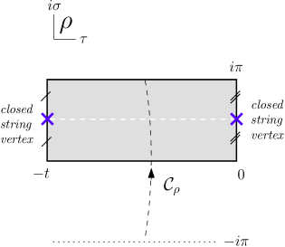
Figure 1: Word-sheet description of two closed string scattering amplitude. Contour $\mathcal{C}_{\rho}$ is a path for ghost integration.

In the last term in (2.3), $|\mathcal{I}\rangle$ is the identity string field which operates as gluing the two halves of the string together. Hence, the open-closed vertex has the following geometrical interpretation: a closed string vertex operator is inserted in the midpoint of the open string and then the two halves of string are sewed together.

3 Two closed string amplitudes

Now using the Feynman rules in the previous section, we can calculate S-matrix elements of any closed or open string. As has been mentioned before, the S-matric element of two closed string tachyon operators has been calculated in [25]. The authors in [25] have used the conformal mapping method to calculate the amplitude exactly. Their result is exactly the same as the scattering amplitude of two closed string tachyons off a D-brane in perturbative string theory. However, in this section we use a conformal map which is slightly different from the one used in [25], and we show that the S-matrix element of ${\it any}$ two closed strings is exactly equal to the corresponding amplitude in perturbative bosonic string theory.

The world-sheet of this scattering is shown in Fig.1. It is simply a finite length strip (open string propagator) where an identity operation acts at each of the two points, $\tau=0$ and $\tau=-t$. The two closed string vertices should be inserted at two singular midpoints. Using the propagator (2.4) one may write the amplitude as :

$$A_{O_{c}O_{c}} = \int_{0}^{\infty}dt\langle V_{12}|b_{0}e^{-tL_{0}^{(2)}}|O_{c}\rangle_{1}|O_{c}\rangle_{2}\;\;,$$ (3.1)

where $|V_{12}\rangle$ is the 2-point vertex operator and $|O_{c}\rangle\equiv V_{O_{c}}(\frac{i\pi}{2})|\mathcal{I}\rangle$ defines a closed string state. The above amplitude can be written in terms of CFT correlation functions in the $\rho$-plane as

$$A_{O_{c}O_{c}} = \int_{0}^{\infty}dt\int_{C_{\rho}}\frac{d\rho}{2\pi i}\langle b_{\rho\rho}(\rho)V_{1O_{c}}(\frac{i\pi}{2})V_{2O_{c}}(\frac{i\pi}{2}-t)\rangle_{\rho}\;\;,$$ (3.2)

where we have used $b_{0}=\int_{\mathcal{C}_{\rho}}\frac{d\rho}{2\pi i}b_{\rho\rho}(\rho)$ and the contour $\mathcal{C}_{\rho}$ is from $-i\pi$ to $i\pi$. In writing this relation we have used the doubling trick $b_{\bar{\rho}\bar{\rho}}(\bar{\rho})=b_{\rho\rho}(\bar{\rho})$ as well. The closed string vertex operator is

$$V_{O_{c}}(\rho) = C(\rho)\bar{C}(\bar{\rho})O_{c}(\rho,\bar{\rho})\;\;,$$ (3.3)

where $O_{c}$ is the matter part of the vertex operator. Using the fact that world-sheet propagators have simple forms in the upper half $z$-plane, one usually maps the world-sheet Fig.1 to the upper half $z$-plane. A map which does this has been given in [25] to calculate the amplitude for two tachyons. However, we will map this world-sheet to the $z$-plane in a slightly different way which makes us able to conclude that the amplitude of any two closed strings is the same as the corresponding amplitude in perturbative string theory.

Figure 2: Half part of the Riemann surface depicted in Fig. 1.

3.1 Conformal mapping

By cutting the Riemann world-sheet along the line joining the two singular pints, we can divide it into two similar rectangles, with no singularity therein. We call them $ABCD$ and $A^{\prime}B^{\prime}C^{\prime}D^{\prime}$. The rectangle $ABCD$ is shown in Fig.2. Gluing segments $BC$ to $B^{\prime}C^{\prime}$, $CD$ to $C^{\prime}D^{\prime}$, and $DA$ to $D^{\prime}A^{\prime}$, one will restore the original world-sheet in Fig.1. The basic idea of mapping the world-sheet to $z$-plane is to find a map which brings the upper right half $z$-plane to the rectangle $ABCD$ and the upper left half $z$-plane to the rectangle $A^{\prime}B^{\prime}C^{\prime}D^{\prime}$ in such a way that the image of segments $BCDA$ and $B^{\prime}C^{\prime}D^{\prime}A^{\prime}$ each separately covers the imaginary axis completely. Since the imaginary axis is common between upper right half $z$-plane and upper left half $z$-plane, this axis shows the gluing part of the original world-sheet in Fig.1.

Now we try to find the map in two steps. Firstly, the Schwarz-Christoffel method tells us how to find the map $\rho(w)$, which brings the upper half $w$-plane into the interior of any polygon, so that the image of real axis covers the circumference of the polygon once. Derivative of this map is $\frac{d\rho}{dw}=\frac{N}{2}\prod_{i=1}^{i=m}(w-w_{i})^{a_{i}}$ where $w_{i}$’s are images of the vertices of the polygon, and $N$ is a constant. Edges of the vertex $i$ rotate through the angle $a_{i}\pi$ which is positive (negative) for counterclockwise (clockwise) direction. For the rectangle $ABCD$ in Fig.2 this becomes

$$\frac{d\rho}{dw} = \frac{N}{2}\frac{1}{\sqrt{w}\sqrt{w+\beta^{2}}\sqrt{w+1}}\;\;,$$ (3.4)

in which we have assumed that points ${\infty}$, ${0}$, ${-\beta^{2}}$, and $-1$ on the $w$-plane are images of vertices ${A}$, ${B}$, ${C}$, and ${D}$, respectively (see Fig.3). Note that the $SL(2,R)$ symmetry of the upper half $w$-plane allows us to set three points fixed. We chose them to be the images of ${A}$ and ${B}$, and $D$. Using the fact that all points at infinity are coincident, the above transformation maps segment $BCDA$ to the negative real axis of the $w$-plane. The square roots in the denominator of (3.4) come from the fact that all edges of the rectangle rotate $\pi/2$ clockwise. We have also absorbed the constant $1/\sqrt{w-\infty}$ in $N$. We shall find the constant $N$ shortly.

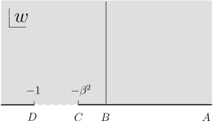
Figure 3: Image of the rectangle depicted in Fig. 2 on the $w$-plane.

The second step is to find a transformation which maps the upper half $w$-plane to the right hand side of the upper half $z$-plane. This map is simply $w=z^{2}$. Combining the two transformations $\rho(w)$ and $w(z)$ will bring the right hand side of the upper half $z$-plane to the rectangle $ABCD$ such that the imaginary axis of the $z$-plane maps to the segment $BCDA$, as required. The map is then,

$$\rho(z) = \int\left(\frac{d\rho}{dw}\right)\left(\frac{dw}{dz}\right)dz$$ (3.5)

$$= N\int^{z}_{z_{0}}\frac{dz}{\sqrt{z^{2}+\beta^{2}}\sqrt{z^{2}+1}}\;\;.$$

As shown in the Fig.4, images of the vertices on the $z$-plane are ${\infty}$, ${0}$, ${i\beta}$, and $i$. In above equation $z_{0}$ is a constant in which we are not interested. The same map will bring the upper left hand side of $z$-plane to the rectangle $A^{\prime}B^{\prime}C^{\prime}D^{\prime}$ in which the imaginary axis is mapped to segment $B^{\prime}C^{\prime}D^{\prime}A^{\prime}$. Therefore, one recovers the original world-sheet in Fig.1 in which the segments $BCDA$ and $B^{\prime}C^{\prime}D^{\prime}A^{\prime}$ are glued together.

To find the constant $N$, we use the fact that the length of segment $BC$ must be equal to $\pi/2$. This gives

$$\rho(i\beta)-\rho(0) = N\int^{i\beta}_{0}\frac{dz}{\sqrt{z^{2}+\beta^{2}}\sqrt{z^{2}+1}}=\frac{i\pi}{2}\;\;.$$

Using the change of variable as $u=z/(i\beta)$, this integral becomes of the form of a complete elliptic integral of the first kind [27]. Hence, one finds,

$$N = \frac{\pi}{2K(m)}\;\;,$$ (3.6)

where $m=\beta^{2}$.

The idea of conformal mapping is to map the positions of all operators in (3.2) to the $z$-plane, and also change the modular parameter $t$ to the modular parameter $\beta$ which is the position of one of the vertex operators. To find this relation between $\beta$ and $t$, we use the fact that the length of segment $CD$ is equal to $t$, that is,

$$\rho(i)-\rho(i\beta) = N\int^{i}_{i\beta}\frac{dz}{\sqrt{z^{2}+\beta^{2}}\sqrt{z^{2}+1}}=t\;\;.$$

Using (3.6) and changing the variable as $u^{2}=(1+z^{2})/(1-\beta^{2})$, one finds an explicit relation,

$$\frac{\pi K(m^{\prime})}{2K(m)} = t\;\;,$$ (3.7)

in which $m^{\prime}=1-m$. It is easy to see that $\beta$ goes to zero when $t\rightarrow\infty$, and goes to one as $t\rightarrow 0$. Using the derivative formula

$$dK(m)/dm=[E(m)-m^{\prime}K(m)]/2mm^{\prime}\;\;,$$ (3.8)

where $E$ is the complete elliptic integral of the second kind, and the Legendre’s relation,

$$E(m^{\prime})K(m)-K(m^{\prime})K(m)+E(m)K(m^{\prime}) = \pi/2\;\;,$$ (3.9)

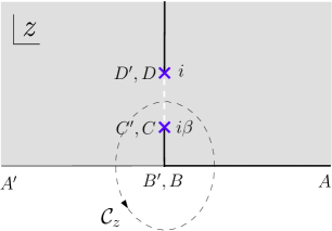
Figure 4: Upper half $z$-plane description of the world-sheet in Fig. 1. The conformal map $(\ref{CCSCT})$ transforms the $z$-plane to the Riemann surface depicted in Fig. 1. Contour $\mathcal{C}_{z}$ is a path for ghost integration.

one can easily differentiate (3.7) to get,

$$dt =- \frac{(\pi/2)^{2}}{K^{2}(m)\beta(1-\beta^{2})}d\beta\;\;.$$ (3.10)

Note that the non trivial function $K(m)$ appears in the Jacobian of the transformation. However, as we shall see shortly, this function does not appear in the final amplitude.

Finally, using the fact that the anti-ghost field $b_{\rho\rho}$ has conformal weight 2, one can write the following transformation:

$$\int_{\mathcal{C}_{\rho}}\frac{d\rho}{2\pi i}b_{\rho\rho}(\rho)=\oint_{\mathcal{C}_{z}}\frac{dz}{2\pi i}\left(\frac{dz}{d\rho}\right)b_{zz}(z)\;\;.$$ (3.11)

Now, using equations (3.11) and (3.10), and using the fact that vertex 1 (2) at point $i\pi/2$ ( $i\pi/2-t$) in the $\rho$-plane is mapped to $i$ ( $i\beta$) in the $z$-plane, one can write the scattering amplitude (3.2) in the $z$-plane as

$$A_{O_{c}O_{c}} = \int_{0}^{1}d\beta\langle O_{1c}(i,-i)O_{2c}(i\beta,-i\beta)\rangle_{z}$$

$$\times \frac{(\pi/2)^{2}}{\beta(1-\beta^{2})K^{2}(m)}\oint_{\mathcal{C}_{z}}\frac{dz}{2\pi i}\left(\frac{dz}{d\rho}\right)\langle C(i)\bar{C}(-i)b(z)C(i\beta)\bar{C}(-i\beta)\rangle_{z}\;\;,$$

where $b(z)=b_{zz}(z)$.

Using the doubling trick $\bar{C}(\bar{z})=C(\bar{z})$, the two-point function $\langle b(z)C(z^{\prime})\rangle=1/(z-z^{\prime})$, and the relation $\langle C(z_{1})C(z_{2})C(z_{3})\rangle=(z_{1}-z_{2})(z_{2}-z_{3})(z_{1}-z_{3})$, one finds

$$\langle C(i)\bar{C}(-i)b(z)C(i\beta)\bar{C}(-i\beta)\rangle_{z} = -\frac{4\beta(1-\beta^{2})^{2}}{(z^{2}+\beta^{2})(z^{2}+1)}\;\;.$$ (3.13)

Inserting this in the integral (3.1), and using equations (3.5) and (3.6), one can perform the z-integration in (3.1). The result is

$$A_{O_{c}O_{c}} =-4 \int_{0}^{1}d\beta\,(1-\beta^{2})\langle O_{1c}(i,-i)O_{2c}(i\beta,-i\beta)\rangle_{z}\;\;,$$ (3.14)

where we have used the formula

$$\frac{1}{2\pi i}\oint_{\mathcal{C}_{z}}\frac{dz}{\sqrt{(z^{2}+\beta^{2})(z^{2}+1)}} = \frac{2}{\pi}\int_{0}^{1}\frac{du}{\sqrt{(1-u^{2})(1-\beta^{2}u^{2})}}$$ (3.15)

$$= \frac{2K(m)}{\pi}\;\;.$$

In finding the above formula, we have used the fact that the contour $\mathcal{C}_{z}$ includes the two singular points $z=i\beta$ and $z=-i\beta$. As we have mentioned before, the function $K(m)$ does not appear in the final amplitude (3.14).

On the other hand, the S-matrix element describing the scattering amplitude of two arbitrary closed string states off a D-brane in perturbative string theory is given by the following correlation function in the $z$-plane:

$$A_{O_{c}O_{c}}\sim\int d^{2}z_{1}d^{2}z_{2}\langle O_{1c}(z_{1},\bar{z}_{1})O_{2c}(z_{2},\bar{z}_{2})\rangle_{z}\;\;.$$ (3.16)

The integrand has SL(2,R) symmetry. Gauging this symmetry by fixing $z_{1}=i$ and $z_{2}=i\beta$, one finds [26]

$$\int d^{2}z_{1}d^{2}z_{2}\longrightarrow\int_{0}^{1}d\beta\,(1-\beta^{2})\;\;.$$ (3.17)

This makes the amplitude (3.16) to be exactly like the amplitude in (3.14). This completes our illustration of the equality between the tree level S-matrix elements involving two arbitrary closed string states in the OSFT and the corresponding disk level S-matrix elements in perturbative string theory.

4 One closed and two open strings amplitudes

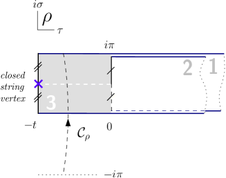
Figure 5: Word-sheet description of one closed and two open string scattering amplitude. Contour $\mathcal{C}_{\rho}$ is a path for ghost integration.

The more involved amplitude is the S-matrix element of one closed and two open strings. World-sheet description for this process is depicted in Fig.5. Two on-shell open strings (semi-infinite strip) and one off-shell open string (finite length strip) are gluing together at $\tau=0$, according to the Witten’s way of joining strings [3]. At time $\tau=-t$, where $t$ is between $0$ and $\infty$, a closed string vertex operator is inserted on the singular midpoint generated by the identity operator acting on string 3. Using the propagator (2.4), one may write the amplitude as:

$$A_{O_{o}O_{o}O_{c}} = \int_{0}^{\infty}dt\langle V_{123}|b_{0}e^{-tL_{0}^{(3)}}|O_{o}\rangle_{1}|O_{o}\rangle_{2}|O_{c}\rangle_{3}\;\;,$$ (4.1)

where $|V_{123}\rangle$ is the 3-point vertex operator, and $|O_{o}\rangle$ is an open string state. The above amplitude can be written in terms of CFT correlation functions in the $\rho$-plane as

$$A_{O_{o}O_{o}O_{c}} = \int_{0}^{\infty}dt\int_{C_{\rho}}\frac{d\rho}{2\pi i}\langle b_{\rho\rho}(\rho)V_{1O_{o}}(\infty)V_{2O_{o}}(\infty)V_{3O_{c}}(\frac{i\pi}{2}-t)\rangle_{\rho}\;\;.$$ (4.2)

The closed string vertex operator is given in (3.3), and the open string vertex operator is

$$V_{O_{o}}(\rho) = C(\rho)O_{o}(\rho)\;\;,$$ (4.3)

where $O_{o}$ is the matter part of the open string vertex operator. Searching for a suitable transformation that maps the world-sheet to the upper half $z$-plane, is a crucial step for performing the above CFT computations. We will follow the same strategy as in the previous section.

4.1 Conformal Mapping

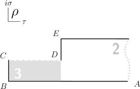
Figure 6: Half part of the Riemann surface depicted in Fig. 5.

As in the two closed strings case, here also we face a Riemann surface with two singular points. By cutting the world-sheet along the line joining the two singular pints, we can divide it into two similar pentagons, with no singularity therein. We call them $ABCDE$ and $A^{\prime}B^{\prime}C^{\prime}D^{\prime}E^{\prime}$. One of these degenerated pentagons is depicted in Fig. 6. Vertex $A$ goes to plus infinity. Joining the two pentagons along the segments $BCDE$ and $B^{\prime}C^{\prime}D^{\prime}E^{\prime}$ will restore the original world sheet. We should find a map $\rho(z)$ which brings the upper right half $z$-plane to one pentagon, so that the image of segment $BCDE$ covers the imaginary axis completely. Again we do it in two steps. By the Schwarz-Christoffel method we can find the map $\rho(w)$, which brings the upper half $w$-plane into the interior of the pentagon. Regarding all exterior angles, one can write

$$\frac{d\rho}{dw} = \frac{N}{2}\frac{\sqrt{w+\alpha^{2}}}{\sqrt{w}\sqrt{w+\beta^{2}}(w-1)}\;\;,$$ (4.4)

in which we assume that points $1$, ${0}$, ${-\beta^{2}}$, ${-\alpha^{2}}$ and ${-\infty}$ on the $w$-plane are images of vertices ${A}$, ${B}$, ${C}$, ${D}$ and ${E}$, respectively ( see Fig.7).

Combining $\rho(w)$ with transformation $w=z^{2}$, one finds $\rho(z)$:

$$\rho(z) = N\int^{z}_{z_{0}}dz\frac{\sqrt{z^{2}+\alpha^{2}}}{\sqrt{z^{2}+\beta^{2}}(z^{2}-1)}\;\;.$$ (4.5)

As shown in the Fig.8, images of the pentagon vertices on the $z$-plane are $1$, ${0}$, ${i\beta}$, ${i\alpha}$ and ${+\infty}$. To find the constant $N$, one may consider the fact that the weight of strip 2 at $A$ must be equal to $\pi$. This gives

$$\int dz(\frac{d\rho}{dz}) = i\pi\;\;,$$

where the integration is taken along a clockwise semi-contour around the point $A$ in the upper half $z$-plane. This indicates that $d\rho/dz$ must have a simple pole at $z=1$,

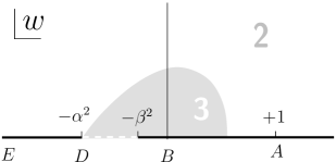
Figure 7: Image of the pentagon depicted in Fig. 6 on the $w$-plane.

$$\frac{d\rho}{dz}|_{z=1} = \frac{-1}{z-1}\;\;.$$

This requirement will fix the factor $N$ to be

$$N = -2\frac{\sqrt{1+\beta^{2}}}{\sqrt{1+\alpha^{2}}}\;\;.$$

For the special case that $\alpha=\beta$, one has a semi-infinite strip which maps to the right hand side of the upper half $z$-plane by $\rho(z)=-\ln(1-z)+\ln(1+z)$. This fixes $z_{0}$ in (4.5) to be $z_{0}=0$. This transformation also maps the mid point of the semi-infinite strip to $z=i$.

The parameters $\alpha$ and $\beta$ are both functions of $t$. Hence there should be a relation between these two parameters. To find this relation, one may consider the condition that the length of segment $BC$ must be $\pi/2$. This leads to the following constraint equation between $\alpha$ and $\beta$:

$$f(\alpha,\beta) = \frac{i\pi}{2}\;\;,$$ (4.6)

where $f(\alpha,\beta)\equiv\rho(i\beta)-\rho(0)$.

Making use of (4.5), one can write $f(\alpha,\beta)$ as

$$f(\alpha,\beta) = N\int^{i\beta}_{0}dz\frac{\sqrt{z^{2}+\alpha^{2}}}{\sqrt{z^{2}+\beta^{2}}(z^{2}-1)}\;\;,$$

which can be rewritten in terms of complete elliptic integrals by using the change of variable $u=z/i\beta$,

$$f(\alpha,\beta)=iN\alpha\left[\frac{1}{\alpha^{2}}\int^{1}_{0}\frac{du}{\sqrt{1-u^{2}}\sqrt{1-mu^{2}}}-(1+\frac{1}{\alpha^{2}})\int^{1}_{0}\frac{du}{\sqrt{1-u^{2}}\sqrt{1-mu^{2}}(1-nu^{2})}\right],$$

where $m=\beta^{2}/\alpha^{2}$ and $n=-\beta^{2}$. The first and second integrals are the standard form of complete elliptic integrals of first and third kind, respectively. Hence,

$$f(\alpha,\beta) = iN\alpha\left[\frac{1}{\alpha^{2}}K(m)-(1+\frac{1}{\alpha^{2}})\Pi(n|m)\right]\;\;.$$

Using the Jacobi formula it is possible to write $\Pi(n|m)$ in terms of elliptic integrals of first and second kind [27]. After some algebra, one gets,

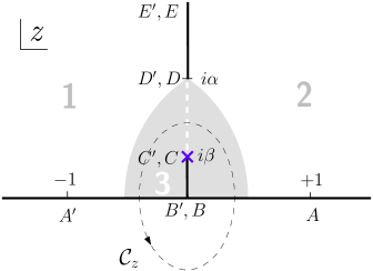
Figure 8: Upper half $z$-plane description of the world-sheet in Fig. 5. The conformal map $(\ref{SCT})$ transforms the $z$-plane to the Riemann surface depicted in Fig. 5. Contour $\mathcal{C}_{z}$ is a path for ghost integration.

$$f(\alpha,\beta) = 2K(m)\left[i\alpha\sqrt{\frac{1+\beta^{2}}{1+\alpha^{2}}}-Z(\phi|m)\right]\;\;,$$

where $Z$ is the Jacobi Zeta function [27] and $\sin{\phi}=i\alpha$.

Another constraint equation which sets relation between $\alpha$, $\beta$ and $t$, comes from the condition that the length of segment $CD$ must be equal to $t$, that is,

$$g(\alpha,\beta) = t\;\;,$$ (4.7)

where $g(\alpha,\beta)\equiv\rho(i\alpha)-\rho(i\beta)$.

Using (4.5), one can write $g(\alpha,\beta)$ as

$$g(\alpha,\beta) = N\int^{i\alpha}_{i\beta}dz\frac{\sqrt{z^{2}+\alpha^{2}}}{\sqrt{z^{2}+\beta^{2}}(z^{2}-1)}\;\;.$$

Again this can be rewritten in terms of complete elliptic integrals using the change of variable $u^{2}=(\alpha^{2}+z^{2})/(\alpha^{2}-\beta^{2})$,

$$g(\alpha,\beta) = \frac{N}{\alpha}\left[\int^{1}_{0}\frac{du}{\sqrt{1-u^{2}}\sqrt{1-m^{\prime}u^{2}}}-\int^{1}_{0}\frac{du}{\sqrt{1-u^{2}}\sqrt{1-m^{\prime}u^{2}}(1-n^{\prime}u^{2})}\right]\;\;$$

$$= \frac{N}{\alpha}\left[K(m^{\prime})-\Pi(n^{\prime}|m^{\prime})\right]\;\;$$

$$= 2K(m^{\prime})Z(\phi^{\prime}|m^{\prime})\;\;,$$

where $m^{\prime}=1-m$, $n^{\prime}=(\alpha^{2}-\beta^{2})/(1+\alpha^{2})$, and $\sin{\phi^{\prime}}=\alpha/\sqrt{1+\alpha^{2}}$. From above relations, one can find the boundary value for $\beta$. This boundary is $\beta\rightarrow 0$ as $t\rightarrow\infty$, and $\beta=\alpha$ at $t=0$. However, as we have shown before, the point $\alpha=\beta$ which is the midpoint of the semi-infinite strip is mapped to $z=i$. Hence, at $t=0$, $\beta\rightarrow 1$.

Making use of the two constraint equations (4.6) and (4.7), one can write the measure factor $dt$ in terms of $d\beta$, that is,

$$dt = \left(\partial_{\beta}g-\frac{\partial_{\beta}f}{\partial_{\alpha}f}\partial_{\alpha}g\right)d\beta\;\;.$$ (4.8)

Using the derivative formulas (3.8) and

$$dZ(\phi|m) = \left\{\frac{1}{2m}\left(1-\frac{E(m)}{m^{\prime}K(m)}\right)Z(\phi|m)+\frac{E(m)\sin(2\phi)}{4m^{\prime}K(m)\sqrt{1-m\sin^{2}(\phi)}}\right\}dm$$ (4.9)

$$+\left\{\sqrt{1-m\sin^{2}(\phi)}-\frac{E(m)}{K(m)\sqrt{1-m\sin^{2}(\phi)}}\right\}d\phi\;\;,$$

one can show, after some algebra, that

$$\partial_{\alpha}g = \frac{2}{1+\alpha^{2}}\sqrt{\frac{1+\beta^{2}}{1+\alpha^{2}}}K(m^{\prime})\;\;,$$

$$\partial_{\beta}g = \frac{-2(\alpha/\beta)}{\sqrt{(1+\alpha^{2})(1+\beta^{2})}}E(m^{\prime})\;\;,$$ (4.10)

$$\partial_{\alpha}f = \frac{2i}{1+\alpha^{2}}\sqrt{\frac{1+\beta^{2}}{1+\alpha^{2}}}K(m)\;\;,$$

$$\partial_{\beta}f = \frac{2i(\alpha/\beta)}{\sqrt{(1+\alpha^{2})(1+\beta^{2})}}\left(E(m)-K(m)\right)\;\;.$$

Inserting (4.10) into (4.8) and using the identity (3.9), one finds the following relation between $dt$ and $d\beta$:

$$dt=-\frac{\pi(\alpha/\beta)}{K(m)\sqrt{(1+\alpha^{2})(1+\beta^{2})}}d\beta\;\;.$$ (4.11)

Now making use of equations (3.11) and (4.11), and use the fact that vertices 1, 2, and 3 are mapped to points -1, 1, and $i\beta$, respectively, one can write the scattering amplitude (4.2) in the $z$-plane as

$$A_{O_{o}O_{o}O_{c}} = \int_{0}^{1}d\beta\langle O_{1o}(-1)O_{2o}(1)O_{3c}(i\beta,-i\beta)\rangle_{z}$$

$$\times \frac{\pi(\alpha/\beta)}{K(m)\sqrt{(1+\alpha^{2})(1+\beta^{2})}}\oint_{\mathcal{C}_{z}}\frac{dz}{2\pi i}\left(\frac{dz}{d\rho}\right)\langle C(-1)C(1)b(z)C(i\beta)\bar{C}(-i\beta)\rangle_{z}\;\;.$$

The correlation in the ghost part can be evaluated. One finds,

$$\langle C(-1)C(1)b(z)C(i\beta)\bar{C}(-i\beta)\rangle_{z} = \frac{4i\beta(1+\beta^{2})^{2}}{(z^{2}+\beta^{2})(1-z^{2})}\;\;.$$ (4.13)

Inserting this into (4.1), using the map (4.5) to evaluate $\frac{dz}{d\rho}$, and performing the z-integration using (3.15), one finds finally

$$A_{O_{o}O_{o}O_{c}} =4i \int_{0}^{1}d\beta\,(1+\beta^{2})\langle O_{1o}(-1)O_{2o}(1)O_{3c}(i\beta,-i\beta)\rangle_{z}\;\;.$$ (4.14)

It is interesting to note that here also the non trivial function $K(m)$ which appears in the measure $dt$ (4.11), is canceled by the same function that results from integration over the ghost correlators. Similar cancellation happens for the S-matrix element of four tachyons too [10].

In the perturbative string theory, on the other side, the S-matrix element describing the decay amplitude of two arbitrary open string states on a D-brane to one arbitrary closed string state is given by the following correlation function in the $z$-plane:

$$A_{O_{o}O_{o}O_{c}}\sim\int dx_{1}dx_{2}d^{2}z_{3}\langle O_{1o}(x_{1})O_{2o}(x_{2})O_{3c}(z_{3},\bar{z}_{3})\rangle_{z}\;\;.$$ (4.15)

The integrand has again SL(2,R) symmetry. Gauging this symmetry by fixing $x_{1}=-1$ $x_{2}=1$, and $z_{3}=i\beta$, one finds [28],

$$\int dx_{1}dx_{2}d^{2}z_{3}\longrightarrow\int_{0}^{1}d\beta\,(1+\beta^{2})\;\;.$$ (4.16)

This makes the amplitude (4.15) to be exactly like the amplitude in (4.14). This completes our illustration of the equality between the tree level S-matrix elements involving one arbitrary closed string and two arbitrary open strings in the OSFT and the corresponding disk level S-matrix elements in perturbative string theory.

It has been shown in [10] that the S-matrix element of four tachyons in the OSFT is identical to the corresponding amplitude in perturbative string theory. Making use of the strategy utilized in the present paper, one can extend that equality to the S-matrix element of four ${\it arbitrary}$ open string states.

Finally, one may try to extend the S-matrix element of one closed and two open strings to the off-shell physics using the method in [11]. The important point is that only open string states can be extended to the off-shell. It is of interest to investigate such an off-shell extension. It would also be interesting to study higher point functions involving the closed string operators.

Acknowledgments: M.R.G would like to thank ICTP for hospitality during the completion of this work. G.R.M was supported by Birjand university. We would like to thank A.E. Mosaffa for critical reading of the manuscript.

References

- [1] K. Ohmori, “A Review on Tachyon Condensation in Open String Field Theories”, hep-th/0102085.
- [2] I.Ya. Aref’eva, D.M. Belov, A.A. Giryavets, A.S. Koshelev and P.B. Medvedev, “Non-commutative Field Theories and (Super)String Field Theories”, hep-th/0111208.
- [3] E. Witten, “Non-commutative geometry and string field theory”, Nucl. Phys. B 268 (1986) 253.
- [4] A. Sen, “ Descent Relations Among Bosonic D-branes”, Int. J. Mod. Phys. A 14 (1999) 4061 [arXiv:hep-th/9902105]; “ Universality of the Tachyon Potential”, JHEP 9912 (1999) 027 [arXiv:hep-th/9911116].
- [5] S.B. Giddings and E. J. Martinec, “Conformal Geometry and String Field Theory”, Nucl. Phys. B278 (1986) 91.
- [6] S.B. Giddings, E.J. Martinec and E. Witten, “Modular Invariance In String Field Theory”, Phys. Lett. B 176 (1986) 362.
- [7] B. Zwiebach, “A Proof That Witten’s Open String Theory Gives A Single Cover Of Moduli Space”, Commun. Math. Phys. 142 (1991) 193.
- [8] W. Taylor, “Perturbative diagrams in string field theory”, arXiv:hep-th/0207132.
- [9] W. Taylor and B. Zwiebach, “D-Branes, Tachyons, and String Field Theory”, arXiv:hep-th/0311017.
- [10] S.B. Giddings, “The Veneziano amplitude from interacting string field theory “, Nucl. Phys. B 278 (1986) 242.
- [11] J.H. Sloan, “The scattering amplitude for four off-shell tachyons from functional integrals ”, Nucl. Phys. B 302 (1988) 349.
- [12] S. Samuel, “Covariant off-shell string amplitudes ”, Nucl. Phys. B 308 (1988) 285.
- [13] S. Samuel, “Solving The Open Bosonic String In Perturbation Theory”, Nucl. Phys. B 341 (1990) 513.
- [14] W. Taylor, “Perturbative computations in string field theory”, arXiv:hep-th/0404102.
- [15] D.Z. Freedman, S.B. Giddings, J.A. Shapiro and C.B. Thorn, “The Nonplanar One Loop Amplitude In Witten’s String Field Theory”, Nucl. Phys. B 298 (1988) 253.
- [16] W. Taylor , “Tadpoles and Closed String Backgrounds in Open String Field Theory”, JHEP 0307 (2003) 059 [arXiv:hep-th/0304259].
- [17] H. Terao and S. Uehara, “On the dilaton vertex in the Covariant Formulation of String”, Phys. Lett. B188 (1987) 198.
- [18] J. A. Shapiro and C. B. Thorn, “BRST invariant Transition between Closed and Open String”, Phys. Rev. D36 (1987) 432, and “Closed String-Open String Transition and Witten’s String Field Theory”, Phys. Lett. B194 (1987) 43.
- [19] A. Strominger, “Closed String in Open String Field Theory”, Phys. Rev. Lett. 16 (1987) 629.
- [20] B. Zwiebach, “Interpolation String Field Theories”, Mod. Phys. Lett. A7 (1992) 1079; hep-th/9202015.
- [21] A. Hashimoto and N. Itzhaki, “Observable of String Field Theory”, JHEP 0201 (2002) 028 [arXiv:hep-th/0111092].
- [22] D. Gaiotto, L. Rastelli, A. Sen and B. Zwiebach, “Ghost Structure and Closed Strings in Vacuum String Field Theory”, Adv. Theor. Math. Phys. 6 (2002) 403 [arXiv:hep-th/0111129].
- [23] M. Alishahiha and M.R. Garousi, “Gauge Invariant Operators and Closed String Scattering in Open String Field Theory”, Phys. Lett. B 536 (2002) 129 [arXiv:hep-th/0201249].
- [24] M.R. Garousi and G.R. Maktabdaran, “Excited D-brane decay in Cubic String Field Theory and in Bosonic String Theory”, Nucl. Phys. B651 (2003) 26 [arXiv:hep-th/0210139].
- [25] T. Takahashi and S. Zeze, “Closed Sting Amplitude In Open String Field Theory”, JHEP 0308 (2003) 020 [arXiv:hep-th/0307173].
- [26] M.R. Garousi and R.C. Myers, Nucl. Phys. B475 (1996) 193 [arXiv:hep-th/9603194].
-
[27]
M. Abramowitz, I.A. Stegun, “Handbook of Mathematical Functions,
With Formulas, Graphs, and Mathematical Tables”, Dover
Publications, INC., New York (1974).
For a online library, see “The Wolfram Function Site” at http://functions.wolfram.com. - [28] A. Hashimoto, I.R. Klebanov, Phys. Lett. B 381 (1996) 437; [arXiv:hep-th/9604065].