Coexistence of black holes and a long-range scalar field in cosmology

Abstract

The exactly solvable scalar hairy black hole model (originated from the modern high-energy theory) is proposed. It turns out that the existence of black holes (BH) is strongly correlated to global scalar field, in a sense that they mutually impose bounds upon their physical parameters like the BH mass (lower bound) or the cosmological constant (upper bound). We consider the same model also as a cosmological one and show that it agrees with recent experimental data; additionally, it provides a unified quintessence-like description of dark energy and dark matter.

Two of the most fundamental predictions of the modern high-energy theory and gravity are black holes and cosmological scalar field (SF). However, if existence of BH’s has been experimentally confirmed since 70’s (and we even know now that BH’s exist in centers of many galaxies including ours) then the global SF still lacks for direct experimental evidence, mostly due to its extremely weak interaction with other matter. In view of this, here we demonstrate that the good way to proceed would be to search for an influence the SF exerts on the first of the two phenomena we are considering here, black holes.

If one expects that the global ubiquitous scalar field does exist such that everything, including black holes, is “floating” inside it, then one must allow the field to get arbitrarily close to the surface of every BH which exists in the Universe at this moment. Moreover, to keep things physically consistent, when constructing models one must require that SF must be regular in the arbitrarily close vicinity of the event horizon. This requirement, for a first look so innocent, in practice gave rise to enormous technical difficulties. In fact, beginning from 60’s and until recently, nobody has succeeded in satisfying it, i.e., in finding the regular configurations of non-charged black holes and SF, the so-called scalar black holes (SBH). By the latter one assumes the solution which is: (i) possessing an event horizon, (ii) physically acceptable (i.e., both the spacetime and SF must be regular on and outside the horizon, have standard spherical topology and finite physical characteristics like mass, energy density, etc.; also the non-minimal coupling, if any, must obey the recent observational bounds Will:2001mx ), and (iii) not reducible to any other BH existing in absence of SF. All these requirements have not yet been fulfilled, despite the tremendous efforts and certain encouraging results Bocharova:1970 ; Bekenstein:1974sf , see Ref. Martinez:2004nb for the most recent state of the art. The models proposed so far either have unphysical features, like irregularities or exotic topology, or they involve additional gauge fields, and then it becomes not clear why all BH’s should have non-compensated gauge charges to be consistent with global SF. Even the numerical results are rare Torii:2001pg ; Nucamendi:2003ex ; Hertog:2004dr . Not without a sense of irony, people happened to be much more successful in solving the opposite task: finding the requirements under which the physically admissible SBH can not exist, known as the scalar “no-hair” theorems Bizon:1994dh , originated from the Wheeler’s conjecture that a BH can not be characterized by any parameters other than mass, electric charge and angular moment Ruffini:1971 . On the contrary, here we are going to solve this long-standing problem: we present the model which completely satisfies the above-mentioned SBH criteria and thus ultimately falsifies the conjecture.

The model. We use the units where $16\pi G=c=1$, where $G$ is the Newton constant, and consider theory describing self-interacting scalar field $\phi$ minimally coupled to Einstein gravity. Its Lagrangian is ${\cal L}\sim R-(1/2)(\partial\phi)^{2}-V(\phi),$ where the SF potential is given by

$$V=2\lambda(\cosh\phi+2)+4\chi(3\sinh\phi-\phi(\cosh\phi+2)),$$ (1)

where $\chi$ and $\lambda$ are parameters of the model, $\lambda$ is usually called the cosmological constant. The model has the static spherically symmetric solution given in static observer coordinates $\{t,r,\theta,\varphi\}$ by

$$ds^{2}=-N^{2}dt^{2}+\frac{dr^{2}}{N^{2}}+R^{2}(d\theta^{2}+\sin^{2}\!\theta\,d\varphi^{2}),\ e^{\phi}=H,$$ (2)

where $H=1+\kappa/r^{\tilde{d}}$ is a harmonic function, with $\tilde{d}=1$ in our case, $N^{2}=1-2\chi\left[\kappa(r+\kappa/2)-R^{2}\ln H\right]-\lambda R^{2}$ with $R=\sqrt{r(r+\kappa)}$ being the habitual radius and $\kappa$ being the integration constant. The solution was obtained using the separability approach Zloshchastiev:2001da ; Zloshchastiev:2001mw . The model also admits another solution which can be deduced from (2) by the simultaneous inversion $\{\phi\to-\phi,\chi\to-\chi\}$ because our initial Lagrangian has such $Z_{2}$ symmetry. In other words, these two solutions can be grouped into a sort of duplet whose components are characterized by the discrete “charge” $Q\equiv\phi/|\phi|=\pm 1$. For brevity, here we will work only with the solution we started from, corresponding to $Q=1$. To clear its physical meaning, let us expand $N^{2}$ in series assuming $R/\kappa\propto r/\kappa\gg 1$ that gives the Newtonian limit. We get $N^{2}\propto 1-\lambda R^{2}-\frac{2M}{R}+\frac{\chi\kappa^{5}}{40R^{3}}+O(1/R^{5}),$ where we have identified $M=\chi\kappa^{3}/6$ as a gravitating mass of (2). Thus, depending on whether $\lambda$ is zero, positive or negative, our solution is asymptotically flat, de Sitter (dS) or anti-de Sitter (AdS). Note, that the solution can not be reduced to the Schwarzschild one as the limit where SF vanishes corresponds to the de Sitter spacetime.

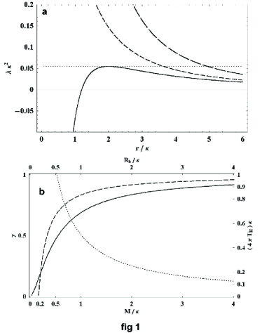
Figure 1: (a) Graphical solution of the horizon equation. The intersections of curves with horizontal lines $\lambda\kappa^{2}$ yield the radii of horizons. Cases: $\gamma\leqslant 0$ (short-dashed curve, plotted at $\gamma=-0.1$); $\gamma>1$ (long-dashed curve, plotted at $\gamma=1.1$); $0<\gamma<1$ (solid curve, plotted at $\gamma=0.8$) where the dotted horizontal line is $\lambda=\lambda_{c}$. In all cases we have at least one horizon (the cosmological one) but only in the third case we have the second, event, horizon. (b) Radius, mass, temperature (here we assume $\lambda$ being negligibly small). The solid and dashed curves correspond, respectively, to the radius $R_{h}$ and mass $M$ as functions of $\gamma$, the dotted curve shows Hawking temperature $T_{H}$ as a function of $M$.

Further, both SF and curvature invariants become singular at $R_{s}=0$, therefore, we may have problems with the Cosmic Censor unless the spacetime has the event horizon located somewhere at $R_{h}=\sqrt{r_{h}(r_{h}+\kappa)}>R_{s}$ thus “dressing” the (otherwise naked) singularity. The horizon condition is $N^{2}(r_{h})=0$, and its graphical solution is shown in Fig. 1a where we have defined $\gamma\equiv 1-(\chi\kappa^{2})^{-1}\not=1$. From there one can deduce a few important things. First, (2) does describe SBH though not for every $\chi$ and $\kappa$ but only for those obeying the inequality

$$0<\gamma<1.$$ (3)

Second, there exists an upper bound for $\lambda$: cosmological constant must be below certain critical value $\lambda_{c}$ otherwise no black hole can exist. Moreover, its absolute value must be much smaller than $\lambda_{c}$ to have the radius of a black hole much less than the size of the observable Universe: $\lambda\ll\lambda_{c}\equiv 4\kappa^{-2}\left(\frac{\ln(2/\gamma-1)}{2(1-\gamma)}-1\right).$ Rough estimates give $\lambda/\lambda_{c}\sim R_{\text{BH}}^{2}/R_{\text{Univ}}^{2}\lesssim 10^{-28}$ if for maximal value of $R_{\text{BH}}$ we take that of the central-galactic BH’s having mass $\lesssim 10^{9}M_{\odot}$. Thus, we see that the global parameter, cosmological constant, turns out to be correlated with local quantities like the size of SBH or its mass. Third, from (3) one can directly derive that the previously defined mass of SBH $M$ is bounded from below: $M\geqslant M_{\text{extr}}\equiv M|_{\gamma\to+0}=\kappa/6,$ also $\gamma$ can be rewritten as $1-M_{\text{extr}}/M$. This property drastically differs SBH from the common BH solutions like the Schwarzschild one where the lower bound is zero. Fourth, (3) also gives the bounds for $\chi$ and $\kappa$: $\chi\geqslant\kappa^{-2}>0$. The joint plot of the most important local characteristics of our SBH (horizon radius, mass and Hawking temperature) is given in Fig. 1b. One can clearly see that when the horizon radius $R_{h}$ approaches zero the mass takes a non-zero value.

Finally, one should not forget that in the presence of SF the Schwarzschild solution can not be regarded as a realistic one because the true vacuum (with vanishing stress-energy tensor $T_{\mu\nu}$) must be replaced by the SF background with $T_{\mu\nu}=\partial_{\mu}\phi\,\partial_{\nu}\phi-g_{\mu\nu}\left[(1/2)(\partial\phi)^{2}+V(\phi)\right]$. In other words, the solutions like (2) should be regarded as describing the actual exterior gravitational field of massive bodies in “vacuum”.

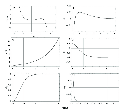
Figure 2: Cosmological scenario A. For all plots except a the horizontal axis is the time measured in units $H_{0}^{-1}\sim 15$ billions years, and zero corresponds to today. The numerical input data: ID $\equiv$ $\{\lambda/\rho_{c},\,\chi/\rho_{c},\,\phi|_{\tau=0},\,(d\phi/d\tau)_{\tau=0}\}$ $=$ $\{0.12,\,0.12,\,10^{-2},\,0\}$, where $\rho_{c}\sim 10^{-29}\,\text{g cm}^{-3}$ is the critical density. We plot: (b) evolution of SF, (c) evolution of the size of the Universe, (d) the deceleration parameter $q=-a\,\ddot{a}/\dot{a}^{2}$, (e) the dark energy ratio $\rho_{\phi}/\rho_{\text{tot}}$, (f) the effective equation of state for SF $p_{\phi}/\rho_{\phi}$.

BH-compatible cosmology. As long as we assume our SF being global and fundamental we must study cosmological consequences the model (1) implies. The potential (1) consists of the symmetric and antisymmetric parts with respect to inversion of $\phi$, proportional to $\lambda$ and $\chi$, respectively. At small $\phi$ and non-zero cosmological constant $\lambda$ the symmetric part dominates: $V(\phi\to 0)\propto 6\lambda(1+\phi^{2}/6)+O(\phi^{4})$, whereas for large values of the field it is the antisymmetric part that brings the main contribution: $V(\phi\to\pm\infty)\propto-2\chi\phi\exp|\phi|$. Following the standard procedure adopted in cosmology we consider SF as a homogenous and isotropic function of cosmological time, $\phi(t)$, and conduct numerical simulations for our model at different values of its parameters. They showed that the following scenarios of the spatially flat FRW Universe evolution are possible.

In the mainstream cosmological scenario with positive $\lambda$, our SF (inflaton) starts at $\phi\ll-1$, rolls down towards the local dS minimum of the potential, passes it and tries to climb over the local dS maximum. If its initial energy is not sufficient to do that (note that the inflaton’s motion is not “frictionless”: there exists sufficient dissipation of energy for creation of radiation and matter) then we have the Scenario A: inflaton rolls back to the local minimum asymptotically approaching the value $\phi=0$, as in Fig. 2b. Meanwhile, the Universe experiences an accelerated expansion, see Fig. 2b, with the eternal acceleration, Fig. 2c. The ratio of the SF density (dark energy) to the total energy density approaches the approximate value $0.72$, Fig. 2d. Figure 2f reveals the quintessential-like Zlatev:1998tr behavior of SF: during some epoch in past (or, equivalently, in “redshifted” regions) it behaved like a pressureless matter ($w_{\phi}\equiv p_{\phi}/\rho_{\phi}\sim 0$) but afterwards its effective equation of state became of the false vacuum type ($w_{\phi}\to w_{\text{DE}}=-1$). Thus, the model provides a unified description of dark energy and dark matter without ad hoc assumptions - they appear to be different manifestations of the same entity, scalar field. All these results agree with the recent experimental data coming from high-redshift observations of supernovae Garnavich:1997nb ; Riess:1998cb ; Perlmutter:1998np and anistropies of the cosmic microwave background (CMB) spectrum Dodelson:1999am ; Netterfield:2001yq ; Stompor:2001xf ; Halverson:2001yy .

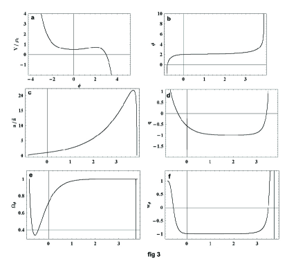
Figure 3: Cosmological scenario B. Notations are the same as in previous Fig.; ID $=$ $\{0.08,\,0.08,\,2,\,0.2\}$.

In another case, when the initial energy of SF is sufficient to overcome the local maximum (classically or by virtue of the tunnelling effect), we have the Scenario B: scalar field rolls over the maximum and starts moving all the way down (Fig. 3b), whereas the Universe at some point begins to decelerate (Fig. 3d), and eventually collapses to the Big Crunch (Fig. 3c), even despite being spatially flat. Figure 3e shows that this scenario is in agreement with experiment too. Thus, one may wonder which scenario is the real one, A (ever-expanding Universe) or B (Big Crunch)? At the classical level - we do not know as we do not know the recent value of SF and its rate of change which are related to the initial ones. The taking into account quantum tunnelling makes Big Crunch an inevitable final state, as will be discussed below.

In principle, the presented scenarios are sufficient to show the viability of the cosmological model based on Eq. (1). Yet, we would like to consider also other possibility - when $\lambda$ is not necessarily positive. The reason is that many people associate the accelerated expansion of the Universe with a positive cosmological constant and the regime where scalar field approaches the dS vacuum state. Let us demonstrate how this stereotype gets broken in our model. By numerical simulations one can easily show that the accelerated expansion of the Universe may occur not only when $\lambda>0$ but also at $\lambda\leqslant 0$, when no dS extrema exist. Let us consider the case $\lambda=0$ only, because the case of a negative cosmological constant (AdS) is very similar qualitatively. In this case the potential has a saddle point at $\phi=0$ instead of two local extrema, see Fig. 4a. One can imagine the following two scenarios. First takes place when the initial value of SF is large negative such that initially it “sits uphill” and starts unbounded motion all the way down, as time goes. Second one happens when initially $\phi$ is situated “downhill” (such that it is large positive) but its initial kinetic energy is large enough to climb up. Then it moves up, passes the saddle point, continues an ascent until reaches the maximum point of its trajectory, and then rolls back all the way down, see Fig. 4 b. The accelerated expansion of the Universe takes place in both cases. However, in the first case the inflation ends too soon such that one could not detect any acceleration nowadays, neither the dark energy approaches its experimentally established value today. The second scenario is better in this connection: the Universe passes a certain epoch of accelerated expansion whose time can be tuned to coincide with today, Fig. 4d. Thereby the size of the Universe evolves with time as in Fig. 4c: decelerated expansion, accelerated expansion, again decelerated expansion, shrinking, and finally, Big Crunch. The recent value of $\Omega_{\phi}$ agrees with experiment, Fig. 4e.

To summarize, our BH-compatible cosmological model (1) seems to be compatible with the experimental data for large range of its parameters. Besides, above our model has been explicitly proven to be consistent with the existence of black holes in the Universe. The class of such models can not be vast a priori because the scalar “no-hair” theorems forbid the appearance of black holes for a large set of the SF potentials, e.g., convex or positive semi-definite Bekenstein:1972ny ; Sudarsky:1995zg . Thus, the existence of BH’s can be the strong criterion for theoretical cosmology sufficiently narrowing the class of physically admissible models.

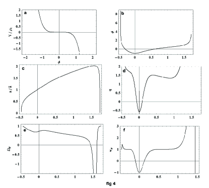
Figure 4: Scenario with $\lambda=0$. ID $=$ $\{0,\,10.3,\,-1,0\}$.

Origin of the model. There is nothing wrong in regarding our model as a postulated one, yet the picture would not be complete without mentioning where (1) came from. It appears in the novel class of the four-dimensional (4D) effective field theories (EFT) which describe the low-energy limit of the 11D M-theory taking into account the non-perturbative aspects such as BPS states and $p$-branes Zlosh . The scalar potential in those EFT’s in the simplest case satisfies the second order differential equation: $V^{\prime\prime}-(a+a^{-1})\coth\left[(a+a^{-1})\phi/4\right]V^{\prime}+V=0,$ where the constant $a$ is precisely the one that appears in the truncated supergravity (SUGRA), ${\cal L}\sim R-(1/2)(\partial\phi)^{2}-(1/2n!)\text{e}^{a\phi}F^{2}_{[n]}+...$ . The potential (1) arises as a solution of this ODE at $a^{2}=1$ (other potentially supersymmetric cases $a^{2}=3,\,1/3$ also have been studied by author but are not listed here). The considering those EFT’s goes far beyond the scope of this paper, instead we just briefly outline some common features of our model and SUGRAs. For instance, the structure of the solution (2) looks very similar to that of $0$-branes Duff:1996hp ; Stelle:1998xg . The Breitenlohner-Freedman parameter Breitenlohner:1982bm takes the conformal value $\mu^{2}=-2>-9/4$ thus the model’s stability can be enhanced by partially unbroken supersymmetry. Further, the symmetric $\lambda$-part of our potential resembles those arising in SUGRA-inspired cosmologies Hertog:2004dr ; DL:1999 ; Kallosh:2001gr , however, our model also has the antisymmetric $\chi$ part which is responsible for black holes (and at the same time for cosmological behavior at large values of SF). Besides, the $\chi$ part is appreciated by string theory and QFT in curved spacetime because of certain conceptual difficulties with the ever-accelerating dS Universe Sasaki:1992ux ; Banks:2001yp . From the quantum viewpoint, even in the Scenario $A$ the local (dS) minimum is a quasi-bound state and thus the system can stay there only for a finite time - eventually it tunnels through the local maximum, such that its further dynamics will be as in Scenario $B$.

- (1) C. M. Will, Living Rev. Rel. 4, 4 (2001).
- (2) N. Bocharova, K. Bronnikov, and V. Melnikov, Vestn. Mosk. Univ., Fiz., Astron. 6, 706 (1970).
- (3) J. D. Bekenstein, Annals Phys. 82, 535 (1974).
- (4) C. Martinez, R. Troncoso and J. Zanelli, Phys. Rev. D 70, 084035 (2004). (they found a BH but with exotic topology)
- (5) T. Torii, K. Maeda and M. Narita, Phys. Rev. D 64, 044007 (2001).
- (6) U. Nucamendi and M. Salgado, Phys. Rev. D 68, 044026 (2003).
- (7) T. Hertog and K. Maeda, JHEP 0407, 051 (2004).
- (8) P. Bizon, Acta Phys. Polon. B 25, 877 (1994).
- (9) R. Ruffini and J. A. Wheeler, Phys. Today 24 (1), 30-41 (1971).
- (10) K. G. Zloshchastiev, Phys. Rev. D 64, 084026 (2001).
- (11) K. G. Zloshchastiev, Phys. Lett. B 527, 215 (2002).
- (12) I. Zlatev, L. M. Wang and P. J. Steinhardt, Phys. Rev. Lett. 82, 896 (1999)
- (13) P. M. Garnavich et al., Astrophys. J. 493, L53 (1998).
- (14) A. G. Riess et al., Astron. J. 116, 1009 (1998).
- (15) S. Perlmutter et al., Astrophys. J. 517, 565 (1999).
- (16) S. Dodelson and L. Knox, Phys. Rev. Lett. 84, 3523 (2000).
- (17) C. B. Netterfield et al., Astrophys. J. 571, 604 (2002).
- (18) R. Stompor et al., Astrophys. J. 561, L7 (2001).
- (19) N. W. Halverson et al., Astrophys. J. 568, 38 (2002).
- (20) J. D. Bekenstein, Phys. Rev. Lett. 28, 452 (1972).
- (21) D. Sudarsky, Class. Quant. Grav. 12, 579 (1995).
- (22) K. G. Zloshchastiev, “An alternative approach to deriving the low-energy limit of M-theory: Getting rid of the ambiguity of dimensional reduction”, in preparation.
- (23) M. J. Duff, H. Lu and C. N. Pope, Phys. Lett. B 382, 73 (1996).
- (24) K. S. Stelle, arXiv:hep-th/9803116.
- (25) P. Breitenlohner and D. Z. Freedman, Phys. Lett. B 115, 197 (1982).
- (26) M. J. Duff and J. T. Liu, Nucl. Phys. B 554, 237 (1999).
- (27) R. Kallosh, A. D. Linde, S. Prokushkin and M. Shmakova, Phys. Rev. D 65, 105016 (2002).
- (28) M. Sasaki, H. Suzuki, K. Yamamoto and J. Yokoyama, Class. Quant. Grav. 10, L55 (1993).
- (29) T. Banks and W. Fischler, arXiv:hep-th/0102077.