USC-04-06

DCPT–04/27

Unoriented Minimal Type 0 Strings

James E. Carlisle^♯ and Clifford V. Johnson^♮

^♯Centre for Particle Theory

Department of Mathematical Sciences

University of Durham

Durham DH1 3LE, England, U.K.

j.e.carlisle@durham.ac.uk

^♮Department of Physics and Astronomy

University of Southern California

Los Angeles, CA 90089-0484, U.S.A.

johnson1@usc.edu

Abstract

We define a family of string equations with perturbative expansions that admit an interpretation as an unoriented minimal string theory with background D–branes and R–R fluxes. The theory also has a well–defined non–perturbative sector and we expect it to have a continuum interpretation as an orientifold projection of the non–critical type 0A string for ${\hat{c}}=0$, the $(2,4)$ model. There is a second perturbative region which is consistent with an interpretation in terms of background R–R fluxes. We identify a natural parameter in the formulation that we speculate may have an interpretation as characterizing the contribution of a new type of background D–brane. There is a non–perturbative map to a family of string equations which we expect to be the $\hat{c}=0$ type 0B string. The map exchanges D–branes and R–R fluxes. We present the general structure of the string equations for the $(2,4k)$ type 0A models.

In what follows, we define a family of theories that have perturbative expansions that admit interpretations as unoriented type 0A string in the $(2,4k)$ superconformal minimal model backgrounds, with D–branes and R–R fluxes. The definitions have a well–defined non–perturbative regime. For the case of ${\hat{c}}=0$, pure supergravity (the $(2,4)$ model) we will see that there is a map to a system which has already been found in the literature, arising from studying self–dual unitary matrix models in the double scaling limit[1]. We argue that it is natural to identify this system as an unorientable type 0B string, the pure supergravity case for that theory.

The string equation for the $k=2$ member of the bosonic minimal string theory for the $(2,2k-1)$ series can be written as[2, 3, 4]:

$$-\frac{1}{3}f^{{}^{\prime\prime}}+f^{2}=z\ ,$$ (1)

where a prime denotes $\nu\partial/\partial z$. This is the Painlevé I equation. Expanding about the large positive $z$ regime gives a well defined perturbation theory representing an oriented bosonic string theory that is in fact pure gravity, i.e. the Liouville theory, since $c=0$ for the matter theory. The free energy is related to $f$ as $F^{{}^{\prime\prime}}=-f$. This model can be realized as the double scaling limit of a one Hermitian matrix model.

In refs.[5, 6, 7, 8], symmetric matrix models (orthogonal and symplectic) were studied in the double scaling limit, and these gave rise to continuum models with contributions from non–orientable world sheets. The physics is then encoded in two functions. The oriented contributions come from $f$ as before, which (for the $k=2$ case) satisfies equation (1), and the unoriented contributions come from a new function, $g$, which satisfies (for this $k=2$ case) the equation:

$$g^{3}+6gg^{{}^{\prime}}+4g^{{}^{\prime\prime}}-6gf-6f^{{}^{\prime}}=0\ .$$ (2)

Given the solution of (1), equation (2) yields three possible solutions for the asymptotic expansion of $g(z)$. We have:

$$f(z) = \sqrt{z}-{\frac{{\nu}^{2}}{24{z}^{2}}}-{\frac{49{\nu}^{4}}{1152{z}^{9/2}}}+\cdots$$

$$g_{1}(z) = \pm\sqrt{6}z^{1/4}-{\frac{\nu}{2z}}\mp{\frac{5{\nu}^{2}\sqrt{6}}{24{z}^{9/4}}}+\cdots$$

$$g_{2}(z) = -{\frac{\nu}{2z}}-{\frac{25{\nu}^{3}}{24{z}^{7/2}}}-{\frac{15745{\nu}^{5}}{1152{z}^{6}}}+\cdots\$$ (3)

and the free energy of the model is given as the sum of an oriented contribution and an unoriented one:

$$F=F_{o}+F_{u}\ ,\quad{\rm where}\quad F_{\mathrm{o}}^{\prime\prime}=-\frac{1}{2}f\>,\qquad F_{\mathrm{u}}^{\prime}=-\frac{1}{2}g\ .$$ (4)

Half of the oriented theory’s free energy makes up the oriented contribution to the free energy of the model. The remainder comes from $g$. Unitary matrix models also have critical points, and in a double scaling limit performed in ref.[9, 10] for the simplest critical point, the following equation can be derived:

$$h^{3}-h^{{}^{\prime\prime}}-hz=0\ ,$$ (5)

which is the Painlevé II equation. For large positive $z$, $h$ has an expansion with an interpretation in terms of oriented world sheets. In fact, this model has recently been understood to be pure supergravity for the type 0B string theory[11], the $k=1$ member of the superconformal series $(2,4k)$.

In ref.[1] self–dual unitary matrix models were studied. It was found that there are again two contributions to the partition function, one coming from orientable surfaces, $h$, which satisfies equation (5); and the other, unorientable contribution, from a function, $w$, which satisfies the Riccati–type equation:

$$w^{{}^{\prime}}=\frac{1}{4}w^{2}+z-\frac{3}{2}h^{2}\ .$$ (6)

Again, the free energy splits into two parts:

$$F=F_{o}+F_{u}\ ,\quad{\rm where}\quad F_{\mathrm{o}}^{\prime\prime}=-\frac{1}{2}h^{2}\>,\qquad F_{\mathrm{u}}^{\prime}=\frac{1}{2}w\ .$$ (7)

It is natural to suppose (and so we propose that it is the case) that this is an unoriented string theory based upon some projection of the 0B theory for ${\hat{c}}=0$. Half of the free energy of the oriented theory makes up the oriented sector of this new theory, and the rest is made up of unoriented contributions.

As is by now very familiar, the physics of the even $k$ minimal bosonic string models (of which equation (1) is the case $k=2$) suffers from a non–perturbative instability, as can be seen from the well–known behaviour of solutions of the equation for $f$. The unoriented theory simply inherits this behaviour.

It is known that there is a family of models that have the same perturbative behaviour as the string equations for the bosonic minimal models; but have better non–perturbative behaviour, defining a family of non–perturbatively stable oriented minimal string theories with the same perturbative content. An example equation is:

$$f{\cal R}^{2}-\frac{1}{2}{\cal R}{\cal R}^{{}^{\prime\prime}}+\frac{1}{4}({\cal R}^{{}^{\prime}})^{2}=\nu^{2}\Gamma^{2}\ .$$ (8)

where

$${\cal R}\equiv-\frac{1}{3}f^{{}^{\prime\prime}}+f^{2}-z\ ,$$ (9)

and for $\Gamma=0$ they have the same large positive $z$ expansion as equation (1). This follows from the fact that ${\cal R}=0$ is a solution to the equation when $\Gamma=0$. There are solutions that solve the equation (8) which are not solutions of ${\cal R}=0$ however, but nevertheless have the same large positive $z$ asymptotic expansions as the solutions of ${\cal R}=0$. These solutions define theories with well–defined non–perturbative physics[12, 13]; and they have now been identified[11] as the type 0A minimal string theories, for the $(2,4k)$ series. The case we have given above is in fact $k=2$. The string equation above captures more than that however[14]. For $\Gamma\neq 0$ it includes a new feature. For large positive $z$, the parameter $\Gamma$ corresponds to there being $\Gamma$ D–branes in the background[14], while for large negative $z$ it corresponds to $\Gamma$ half–units of R–R flux[11].

The simplest model is in fact the choice $k=1$, which is pure type 0A world–sheet supergravity, and has:

$${\cal R}\equiv f-z\ ,$$ (10)

In fact, the case $k=1$ is very special. There is a change of variables[15] which takes the equation (8) (with ${\cal R}$ given in equation (10), and with $\Gamma=0$ (for now)) and maps it to the equation (5). The map is:

$$f=h^{2}+z\ ,$$ (11)

together with the exchange $z\to-z$. This means, as first pointed out in ref.[11], that the physics of pure 0A supergravity and pure 0B supergravity are non–perturbatively related. Non–perturbative because these systems each have two distinct asymptotic regimes, large positive $z$ and large negative $z$ which are separated by a strongly coupled regime. The map above exchanges these regimes. More generally, for non–zero $\Gamma$, the map in equation (11), together with $z\to-z$, takes the 0A string equation (8) to a generalization[11] of the string equation (5):

$$h^{3}-h^{{}^{\prime\prime}}-hz-\frac{\nu^{2}\Gamma^{2}}{h^{3}}=0\ ,$$ (12)

which, for the type 0B model now, has an interpretation in terms of having $\Gamma$ background D–branes in one perturbative regime and $\Gamma$ units of flux in the opposite perturbative regime.

A natural question to ask is whether these 0A equations have a generalization to include an interpretation of the presence of non–orientable surfaces in (at least one of) the perturbative regimes. We shall now show that there is a very natural generalization to include this interpretation.

First, we digress a short while to introduce an elegant differential operator language in which the non–orientable world–sheet physics of the bosonic matrix models can be cast[7]. The basic object in terms of which everything follows is the operator:

$$Q=d^{2}-f(z)\ ,\quad{\rm where}\quad d\equiv\nu{\partial\over\partial z}\ .$$ (13)

For the $k$th bosonic model, one forms the following truncation of a fractional power of $Q$, which we shall denote[17] as $P$:

$$P=Q^{k-\frac{1}{2}}_{+}\ .$$ (14)

The fractional power is defined by requiring that there exist an operator $Q^{\frac{1}{2}}$ such that it squares to give $Q$. In doing this, one needs a definition of $d^{-1}$, and this is such that[18, 19]:

$$d^{-1}f=fd^{-1}+\sum_{i=1}^{\infty}(-1)^{i}f^{(i)}d^{i}\ ,$$ (15)

where $f^{(i)}$ means the $i$th $z$–derivative of $f$. The plus sign subscript in the equation (14) above means that we take only positive powers of $d$. The string equations are formulated as the realization of the fundamental relation[17]:

$$[P,Q]=1\ ,$$ (16)

where one integrates once with respect to $z$ to get the final string equation. In the case of $k=2$ we have:

$$P=d^{3}-\frac{3}{4}\left\{d,f\right\}\ ,$$ (17)

which leads to equation (1). The unoriented sector is defined in terms of the above objects as follows. Require that $P$ be factorizable into the following form:

$$P=(d^{2}+\frac{1}{2}gd+h)(d-\frac{1}{2}g)\ ,$$ (18)

leading to two equations, which when combined give equation (2). We point out here that equation (2) can be written as

$$T^{{}^{\prime}}+gT=0\ ,$$ (19)

where

$$T\equiv g^{{}^{\prime}}+\frac{1}{4}g^{2}-\frac{3}{2}f\ .$$ (20)

A natural sub–family of solutions are those which satisfy $T=0$, which is the following Riccati–type equation:

$$f=\frac{1}{6}g^{2}+\frac{2}{3}g^{{}^{\prime}}\ .$$ (21)

In fact, as pointed out in ref.[5], studying the equation (21) is equivalent to the more restrictive factorization of $P$:

$$P=(d+\frac{1}{2}g)d(d-\frac{1}{2}g)\ .$$ (22)

It turns out that the $g_{1}(z)$ perturbative expansions from equation (3) are the solutions to the $T\!\!=\!0$ equation; whereas $g_{2}(z)$ corresponds to a solution that satisfies equation (19), but not $T\!\!=\!0$. It is actually very interesting that there are these three different solutions for $g(z)$. In refs.[5, 6], one of the $g_{1}$ solutions is associated with the orthogonal matrix ensemble; the other is associated with the symplectic ensemble. Although the third solution, $g_{2}$, is a solution of an equation derived from the matrix model, it has yet to receive an interpretation in terms of a particular ensemble. However, there is good cause to expect that it may also correspond to viable physics.

The same operator language that was used above in the $[P,Q]=1$ bosonic case can also be used to formulate the type 0A models. This is because, as shown in ref.[12, 13], the differential operator structure which underlies the minimal bosonic string equations can be used to define the minimal type 0A string equations as well. We then apply a factorization condition to the appropriate operator involved in this new definition. It works as follows:

The first derivative of the string equation arises by defining, for a particular $k$, the operator[12]:

$$\tilde{P}=Q^{k+\frac{1}{2}}_{+}-\frac{1}{2}zd\ ,$$ (23)

and imposing the fundamental equation:

$$[\tilde{P},Q]=Q\ .$$ (24)

Indeed, this is an equation stating scale invariance, in contrast to the previous one (equation (16)) which states translation invariance. This fits with the fact that the scaled eigenvalue distribution in the underlying matrix model is defined on ⁺ in one case, and on the other[13]. Equation (24) then gives the first derivative of the string equation (8), and $\nu^{2}\Gamma^{2}$ arises as an integration constant.

Now we propose that it is natural to define the unoriented contribution by requiring that $\tilde{P}$ factorizes in the same way as $P$. This will define physics for all the different $k$ cases in a manner analogous to the multicritical points of ref.[7], (which we propose to be the type 0A $(2,4k)$ unoriented models) but let us work with the case of $k=1$ (pure supergravity) to see how things work explicitly.

Before proceeding, we note that the scaling operator defined in equation (23) is more restrictive than necessary, and misses potentially important physics. More generally, adding a constant, $\nu C_{0}$ to the operator $\tilde{P}$ gives an operator which is just as good as a scaling operator, the equation (24) remaining true.

So we have:

$$\tilde{P}=-d^{3}+\frac{3}{2}fd+\frac{3}{4}f^{\prime}-\frac{1}{2}zd+\nu C_{0}=-(d^{2}+\frac{1}{2}gd+h)(d-\frac{1}{2}g)\ ,$$ (25)

and upon expanding and equating powers of derivatives we find two equations:

$$-g^{\prime}+h-\frac{1}{4}g^{2}=-\frac{3}{2}f+\frac{1}{2}z\,,\qquad\frac{1}{2}hg+\frac{1}{4}gg^{\prime}+\frac{1}{2}g^{\prime\prime}=\frac{3}{4}f^{\prime}+\nu C_{0}\ ,$$ (26)

from which, after elimination of $h$ we obtain:

$$g^{3}+6gg^{\prime}+4g^{\prime\prime}-6gf-6f^{\prime}+2zg=8\nu C_{0}\ .$$ (27)

Given the experience of the previous two cases, the question arises as to whether there is a first order Riccati–type equation to which this is equivalent. Noting that ref.[7] showed that one can restrict to that form by a more specific factorization of $P$, we try the same thing for ${\tilde{P}}$:

$$\tilde{P}=-d^{3}+\frac{3}{2}fd+\frac{3}{4}f^{\prime}-\frac{1}{2}zd+\nu C_{0}=-(d+\frac{1}{2}g)d(d-\frac{1}{2}g)\ ,$$ (28)

giving:

$$-\frac{1}{4}g^{2}-g^{\prime}=-\frac{3}{2}f+\frac{1}{2}z\,,\qquad\frac{1}{4}gg^{\prime}+\frac{1}{2}g^{\prime\prime}=\frac{3}{4}f^{\prime}+\nu C_{0}$$ (29)

In order for these two equations to make sense we require that they must have the same content. To do this we must set $C_{0}=-1/4$, which means the equation for $g$ can be written simply as:

$$S=0\ ,$$ (30)

where

$$S=g^{{}^{\prime}}+\frac{1}{4}g^{2}-\frac{3}{2}f+\frac{1}{2}z\equiv T+\frac{1}{2}z\ .$$ (31)

Using this notation we find that the result of the less restrictive factorization (27) can be expressed as (again with $C_{0}=-1/4$):

$$S^{{}^{\prime}}+gS=0\ ,$$ (32)

This is very pleasant indeed, since using the map (11), together with $z\to-z$ and the identification $g=w$, the equation $S=0$ becomes equation (6) derived for the symmetric unitary matrix models, which as we said earlier pertain to the type 0B system! So we have extended the map between 0A and 0B to one between their unoriented descendants. This also serves to put our computations on a firm double scaled matrix model footing.

It is interesting to examine the behaviour of the solutions in each asymptotic regime. We have solutions of equation (8) for $f(z)$ in the large positive $z$ and negative $z$ directions, respectively:

$$f_{+}(z) = z+{\frac{\nu\,\Gamma}{\sqrt{z}}}-{\frac{{\nu}^{2}{\Gamma}^{2}}{2{z}^{2}}}+{\frac{5{\nu}^{3}\Gamma\,\left(4\,{\Gamma}^{2}+1\right)}{32{z}^{7/2}}}-{\frac{{\nu}^{4}{\Gamma}^{2}\left(8\,{\Gamma}^{2}+7\right)}{8{z}^{5}}}+\cdots$$

$$f_{-}(z) = {\frac{{\nu}^{2}\left(4\,{\Gamma}^{2}-1\right)}{4{z}^{2}}}\left(1+{\frac{4\nu^{2}\left(4\,{\Gamma}^{2}-9\right)}{{z}^{3}}}+{\frac{7{\nu}^{4}\left(4\,{\Gamma}^{2}-9\right)\left(4\,{\Gamma}^{2}-21\right)}{16{z}^{6}}}+\cdots\right)\ .$$ (33)

Looking in the positive $z$ expansion, for example, integrating twice and dividing by $\nu^{2}$ reveals an expansion in the dimensionless parameter $g_{s}=\nu/z^{3/2}$. The first term apparently corresponds to a sphere term, but it is non–universal and should be dropped, while the next two correspond to the contributions of the disc and annulus, respectively. The relevant diagrams come with a factor $g_{s}^{2h+b-2}\Gamma^{b}$, where $b$ is the number of boundaries and $h$ is the number of handles. In the negative $z$ expansion, $\Gamma^{2}$ is to be taken as representing a single R–R flux insertion[11], and so the first term is the torus, (the $\Gamma$ independent term) and sphere with a flux insertion.

There are unique non–perturbative completions of these solutions, and some of these are plotted in figure 1 for a range of values of $\Gamma$.

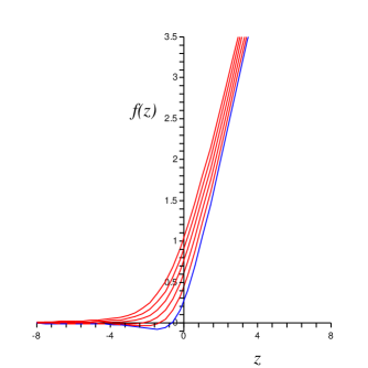
Figure 1: The non–perturbative solution for the function, $f(z)$, which contributes to the oriented sector of the model, for a range of positive values of $\Gamma$. The bottom curve is the $\Gamma=0$ case.

With each of these asymptotics comes two choices for $g(z)$, as solutions of $S=0$. For the large positive and negative $z$ directions, we have the choices, respectively:

$$g_{+,1}(z) = \pm 2\,\sqrt{z}+{\frac{\nu\,\left(\pm 3\,\Gamma-2\right)}{2z}}-{\frac{{\nu}^{2}\left(\pm 21\,{\Gamma}^{2}-36\,\Gamma\pm 20\right)}{16{z}^{5/2}}}+\cdots$$

$$g_{-,1}(z) = \pm i\sqrt{2}\sqrt{z}-{\frac{\nu}{z}}\mp{\frac{i\sqrt{2}{\nu}^{2}\left(12\,{\Gamma}^{2}-13\right)}{8{z}^{5/2}}}-{\frac{3{\nu}^{3}\left(12\,{\Gamma}^{2}-13\right)}{4{z}^{4}}}+\cdots$$ (34)

and we can also have third and fourth solutions that satisfy (32) but not (30):

$$g_{+,2}(z) = -{\frac{\nu}{z}}+{\frac{9{\nu}^{2}\Gamma}{4{z}^{5/2}}}-{\frac{15{\nu}^{3}\left(3\,{\Gamma}^{2}+2\right)}{8{z}^{4}}}+\cdots$$

$$g_{-,2}(z) = -{\frac{\nu}{z}}-{\frac{3{\nu}^{3}\left(12\,{\Gamma}^{2}-13\right)}{4{z}^{4}}}-{\frac{3{\nu}^{5}\left(336\,{\Gamma}^{4}-3384\,{\Gamma}^{2}+3085\right)}{16{z}^{7}}}+\cdots$$ (35)

An examination of the positive $z$ regime for the first case ($g_{+,1}$) shows (after integrating once and dividing by $\nu$) an expansion in $g_{s}$ again. It is clear that the first two terms are the contributions of $\IR{\rm P}^{2}$, the Möbius strip, and the Klein bottle, respectively. The diagrams come with a factor $g_{s}^{2h+b+c-2}\Gamma^{b}$ where $c$ is the number of crosscaps. In the negative $z$ regime we have an interpretation with just R–R fluxes again, the first term being $\IR{\rm P}^{2}$ and the next the Klein bottle. The next has contributions from closed surfaces with the following: $c=1,h=0$ and a flux insertion; $c=3,h=0$; $c=1,h=1$.

For the second case, there is again a surface interpretation consistent with there being D–branes in the positive $z$ regime, and fluxes in the negative $z$ regime. However, there are missing orders that deserve some explanation, which is perhaps to be found in a study of the continuum theory.

Plots of the non–perturbative completions of these two cases are given in figure 2.

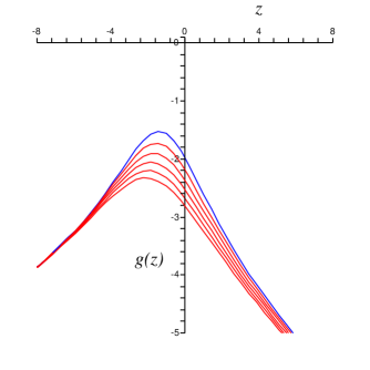
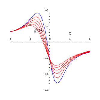
Figure 2: Two non–perturbative solutions for the function $g(z)$ which contributes to the unoriented sector of the model, for a range of positive values of $\Gamma$. In both cases the top curve is the $\Gamma=0$ case.

As in the case of the $[P,Q]=1$ formulation, it is tempting to speculate that all of these perturbative expansions for $g(z)$ are on equal footing; that is, they are equally valid in non-orientable string theory. Whether or not all these models stem from matrix models is also a question worth investigating.

Having arrived at the case $C_{0}=-1/4$, it is natural to wonder whether the other choices for $C_{0}$ are physical as well. After a little algebra, we find that we can rewrite equation (27) as the following:

$$S^{{}^{\prime}}+gS=2\nu\left(C_{0}+\frac{1}{4}\right)\equiv\nu G\ ,$$ (36)

where we have defined the constant $G$ for later convenience. The case before was $G=0$. To what do other values of $G$ correspond? The case of $C_{0}=0$ ($G=1/2$), which corresponds to the $\tilde{P}$ operator originally defined without the shift, gives the following expansions for $g$ (again two choices in each regime). For large positive $z$ we have:

$$g_{+,1}(z) = \pm 2\,\sqrt{z}+{\frac{3\nu\,\left(\pm 2\,\Gamma-1\right)}{4z}}-{\frac{{\nu}^{2}\left(\pm 84\,{\Gamma}^{2}-120\,\Gamma\pm 47\right)}{64{z}^{5/2}}}+\cdots$$

$$g_{+,2}(z) = -{\frac{3\nu}{2z}}+{\frac{3{\nu}^{2}\Gamma}{{z}^{5/2}}}-{\frac{3{\nu}^{3}\left(76\,{\Gamma}^{2}+77\right)}{32{z}^{4}}}+\cdots$$ (37)

while for the large negative $z$ regime we have:

$$g_{-,1}(z) = \pm i\sqrt{2}\sqrt{z}-{\frac{3\nu}{2z}}\mp{\frac{i\sqrt{2}{\nu}^{2}\left(24\,{\Gamma}^{2}-47\right)}{16{z}^{5/2}}}-{\frac{21{\nu}^{3}\left(8\,{\Gamma}^{2}-17\right)}{16{z}^{4}}}+\cdots$$

$$g_{-,2}(z) = -{\frac{3{\nu}^{3}\left(4\,{\Gamma}^{2}-1\right)}{2{z}^{4}}}-{\frac{6{\nu}^{5}\left(8\,{\Gamma}^{4}-54\,{\Gamma}^{2}+13\right)}{{z}^{7}}}+\cdots$$ (38)

Again, a surface interpretation can be given along the lines of those discussed below equations (34) and (35).

Leaving $G$ as a parameter in the solutions (rather analogous to $\Gamma$, which controls the number of background D–branes or R–R fluxes), these equations yield the following solutions for $g(x)$:

$$g_{+,1}(z) = \pm 2\,\sqrt{z}+{\frac{\nu\,\left(\pm 3\,\Gamma-2+G\right)}{2z}}-{\frac{{\nu}^{2}\left(\pm 21\,{\Gamma}^{2}+12\Gamma(G-3)\pm 3\,{G}^{2}\mp 18\,G\pm 20\right)}{16{z}^{5/2}}}+\cdots$$

$$g_{-,1}(z) = \pm i\sqrt{2}\sqrt{z}-{\frac{\nu\,\left(G+1\right)}{z}}\mp{\frac{i\sqrt{2}{\nu}^{2}\left(12\,{\Gamma}^{2}-6\,{G}^{2}-18\,G-13\right)}{8{z}^{5/2}}}+\cdots$$

$$g_{+,2}(z) = -{\frac{\nu\,\left(G+1\right)}{z}}+{\frac{3{\nu}^{2}\Gamma\,\left(2\,G+3\right)}{4{z}^{5/2}}}-{\frac{{\nu}^{3}\left(3{\Gamma}^{2}(8G+15)+2{G}^{2}(G+9)+46\,G+30\right)}{8{z}^{4}}}+\cdots$$

$$g_{-,2}(z) = {\frac{\nu\,\left(2\,G-1\right)}{z}}+{\frac{{\nu}^{3}\left(24\,{\Gamma}^{2}G-36\,{\Gamma}^{2}-16\,{G}^{3}+72\,{G}^{2}-98\,G+39\right)}{4{z}^{4}}}+\cdots$$ (39)

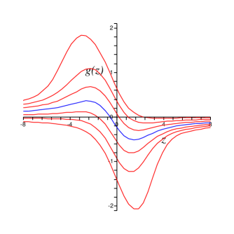
Figure 3: The non–perturbative solution for the function $g(z)$ which contributes to the unoriented sector of the model, for a range of values of $G$. The middle curve is the case of $G=0$.

These solutions interpolate between those displayed earlier for the cases $G=0$ and $G=1/2$. Figure 3 shows some sample plots of the full non–perturbative $g(z)$ for varying values of $G$. Upon examination of the expansions, it is tempting to interpret $G$ as a parameter controlling some aspect of the background, which is present only for the unoriented case. One possibility is that it incorporates the presence of some number, $G$, of a new type of D–brane that is present only in non–orientable diagrams (since it does not appear in the contributions from oriented surfaces). A candidate such brane could be one which is forced to remain stuck at (the analogue of) orientifold planes, a sort of fractional brane. This deserves further investigation. It is the case $G=0$ that has a known matrix model interpretation (by virtue of the map to self–dual unitary matrix models discussed earlier), and this would correspond to having such branes absent.

A possible clue to the nature of $G$ might be found in an examination of the instanton corrections to the expansions (terms exponentially small for small $g_{s}$), which often have an interpretation as D–branes in the theory[24, 25]. Some standard computations reveal that there are a number of instantons associated with each solution. These have actions (D–brane tensions) given by:

$$f_{+}:\quad\frac{4}{3}\frac{1}{g_{s}}\ ;\quad g_{+,1}:\quad\frac{4}{3}\frac{1}{g_{s}}\quad\mathrm{or}\quad\frac{2}{3}\frac{1}{g_{s}}\ ;\quad g_{+,2}:\quad\frac{2}{3}\frac{1}{g_{s}}\ ;\quad g_{+}:\quad\frac{2}{3}\frac{1}{g_{s}}\ .$$ (40)

In each case, the positive $z$ instanton has a negative $z$ counterpart which has an action precisely $1/\sqrt{2}$ times smaller. Here, the solution $g_{+}$ is the one obtained directly from the equation $S=0$. In each perturbative regime it appears that the tension of the unoriented expansion instantons takes one of two values: the same value associated to the oriented instanton; and half the value associated to the oriented instanton. It is therefore possible that this second unoriented instanton is the extra D–brane that is in the background, whose number is measured by $G$. This needs further work to properly establish however; but our picture is suggestive, if somewhat speculative.

The functions which give rise to $f$ and $g$ in the matrix model arise from orthogonal polynomial coefficients that come from effectively splitting the eigenvalues $\lambda_{i}$ of the matrices into the ones with even labels ($\lambda_{2j}$) and the ones with odd labels ($\lambda_{2j+1}$), respectively. The physics that arises from quantities controlled by $f$ are known to have an interpretation in terms of an eigenvalue distribution, the properties of which in the scaling limit can be interpreted in terms of background D–branes. In fact there is a direct map between the function $f$ and the eigenvalue distribution which can be studied on the sphere using an integral representation[26], or in terms of the resolvent of the operator $Q$[27]. The latter is particularly useful for going beyond the sphere and incorporating the effects of $\Gamma$ in the background, as recently shown in ref.[16]. It is natural to wonder if there is an effective eigenvalue distribution associated to the function $g$ that controls the physics of the unoriented sector. The instantons we computed above would have a natural home there in terms of the value of an effective potential at an extremum, and may correspond to a new type of D–brane. It seems likely (since $g$ arises as part of the operator $\tilde{P}$ which is made of a fractional power of $Q$) that there is some natural geometrical information to be extracted from $g$ analogous to an eigenvalue distribution and its effective potential. This is worth exploring.

Finally, it is known[28, 16] that the introduction of $\Gamma$ D–branes (or R–R flux units) into a closed minimal string background can be performed very elegantly in the language of the underlying twisted boson ($\varphi$, which is related to the loop operator and the resolvent) by simply acting with a vertex operator $V=:\exp(-\Gamma\varphi/\sqrt{2}):$ It would be interesting to see how the unoriented theory is described in this framework. Perhaps the role of $G$ may be best uncovered in this context.

Acknowlegements: JEC is supported by an EPSRC studentship, and also thanks the University of Southern California’s Department of Physics and Astronomy for hospitality.

References

- [1] R. C. Myers and V. Periwal, “Exact Solution Of Critical Selfdual Unitary Matrix Models,” Phys. Rev. Lett. 65 (1990) 1088–1091.
- [2] E. Brezin and V. A. Kazakov, “Exactly Solvable Field Theories Of Closed Strings,” Phys. Lett. B236 (1990) 144–150.
- [3] M. R. Douglas and S. H. Shenker, “Strings In Less Than One-Dimension,” Nucl. Phys. B335 (1990) 635.
- [4] D. J. Gross and A. A. Migdal, “Nonperturbative Two-Dimensional Quantum Gravity,” Phys. Rev. Lett. 64 (1990) 127.
- [5] E. Brezin and H. Neuberger, “Large N Scaling Limits Of Symmetric Matrix Models As Systems Of Fluctuating Unoriented Surfaces,” Phys. Rev. Lett. 65 (1990) 2098–2101.
- [6] G. R. Harris and E. J. Martinec, “Unoriented Strings and Matrix Ensembles,” Phys. Lett. B245 (1990) 384–392.
- [7] E. Brezin and H. Neuberger, “Multicritical points of unoriented random surfaces,” Nucl. Phys. B350 (1991) 513–553.
- [8] R. C. Myers and V. Periwal, “The Orientability Of Random Surfaces,” Phys. Rev. D42 (1990) 3600–3603.
- [9] V. Periwal and D. Shevitz, “Unitary Matrix Models As Exactly Solvable String Theories,” Phys. Rev. Lett. 64 (1990) 1326.
- [10] V. Periwal and D. Shevitz, “Exactly Solvable Unitary Matrix Models: Multicritical Potentials And Correlations,” Nucl. Phys. B344 (1990) 731–746.
- [11] I. R. Klebanov, J. Maldacena, and N. Seiberg, “Unitary and complex matrix models as 1-d type 0 strings,” hep-th/0309168.
- [12] S. Dalley, C. V. Johnson, and T. Morris, “Multicritical complex matrix models and nonperturbative 2-D quantum gravity,” Nucl. Phys. B368 (1992) 625–654.
- [13] S. Dalley, C. V. Johnson, and T. Morris, “Nonperturbative two-dimensional quantum gravity,” Nucl. Phys. B368 (1992) 655–670.
- [14] S. Dalley, C. V. Johnson, T. R. Morris, and A. Watterstam, “Unitary matrix models and 2-D quantum gravity,” Mod. Phys. Lett. A7 (1992) 2753–2762, hep-th/9206060.
- [15] T. R. Morris, “Checkered surfaces and complex matrices,” Nucl. Phys. B356 (1991) 703–728.
- [16] C. V. Johnson, “Tachyon condensation, open-closed duality, resolvents, and minimal bosonic and type 0 strings,” hep-th/0408049.
- [17] M. R. Douglas, “Strings In Less Than One-Dimension And The Generalized K-D- V Hierarchies,” Phys. Lett. B238 (1990) 176.
- [18] I. M. Gel’fand and L. A. Dikii, “Asymptotic behavior of the resolvent of Sturm-Liouville equations and the algebra of the Korteweg-De Vries equations,” Russ. Math. Surveys 30 (1975) 77–113.
- [19] V. G. Drinfeld and V. V. Sokolov, “Lie algebras and equations of Korteweg-de Vries type,” J. Sov. Math. 30 (1984) 1975–2036.
- [20] Y. Hikida, “Liouville field theory on a unoriented surface,” JHEP 05 (2003) 002, hep-th/0210305.
- [21] Y. Nakayama, “Tadpole cancellation in unoriented Liouville theory,” JHEP 11 (2003) 017, hep-th/0309063.
- [22] J. Gomis and A. Kapustin, “Two-dimensional unoriented strings and matrix models,” JHEP 06 (2004) 002, hep-th/0310195.
- [23] O. Bergman and S. Hirano, “The cap in the hat: Unoriented 2D strings and matrix(- vector) models,” JHEP 01 (2004) 043, hep-th/0311068.
- [24] S. H. Shenker, “The Strength of nonperturbative effects in string theory,”. Presented at the Cargese Workshop on Random Surfaces, Quantum Gravity and Strings, Cargese, France, May 28 - Jun 1, 1990.
- [25] J. McGreevy and H. Verlinde, “Strings from tachyons: The c = 1 matrix reloated,” hep-th/0304224.
- [26] D. Bessis, C. Itzykson, and J. B. Zuber, “Quantum field theory techniques in graphical enumeration,” Adv. Appl. Math. 1 (1980) 109–157.
- [27] F. David, “Loop Equations And Nonperturbative Effects In Two- Dimensional Quantum Gravity,” Mod. Phys. Lett. A5 (1990) 1019–1030.
- [28] C. V. Johnson, “On integrable open string theory,” Nucl. Phys. B414 (1994) 239–266, hep-th/9301112.