ITP-UU-04/17
SPIN-04/10
hep-th/0408148

MINIMAL STRINGS FOR BARYONS

Astract
A simple model is discussed in which baryons are represented as pieces of open string connected at one common point. There are two surprises: one is that, in the conformal gauge, the relative lengths of the three arms cannot be kept constant, but are dynamical variables of the theory. The second surprise (as reported earlier by Sharov) is that, in the classical limit, the state with the three arms of length not equal to zero is unstable against collapse of one of the arms. After collapse, an arm cannot bounce back into existence. The implications of this finding are briefly discussed.

1 Introduction

Mesons appear to be well approximated by an effective string model in four dimensions, even if anomalies and lack of super-symmetry cause the spectrum of quantum states to violate unitarity to some extent. Presumably this is because there are no difficulties with classical (open or closed) strings in any number of dimensions, without any super-symmetry. String theory can simply be seen as a crude approximation for mesons, and as such it works reasonably well, although some observed bending of the Regge trajectories at low energies is difficult to reproduce in attempts at an improved treatment of the quantization in such a regime.

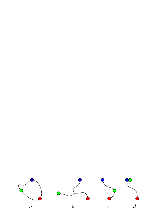
Figure 1: Four possible string models for baryons. $a)$ Three fermions on a closed string; $b)$ Our starting point: quarks attached by a single string; $c)$ After collapse of one arm; $d)$ With two quarks in a $\overline{3}$ bound state.

It would be very desirable to have an improved effective string model for QCD even if no refuge can be taken into any supersymmetric deformations of the theory[1]. Such a string model should explain the approximately linear Regge trajectories, and if we can refine it, one might imagine using it as an alternative method to compute spectra and transition amplitudes in mesons and baryons. Ideally, a string model would not serve as a replacement of QCD, but as an elegant computational approach.

The Regge trajectories for baryons seem to have the same slope as the mesonic ones. This can easily be explained if we assume baryons to consist of open strings that tend to have quarks at one end and diquarks at the other. The question asked in this short note is how a classical string model for baryons should be handled[2][3]. In the literature, there appears to be a preference for the $\Delta$ model[4], consisting of a closed string with three fermion-like objects attached to it, see Fig. 1$a$. As closed strings can be handled using existing techniques, this is a natual thing to try.

However, from a physical point of view, the Y configuration, sketched in Fig. 1$b$ appears to be a better representation of the baryons. After all, given three quarks at fixed positions, the Y shape takes less energy. Furthermore, if two of these quarks stay close together, they behave as a diquark and the Regge spectrum (with the same slope as the mesons) would be readily explained. However, there turns out to be a good reason why the Y shape is dismissed[6]; we will discuss this, and then ask again whether “$\Delta$” is to be preferred.

We considered the exercise of solving the classical string equations for this configuration. After we did this exercise, we found that it has been discussed already by Sharov[5]. The question will be whether we agree with his conclusions.

2 The three arms

The three arms are described by the coordinate functions $X^{\mu,i}(\sigma,\,\tau)$, where the index $i$ is a label for the arms: $i=1,2,$ or $3$. At the points $\sigma=0$, the three arms are connected:

$$X^{\mu,1}(0,\,\tau)=X^{\mu,2}(0,\,\tau)=X^{\mu,3}(0,\,\tau)\ .$$ (2.1)

$\sigma$ is a coordinate along the three arms. It takes values on the segment $[\,0,\,L^{i}(\tau)\,]$, where as yet we keep the lengths $L^{i}(\tau)$ unspecified.

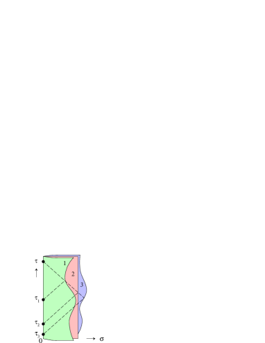
Figure 2: The three world sheets. Their relative lengths are dynamical variables. One of the three may be kept fixed. Dashed lines: bouncing waves have differing arrival times.

The Nambu action is

$$S=-\sum_{i=1}^{3}\int{\rm d}\tau\int_{0}^{L^{i}(\tau)}{\rm d}\sigma\,\sqrt{(\partial_{\sigma}X^{\mu,i}\cdot\partial_{\tau}X^{\mu,i})^{2}-(\partial_{\sigma}X^{\mu,i})^{2}(\partial_{\tau}X^{\lambda,i})^{2}}\,\Big{)}\ .$$ (2.2)

Here, as in the expressions that follow, we assume the usual summation convention for the Lorentz indices $\mu,\ \lambda,\ \dots$, but not for the branch indices $i$, where summation, if intended, will always be indicated explicitly. For simplicity, the masses of the quarks at the end points are neglected.

Assuming, in each of the three arms, the classical gauge condition

$$\partial_{\sigma}X^{\mu,i}\cdot\partial_{\tau}X^{\mu,i}=0\ ;$$ (2.3)

$$(\partial_{\sigma}X^{\mu,i})^{2}=-(\partial_{\tau}X^{\mu,i})^{2}\ ,$$ (2.4)

Eq. (2.2) takes the form

$$S=\sum_{i=1}^{3}\int{\rm d}\tau\int_{0}^{L^{i}(\tau)}{\rm d}\sigma\Big{(}{\textstyle{1\over 2}}(\partial_{\tau}X^{\mu,i})^{2}-{\textstyle{1\over 2}}(\partial_{\sigma}X^{\mu,i})^{2}\Big{)}\ .$$ (2.5)

3 Boundary conditions

The boundary condition at the origin can be enforced by two Lagrange multipliers: we add to the action (2.5)

$$\int{\rm d}\tau(\lambda_{1}^{\mu}(\tau)(X^{\mu,1}(0,\tau)-X^{\mu,3}(0,\tau))+\lambda_{2}^{\mu}(\tau)(X^{\mu,2}(0,\tau)-X^{\mu,3}(0,\tau))\ .$$ (3.1)

Now, considering an infinitesimal variation of $X^{\mu,i}(\sigma,\,\tau)$, we find

$$\delta S = \sum_{i}\bigg{(}\int{\rm d}\tau{\rm d}\sigma\,\delta X^{\mu,i}(\partial_{\sigma}^{2}-\partial_{\tau}^{2})X^{\mu,i}\ +$$ (3.2)

$$\int{\rm d}\tau\Big{(}\delta X^{\mu,i}(0,\,\tau)(\partial_{\sigma}X^{\mu,i}(0,\,\tau)+\lambda^{\mu}_{i})-\delta X^{\mu,i}(L^{i},\,\tau)\partial_{\sigma}X^{\mu,i}(L^{i}(\tau),\,\tau)\Big{)}\bigg{)}\ ,$$

where $\lambda_{3}=-\lambda_{1}-\lambda_{2}\,$. Thus, we see that the usual Neumann boundary condition holds at the three end points $\sigma=L^{i}$, while at the origin we have a Neumann boundary condition for the sum $\sum_{i=1}^{3}X^{\mu,i}$ and a Dirichlet condition for the differences:

$$\sigma=0\ : \partial_{\sigma}(X^{\mu,1}+X^{\mu,2}+X^{\mu,3})=0\ ;$$

$$X^{\mu,1}-X^{\mu,3}=X^{\mu,2}-X^{\mu,3}=0\ ,$$

$$\sigma=L^{i}(\tau)\ : \partial_{\sigma}X^{\mu,i}=0\ ,\quad\forall i\ .$$ (3.3)

4 Equations of motion

From Eq. (3.2), we read off the usual equations of motion implying that we have the sum of left- and right-going waves on all three branches:

$$X^{\mu,i}=X^{\mu,i}_{L}(\sigma+\tau)+X^{\mu,i}_{R}(\tau-\sigma)\ .$$ (4.1)

The boundary conditions (3.3) now read

$$X^{\mu,i}_{L}=X^{\mu,i}_{R}\qquad \mathrm{at} \ \sigma=L^{i}(\tau)\ ,\quad\mathrm{and}$$ (4.2)

$$\matrix{\partial_{\tau}X^{\mu,1}_{R}&=&\partial_{\tau}({\textstyle{2\over 3}}X_{L}^{\mu,2}+{\textstyle{2\over 3}}X_{L}^{\mu,3}-{\textstyle{1\over 3}}X_{L}^{\mu,1})\cr\partial_{\tau}X^{\mu,2}_{R}&=&\partial_{\tau}({\textstyle{2\over 3}}X_{L}^{\mu,3}+{\textstyle{2\over 3}}X_{L}^{\mu,1}-{\textstyle{1\over 3}}X_{L}^{\mu,2})\cr\partial_{\tau}X^{\mu,3}_{R}&=&\partial_{\tau}({\textstyle{2\over 3}}X_{L}^{\mu,1}+{\textstyle{2\over 3}}X_{L}^{\mu,2}-{\textstyle{1\over 3}}X_{L}^{\mu,3})}\ \Bigg{\}}\ \mathrm{at} \ \sigma=0\ .$$ (4.3)

In addition to these, we have the constraints (2.3) and (2.4), now taking the form

$$\sum_{\mu}(\partial_{\tau}X^{\mu,i}_{L})^{2}=\sum_{\mu}(\partial_{\tau}X^{\mu,i}_{R})^{2}=0\ .$$ (4.4)

These constraints should be compatible with the boundary conditions. The conditions at the three end points, Eqs. (4.2) give nothing extra, but the equations at the origin, Eqs. (4.3), require that, at that point, also

$$\partial_{\tau}X^{\mu,1}_{L}\,\partial_{\tau}X^{\mu,2}_{L}\ =\ \partial_{\tau}X^{\mu,2}_{L}\,\partial_{\tau}X^{\mu,3}_{L}\ =\ \partial_{\tau}X^{\mu,3}_{L}\,\partial_{\tau}X^{\mu,1}_{L}\ ,$$ (4.5)

and similarly for the right-going modes. From the point of view of causality, it might seem odd that there is a condition that the newly arriving modes should obey. However, it can easily be imposed by a relative rescaling of the coordinates $\,\sigma+\tau\,$ for the left-going modes in the three arms:

$$\partial_{\tau}X^{\mu,i}_{L}(\tau)\ =\ {{\rm d}\tau_{i}\over{\rm d}\tau}\ \partial_{\tau_{i}}X^{\mu,i}_{L}(\tau_{i})\ .$$ (4.6)

Indeed, as we shall now demonstrate, the requirement (4.5) fixes the functions $L^{i}(\tau)$.

Taking the fact that $X^{\mu,i}_{L}$ only depends on $\,\tau+\sigma\,$ and $X^{\mu,i}_{R}$ only on $\,\tau-\sigma\,$, the boundary condition (4.2) implies the existence of functions $\tau_{i}(\tau)<\tau$ such that

$$X^{\mu,i}_{L}(\tau)=X^{\mu,i}_{R}(\tau_{i})\ ,$$ (4.7)

where $\tau_{i}(\tau)$ are the solutions of

$$\tau-\tau_{i}\ =\ 2L^{i}(\tau^{\prime}_{i})\ ,\qquad\tau^{\prime}_{i}\equiv{\tau+\tau_{i}\over 2}\ .$$ (4.8)

These are just the three departure times, from the center, of each of the three returning waves, see Fig. 2. Now let

$$Q^{\mu,i}(\tau) \equiv {\partial X^{\mu,i}_{R}(\tau)\over\partial\tau}\ ;$$ (4.9)

$$R^{i}(\tau) \equiv -\,Q^{\mu,j}(\tau_{j})\,Q^{\mu,k}(\tau_{k})\ ,\qquad i,j,k=1,2,3\ \mathit{cyclic,}$$ (4.10)

(i,j,k being any even permutation of 1,2,3). The minus sign in Eq. (4.10) is chosen because $Q^{\mu,i}\,Q^{\mu,j}=\vec{Q}^{i}\cdot\vec{Q}^{j}-|Q^{i}||Q^{j}|\leq 0\,$, since $(Q^{\mu,i})^{2}=0\,$. Then, using (4.6), condition (4.5) implies

$${1\over R^{1}(\tau)}{{\rm d}\tau_{1}\over{\rm d}\tau}\ =\ {1\over R^{2}(\tau)}{{\rm d}\tau_{2}\over{\rm d}\tau}\ =\ {1\over R^{3}(\tau)}{{\rm d}\tau_{3}\over{\rm d}\tau}\ .$$ (4.11)

Together with a gauge condition for the overall time parameter $\tau$, for instance,

$${\textstyle{1\over 3}}\sum_{i}\tau_{i}=\tau-1\ ;\qquad\sum_{i}{{\rm d}\tau_{i}\over{\rm d}\tau}=3\ ,$$ (4.12)

these form complete differential equations that determine the functions $\tau_{i}(\tau)$, and thus also the functions $L^{i}(\tau)$, through Eqs. (4.8):

$${{\rm d}\tau_{i}\over{\rm d}\tau}={3R^{i}\over R^{1}+R^{2}+R^{3}}\ .$$ (4.13)

The complete update of the functions $Q^{\mu,i}(\tau)$ at the central point then reads:

$${Q^{\mu,i}}(\tau)\ =\ {1\over\sum R}\Big{(}2R^{j}(\tau)Q^{\mu,j}(\tau_{j})+2R^{k}(\tau)Q^{\mu,k}(\tau_{k})-R^{i}(\tau)Q^{\mu,i}(\tau_{i})\Big{)}\ ,$$

$$i,j,k=1,2,3\ \mathit{cyclic.}$$ (4.14)

Using Eqs. (4.10), one verifies that indeed the constraint $(Q^{\mu,i}(\tau))^{2}=0\,$ continues to be respected.

5 An instability

In the special case when all $R^{i}$ happen to be constant and equal, these equations can be solved. The three arms then have equal lengths, in the sense that waves running across the three arms bounce back in exactly the same time, which is constant. However, one readily convinces oneself that solutions with unequal arms should also exist. For instance, take an initial state described by functions $Q^{\mu,i}(\tau)$ consisting of superpositions of theta functions in $\tau$, such that the condition

$$\sum_{\mu}(Q^{\mu,i})^{2}=0$$ (5.1)

is always satisfied. One can then solve the equations stepwise for successive intervals in $\tau$.

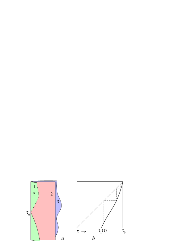
Figure 3: $a)$ A contracting arm. $b)$ Indefinite series of ‘updates’ of the data along the contracting arm, due to bouncing waves.

There is, however, a problem that needs to be addressed: what happens if one of the arms tends to vanish? This is for instance the case if, during some period, ${\rm d}\tau_{1}/{\rm d}\tau>1$ until $\tau-\tau_{1}\rightarrow 0$, see Fig. 3$a$. Do we need a new boundary condition addressing this situation? Indeed, it appears that, at least in the classical (unquantized) theory, an extra boundary condition will be needed. Our argument goes as follows.

If, at some value(s) of $\tau$, one arm length parameter, say $L^{1}(\tau)\,$, tends to zero, then there will be waves running up and down this arm increasingly frequently, see Fig. 3$b$. The values for $Q^{\mu,i}$ for the two long arms, $i=2,3$, will not vary rapidly during this small period (this is because these incoming waves were last updated at the times $\tau_{2}$ and $\tau_{3}$, both long before $\tau$). Let us make an educated guess about what will happen, by keeping these $Q$ vectors constant. In contrast, $Q^{\mu,1}(\tau)$ will be updated frequently, so, let us consider this sequence. We have

$${Q^{\mu,1}}(\tau) = {1\over\sum_{i}R^{i}}\Big{(}2R^{2}(\tau)Q^{\mu,2}(\tau_{2})+2R^{3}(\tau)Q^{\mu,3}(\tau_{3})-R^{1}(\tau)Q^{\mu,1}(\tau_{1})\Big{)}\ ,$$ (5.3)

$$Q^{\mu,2}(\tau_{2})\quad\mathrm{and}\quad Q^{\mu,3}(\tau_{3})\quad\mathit{constant}.$$

One finds that the parameters $R^{i}$ are updated as follows:

$$R^{1} \rightarrow R^{1}\equiv R\quad\mathrm{(constant)}\ ;$$

$$R^{2} \rightarrow {R^{1}\,R^{2}\over R^{1}+R^{2}+R^{3}}\ ;$$

$$R^{3} \rightarrow {R^{1}\,R^{3}\over R^{1}+R^{2}+R^{3}}\ .$$ (5.4)

This implies that $R^{2}$ and $R^{3}$ continue to decrease, until $R^{1}$ dominates. Thus,

$${{\rm d}\tau_{1}\over{\rm d}\tau}\rightarrow 3\ ,\qquad{{\rm d}\tau_{2}\over{\rm d}\tau}\rightarrow 0\ ,\qquad{{\rm d}\tau_{3}\over{\rm d}\tau}\rightarrow 0\ .$$ (5.5)

Since we started with $\tau_{1}<\tau$, we find that $\tau_{1}\rightarrow\tau\,$, rapidly. In fact, we found that, continuing along this line, assuming $Q^{\mu,2}$ and $Q^{\mu,3}$ to stay constant, the calculation can be done exactly. After $n$ iterations, the vector $Q^{\mu,1,\,(n)}$ becomes

$$Q^{\mu,1\,(n)}={1\over n}\Big{(}Q_{0}^{\mu}(-1)^{n}+\beta Q^{\mu,2}+(1-\beta)Q^{\mu,3}\Big{)}\ ,$$ (5.6)

where $Q_{0}^{\mu}$ is a fixed vector, and $\beta$ is a fixed coefficient, such that

$$Q_{0}^{\mu}\,Q^{\mu,2}=Q_{0}^{\mu}\,Q^{\mu,3}=0\ ;\qquad(Q_{0}^{\mu})^{2}=R\beta(1-\beta)\ ;\qquad Q^{\mu,2}\,Q^{\mu,3}=-R\ .$$ (5.7)

We also have

$$R^{2\,(n)}={\beta\over n}R\ ;\qquad R^{3\,(n)}={1-\beta\over n}R\ .$$ (5.8)

In fact, $Q_{0}^{\mu}$ and $\beta$ are only constant while following a bouncing wave, but they cannot be constant along the entire short arm. This is because of the alternating sign in Eq. (5.6). Since $Q_{0}^{\mu}$ is spacelike and orthogonal to $Q^{\mu,2}$ and $Q^{\mu,3}$, it must oscillate through zero. At such points, either $\beta$ or $1-\beta$ must have quadratic zeros. Typically, one of these will oscillate like $\sin^{2}(\pi\sigma/2L^{1})\,$. Thus, our solution consists of partly-periodic functions, in the sense that over periods lasting approximately $\ln 3$ in the parameter $\ln(\tau_{0}-\tau)$, the functions are updated using Eqs. (5.6), where the auxiliary functions (5.7) are exactly periodic.

We have no indication that small perturbances in the initial conditions will have drastic effects on these solutions, so that indeed generic solutions exist in which one arms rapidly shrinks to zero. What happens after such an event? At first sight, it seems reasonable to postulate some sort of bounce. By time-reversal symmetry, one might expect this arm to come back into existence. However, closer inspection makes such a ‘solution’ quite unlikely, or even impossible. Our observation is the following. Shortly before our shrinking event, the short arm has been violently oscillating, or rotating, around the central point. In doing so, the rapidly oscillating function $Q^{\mu,1}$ has been emitting high-frequency waves into the two long arms. These frequencies will always be much higher than the frequencies of oscillations entering from the long arms. The time-reversal of this configuration is hard to reconcile with causality requirements. Thus, the energy of the short arm has been dissipating in the form of high-frequency modes in the long arms, and the dissipated energy will be hard to recover.

6 Conclusion

We did not study possible quantization procedures for this model in any detail. Extreme non-linearity at the connection point probably makes this impossible. Qualitatively, as is well-known, one expects Regge trajectories that are similar — and have the same slope — as the mesonic ones, since at any given energy, the highest angular momentum states will be achieved when one arm vanishes. Now, in our analysis, we find that, as soon as a classical string picture is adopted for baryonic states, at least one of the three arms will soon disappear, shedding its energy into the excitation modes of the two other arms, see Fig. 1$c$.

This is somewhat counter-intuitive. One might have thought that equipartition should take place: all corners of phase space should eventually be occupied with equal probability. The answer to this is, of course, that phase space is infinite, so that equipartition is impossible. It is the old problem of statistical physics before the advent of Quantum Mechanics: there is an infinite amount of phase space in the high frequency domain. Since physical baryons are quantum mechanical objects, we expect an effective cut-off at high frequencies, simply because of energy quantization. This does mean, however, that in the high energy domain, the majority of baryonic states will have these high-energy modes excited. If, due to some electro-weak interaction, or possibly due to a gluon hitting a quark, a baryonic state is created with three quarks energetically moving in different directions, we expect first the Y shape to form, but then the most likely baryonic excitation that is reached is one with a single open string connecting the three quarks.

We found that the classically stable configuration has a single open string with two quarks at the end points and one quark moving around on the string. However, because of an attraction between two quarks into a $\overline{3}$ bound state (as opposed to the 6), one expects quantum effects eventually to favor the configuration of one quark at one end and a di-quark at the other end of a single open string, see Fig. 1$d$. I still do not see a strong case in favor of the $\Delta$ configuration. The latter seems to be closer related to a baryon-glueball bound state that will probably have a rather low production cross section.

Finally, Y shaped string configurations have also emerged in string theory[7], but only by viewing the connection point as a $D$-brane, which as such must be handled in the classical approximation, so that most of the mass of the system is concentrated there. The dynamical properies of such configurations will again be different from what we studied here.

References

- [1] A.A. Polyakov, A Few Projects in String Theory, hep-th/9304146, Chapter 8.
- [2] X. Artru, Nuc. Phys. B85 (1975) 442.
- [3] G.S. Sharov, Four Various String Baryon Models and Regge Trajectories, hep-ph/9809465.
- [4] G.S. Sharov, String baryon model “triangle”: hypocycloidal solutions, hep-th/9808099.
- [5] G.S. Sharov, Instability of Classic Rotational Motion for Three-String Baryon Model, hep-ph/0001154
- [6] G.S. Sharov, Quasirotational Motions and Stability Problem in Dynamics of String Hadron Models, hep-ph/0004003
- [7] E. Witten, Baryons and Branes in Anti de Sitter Space, hep-th/9805112.