UPR-1086-T
Lectures on D-branes, Gauge Theories and Calabi-Yau Singularities

These lectures, given at the Chinese Academy of Sciences for the BeiJing/HangZhou International Summer School in Mathematical Physics, are intended to introduce, to the beginning student in string theory and mathematical physics, aspects of the rich and beautiful subject of D-brane gauge theories constructed from local Calabi-Yau spaces. Topics such as orbifolds, toric singularities, del Pezzo surfaces as well as chaotic duality will be covered.

1 Introduction

“For any thing so overdone is from the purpose of playing, whose end, both at the first and now, was and is, to hold, as ’twere, the mirror up to Nature.” And thus The Bard has so well summed up (Hamlet, III.ii.5) a sometime too blunted purpose of String Theory, that she, whilst enjoying her own Beauty, should not forget to hold her mirror up to Nature and that her purpose, as a handmaid to Natural Philosophy, is to reflect a Greater Beauty in Nature’s design. These lectures, as I was asked, are intended to address an audience equally partitioned between students of mathematics and physics. I will attempt to convey the little I know on some aspects of the deep and elegant interactions between physics and mathematics within the subject of gauge theories on D-brane world-volumes arising from compactifications on Calabi-Yau spaces; I will try to inspire the physicist with the astounding mathematical structures and to hearten the mathematicians with the insightful physical computations, but I shall always emphasise an underlying theme of Nature, that this subject of studying gauge theories arising from string compactifications is, sicut erat in principio, et nunc, et semper, motivated by the pressing need of uniquely obtaining the Standard Model from string theory.

The lectures are entitled D-branes, gauge theories and Calabi-Yau singularities. I must motivate the audience as to why we wish to study these concepts. First, let me address the physicists. The gauge theory aspect is clear. Depending on the particulars, string theory possesses, ab initio, a plethora of gauge symmetries, from the Chan-Paton factors of the open string to the $E_{8}\times E_{8}$ or $Spin(32)/\mathbb{Z}_{2}$ groups of the heterotic string. Our observable world is a four-dimensional gauge theory with the group $SU(3)\times SU(2)\times U(1)$ with possible but not-yet-observed supersymmetry (SUSY); methods must be devised to reduce the gauge group of string theory thereto.

Of course, of equal pertinence is the need to reduce dimensionality. The ten dimensions of string theory (or the eleven dimensions of the parent M-theory) can only have four directions in the macroscopic scale. The traditional approach has been compactification and this is where Calabi-Yau spaces enter the arena. We will impose ${\mathcal{N}}=1$ supersymmetry in four dimensions. This imposition is completely independent of string theory. Many phenomenologists find the possibility of ${\mathcal{N}}=1$ SUSY at the electroweak scale appealing because, amongst other virtues, it helps to provide a natural solution to the hierarchy problem: the amount of fine-tuning needed to make the Higgs mass at the electro-weak scale. The six-dimensional space for compactification is constrained by this imposition of low-energy supersymmetry to be a Calabi-Yau (complex) threefold.

Why, then, D-branes? As it is by now well-known, string theory contains one of the most amazing dualities, viz., Maldacena’s AdS/CFT duality, relating bulk string theory with a holographic boundary gauge theory. The root of this correspondence is the open/closed string duality wherein the open strings engender the gauge theory while the closed strings beget gravity. The boundary conditions for the open strings are D-branes, which are dynamical objects in their own right. Therefore, our stringy compactification necessarily includes the subject of D-branes probing Calabi-Yau spaces.

The paradigm we will adopt is a “brane-world” one. We let our world be a slice in the ten-dimensions of the Type II superstring. In other words, we let the four dimensional world-volume of the D3-brane carry the requisite gauge theory, while the bulk contains gravity. Therefore, as far as the brane is concerned, the six transverse Calabi-Yau dimensions can be modeled as non-compact (affine) varieties. This “compactification” by non-compact Calabi-Yau threefolds greatly simplifies matters for us. Indeed, an affine variety that locally models a Calabi-Yau space is far easier to handle than the compact manifold sewn together by local patches.

The draw-back, or rather, the boon - for a myriad of rich phenomena germinates - is the obvious fact that the only smooth local Calabi-Yau threefold is $\mathbb{C}^{3}$. We are thus inevitably lead to the study of singular Calabi-Yau varieties. This is reminiscent of the fact that in standard heterotic phenomenology it is the singular points in the moduli space of compactifications that are of particular interest. The qualifiers local, non-compact, affine and singular will thus be used interchangeably henceforth. In summary then, our D-brane resides transversely to a singular non-compact Calabi-Yau threefold. On the D-brane world-volume we will live and observe some low-energy effective theory of an ${\mathcal{N}}=1$ extension of the Standard Model.

Now, let me turn to address the mathematicians. Of course, the astonishing phenomenon of mirror symmetry for Calabi-Yau threefolds has become a favoured theme in modern geometry. Mirror pairs often involve singular manifolds and in particular, quotients. Indeed, the local mirror programme has been extensively used to compute topological string amplitudes and, hence, Gromov-Witten invariants for counting curves. Thus far, affine Calabi-Yau singularities used in local mirrors have been predominantly toric varieties such as the conifold and cones over del Pezzo surfaces. These, together with above-mentioned quotient spaces, shall also constitute the primary examples which we will study.

The resolution of singularities has been a classic and ongoing subject. Ever since McKay’s discovery of the correspondence between the finite discrete subgroups of $SU(2)$ and affine simply-laced Lie algebras, geometers have been attempting to explain this correspondence using resolutions of $\mathbb{C}^{2}$ quotients and to extend it to higher dimensions. Now, we have a new tool.

String theory, being a theory of extended objects, is well-defined on such singularities. As far back as the 1980’s, Dixon, Harvey, Vafa and Witten had realised that closed strings can propagate unhindered on orbifolds. In addition, they made a simple prediction for the Euler character of the orbifold in terms of the resolved space, prompting the study by mathematicians such as V. Batyrev, S. S. Roan and Y. B. Ruan.

The open-string sector of the story, initiated by the investigations of Douglas and Moore, is concerned with D-brane resolutions of singularities. Quiver theories that arise have been used by Ito, Nakajima, Reid, Sardo-Infirri et al. to understand the essence of the McKay correspondence. Recent advances, notably by Bridgeland, King and Reid, have understood and re-casted it as an auto-equivalence in the bounded derived category of coherent sheafs on the resolved space. Indeed, this is closely related to the physicist’s understanding of D-branes precisely as objects in the derived category.

Realising branes as such objects, or more loosely, as supports of vector bundles (sheafs) is the mathematician’s version of brane-worlds. With the help of the works of Donaldson, Uhlenbeck and Yau, wherein solving for the phenomenological constraints of super-Yang-Mills theory in four dimensions during compactification has been reduced to constructing polystable vector bundles, one could move from the differential to the nominally simpler algebraic category. Thus, gauge theory on branes are intimately related to algebraic constructions of stable bundles.

In particular, D-brane gauge theories manifest as a natural description of symplectic quotients and their resolutions in geometric invariant theory. Witten’s gauged linear sigma model description, later utilised by Aspinwall, Greene, Morrison et al. as a method of finding the vacuum of the gauge theory, provided a novel perspective on symplectic quotients, especially toric varieties. In summary then, our D-brane, together with the stable vector bundle (sheaf) supported thereupon, resolves the transverse Calabi-Yau singularity which is the vacuum for the gauge theory on the world-volume as a GIT quotient.

Hopefully, I have given ample reasons why both physicists and mathematicians alike should study D-brane gauge theories on singular Calabi-Yau spaces. The motivations are summarised in Figure 1. Without much ado, let me proceed to the lectures. The students can refer to [17] wherein most of the material in the first two lectures are expanded.

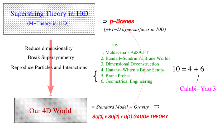
Figure 1: A pictorial representation of our motivations. We need to reduce the 10 dimensions of superstring theory with various gauge groups down to a 4 dimensional world with ${\mathcal{N}}=1$ supersymmetry and $SU(3)\times SU(2)\times U(1)$ gauge group with specific matter content and interactions. Various techniques have been adopted. The one we will study here is that of D3-branes probing a transverse Calabi-Yau threefold singularity.

2 Minute Waltz on the String

To set the arena let me very rapidly present to the neophytes, the necessary ingredients from type IIB superstring theory which will be used [1]. The section is hopefully to be perused in a single minute. The theory is a ten dimensional one with 32 super-charges and there is a spinor generator corresponding to the $2^{10/2}=32$ dimensional representation of the Clifford algebra. This is a theory of closed strings, i.e., mapping from $S^{1}$ to the Minkowski $\mathbb{R}^{1,9}$ spacetime. Bosonic particles are excitations on the world-sheet, which is here a cylinder, traced out by $S^{1}$ in spacetime. Fermionic particles also exist, as is required by supersymmetry. Indeed, spacetime supersymmetry is induced by the existence of worldsheet fermions the boundary conditions on which first gave the name type IIB.

By the closed/open duality inherent in string theory, that the existence of one necessitates that of the other (as the tree-level amplitude of the closed string is the vacuum loop of the open), we also have open strings in the theory. They must end on subspaces of $\mathbb{R}^{1,9}$. The subspaces which provide Dirichlet boundary conditions for the ends of the open strings are known as D-branes. We shall call one with a $p+1$-dimensional world-volume a Dp-brane. Pictorially, this is represented in Figure 2. Polchinski’s [2] realisation, that Dp-branes are dynamical objects carrying $p+1$-form charges, brought D-branes on an equal footing as the fundamental string. In type IIB, $p$ will take values of all odd integers from 1 to 10. For our purposes, we will henceforth take $p=3$, and our world will be $3+1$-dimensional, as it is so observed.

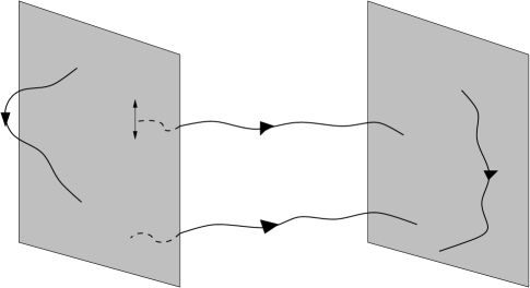
Figure 2: Open strings stretched between parallel D-branes. On the world-volume of each brane is a $U(1)$ gauge bundle. As the two coincide, the gauge group is enhanced to $U(2)$.

2.1 The D3-brane in $\mathbb{R}^{1,9}$

Now, open strings have in their spectrum, a massless vector particle, i.e., a $U(1)$ gauge field. Therefore, the D-brane must carry a $U(1)$ gauge connexion on its world-volume so as to accommodate the charge on the ends of the open string. It is in this sense that we consider the D-brane as supporting a $U(1)$ vector bundle (sheaf). When we place a stack of $n$ parallel D-branes coincident upon each other, we would naïvely expect a $U(1)^{n}$ gauge theory on the world volume. Instead, we have an enhancement to the non-Abelian group $U(n)$. As can be seen from Figure 2, this gauge enhancement is due to the open strings which are stretched between the parallel branes. The masses of these strings are proportional to the distance between the branes and thus as the brane become coincident, we have massless particles that are precisely the extra gauge fields.

2.2 D3-branes on Calabi-Yau threefolds

So far we have a ten dimensional theory of superstrings, and D-branes on which there could be an $U(n)$ gauge group. This, of course, is quite far from a Standard Model in four dimensions. We now follow the canonical practice of considering string theory not on $\mathbb{R}^{1,9}$ but on $\mathbb{R}^{1,4}\times M^{(6)}$ where $M^{(6)}$ is some internal manifold at the string scale, too small to be observed. This is known as compactification, an idea dating back to T. Kaluza and O. Klein in 1926. As mentioned earlier, we shall require that our $\mathbb{R}^{1,3}$ universe have ${\mathcal{N}}=1$ supersymmetry (which may be subsequently broken at a lower energy scale). This translates to the existence of covariantly constant spinors on $M^{(6)}$ that would function as the supersymmetric charge.

The solution for $M^{(6)}$ is that it is (1) compact, (2) complex (i.e., of dimension $3=6\div 2$), (3) Kähler (the metric $g_{\mu\bar{\nu}}$ should equal to $\partial_{\mu}\partial_{\bar{\nu}}K$ for some scalar $K$) and (4) has $SU(3)$ Holonomy. E. Calabi, an old gentleman of a distinguished bearing whose office is two floors up from mine, conjectured in 1954 that such manifolds should admit a unique Ricci-flat metric in each Kähler class. It was only until 1971 that this conjecture was proven by S.-T. Yau, who has been gracious to organise this summer school, by a tour de force differential analysis. In their honour, $M^{(6)}$ is called a Calabi-Yau threefold.

As far as our brane-world is concerned, we have four dimensional D3-branes in $\mathbb{R}^{1,4}\times M^{(6)}$ on which there is an $U(n)$ gauge group and transverse to which gravity propagates. We take the $\mathbb{R}^{1,4}$ to be precisely the world-volume of the brane and the transverse directions will be Calabi-Yau. In this scenario, the Calabi-Yau manifold is to be taken as non-compact, filling the remaining six dimensions. In other words, $M^{(6)}$ is an affine variety that locally models a Calabi-Yau threefold.

Indeed, if $M^{(6)}$ were smooth, then it can only be the trivial case of $\mathbb{C}^{3}$; we will address this case in the following section. Therefore, we are lead to $M^{(6)}$ being singular. We will see that it is exactly the singular structure of the geometry which aids us phenomenologically: it will break $U(n)$ into product gauge groups, it will reduce supersymmetry and it will yield particles that transform under the gauge factors. We remark that the general problem of D-branes on compact Calabi-Yau manifolds, instead of a mere affine patch, is an extremely difficult one and excellent reviews may be found in [71, 72]. One reason why we choose the brane-world paradigm wherein the transverse space can be taken as a non-compact local model, is that technically this is a much simpler problem.

A point, almost trivial, which I must emphasise, is that, as far as the transverse singularity is concerned, the D3-brane is a point. This obvious fact places a crucial relationship between the D3-brane world-volume theory and the Calabi-Yau singularity: that the latter should parametrise the former. That is, the classical vacuum of the gauge theory on the D3-brane should be, in explicit coördinates, the defining equation of $M^{(6)}$. I will re-iterate this point later.

For now, let us summarise the philosophy pictorially in Figure 3. We place a stack of $n$ D3-branes transverse to a Calabi-Yau threefold $M^{(6)}$, which, since it is singular, we will henceforth call $S$. The local model $S$ will afford some explicit description as an affine variety. The geometry of $S$ will project the $U(n)$ gauge theory to product gauge groups (ultimately that of the Standard Model). The singularities so far used have been orbifolds, toric singularities and cones over del Pezzo surfaces, the relations amongst which are drawn in the Venn diagram in the figure.

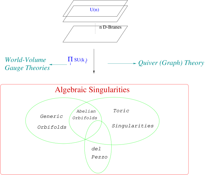
Figure 3: Our paradigm is to place a stack of $n$ parallel coincident D3-branes on an affine Calabi-Yau threefold singularity $S$. The geometry of $S$ will project the $U(n)$ gauge group on the branes to product gauge groups with bi-fundamental matter and interactions. The resulting theory is conveniently represented as a quiver diagram. Examples of $S$ thus far investigated have been orbifolds, toric singularities and cones over del Pezzo surfaces, as shewn in the Venn diagram.

3 The Simplest Case: $S=\mathbb{C}^{3}$

Let me begin with the simplest non-compact Calabi-Yau threefold. This is, of course, when $S$ is $\mathbb{C}^{3}$, which is trivially Ricci flat. Here, the D3-brane freely propagates in flat space. The world volume theory has a $U(n)$ gauge group as mentioned above. The presence of the brane breaks the $SO(1,9)$ Lorentz symmetry of $\mathbb{R}^{1,9}$, whereby breaking half of the supersymmetry and we are left with 16 supercharges. In four dimensions, this amount of supercharges corresponds to $16/2^{4/2}=4$ supersymmetry. We therefore have ${\mathcal{N}}=4$ superconformal (SCFT) $U(n)$ gauge theory on the world-volume.

This gauge theory, is the famous boundary SCFT for Maldacena’s Correspondence [3]. Of course, the D3-brane will warp the flat space metric to that of $AdS_{5}\times S^{5}$ and the bulk geometry is not strictly $\mathbb{C}^{3}$. However, as stated above, we are only concerned with the local gauge theory and not with gravitational back-reaction, therefore it suffices to consider $S$ as $\mathbb{C}^{3}$.

The matter content of the theory is as follows. There is a gauge field $A^{\mu}$ under the $U(n)$ group. Moreover, there is an $SU(4)$ R-symmetry inherent to the ${\mathcal{N}}=4$ SCFT which essentially is a rotation of the four supersymmetries. Of course, in the AdS/CFT picture, this $SU(4)\simeq SO(6)$ is the isometry group of the $S^{5}$ factor in $AdS_{5}\times S^{5}$. Under this R-symmetry, there are Weyl fermions $\Psi_{IJ}^{\bf{4}}$, $I,J=1,\ldots,n$, transforming as the ${\bf 4}$ of the $SU(4)$ and as adjoints under $U(n)$. The SUSY partners are bosonic fields $\Phi_{IJ}^{\bf{6}}$ under the ${\bf 6}$ of the $SU(4)$. The superpotential is uniquely determined by the matter. In terms of the three chiral superfields $C^{i}$, it is simply $W={\mathop{\rm Tr}}(C^{i}C^{j}C^{k})\epsilon_{ijk}$. For the mathematicians in the audience, we will consider $A^{\mu}$ as ${\rm Hom}(\mathbb{C}^{n},\mathbb{C}^{n})$, $\Psi_{IJ}^{\bf{4}}$ as ${\bf 4}\otimes{\rm Hom}(\mathbb{C}^{n},\mathbb{C}^{n})$, and $\Phi_{IJ}^{\bf{6}}$ as ${\bf 6}\otimes{\rm Hom}(\mathbb{C}^{n},\mathbb{C}^{n})$. What I have described above we shall call the “parent theory.” Her progeny will be the subject matter of these lectures.

4 Orbifolds and Quivers

The next best things to $\mathbb{C}^{3}$ are its quotients. This simple class of singularities is called orbifolds and has been studied as far back as the 1960’s by Satake et al. [4]. Here, I take $\mathbb{C}^{3}$ and quotient is by some discrete finite group $\Gamma$. The group action is

$$(\gamma\in\Gamma):(x,y,z)\rightarrow\gamma\cdot(x,y,z),$$ (4.1)

where the element $\gamma$ is written in explicit matrix representation and $(x,y,z)$ are the complex coördinates of $\mathbb{C}^{3}$. We see that the origin $(0,0,0)$ is a fixed point. Because of this fixed point, i.e., the action is not free, the quotient $\mathbb{C}^{3}/\Gamma$ consisting of equivalence class under the group action, is not a smooth manifold.

Certainly, $\Gamma$ cannot be arbitrary. In order that $S=\mathbb{C}^{3}/\Gamma$ be a Calabi-Yau singularity, it must admit a resolution to a smooth Calabi-Yau manifold $\tilde{S}$. This is known as a crepant resolution, i.e., for the map $f:\tilde{S}\rightarrow S$,

$$f^{*}K_{S}=K_{\tilde{S}}={\mathcal{O}}_{\tilde{S}},$$ (4.2)

where $K_{S}$ and $K_{\tilde{S}}$ are the canonical sheaves of $S$ and $\tilde{S}$ respectively and $K_{\tilde{S}}$ is trivial since $\tilde{S}$ is Calabi-Yau. The subject of crepant resolutions is one in its own right and the mathematicians in the audience are referred to, for example, [5, 6]. For our purposes I will take $\Gamma$ to be a discrete finite subgroup of $SU(3)$, i.e., the holonomy of $\tilde{S}$. This is not a sufficient condition for crepancy, but the techniques we introduce below work in general. For $\Gamma\subset SU(2)$, i.e., $S=\mathbb{C}\times\mathbb{C}^{2}/\Gamma$, however, they all have crepant resolutions and have a beautiful structure which we will present later. The case of $\Gamma\subset(SU(4)\simeq SO(6))$ is also possible [25] but we need to consider $S=\mathbb{R}^{6}/\Gamma$; this is, for now, of less interest to us because it is a real quotient and preserves no SUSY.

4.1 Projection to Daughter Theories

As initiated in the study of Douglas and Moore [7], with cases addressed by Johnson and Meyers [8], and the methodology formalised by Lawrence, Nekrasov and Vafa [9], let us now study what happens to the parent theory due to $S$. The prescription is straight-forward: we will use elements $\gamma$ to project out any states not invariant under $\Gamma$. That is, only $A^{\mu}$, $\Psi_{IJ}^{4}$ and $\Phi_{IJ}^{6}$ that satisfy

$$\gamma A^{\mu}\gamma^{-1}=A^{\mu},\quad\Psi_{IJ}^{4}=R(\gamma)\gamma\Psi^{4}_{IJ}\gamma^{-1},\quad\Phi_{IJ}^{6}=R(\gamma)\gamma\Phi^{6}_{IJ}\gamma^{-1}$$ (4.3)

remain in the spectrum. We have used $R(\gamma)$ for the matter fields since there should also be an extra induced action on the R-symmetry. Furthermore, the resulting SUSY is the commutant of $\Gamma$ in $SU(4)$. That is, the R-symmetry left untouched by $\Gamma$ will serve as the R-symmetry of the daughter theory.

More formally, in the notation of [9], let the irreducible representation of $\Gamma$ be $\left\{{\bf r}_{i}\right\}$ and decompose

$$\mathbb{C}^{n}\simeq\bigoplus\limits_{i}\mathbb{C}^{N_{i}}{\bf r}_{i}$$ (4.4)

for integer multiplicities $N_{i}$. Then, the resulting gauge group is given by the $\Gamma$-invariant part of the gauge group ${\rm Hom}\left(\mathbb{C}^{n},\mathbb{C}^{n}\right)$. That is,

$${\rm Hom}\left(\mathbb{C}^{n},\mathbb{C}^{n}\right)^{\Gamma}=\bigoplus_{i,j}\left(\mathbb{C}^{N_{i}}\otimes\mathbb{C}^{N_{j}*}\otimes{\bf r_{i}}\otimes{\bf r_{j}^{*}}\right)^{\Gamma}=\bigoplus\limits_{i}\mathbb{C}^{N_{i}}{\bf\otimes}\left(\mathbb{C}^{N_{i}}\right)^{*},$$ (4.5)

where we have used Schur’s Lemma that $({\bf r_{i}}\otimes{\bf r_{j}^{*}})^{\Gamma}=\delta_{ij}$ for irreducible representations $\left\{{\bf r}_{i}\right\}$. In other words, the daughter gauge group is $\prod\limits_{i}U(N_{i})$ with $N_{i}$ given in (4.4). It turns out that in the low energy effective theory the $U(1)$ factors decouple. Therefore, in fact, the resulting gauge group is $\prod\limits_{i}SU(N_{i})$.

Now, the matter fields $\Psi_{IJ}^{4}$ and $\Phi_{IJ}^{6}$ encounter a similar projection. For ${\cal R}={\bf 4}$ or 6, we have

$$\left({\cal R}\otimes{\rm Hom}\left(\mathbb{C}^{n},\mathbb{C}^{n}\right)\right)^{\Gamma} = \bigoplus_{i,j}({\cal R}\otimes\left(\mathbb{C}^{N_{i}}\otimes\mathbb{C}^{N_{j}*}\otimes{\bf r_{i}}\otimes{\bf r_{j}^{*}}\right))^{\Gamma}$$ (4.6)

$$= \bigoplus_{i,j}a_{ij}^{{\cal R}}\left(\mathbb{C}^{N_{i}}\otimes\mathbb{C}^{N_{j}*}\right),$$

where we have again made use of Schur’s Lemma and, in addition, the decomposition

$${\cal R}\otimes{\bf r}_{i}=\bigoplus\limits_{j}a_{ij}^{{\cal R}}{\bf r}_{j}$$. (4.7)

In other words, the matter fields become a total of $a_{ij}^{{\bf 4}}$ bi-fundamental fermions and $a_{ij}^{{\bf 6}}$ bi-fundamental bosons transforming as the $(N_{i},\bar{N}_{j})$ of $SU(N_{i})\times SU(N_{j})$ under the product gauge groups. To solve (4.7), one uses standard orthogonality conditions in character theory and obtain [18]

$$a_{ij}^{{\cal R}}=\frac{1}{g}\sum\limits_{\gamma=1}^{r}r_{\gamma}\chi_{\gamma}^{{\cal R}}\chi_{\gamma}^{(i)}\chi_{\gamma}^{(j)*},$$ (4.8)

where $g=\left|\Gamma\right|$ is the order of the group, $r_{\gamma}$ is the order of the conjugacy class containing $\gamma$ and $\chi_{\gamma}^{i}$ is the character of $\gamma$ in the $i$-th representation. We summarise the daughter theories below:

$$\begin{array}[]{|l|l|l|l|}\hline\cr&$Parent$&\stackrel{{\scriptstyle\Gamma}}{{\longrightarrow}}&$Orbifold Theory$\\ \hline\cr$SUSY$&{\cal N}=4&\leadsto&\begin{array}[]{l}{\cal N}=2,{\rm~{}for~{}}\Gamma\subset SU(2)\\ {\cal N}=1,{\rm~{}for~{}}\Gamma\subset SU(3)\\ {\cal N}=0,{\rm~{}for~{}}\Gamma\subset\{SU(4)\simeq SO(6)\}\\ \end{array}\\ \hline\cr\begin{array}[]{c}$Gauge$\\ $Group$\end{array}&U(n)&\leadsto&\prod\limits_{i}U(N_{i}),\qquad\sum\limits_{i}N_{i}{\rm dim}{\bf r}_{i}=n\\ \hline\cr$Fermion$&\Psi_{IJ}^{\bf{4}}&\leadsto&\Psi_{f_{ij}}^{ij}\\ $Boson$&\Phi_{IJ}^{\bf{6}}&\leadsto&\Phi_{f_{ij}}^{ij}\qquad\qquad{\cal R}\otimes{\bf r}_{i}=\bigoplus\limits_{j}a_{ij}^{{\cal R}}{\bf r}_{j}\\ \hline\cr\end{array}$$ (4.9)

for $I,J=1,...,n$ and $f_{ij}=1,...,a_{ij}^{{\cal R}={\bf 4},{\bf 6}}$.

4.2 Quivers

A convenient and visual representation of the resulting matter content in (4.9) is the so-called quiver diagram, originating from the German “Köcher” [24]. The rules are simple: it is a finite directed graph such that each node $i$ represents a gauge factor $SU(N_{i})$ and each arrow $i\rightarrow j$, a bi-fundamental field $(N_{i},\bar{N}_{j})$. The adjacency matrix $A$ of the graph is a $k\times k$ matrix with $k$ being the number of nodes (gauge factors) and encodes this information by having its entry $A_{ij}$ counting the number of arrows (bi-fundamentals) from $i$ to $j$. My discussing finite graphs at this point is hardly a digression. We will see next that the very usage of quiver is undoubtedly inspired by a remarkable correspondence.

4.3 The McKay Correspondence

Let us specify the discussions in (4.9) to the case of ${\mathcal{N}}=2$, i.e., to orbifolds of the type $\mathbb{C}^{3}/\Gamma\simeq\mathbb{C}\times\mathbb{C}^{2}/(\Gamma\subset SU(2))$. In 1884, F. Klein, in finding transcendental solutions to the quintic problem [11], classified the discrete finite subgroups of $SU(2)$. These are double covers of those of $SO(3)$, which simply constitute the symmetries of the perfectly regular shapes in $\mathbb{R}^{3}$, viz. the Platonic Solids. The groups fall into 2 infinite series, associated to the regular polygons, as well as 3 exceptionals, associated with the 5 regular polyhedra: the tetrahedron, the cube (and its dual tetrahedron) and the icosahedron (and its dual dodecahedron). The groups are

$$\begin{array}[]{|c|l|c|}\hline\cr\mbox{Group}&\mbox{Name}&\mbox{Order}\\ \hline\cr A_{n}\simeq\mathbb{Z}_{n+1}&\mbox{Cyclic}&n+1\\ \hline\cr D_{n}&\mbox{Binary Dihedral}&2n\\ \hline\cr E_{6}&\mbox{Binary Tetrahedral}&24\\ \hline\cr E_{7}&\mbox{Binary Octahedral (Cubic)}&48\\ \hline\cr E_{8}&\mbox{Binary Icosahedral (Dodecadedral)}&120\\ \hline\cr\end{array}$$ (4.10)

It was not until 1980, almost a full century later, that a remarkable correspondence between these groups and Lie algebras were realised by J. McKay [12], yes, the very McKay also responsible for initiating Moonshine. It has never ceased to astounded me, this uncanny ability of his to recognise, amidst a seeming cacophony of sounds, a single strain of melody. I first met John in Warwick I believe, me in my younger and even more ignorant days, him ruddy faced and a glass of wine in hand. Overcoming my initial trepidation by a few quick bites at my own sturdy drink - my liver being more lively at the time - I proceeded to him with reverence. But my intimidation was unwarranted and with paternal patience he explained at length his new conjectures regarding modular forms, sporadic groups and exceptional algebras, which, alas, due part to my own wanting of knowledge and part to the fine workings of the potent liquid upon my head, I only managed a vague glimpse, a fuller view of which only of late, fewer hair and dryer stomach, did I acquire in more conversations with him.

What McKay realised was that one can take the Clebsch-Gordan decomposition for ${\cal R}$, the fundamental 2 of $\Gamma\subset SU(2)$ and $\{{\bf r}_{i}\}$, the irreps. That is, one can take

$${\bf 2}\otimes{\bf r}_{i}=\bigoplus\limits_{j}a_{ij}^{{\bf 2}}{\bf r}_{j},$$ (4.11)

and treat $a_{ij}^{{\bf 2}}$ as the adjacency matrix of some finite graph. Then, the graphs are precisely the Dynkin diagrams of the affine simply-laced Lie algebras:

(4.12)

In other words, the McKay quiver for $\Gamma$ is in one-one correspondence with the affine ADE Lie algebras (the affine diagram adds one more node to the usual Dynkin diagram, here corresponding to the trivial representation) and the matrices $a_{ij}^{{\bf 2}}$ in (4.11) are precisely the Cartan matrices of the associated algebra. With this hindsight, it is natural that we have so named the groups in (4.10). There are many accounts for the McKay Correspondence, and the audience is referred to, e.g., [13].

Shortly after this discovery, algebraic geometers were busy trying to explain this correspondence. Indeed, crepant resolution of $\mathbb{C}^{2}/\Gamma$ gives the K3 surface, which, other than the trivial $T^{4}$, is the only Calabi-Yau two-fold. In explicit affine coördinates , our orbifolds are the following singularities:

$$\begin{array}[]{ll}A_{n}:&xy+z^{n}=0\\ D_{n}:&x^{2}+y^{2}z+z^{n-1}=0\\ E_{6}:&x^{2}+y^{3}+z^{4}=0\\ E_{7}:&x^{2}+y^{3}+yz^{3}=0\\ E_{8}:&x^{2}+y^{3}+z^{5}=0.\end{array}$$ (4.13)

It was soon realised by González-Springberg and Verdier [14], that in the crepant resolution of (4.13), the intersection matrix of the $-2$ exceptional curves, i.e., the $\mathbb{P}^{1}$-blowups, is exactly McKay’s $a_{ij}^{{\bf 2}}$ in (4.11). Only until recently did there exist a categorical description of the McKay correspondence in terms of an auto-equivalence in ${\cal D}^{b}({\rm coh}(\widetilde{X/\Gamma}))={\cal D}^{b}({\rm coh}^{G}(X))$ [15].

4.4 McKay, Dimension 2 and ${\mathcal{N}}=2$

The astute audience will recognise (4.11) as something earlier mentioned, viz., the matter matrix (4.7). If we take the decompositions

$${\bf 4}={\bf 1}^{2}\oplus{\bf 2},$$

$${\bf 6}={\bf 1}^{2}\oplus{\bf 2}\oplus{\bf\bar{2}}$$ (4.14)

respectively for the fermions and bosons, then, the McKay quivers give the matter content of the ${\mathcal{N}}=2$ SCFT that lives on the four-dimensional world-volume of the D3-brane which transversely probes $\mathbb{C}\times\mathbb{C}^{2}/(\Gamma\subset SU(2))$ (i.e., local K3). The trivial ${\bf 1}$’s in (4.4) add to nothing except diagonal entries in (4.8), i.e., to self-adjoining arrows at each node. The ${\bf\bar{2}}$ in the decomposition of the 6 adds another copy of $a_{ij}^{{\bf 2}}$ to the matter content. One can also easily obtain the interaction terms which are nicely presented in [9].

This toy model, though endowed with such a beautiful structure, is still far from a phenomenological interest. We have ${\mathcal{N}}=2$ supersymmetry and the theory is non-chiral, i.e., for each arrow between two nodes, there is another exactly in the opposite direction. In other words, the matter comes in conjugate pairs; the real world, on the other hand, has chiral fermions. Therefore, though fed a mathematical treat, we must trudge on.

4.5 ${\mathcal{N}}=1$ Theories and $\mathbb{C}^{3}$ Orbifolds

Phenomenologically, the most interesting case for us is ${\mathcal{N}}=1$ theories in four dimensions. Referring to (4.9), we need orbifolds of $\mathbb{C}^{3}$; i.e., we need the discrete finite subgroups of $SU(3)$. This task, was luckily performed by Blichfeldt in 1917 [16]. We summarise the classification below:

$$\begin{array}[]{|c|c|}\hline\cr\mbox{Infinite Series}&\Delta(3n^{2}),\Delta(6n^{2})\\ \hline\cr\mbox{Exceptionals}&\Sigma_{36\times 3},\Sigma_{60\times 3},\Sigma_{168\times 3},\Sigma_{216\times 3},\Sigma_{360\times 3}\\ \hline\cr\end{array}$$ (4.15)

We see that there are two infinite series of order $3n^{2}$ and $6n^{2}$ respectively, as well as 5 exceptionals whose orders I have labelled as subscripts. I remark that the orders are all divisible by 3, much like the $SU(2)$ subgroups, whose orders are divisible by 2. This is because here, in analogy with the $\mathbb{Z}_{2}$ centre of $SU(2)$, the centre is $\mathbb{Z}_{3}$.

The matter content for these theories was established in [18]. The fermionic ${\bf 4}$ is now ${\bf 4}={\bf 1}\oplus{\bf 3}$ while the bosonic ${\bf 6}$ decompose as ${\bf 3}\oplus{\bf\overline{3}}$. The essence, then, is McKay-like quivers dictated by ${\bf 3}\otimes{\bf r}_{i}=\bigoplus\limits_{j}a_{ij}^{{\bf 3}}{\bf r}_{j}$. We present the fermion graphs below for the exceptionals:

(4.16)

We immediately see that not all arrows come with partners in the reverse direction. This is the desired chirality for fermions. Constructing phenomenological viable theories from these theories have been well under way, cf. e.g., [10, 19]. To give a flavour of the type of gauge groups one might obtain, I tabulate below the result for the various subgroups. Note that I have listed more than (4.15), by also including the subgroups of $SU(2)$, embedded into $SU(3)$.

$$\begin{array}[]{|c|c|}\hline\cr\Gamma\subset SU(3)&\mbox{Gauge Group}\\ \hline\cr\widehat{A_{n}}\cong\mathbb{Z}_{n+1}&(1^{n+1})\\ \mathbb{Z}_{k}\times\mathbb{Z}_{k^{\prime}}&(1^{kk^{\prime}})\\ \widehat{D_{n}}&(1^{4},2^{n-3})\\ \widehat{E_{6}}\cong{\cal T}&(1^{3},2^{3},3)\\ \widehat{E_{7}}\cong{\cal O}&(1^{2},2^{2},3^{2},4)\\ \widehat{E_{8}}\cong{\cal I}&(1,2^{2},3^{2},4^{2},5,6)\\ E_{6}\cong T&(1^{3},3)\\ E_{7}\cong O&(1^{2},2,3^{2})\\ E_{8}\cong I&(1,3^{2},4,5)\\ \hline\cr\end{array}\quad\begin{array}[]{|c|c|}\hline\cr\Gamma\subset SU(3)&\mbox{Gauge Group}\\ \hline\cr\Delta_{3n^{2}}(n=0\mbox{ mod }3)&(1^{9},3^{\frac{n^{2}}{3}-1})\\ \Delta_{3n^{2}}(n\neq 0\mbox{ mod }3)&(1^{3},3^{\frac{n^{2}-1}{3}})\\ \Delta_{6n^{2}}(n\neq 0\mbox{ mod }3)&(1^{2},2,3^{2(n-1)},6^{\frac{n^{2}-3n+2}{6}})\\ \Sigma_{168}&(1,3^{2},6,7,8)\\ \Sigma_{216}&(1^{3},2^{3},3,8^{3})\\ \Sigma_{36\times 3}&(1^{4},3^{8},4^{2})\\ \Sigma_{216\times 3}&(1^{3},2^{3},3^{7},6^{6},8^{3},9^{2})\\ \Sigma_{360\times 3}&(1,3^{4},5^{2},6^{2},8^{2},9^{3},10,15^{2})\\ \hline\cr\end{array}$$ (4.17)

4.6 Quivers, Modular Invariants, Path Algebras?

One might ask whether as rich a structure as the abovementioned dimension two example, shrouded under the veil of Platonic perfection, could persist to our present case, and, more optimistically, to higher dimension. Indeed, the subject of various generalisations of the McKay Correspondence is an active one, q.v. [20].

For now, I hope you could indulge me in a moment of speculation. In [18], a certain resemblance was noted between the (4.16) and the fusion graphs of $\widehat{su(3)}$ Wess-Zumino-Witten models, much in the same spirit of the well-known fact that fusion graphs for $\widehat{su(2)}$ WZW models are (truncations of) ADE diagrams. Similar observations had been independently noticed in the context of lattice models [21]. Inspired by this observation, [22] attempted to establish a web of correspondences wherein stringy resolutions and world-sheet conformal field theory are key to the McKay correspondence in dimension two and, in specialised cases, for higher dimension. A weak but curious relation was established in [23] wherein the $SU(3)$ finite group was found to act on the terms of the modular invariant partition function of the $\widehat{su(3)}$ WZW.

On more categorical grounds, the specialty of dimension two is even more enforced. A theorem of P. Gabriel dictates that the path algebra (i.e., the algebra generated by composing arrows head to tail) of any quiver has finite representation iff quiver is ADE. Therefore, $\mathbb{C}^{2}$-orbifold quivers are the only finite quivers.

The tree-level beta function for the orbifold theories were identified with a certain criterion for (sub)additivity of graphs in [26]. In dimension two, the conformality of the IR fixed point implies that the quiver must be strictly additive, the only cases of which, by a theorem of Happel-Preiser-Ringel, are (generalisations of) ADE graphs. Higher dimensional cases require an extension of the definition of additivity, a systematic investigation of which thus far has not been performed. It is expected, however, that these theories are unclassifiable, a true hindrance to the persistence of the intricate web of inter-relations in [22].

4.7 More Games

Before leaving the subject of orbifolds, let me entice you with a few more games we could play. In the derivations (4.5) and (4.6) presented above, we used the ordinary representation of $\Gamma$. More concretely, we used explicit matrix representations of the group elements as linear transformations. What if we used, instead, more generalised representations such as projective representations? These are representations $\gamma$ of $\Gamma$ such that for any two group elements $g_{1,2}\in\Gamma$,

$$\gamma(g_{1})\gamma(g_{2})=A(g_{1},g_{2})\gamma(g_{1}g_{2})$$ (4.18)

for some factor $A(g_{1},g_{2})$. Of course, if $A(g_{1},g_{2})$ were identically unity, then we are back to our familiar ordinary representation (i.e., a linear homomorphism to a matrix group). It turns out that $A(g_{1},g_{2})$ must obey a cocycle condition and is in fact classified by the group cohomology $H^{2}(\Gamma,\mathbb{C}^{*})$. Our orbifold group admits a projective representation iff $H^{2}(\Gamma,\mathbb{C}^{*})$, dubbed discrete torision, does not vanish.

In string theory, this is an old problem. It was realised in the first paper on orbifolds by Dixon, Harvey, Vafa and Witten [27] that (in the closed string sector) the partition function for the orbifold theory can admit an ambiguity factor. In other words, in writing the full partition function that includes the twisted sectors, one could prepend the terms with a phase factor obeying certain cocycle conditions as constrained by modular invariance. In the open string sector, this extra degree of freedom was realised in [28] to be precisely the possibility of discrete torsion.

Such liberty, wherever admissible, gives us new classes of gauge theories that could differ markedly from the zero discrete torsion case [29]. Physically, what is happening to the D-brane? There has been long investigated, notably by Connes, Douglas, Schwarz, Seiberg and Witten, that there is an underlying non-commutative structure in string theory [30]. For the D-brane probe, if one turned on a background NSNS B-field along the world volume, then the moduli space is actually expected to be a non-commutative version of a Calabi-Yau space [31]. This scenario is the physical realisation of discrete torsion. The exponential of the B-field, as it was in the DHVW case as the complexification of the Kähler form, corresponds to the phase ambiguity.

A highly intuitive and visual way of studying gauge theories from brane dynamics is the so-called Hanany-Witten setup wherein D-branes are stretched between configurations of NS5-branes. Supersymmetry is broken according to the setup and the world-volumes prescribe desired gauge theories [32]. The relative motion of the branes provides the deformations and moduli in the physics.

It is re-assuring that there is a complete equivalence between our D-brane probe picture and the Hanany-Witten setups (and, actually, also with geometrical engineering methods wherein D-branes wrap vanishing cycles, a point to which we shall later return), cf. e.g., [33]. The mapping is through T-duality. The earliest example was the realisation that T-duality of $\mathbb{C}^{2}/\mathbb{Z}_{n}$, the first of the ADE quiver theories, gives $n$ NS5-branes placed in a ring; the world-volume theory of D4-branes stretched between these branes, the so-called elliptic model, is the ${\mathcal{N}}=2$ A-type orbifold theory discussed above. With the aid of orientifold planes, one could find the brane setup of D-type orbifolds [34]. The three exceptional cases, however, still elude current research.

In dimension three, the abelian orbifolds $\mathbb{Z}_{m}\times\mathbb{Z}_{n}$ can be dualised to a cubic version of the elliptic model, appropriately called brane boxes [35]. Similar orientifold techniques have been applied to other $\mathbb{C}^{3}$-orbifolds [36]. The general problem of constructing the Hanany-Witten setup given an arbitrary orbifold group remains a tantalising issue [37].

5 Gauge Theories, Moduli Spaces and
Symplectic Quotients

Having expounded upon some details on orbifolds and seen intricate mathematical structures that also manufacture various gauge theories in four dimensions, we are naturally lead to wonder whether a general approach is possible; i.e., given any singularity, how does one reconstruct the gauge theory on the D3-brane world volume? We are in desperate need of “the method,” and being of the Cartesian School, I quote, “Car enfin La Méthode qui enseigne à suivre le vrai ordre, et à dénombrer exactement toutes les circonstances de ce qu’on cherche, contient tout ce qui donne de la certitude aux règles d’arithmétique” (R. Descartes, Discours Sur La Méthode). We shall see later that these rules of arithmetic, ingrained into the computations of algebraic geometry, will constitute algorithms that will help answer our question above.

The converse of our question, i.e., to obtain the singularity given the gauge theory, is a relatively simple one. Indeed, the vacuum parametre space of the scalar (bosonic) matter fields of the gauge theory is the so-called moduli space (we will give a more precise definition later). As emphasised in the introduction, and we re-iterate here, by our very construction, this vacuum moduli space, because our D3-brane is a point to the transverse Calabi-Yau threefold, is exactly the threefold. In other words, in local variables, the moduli space ${\mathcal{M}}$ of the world-volume gauge theory is the affine coördinates of the Calabi-Yau singularity $S$.

In the case of the abovementioned ADE ${\mathcal{N}}=2$ theories, the moduli space, by the Kronheimer-Nakajima construction [38], is a generalisation of the ADHM instanton moduli space. Their result, is a hyper-Kähler quotient. In general, the moduli space can be constructed as a so-called quiver variety. We will see extensive examples of this later.

The lesson I wish to convey is that there is a bijection between the four-dimensional SUSY world-volume gauge theory and the Calabi-Yau singularity. We shall adopt an algorithmic outlook. To proceed from the physics to the mathematics is the calculation outlined in the previous two paragraphs as we compute the moduli space of the gauge theory; this we call the Forward Algorithm. To proceed from the mathematics to the physics is our desired question as we extract the gauge theory given the geometry of the Calabi-Yau singularity, this we call the Inverse Algorithm.

5.1 Quiver Gauge Theory

For the mathematicians in the audience let me assume a moment of attempted rigour and define what we have been meaning by our ${\mathcal{N}}=1$ four-dimensional super-Yang-Mills gauge theory. For our purposes, a world-volume gauge theory is a (representation of a) finite labelled graph (quiver) with relations. It is finite because there are a finite number of nodes and arrows, representing gauge factors and matter fields. It has a label $\{n_{i}\in\mathbb{Z}_{+}\}$ for the nodes, signifying the dimensions of vector spaces $\{V_{i}\}$ each of which is associated with a node. The gauge group is $\prod\limits_{i}SU(n_{i})$. The gauge fields are then self-adjoining arrows ${\rm Hom}(V_{i},V_{i})$ while the matter fields are bi-fundamentals fermions/bosons and are arrows $X_{ij}\in{\rm Hom}(V_{i},V_{j})$ between nodes. In addition, the matter content must be anomaly free. This is a condition which ensures that the quantum field theory is well-defined. For the quiver with adjacency matrix $a_{ij}$ and node labels $n_{i}$, the condition reads

$$(a_{ij}-a_{ji})n_{i}=0.$$ (5.1)

In other words, the ranks of the gauge groups must lie in the nullspace of the antisymmetrised adjacency matrix. The above data then specify the matter content.

Finally, there are relations which arise from interaction terms in the field theory. These are algebraic relations satisfied by the fields $X_{ij}$. These relations arise from a (polynomial) superpotential $W(\{X_{ij}\})$, the generalisation of a potential in ordinary field theory. Indeed, as it is in the case of classical mechanics, the vacuum is prescribed by the minima of the (super)potential. In other words, the relations come from the critical points

$$\frac{\partial W}{\partial X_{ij}}=0.$$ (5.2)

Indeed, (the supersymmetric extension of) our Standard Model is a generalisation of this structure above. The Holy Grail of string theory is to be able to obtain the Standard Model’s (generalised) quiver from a unique compactification geometry. As a hypothetical example, the quiver below is a $U(1)^{2}\times SU(2)\times SU(3)$ gauge theory with 8 matter fields $X_{\alpha=1,\ldots,8}$. These fields carry gauge indices: $(X_{\alpha})^{i}_{j}$ being a $SU(n_{i})\times SU(n_{j})$ bifundamental. Relations could be such polynomial constraints as $(X_{1})^{i}_{j}(X_{2})^{j}_{k}=(X_{5})^{i}_{m}(X_{4})^{m}_{k}$.

$$\begin{array}[]{ccc}\mbox{Adjacency Matrix}&\mbox{Incidence Matrix}&\\ {\small\begin{array}[]{c|cccc}&A&B&C&D\cr\hline\cr A&0&1&1&2\cr B&0&0&0&2\cr C&0&0&0&1\cr D&1&0&0&0\end{array}}&{\small\begin{array}[]{c|cccccccc}&1&2&3&4&5&6&7&8\cr\hline\cr A&-1&-1&-1&0&-1&-1&-1&1\cr B&1&0&0&0&0&0&0&0\cr C&0&0&0&-1&1&0&0&0\cr D&0&1&1&1&0&1&1&-1\end{array}}&\begin{array}[]{c}\psfig{width=144.54pt}\end{array}\end{array}$$ (5.3)

We have used two equivalent methods of encoding the quiver in (5.3), the adjacency matrix introduced in §4.2 and a rectangular incidence matrix $I$ whose columns index the arrows and the rows, the nodes, such that the $\alpha$-th arrow from node $i$ to $j$ receives a $-1$ in position $I_{i\alpha}$ and a 1 in position $I_{j\alpha}$ and zero elsewhere.

This more axiomatic approach above is not a self-indulgence into abstraction but rather a facilitation for computation. In summary, our algorithmic perspective is as follows:

$$\begin{array}[]{|ccl|}\hline\cr\mbox{PHYSICS: Gauge Data}&\begin{array}[]{c}\mbox{Forward Algorithm}\\ \rightleftharpoons\\ \mbox{Inverse Algorithm}\end{array}&\mbox{MATHEMATICS: Geometry Data}\\ \hline\cr\Updownarrow&&\Updownarrow\\ \mbox{QUIVER}&\rightleftharpoons&\mbox{Intersection Theory, etc.}\\ \hline\cr\end{array}$$

5.2 An Illustrative Example: The Conifold

As a real example let us look at a famous case-study of a gauge theory corresponding to a well-known singularity: the so-called conifold singularity; it is a Calabi-Yau threefold singularity whose affine coördinates are given by a hyper-surface in $\mathbb{C}^{4}$:

$$\{uv-zw=0\}\subset\mathbb{C}^{4}.$$ (5.4)

The world-volume gauge theory of a stack of $N$ D3-brane probes was shewn in [40] to have 4 bi-fundamental fields $A_{1,2},B_{1,2}$ with superpotential $W$ as follows:

$$\begin{array}[]{l}\psfig{width=108.405pt}\end{array}\begin{array}[]{ccc}&SU(N)&SU(N)\\ A_{i=1,2}&\raisebox{-0.5pt}{\hbox{ \rule{0.4pt}{6.5pt}\hskip-0.4pt\rule{6.5pt}{0.4pt}\hskip-6.5pt\rule[6.5pt]{6.5pt}{0.4pt}}\rule[6.5pt]{0.4pt}{0.4pt}\hskip-0.4pt\rule{0.4pt}{6.5pt}}&\overline{\raisebox{-0.5pt}{\hbox{ \rule{0.4pt}{6.5pt}\hskip-0.4pt\rule{6.5pt}{0.4pt}\hskip-6.5pt\rule[6.5pt]{6.5pt}{0.4pt}}\rule[6.5pt]{0.4pt}{0.4pt}\hskip-0.4pt\rule{0.4pt}{6.5pt}}}\\ B_{j=1,2}&\overline{\raisebox{-0.5pt}{\hbox{ \rule{0.4pt}{6.5pt}\hskip-0.4pt\rule{6.5pt}{0.4pt}\hskip-6.5pt\rule[6.5pt]{6.5pt}{0.4pt}}\rule[6.5pt]{0.4pt}{0.4pt}\hskip-0.4pt\rule{0.4pt}{6.5pt}}}&\raisebox{-0.5pt}{\hbox{ \rule{0.4pt}{6.5pt}\hskip-0.4pt\rule{6.5pt}{0.4pt}\hskip-6.5pt\rule[6.5pt]{6.5pt}{0.4pt}}\rule[6.5pt]{0.4pt}{0.4pt}\hskip-0.4pt\rule{0.4pt}{6.5pt}}\end{array}\qquad W={\mathop{\rm Tr}}(\epsilon_{il}\epsilon_{jk}A_{i}B_{j}A_{l}B_{k}).$$ (5.5)

For simplicity, take $N=1$, i.e., let all gauge factors be $U(1)$. Then $W=0$ and no extra conditions (5.2) are imposed. The gauge invariant operators, i.e., combinations of fields that carry no net gauge index are easily found: these are simply the closed loops in the quiver diagram. Here, they are $u=A_{1}B_{1},~{}v=A_{1}B_{2},~{}z=A_{2}B_{1},~{}w=A_{2}B_{2}$. These scalars must parametrise the vacuum moduli space. Since $W$ gives no further relations here, we merely have a single relation amongst them, viz., $uv-zw=0$, precisely the affine equation (5.4). This is what we mean by having the gauge theory vacuum being the Calabi-Yau singularity, the conifold. What we have just performed, was the Forward Algorithm. In general, for $N>1$, one obtains an $N$-th symmetrised product of the conifold.

5.3 Toric Singularities

With the above example let us launch into our next class of singularities of Figure 3, the toric cases. Whereas orbifolds are the next best thing to flat space, toric varieties are the next best thing to tori. Began in the 1970’s, these spaces have been extensively used in the early days of constructing Calabi-Yau manifolds. Even completely outside the realm of string theory, many gauge theories have their classical moduli spaces being toric varieties, such as the conifold example in §5.2. The Forward Algorithm and some of the Inverse Algorithm for toric singularities, among a host of results on D-brane resolutions, have been beautifully developed in [42, 43, 44, 45, 46] based on the gauged linear sigma model techniques of [41]. The Inverse Algorithm in this context was formalised in [48].

Whereas we have shewn in §4 that the geometry of orbifolds is essentially captured by the representation theory of the finite group, for the toric singularities, the geometry data will be encoded in certain combinatorial data. I must point out that there is a limitation to the gauge theory data due to the inherent Abelian nature of toric varieties. The algorithms can only treat product $U(1)$ groups, i.e., $n_{i}={\rm dim}V_{i}=1$ for all the labels. Moreover, the relations imposed on the arrows must be in the form $\prod_{\alpha}X_{\alpha}=\prod_{\beta}X_{\beta}$, the so-called generators of monomial ideals [49]. One could get higher rank gauge groups by placing stacks of branes but the algorithms we present below will capture only the Abelian information.

5.3.1 A Lightning Review on Toric Varieties

More to set nomenclature than to provide an introduction, let me outline the rudiments of toric geometry; the audience is referred to the excellent texts [50]. An $r$ complex dimensional affine toric variety is specified by a integer cone $\sigma$ in an integer lattice $\mathbb{Z}^{r}$. To extract the variety from $\sigma$ we proceed as follows:

1. Find the dual cone $\sigma^{\vee}$, i.e., the set of vectors $w$ such that $v\cdot w\geq 0$ for all $v\in\sigma$;

2. Find the intersection $\sigma^{\vee}\cap\mathbb{Z}^{r}\leadsto$ finitely generated semigroup $S_{\sigma}$;

3. Find the polynomial ring $\mathbb{C}[S_{\sigma}]$ by exponentiating the coördinates of $S_{\sigma}$;

4. The maximum spectrum (i.e., set of maximal ideals) of $\mathbb{C}[S_{\sigma}]\leadsto$ the toric variety.

Compact toric varieties correspond to gluing these affine cones into a fan, but we will, of course, be interested only in the local patches and thus will focus only on cones. As a concrete example, consider the following (I point out that instead of cones, physicists often use the notation of simply drawing the lattice generators of the cone. Therefore, in this notation, the toric diagram is simply a configuration of lattice points marked below):

$$\begin{array}[]{ll}\begin{array}[]{c}\psfig{width=325.215pt}\end{array}\begin{array}[]{c}S_{\sigma}=\langle(1,0);(1,1);(1,2)\rangle\Rightarrow\\ \mathbb{C}[S_{\sigma}]=\mathbb{C}[X^{1}Y^{0},X^{1}Y^{1},X^{1}Y^{2}]\\ \qquad\equiv\mathbb{C}[u,v,w]/(v^{2}-uw)\Rightarrow\\ {\rm Spec}_{Max}\left(\mathbb{C}[S_{\sigma}]\right)=\mathbb{C}^{2}/\mathbb{Z}_{2}\end{array}\end{array}$$ (5.6)

The above is our familiar orbifold $\mathbb{C}^{2}/\mathbb{Z}_{2}$; I have explicitly shewn the (2-dimensional) cone $\sigma$, its dual $\sigma^{\vee}$, the semi-group $S_{\sigma}$, the polynomial ring $\mathbb{C}[S_{\sigma}]$ as well as how its maximal spectrum leads to the defining affine equation of the orbifold. In fact, all Abelian orbifolds are toric varieties, a piece of information, shewn in Figure 3, that will be of great use to us later.

5.3.2 Witten’s Gauged Linear Sigma Model (GLSM)

Witten in [41] gave a physical perspective on toric varieties. The prescription in the previous subsection in fact has a field theory analogue. Even though it was originally used in the context of two-dimensional sigma models, it gives us the right approach to the Forward Algorithm. Here is an outline of Witten’s method. Take $x_{i}$ as coördinates of $\mathbb{C}^{q}$, and a $\mathbb{C}^{*(q-d)}$-torus action

$$\lambda_{a}:x_{i}\rightarrow\lambda_{a}^{Q_{i}^{a}}x_{i},$$ (5.7)

where $\lambda_{a}\in\mathbb{C}^{*}$ and $Q_{i=1,\ldots,q}^{a=1,\ldots,q-d}$ is a $q\times(q-d)$ integer matrix. The (symplectic) quotient of $\mathbb{C}^{q}$ by this action gives a $d$-dimensional space. This is our desired toric variety. There could be relations among the row vectors of the matrix $Q_{i}^{a}$, viz.,

$$\sum_{i}Q_{i}^{a}v_{i}=0~{}\forall~{}a.$$ (5.8)

In our notation in §5.3.1, the vectors $v_{i}$ defines the cone $\sigma$ while $Q_{i}^{a}$ is the semi-group $S_{\sigma}$ of the lattice points in the dual cone. Witten’s insight was to realise $Q_{i}^{a}$ as charges of fields in a $U(1)^{q}$ QFT; the final affine coördinates of the variety, in the spirit of [51], are homogeneous coördinates $\{z_{a}=\prod_{i}x_{i}^{v_{i}^{a}}\}$. This charge matrix, which encodes all the information of the variety, will be key to our algorithm.

Another crucial property of toric varieties that we need is the so-called moment map. A toric variety is naturally equipped with a symplectic form, and with such, is always armed with such a map. I will not bore the audience with the formal definition, which essentially is a mapping that takes the variety to it associated toric diagram (polytope). In Witten’s language, this map is simply (5.8). What is convenient is that to perform a Kähler resolution, i.e., $\mathbb{P}^{1}$-blowup, of the singularity, one merely changes the right-hand side from 0 to some parametres $\zeta_{a}\in\mathbb{R}_{+}$, known as Fayet-Iliopoulos parametres. The charge matrix $Q_{i}^{a}$ together with these parametres completely specify the resolved toric manifold. Graphically, this desingularisation corresponds to node-by-node deletion from the toric diagram, each deletion signifying a $\mathbb{P}^{1}$-blowup .

5.4 The Forward Algorithm

Endowed with the knowledge of some requisite rudiments on toric varieties, we can now proceed to the Forward Algorithm. We must re-cast the procedure of solving for the vacuum moduli space into the above language of the gauged linear sigma model in the manner of [42, 43, 44, 45, 46]. This not only greatly simplifies and systematises our computation, but also will enable us to construct gauge theories with the Inverse Algorithm.

The definition of gauge theory moduli space presented in §5.1, for the case of toric singularities, can now be formalised to the following:

DEFINITION 5.1

The Moduli space ${\cal M}$ of a $U(1)^{k}$ Quiver Yang-Mills gauge theory with matter content given by incidence matrix $d_{ia}$ and interactions given by monomial relations $\prod X_{a}^{i_{a}}=\prod X_{b}^{i_{b}}$ is the space of solutions to the following two equations:

1. D-Term: $D_{i}=\sum\limits_{a}d_{ia}|X_{a}|^{2}=0$;

2. F-Term: $\prod X_{a}^{i_{a}}=\prod X_{b}^{i_{b}}$,

where $i=1,\ldots k$, $a=1,\ldots m$ with $k=$ # Nodes and $m=$ #arrows.

Indeed, the fact that all quiver labels are $1$ and that the F-terms generate monomial ideals, as discussed earlier in §5.3, is what we call the toric condition. Comparing the definition of the D-term with (5.8), we see that it is precisely the moment map. We conclude therefore that the matter content of the gauge theory specifies a toric variety. However, as we learnt from the conifold example in §5.2, this is not sufficient. One must also take the interactions, i.e., the superpotential $W$, into account. The F-terms above are precisely the critical points of $W$ shewn in (5.2). A primary task of [43] is to actually transform the F-terms into the form of D-terms and to encode the gauge theory into a combined charge matrix $Q_{t}$.

5.4.1 Forward Algorithm for Abelian Orbifolds

Recalling that all Abelian orbifolds are toric varieties, what better place to start indeed than such an example. In point form let us outline the procedure, following the notation of [46]:

1. Take $\mathbb{C}^{3}/\Gamma$; the Abelian finite subgroups $SU(3)$ are $\Gamma=\mathbb{Z}_{n}$ or $\mathbb{Z}_{n}\times\mathbb{Z}_{m}$ of order $r$;

2. The matter content is simply the McKay quiver obtained from ${\bf 3}\otimes R_{i}=\bigoplus\limits_{i}^{r}a_{ij}R_{j}$, with $\#$nodes $=r$ and $\#$arrows $m=3r$. From the adjacency matrix $a_{ij}$ one obtains the incidence matrix $d_{r\times m}$ describing the charges for the D-terms;

3. Solving the F-Terms gives us $X_{a}=\prod\limits_{j}^{r+2}v_{j}^{K_{aj}}$ where $K_{m\times(r+2)}$ is an integer matrix of exponents and generates a convex polyhedral cone $M\simeq\mathbb{Z}^{r+2}$. It fits into the sequence

   $$0\rightarrow R\rightarrow\mathbb{Z}^{3r}\stackrel{{\scriptstyle K^{t}}}{{\rightarrow}}M\rightarrow 0,$$ (5.9)

   with a sequence for $N\simeq\mathbb{Z}^{c}$, the dual cone to $M$ as

   $$0\rightarrow S\stackrel{{\scriptstyle Q^{t}}}{{\rightarrow}}\mathbb{Z}^{c}\stackrel{{\scriptstyle T}}{{\rightarrow}}N\rightarrow 0;$$ (5.10)

4. Indeed, adding the D-Term constraints forms the moduli space

   $${\cal M}\simeq\{\mbox{F-Term solution}\}//U(1)^{r}.$$

   Actually one can remove one over-all $U(1)$ and consider the matrix $\Delta_{(r-1)\times m}$ which is $d_{r\times m}$ with a row deleted;

5. Factor $\Delta:\mathbb{Z}^{m}\rightarrow\mathbb{Z}^{r-1}$ into $V\circ p$, with $V:M\rightarrow\mathbb{Z}^{r-1}$ and $p:\mathbb{Z}^{m}\rightarrow M$. Combining with above gives an complex of sequences [Postscript=dvips] & 0
   _
   0 _ N ^ (Z^m)^* ^ R^* ^ 0  ;
   ^T_U^t ^V^t _Δ^t
   Z^c ^U^tV^t (Z^r-1)^*
   ^Q^t
   S
   
   0
   

6. The final toric data is given by the integer matrix $G_{3\times c}$ such that 0&S⊕(Z^r-1)^* ^Q_t := ( Qt(VU)t )Z^c G0  . The matrix $Q_{t}$ is the total charge matrix, combining the D-terms and F-terms into a single moment map;

7. Associate each column of $G$ as a GLSM field and one sees that there is repetition, i.e., multiple GLSM fields are associated to a single node in the toric diagram.

As a specific case, consider $\mathbb{C}^{3}/(\mathbb{Z}_{2}\times\mathbb{Z}_{2})$, which has gauge theory data

$$\begin{array}[]{ll}\begin{array}[]{l}\epsfbox{z2z2gauge}\end{array}&{\small\begin{array}[]{l}[a_{ij}]_{4\times 4}=\left(\matrix{0&1&1&1\cr 1&0&1&1\cr 1&1&0&1\cr 1&1&1&0\cr}\right)\Rightarrow[d_{ia}]_{4\times 12}\\ \begin{array}[]{ll}W=&X_{AC}X_{CD}X_{DA}-X_{AC}X_{CB}X_{BA}+\\ &X_{CA}X_{AB}X_{BC}-X_{CA}X_{AD}X_{DC}+\\ &X_{BD}X_{DC}X_{CB}-X_{BD}X_{DA}X_{AB}-\\ &X_{DB}X_{BC}X_{CD},\end{array}\\ \frac{\partial W}{\partial X_{a}}=0\leadsto 12\mbox{~{}F-terms}\end{array}}\end{array}$$ (5.11)

Applying the Forward Algorithm finally gives us the $G$ matrix encoding the toric diagram, which we indeed recognise to be that of the desired moduli space $\mathbb{C}^{3}/(\mathbb{Z}_{2}\times\mathbb{Z}_{2})$, a generalisation of our example in (5.6). We have drawn the nodes according to the columns of $G$ and have also marked the multiplicity when columns repeat:

$$\begin{array}[]{ll}G=\left(\matrix{0&1&0&0&-1&0&1&1&1\cr 1&1&1&0&1&0&-1&0&0\cr 1&1&1&1&1&1&1&1&1}\right)\Rightarrow&\begin{array}[]{c}\psfig{width=113.81102pt}\end{array}\end{array}$$ (5.12)

One thing to note, of course, is that we have been able to draw the toric diagram in a plane even though we are dealing with a threefold. This is possible because we are dealing with Calabi-Yau singularities. All the toric diagrams we henceforth encounter will have this feature of co-planarity.

In summary then, we have a flow-chart that takes us from the physics (quiver) data $(d,K)$ to the moduli space geometry (toric) data $G$:

$$\begin{array}[]{cccccc}{\mbox{D-Terms}}\rightarrow d&\rightarrow&\Delta&&&\\ &&\downarrow&&&\\ {\mbox{F-Terms}}\rightarrow K&\stackrel{{\scriptstyle V\cdot K^{t}=\Delta}}{{\rightarrow}}&V&&&\\ \downarrow&&\downarrow&&&\\ T={\rm Dual}(K)&\stackrel{{\scriptstyle U\cdot T^{t}={\rm Id}}}{{\rightarrow}}&U&\rightarrow&VU&\\ \downarrow&&&&\downarrow\\ Q=[{\rm Ker}(T)]^{t}&&\longrightarrow&&Q_{t}=\left(\begin{array}[]{c}Q\\ VU\end{array}\right)&\rightarrow{G=[{\rm Ker}(Q_{t})]^{t}}\\ \end{array}$$ (5.13)

5.5 The Inverse Algorithm

Our chief goal is to be able to obtain the gauge theory given the geometry, i.e., to obtain the pair $(d,K)$ given $G$. Naïvely, I can simply trace back the arrows of flow-chart (5.13). However, the Forward Algorithm is a highly non-unique and non-invertible process. Therefore, we must resort to a canonical method.

The method which we will use is the so-called partial resolutions used in [45, 47] and formalised in [48]. The procedure is as follows:

1. We first note that the toric diagram $D$ of any Calabi-Yau threefold singularity embeds into the diagram $D^{\prime}$ of the Abelian orbifold $\mathbb{C}^{3}/(\mathbb{Z}_{k}\times\mathbb{Z}_{k})$ for large enough $k$. This is because $D^{\prime}$ is a triangle of lattice points (cf. the example (5.12) for the case of $k=2$). For example, the following is an embedding of some given diagram $D$ into that of $k=3$:

   

2. Now, $D^{\prime}$ is an orbifold, thus the McKay analysis in §4 conveniently gives us the gauge theory data. We can subsequently perform the Forward Algorithm on $D^{\prime}$ as was done in the example in §5.4.1.

3. As mentioned at the end of §5.3.2, $D^{\prime}$ can be desingularised by node deletion. This stepwise blowup is called partial resolution of the Abelian orbifold. In the GLSM picture, this corresponds to the Higgsing, i.e., acquisition of vacuum expectation values (VEV’s) of the GLSM fields. Therefore, one can partially resolve $D^{\prime}$ until one reaches $D$. This is the crux of the algorithm, which essentially is a game, since we are dealing with lattice polytopes, in Linear Optimisation;

4. The gauge theory for $D$, our desired output, is then, by construction, a subsector of the theory for $D^{\prime}$, via stepwise acquisition of VEV’s of GLSM fields.

5.6 Applications of Inverse Algorithm

Supplanted with the method, one must apply to concrete examples. It is expedient to introduce to the physicists in the audience a class of singularities pertaining to del Pezzo surfaces.

5.6.1 del Pezzo Surfaces

When His Grace Pasquale del Pezzo, Duca di Cajanello [39] took reposes from political intrigues, his passions led to an important class of complex surfaces which now bears his name. Of primary note is the fact that these surfaces constitute the two complex dimensional analogues of the sphere $S^{2}$ in that they have positive $c_{1}$. More strictly, they are the only surfaces with ample anticanonical bundle, as $\mathbb{P}^{1}\simeq S^{2}$ is the only example in dimension one. Therefore, they are the possible four-cycles which may shrink in a Calabi-Yau threefold.

The first two members of the family are straight-forward: they are $\mathbb{P}^{2}$ and $\mathbb{P}^{1}\times\mathbb{P}^{1}$. The remaining members are these two surfaces with $k$ generic points thereupon blown up with $\mathbb{P}^{1}$’s, with $k$ up to 8. The case of $k=9$ is usually called the ninth del Pezzo surface even though strictly it should not be so-named since its first Chern class squares to 0. For this reason it is also called $\frac{1}{2}K3$. The blowup relations within the family are as follows:

$$\begin{array}[]{ccc}&(F_{0}=\mathbb{P}^{1}\times\mathbb{P}^{1})&\\ &\downarrow&\\ (dP_{0}=\mathbb{P}^{2})\rightarrow&dP_{1}&\rightarrow dP_{2}\rightarrow\ldots\rightarrow dP_{8}\rightarrow(dP_{9}=\frac{1}{2}K3).\end{array}$$ (5.14)

Of curious and McKay-esque interest is the second cohomology $H^{2}(dP_{k},\mathbb{Z})$ (q.v. [52]). In $k=0$, $H^{2}(dP_{0},\mathbb{Z})$ clearly consists only of the single element $\ell$, which is the hyperplane class of $\mathbb{P}^{1}\subset\mathbb{P}^{2}$. For $k>0$, each time there is a blowup, we introduce an exceptional $\mathbb{P}^{1}$-class $E_{k}$. Therefore

$$H^{2}(dP_{k},\mathbb{Z})={\rm span}(\ell,E_{i=1,\ldots,k}),\qquad E_{i}\cdot E_{j}=-\delta_{ij},~{}E_{i}\cdot\ell=1,~{}\ell^{2}=0.$$ (5.15)

The first Chern class is given by

$$c_{1}(TdP_{k})=3\ell-\sum_{i=1}^{k}E_{i}.$$ (5.16)

We see indeed that $c_{1}(TdP_{9})^{2}=0$ and $k=8$ is the last case for which $c_{1}(TdP_{k})^{2}=9-k>0$. Remarkably, $H^{2}(dP_{k},\mathbb{Z})$ in (5.15) is the root lattice of the exceptional Lie algebra $\mathbb{E}_{k}$.

Finally, we note that $F_{0},dP_{0,1,2,3}$ actually admit a toric description. We are, of course, concerned not with the surfaces themselves but affine cones over them which are Calabi-Yau threefold singularities. Slightly abusing notation, we will also refer to the affine cone by the same name as the surface. We now apply the Inverse Algorithm in §5.5 to the affine three-dimensional varieties $F_{0},dP_{0,1,2,3}$.

5.6.2 Application to Toric del Pezzo’s

Observing the toric diagrams of $F_{0},dP_{0,1,2,3}$, we see that they can all be embedded into $\mathbb{C}^{3}/(\mathbb{Z}_{3}\times\mathbb{Z}_{3})$:

(5.17)

Running the Inverse Algorithm gives us the following quivers,

(5.18)

together with associated superpotentials which I will not present here. As an immediate check, we know that the cone over $dP_{0}=\mathbb{P}^{2}$ is $\mathbb{C}_{3}/\mathbb{Z}_{3}$ as we could have seen from the toric diagram in (5.17). In fact the crepant resolution of $\mathbb{C}_{3}/\mathbb{Z}_{3}$ is the bundle ${\mathcal{O}}_{\mathbb{P}^{2}}(-3)$. Hence, the quiver should simply be the McKay quiver for $\mathbb{Z}_{3}\subset SU(3)$. Indeed the top-left quiver in (5.18) is consistent with this fact.

The Inverse Algorithm is general and we can apply it to any other toric singularity. The only draw-back is that finding dual cones, a key to the algorithm, is computationally intensive. I have been using the algorithm in [50] which unfortunately has exponential running time. Of course, more efficient methods do exist but have not yet been implemented in this context.

5.7 Toric Duality, or, Non-Uniqueness: Virtue or Vice?

Now, in §5.5 I emphasised that the Forward Algorithm in (5.13) is highly non-invertible. This was why we resorted to the canonical method of partial resolutions. However, can this vice be turned into a virtue and a heaven be made from a Miltonian hell? If the process is so non-unique, could we not manufacture a multitude of ${\mathcal{N}}=1$ world-volume gauge theories having the same moduli space? Can one indeed have many pairs $(d,K)$ having the same $G$? Of course, one needs to be careful. Not all theories having the same $G$ are necessarily physical in that they can be realised as brane probes. The Inverse Algorithm guarantees that the output is a physical theory because it is a subsector of the well-known orbifold theory.

Therefore, one technique does ensure physicality. We recall from (5.4.1) that the final output of the Forward Algorithm, the toric data $G$ has multiplicities and each node could correspond to many different GLSM fields. The choice of which GLSM to acquire VEV, so long as during the Inverse Algorithm the right nodes are deleted at the end, is completely arbitrary. This ambiguity will constitute a systematic procedure in finding physical theories having the same toric moduli space. Other methods may be possible as well and the audience is encouraged to experiment.

As a momentary diversion, let me intrigue you with an observatio curiosa: if one performed the Forward Algorithm to various Abelian orbifolds $\mathbb{C}^{3}/(\mathbb{Z}_{k}\times\mathbb{Z}_{m})$, the multiplicities in $G$, which I will label in the diagram below, actually exhibit the Pascal’s Triangle (which my ancestors, and I thank a member of the audience to have reminded me, have dubbed the Yang-Hui Triangle, pre-dating Monsieur Blaise by about 500 years; however I shall refrain from evoking my namesake too much):

(5.19)

I have no explanation for this fact: the details of the algorithm are not analytic and I know of no analytic determination of say, generators of dual cones; thus I do not know how one might proceed to prove this observation, which, curiously enough, is key to constructing gauge theories with the same moduli space.

Bearing this insight in mind, we can re-apply the Inverse Algorithm to (5.17), varying which GLSM fields to Higgs. The result is the following, with 2 phases for $F_{0}$, 2 for $dP_{2}$ and 4 for $dP_{3}$; Model I in each case refers to the theory in (5.18), though drawn with more explicit symmetry (Model I of $dP_{3}$ for example, has been re-arranged, by the good Hanany, in a flash of precipience, as if the figure awakened a symbolism distilled into his very blood. “The Star of David, you see.” he said calmly. “Ah! And Solomon’s wisdom has inspired you to get back to your roots.” I jocundly replied. With a mischievous glare in his eyes he shrugged his habitual non-chalance, motioned to me with the palm of his hand, and gave his canonical response: “you said it.”)

(5.20)

We will call this phenomenon of having different gauge theories having the same IR moduli space toric duality.

5.7.1 What is Toric Duality?

For the mathematicians let me briefly point out that in physics, a duality between two QFT’s is more than an identification of the infra-red behaviour of the moduli space. It should be a complete mapping, between the dual pair, of quantities such as the Lagrangian or observables. Usually, the high-energy regime of one is mapped to the low-energy regime of the other. Famous duality transformations exist for QFT’s with various supersymmetries. For ${\mathcal{N}}=4$, there is the Montonen-Olive duality, for ${\mathcal{N}}=2$, Seiberg-Witten theory and for ${\mathcal{N}}=1$, there is Seiberg’s duality.

Seiberg Duality is, in its original manifestation [53], a duality (when $3N_{c}/2\leq N_{f}\leq 3N_{c}$) between the following pair of ${\mathcal{N}}=1$ theories with a global chiral symmetry $SU(N_{f})_{L}\times SU(N_{f})_{R}$:

Electric Theory Magnetic Theory

Gauge Group $$SU(N_{c})$$

Fund. Flavours

Matter Content

Superpotential

(5.21)

Such a dualisation procedure can be easily extended, node by node, to our ${\mathcal{N}}=1$ quiver theories. One might naturally ask whether toric duality might be Seiberg duality in disguise. If so, our games on integer programming would actually possess deep physical significance. And so it was checked in [54] and also independently in the lovely papers [55, 57] that this is the case. We conjecture that Toric Duality = Seiberg Duality for ${\cal N}=1$ SUSY theories with toric moduli spaces. Of course, this has no a priori reason to be so and indeed if we find toric dual pairs that are not Seiberg dual then we would be led to the interesting question as to what exactly this new duality would mean.

Now, ignoring the superpotential for a while and consider Seiberg duality acting on the matter content. Then, as an action on the quiver, it is the following set of rules:

1. Pick dualisation node $i_{0}$. Define: $I_{in}:=$ nodes having arrows going into $i_{0}$; $I_{out}:=$ coming from $i_{0}$ and $I_{no}:=$ unconnected with $i_{0}$;

2. rank($i_{0}$): $N_{c}\rightarrow N_{f}-N_{c}$ ($N_{f}=\sum\limits_{i\in I_{in}}a_{i,i_{0}}=\sum\limits_{i\in I_{out}}a_{i_{0},i}$);

3. $a^{dual}_{ij}=a_{ji}$ $\qquad\mbox{ if either }i,j=i_{0}$;

4. $a^{dual}_{AB}=a_{AB}-a_{i_{0}A}a_{Bi_{0}}$ $\qquad\mbox{ for }A\in I_{out},~{}~{}B\in I_{in}$

5.7.2 Other Geometrical Perspectives

It is now perhaps expedient to take some alternative geometrical perspectives on our story. We shall see that the quiver transformation rules at the end of §5.7.1 naturally arise as certain geometrical actions.

The Mirror

I can hardly give a talk on Calabi-Yau spaces without at least a mention of mirror symmetry, a beautiful subject into which I shall not delve here. For now, let us merely use it as a powerful tool. Following the prescription of [58], that mirror symmetry is thrice T-duality, our configuration of D3-branes transverse to Calabi-Yau threefold singularity is mapped to type IIA D6-branes wrapping vanishing 3-cycles in the mirror Calabi-Yau threefold. We have gained one dimension, both for the D-brane and for the homology, each time we perform a T-duality: D3-branes thus become D6-branes and the 0-cycles (recall that for the D3-probe the transverse Calabi-Yau space is a point) become (Special Lagrangian) 3-cycles.

The mirror manifold of our affine singularities can be determined using the methods of [59]. This is known as “local mirror symmetry.” For example, the mirror of cones over del Pezzo surfaces is an elliptic fibration over the complex plane.

In this context [60, 61, 62], the quiver adjacency matrix is simply given by (up to anti-symmetrisation and convention) the intersection of the vanishing 3-cycles $\Delta_{i}$:

$$a_{ij}=\Delta_{i}\circ\Delta_{j}.$$ (5.22)

A convenient method of computing this intersection is to use the language of $(p,q)$-webs [63]. It turns out that each 3-cycle $\Delta_{i}$ wraps a $(p_{i},q_{i})$ 1-cycle in the elliptic fiber in the mirror. The intersection number then simply reduces to

$$a_{ij}=\Delta_{i}\circ\Delta_{j}=\det\left(\matrix{p_{i}&q_{i}\cr p_{j}&q_{j}}\right).$$ (5.23)

The configurations of $(p,q)$-webs can be a formidable simplification in constructing the matter content for toric singularities because the web itself is a straight-forward dual graph of the toric diagram. The audience is referred to [61, 62, 64] which produce toric quivers very efficiently. The only short-coming is that obtaining the superpotential thus far escapes this simple approach.

Within this context of vanishing cycles, the rules for quiver Seiberg duality at the end of §5.7.1 may look rather familiar. There is an action in singularity theory [65] known as Picard-Lefschetz transformation as we move a cycle $\Delta_{i}$ monodromically around a vanishing cycle $\Delta_{i_{0}}$. The cycle is transformed as

$$\Delta_{i}\rightarrow\Delta_{i}-(\Delta_{i}\circ\Delta_{i_{0}})\Delta_{i_{0}}.$$ (5.24)

Combining this with (5.22), it was shewn in [62, 66] that Seiberg duality is precisely a Picard-Lefschetz transformation in the vanishing cycles of the mirror.

Helices and Mutations

Moving back to the original Calabi-Yau singularity, there is yet another description that has been widely used in the literature and has been key in a general methodology. This is to regard the D-brane probe as helices of coherent sheafs [57, 60, 62, 67, 68, 69]. Once the helix is constructed on the base over which our singularity is a cone, the appeal of this approach is that it is completely general, being unrestricted to orbifolds and toric singularities. One can obtain the gauge data, both the matter and superpotential with the prescribed method which we outline below. The caveat is that constructing the helix is a rather difficult task for general singularities. However, for del Pezzo surfaces, helices have known in the mathematics community [70]. In fact, because of this fact, cones over the higher, non-toric del Pezzo surfaces constitute the only known examples of non-orbifold, non-toric singularities for which probe gauge theories have been constructed [61, 68].

Let us begin with preliminaries. A collection of coherent sheafs $F_{i}$, with a specified Mukai vector ch$(F_{i}):=({\rm rk}(F_{i}),c_{1}(F_{i}),c_{2}(F_{i}))$, has a natural intersection pairing given in terms of the Euler character:

$$a_{ij}=\chi(F_{i},F_{j}):=\sum\limits_{m}(-1)^{m}{\rm dim}_{\mathbb{C}}{\rm Ext}^{m}(F_{i},F_{j}).$$ (5.25)

In the case that the collection is exceptional, i.e., ${\rm Ext}^{m}(F_{i},F_{i})=\mathbb{C}\delta_{m0}$ for all $i$, and Ext${}^{m}(F_{i},F_{j})=0$ for all $m$ if $j>i$ and for all but at most one $m$ if $i<j$, this intersection pairing (5.25) is precisely the adjacency matrix of the quiver (cf. [59, 69]). The F-terms [57] can be obtained by successive Yoneda compositions, along closed cycles in the quiver, of the Ext groups.

In this language, there is an action, perhaps inspired by biology, on the exceptional collection, known as mutation. Left ($L$) and right mutations ($R$) with respect to the $l$-th sheaf in the collection proceed as

$$\begin{array}[]{ccc}\begin{array}[]{ccc}\{F_{l},F_{l+1}\}&\mapsto&\{R_{l}F_{l+1},F_{l}\}\ ,\\ &\mapsto&\{F_{l+1},L_{l+1}F_{l}\}\\ \end{array}&\mbox{s.t.}&\begin{array}[]{ccc}\mbox{ch}(R_{l}F_{l+1})&=&\mbox{ch}(F_{l+1})-\chi(F_{l},F_{l+1})\mbox{ch}(F_{l})\,,\\ \mbox{ch}(L_{l+1}F_{l})&=&\mbox{ch}(F_{l})-\chi(F_{l},F_{l+1})\mbox{ch}(F_{l+1}).\end{array}\end{array}$$ (5.26)

This should once again be reminiscent of (5.24) and one could refer to [69] to see how Seiberg duality in this language is a mutation of the exceptional collection. Of course, to fully explore the sheaf structure of the D-branes, as we have secretly done above in the mutations, one must venture into the derived category of coherent sheafs (q.v. e.g. [71, 72] for marvelous reviews). Computations in the context of del Pezzo singularities have been performed in [73]. Indeed, Seiberg duality in this context become certain tilting functors in $D^{b}(coh(X))$ [74].

With this digression I hope the audience can appreciate the rich and intricate plot of our tale. From various perspectives, each with her own virtues and harmartia, one can begin to glimpse the vista of probe gauge theories. I have throughout these lectures emphasised upon an algorithmic standpoint because of its conceptual simplicity and transcendence above the difficulties and unknowns of geometry.

6 A Trio of Dualities: Trees, Flowers and Walls

In this parting section, let me be brief, not so much that brevity is the soul of wit, but that a bird’s-eye-view over the landscape will serve more to inspire than a meticulous combing of the nooks and crannies. We will see how our excursion into gauge theories, algebraic geometry and combinatorics will take us further into the realm of number theory and chaotic dynamics.

6.1 Trees and Flowers

In §5.7.1 we have seen that a very interesting action can be performed on our quivers, viz., Seiberg/toric duality. In general, the rules therein can be applied to any quiver which may be produced by the Inverse Algorithm. Indeed, though the said algorithm will always produce quiver theories satisfying the toric conditions in Definition 5.1, the Seiberg duality rules can well take us out of these constraints. Of course, by definition of duality, these rules must generate theories with the same moduli space which here happens to be toric.

That said, one could dualise a given quiver ad infinitum with respect to various choices of nodes at each stage. The result, is a dendritic structure which we call the duality tree. The node-labels, i.e., the ranks of the gauge group factors, amusingly enough, will always be constrained to obey some classifying Diophantine equation. Let us take the example of $dP_{0}$, the cone over the zeroth del Pezzo surface $\mathbb{P}^{2}$. The resolution space, as mentioned earlier, is simply ${\cal O}_{\mathbb{P}^{2}}(-3)\rightarrow\mathbb{C}^{3}/\mathbb{Z}_{3}$. The quiver was given in (5.18) and is a $U(1)^{3}$ theory in the toric phase. In the diagram below, we leave the labels as well as the number of arrows arbitrary, but satisfying the anomaly cancellation (5.1). The question is, what are the values of $n_{i=1,2,3}$ such that the quiver may be obtained from a sequence of Seiberg dualities from the canonical $\vec{n}=(1,1,1)$ quiver in the toric phase? It turns out that [60, 62] they must satisfy the Diophantine equation

$$n_{1}^{2}+n_{2}^{2}+n_{3}^{2}=3n_{1}n_{2}n_{3},$$ (6.1)

which is known as the Markov equation. We have shewn, in the diagram below, the first 9 solutions of this equation in terms the quivers that can be obtained from dualisation. The figure to the right is the duality tree associated with $dP_{0}$. The trifurcating structure is due to the $\mathbb{Z}_{3}$ symmetry: at each stage of have a choice of 3 nodes to dualise.

$$\begin{array}[]{cc}\begin{array}[]{l}\epsfbox{quiver_dP0}\\ \mbox{Markov Eq.~{}~{}~{}}n_{1}^{2}+n_{2}^{2}+n_{3}^{2}=3n_{1}n_{2}n_{3}\\ \epsfbox{ref_dP0}\\ \end{array}&\begin{array}[]{c}\epsfbox{tree_dP0}\hfil\\ \end{array}\end{array}$$ (6.2)

It is a beautiful fact that all del Pezzo surfaces give rise to generalisations of the Markov equation [70]: the exceptional collections on these surfaces are classified by such equations. It was shewn in [67] that these equations coincide with the associated Diophantine equations of the duality tree.

Of course, I am being cavalier with the name tree since in graph theory a tree should not contain closed cycles. But I hope you will indulge my botanic fancy. In fact, when the tree structure gets more complicated, as we will see later, we will refer to the duality graph as flowers.

6.2 Cascades and Walls

The last member of this trinity of dualities [77] is the concept of duality walls coined in [76]. This will perhaps be of greater interest to the physicists in the audience. Thus far, we have been dealing with conformal fixed points in the IR and the beta-function vanishes. To be phenomenologically viable, we must allow evolution of the renormalisation group. What we must do in the D-brane probe picture is to introduce fractional branes. Simply stated, we must generalise the representation in (4.4) to more liberal choices of the labels $N_{i}$ so long as they satisfy the anomaly cancellation conditions in (5.1). Then, the beta-function, out of conformality, can be thereby expressed using the prescription of NSVZ [79]. The determination of the NSVZ beta-function for quiver theories was performed in [80].

How does the theory evolve with the beta-function? The answer was supplanted in [10] for the simplest geometry, viz., the conifold studied in (5.5). The beta functions for the two nodes are of order $(M/N)^{2}$ where $M$ is the number of fractional branes and $N$, the number of branes; the linear order, ${\mathcal{O}}(M/N)$, vanishes due to the $\mathbb{Z}_{2}$ symmetry. We thus have

$$\beta_{1}=-3M+{\cal O}(M/N)^{2},\qquad\beta_{2}=3M+{\cal O}(M/N)^{2}.$$ (6.3)

The two inverse gauge couplings evolve in linear fashion according to (6.3) and when one reaches zero, i.e., the coupling becomes infinite, we perform Seiberg duality to map to a weak coupling regime. Hence the inverse couplings $x_{i=1,2}=\frac{1}{g^{2}_{i}}$, when plotted against $t=\log\mu$ of the energy scale $\mu$, evolve in weave pattern, criss-crossing to infinite energy. This is known as the Klebanov-Strassler cascade for the conifold:

$$\begin{array}[]{cc}\begin{array}[]{l}\epsfbox{quiver_conifold}\\ x_{i=1,2}=\frac{1}{g^{2}_{i}},t=\log\mu\end{array}&\begin{array}[]{l}\epsfbox{cascade_conifold}\end{array}\end{array}$$ (6.4)

The prescription is then evident if we wish to generalise this cascade to other geometries as we will in the next subsection . We will remember the following rules: (1) dualise whenever the inverse coupling for the $i$-th node, $1/g_{i}^{2}\rightarrow 0$; (2) generically we obtain piece-wise linear $\beta_{i}$; (3) for the $k$-th step in the dualisation, $1/g_{i}^{2}\sim[\beta_{i}]_{k}\Delta_{k}$ for step-size $\Delta_{k}$ in energy. Conceptually, we are bouncing within simplicies in the space of inverse gauge couplings.

6.2.1 The Duality Wall and Flos Hirzebruchiensis

A question was raised in [76], and subsequently answered in the affirmative in [81, 82] and [83, 84], whether there could ever be a duality wall in a cascade for an arbitrary singularity. In other words, could there be a case where the steps $\Delta_{k}$ in energy scale during each dualisation decrease consecutively, so that even after an infinite number of dualisations one could not exceed a certain scale? This cutoff scale, where the number of degrees of freedom in the gauge theory accumulates exponentially, is called the duality wall.

Certainly, this phenomenon does not occur for the conifold: the steps in the KS cascade are constant in this case. However, if we took the next simplest case, the cone over $F_{0}=\mathbb{P}^{1}\times\mathbb{P}^{1}$, the zeroth Hirzebruch surface, a markedly different behaviour is noted. The quiver for this theory was presented in (5.18). We reproduce it below, together with the first 11 dualisations, as well as the duality tree:

    (6.5)

Inspired by the aesthetic appeal of the duality structure, we could not resist treasuring the result as a flower, which, with some affection, we call the flos Hirzebruchiensis.

Now, there are four nodes and hence the evolution of four gauge couplings. If we dualised in the manner of alternating between the two phases as shewn below, we would obtain the cascading behaviour very much in the spirit of (6.4):

$$\begin{array}[]{ll}\begin{array}[]{l}\epsfbox{F0-1}\end{array}&\begin{array}[]{l}\epsfbox{F0-1-cas}\end{array}\end{array}$$ (6.6)

However, if we dualised the phase below, we would observe an strikingly apparent (and analytically proven [83, 84]) convergence to a wall.

$$\begin{array}[]{ll}\begin{array}[]{l}\epsfbox{F0-2}\end{array}&\begin{array}[]{l}\epsfbox{coupling_F0}\end{array}\end{array}$$ (6.7)

We have mentioned above that the degree of freedom explodes at the wall. This is indeed so. Recall from (5.24) that the Seiberg duality action is a monodromy matrix action $m$. At the $k$-step, as have an action $m^{k}$ on the labels $n_{i}$ of the initial quiver. On the other hand, the dof, i.e., the total amount of matter (arrows), is determined from the labels via (5.1). Therefore, the dof goes as the sum over $\lambda^{k}$ where $\lambda$ are the eigenvalues of $m$. It was then discussed in [81] the conditions on $\lambda$ for which this sum diverges; these quivers are known to the mathematicians as hyperbolic.

The bloodhounds in the audiences may have acutely followed a scarlet thread in this chromatic skein of our discussion. They have seen bouncing in a simplex and the explosion of the degrees of freedom; do they not smell chaos? It is indeed shewn in [84] that the generic geometry does give rise to cascades that exhibit chaotic behaviour. As a tantalising last figure to our swift codetta, if one plotted the position of the wall versus the initial gauge couplings (specifically, $t_{wall}$ against $x_{3}(0)$ for $(1,1,x_{3}(0),0)$ for $F_{0}$), a self-replicating fractal is seen:

(6.8)

References

-
[1]
M. Green, J. Schwarz and E. Witten,
“Superstring theory,” CUP, 1988
J. Polchinski, String Theory, CUP, 1998. - [2] J. Polchinski, “Dirichlet-Branes and Ramond-Ramond Charges,” hepth/9510017.
- [3] J. Maldacena, “The Large-N Limit of Superconformal Field Theories and Supergravity,” hep-th/9712200.
- [4] L. Satake, “On a generalisation of the notion of Manifold,” Proc. Nat. Acad. Sci, USA, 42, 1956.
-
[5]
Y. Ito and M. Reid,
“The McKay Correspondence for Finite Subgroups of SL(3;C),”
alg-geo/9411010.
S.-S. Roan, “Minimal Resolutions of Gorenstein Orbifolds in Dimension Three,” Topology, Vol 35, pp489-508, 1996. - [6] Y. Ito, “Gorenstein quotient singularities of monomial type in dimension three,” J. Math. Sci. Univ. Tokyo 2 (1995) 419, alg-geom/9406001.
- [7] M. Douglas and G. Moore, “D-Branes, Quivers, and ALE Instantons,” hepth/9603167.
- [8] C. V. Johnson and R. C. Myers, “Aspects of type IIB theory on ALE spaces,” hep-th/9610140.
- [9] A. Lawrence, N. Nekrasov and C. Vafa, ‘ ‘On Conformal Field Theories in Four Dimensions,” hep-th/9803015.
- [10] S. Kachru and E. Silverstein, “4D Conformal Field Theories and Strings on Orbifolds,” hep-th/9802183.
- [11] F. Klein, “Vorlesungen über das Ikosaeder und die Auflösung der Gleichungen vom fünften Grade,” Leipzeig, 1884.
- [12] J. McKay, “Graphs, Singularities, and Finite Groups,” Proc. Symp. Pure Math. Vol 37, 183-186 (1980).
-
[13]
P. Slodowy,
“Platonic Solids, Kleinian singularities, and Lie Groups,” in Algebraic
Geometry, Proc. Ann Arbor, 1981, Ed. I. Dolgachev.
M. Reid, “McKay Correspondence,” alg-geom/9702016. - [14] G. Gonzales-Sprinberg and J. Verdier, “Construction géometrique de la Correspondence de McKay,” Ann. Sci. Ecole Norm. Sup. 16 (1983), 409-449.
- [15] T. Bridgeland, A. King and M. Reid “Mukai implies McKay: the McKay correspondence as an equivalence of derived categories” math.AG/9908027
- [16] H. F. Blichfeldt, “Finite Collineation Groups,” Univ. Chicago Press, Chicago, 1917.
- [17] Y. H. He, “On algebraic singularities, finite graphs and D-brane gauge theories: A string theoretic perspective,” hep-th/0209230.
- [18] A. Hanany and Y. H. He, “Non-Abelian finite gauge theories,” hep-th/9811183.
-
[19]
A. Uranga, “From quiver diagrams to particle physics,”
hep-th/0007173.
David Berenstein, Vishnu Jejjala, Robert G. Leigh, “D-branes on Singularities: New Quivers from Old,” hep-th/0012050. - [20] Y. Ito and M. Reid, “The McKay Correspondence for Finite Subgroups of ,” alg-geo/9411010. V. Batyrev, D. Dais, “Strong McKay Correspondence, String-theoretic Hodge Numbers and Mirror Symmetry,” alg-geom/9410001. Y. Ito and H. Nakajima, “McKay Correspondence and Hilbert Schemes in Dimension Three,” alg-geom/9803120. T. Takayanagi, “Tachyon condensation on orbifolds and McKay correspondence,” hep-th/0106142. Y. H. He, “G(2) quivers,” hep-th/0210127. Y. H. He, “Closed string tachyons, non-supersymmetric orbifolds and generalised McKay correspondence,” hep-th/0301162. W. Lerche, P. Mayr and J. Walcher, “A new kind of McKay correspondence from non-Abelian gauge theories,” hep-th/0103114. S. Govindarajan and T. Jayaraman, “D-branes, exceptional sheaves and quivers on Calabi-Yau manifolds: From Mukai to McKay,” hep-th/0010196. P. S. Aspinwall and M. R. Plesser, “D-branes, discrete torsion and the McKay correspondence,” hep-th/0009042. A. Degeratu, “Geometrical McKay Correspondence for Isolated Singularities,” math.DG/0302068. G. Moore and A. Parnachev, “Localized tachyons and the quantum McKay correspondence,” hep-th/0403016.
-
[21]
P. di Francesco and J.-B. Zuber,
Lattice Integrable Models Associated with Graphs.
Nuclear Physics B, 338, 1990, pp602-646.
L. Bégin, P. Mathieu and M. Walton, Fusion Coefficients. Mod. Phys. Lett. A7, 3255 (1992). - [22] Y.-H. He and J.S. Song, “Of McKay Correspondence, Non-linear Sigma-model and Conformal Field Theory,” hep-th/9903056.
- [23] B. Feng and Y.-H. He, “An Observation on Finite Groups and WZW Modular Invariants,” hep-th/0009077.
- [24] P. Gabriel, Unzerlegbare Darstellugen I. Manuscripta Math. 6 (1972) 71-103.
- [25] A. Hanany and Y.-H. He, “A Monograph on the Classification of the Discrete Subgroups of ,” hep-th/9905212.
- [26] Y.-H. He, “Some Remarks on the Finitude of Quiver Theories,” hep-th/9911114.
- [27] L. Dixon, J. Harvey, C. Vafa, and E. Witten, Strings on Orbifolds I, II. Nucl. Phys. B261 (1985) 678, Nucl. Phys. B274 (1986) 285.
-
[28]
M. Douglas, “D-branes and Discrete Torsion,”
hep-th/9807235.
M. Douglas and B. Fiol, “D-branes and Discrete Torsion II,” hep-th/9903031. -
[29]
B. Feng, A. Hanany, Y.-H. He and N. Prezas, “Discrete
Torsion,
Non-Abelian Orbifolds and the Schur Multiplier,”
hep-th/0010023.
B. Feng, A. Hanany, Y.-H. He and N. Prezas, “Discrete Torsion, Covering Groups and Quiver Diagrams,” hep-th/0011192. - [30] A. Connes, M. Douglas, A. Schwarz, “Noncommutative Geometry and Matrix Theory: Compactification on Tori,” hep-th/9711162. N. Seiberg, E. Witten, “String Theory and Noncommutative Geometry,” hep-th/9908142.
-
[31]
D. Berenstein, V. Jejjala and R. Leigh, “Marginal and
Relevant Deformations of N=4 Field Theories and
Non-Commutative Moduli Spaces of Vacua,” hep-th/0005087;
D. Berenstein, R. Leigh, “Non-Commutative Calabi-Yau Manifolds,” hep-th/0009209. - [32] A. Hanany and E. Witten, “Type IIB Superstrings, BPS monopoles, and Three-Dimensional Gauge Dynamics,” hep-th/9611230.
- [33] A. Karch, D. Lust and D. Smith, “Equivalence of geometric engineering and Hanany-Witten via fractional branes,” Nucl. Phys. B 533, 348 (1998)
- [34] A. Kapustin, “ Quivers from Branes,” hep-th/9806238.
- [35] A. Hanany and A. Uranga, “Brane Boxes and Branes on Singularities,” hep-th/9805139.
-
[36]
B. Feng, A. Hanany and Y.-H. He, “The Brane
Box Model,” hep-th/9906031.
B. Feng, A. Hanany and Y.-H. He, “Z-D Brane Box Models and Non-Chiral Dihedral Quivers,” hep-th/9909125.
B. Feng, Y.-H. He, A. Karch, and A. Uranga, “Orientifold dual for stuck NS5 branes,” hep-th/0103177. - [37] B. Feng, A. Hanany, Y.-H. He and N. Prezas, “Stepwise Projection: Toward Brane-Setups for Generic Orbifolds,” hep-th/0012078
- [38] P. Kronheimer and H. Nakajima, “Yang-Mills Instantons on ALE Gravitational Instantons,” Math. ann. 288 (1990) p263-307.
- [39] Pasquale Del Pezzo, Duca di Cajanello, Opera Omnia. cf. G. Gallucci, Rend. R. Acc. delle Scienze Fisiche e Mat. di Napoli, 8, 1938, 162-167.
- [40] Igor R. Klebanov, Edward Witten, “Superconformal Field Theory on Threebranes at a Calabi-Yau Singularity”, hep-th/9807080.
- [41] E. Witten, “Phases of theories in two dimensions”, hep-th/9301042.
- [42] P. Aspinwall, “Resolution of Orbifold Singularities in String Theory,” hep-th/9403123.
- [43] M. Douglas, B. Greene, and D. Morrison, “Orbifold Resolution by D-Branes,” hep-th/9704151.
- [44] D. R. Morrison and M. Ronen Plesser, “Non-Spherical Horizons, I,” hep-th/9810201.
- [45] Chris Beasley, Brian R. Greene, C. I. Lazaroiu, and M. R. Plesser, “D3-branes on partial resolutions of abelian quotient singularities of Calabi-Yau threefolds,” hep-th/9907186.
- [46] D. E. Diaconescu and M. R. Douglas, “D-branes on stringy Calabi-Yau manifolds,” hep-th/0006224.
- [47] J. Park, R. Rabadan and A. M. Uranga, “Orientifolding the conifold,” hep-th/9907086.
-
[48]
B. Feng, A. Hanany and Y.-H. He, “D-Brane Gauge Theories from
Toric Singularities and Toric Duality,” hep-th/0003085.
Y.-H. He, “D-Brane Gauge Theory and Toric Singularities,” International J. of Mod. Phys. A, Proceedings of the DPF2000 meeting.
B. Feng, A. Hanany and Y.-H. He, “Phase Structure of D-brane Gauge Theories and Toric Duality,” hep-th/0104259.
B. Feng, S. Franco, A. Hanany and Y. H. He, “Symmetries of toric duality,” hep-th/0205144. - [49] B. Sturmfels, “Grobner Bases and Convex Polytopes,” Univ. Lec. Series 8. AMS 1996.
-
[50]
‘Introduction to Toric Varieties,”
Princeton University Press, 1993.
Tadao Oda, “Convex Bodies and Algebraic Geometry,” Springer-Verlag, 1985. - [51] D. Cox, “The Homogeneous Coordinate Ring of a Toric Variety,” alg-geom/9210008.
- [52] A. Iqbal, A. Neitzke and C. Vafa, “A mysterious duality,” hep-th/0111068.
- [53] N. Seiberg, “Electric - magnetic duality in supersymmetric non-Abelian gauge theories,” hep-th/9411149.
- [54] B. Feng, A. Hanany, Y. H. He and A. M. Uranga, “Toric duality as Seiberg duality and brane diamonds,” hep-th/0109063.
- [55] C. Beasley and M. R. Plesser, “Toric Duality is Seiberg Duality”, hep-th/0109053.
- [56] B. Feng, S. Franco, A. Hanany and Y. H. He, “Unhiggsing the del Pezzo,” hep-th/0209228.
-
[57]
F. Cachazo, S. Katz, C. Vafa, “ Geometric
Transitions and N=1 Quiver Theories,” hep-th/0108120.
F. Cachazo, B. Fiol, K. Intriligator, S. Katz, C. Vafa, “A Geometric Unification of Dualities,” hep-th/0110028. - [58] A. Strominger, S. T. Yau, E. Zaslow, “Mirror symmetry is T-duality,” hep-th/9606040.
-
[59]
K. Hori and C. Vafa, “Mirror symmetry,”
hep-th/0002222.
K. Hori, A. Iqbal and C. Vafa, “D-branes and mirror symmetry,” hep-th/0005247. - [60] S. Cecotti, C. Vafa, “On classification of N=2 susy theories,” hep-th/9211097.
- [61] A. Hanany, A. Iqbal, “Quiver theories from D6-branes via mirror symmetry,” hep-th/0108137.
- [62] B. Feng, A. Hanany, Y. H. He and A. Iqbal, “Quiver theories, soliton spectra and Picard-Lefschetz transformations,” hep-th/0206152. S. Franco and A. Hanany, “Toric duality, Seiberg duality and Picard-Lefschetz transformations,” hep-th/0212299.
-
[63]
O. Aharony and A. Hanany,
“Branes, superpotentials and superconformal fixed points,”
hep-th/9704170.
O. Aharony, A. Hanany and B. Kol, “Webs of (p,q) 5-branes, five dimensional field theories and grid diagrams,” hep-th/9710116.
N. C. Leung and C. Vafa, “Branes and toric geometry,” hep-th/9711013. -
[64]
S. Franco and A. Hanany,
“Geometric dualities in 4d field theories and their 5d interpretation,”
hep-th/0207006.
S. Franco, A. Hanany and P. Kazakopoulos, “Hidden exceptional global symmetries in 4d CFTs,” hep-th/0404065.
B. Feng, Y. H. He and F. Lam, “On correspondences between toric singularities and (p,q)-webs,” hep-th/0403133. - [65] V.A. Vasil’ev, V.I. Arnol’d, V.V. Goryunov, O.V. Lyashko, “Singularity Theory,” Springer 1998.
- [66] K. Ito, “Seiberg’s duality from monodromy of conifold singularity,” hep-th/9903061.
-
[67]
C. P. Herzog and J. Walcher,
“Dibaryons from exceptional collections,”
hep-th/0306298.
C. P. Herzog, “Exceptional collections and del Pezzo gauge theories,” hep-th/0310262. - [68] M. Wijnholt, “Large volume perspective on branes at singularities,” hep-th/0212021.
- [69] C. P. Herzog, “Seiberg duality is an exceptional mutation,” hep-th/0405118.
-
[70]
A. Rudakov, “Exceptional Vector Bundles on a
Quadric,” Math. USSR, Izv. 33 (1989).
S. A. Kuleshov and D. O. Orlov, “Exceptional sheaves on Del Pezzo surfaces,” Russian Acad. Sci. Izv. Math. 44 (1995) no. 3, 479 513.
B. Karpov and D. Nogin, “Three-block exceptional collections over Del Pezzo surfaces,” alg-geom/9703027. -
[71]
M. R. Douglas,
“D-branes, categories and N = 1 supersymmetry,”
hep-th/0011017.
P. S. Aspinwall, “D-branes, Pi-stability and Theta-stability,” hep-th/0407123. - [72] P. S. Aspinwall, “D-branes on Calabi-Yau manifolds,” hep-th/0403166.
- [73] P. S. Aspinwall and I. V. Melnikov, “D-branes on vanishing del Pezzo surfaces,” hep-th/0405134.
-
[74]
D. Berenstein and M. R. Douglas,
“Seiberg duality for quiver gauge theories,” hep-th/0207027.
V. Braun, “On Berenstein-Douglas-Seiberg duality,” hep-th/0211173. - [75] A. Rudakov, “The Markov Numbers and exceptional bundles on ,” Math. USSR, Izv. 32, No.1 (1989).
- [76] M. Strassler, “Duality in Supersymmetric Field Theory and an Application to Real Particle Physics,” http://www.eken.phys.nagoya-u.ac.jp/Scgt/proc/.
- [77] S. Franco, A. Hanany and Y. H. He, “A trio of dualities: Walls, trees and cascades,” hep-th/0312222.
- [78] N. Halmagyi, C. Roemelsberger and N. P. Warner, “Inherited duality and quiver gauge theory,” hep-th/0406143.
- [79] V. A. Novikov, M. A. Shifman, A. I. Vainshtein and V. I. Zakharov, “Exact Gell-Mann-Low Function Of Supersymmetric Yang-Mills Theories From Instanton Calculus,” Nucl. Phys. B 229, 381 (1983).
-
[80]
R. G. Leigh and M. J. Strassler,
“Exactly marginal operators and duality in four-dimensional N=1
supersymmetric gauge theory,” hep-th/9503121.
K. Intriligator and B. Wecht, “The Exact Superconformal R-Symmetry Maximizes a”, hep-th/0304128; “Baryon Charges in 4d Superconformal Field Theories and Their AdS Duals,” hep-th/0305046. - [81] B. Fiol, “Duality cascades and duality walls,” hep-th/0205155.
- [82] A. Hanany and J. Walcher, “On duality walls in string theory,” hep-th/0301231.
- [83] S. Franco, A. Hanany, Y. H. He and P. Kazakopoulos, “Duality walls, duality trees and fractional branes,” hep-th/0306092.
- [84] S. Franco, Y. H. He, C. Herzog and J. Walcher, “Chaotic duality in string theory,” hep-th/0402120.