THREE LECTURES ON
NONCOMMUTATIVE FIELD THEORIES

Abstract

Classical and quantum aspects of noncommutative field theories are discussed. In particular noncommutative solitons and instantons are constructed and also $d=2,3$ noncommutative fermion and bosonic (Wess-Zumino-Witten and Chern-Simons) theories are analyzed.

1 Introduction

The development of Noncommutative Quantum Field Theories has a long story that starts with Heisenberg observation (in a letter he wrote to Peierls in the late 1930[1]) on the possibility of introducing uncertainty relations for coordinates, as a way to avoid singularities of the electron self-energy. Peierls eventually made use of these ideas in work related to the Landau level problem. Heisenberg also commented on this posibility to Pauli who, in turn, involved Oppenheimer in the discussion[2]. It was finally Hartland Snyder, an student of Openheimer, who published the first paper on Quantized Space Time[3]. Almost immediately C.N. Yang reacted to this paper publishing a letter to the Editor of the Physical Review[4] where he extended Snyder treatment to the case of curved space (in particular de Sitter space). In 1948 Moyal addressed to the problem using Wigner phase-space distribution functions and he introduced what is now known as the Moyal star product, a noncommutative associative product, in order to discuss the mathematical structure of quantum mechanics[5].

The contemporary success of the renormalization program shadowed these ideas for a while. Mathematicians, Connes and collaborators in particular, made however important advances in the 1980’s, in a field today known as noncommutative geometry[6]. The physical applications of these ideas were mainly centered in problems related to the standard model until Connes, Douglas and Schwartz observed that noncommutative geometry arises as a possible scenario for certain low energy limits of string theory and M-theory[7]. Afterwards, Seiberg and Witten[8] identified limits in which the entire string dynamics can be described in terms of noncommutative (Moyal deformed) Yang-Mills theory. Since then, more than 1500 papers (not including the present one) appeared in the arXiv dealing with different applications of noncommutative theories in physical problems.

Many of these recent developments, including Seiberg-Witten work, were triggered in part by the construction of noncommutative instantons[9] and solitons[10], solutions to the classical equations of motion or BPS equations of noncommutative theories. One of the aims of these lectures is, precisely, to describe the construction of explicit vortex solutions for the noncommutative version of the Abelian Higgs model and of instanton solutions for noncommutative Yang-Mills theory. Appart from these classical aspects of noncommutative field theories, we shall also describe some very interesting features of two and three dimensional noncommutative quantum field theories. In particular, will discuss the noncommutative version of the Wess-Zumino-Witten model and its connection with fermion models. Also, we will analyze three dimensional fermionic models and their connection with the noncommutative version of Chern Simons theory.

The plan of the three lectures presented in sections 2, 3 and 4 is the following:

• Noncommutative Field Theories: tools

  - Introduction 3

  - Configuration space $\leftrightarrow$ Fock space 5

  - Noncommutative gauge theories 10

  - Noncommutative field theories in curved space 14

• Noncommutative solitons and instantons

  - Noncommutative vortices 17

  - Noncommutative instantons 23

  - Monopoles 29

• Noncommutative Theories in d=2,3 dimensions

  - The Seiberg-Witten map 33

  - Fermion models in two dimensional space and the W*Z*W model 34

  - C*S theory in d=3 dimensions 43

Bibliography: There are many very good lectures and review articles which cover the basic aspects discussed in Lecture 1. In particular those of . A. Harvey, Komaba lectures on noncommutative solitons and D-branes, arXiv:hep-th/0102076; M. R. Douglas and N. A. Nekrasov, Noncommutative field theory, Rev. Mod. Phys.  73, 977 (2001); R. J. Szabo, Quantum field theory on noncommutative spaces Phys. Rept. 378, 207 (2003). Concerning the specific results described in Lectures 2 and 3, they were obtained in collaboration with D.H. Correa, P. Forgacs, C.D. Fosco, N. Grandi, G.S. Lozano, E.F. Moreno, M.J. Rodríguez, G.A. Silva and G. Torroba and originally presented in references [11]-[16].

2 Noncommutative Field Theories: tools

Introduction

There are different settings for noncommutative field theories (NCFT). The one that has been most used in all recent applications is based in the so-called Moyal product in which for all calculation purposes (differentiation, integration, etc) the space-time coordinates are treated as ordinary (commutative) variables and noncommutativity enters into play in the way in which fields are multiplied. As an example, consider a typical (ordinary) action defined on ${R}^{n}$ governing the dynamics of two scalars

$$S = \int d^{4}x\left(\frac{1}{2}\partial_{\mu}\phi(x)\partial^{\mu}\phi(x)\frac{1}{2}\partial_{\mu}\chi(x)\partial^{\mu}\chi(x)+\frac{m^{2}}{2}\phi(x)\phi(x)+\right.$$ (1)

$$g_{3}\phi(x)\phi(x)\chi(x)+\left.g_{4}\phi(x)\phi(x)\chi(x)\chi(x)+\ldots\right)$$

The noncommutative version of this action is built by replacing the ordinary product among fields by a certain noncommutative product represented by the symbol $*$,

$$S_{nc} = \int d^{4}x\left(\frac{1}{2}\partial_{\mu}\phi(x)*\partial^{\mu}\phi(x)\frac{1}{2}\partial_{\mu}\chi(x)*\partial^{\mu}\chi(x)+\frac{m^{2}}{2}\phi(x)*\phi(x)+\right.$$ (2)

$$g_{3}\phi(x)*\phi(x)*\chi(x)+\left.g_{4}\phi(x)*\phi(x)*\chi(x)*\chi(x)+\ldots\right)$$

What has this modification to do with noncommutative geometry? To answer this question, one can think the product $\phi(x)*\chi(x)$ as the result of a deformation of the algebra of functions on $R^{n}$ to a noncommutative algebra ${\cal A}$. Such deformation can be connected to noncommutative geometry if one defines a Lie algebra for coordinates $x^{\mu}$ in $R^{n}$ in the form

$$[x^{\mu},x^{\nu}]=i\theta^{\mu\nu}$$ (3)

with ${\cal A}$ such that

$$\phi(x)*\chi(x)=\phi(x)\chi(x)+\frac{i}{2}\theta^{\mu\nu}\partial_{\mu}\phi(x)\partial_{\nu}\chi(x)+{\cal O}(\theta^{2})$$ (4)

Here $\theta^{\mu\nu}$ is a constant antisymmetric matrix of rank $2r\leq d$ and dimensions of $(length)^{2}$. All terms in (4) are local differential bilinears in $\phi$ and $\chi$. From (4) one sees that the $*$ commutator

$$[\phi,\chi]=\phi(x)*\chi(x)-\chi(x)*\phi(x)=i\theta^{\mu\nu}\partial_{\mu}\phi(x)\partial_{\nu}\chi(x)+{\cal O}(\theta^{2})$$ (5)

defines, up to order $\theta$, a Poisson structure. At order $\theta$ such a Poisson structure satisfies Jacobi identity and hence associativity of the resulting $*$ product. Demanding associativity to all orders in $\theta$, one unavoidably ends with the product defined by Moyal in 1949[5]

$$\phi(x)*\chi(x)=\phi(x)e^{\frac{i}{2}\theta^{\mu\nu}\overleftarrow{\partial_{\mu}}\overrightarrow{\partial_{\nu}}}\chi(x)$$ (6)

which can be expanded as

$$\phi(x)*\chi(x)=\phi(x)\chi(x)+\frac{i}{2}\theta_{\mu\nu}\partial^{\mu}\phi(x)\partial^{\nu}\chi(x)-\frac{1}{8}\theta_{\mu\nu}\theta_{\alpha\beta}\partial_{\mu}\partial_{\alpha}\phi(x)\partial_{\nu}\partial_{\beta}\chi(x)+\ldots$$

A very important property of the Moyal product is the following

$$\phi(x)*\chi(x)=\phi(x)\chi(x)+\partial_{\mu}\Lambda_{\mu}(x)$$ (8)

with

$$\Lambda_{\mu}=\frac{i}{2}\theta_{\mu\nu}\phi(x)\partial^{\nu}\chi(x)-\frac{1}{8}\theta_{\mu\alpha}\theta_{\nu\beta}\partial_{\nu}\phi(x)\partial_{\alpha}\partial_{\beta}\chi(x)+\ldots\\$$

so that

$$[\phi,\chi]=\partial_{\mu}\Sigma_{\mu}(x)$$ (9)

and hence if fields and their derivatives satisfy appropriate boundary conditions one has

$$\int d^{4}x\phi(x)*\chi(x)=\int d^{4}x\chi(x)*\phi(x)=\int d^{4}x\phi(x)*\chi(x)$$ (10)

Note that because of this property, quadratic terms in action (2) coincide with those in (1) and hence free commutative and noncommutative actions (and hence propagators) are the same. It is through interactions that new features should be expected.

One can also very easily verify that the $*$ product has the cyclic property

$$\int dx\,\phi(x)*\chi(x)*\psi(x)=\int dx\,\psi(x)*\chi(x)*\phi(x)$$ (11)

and that Leibnitz rule holds

$$\partial_{\mu}\left(\phi(x)*\chi(x)\right)=\partial_{\mu}\phi(x)*\chi(x)+\phi(x)*\partial_{\mu}\chi(x)$$ (12)

We then see that for all purposes integration on $R^{n}$ corresponds to a trace.

The $*$ product of two real fields is not necessarily real. However, the definition of the Moyal commutator is consistent with the usual Hesienberg property for real fields,

$$\overline{[\phi,\chi]}=\overline{\phi*\chi}-\overline{\chi*\phi}=\bar{\chi}*\bar{\phi}-\bar{\phi}*\bar{\chi}=\chi*\phi-\phi*\chi=[\chi,\phi]$$ (13)

Configuration space $\leftrightarrow$ Fock space

Let us specialize to two-dimensional space-time ($R^{2}$) with coordinates $x^{0}$, $x^{1}$. In this case we can write

$$\theta^{\mu\nu}=\theta\varepsilon^{\mu\nu}$$ (14)

with $\theta$ a constant and $\varepsilon^{01}=-\varepsilon^{10}=1$. Eq.(3) then reduces to

$$[x^{0},x^{1}]=\theta$$ (15)

or, defining

$$\hat{a}=\frac{x^{0}+ix^{1}}{\sqrt{2\theta}}\;,\;\;\;\hat{a}^{\dagger}=\frac{x^{0}-ix^{1}}{\sqrt{2\theta}}$$ (16)

$$[\hat{a},\hat{a}^{\dagger}]=1$$ (17)

Then $\hat{a}$ and $\hat{a}^{\dagger}$ realize the algebra of annihilation and creation operators usually introduced in the process of second quantization. One can then consider a Fock space with a basis $|n\rangle$ ($n\geq 0$) provided by the eigenfunctions of the number operator $N$,

$$\hat{N} = {\hat{a}^{\dagger}}\hat{a}$$ (18)

$$\hat{N}|n\rangle = n|n\rangle$$ (19)

with

$$\hat{a}|n\rangle = \sqrt{n}|n-1\rangle\;,\;\;\;n>0\;,$$ (20)

$${\hat{a}^{\dagger}}|n\rangle = \sqrt{n+1}|n+1\rangle$$ (21)

and the vacuum state $|0\rangle$ defined so that

$$\hat{a}|0\rangle=0$$ (22)

For $\theta\ \simeq 0$ one can write

$$\hat{N}={\hat{a}}^{\dagger}\hat{a}\approx(x^{2}+y^{2})/{2\theta}={r^{2}}/{2\theta}$$ (23)

so that configuration space at infinity can be connected with $n\to\infty$ in Fock space.

Let us now derive a precise connection, known as the Weyl connection, between the Moyal product of fields in configuration space and the product of operators in Fock space. To this end, consider a field $f(x^{0},x^{1})$ in configuration space and take its Fourier transform

$$\tilde{f}(k,\bar{k})=\int d^{2}zf(x^{0},x^{1})\exp\left(i(k_{0}x^{0}+k_{1}x^{1})\right)$$ (24)

Then, define an operator, acting in Fock space, associated to $\phi$,

$$O_{f}(\hat{a},\hat{a}^{\dagger})=\frac{1}{\theta}\int\frac{d^{2}k}{(2\pi)^{2}}\tilde{f}(k,\bar{k})\exp\left(-i\bar{k}\hat{a}+k\hat{a}^{\dagger}\right)$$ (25)

At this point, one can already verify that

$$\int d^{2}zf(z,\bar{z})=2\pi\theta{\rm Tr}O_{f}$$ (26)

where we have defined

$$z=\frac{x^{0}+ix^{1}}{\sqrt{2}}\;,\;\;\;\bar{z}=\frac{x^{0}-ix^{1}}{\sqrt{2}}$$ (27)

and “Tr” means the Fock space trace of operator $O_{f}$. To see this, we start from (25) and write

$$\langle n|O_{f}|n\rangle=\frac{1}{4\pi^{2}\theta}\int\tilde{f}(\bar{k},k)\langle n|\exp\left(-i(\bar{k}\hat{a}+k{\hat{a}^{\dagger}})\right)|n\rangle$$

(28)

which, using the Baker-Campbell-Haussdorff formula, can be arranged as

$$O_{nn}=\frac{1}{4\pi^{2}\theta}\int\tilde{f}(\bar{k},k)\exp\frac{\bar{k}k}{2}\langle n|\exp(-ik{\hat{a}^{\dagger}})\exp(-i\bar{k}\hat{a})|n\rangle$$ (29)

Then, using the Schwinger formula[20]

$$\langle n|\exp(-ik{\hat{a}^{\dagger}})\exp(-i\bar{k}\hat{a})|n\rangle=L_{n}(\bar{k}k)$$ (30)

with $L_{n}$ the Laguerre polynomial one gets

$${\rm Tr}O_{f}=\sum_{n}O_{nn}=\frac{1}{4\pi^{2}\theta}\int d^{2}k\tilde{f}(\bar{k},k)\exp\frac{\bar{k}k}{2}\sum_{n}L_{n}(\bar{k}k)$$ (31)

Using the identity

$$\sum_{n}t^{n}L_{n}(x^{)}=\frac{1}{1-t}\exp\left(\frac{tx}{1-t}\right)$$ (32)

one gets

$$\sum_{n}L_{n}(\bar{k}k)=2\pi\delta(k)\delta(\bar{k})$$ (33)

this leading to formula (26)

$${\rm Tr}O_{f}==\frac{1}{2\pi\theta}\tilde{f}(0,0)=\frac{1}{2\pi\theta}\int d^{2}zf(\bar{z},z)$$ (34)

The natural basis to use in Fock space in order to expand operators $O$ consists of the elementary operators $|k\rangle\langle l|$,

$$O_{f}=\sum_{kl}\left(O_{f}\right)_{kl}|k\rangle\langle l|$$ (35)

The basis operators can be in turn expressed in terms of ${\hat{a}^{\dagger}}$ and $\hat{a}$ in the form

$$|k\rangle\langle l|=:\frac{{\hat{a}}^{\dagger k}}{\sqrt{k!}}\exp(-{\hat{a}^{\dagger}}\hat{a})\frac{{\hat{a}}^{l}}{\sqrt{l!}}:$$ (36)

where $:~{}:$ denotes normal ordering. That identity (36) holds can be seen just by verifying that, when acting on kets $|p\rangle$’s and on bras $\langle q|$’s, both sides give the same answer.

Expression (25) gives a symmetric ordered operator. We can write an analogous formula but for a normal ordered operator just by using the Baker-Cambell-Hausdorff relation. One has, starting from (25)

$$:O_{f}(\hat{a},{\hat{a}^{\dagger}})\!: = \frac{1}{4\pi^{2}\theta}\int d^{2}k\tilde{f}_{N}(k,\bar{k}):\exp\left(-i(\bar{k}\hat{a}+k{\hat{a}^{\dagger}})\right)\!:$$ (37)

$$= \frac{1}{4\pi^{2}\theta}\int d^{2}k\tilde{f}(k,\bar{k})\exp\left(-i(\bar{k}\hat{a}+k{\hat{a}^{\dagger}})\right)\exp\left(\frac{k^{2}}{4}\right)$$

Note that we use the subscript $N$ associated to the normal-ordered expression.

Consider the operator $O_{n}=|n\rangle\langle n|$. For simplicity, we temporarily put $\theta=1$ Using representation (36), we have

$$O_{n}=:\frac{{\hat{a}}^{\dagger n}}{\sqrt{n!}}\exp(-{\hat{a}^{\dagger}}\hat{a})\frac{{\hat{a}}^{n}}{\sqrt{n!}}:=\frac{1}{4\pi^{2}}\int d^{2}k\tilde{g}^{n}_{N}(k,\bar{k}):\exp\left(-i(\bar{k}\hat{a}+k{\hat{a}^{\dagger}})\right)\!:$$ (38)

with

$$\tilde{g}_{N}^{n}(\bar{k},k)=\frac{1}{n!}\int d^{2}z\exp\left(i(k\bar{z}+\bar{k}z)\right)\bar{z}^{n}\exp(-\bar{z}z)z^{n}$$ (39)

We can use at this point an integral representation for the Laguerre polynomials (see for example formula (B11) in the very useful book on coherent states by A. Perelemov[21]),

$$L_{n}\left(\frac{k^{2}}{2}\right)=\frac{1}{2\pi n!}\exp\left(\frac{k^{2}}{2}\right)\int d^{2}z|z|^{2n}\exp\left(i(k\bar{z}+\bar{k}z)\right)$$ (40)

and use the second line in eq.(37) to write

$$|n\rangle\langle n|=\frac{1}{2\pi}\int d^{2}k\exp\left(-\frac{k^{2}}{4}\right)L_{n}\left(\frac{k^{2}}{2}\right)\exp\left(-i(\bar{k}\hat{a}+k{\hat{a}^{\dagger}})\right)$$ (41)

The function $g^{n}(x)$ that corresponds to the operator $O_{n}=|n\rangle\langle n|$ can be copied from (41)

$$g^{n}(x) = \frac{1}{2\pi}\int d^{2}k\exp\left(-\frac{k^{2}}{4}\right)L_{n}\left(\frac{k^{2}}{2}\right)\exp(-ik.x)$$ (42)

$$= 2(-1)^{n}\exp(-r^{2})L_{n}(2r^{2})$$

where $r^{2}=x^{2}+y^{2}$. Re-introducing $\theta$ we then have the connection

$$|n\rangle\langle n|\to 2(-1)^{n}\exp\left(-\frac{r^{2}}{\theta}\right)L_{n}\left(\frac{2r^{2}}{\theta}\right)$$ (43)

Now, we are ready to present the most significant formula in this section,

$$\underbrace{O_{f}O_{g}}_{operator~{}product}=O_{\!\!{\underbrace{f*g}_{*\,product}}}$$ (44)

It shows that the star product of fields in configuration space as defined in (6) becomes a simple operator product in Fock space. In this way, one can either work using Moyal products or operator products and pass from one language to the other just by Weyl (anti)transforming the results.

In order to prove (44) we start from the l.h.s and use (37) to write

$$O_{f}\cdot O_{g} = \!\!\!\frac{1}{16\pi^{4}\theta}\int d^{2}k\int d^{2}k^{\prime}\tilde{f}(k,\bar{k})\tilde{g}(k^{\prime},\bar{k}^{\prime})\exp\left(-i(\bar{k}\hat{a}+k{\hat{a}^{\dagger}})\right)\exp\left(\frac{k^{2}}{4}\right)$$ (45)

$$\exp\left(-i(\bar{k}^{\prime}\hat{a}+k^{\prime}{\hat{a}^{\dagger}})\right)\exp\left(\frac{{k^{\prime}}^{2}}{4}\right)$$

$$= \!\!\!\frac{1}{16\pi^{4}\theta}\int d^{2}k\int d^{2}k^{\prime}\tilde{f}(k,\bar{k})\tilde{g}(k^{\prime},\bar{k}^{\prime})\exp\left(-i\left((\bar{k}+\bar{k^{\prime}})\hat{a}+(k+k^{\prime}){\hat{a}^{\dagger}}\right)\right)$$

$$\exp\left(\frac{{k}^{2}}{4}\right)\exp\left(\frac{{k^{\prime}}^{2}}{4}\right)\exp\left(\frac{i}{2}\left(k\bar{k^{\prime}}-k^{\prime}\bar{k}\right)\right)$$

We now proceed to the change of variables $k+k^{\prime}=p$ , $(k-k^{\prime})/2=q$ and analogously for ”bar” variables. Then (45) becomes

$$O_{f}\cdot O_{g} = \!\!\!\frac{1}{4\pi^{2}}\int d^{2}p\exp\left(-i(\bar{p}\hat{a}+p{\hat{a}^{\dagger}})\right)\left[\frac{1}{4\pi^{2}}\int d^{2}q\exp\left(\frac{i}{2}\left(q\bar{p}-p\bar{q}\right)\right)\right.$$ (46)

$$\left.\vphantom{\frac{1}{4\pi^{2}}\int d^{2}q}\tilde{f}(q+p/2,\bar{q}+\bar{p}/2)\tilde{g}(-q+p/2,-\bar{q}+\bar{p}/2)\right]$$

Now, the factor in square brackets is nothing but the Fourier transform of $f*g$ for noncommutative ${R}^{2}$ (and with $\theta=1$). Hence, we end with

$$O_{f}\cdot O_{g}=\frac{1}{4\pi^{2}}\int d^{2}p\exp\left(-i(\bar{p}\hat{a}+p{\hat{a}^{\dagger}})\right)\widetilde{f*g}(p,\bar{p})=O_{f*g}$$ (47)

So, we have established the announced connection between operator multiplication and the star product of functions.

It is easy to identify the operation that corresponds to differentiation in in Fock space. Indeed, starting from

$$[\hat{a}^{\dagger},\hat{a}^{n}]=-n\hat{a}^{n-1}$$ (48)

we see that for any “holomorphic” function $f(a)$ written in the form

$$f(\hat{a})=\sum c_{n}\hat{a}^{n}$$ (49)

one can define a differentiation operation through the formula

$$\frac{\partial f}{\partial a}=-[\hat{a}^{\dagger},f(\hat{a})]$$ (50)

and analogously for any $f(\hat{a}^{\dagger})$. Then, differentiation of a field $\phi(z,\bar{z})$ becomes, in operator language,

$$\partial_{z}\phi(z,\bar{z})\to-\frac{1}{\sqrt{\theta}}[\hat{a}^{\dagger},O_{\phi}]\,,\;\;\;\;\;\;\;\;\;\;\;\;\partial_{\bar{z}}\phi(z,\bar{z})\to{\frac{1}{\sqrt{\theta}}[\hat{a},O_{\phi}]}$$ (51)

and then action (2) can be written in operator language in the form

$$S_{nc} = \pi\theta{\rm Tr}\left([\hat{a},O_{\phi}]^{2}+[\hat{a}^{\dagger},O_{\phi}]^{2}([\hat{a},O_{\chi}]^{2}+[\hat{a}^{\dagger},O_{\chi}]^{2}\right.$$

$$\left.{m^{2}}O_{\phi}^{2}+{m^{2}}O_{\chi}^{2}+2g_{3}O_{\phi}(x)O_{\phi}(x)O_{\chi}(x)+2g_{4}O_{\phi}(x)O_{\phi}(x)O_{\chi}(x)O_{\chi}(x)\right)$$

From here on we shall abandon the notation $O_{\phi}$ for operators and just write $\phi$ both in configuration and Fock space. Also, hats in operators will be discarded.

An example: the extrema of a symmetry breaking potential

We are ready to understand the difficulties and richness one encounters when searching for noncommutative solitons just by disregarding kinetic energy terms and studying the minima of a typical symmetry breaking potential,

$$V[\phi*\phi]=\frac{1}{2}m^{2}\phi*\phi-\frac{\lambda}{4}\phi*\phi*\phi*\phi$$ (53)

The equation for extrema is

$$m^{2}\phi-\lambda\phi*\phi*\phi=0$$ (54)

or, with the shift $\phi\to({m}/{\sqrt{\lambda}})\phi$,

$$\phi(x)*\phi(x)*\phi(x)=\phi(x)$$ (55)

One can find a subset of solutions if one considers, instead of (55), the quadratic equation

$$\phi_{0}(x)*\phi_{0}(x)=\phi_{0}(x)$$ (56)

since, evidently, $\phi=\phi_{0}(x)$ satisfies (55). Although simpler than the cubic equation (55), eq.(56) also implies, through Moyal star products, derivatives of all orders and then only a few solutions can be readily found with some little work. For example, in $d=2$ dimensions one finds

$$\phi_{0} = 0$$

$$\phi_{0} = 1$$

$$\phi_{0} = \frac{2}{\sqrt{\theta}}{\exp\left(-\vec{x}^{2}/\theta\right)}_{~{}~{}~{}\overrightarrow{\theta\to 0}~{}~{}~{}}\delta^{(2)}(x)$$ (57)

Already the exponential solution in (57) shows that nontrivial regular solutions, which were excluded for such a model in the commutative space due to Derrick theorem, can be found in noncommutative space. The reason for this is clear: the presence of the parameter $\theta$ carrying dimensions of $length^{2}$, prevents the Derrick scaling analysis leading to the negative results in ordinary space.

To look for more general solutions, let us restrict the search to ${R}^{2}$ and note that eq.(56) looks like a projector equation in configuration space. Now, in Fock space, it is very easy to write projectors,

$$P_{n}=|n\rangle\langle n|\;,\;\;\;P_{n}^{2}=1$$ (58)

which of course satisfy the analogous of eq.(55),

$$P_{n}^{3}=P_{n}$$ (59)

So, we can say that we already found a solution to (55) in operator form,

$$O_{\phi}=|n\rangle\langle n|$$ (60)

or, through the Weyl connection (see (43)), in configuration space,

$$\phi_{0}^{n}(\bar{z},z)=2(-1)^{n}\exp\left(-\frac{\bar{z}z}{\theta}\right)L_{n}\left(\frac{2\bar{z}z}{\theta}\right)$$ (61)

We then conclude that in $d=2$ dimensions, a family of solutions of eq.(55) is given by

$$P_{\phi} = \sum\lambda_{n}|n\rangle\langle n|\hskip 28.45274pt{\rm in~{}Fock~{}space}$$

$$\phi = \sum\lambda_{n}\phi_{0}^{n}(\vec{x})\hskip 28.87952pt{\rm in~{}configuration~{}space}$$

(62)

with $\lambda_{n}=0,\pm 1$ and $\phi_{0}^{n}$ given by (61).

Noncommutative gauge theories

Let us start by considering the noncommutative version of a pure $U(1)$ gauge theory. Given the gauge connection $A_{\mu}(x)$, we have first to define an infinitesimal gauge transformation with parameter $\epsilon(x)$. It is more or less evident that the naive transformation law

$$\delta A_{\mu}=\partial_{\mu}\epsilon(x)$$ (63)

will not work in noncommutative space. Instead, and inspired in non-Abelian gauge theories in ordinary space, one defines

$$\delta A_{\mu}=\partial_{\mu}\epsilon(x)+i\left(A_{\mu}*\epsilon-\epsilon*A_{\mu}\right)=\partial_{\mu}\epsilon(x)+i[A_{\mu},\epsilon]$$ (64)

which corresponds, for finite gauge transformations to a transformation law of the form

$$A_{\mu}^{g}=g^{\dagger}*A_{\mu}*g+\frac{1}{i}g^{\dagger}*\partial_{\mu}g$$ (65)

with

$$g(x)=\exp_{*}(i\epsilon(x))=1+i\epsilon(x)-\frac{1}{2}\epsilon(x)*\epsilon(x)+\ldots$$ (66)

We see that elements of the $U(1)$ gauge group are now $*$-exponentials and to emphasize this fact we shall write $U_{*}(1)$ for the gauge group. Of course one has to define the inverse of an element $g$ through $*$ product equations,

$$g(x)*g^{-1}(x)=g^{-1}(x)*g(x)=1$$ (67)

and one has $g^{-1}=g^{\dagger}$.

The covariant derivative inferred from (64),

$$D_{\mu}[A]=\partial_{\mu}+i[A_{\mu},~{}]$$ (68)

leads to

$$[D_{\mu},D_{\nu}]f=i[F_{\mu\nu},f]$$ (69)

with the curvature $F_{\mu\nu}$ given by

$$F_{\mu\nu}=\partial_{\mu}A_{\nu}-\partial_{\nu}A_{\mu}+i[A_{\mu},A_{\nu}]$$ (70)

Such $U_{*}(1)$ field strength is not gauge invariant but transforms covariantly,

$$F_{\mu\nu}^{g}=g^{-1}*F_{\mu\nu}*g$$ (71)

Of course the noncommutative version of the Maxwell action,

$$S=-\frac{1}{4}\int d^{d}xF_{\mu\nu}*F^{\mu\nu}=-\frac{1}{4}\int d^{d}xF_{\mu\nu}F^{\mu\nu}$$ (72)

is gauge-invariant since, as explained above, integration acts as a trace for the $*$ product.

Gauge invariant couplings to matter fields can be easily defined. One should observe, however, that even in the $U_{*}(1)$ case, one has the possibility of considering fields in the “fundamental representation” ($f$), defined through the gauge transformation law

$$\psi\to\phi^{g}=g*\phi$$ (73)

or in the “anti-fundamental representation” ($\bar{f}$)

$$\chi\to\chi^{g}=\chi*g^{-1}$$ (74)

One can even define an “adjoint $U_{*}(1)$ representation” ($ad$) in which fields transform as

$$\eta\to\eta^{g}=g*\eta*g^{-1}$$ (75)

Consider for example Dirac fermion fields coupled to a gauge field. A gauge invariant Dirac action can be written in the form

$$S[\bar{\psi},\psi,A]=\int d^{d}x\bar{\psi}*i\gamma^{\mu}D_{\mu}\psi$$

with the covariant derivative chosen according to the fermion representation,

$$D^{f}_{\mu}[A]\psi(x) = \partial_{\mu}\psi(x)+iA_{\mu}(x)*\psi(x)$$ (76)

$$D^{\bar{f}}_{\mu}[A]\psi(x) = \partial_{\mu}\psi(x)-i\psi(x)*A_{\mu}(x)$$ (77)

$$D^{ad}_{\mu}[A]\psi(x) = \partial_{\mu}\psi(x)+i[A_{\mu}(x),\psi(x)]$$ (78)

In many ways the noncommutative $U_{*}(1)$ theory behaves like a non-Abelian gauge theory in ordinary space, one with structure constants depending on the momenta. In particular, the fact that in non-Abelian theories the charge of matter fields is fixed by the representation of the fields, here corresponds to the fact that fermions carry only $+1$ charge in the fundamental, $-1$ in the anti-fundamental and $0$-charge in the adjoint (although in this last case carries a “dipole” moment).

Let us now extend this results to the case of a non-Abelian gauge symmetry. For this, one has to take into account that the $*$ product will in general destroy the closure condition and hence not all the Lie groups can be chosen as gauge groups. As an example, consider traceless hermitian $x$-dependent $n\times n$ matrices $A(x)$ and $B(x)$, elements of ${\cal SU(N)}$, the Lie algebra of $SU(N)$. One can easily check that $A*B-B*A$ is not traceless anymore. This poses a problem when on considers a non Abelian field strength which includes a commutator of gauge fields. Indeed, one has, in the $SU(N)$ case,

$$[A_{\mu},A_{\nu}]=A_{\mu}^{a}*A_{\nu}^{b}t^{a}t^{b}-A_{\nu}^{b}*A_{\mu}^{a}t^{b}t^{a}$$ (79)

Now, the $\cal SU(N)$ generators satisfy

$$t^{a}t^{b}=2if_{abc}t^{c}+\frac{2}{N}\delta_{ab}{I}+2d_{abc}t^{c}$$ (80)

with $d_{abc}$ the completely symmetric $SU(N)$ tensor. Then, commutator (79) and, a fortiori, the curvature, does not belong to the ${\cal SU(N)}$ algebra since it has, in principle, a component along the identity,

$$F_{\mu\nu}=~{}^{(1)\,}\!\!F_{\mu\nu}^{a}t^{a}+^{(2)}\!\!F_{\mu\nu}I$$ (81)

One can avoid this problem by considering from the start the $U_{*}(N)$ gauge group which includes one more generator identified with the identity. There are other proposals to evade this problem by considering other gauge groups. For example, one can pose some constraints on gauge potentials and gauge transformations so that when the deformation parameter $\theta$ vanishes one recovers the ordinary orthogonal and symplectic gauge theories[22]. We shall not discuss these issues here.

Another peculiarity of noncommutative gauge theories is that one cannot straightforwardly define local gauge invariant observables by taking the trace of gauge covariant objects. The cyclic property of the group trace can not be used when fields are multiplied via the Moyal product except when an integral over space-time allows to simultaneously exploit cyclicity of the $*$-product. That is, one can easily write gauge invariant objects like

$${\cal O} = {\rm tr}\int d^{d}x\left(F_{\mu\nu}*F_{\mu\nu}\right)^{n}\to{\rm tr}\int d^{d}xg^{\dagger}*\left(F_{\mu\nu}*F_{\mu\nu}\right)^{n}*g$$ (82)

$$= {\rm tr}\int d^{d}x\left(F_{\mu\nu}*F_{\mu\nu}\right)^{n}$$

but defining local gauige-invariant objects pose problems. Even when constructing Wilson loop operators one faces difficulties. Consider a path $L$, starting at $x_{1}$ and ending at $x_{2}$, one can define the holonomy $W_{L}$ as in ordinary gauge theories,

$$W_{L(x_{1},x_{2})}=P\exp_{*}\left(i\int_{L}dx^{\mu}A_{\mu}\right)$$ (83)

where $\exp_{*}$ indicates that products in the expansion of the path-ordered exponential being $*$-products. Under gauge transformations, $W_{L}$ transforms according to

$$W_{L(x_{1},x_{2})}\to g^{\dagger}(x_{1})*W_{L(x_{1},x_{2})}*g(x_{2})$$ (84)

If the path is closed one has $x_{1}=x_{2}$ but again one faces the problem that just taking the group trace of $W_{L}$ does not define a gauge invariant operator as it does in ordinary gauge theories since one cannot cyclically permute $g$ elements to cancel them.

One proposal to overcome such problems consists in defining open Wilson lines. More precisely, one parametrizes the path L(x, x + v) by smooth embedding functions $\xi^{\mu}(t)$ with $t\in[0,1]$ such that $\xi^{\mu}(0)=0$ and $\xi^{\mu}(1)=v^{\mu}$. The holonomy over such a contour is then

$$W_{L(x,x+v)} = P\exp_{*}\left(i\int_{L}d\xi^{\mu}A_{\mu}(x+v)\right)$$ (85)

$$= 1+\sum_{n=1}^{\infty}i^{n}\int_{0}^{1}dt_{1}\int_{t_{1}}^{1}dt_{2}\ldots\int_{t_{n-1}}^{1}dt_{n}{\dot{\xi}}^{\mu_{1}}(t_{1})\ldots{\dot{\xi}}^{\mu_{n}}(t_{n})$$

$$\times A_{\mu_{1}}(x+\xi(t_{1}))*\ldots*A_{\mu_{n}}(x+\xi(t_{n}))$$

Under a gauge transformation, one has, according to (84),

$$W_{L(x,x+v)}\to g^{\dagger}(x)*W_{L(x,x+v)}*g(x+v)$$ (86)

Now, a gauge invariant observable can be constructed from $W_{L}$ in the form

$${\cal O}(L(x,x+v))=\int d^{d}x\,{\rm tr}\left(W_{L(x,x+v)}\right)*\exp\left(ik_{\mu}(v)x^{\mu}\right)$$ (87)

where

$$k^{\mu}(v)=\left(\theta^{-1}\right)_{\mu\nu}v^{\nu}$$ (88)

Gauge invariance of ${\cal O}(L(x,x+v)$ is ensured because of the fact that

$$\exp\left(ik_{\mu}(v)x^{\mu}\right)*g(x)*\exp\left(-ik_{\mu}(v)x^{\mu}\right)=g(x+v)$$ (89)

together with cyclicity of the trace and the integrated $*$ product. Strikingly enough, one can construct for non-commutative gauge theories gauge invariant observables associated with open contours, in contrast with ordinary gauge theories where only closed contours are allowed.

I shall end this discussion of noncommutative gauge theories by discussing a very striking property of certain gauge field configurations that I shall illustrate here with a two dimensional example. Consider a linear potential in the Lorentz gauge,

$$A_{i}=-\frac{B}{2}\varepsilon_{ij}x^{j}$$ (90)

The corresponding field strength reads

$$F_{12}=\partial_{1}A_{2}-\partial_{2}A_{1}-(A_{1}*A_{2}-A_{2}*A_{1})=B\left(1+\frac{B^{2}\theta}{4}\right)$$ (91)

The first term in the parenthesis is the constant result one obtains for the field strength in ordinary space. Noncommutativity shifts this value to a $\theta$-dependent one. Consider now a gauge transformation of (90),

$$A^{g}_{i}=g*A_{i}*g^{-1}-i\left(\partial_{i}g\right)*g^{-1}$$ (92)

which can be rewritten as

$$A^{g}_{i}=A_{i}+\left([g,A_{i}]-i\left(\partial_{i}g\right)\right)*g^{-1}$$ (93)

From (90) and the commutation relation

$$[x^{1},x^{2}]=i\theta$$ (94)

one has

$$[g,A_{i}]=\frac{B}{2}\varepsilon_{ij}[x_{i},g]=\frac{B}{2}\varepsilon_{ij}i\frac{\theta}{2}\varepsilon_{pq}\partial_{p}x_{j}\partial_{q}g=-\frac{i}{2}B\theta\partial_{i}g$$ (95)

and hence

$$A^{g}_{i}==A_{i}-i\left(1+\frac{\beta\theta}{2}\right)\partial_{i}g$$ (96)

Then, for $B\theta=-2$ one has $A^{g}_{i}=A_{i}$ so that the orbit consist of just one point! We shall see that this kind of configurations are relevant in the study of vortex and monopole solutions.

Noncommutative field theories in curved space

The problem of noncommutative field theories in a nontrivial background metric needs some attention since, as it is evident, it implies a non-constant deformation matrix $\theta_{\mu\nu}=\theta_{\mu\nu}(x)$. But once the dependence on $x^{\mu}$ of the deformation parameter is admited, a closed, explicit Moyal-type formula is no more available and in fact, defining a noncommutative associative product becomes rather involved. Kontsevich[23] has been able to find the conditions under which this is possible and has given a recipe to multiply fields, order by order in $\theta$, which can not be written in a closed form, as in the Moyal case. We shall not discuss this approach here but consider a case in which important simplifications take place[19].

Consider a Poisson structure defined in the form

$$\{\phi,\chi\}=\theta_{\mu\nu}\partial_{\mu}\phi\partial_{\nu}\chi$$ (97)

We then introduce a noncommutative product (which we denote with $\star$ to distinguish it from the constant $\theta$ Moyal $*$ product) which, up to order $\theta$ takes the form

$$f\star g\equiv fg+\frac{i}{2}\{f,g\}+{\cal O}(\theta^{2})$$ (98)

One can see that the Jacobi identity for the Poisson bracket will ensure associativity of the $\star$ product (98)[16, 19]. This implies that

$$\theta^{ij}\partial_{j}\theta^{kl}+\theta^{lj}\partial_{j}\theta^{ik}+\theta^{kj}\partial_{j}\theta^{li}=0$$ (99)

which can be written covariantly in the form

$$\theta^{ij}\nabla_{j}\theta^{kl}+\theta^{lj}\nabla_{j}\theta^{ik}+\theta^{kj}\nabla_{j}\theta^{li}=0$$ (100)

This equation is evidently satisfied whenever the following condition holds,

$$\nabla_{i}\theta^{jk}(x)=0$$ (101)

This condition is very simple to handle in two dimensional space. Indeed, the most general $\theta^{ij}$ can be written in $d=2$ in the form

$$\theta^{ij}(x^{1},x^{2})=\frac{\varepsilon^{ij}}{\sqrt{g(x)}}\theta_{0}(x^{1},x^{2})$$ (102)

where $\theta(x^{1},x^{2})$ is a scalar. But then, condition (101) reduces to

$$\nabla_{i}\left(\frac{\varepsilon^{jk}}{\sqrt{g(x)}}\theta(x^{1},x^{2})\right)=\frac{\varepsilon^{jk}}{\sqrt{g(x)}}\nabla_{i}\theta(x^{1},x^{2})=\frac{\varepsilon^{jk}}{\sqrt{g(x)}}\partial_{i}\theta_{0}(x^{1},x^{2})=0$$ (103)

and hence $\theta_{0}$ must be a constant which one can normalize (in some appropriate units) to 1. Then, the sufficient condition (101) is equivalent, in $d=2$ dimensions, to

$$\theta^{ij}(x^{1},x^{2})=\frac{\varepsilon^{ij}}{\sqrt{g(x)}}$$ (104)

Let us note at this point that in the presence of a metric, the natural integration measure should be

$$d\mu(x)=d^{2}x\sqrt{g}$$ (105)

and this, as we shall see, is consistent with the definition of a noncommutative product in which integrals act as a trace. Additional results on this issue were obtained after these lectures were presented[19]. I briefly discuss below those which are relevant to the present talk.

The simple case $\theta=\theta(x^{1})$

Let us specialize to the case in which $\theta$ depends just on one coordinate, say $x^{1}$ (or, what is the same, the determinant of the background metric is $g=g(x^{1})$),

$$[x^{1},x^{2}]_{\star}=x^{1}\star x^{2}-x^{2}\star x^{1}=i\theta(x^{1})$$ (106)

where $\star$ is the noncommutative associative product defined, up to order $\theta$ by eq.(98) Inspired in the change of variable used to study vortices in curved space[16], we multiply (106) from the left and from the right with $1/\sqrt{\theta(x^{1})}$,

$$x^{1}\star\frac{1}{\sqrt{\theta(x^{1})}}\star x^{2}\star\frac{1}{\sqrt{\theta(x^{1})}}-\frac{1}{\sqrt{\theta(x^{1})}}\star x^{2}\star\frac{1}{\sqrt{\theta(x^{1})}}\star x^{1}=i$$ (107)

so that if we change variables according to

$$x = x^{1}$$

$$y = \frac{1}{\sqrt{\theta(x^{1})}}\star x^{2}\star\frac{1}{\sqrt{\theta(x^{1})}}$$ (108)

we have

$$x\star y-y\star x=i$$ (109)

Note that variables $x$ and $y$ as defined in (108) are hermitian. Now, because of (109), the noncommutative $star$ product can be realized as an ordinary Moyal product $*$ with (constant) $\theta=1$ and hence, in terms of variables $(x,y)$, we can proceed as one usually does. In order to exploit the Moyal formula in terms of the original variables, let us note that from (138) one has

$$x^{1} = x$$

$$x^{2} = \sqrt{\theta(x)}*y*\sqrt{\theta(x)}=y\,\theta(x)$$ (110)

Then the noncommutative product of two functions of the original variables $x^{1},x^{2}$ can be defined in the form

$$f(x^{1},x^{2})\star g(x^{1},x^{2}) \equiv f(x,y)*g(x,y)$$

$$= f\left(x,\theta(x)y\right)\exp\left(\frac{i}{2}\frac{\overleftarrow{\partial}}{\partial x}\frac{\overrightarrow{\partial}}{\partial y}-\frac{i}{2}\frac{\overleftarrow{\partial}}{\partial y}\frac{\overrightarrow{\partial}}{\partial x}\right)\ g\left(x,\theta(x)y\right)$$

Now, we are ready to write integrals of product of fields provided we work in terms of the new variables. For example one can write

$$I_{2}=\int dxdyf(x,y)*g(x,y)$$ (112)

We can however rewrite $I_{2}$ in term of variables $x^{1},x^{2}$, using that

$$\frac{\partial y}{\partial x^{2}}=\frac{1}{\theta(x)}$$ (113)

so that

$$I_{2}=\int dx^{1}dx^{2}\frac{1}{\theta(x)}f(x^{1},x^{2})\star g(x^{1},x^{2})$$ (114)

so that we see that also in this approach, the natural integration measure, in terms of variables $(x^{1},x^{2})$ is that given in (33),

$$d\mu(x)=dx^{1}dx^{2}\theta^{-1}(x)$$ (115)

3 Noncommutative solitons and instantons

Noncommutative vortices

Let us briefly review how vortex solutions were found in the Abelian Higgs model in ordinary space[24, 26]. The energy for static, z-independent configurations is, for the commutative version of the theory,

$$E=\frac{1}{2}F_{ij}^{2}+\overline{D_{i}\phi}{D_{i}\phi}+\frac{\lambda}{4}(|\phi|^{2}-\eta^{2})^{2}$$ (116)

Here $i=1,2$ and since fields depend just on two variables, one can consider the model in two dimensional Euclidean space with

$$D_{i}\phi=\partial_{i}-iA_{i}\phi\;,\;\;\;\phi=\phi^{1}+i\phi^{2}$$ (117)

The Nielsen-Olesen strategy to construct topologically regular solutions to the equations of motion with finite energy (per unit length) starts from a trivial (constant) solution and implies the following steps:

1. Trivial solution $|\phi|={\eta}\;,\;\;\;A_{i}={0}$

2. Topologically non-trivial but singular solution (fluxon with $N$ units of magnetic flux) which in polar coordinates reads

   $$\phi={\eta}\exp(iN\varphi)\;,\;\;\;A_{i}=n\partial_{i}\varphi\;,\;\;\;\varepsilon_{ij}F_{ij}=2\pi{N\delta^{(2)}(\vec{x})}$$

3. Regular Nielsen-Olesen vortex solution

   $$\phi={f(r)}\exp(iN\varphi)\;,\;\;\;A_{i}={a(r)}\partial_{i}\varphi$$ (118)

   with $f(0)=a(0)=0\;,\;\;\;f(\infty)=\eta\;,a(\infty)=N$

For the particular value $\lambda=\lambda_{BPS}=2$ one can establish the Bogomol’nyi bound $E\geq 2\pi N$, attained when first order “Bogomol’nyi” equations hold

$$F_{z\bar{z}}=\eta^{2}-\bar{\phi}\phi -F_{z\bar{z}}=\eta^{2}-\bar{\phi}\phi$$

$$D_{\bar{z}}\phi=0~{}~{}~{}~{} ~{}~{}~{}~{}D_{z}\phi=0$$

$${\rm Selfdual~{}~{}~{}~{}} {\rm~{}~{}Antiselfdual}$$ (119)

One can copy this strategy, to attack the noncommutative problem. The energy for the noncommutative version of the model is obtained replacing ordinary products by $*$ products in eq.(116). Since one is effectively working in $d=2$ dimensional space, one can attack the problem in Fock space and, at the end, rewrite the results in configuration space. Taking the scalars in the fundamental representation (but the other possibilities go the same) one gets

$$E=2\pi\theta{\rm Tr}\left(\frac{1}{2}B^{2}+D_{z}\bar{\phi}D_{\bar{z}}\phi+D_{z}\phi D_{\bar{z}}\bar{\phi}+\frac{e^{2}}{2}\left(\phi\bar{\phi}-\eta^{2}\right)\right)$$ (120)

where we have defined $B=iF_{z\bar{z}}$. For simplicity, we have chosen the coupling constants at the (ordinary) Bogomol’nyi point where the equations to solve reduce, in ordinary space, from second to first order. One can see that also in the noncommutative case, this choice allows to write the energy as a sum of squares plus surface terms,

$$E=2\pi\theta{\rm Tr}\left(\frac{1}{2}\left(B\mp e(\phi\bar{\phi})^{2}\right)+2D_{z}\phi D_{\bar{z}}\bar{\phi}+(e\eta^{2}B-T)\right)$$ (121)

We shall not explicitly write $T$ but note that one can easily prove that Tr$T=0$. Then, one gets a Bogomol’nyi bound in the form

$$E\geq 2\pi e\theta\eta^{2}TrB$$ (122)

and the bound is attained when the Bogomol’nyi equations hold,

$$B = \ e(\eta^{2}-\phi\bar{\phi})\;,\;\;\;D_{\bar{z}}\phi=0\;\;\;\;{\rm selfdual}$$ (123)

$$-B = e(\eta^{2}-\phi\bar{\phi})\;,\;\;\;D_{z}\bar{\phi}=0\;\;\;\;{\rm anti-selfdual}$$ (124)

In order to find a solution to these equations (or to the eqs. of motion were we aot from the Bogomol’nyi point) we can follow the three steps in Nielsen-Olesen demarche, which become now (we take $N=1$ for simplicity)

$${\rm ordinary~{}space}\hskip 5.69046pt \Rightarrow \hskip 5.69046pt{\rm noncommutative~{}space}$$

$$\underbrace{|\phi|={\eta}}_{trivial}\hskip 5.69046pt \Rightarrow \hskip 5.69046pt\phi=\eta\sum\underbrace{f^{F}_{n}}_{0,\pm 1}|n\rangle\langle n|$$

$$\underbrace{|\phi|=\eta\exp(i\varphi)}_{singular}=\eta\frac{z}{|z|}\hskip 5.69046pt \Rightarrow \hskip 5.69046pt\phi=\eta\sum\underbrace{f^{F}_{n}}_{0,\pm 1}|n\rangle\langle n|\hat{a}$$

$$\underbrace{|\phi|\!=\!f(r)\exp(i\varphi)}_{regular}=\!f(|z|)\frac{z}{|z|}\hskip 5.69046pt \Rightarrow \hskip 5.69046pt\phi=\sum{f_{n}}|n\rangle\langle n|\hat{a}$$ (125)

Note that in the last two lines we have identified $z$ with $(1/\sqrt{\theta})\hat{a}$. The difference between the two expansions is that in the second one coefficients $f^{F}_{n}$ are are fixed to be $0,\pm 1$ while in the third one the $f_{n}$ coefficients should be adjusted using the equations of motion (or Bogomol’nyi equations) and boundary conditions.

Of course (125) should be accompanied by a consistent ansatz for the gauge field. One easily finds that the appropriate choice is

$$\phi = \eta\sum_{n}f_{n}|n\rangle\langle n+1|$$ (126)

$$A_{z} = \frac{i}{\sqrt{\theta}}\sum_{n}(\sqrt{n+1}-\sqrt{n+2}+e_{n})|n+1\rangle\langle n|$$ (127)

The first two terms in $A_{z}$ are those arisi9ng for a pure gauge. The coefficients $e_{m}$’s should then be adjusted, together with $f_{n}$’s, so that they lead to a non-trivial vortex gauge field at finite distances and go to 0 at infinity, where $F_{z\bar{z}}=0$. To determine the coefficients $f_{n}$ and $e_{n}$, one has to solve the algebraic equations that arise when plugging expansions (126)-(127) into equations (123) or (124). To understand how one proceeds, let us write the Higgs field in (126) in the form

$$\hat{\phi}=\eta\frac{f(\hat{N})}{\sqrt{\hat{N}+1}}\frac{z}{\sqrt{2\theta}}$$ (128)

with $\langle n|f(\hat{N})|n\rangle=f_{n}$. In this form, one can compare the noncommutative ansatz with the original Nielsen-Olesen one in ordinary space,

$$\phi=\eta\,g(|z|)\,z$$ (129)

In ordinary space the value $g(0)$ at the origin was determined by solving the Bogomol’nyi equations and requiring that it adjusts so that at infinity $g(|z|)\sim 1/|z|$. This implies a numerically subtle process of analytic continuations. The result is[25]

$$g(0)^{2}=0.72791$$ (130)

One can proceed in the same way in the noncommutative case but no analytic continuations are needed. Remember that space at infinity corresponds, in the Fock space approach, to large values of $n$. Then the requirement at infinity $g(|z|)\sim 1/|z|\,,\;\;|z|\gg 1$ translates into $f_{n}\sim 1\,,\;\;n\gg 1$.

As an example, consider the selfdual case. Using ansatzæ (127)-(126), eqs.(123) become the recurrence equations

$$\sqrt{(n+2)}(f_{n+1}-f_{n})-e_{n}f_{n+1} = 0$$

$$2\sqrt{(n+1)}e_{n-1}-e^{2}_{n-1}-2\sqrt{(n+2)}e_{n}-e^{2}_{n} = -\theta\eta^{2}(f_{n}^{2}-1)$$ (131)

This coupled system can be combined to give for $f_{n}$

$$f^{2}_{1} = \frac{2f^{2}_{0}}{1+\theta\eta^{2}-\theta\eta^{2}(f_{0}^{2})}$$

$$f^{2}_{n+1} = \frac{(n+2)f^{4}_{n}}{f_{n}^{2}-\theta\eta^{2}f_{n}^{2}(f_{n}^{2}-1)+(n+1)f^{2}_{n-1}}\,\;\;\;\;n>0$$ (132)

Following a “shooting” procedure, one starts with a given a value for $f_{0}$ and then determine all $f_{n}$’s from (132). The correct value for $f_{0}$ should make $f_{n}^{2}\to 1$ asymptotically, so that boundary conditions are satisfied. Of course, the final correct values for all coefficients will depend on the choice of the dimensionless parameter $\theta\eta^{2}$.

For small $\theta$ (commutative limit) one can very easily check that one re-obtains the ordinary space values for the solution. Indeed,

$$\frac{f_{0}^{2}}{2\eta^{2}\theta}=0.72792\,\,\,\,\,\,\,\,\,\theta<<1$$ (133)

(compare with eq.(130)), while for large $\theta$ one reproduces the result of ref.[27].

$$f_{0}^{2}=1-\frac{1}{\eta^{2}\theta}\,\,\,\,\,\,\,\,\,\theta>>1$$ (134)

Exploring the whole range of $\theta\eta^{2}$, one finds that the vortex solution with $+1$ units of magnetic flux exists in all the intermediate range. As an example, we list three representative values,

$$\theta\eta^{2}=0.5, f_{0}^{2}=0.40069\ldots$$

$$\theta\eta^{2}=1.0, f_{0}^{2}=0.56029\ldots$$

$$\theta\eta^{2}=2.0, f_{0}^{2}=0.70670\ldots$$ (135)

Once all $f_{n}^{\prime}s$ and $e_{n}^{\prime}s$ are calculated, one can compute the magnetic field, for example from the formula

$$\hat{B}=\eta^{2}\sum_{n=0}^{\infty}\left(1-f_{n}^{2}\right)|n\rangle\langle n|$$ (136)

Now, the explicit formula for $|n\rangle\langle n|$ in configuration space[10] allows to write

$$B(r)=2\eta^{2}\sum_{n=0}^{\infty}\!(-1)^{n}\left(1-f_{n}^{2}\right)\exp\left({-\frac{r^{2}}{\theta}}\right)L_{n}(\frac{2r^{2}}{\theta})\;,\;\;\;\Phi=2\pi\theta{\rm Tr}\hat{B}=2\pi$$ (137)

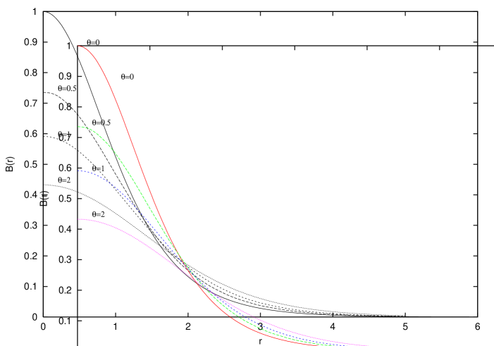
Figure 1: Magnetic field of a self-dual vortex as a function of the radial coordinate (in units of $\eta$) for different values of the anticommuting parameter $\theta$ (in units of $\eta^{2}$). The curve for $\theta=0$ coincides with that of the Nielsen-Olesen vortex in ordinary space.

We show in Figure 1 the resulting magnetic field $B$ as a function of $r\eta$. As explained above, one recovers for $\theta=0$ the result for self dual Nielsen-Olesen vortices in ordinary space[25]. As $\theta$ grows, the maximum for B decreases and the vortex is less localized with total area such that the magnetic flux remains equal to 1. It is important to stress that one finds noncommutative self-dual vortex solutions in the whole range of $\theta$, in agreement with the analysis for large and small $\theta$ presented in [27].

In ordinary space, anti-selfdual (negative flux) solutions can be trivially obtained from selfdual ones, just by making $B\to-B$, $\phi\to\bar{\phi}$. Now, the presence of the noncommutative parameter $\theta$, breaks parity and the moduli space for positive and negative magnetic flux vortices differ drastically. One has then to carefully study this issue in all regimes, not only for $\lambda=\lambda_{BPS}$ but also for $\lambda\neq\lambda_{BPS}$, when Bogomol’nyi equations do not hold and the second order equations of motion should be analyzed. Of course the recurrence relations associated to the second-order equations of motion become more complicated than (123)-(124); for example, for positive flux, they read

$$2(t_{n}f_{n+1}\;\sqrt{n+1+M}+t_{n-1}f_{n-1}\;\sqrt{n+M})+$$

$$(t^{2}_{n}+t^{2}_{n-1}+2n+2M+1)f_{n}=-\frac{{\theta{\eta}^{2}}{\lambda}}{2}f_{n}({f_{n}}^{2}-1)\;,\;\;n>1$$

$$(t_{n+1}^{2}-2t^{2}_{n}+t_{n-1}^{2})t_{n}={\theta}{\eta}^{2}\left(2f_{n}f_{n+1}\;{\sqrt{n+1+M}}+({f_{n}}^{2}+{f_{n+1}}^{2})t_{n}\right)\;,\;\;n>1$$

$$f_{1}=-\frac{f_{0}}{2t_{0}\sqrt{1+M}}\left((1+2M)+t_{0}^{2}+\frac{\theta\eta^{2}\lambda}{2}({f_{0}}^{2}-1)\right)$$

$$t_{1}^{2}=2t_{0}^{2}+\theta\eta^{2}\left((f_{1}^{2}+f_{0}^{2})t_{0}+2\sqrt{1+M}f_{0}f_{1}/t_{0}\right)$$ (138)

where we have slightly changed the definition of the gauge field coefficients just for notational convenience,

$$\hat{\phi} = \eta\sum_{n}f_{n}|n\rangle\langle n+M|$$

$${\hat{A}}_{z} = \frac{i}{\sqrt{\theta}}\sum_{n}(t_{n}+\sqrt{n+1})|n+1\rangle\langle n|$$ (139)

One can still solve this equations as for the simpler BPS case. We give below a summary of the main results[13, 14, 17]. As before, we take $\theta>0$ and distinguish positive from negative magnetic flux (this being equivalent to a classification of selfdual and anti-selfdual solutions).

• Positive flux

  1. There are BPS and non-BPS solutions in the whole range of $\eta^{2}\theta$. Their energy and magnetic flux are:

     For BPS solutions

     $$E_{BPS} = 2\pi\eta^{2}N\;,\;\;\;\Phi=2\pi N$$

     $$N = 1,2,\ldots$$ (140)

     For non-BPS solutions,

     $$E_{non-BPS} > 2\pi\eta^{2}N\;,\;\;\;\Phi=2\pi N$$

     $$N = 1,2,\ldots$$ (141)

  2. For $\eta^{2}\theta\to 0$ solutions become, smoothly, the known regular solutions of the commutative case.

  3. In the non-BPS case, the energy of an $N=2$ vortex compared to that of two $N=1$ vortices is a function of $\theta$.

  As in the commutative case, if one compares the energy of an $N=2$ vortex to that of two $N=1$ vortices as a function of $\lambda$ one finds that for $\lambda>\lambda_{BPS}$ $N>1$ vortices are unstable -they repel- while for $\lambda<\lambda_{BPS}$ they attract.

• Negative flux

  1. BPS solutions only exist in a finite range:

     $$0\leq\eta^{2}\theta\leq 1$$

     Their energy and magnetic flux are:

     $$E_{BPS} = 2\pi\eta^{2}N\;,\;\;\;\Phi=2\pi N$$

     $$N = 1,2,\ldots$$ (142)

  2. When $\eta^{2}\theta=1$ the BPS solution becomes a fluxon, a configuration which is regular only in the noncommutative case. The magnetic field of a typical fluxon solution takes the form

     $$B\sim\frac{1}{\sqrt{\theta}}{\exp(r^{2}/\theta)}$$ (143)

     We stressed above that for $\theta\to 0$ such a configuration becomes singular but note that in the present case the noncommutative parameter is fixed, $\theta=1/\eta^{2}\neq 0$.

  3. There exist non-BPS solutions in the whole range of $\theta$ but

     1. Only for $\theta<1$ they are smooth deformations of the commutative ones.

     2. For $\theta\to 1$ they tend to the fluxon BPS solution.

     3. For $\theta>1$ they coincide with the non-BPS fluxon solution.

Noncommutative instantons

The well-honored instanton equation

$$F_{\mu\nu}=\pm\tilde{F}_{\mu\nu}$$ (144)

was studied in the noncommutative case by Nekrasov and Schwarz[9] who showed that even in the $U_{*}(1)$ case one can find nontrivial instantons. The approach followed in that work was the extension of the ADHM construction, successfully applied to the systematic construction of instantons in ordinary space, to the noncommutative case. This and other approaches were discussed in [39]-[46]. Here we shall describe the methods developed in [15]-[16].

We work in four dimensional space where one can always choose

$$\theta_{12}=-\theta_{21}=\theta_{1}$$

$$\theta_{34}=-\theta_{43}=\theta_{2}$$

$${\rm all~{}other~{}}\theta^{\prime}s=0$$

We define dual tensors as

$$\tilde{F}_{\mu\nu}=\frac{1}{2}\sqrt{g}\,\varepsilon_{\mu\nu\alpha\beta}F^{\alpha\beta}$$ (145)

with $g$ the determinant of the metric.

In order to work in Fock space as we did in the case of noncommutative vortices, we now need two pairs of creation annihilation operators,

$$x^{1}\pm ix^{2}~{}~{}~{} {\Rightarrow} ~{}~{}~{}{\hat{a}}_{1},\;\;{\hat{a}}^{\;\dagger}_{1}$$

$$x^{3}\pm ix^{4}~{}~{}~{} {\Rightarrow} ~{}~{}~{}{\hat{a}}_{2},\;\;{\hat{a}}^{\;\dagger}_{2}$$

and the Fock vacuum will be denoted as $|00\rangle$. Concerning projectors the connection with configuration space takes the form

$$|n_{1}n_{2}\rangle\langle n_{1}n_{2}| {\Rightarrow} \exp\left(-r_{1}^{2}/\theta_{1}-r_{2}^{2}/\theta_{2}\right)L_{n_{1}}\left(2r_{1}^{2}/\theta_{1}\right)\times$$ (146)

$$L_{n_{2}}\left(2r_{2}^{2}/\theta_{2}\right)$$

Finally, note that the gauge group $SU(2)$ (for which ordinary instantons were originally constructed) should be replaced by $U(2)$ so that

$$A_{\mu}=A_{\mu}^{a}\frac{\sigma^{a}}{2}+A_{\mu}^{4}\frac{I}{2}$$ (147)

Let us now analyze how the different ansatz leading to ordinary instantons can be adapted to the noncommutative case.

i- (Commutative)’t Hooft multi-instanton ansatz (1976)

Gauge fields take value in the Lie algebra of $SU(2)$. They are written as

$$A_{\mu}(x)=\tilde{\Sigma}_{\mu\nu}j_{\nu}$$

$$\tilde{\Sigma}_{\mu\nu}=\frac{1}{2}\bar{\eta}_{a\mu\nu}\sigma^{a}\;,\;\;\;\bar{\eta}_{a\mu\nu}=\left\{\begin{array}[]{l}~{}\varepsilon_{a\mu\nu}\;,\;\;\;\mu,\nu\neq 4\\ ~{}~{}\delta_{a\mu}\;,\;\;\;\nu=4\\ -\delta_{a\nu}\;,\;\;\;\mu=4\end{array}\right.$$ (151)

$$j_{\nu}=\phi^{-1}\partial_{\nu}\phi$$

Here $\sigma^{a}$ are the Pauli matrices. With this ansatz, one can prove that

$$F_{\mu\nu}=\tilde{F}_{\mu\nu}+\frac{1}{\phi}\nabla\phi$$ (152)

so that if one can find a solution of the equation

$$\frac{1}{\phi}\nabla\phi=0$$ (153)

it will lead to a selfdual instanton configuration. The proposal of ’t Hooft was to take $\phi$ as

$$\phi=1+\sum_{i=1}^{N}\frac{\lambda_{i}^{2}}{(x-c_{i})^{2}}$$ (154)

with $c_{i}=(c_{i}^{\mu})$ and $\lambda_{i}$ real constants. Such a $\phi$ satisfies

$$\nabla\phi=\sum_{i=1}^{N}\delta^{(4)}(x-c_{i})$$ (155)

Now, each $\delta$-function singularity in $\nabla\phi$ is cancelled in (153) by the corresponding one in $\phi$ so that the equation is satisfied everywhere and selfduality in (152) is achieved. The solution corresponds to a regular instanton of topological charge $Q=N$. Points $c_{i}$ can be interpreted as the centers of spheres of radius $\lambda_{i}$ where one unit of topological charge is concentrated. One should note that the gauge field has singularities at points $x^{\mu}=c_{i}^{\mu}$ but these singularities are gauge removable and so the field strength is everywhere regular. For example, in the $Q=1$ case, the gauge field associated to ’t Hooft ansatz reads

$$A_{\mu}=-2\lambda^{2}\bar{\Sigma}_{\alpha\beta}\frac{x_{\beta}}{x^{2}(x^{2}+\lambda^{2})}$$ (156)

Since we have chosen $c_{1}=0$, the singularity is located at the origin. A (singular) gauge transformation leads to the regular version of (156),

$$A_{\mu}=-2\Sigma_{\alpha\beta}\frac{x_{\beta}}{(x^{2}+\lambda^{2})}$$ (157)

ii- Noncommutative version of ’t Hooft ansatz

To find a ’t Hooft-like ansatz for noncommutative instantons, one not only has to extend the proposal in the $SU(2)$ sector to the noncommutative case but one has also to include an ansatz for the $A_{\mu}^{4}$ component. A judicious choice is

$${A_{\mu}^{a}\frac{\sigma^{a}}{2}=\bar{\Sigma}_{\mu\nu}j_{\nu}}~{}~{}~{}\Rightarrow~{}~{}~{}A_{\mu}^{a}\frac{\sigma^{a}}{2}=\bar{\Sigma}_{\mu\nu}j_{\nu}\,,\;\;\;a=1,2,3$$ (159)

$$j_{\nu}=\phi^{-1}\partial_{\nu}\phi~{}~{}~{}\Rightarrow~{}~{}~{}j_{\nu}=\Phi^{-1}*\partial_{\nu}\Phi+\partial_{\nu}\Phi*\Phi^{-1}$$

(160)

$$A_{\mu}^{4}=-i\left(\Phi^{-1}*\partial_{\nu}\Phi-\partial_{\nu}\Phi*\Phi^{-1}\right)$$

The extension in (159)-(159) is the most natural one: ansatz (159) is just the one proposed by ’t Hooft and (159) is the symmetrized version, with respect to the $*$-product, of ’t Hooft current for ordinary products (Note that in the commutative limit $\Phi^{2}=\phi$). Concerning the completely new expression (160), it is the simplest ansatz, compatible with (159). In the commutative limit it corresponds to $A_{\mu}^{4}=0$ and, more important, it leads to a selfdual $F_{\mu\nu}^{4}$. This is not a trivial fact since $F_{\mu\nu}^{4}$ picks contributions not only from $A_{\mu}^{4}$ but also from $A_{\mu}^{a}\,,\;a=1,2,3$) but, strikingly, (160) ensures selfduality of $F_{\mu\nu}^{4}$ for any $\Phi$.

Now, one also needs selfduality of $F_{\mu\nu}^{a}$ with $a=1,2,3$. As in the case of $F_{\mu\nu}^{4}$, also the $SU(2)$ field strength picks contribution from $A_{\mu}^{4}$. After some work one can prove that

$$\tilde{F}_{\mu\nu}^{a}=F_{\mu\nu}^{a}+\eta_{\mu\nu a}\Phi^{-1}*\nabla\Phi^{2}*\Phi^{-1}$$ (161)

In the ordinary case, finding a solution of $\nabla\phi$ (which translates into $\nabla\Phi^{2}$ in the present case) was enough to ensure selfduality everywhere. Inspired in this fact, and noting that, as we learnt when studying fluxons one has, on the one hand

$$\lim_{\theta\to 0}\frac{1}{\theta}\exp\left(-\frac{r^{2}}{\theta}\right)\sim\delta(\vec{r})$$ (162)

and, on the other,

$$|00><00|\sim\frac{1}{\theta_{1}\theta_{2}}\exp\left(-\frac{r_{1}^{2}}{\theta_{1}}-\frac{r_{2}^{2}}{\theta_{2}}\right)$$ (163)

we can try to pose the problem in the form

$$\frac{1}{\phi}\nabla\phi=0~{}~{}~{}\Rightarrow~{}~{}~{}\Phi^{-1}*\nabla\Phi^{2}*\Phi^{-1}=0$$

$$\nabla\phi=\delta^{(4)}(x)\Rightarrow~{}~{}~{}\nabla\Phi^{2}=\frac{\lambda^{2}}{\theta_{1}\theta_{2}}|00\rangle\langle 00|$$ (164)

One easily finds the solution to the equation in the r.h.s. of (164). It reads (for simplicity we consider here the $N=1$ case and put $\theta_{1}=\theta_{2}=\theta$)

$$\Phi^{2}=1+\frac{\lambda^{2}}{r_{1}^{2}+r_{2}^{2}}\left(1-\exp\left(-\frac{r_{1}^{2}+r_{2}^{2}}{\theta}\right)\right)$$ (165)

where, say, $\vec{r}^{1}=(x^{0},x^{1})$ and $\vec{r}^{2}=(x^{2},x^{3})$. The Fock space version of (165) is

$$\Phi^{2}=1+\frac{\lambda^{2}}{2\theta}\sum\frac{1}{n_{1}+n_{2}+1}|n_{1}n_{2}\rangle\langle n_{1}n_{2}|$$ (166)

Now, in contrast with what happened in ordinary space, where $\phi^{-1}\nabla\phi=0$ one gets now

$$\Phi^{-1}\nabla\Phi^{2}\Phi^{-1}=-\frac{2\lambda^{2}}{\theta(2\theta+\lambda^{2})}|00\rangle\langle 00|$$ (167)

so that the field strength and its dual satisfies a relation of the form

$$F_{\mu\nu}=\tilde{F}_{\mu\nu}+\frac{2\lambda^{2}}{\theta(2\theta+\lambda^{2})}\tilde{\Sigma}|00\rangle\langle 00|$$ (168)

We see that the self-dual equation is not exactly satisfied: the $|00\rangle\langle 00|$ term, the analogous to the delta function in the ordinary case, is not cancelled as it happened with the delta function source for the Poisson equation (153) in the commutative case.

iii- Noncommutative BPST ($Q=1$) ansatz (1975)

The pioneering Belavin, Polyakov, Schwarz and Tyupkin ansatz[47] leading to the first $Q=1$ instanton solution was similar to the ’t Hooft ansatz except that $\Sigma_{\mu\nu}$ was used instead of its dual $\tilde{\Sigma}_{\mu\nu}$. Its noncommutative extension can be envisaged by writing, in the $SU(2)$ sector,

$${A_{\mu}^{a}\frac{\sigma^{a}}{2}=\Sigma_{\mu\nu}j_{\nu}}~{}~{}~{}\Rightarrow~{}~{}~{}A_{\mu}^{a}\frac{\sigma^{a}}{2}=\Sigma_{\mu\nu}j_{\nu}$$ (169)

where $j_{\nu}$ is defined as in the previous ansatz. Concerning $A_{\mu}^{4}$, the consistent ansatz changes due to the use of $\Sigma_{\mu\nu}$ instead of its dual as done in the ’t Hooft ansatz. One needs now, instead of (160),

$$A_{\mu}^{4}=i\left(\Phi^{-1}*\partial_{\nu}\Phi+3\partial_{\nu}\Phi*\Phi^{-1}\right)$$ (170)

With this, one finally has

$$F_{\mu\nu}=\tilde{F}_{\mu\nu}\;,\;\;\;Q=S=1$$ (171)

but, because of the necessity of a consistent ansatz for the $A_{\mu}^{4}$ component forces a factor “3” in the second term in the r.h.s. of eq.(170), one can see that

$$F_{\mu\nu}\neq F_{\mu\nu}^{\dagger}$$ (172)

and hence the price one is paying in order to have a selfdual field strength is its non-hermiticity. Note however that the action and the topological charge are real.

iv- (Commutative) Witten ansatz[48] (1977)

The clue in this ansatz is to reduce the four dimensional problem to a two dimensional one through an axially symmetric N-instanton ansatz. That is, one passes from $d=4$ Euclidan space to $d=2$ space with non trivial metric, $(x^{1},x^{2},x^{3},x^{4})\to(r,t)$.

The axially symmetric ansatz for the gauge field components is

$$\vec{A}_{r} = A_{r}(r,t)\vec{\Omega}(\vartheta,\varphi)$$

$$\vec{A}_{t} = A_{t}(r,t)\vec{\Omega}(\vartheta,\varphi)$$

$$\vec{A}_{\vartheta} = \phi_{1}(r,t)\partial_{\vartheta}\vec{\Omega}(\vartheta,\varphi)+\left(1+\phi_{2}(r,t)\right)\vec{\Omega}(\vartheta,\varphi)\wedge\partial_{\vartheta}\vec{\Omega}(\vartheta,\varphi)$$

$$\vec{A}_{\varphi} = \phi_{1}(r,t)\partial_{\varphi}\vec{\Omega}(\vartheta,\varphi)+\left(1+\phi_{2}(r,t)\right)\vec{\Omega}(\vartheta,\varphi)\wedge\partial_{\varphi}\vec{\Omega}(\vartheta,\varphi)$$ (173)

with

$$\vec{\Omega}(\vartheta,\varphi)=\left(\begin{array}[]{c}\sin\vartheta\cos\varphi\\ \sin\vartheta\sin\varphi\\ \cos\vartheta\end{array}\right)$$ (174)

With this ansatz the Yang-Mills action reduces to an Abelian-Higgs action in a curved space with metric

$$g^{ij}=r^{2}\delta^{ij}$$ (175)

$$\frac{1}{4}{\rm Tr}\int d^{4}xF_{\mu\nu}F_{\mu\nu} = \int_{-\infty}^{\infty}dt\int_{0}^{\infty}dr\sqrt{g}\left(\frac{1}{2}g^{ij}D_{i}\phi^{a}D_{j}\phi^{a}+\frac{1}{8}g^{ip}g^{jq}F_{ij}F_{pq}+\right.$$ (176)

$$\left.\frac{1}{4}(1-\left(\phi^{1})^{2}+(\phi^{2})^{2}\right)\right)$$

The selfduality instanton equations (144) associated to the Yang-Mills action become a pair of BPS equations for the gauge field -Higgs action in curved space,

$$F_{\mu\nu}=\tilde{F}_{\mu\nu} \to \left\{\begin{array}[]{l}\frac{1}{\sqrt{g}}F_{z\bar{z}}=|\phi|^{2}-1\\ D_{z}\phi=0\end{array}\right.$$ (179)

where $\phi=\phi_{1}+i\phi_{2}$ and $z=t+ir$. Moreover, solving these BPS vortex equations can be seen to reduce to finding the solution of a Liouville equation. In this way an exact axially symmetry N-instanton solution was constructed[48] for the (commutative) $SU(2)$ theory.

v- Noncommutative version of Witten ansatz

As we learnt in lecture 1, given a commutation relation of the form

$$[x^{i},x^{j}]=\theta^{ij}(x)$$ (180)

not all functions $\theta_{ij}(x)$ will guarantee a noncommutative but associative product. In the present 2 dimensional case we showed that a sufficient condiction for this was given by eq.(102),

$$\theta_{ij}=\theta_{0}\frac{\varepsilon_{ij}}{\sqrt{g}}$$ (181)

with $\theta_{0}$ a constant. Then, given the metric in which the instanton problem with axial symmetry reduces to a vortex problem we see that an associative noncommutative product should take the form

$$[r,t]=ir^{2}\theta_{0}$$ (182)

with now $r$ and $t$ defining the two dimensional variables in curved space. We then take this as the non-trivial commutation relation in the four-dimentional space from which the two-dimensional problem is inherited and put all the other commutation relations to zero,

$$[r,\vartheta]=[r,\varphi]=[\vartheta,\varphi]=[t,\vartheta]=[t,\varphi]=0$$ (183)

A further simplification occurs after the observation that

$$r*t-t*r=r^{2}\theta_{0}~{}~{}~{}\Rightarrow~{}~{}~{}t*\frac{1}{r}-\frac{1}{r}*t=\theta_{0}$$ (184)

Then, calling $y^{1}=t$ and $y^{2}=1/r$ we have instead of (182) the usual flat space Moyal product and the Bogomol’nyi equations take the form

$$\left(1-\frac{1}{2}(z+\bar{z})^{2}\right)D_{z}\phi = \left(1+\frac{1}{2}(z+\bar{z})^{2}\right)D_{\bar{z}}\phi$$ (185)

$$iF_{z\bar{z}} = 1-\frac{1}{2}[\phi,\bar{\phi}]_{+}$$ (186)

$$iF_{z\bar{z}} = -\frac{1}{2}[\phi,\bar{\phi}]$$ (187)

with $z=y^{1}+iy^{2}$. We can at this point apply the Fock space method detailed above for constructing vortex solutions. In the present case, consistency of eqs.(185)-(187) imply

$$\bar{\phi}\phi=1$$ (188)

and hence the only kind of nontrivial ansatz should lead, in Fock space, to a scalar field of the form

$$\phi=\sum_{n=0}|n+q\rangle\langle n|$$ (189)

where $q$ is some fixed positive integer. With this, it is easy now to construct a class of solutions analogous to those discussed in the context of fluxons in flat space. Indeed, a configuration of the form

$$\phi = \sum_{n=0}|n+q\rangle\langle n|$$

$$A_{z} = -\frac{i}{\sqrt{\theta_{0}}}\sum_{n=0}^{q-1}\left(\sqrt{n+1}\right)|n+1\rangle\langle n|+\frac{i}{\sqrt{\theta_{0}}}\sum_{n=q}\left(\sqrt{n+1-q}-\sqrt{n+1}\right)|n+1\rangle\langle n|$$

satisfies eqs.(185)-(187) provided $\theta_{0}=2$. In particular, both the l.h.s. and r.h.s of eq.(185) vanish separately. The field strength associated to this solution reads, in Fock space,

$$iF_{z\bar{z}}=-\frac{1}{2}\left(|0\rangle\langle 0|+\ldots+|q-1\rangle\langle q-1|\right)\equiv B$$ (191)

or, in the original spherical coordinates

$$\vec{F}_{tu} = B(r)\vec{\Omega}$$

$$\vec{F}_{\vartheta\varphi} = B(r)\sin\vartheta\,\vec{\Omega}$$

$$F_{tu}^{4} = B(r)$$

$$F_{\vartheta\varphi}^{4} = B(r)\sin\vartheta$$ (192)

As before, starting from (191) for $B$ in Fock space, we can obtain the explicit form of $B(r)$ in configuration space in terms of Laguerre polynomials, using eq.(146). Concerning the topological charge, it is then given by

$$Q = \frac{1}{32\pi^{2}}{\rm tr}\int d^{4}x{\varepsilon}^{\mu\nu\alpha\beta}F_{\mu\nu}F_{\alpha\beta}=\frac{1}{\pi}\int_{-\infty}^{0}du\int_{-\infty}^{\infty}dtB^{2}=2{\rm Tr}B^{2}=\frac{q}{2}$$ (193)

We thus see that $Q$ can be in principle integer or semi-integer, and this for an ansatz which is formally the same as that proposed in [48] for ordinary space and which yielded in that case to an integer. The origin of this difference between the commutative and the noncommutative cases can be traced back to the fact that in the former case, boundary conditions were imposed on the half-plane and forced the solution to have an associated integer number. In fact, if one plots Witten’s vortex solution in ordinary space in the whole $(r,t)$ plane, the magnetic flux has two peaks and the corresponding vortex number is even. Then, in order to parallel this treatment in the noncommutative case one should impose the condition $q=2N$.

Monopoles

Noncommutative monopoles cannot be found as simply as vortices or instantons by working in the Fock space framework. This is because creation-annihilation operator appear by pairs and monopole configurations should depend on 3 (not on 2 or 4) variables. However, it is known since the work of Manton[49] (see also [51]) that monopoles can be obtained as a particular limit of instanton solutions. The basic idea is the following: the instanton equation in 4-dimensional Euclidean space,

$$F_{\mu\nu}=\tilde{F}_{\mu\nu}$$ (194)

can be brought into the BPS monopole equation in 3-dimensional space,

$$F_{ij}^{a}=\varepsilon_{ijk}(D_{k}\phi)^{a}$$ (195)

by identifying

$$A_{0}^{a}=\phi^{a}$$ (196)

and eliminating in some way the dependence on Euclidean time. The connection between (194) and (195) is evident. Indeed, for space-space indices, (194) reads

$$F_{ij}=\varepsilon_{ijk}F_{k0}$$ (197)

Now, if gauge fields were time in dependent and moreover, we identify $A_{0}$ with $\phi$ according to (196), one gets (195).

The idea of Manton[49] was to start from Witten $N$-instanton solution which, as we have seen, is a sort of superposition of $1$-instantons located in different points of the time axis. Then, taking the $N\to\infty$ limit wipes out the dependence on time and hence in this limit the instanton configuration becomes time independent. One then has the desired connection,

$$\lim_{N\to\infty}(A_{i}^{N-inst}(\vec{x},t),A_{0}^{N-inst}(\vec{x},t))\;\;\;\Longrightarrow\;\;\;(A_{i}^{mon}(\vec{x}),\phi^{mon}(x))$$ (198)

This $N\to\infty$ has to be taken with care. Remember that the N-instanton was constructed by solving a vortex (Liouville) equation whose solution has poles located at certain points that we call $a_{i}$. In fact, the fundamental function from which the solution is constructed is

$$g(z)=\prod_{i=1}^{N}\frac{a_{i}-z}{\bar{a}_{i}+z}$$ (199)

The appropriate $N\to\infty$ limit should be taken for all points $a_{i}$ coinciding and taking the form

$$a_{i}=\frac{2N}{\beta}$$ (200)

with $\beta$ some scale so that

$$g(z)=\lim_{N\to\infty}\left(\frac{1-\beta z/2N}{1+\beta z/2N}\right)=\exp(-\beta z)$$ (201)

Let us take the same route but starting from our noncommutative solution. Rememeber that the magnetic field of the $d=2$ vortex in curved space was (191)

$$B^{q}==-\frac{1}{2}\left(|0\rangle\langle 0|+\ldots+|q-1\rangle\langle q-1|\right)$$ (202)

In the infinite ($q\to\infty$) limit, one clearly has

$$\lim_{q\to\infty}B^{q}=\frac{1}{2}$$ (203)

which is realized by the infinite charge limit of $A_{z}$ or

$$\lim_{q\to\infty}A_{1}=-\frac{y_{2}}{2}\;,\;\;\;\lim_{q\to\infty}A_{2}=\frac{y_{1}}{2}$$ (204)

In order to convert the self-duality instanton into a BPS monopole one has to identify $A_{2}=\phi$ and $(A_{1},A_{\varphi}A_{\vartheta})$ with the spatial components of the monopole. But one needs time-independence ($y_{2}$ independence) of the resulting fields and $A_{1}$ depends on time. In the ordinary case, one can easily gauge away this time dependence. Here, the affair becomes more involved: one has that $\theta=2$ and then one is in the peculiar situation discussed at the end of lecture 1 where gauge orbits could consist in just one point. Indeed, given the gauge field

$$A_{i}=\frac{1}{2}\varepsilon_{ij}y_{j}$$ (205)

a general gauge transformation takes the form

$$A_{i}^{g}=A_{i}+\left(1-\frac{\theta}{2}\right)g^{-1}*\partial_{i}g=A_{i}~{}~{}{\rm for}~{}\theta=2$$ (206)

One can however proceed to make a singular gauge transformation leading to the obvious time independent field configuration

$$A_{2}=-y_{1}\;,\;\;\;A_{2}=0$$ (207)

The transformation is

$$g=\exp_{x}(ic\Lambda)$$ (208)

with

$$\Lambda=\frac{1}{2}(\vec{\sigma}\cdot\vec{\Omega}+I)\;,\;\;\;c=\frac{1}{4}\log\left(1+\frac{\theta}{2}\right)$$ (209)

Calling $B_{i}$ the gauge transformed fields, we have that in the new gauge the only non-trivial fields are

$${\vec{B}}_{\varphi} = \frac{1}{2}(1+\cos\vartheta)\vec{\Omega}-\vec{\Omega}\wedge\partial_{\varphi}\vec{\Omega}$$

$$B_{\varphi}^{4} = -\frac{1}{2}(1+\cos\vartheta)$$

$$\vec{\phi} = \frac{B}{r}\Omega$$

$$\phi^{4} = \frac{B}{r}$$ (210)

Such a gauge field corresponds to a Wu-Yang monopole[51] (the non-Abelian version of the Dirac monopole) coupled to a Higgs scalar. It satisfies the Bogomol’nyi equation,

$$\frac{1}{2}\varepsilon^{ijk}\left(\partial_{j}A_{k}-\partial_{k}A_{j}+[A_{j},A_{j}]\right)=D^{i}\phi$$ (211)

In particular, if we define the “electromagnetic” field strength as usual,

$${\cal F}_{jk}={\rm Tr}\frac{\phi}{|\phi|}\left(\partial_{j}A_{k}-\partial_{k}A_{j}+[A_{j},A_{j}]\right)$$ (212)

we get the magnetic field off a Dirac monopole with unit charge,

$${\cal B}^{r}=\frac{\varepsilon^{r\vartheta\varphi}}{\sqrt{g}}{\cal F}_{\vartheta\varphi}=-\frac{1}{r^{2}}$$ (213)

Of course, the energy associated to this solution,

$$E={\rm Tr}\int d^{3}x\left(D_{i}\Phi D_{i}\Phi+\frac{1}{2}F_{ij}F_{ij}\right)$$ (214)

is strictly infinite (as it coincides with the selfenergy of a Dirac monopole)

$$E=\pi\int dr\frac{1}{r^{2}}=\int d^{3}xB_{mon}^{2}$$ (215)

Now, if we introduce a regulator $\epsilon$ to cut off the short-distances divergence and recover the dimensional scale $R$ ($\theta=\theta_{0}R^{2}=2R^{2}$) we can write $E$ in the form

$$E=\frac{\pi}{g_{YM}^{2}R\epsilon}=\frac{\pi R}{g_{YM}^{2}R^{2}\epsilon}=\frac{2\pi}{g_{YM}^{2}\theta}\frac{R}{\epsilon}$$ (216)

(We have reintroduced the gauge coupling constant $g_{YM}$ which was taken equal to 1 along the paper). Defining a length $L=R/\epsilon$ we see that $E$ can be identified with the mass of a string of length $L$ whose tension is

$$T=\frac{2\pi}{g_{YM}^{2}\theta}$$ (217)

One can see (214) as emerging in the decoupling linearized limit of a $D3$-brane in the Type IIB string theory with the Higgs field describing its fluctuations in a transverse direction. Since the $B$-field leading to our noncommutative setting is transverse to the $D3$-brane surface, one can make an analysis similar to that presented by Callan-Maldacena[52] with the scalar field describing a perpendicular spike. In this last investigation, where the electric case is discussed, the string interpretation corresponds to an $F$-string attached to a $D3$-brane. Our magnetic case can be related to this by an $S$-duality transformation changing the $F1$ into a $D1$ string. Comparing the tension of such a $D1$-string with the one resulting from our solution (eq.(217)),

$$T_{D1}=\frac{1}{2\pi\alpha^{\prime}g_{s}}=\frac{2\pi}{g_{YM}^{2}\theta}$$ (218)

and using $2\pi g_{s}=g^{2}_{YM}$ we see that quantization of the magnetic monopole charge leads to a quantized value for $\theta$ in string length units equal to $1$ for our charge-1 monopole, $\theta/2\pi\alpha^{\prime}=1$.

4 Noncommutative Theories in d=2,3 dimensions

The Seiberg-Witten map

This is an explicit map connecting a given noncommutative gauge theory with a conventional gauge theory. Consider the case in which the noncommutative gauge theory is governed by a Yang-Mills (YM) Lagrangian for the gauge potential $\hat{A}_{\mu}$, transforming under gauge rotations according to

$$\hat{\delta}_{\hat{\varepsilon}}A_{\mu}(x)=\hat{A}^{\prime}_{\mu}(x)-\hat{A}_{\mu}(x)=D_{\mu}[\hat{A}]\hat{\varepsilon}(x)$$ (219)

The Seiberg-Witten map connects the noncommutative YM Lagrangian to some unconventional Lagrangian on the commutative side. What is conventional in the latter, apart from the fact taht fields are multiplied with the ordinary product is that the transformation law for the gauge field $A_{\mu}$ is governed by the ordinary covariant derivative,

$$\delta_{\varepsilon}A_{\mu}(x)=A^{\prime}_{\mu}(x)-A_{\mu}(x)=D_{\mu}[A]\varepsilon(x)$$ (220)

Note that we are calling $\hat{\varepsilon}$, the infinitesimal gauge transformation parameter in the noncommutative theory to distinguish it from $\varepsilon$, its mapped relative in the ordinary theory. Hence, the mapping should include, appart from a connection between $\hat{A}_{\mu}$ and $A_{\mu}$, one for connecting $\hat{\varepsilon}$ and $\varepsilon$.

The equivalence should hold at the level of orbit space, the physical configuration space of gauge theories. This means that if two gauge fields $\hat{A}_{\mu}$ and $\hat{A}^{\prime}_{\mu}$ belonging to the same orbit can be connected by a noncommutative gauge transformation $\exp_{*}(i\hat{\varepsilon})$, then $A^{\prime}_{\mu}$ and $A_{\mu}$, the corresponding mapped gauge fields will also be gauge equivalent by an ordinary gauge transformetion $\exp(i\varepsilon)$. An important point is that the mapping between $\hat{\varepsilon}$ and $\varepsilon$ necessarily depends on $A_{\mu}$. Indeed, were $\hat{\varepsilon}$ a function solely of $\varepsilon$, the ordinary and the noncommutative gauge groups would be identical. That this is not possible can be seen just by considering the case of a $U(1)$ gauge theory in which, through a redefinition of the gauge parameter, one would be establishing an isomorphism between non commutative $U_{*}(1)$ and commutative $U(1)$ gauge groups.

Then, the Seiberg-Witten mapping consists in finding

$$\hat{A} = \hat{A}[A;\theta]$$

$$\hat{\varepsilon} = \hat{\varepsilon}[\varepsilon,A;\theta]$$ (221)

so that the equivalence between orbits holds,

$$\hat{A}[A]+\hat{\delta}_{\hat{\varepsilon}}\hat{A}[A]=\hat{A}[A+\delta_{\varepsilon}A]$$ (222)

Using the explicit form of gauge transformations and expanding to first order in $\theta=\delta\theta$, the solution of (222) reads

$$\hat{A}_{\mu}[A]=A_{\mu}-\frac{1}{4}\delta\theta_{\rho\sigma}[A_{\rho},\partial_{\sigma}A_{\mu}+F_{\sigma\mu}]_{+}+O(\delta\theta^{2})$$

$$\hat{\varepsilon}[\varepsilon,A]=\varepsilon+\frac{1}{4}\delta\theta_{\rho\sigma}[\partial_{\rho},A_{\sigma}]_{+}+O(\delta\theta^{2})$$ (223)

Concerning the field strength, the connection is given by

$$\hat{F}_{\mu\nu}[A]=F_{\mu\nu}+\frac{1}{4}\delta\theta^{\alpha\beta}\left(2[F_{\mu\alpha},F_{\nu\beta}]_{+}-[A_{\alpha},D_{\beta}F_{\mu\nu}+\partial_{\beta}F_{\mu\nu}]_{+}\right)$$ (224)

One can interpret these equations as differential equations describing the passage from $A_{\mu}^{\theta}$, the gauge field in a theory with parameter $\theta$ to $A_{\mu}^{\theta+\delta\theta}$, the gauge field in a theory with parameter $\theta+\delta\theta$. Integrating of such equations one determines, to all orders in $\theta$, how one passes from $L_{YM}[\hat{A}]$ the noncommutative version of Yang-Mills Lagrangian, to $L[A,\theta]$ a complicated but commutative equivalent Lagrangian.

Fermion models in two dimensional space and the W*Z*W model

It is well-known that for two-dimensional field theories, one can establish a connection, called bosonization (fermionization), that allows to connect a given fermion (boson) model with certain bosonic (fermionic) counterpart. This means that any physical quantity that can be computed for the fermionic model can be alternatively computed for the bosonic model. Physical quantities are constructed from correlation functions of products of currents and product of energy-mementum tensor components (which in turn can be expressed in terms of currents). The so called bosonization/fermionization recipe is nothing but a dictionary that tells how to connect the Lagrangian and the currents in one language to the Lagrangian and the currents in the other. Also, there is a connection between coupling constants in the two models and, remarkably, the weak coupling regime in one language corresponds to strong-coupling regime in the other. This last property attracted, during the 1970’s and 1980’s, a lot of people working in field theory and particle physics since bosonization provided a simplified laboratory where untractable non-perturbative calculations could be more easily handled perturbatively just by working in the equivbalen theory.

Non-Abelian bosonization (i.e., bosonization of a fermion model with non-Abelian symmetry) was achieved in 1983 by Witten[53] who showed that a a two-dimensional theory of fermions $\psi$ in some representation of a non-Abelian group $G$ translates into a bosonic theory where fields $a$ are group valued, $a\in G$. The connection of the corresponding actions takes the form

  bosonization/fermionization

Figure 2: The bosonization/fermionization recipe connects the free fermion action with a Wess-Zumino-Witten action

Here, the Wess-Zumino-Witten action is given by

$$WZW[a]=\frac{1}{4\pi}{\rm tr^{c}}\!\!\int\!\!d^{2}x\left(\partial_{\mu}a^{-1}\right)\left(\partial_{\mu}a\right)+\frac{i}{6\pi}\varepsilon_{ijk}{\rm tr^{c}}\!\!\int_{B}\!\!d^{3}ya^{-1}(\partial_{i}a)a^{-1}(\partial_{j}a)a^{-1}(\partial_{k}a)$$

where $B$ is a 3-dimensional manifold which in compactified Euclidean space can be identified with a ball with boundary $S^{2}$. Index $i$ runs from 1 to 3.

The question we would like to pose is whether there exist a noncommutative version of the bosonization recipe. That is, a connection of the form

  bosonization/fermionization

Figure 3: A bosonization/fermionization recipe for noncommutative two dimensional models

where the noncommutative version of Wess-Zumino-Witten action would be

$$WZW[\hat{a}] = \frac{1}{4\pi}{\rm tr^{c}}\!\!\int\!\!d^{2}x\left(\partial_{\mu}\hat{a}^{-1}\right)*\left(\partial_{\mu}\hat{a}\right)+$$ (226)

$$\frac{i}{6\pi}\varepsilon_{ijk}{\rm tr^{c}}\!\!\int_{B}\!\!d^{3}y\hat{a}^{-1}*(\partial_{i}\hat{a})*\hat{a}^{-1}*(\partial_{j}\hat{a})*\hat{a}^{-1}*(\partial_{k}\hat{a})$$

where fields $\hat{a}$ are group valued, $\hat{a}\in G_{*}$. Now, the noncommutative fermion action in the left hand side of figure 3 being quadratic, it should be equivalent to the ordinary fermion action while the bosonic Wess-Zumino-Witten action in the r.h.s. contains cubic terms which cannot be trivially reduced to the commutative cubic terms of an ordinary WZW action. However, going counter clockwise as indicated in figure 4, one could in principle pass from noncommutative to ordinary WZW actions,

Figure 4: Connections between commutative and noncommutative two dimensional models

We shall clarify this issue using the path integral approach to bosonization. This requires as a first step the knowledge of the two dimensional (noncommutative) fermion determinant in a background vector field. For simplicity, we shall consider in detail the $U_{*}(1)$ model and then extend the treatment to the full $U_{*}(N)$ case.

The fermion determinant: the $U_{*}(1)$ case

We now proceed to the exact calculation of the effective action for noncommutative $U_{*}(1)$ fermions in the fundamental representation as first presented in refs.[11]-[12], by integrating the chiral anomaly. Indeed, taking profit that in 2 dimensions a gauge field $A_{\mu}$ can always be written in the form[54]

$$\not\!\!A=-\frac{1}{e}\left(i\!\!\not\!\partial U[\phi,\eta]\right)*U^{-1}[\phi,\eta]$$ (227)

with

$$U[\phi,\eta]=\exp_{*}(\gamma_{5}\phi+i\eta)\,,$$ (228)

one can relate the fermion determinant in a gauge field background $A_{\mu}$ with that corresponding to $A_{\mu}=0$ making a decoupling change of variables in the fermion fields. For simpolicity, we consider here the case of fermions in the fundamental representation (but calculations go the same in the other two cases). The appropriate change of fermionic variables is

$$\psi\to U[\phi,\eta]*\psi\,,\hskip 56.9055pt\bar{\psi}\to\bar{\psi}*U^{-1}[\phi,\eta]$$ (229)

One gets[55]

$${\det}(\not\!\partial-ie\!\!\not\!\!A)=\det\not\!\partial\exp\left(-2\int_{0}^{1}dt\frac{dJ^{f}[t\phi,A]}{dt}\right)$$ (230)

where $J^{f}[t\phi,A]$ is the Fujikawa Jacobian associated with a transformation $U_{t}$ where $t$ is a parameter, $0\leq t\leq 1$, such that

$$U_{0} = 1$$

$$U_{1} = U[\phi,\eta]$$ (231)

Computation of the Jacobian $J^{f}[t\phi,A]$ for such finite transformations $U_{t}$ can be done after evaluation of the chiral anomaly, related to infinitesimal transformations. Indeed, consider an infinitesimal local chiral transformation which in the fundamental representation reads

$$\delta_{\epsilon}^{5}\psi = i\gamma_{5}\epsilon(x)*\psi(x)$$ (232)

The chiral anomaly ${\cal A}={\cal A}^{a}t^{a}$, associated with the non-conservatyion of the chiral current $j^{a\mu}_{5}$

$$j^{a\mu}_{5}=\bar{\psi}\gamma_{5}t^{a}\psi$$ (233)

$$\partial_{\mu}j^{a\mu}_{5}={\cal A}^{a}[A]\,,$$ (234)

can be calculated from the Fujikawa Jacobian $J[\epsilon,A_{\mu}]$ associated with infinitesimal transformation (232),

$$\log J[\epsilon,A_{\mu}]=-2{\rm tr^{c}}\!\!\int\!\!d^{2}x{\cal A}[A]\epsilon(x)=\left.-2{\rm tr^{c}}\!\!\int\!\!d^{2}x{\rm Tr}\left(\gamma_{5}\epsilon(x)\right)\right|_{reg}$$ (235)

Here Tr means both a trace for Dirac matrices and a functional trace in the space on which the Dirac operator acts. With ${\rm tr}^{c}$ we indicate a trace over the gauge group indices and with reg we stress that some regularization prescription should be adopted to render finite the Tr trace. We shall adopt the heat-kernel regularization, this meaning that

$${\cal A}[A]=\lim_{M^{2}\to\infty}{\rm Tr}\left(\gamma_{5}\exp_{*}\left(\frac{\gamma^{\mu}\gamma^{\nu}D_{\mu}*D_{\nu}}{M^{2}}\right)\right)$$ (236)

The covariant derivative in the regulator has to be chosen among those defined by eqs.(76)-(78) according to the representation one has chosen for the fermions. Concerning the fundamental representation, the anomaly has been computed following the standard Fujikawa procedure[12].

$${\cal A}^{f}[A]=\frac{e}{4\pi}\varepsilon^{\mu\nu}F_{\mu\nu}$$ (237)

(We indicate with $f$ that the fundamental representation has been considered). Analogously, one obtains for the anti-fundamental representation

$${\cal A}^{\bar{f}}[A]=-\frac{e}{4\pi}\varepsilon^{\mu\nu}F_{\mu\nu}$$ (238)

Now, writing $\epsilon=\phi dt$, we can use the results given through eqs.(235)-(237) to get, for the Jacobian,

$$\log J^{f}[t\phi,A]=-\frac{e}{2\pi}{\rm tr^{c}}\int d^{2}x\varepsilon_{\mu\nu}F^{t}_{\mu\nu}*\phi$$ (239)

where

$$F^{t}_{\mu\nu}=\partial_{\mu}A_{\nu}-\partial_{\nu}A_{\mu}-ie\{A^{t}_{\mu},A_{\nu}^{t}\}$$ (240)

$$\gamma^{\mu}A_{\mu}^{t}=-\frac{1}{e}\left(i\!\!\not\!\partial U_{t}\right)*U_{t}^{-1}$$ (241)

This result can be put in a more suggestive way in the light cone gauge where

$$A_{+} = 0$$

$$A_{-} = g(x)*\partial_{-}g^{-1}(x)$$

$$g(x) = \exp_{*}(2\phi)$$ (242)

Indeed, in this gauge one can see that (230) becomes

$$\log \left(\frac{{\det}(\not\!\partial-ie\!\!\not\!A)}{{\det}\not\!\partial}\right)=\log J^{f}[t\phi,A]=-\frac{1}{8\pi}{\rm tr^{c}}\int d^{2}x\left(\partial_{\mu}g^{-1}\right)*\left(\partial_{\mu}g\right)$$ (243)

$$+\frac{i}{12\pi}\varepsilon_{ijk}{\rm tr^{c}}\int_{B}d^{3}yg^{-1}*(\partial_{i}g)*g^{-1}*(\partial_{j}g)*g^{-1}*(\partial_{k}g)$$

Here we have written $d^{3}y=d^{2}xdt$ so that the integral in the second line runs over a 3-dimensional manifold $B$ which in compactified Euclidean space can be identified with a ball with boundary $S^{2}$. Index $i$ runs from 1 to 3. The $*$ product on $B$ is the trivial extension of the noncommutative product defined in the original two dimensional manifold, with the extra dimension taken to be commutative. Concerning the anti-fundamental representation, the calculation of the fermion determinant follows identical steps. Using the expression of the anomaly given by (238), one computes the determinant which coincides with that in the fundamental representation (remember that the anomaly is proportional to the charge $e$ while the determinant to $e^{2}$).

For the Dirac operator in the adjoint representation, one starts from the Dirac action which takes the form

$$S_{f}=\int d^{2}x\bar{\psi}*i\gamma^{\mu}\left(\partial_{\mu}\psi+ie\{A_{\mu},\psi\}\right)$$ (244)

Writing the field $A_{\mu}$ as in equation (227) (for simplicity we will work in the gauge $\eta=0$) and making again a change of the fermion variables to decouple the fermions from the gauge fields

$$\psi=e^{\gamma^{5}\{\phi,\cdot\}}*\chi=\chi+\gamma^{5}\{\phi,\chi\}+\frac{1}{2}\{\phi,\{\phi,\chi\}\}+\cdots$$

$${\bar{\psi}}={\bar{\chi}}*e^{\{\cdot,\phi\}\gamma^{5}}={\bar{\chi}}+\{{\bar{\chi}},\phi\}\gamma^{5}+\frac{1}{2}\{\{{\bar{\chi}},\phi\},\phi\}+\cdots$$ (245)

one has

$${\det}(\not\!\partial+ie\gamma\cdot[A,\cdot]_{*})=\det\not\!\partial\exp\left(-2\int_{0}^{!}dt\frac{dJ^{ad}[t\phi,A]}{dt}\right)$$ (246)

where $J^{ad}[t\phi,A]$ is the Fujikawa Jacobian associated with a transformation for fermions in the adjoint (245),

$$\psi=e^{\gamma^{5}[t\phi,\cdot]_{*}}*\chi$$

$${\bar{\psi}}={\bar{\chi}}*e^{[\cdot,t\phi]_{*}\gamma^{5}}$$ (247)

Following the same procedure as before, one finds that

$$\frac{d}{dt}\log(J^{ad})=\int d^{2}x\;{\cal A}(x)*\phi(x)$$ (248)

where

$${\cal A}(x)=2\lim_{M\to\infty}{\rm tr}\;\gamma^{5}\;\int_{k}\exp_{*}({-ik\cdot x})\exp_{*}\left({\not\!\!D^{2\;Ad}/M^{2}}\right)\exp_{*}({ik\cdot x})$$ (249)

After a straightforward computation, one can prove the following identity

$$\exp_{*}({-ik\cdot x})\exp_{*}\left(\not\!\!D_{Ad}^{2}/M^{2}\right)\;\exp_{*}({ik\cdot x})=\exp_{*}\left((\not\!\!D_{Ad}+i\not\!k+ie\not\!c)^{2}/M^{2}\right)$$ (250)

where

$$c_{\mu}(x;k) = -2i\int_{p}\;\exp_{*}\left({-ip\wedge k}\sin(p\wedge k)\right)A_{\mu}(p)\exp_{*}({ip\cdot x})$$ (251)

$$= A_{\mu}(x-\theta\cdot k)-A_{\mu}(k)$$

Finally, expanding the exponent up to order $M^{-2}$, taking the trace and integrating over $d^{2}k$ we have

$${\cal A}(x)=-\frac{e}{\pi}\lim_{M\to\infty}\;\int_{p}\;\left((1-\exp_{*}\left({-M^{2}\theta^{2}p^{2}/4}\right)\right)\epsilon_{\mu\nu}F_{\mu\nu}(p)\exp_{*}({ip\cdot x})$$ (252)

Notice that if we take the $\theta\to 0$ limit before taking the $M\to\infty$ limit ${\cal A}$ vanishes and the Jacobian is $1$, so we recover the standard (commutative) result which corresponds to a trivial determinant for the trivial $U(1)$ covariant derivative in the adjoint. Now, the limits $\theta\to 0$ and $M\to\infty$ do not commute so that if one takes the $M^{2}\to\infty$ limit at fixed $\theta$ one has the $\theta$-independent result

$$\frac{d}{dt}\log J^{Ad}[t\phi,A]=-\frac{e}{\pi}\int d^{2}x\varepsilon_{\mu\nu}F^{t}_{\mu\nu}*\phi$$ (253)

which is twice the result of the fundamental representation. The integral in $t$ is identical to the one of the fundamental representation so we finally have

$$\log \left(\frac{{\det}\left(\not\!\partial-ie\gamma_{\mu}\{A_{\mu},~{}\}\right)}{{\det}\not\!\partial}\right)=-\frac{1}{4\pi}{\rm tr^{c}}\int d^{2}x\left(\partial_{\mu}g^{-1}\right)*\left(\partial_{\mu}g\right)$$ (254)

$$+\frac{i}{6\pi}\varepsilon_{ijk}{\rm tr^{c}}\int_{B}d^{3}yg^{-1}*(\partial_{i}g)*g^{-1}*(\partial_{j}g)*g^{-1}*(\partial_{k}g)$$

Comparing this result with that in the fundamental, we see that we have proven the formula

$$\Gamma^{Adj}=2\;\Gamma^{Fund}$$ (255)

This is reminiscent of the relation that holds when one compares the anomaly and the fermion determinant for commutative two-dimensional fermions in a gauge field background, for the fundamental and the adjoint representation of $U(N)$. In this last case, there is a factor relating the results in the adjoint and the fundamental which corresponds to the quadratic Casimir $C(G)$ in the adjoint[56] (see for example [57] for a detailed derivation). Now, it was observed [58] that diagrams in noncommutative $U_{*}(1)$ gauge theories could be constructed in terms of those in ordinary non-Abelian gauge theory with $C(G)=2$; this is precisely what we have found in the present case.

We can stop at this point and recapitulate, using figure 4, the results we have obtained: as indicated in the upper part of the figure, we have connected the noncommutative fermion action with the noncommutative version of the Wess-Zumino-Witten action which we suggestively write as $W*Z*W$. The fact that the fermion action is quadratic allows us to descend to the ordinary level from the left of the figure and bosonization connect this with an ordinary $WZW$ action. The lacking link to close the loop in figure 4 should then be a Seiberg-Witten like map except that in the present case it will not be related to gauge symmetry but to the relevant symmetry in WZW theories. Moreover, it will not connect two completely different Lagrangians but the two versions (commutative and noncommutative) of the same Lagrangian.

The Seiberg-Witten map for W*Z*W models

Before study the mapping between the non-commutative and standard WZW theories, let us mention some properties of the Moyal deformation in two dimensions.

Equation (6) can be re-written in term of holomorphic and anti-holomorphic coordinates in the form:

$$\left.\phi(z,{\bar{z}})*\chi(z,{\bar{z}})=\exp\left\{\theta(\partial_{z}\partial_{\bar{w}}-\partial_{\bar{z}}\partial_{w})\right\}\phi(z,{\bar{z}})\chi(w,{\bar{w}})\right|_{w=z}$$ (256)

This formula simplifies considerably in two particular cases. First, when one of the functions is holomorphic (anti-holomorphic) and the other is anti-holomorphic (holomorphic), the deformed product reads as

$$\phi(z)*\chi(\bar{z})=e^{\theta\partial_{z}\partial_{\bar{z}}}\phi(z)\;\chi(\bar{z})\;,\hskip 28.45274pt\phi(\bar{z})*\chi(z)=e^{-\theta\partial_{z}\partial_{\bar{z}}}\phi(\bar{z})\;\chi(z)\;$$ (257)

and the deformation is produced by an overall operation over the standard (commutative) product with no $w\to z$ limit necessary.

Second, when both functions are holomorphic (anti-holomorphic), the star product coincides with the regular product

$$\phi(z)*\chi(z)=\phi(z)\chi(z)\;,\hskip 28.45274pt\phi({\bar{z}})*\chi({\bar{z}})=\phi({\bar{z}})\chi({\bar{z}})\;.$$ (258)

That means that the holomorphic or anti-holomorphic sectors of a two-dimensional field theory are unchanged by the deformation of the product. For example, the holomorphic fermionic current in the deformed theory takes the form,

$$\hat{j}_{z}=\psi^{\dagger}_{R}\;*\psi_{R}\;.$$ (259)

And since $\psi_{R}$ has no ${\bar{z}}$ dependence on-shell, the deformed current coincides with the standard one

$$j_{z}=\psi^{\dagger}_{R}\;\psi_{R}\;.$$ (260)

Moreover, since the free actions are identical, any correlation functions of currents in the standard and the $*$-deformed theory will be identical.

This last discussion tell us that, since the WZW actions are the generating actions of fermionic current correlation functions, both actions (standard and non-commutative) are equivalent. It remains to see if we can link both actions through a Seiberg-Witten like mapping. Let us try that.

Consider the noncommutative W*Z*W action, $W*Z*W[\hat{g}]$, with $\hat{g}$ the gauge group element when the deformation parameter is $\theta$. The action is invariant under chiral holomorphic and anti-holomorphic transformations

$$\hat{g}\rightarrow\bar{\Omega}({\bar{z}})\hat{g}\;\Omega(z)$$ (261)

so in analogy with the Seiberg-Witten mapping we will look for a transformation that maps respectively holomorphic and anti-holomorphic “orbits” into “orbits”. Of course the analogy breaks down at some point as this holomorphic and anti-holomorphic “orbits” are not equivalence classes of physical configurations, but just symmetries of the action. However we will see that such a requirement is equivalent, in some sense, to the “gauge orbits preserving transformation condition” of Seiberg-Witten.

Thus, we will find a transformation that maps a group-valued field $\hat{g}^{\prime}$ defined in non-commutative space with deformation parameter $\theta^{\prime}$ to a group-valued field $\hat{g}$, with deformation parameter $\theta$. We demand this transformation to satisfy the condition

$$\bar{\Omega}^{\prime}(\bar{z})*^{\prime}\hat{g}^{\prime}*^{\prime}\Omega^{\prime}(z)\to\bar{\Omega}(\bar{z})*\hat{g}*\Omega(z)$$ (262)

where the primed quantities are defined in a $\theta^{\prime}$-non-commutative space and the non primed quantities defined in a $\theta$-non-commutative space. In particular this mapping will preserve the equations of motion:

$$\hat{g}^{\prime}=\alpha^{\prime}*^{\prime}\beta^{\prime}\to\hat{g}=\alpha*\beta$$ (263)

The simplest way to achieve this, by examining equation (257) is defining

$$\hat{g}[\theta]=e^{-\theta\partial_{z}\partial_{\bar{z}}}\;g[0]$$ (264)

or, infinitesimally

$$\frac{d\hat{g}}{d\theta}=-\partial_{z}\partial_{\bar{z}}\;\hat{g}$$ (265)

However, the corresponding transformation for ${\hat{g}}^{-1}$ is more cumbersome

$$\frac{d{\hat{g}}^{-1}}{d\theta}=\partial_{z}\partial_{\bar{z}}\;{\hat{g}}^{-1}+2\partial_{\bar{z}}({\hat{g}}^{-1}*\partial_{z}\hat{g})*{\hat{g}}^{-1}$$ (266)

So let us consider a more symmetric transformation, that coincides on-shell, with (265) and (266). Consider thus

$$\frac{d\hat{g}}{d\theta} = \hat{g}*\partial_{\bar{z}}\;{\hat{g}}^{-1}*\partial_{z}\hat{g}$$

$$\frac{d{\hat{g}}^{-1}}{d\theta} = -\partial_{z}{\hat{g}}^{-1}*\partial_{\bar{z}}\hat{g}*{\hat{g}}^{-1}$$ (267)

These equations satisfy the condition (262) for functions $\Omega(z)$ and $\bar{\Omega}(\bar{z})$ independent of $\theta$. Indeed we have, for example

$$\frac{d(\hat{g}*\Omega(z))}{d\theta} = \frac{d\hat{g}}{d\theta}*\Omega(z)-\partial_{\bar{z}}\hat{g}*\partial_{z}\Omega(z)$$ (268)

$$= (\hat{g}*\Omega(z))*\partial_{\bar{z}}\;(\hat{g}*\Omega(z))^{-1}*\partial_{z}(\hat{g}*\Omega(z))$$

and a similar equation for the anti-holomorphic transformation.

The next step is to see how does the WZW action transforms under this mapping. First consider the variation of the following object:

$$\omega={\hat{g}}^{-1}*\delta\hat{g}$$ (269)

where $\delta$ is any variation that does not acts on $\theta$.

After a straightforward computation we find that

$$\frac{d\omega}{d\theta}=-\partial_{\bar{z}}\omega*j_{z}-j_{z}*\partial_{\bar{z}}\omega$$ (270)

where

$$j={\hat{g}}^{-1}*\partial_{z}\hat{g}$$ (271)

is the holomorphic current. In particular we have

$$\frac{dj_{z}}{d\theta}=-\partial_{\bar{z}}j_{z}*j_{z}-j_{z}*\partial_{\bar{z}}j_{z}=-\partial_{\bar{z}}(j_{z}^{2})$$ (272)

Similarly we can find the variations for

$$\bar{\omega}=\delta\hat{g}*{\hat{g}}^{-1}$$ (273)

and we get

$$\frac{d\bar{\omega}}{d\theta} = \partial_{z}\omega*j_{\bar{z}}+j_{\bar{z}}*\partial_{z}\bar{\omega}$$

$$\frac{dj_{\bar{z}}}{d\theta} = \partial_{z}j_{\bar{z}}*j_{\bar{z}}+j_{\bar{z}}*\partial_{z}j_{\bar{z}}=\partial_{z}(j_{\bar{z}}^{2})$$ (274)

where

$$j_{\bar{z}}=\partial_{\bar{z}}\hat{g}*{\hat{g}}^{-1}.$$ (275)

Note that on-shell, both $j_{z}$ and $j_{\bar{z}}$ are $\theta$-independent, that is the non-commutative currents coincide with the standard ones. This result is expected since the same happens for their fermionic counterparts.

Now, instead of studying how does the $\theta$-map acts on the WZW action, it is easy to see how does the mapping acts on the variation of the WZW action with respect to the fields. In fact, we have

$$\delta W[\hat{g}]=\frac{k}{\pi}\int d^{2}x\;{\rm tr}\left(\partial_{\bar{z}}j_{z}\;\omega\right)$$ (276)

where $j_{z}$ and $\omega$ are the quantities defined in eqs.(269) and (271) and there is no $*$-product between them in eq.(276) in virtue of the quadratic nature of the expression.

Thus, a simple computation shows that

$$\frac{d\;\delta W[\hat{g}]}{d\theta}=0$$ (277)

and we have a remarkable result: the transformation (267), integrated between $0$ and $\theta$ maps the standard commutative WZW action into the noncommutative WZW action. That is, we have found a transformation mapping orbits into orbits such that it keeps the form of the action unchanged provided one simply performs a $\theta$-deformation. This should be contrasted with the 4 dimensional noncommutative Yang-Mills case for which a mapping respecting gauge orbits can be found (the Seiberg-Witten mapping) but the resulting commutative action is not the standard Yang-Mills one. However, one can see that the mapping (267) is in fact a kind of Seiberg-Witten change of variables.

Indeed, if we consider the WZW action as the effective action of a theory of Dirac fermions coupled to gauge fields, as we did in previous sections, instead of an independent model, we can relate the group valued field $g$ to gauge potentials. As we showed in eq.(242), this relation acquires a very simple form in the light-cone gauge $A_{+}=0$ where

$$A_{-}=\hat{g}(x)*\partial_{-}{\hat{g}}^{-1}(x)\;.$$ (278)

But notice that in this gauge, $A_{-}$ coincides with $j_{\bar{z}}$ (eq.(275), so we have from equation (274)

$$\delta A_{-}=\delta\theta\left(\partial_{z}A_{-}*A_{-}+A_{-}*\partial_{z}A_{-}\right)$$ (279)

which is precisely the Seiberg-Witten mapping in the gauge $A_{+}=0$.

The loop in figure 4 is now closed

C*S theory in d=3 dimensions

The W*Z*W action was obtained by computing the fermion determinant of the Direc operator for $d=2$ noncommutative fermions coupled to a gauge-field background. Thus, it is natural to compute the same determinant, but in $d=3$ spacetime. This was done by Grandi and Silva[62] and we shall briefly describe the results they have found. For simplicity, we take massive fermions so that a $\partial/m$ expansion can be easily used to compute the parity odd part of the determinant.

Coupling fermions to a gauge field $A_{\mu}$ in the Lie Algebra of $U_{*}(N)$, the action reads

$$S(\bar{\psi},\psi,A;m)\;=\;\int d^{3}x\;{\bar{\psi}}({x})*(i\not\!\!D[A]-m)({x})\;.$$ (280)

and again we have three possibilities for the Dirac operator

$$\psi(x)\to\left\{\begin{array}[]{ll}g(x)*\psi(x)&${\rm fundamental representation} $``f"$ $\\ \psi(x)*g^{-1}(x)&${\rm anti-fundamental representation} $``\bar{f}"$ $\\ g(x)*(x)*g^{-1}(x)&${\rm adjoint representation} $``ad"$ $\end{array}\right.$$ (281)

Accordingly, the covariant derivative acting on $\psi$ takes the form

$$D_{\mu}[A]=\left\{\begin{array}[]{ll}\partial_{\mu}+ie\,{A}_{\mu}\!*&$ $``f"$ $\\ \partial_{\mu}-ie\,*A_{\mu}&$ $``\bar{f}"$ $\\ \partial_{\mu}+ie\,[A_{\mu},~{}]&$ $``ad"$ $\end{array}\right.~{}.$$ (282)

The effective action $\Gamma(\hat{A};m)$ is defined as

$$e^{i\Gamma(A;m)}=Z(A;m)=\int{D}{\psi}{D}{\bar{\psi}}\,e^{iS(\bar{\psi},\psi,A;m)}$$ (283)

Calculation of the effective action for fermions in the fundamental and the anti-fundamental representations gives the same answer. Consider the case of the fundamental. As in the original calculation of induced CS actions[63], one can obtain the contribution to $\Gamma_{odd}(\hat{A};m)$ from the vacuum polarization and the triangle graphs

$$i\Gamma_{odd}[\hat{A};m] = \left.\left(\frac{1}{2}{\rm tr^{c}}\int\frac{d^{3}p}{(2\pi)^{3}}{\hat{A}}_{\mu}(p)\,\Pi^{\mu\nu}(p;m)\,{\hat{A}}_{\nu}(-p)+\right.\right.$$

$$\!\!\!\!\!\!\!\!\!\!\left.\left.+\frac{1}{3}{\rm tr^{c}}\int\frac{d^{3}p}{(2\pi)^{3}}\frac{d^{3}q}{(2\pi)^{3}}\Gamma^{\mu\nu\rho}(p,q;m)\,{\hat{A}}_{\mu}(p){\hat{A}}_{\nu}(q){\hat{A}}_{\rho}(-p-q)\right)\right|_{odd}$$

(284)

As before, ${\rm tr^{c}}$ represents the trace over the $U(N)$ algebra generators, and

$$\Pi^{\mu\nu}(p;m)=-e^{2}\int\frac{d^{3}k}{(2\pi)^{3}}{\rm tr}\left[\gamma^{\mu}\frac{/\!\!\!k-m}{k^{2}-m^{2}}\gamma^{\nu}\frac{/\!\!\!k+/\!\!\!\!p-m}{(k+p)^{2}-m^{2}}\right]$$ (285)

$$\Gamma^{\mu\nu\rho}(p,q;m)\!\!\! = \!\!\!e^{3}\,\exp(-\frac{i}{2}p_{\lambda}\theta^{\lambda\delta}q_{\delta})\int\!\frac{d^{3}k}{(2\pi)^{3}}{\rm tr}\!\left[\gamma^{\mu}\frac{(/\!\!\!k-m)}{k^{2}-m^{2}}\gamma^{\nu}\frac{(/\!\!\!k-/\!\!\!q-m)}{(k-q)^{2}-m^{2}}\times\right.$$ (286)

$$\;\;\;\;\left.\times\gamma^{\rho}\frac{(/\!\!\!k+/\!\!\!p-m)}{(k+p)^{2}-m^{2}}\right]$$

There are no nonplanar contributions to the parity odd sector of the effective action[64]. The only modification arising from noncommuativity is the $\theta$-dependent phase factor in $\Gamma^{\mu\nu\rho}$, associated to external legs in the cubic term, which is nothing but the star product in configuration space. The result for $\Gamma_{odd}(\hat{A};m)$ is analogous to the commutative one except that the star $*$-product replaces the ordinary product.

Regularization of the divergent integrals (285) and (286) can be achieved by introducing in the original action (280), bosonic-spinor Pauli-Villars fields with mass $M$. These fields give rise to additional diagrams, identical to those of eq.(284), except that the regulating mass $M$ appears in place of the physical mass $m$. Since we are interested in the parity violating part of the effective action, we keep only the parity-odd terms in (285) and (286) (and in the corresponding regulator field graphs). To leading order in $\partial/m$, the gauge-invariant parity violating part of the effective action is, for the fundamental representation, given by

$$\Gamma_{odd}^{f}(\hat{A},m) = \frac{1}{2}\left(\frac{m}{|m|}+\frac{M}{|M|}\right){\hat{S}}_{CS}(\hat{A})+O(\partial^{2}/m^{2})$$ (287)

$$= \pm{\hat{S}}_{CS}(\hat{A})+O(\partial^{2}/m^{2})$$

with

$${\hat{S}}_{CS}(\hat{A})=\frac{e^{2}}{4\pi}\int d^{3}x\,\epsilon^{\mu\nu\rho}{\rm tr}\left(\hat{A}_{\mu}*\partial_{\nu}\hat{A}_{\rho}\right.\\ \left.+\frac{2ie}{3}\hat{A}_{\mu}*\hat{A}_{\nu}*\hat{A}_{\rho}\right)$$

As it is well known, the relative sign of the fermion and regulator contributions depends on the choice of the Pauli-Villars regulating Lagrangian (of course the divergent parts should cancel out independently of this choice). In the first line of (287) we have made a choice such that the two contributions add to give the known Chern-Simons result of the second line. Note that even in the Abelian case, the Chern-Simons action contains a cubic term (analogous to that arising in the ordinary non-Abelian case).

Calculations for fermions in the anti-fundamental representation follows the same steps. There is just a change of sign $e\to-e$ on each vertex, compensated by a change in the momenta dependence of propagators due to the different ordering of fields in the $f$ and $\bar{f}$ covariant derivatives (see (282)). The result then coincides with the fundamental one.

Concerning the adjoint representation, calculations are a little more lengthy and I shall just give the answer[62] to leading order in $\partial/m$,

$$\Gamma_{odd}^{ad}(\hat{A},m)=\pm\hat{S}_{CS}(\hat{A})+O(\partial^{2}/m^{2})~{}.$$ (288)

As before, the result is gauge invariant even under large gauge transformations.

It should be stressed that (288) gives a non-trivial effective action even in the $\theta\to 0$ limit, in which fermions in the adjoint decouple from the gauge field. As already explained in the two dimensional case, this is due to the fact that this limit does not commute with that of the regulator $M\to\infty$.

Now, an enhancement of Fig.4 can be envisaged,

Figure 5: The connections now imply three dimensional models

The new connection in the right lower part of the figure is well-established: one can relate the 3-dimensional Chern-Simons action with the 2-dimensional WZW model using different approaches[66, 69]. It is this well-known connection that suggests the upper one, its noncommutative version. Now, if such a connection holds one should expect that, as it happens for the Wess-Zumino-Witten model, a Seiberg-Witten map will allow to pass (the arrow with the interrogation mark) from noncommutative to commutative Chern-Simons theories.

Let us the start by connecting $C*S$ with $W*Z*W$ actions. Consider the expression

$$\hat{S}_{CS}[\hat{A}_{0},\hat{A}_{i}]=\frac{e^{2}}{4\pi}{\rm Tr}\int_{{\cal M}}d^{3}x\,\epsilon_{ij}\left({\hat{A}}_{0}*{\hat{F}}_{ij}+\dot{\hat{A}}_{i}*{\hat{A}}_{j}\right)~{},$$ (289)

which differs from the CS action (4) by a surface term. Of course, when ${\cal M}$ has no boundary, such surface term is irrelevant. However, in what follows we choose as manifold ${\cal M}=\Sigma\times R$ with $\Sigma$ a two-dimensional manifold. We shall take eq.(289) as the starting point for quantization of the $2+1$ theory and follow the steps described in [69]-[71] in the original derivation of the (ordinary space) connection and in [62] for the noncommutative extension.

Expression (289) can be rewritten as

$$\hat{S}_{CS}[\hat{A}_{0},\hat{A}_{i}]=\frac{e^{2}}{4\pi}{\rm Tr}\int_{{\cal M}}d^{3}x\,\epsilon_{ij}\left({\hat{A}}_{0}{\hat{F}}_{ij}+\dot{\hat{A}}_{i}*{\hat{A}}_{j}\right)+\frac{e^{2}}{4\pi}{\rm Tr}\int_{\partial{\cal M}}dS_{\mu}\Lambda^{\mu}$$ (290)

with

$$\Lambda^{\mu}=\epsilon_{ij}\sum_{n=1}^{\infty}\frac{1}{n!}\left(\frac{i}{2}\right)^{n}\theta^{\mu\nu_{1}}\theta^{\mu_{2}\nu_{2}}...\theta^{\mu_{n}\nu_{n}}\partial_{\mu_{2}}...\partial_{\mu_{n}}{\hat{A}}_{0}\,\partial_{\nu_{1}}\partial_{\nu_{2}}...\partial_{\nu_{n}}{\hat{F}}_{ij}$$ (291)

Using action (290), the partition function for the noncommutative C*S theory takes the form

$$Z = \int{\cal D}\hat{A}_{i}{\cal D}\hat{A}_{0}\exp\left(\frac{i\kappa e^{2}}{4\pi}{\rm Tr}\int_{{\cal M}}d^{3}x\,\epsilon_{ij}\left({\hat{A}}_{0}{\hat{F}}_{ij}+\dot{\hat{A}}_{i}*{\hat{A}}_{j}\right)\right.$$ (292)

$$\left.\;\;\;\;+\frac{i\kappa e^{2}}{4\pi}{\rm Tr}\int_{\partial{\cal M}}dS_{\mu}\Lambda^{\mu}\right)$$

where $\kappa$ is an integer. For interior points of ${\cal M}$, $A_{0}$ acts as a Lagrange multiplier enforcing flatness of the spatial components of the connection

$$\hat{F}_{ij}(x)=0\;\;\;\;\;\;\;\;\;\forall x\in{\cal M}-\partial{\cal M}$$ (293)

By continuity, $\hat{F}_{ij}$ must also vanishes on the boundary. The partition function takes then form

$$Z=\int{\cal D}\hat{A}_{i}\delta(\epsilon_{ij}\hat{F}_{ij})\exp\left(\frac{i\kappa e^{2}}{4\pi}{\rm Tr}\int_{\cal M}d^{3}x\,\epsilon_{ij}\dot{\hat{A}}_{i}*\hat{A}_{j}\right)$$ (294)

Let us discuss the case where $\Sigma$ is the disk. In that case, the solution of the flatness condition (293) is $\hat{A}_{i}=-\frac{i}{e}\,\hat{g}^{-1}*\partial_{i}\hat{g}$, and one has, reinserting it in (294),

$$Z=\int{\cal D}\hat{g}\exp\left(i\kappa\hat{S}_{CWZW}[\hat{g}]\right)$$ (295)

where $\hat{S}_{CWZW}[\hat{g}]$ is the noncommutative, chiral WZW action

$$\hat{S}_{CWZW}[\hat{g}] = -\frac{1}{4\pi}{\rm Tr}\int_{\partial{\cal M}}d^{2}x(\hat{g}^{-1}*\partial_{t}\hat{g})*(\hat{g}^{-1}*\partial_{\varphi}\hat{g})$$

$$-\frac{1}{4\pi}{\rm Tr}\int_{{\cal M}}d^{3}x\,\epsilon_{ij}(\hat{g}^{-1}*\partial_{i}g)*(\hat{g}^{-1}*\partial_{t}g)*(\hat{g}^{-1}*\partial_{j}g)$$

here $\varphi$ is a tangential coordinate which parametrize the boundary of ${\cal M}_{2}$.

We have then seen that the upper W*Z*W$\leftrightarrow$C*S connection in Fig.5 has been established. One should then expect that a Seiberg-Witten map will provide the $\updownarrow$ connection, closing the second loop in the figure. Let us write a generic Seiberg-Witten map (see eqs.(223)-(224) in the form

$$\delta\hat{A}^{\mu} = \delta\theta^{\rho\sigma}\frac{\partial}{\partial\theta^{\rho\sigma}}\hat{A}_{\mu}(\theta)=-\frac{1}{4}\delta\theta^{\rho\sigma}\left[\hat{A}_{\rho},\partial_{\sigma}\hat{A}_{\mu}+\hat{F}_{\sigma\mu}\right]_{+}$$

$$\delta\hat{F}_{\mu\nu}(\theta) = \delta\theta^{\rho\sigma}\frac{\partial}{\partial\theta^{\rho\sigma}}\hat{F}_{\mu\nu}(\theta)=\frac{1}{4}\delta\theta^{\rho\sigma}\left(2\left[\hat{F}_{\mu\rho},\hat{F}_{\nu\sigma}\right]_{+}-\left[\hat{A}_{\rho},\hat{D}_{\sigma}\hat{F}_{\mu\nu}+\partial_{\sigma}\hat{F}_{\mu\nu}\right]_{+}\right)$$

Starting from (4) with ${\cal M}$ either $R^{3}$ or $\Sigma\times R$ with $\Sigma$ a manifold without boundary the noncommutative Chern-Simons action can be written in the form

$$\hat{S}_{CS}(\hat{A})=\frac{e^{2}}{4\pi}\int_{{\cal M}}d^{3}x\,\epsilon^{\mu\nu\rho}\left(\hat{A}_{\mu}*\partial_{\nu}\hat{A}_{\rho}+\frac{2ie}{3}\hat{A}_{\mu}*\hat{A}_{\nu}*\hat{A}_{\rho}\right)$$ (298)

or

$$\hat{S}_{CS}(\hat{A}) = \frac{e^{2}}{4\pi}\int_{{\cal M}}d^{3}x\,\epsilon_{ij}\left({\hat{A}}_{0}{\hat{F}}_{ij}+\dot{\hat{A}}_{i}\hat{A}_{j}\right)~{}.$$ (299)

Differentiate this expression with respect to $\theta_{\mu\nu}$ one gets

$$\frac{\partial{\hat{S}_{CS}[\hat{A},\theta]}}{\partial\theta_{\mu\nu}} = \frac{e^{2}}{4\pi}\int_{{\cal M}}d^{3}x\,\epsilon_{ij}\frac{\partial}{\partial\theta_{\mu\nu}}\left(\hat{A}_{0}\hat{F}_{ij}+\dot{A}_{i}A_{j}\right)$$ (300)

$$= \frac{e^{2}}{4\pi}\int_{{\cal M}}d^{3}x\,\epsilon_{ij}\left(\frac{\partial\hat{A}_{0}}{\partial\theta_{\mu\nu}}\hat{F}_{ij}+\hat{A}_{0}\frac{\partial\hat{F}_{ij}}{\partial\theta_{\mu\nu}}+2\frac{\partial A_{j}}{\partial\theta_{\mu\nu}}\dot{A}_{i}\right)$$

Then, using (LABEL:swt) to rewrite the $\theta$-derivatives and keeping just the terms which are antisymmetric with respect to the indices $\mu,\nu$ and $i,j$, we get

$$\frac{\partial{\hat{S}_{CS}[\hat{A},\theta]}}{\partial\theta_{\mu\nu}}=0$$ (301)

this meaning that

$$S_{CS}[A,\theta]=S_{CS}[A,0]$$ (302)

Here $S_{CS}[A,0]$ is just the ordinary (commutative) CS action. It is interesting to note that in the $U_{*}(1)$ case the SW map cancels out the cubic term which is present in $\hat{S}_{CS}(\hat{A})$. We have then seen how the Seiberg-Witten transformation (LABEL:swt) allows to pass from noncommutative to ordinary Chern-Simons action.

The second loop is closed.

Let us end this lecture by noting that the exact parity-breaking part of the effective action for 2+1 QED at finite temperature can be easily computed in terms of the two dimensional problem (for certain gauge field backgrounds)[70, 71]. Although its $T\to 0$ limit coincides with the CS action, it has, at $T\neq 0$, a more complicated form which guarantees gauge invariance at finite temperature. It should be of interest to study these issues in the noncommutative case in view of possible applications of noncommutative planar gauge theories to condensed matter problems[72, 75].

References

• [1] See Wolfgang Pauli, Scientific Correspondence, Vol II, p.15, Ed. Karl von Meyenn, Springer-Verlag, 1985.
• [2] See Wolfgang Pauli, Scientific Correspondence, Vol III, p.380, Ed. Karl von Meyenn, Springer-Verlag, 1993.
• [3] H.S. Snyder, Quantized Space-Time, Phys. Rev. 71 (1947) 38.
• [4] C. N. Yang, On Quantized Space-Time, Phys. Rev.  72 (1947) 874.
• [5] J. E. Moyal, Quantum Mechanics As A Statistical Theory, Proc. Cambridge Phil. Soc.  45 (1949) 99.
• [6] A. Connes, Noncommutative geometry, Academic Press, New York, 1994.
• [7] A. Connes, M. R. Douglas and A. Schwarz, Noncommutative geometry and matrix theory: Compactification on tori, JHEP 9802 (1998) 003.
• [8] N. Seiberg and E. Witten, String theory and noncommutative geometry, JHEP 9909 (1999) 032.
• [9] N. Nekrasov and A. Schwarz, Instantons on noncommutative R**4 and (2,0) superconformal six dimensional theory, Commun. Math. Phys.  198 (1998) 689
• [10] R. Gopakumar, S. Minwalla and A. Strominger, Noncommutative solitons, JHEP 0005 (2000) 020
• [11] E. F. Moreno and F. A. Schaposnik, The Wess-Zumino-Witten term in non-commutative two-dimensional fermion models JHEP 0003, 032 (2000).
• [12] E. F. Moreno and F. A. Schaposnik, Wess-Zumino-Witten and fermion models in noncommutative space, Nucl. Phys. B 596, 439 (2001).
• [13] G. S. Lozano, E. F. Moreno and F. A. Schaposnik, Nielsen-Olesen vortices in noncommutative space, Phys. Lett. B 504 (2001) 117.
• [14] G. S. Lozano, E. F. Moreno and F. A. Schaposnik, Self-dual Chern-Simons solitons in noncommutative space JHEP 0102 (2001) 036.
• [15] D. H. Correa, G. S. Lozano, E. F. Moreno and F. A. Schaposnik, Comments on the U(2) noncommutative instanton, Phys. Lett. B 515, 206 (2001).
• [16] D. H. Correa, E. F. Moreno and F. A. Schaposnik, Some noncommutative multi-instantons from vortices in curved space, Phys. Lett. B 543, 235 (2002).
• [17] G. S. Lozano, E. F. Moreno, M. J. Rodriguez and F. A. Schaposnik, Non BPS noncommutative vortices, arXiv:hep-th/0309121.
• [18] D. H. Correa, P. Forgacs, E. F. Moreno, F. A. Schaposnik and G. A. Silva, Noncommutative 3 dimensional soliton from multi-instantons, arXiv:hep-th/0404015.
• [19] D. H. Correa, C. D. Fosco, F. A. Schaposnik and G. Torroba, On coordinate transformations in planar noncommutative theories, arXiv:hep-th/0407220.
• [20] J. Schwinger, The Theory Of Quantized Fields. 2, Phys. Rev. 91 (1953) 728.
• [21] A. Perelomov, Generalized Coherent States and Their Applications, Springer-Verlag,Berlin Heidelberg 1986.
• [22] L. Bonora, M. Schnabl, M. M. Sheikh-Jabbari and A. Tomasiello, Nucl. Phys. B 589, 461 (2000).
• [23] M. Kontsevich, Deformation quantization of Poisson manifolds, I, Lett. Math. Phys.  66, 157 (2003)
• [24] H. B. Nielsen and P. Olesen, Vortex-Line Models For Dual Strings, Nucl. Phys. B 61 (1973) 45.
• [25] H. J. de Vega and F. A. Schaposnik, A Classical Vortex Solution Of The Abelian Higgs Model, Phys. Rev. D 14 (1976) 1100.
• [26] E. B. Bogomolny, Stability Of Classical Solutions, Sov. J. Nucl. Phys.  24 (1976) 449 [Yad. Fiz.  24 (1976) 861].
• [27] D. P. Jatkar, G. Mandal and S. R. Wadia, Nielsen-Olesen vortices in noncommutative Abelian Higgs model, JHEP 0009 (2000) 018
• [28] A. P. Polychronakos, Flux tube solutions in noncommutative gauge theories, Phys. Lett. B 495 (2000) 407.
• [29] J. A. Harvey, P. Kraus and F. Larsen, Exact noncommutative solitons, JHEP 0012 (2000) 024
• [30] D. Bak, Exact multi-vortex solutions in noncommutative Abelian-Higgs theory, Phys. Lett. B 495 (2000) 251
• [31] A. Khare and M. B. Paranjape, Solitons in 2+1 dimensional non-commutative Maxwell Chern-Simons Higgs theories, JHEP 0104 (2001) 002.
• [32] D. Bak, K. M. Lee and J. H. Park, Noncommutative vortex solitons, Phys. Rev. D 63 (2001) 125010.
• [33] K. Hashimoto and H. Ooguri, Seiberg-Witten transforms of noncommutative solitons, Phys. Rev. D 64 (2001) 106005
• [34] O. Lechtenfeld and A. D. Popov, Noncommutative multi-solitons in 2+1 dimensions, JHEP 0111 (2001) 040
• [35] R. Gopakumar, M. Headrick and M. Spradlin, On noncommutative multi-solitons, Commun. Math. Phys.  233 (2003) 355
• [36] F. Franco-Sollova and T. A. Ivanova, On noncommutative merons and instantons, J. Phys. A 36 (2003) 4207
• [37] D. Tong, The moduli space of noncommutative vortices, J. Math. Phys.  44 (2003) 3509
• [38] A. Hanany and D. Tong, Vortices, instantons and branes JHEP 0307 (2003) 037
• [39] K. Furuuchi, Instantons on noncommutative R**4 and projection operators, Prog. Theor. Phys.  103 (2000) 1043.
• [40] A. Schwarz, Noncommutative instantons: A new approach Commun. Math. Phys.  221 (2001) 433.
• [41] S. Parvizi, Non-commutative instantons and the information metric Mod. Phys. Lett. A 17 (2002) 341.
• [42] K. Y. Kim, B. H. Lee and H. S. Yang, Noncommutative instantons on R**2(NC) x R**2(C) Phys. Lett. B 523 (2001) 357.
• [43] O. Lechtenfeld and A. D. Popov, Noncommutative ’t Hooft instantons, JHEP 0203 (2002) 040.
• [44] F. Franco-Sollova and T. A. Ivanova, On noncommutative merons and instantons J. Phys. A 36 (2003) 4207.
• [45] Z. Horvath, O. Lechtenfeld and M. Wolf, Noncommutative instantons via dressing and splitting approaches, JHEP 0212 (2002) 060.
• [46] T. A. Ivanova and O. Lechtenfeld, Noncommutative multi-instantons on R**2n x S**2, Phys. Lett. B 567 (2003) 107.
• [47] A. A. Belavin, A. M. Polyakov, A. S. Shvarts and Y. S. Tyupkin, Pseudoparticle Solutions Of The Yang-Mills Equations, Phys. Lett. B 59 (1975) 85.
• [48] E. Witten, Some Exact Multipseudoparticle Solutions Of Classical Yang-Mills Theory, Phys. Rev. Lett.  38 (1977) 121.
• [49] N.S. Manton, Complex Structure Of Monopoles, Nucl. Phys. B135, 319 (1978).
• [50] P. Rossi, Propagation Functions In The Field Of A Monopole, Nucl. Phys. B149, 170 (1979).
• [51] T. T. Wu and C. N. Yang, Concept Of Nonintegrable Phase Factors And Global Formulation Of Gauge Fields, Phys. Rev. D 12 (1975) 3845.
• [52] C. G. . Callan and J. M. Maldacena, Brane dynamics from the Born-Infeld action, Nucl. Phys. B 513, 198 (1998).
• [53] E. Witten, Nonabelian Bosonization In Two Dimensions, Commun. Math. Phys.  92, 455 (1984).
• [54] R. E. Gamboa Saravi, F. A. Schaposnik and J. E. Solomin, Path Integral Formulation Of Two-Dimensional Gauge Theories With Massless Fermions, Nucl. Phys. B 185, 239 (1981).
• [55] R. E. Gamboa Saravi, M. A. Muschietti, F. A. Schaposnik and J. E. Solomin, Chiral Symmetry And Functional Integral, Annals Phys.  157, 360 (1984).
• [56] A.M. Polyakov and P.W. Wiegman, Phys. Lett. B131 (1983) 131; ibid B141 (1984) 223.
• [57] E. Fradkin, C.M. Naon and F.A. Schaposnik, The Complete Bosonization Of Two-Dimensional QCD In The Path Integral Framework Phys. Rev. D36 (1988) 3809.
• [58] G.Arcioni and M.A. Vázquez-Mozo, Thermal effects in perturbative noncommutative gauge theories, JHEP 01, 028 (2000).
• [59] E. Moreno and F.A. Schaposnik, The Wess-Zumino-Witten term in non-commutative two-dimensional fermion modelsJHEP 0003, 032 (2000).
• [60] J.C. Le Guillou, E. Moreno, C. Núñez and F.A. Schaposnik, Non Abelian bosonization in two and three dimensions, Nucl. Phys. B484 , 484 (1997).
• [61] C. Núñez, K. Olsen and R. Schiappa, From noncommutative bosonization to S-duality, JHEP 0007, ) 030 (2000.
• [62] N. E. Grandi and G. A. Silva, Chern-Simons action in noncommutative space, Phys. Lett. B 507, 345 (2001).
• [63] A.N. Redlich, Induced Chern-Simons Terms At High Temperatures And Finite Densities Phys.Rev.Lett. 52, 18 (1984).
• [64] C.S. Chu, Induced Chern-Simons and WZW action in noncommutative spacetime, Nucl.Phys. B580, 352 (2000).
• [65] R.E. Gamboa Saraví, G. Rossini and F.A. Schaposnik, The Zeta function answer to parity violation in three-dimensional gauge theories Int. Jour. Mod. Phys. A11, 2643 (1996).
• [66] E. Witten, Quantum Field Theory And The Jones Polynomial, Comm. Math. Phys. 121 (1989) 351.
• [67] G. Moore and N. Seiberg, Taming The Conformal Zoo, Phys. Lett. 220 (1989) 422.
• [68] S. Elitzur, G. Moore, A. Schwimmer and N. Seiberg, Remarks On The Canonical Quantization Of The Chern-Simons-Witten Theory, Nucl. Phys. B326 (1989) 108.
• [69] L. Alvarez-Gaumé, J. M. F. Labastida and A. V. Ramallo, Remarks On Topological Chern-Simons Theory, Nucl. Phys. Proc. Suppl. 18B (1991) 1.
• [70] C. D. Fosco, G. L. Rossini and F. A. Schaposnik, Abelian and non-Abelian induced parity breaking terms at finite temperature Phys. Rev. D 56, 6547 (1997)
• [71] C. D. Fosco, G. L. Rossini and F. A. Schaposnik, Induced parity breaking term in arbitrary odd dimensions at finite temperature, Phys. Rev. D 59, 085012 (1999).
• [72] L. Susskind, The quantum Hall fluid and non-commutative Chern Simons theory, arXiv:hep-th/0101029.
• [73] A. P. Polychronakos, Quantum Hall states as matrix Chern-Simons theory, JHEP 0104, 011 (2001).
• [74] D. Karabali and B. Sakita, Chern-Simons matrix model: Coherent states and relation to Laughlin wavefunctions, Phys. Rev. B 64, 245316 (2001).
• [75] C. D. Fosco and A. Lopez, Aspects of noncommutative descriptions of planar systems in high magnetic fields, J. Phys. A 37, 4123 (2004).