hep-th/0408120

We present supergravity solutions for 1/8-supersymmetric black supertubes with three charges and three dipoles. Their reduction to five dimensions yields supersymmetric black rings with regular horizons and two independent angular momenta. The general solution contains seven independent parameters and provides the first example of non-uniqueness of supersymmetric black holes. In ten dimensions, the solutions can be realized as D1-D5-P black supertubes. We also present a worldvolume construction of a supertube that exhibits three dipoles explicitly. This description allows an arbitrary cross-section but captures only one of the angular momenta.

1 Introduction

The black hole uniqueness theorems establish that, in four spacetime dimensions, an equilibrium black hole has spherical topology and is uniquely determined by its conserved charges. It was realized a few years ago that these results do not extend to five dimensions. The $D=5$ vacuum Einstein equations admit a solution describing a stationary, asymptotically flat black hole with an event horizon of topology $S^{1}\times S^{2}$: a rotating black ring [1]. The solution is not uniquely determined by its conserved charges (mass and angular momentum) and, moreover, these charges do not even distinguish black rings from black holes of spherical topology. Charged black ring solutions with similar properties were constructed in [2, 3].

The black rings of [1, 2, 3] entail a finite violation of black hole uniqueness, since there are finitely many solutions with the same conserved charges. It has been suggested that black rings exhibiting a continuously infinite violation of black hole uniqueness might also exist [4], and such solutions were recently constructed [5]. In their simplest guise, these are described by solutions of five-dimensional Einstein-Maxwell theory. Physically, they describe rotating loops of magnetically charged black string. Since the loop is contractible, these solutions carry no net magnetic charge. They do carry, however, a non-zero magnetic dipole moment. This is a non-conserved quantity, often referred to as ‘dipole charge’. The black rings of [5] are characterized by their mass, angular momentum and dipole charge, hence there is a continuous infinity of solutions for fixed conserved charges.

The dipole charge has a simple microscopic interpretation [5]. The black rings of [5] can be obtained from dimensional reduction of an eleven-dimensional solution describing M5-branes with four worldvolume directions wrapped on an internal six-torus and one worldvolume direction forming the $S^{1}$ of the black ring in the non-compact dimensions. The dipole charge of the black ring is just the number of M5-branes present. The most general solution of [5] has three independent dipole charges, since it arises from the orthogonal intersection of three stacks of M5-branes wrapped on $T^{6}$, with the common string of the intersection forming the $S^{1}$ of the ring. Classically, the dipole charges are continuous parameters, whereas in the quantum theory they are quantized in terms of the number of branes in each stack.

Dipole moments and angular momentum play an important role in another class of solutions of recent interest: the supertubes of [6, 7, 8]. Black rings become black tubes when lifted to higher dimensions, and ref. [3] identified certain charged non-supersymmetric black tubes as thermally excited states of two-charge supertubes carrying D1- and D5-brane charges and a dipole charge associated to a Kaluza-Klein monopole (KKM). Supertubes have also been the subject of interest from a different direction following the realization that the non-singular, horizon-free supergravity solutions describing these objects are in one-to-one correspondence with the Ramond-sector ground states of the supersymmetric D1-D5 string intersection [9, 10, 11]. It has been conjectured that supergravity solutions for three-charge supertubes might similarly account for the microstates of supersymmetric five-dimensional black holes [12]. This proposal has motivated a number of interesting studies on the D1-D5 system and supertubes [13, 14, 15, 16, 17] including the first examples of non-singular three-charge supergravity supertubes without horizons [13, 14].

Investigations of the relationship between black rings and supertubes have previously been done in the framework of the supergravity solutions found in [1, 2, 3]. However, these do not admit a supersymmetric limit with an event horizon, and this complicates understanding the microscopic origin of their entropy. It has been conjectured, though, that supersymmetric black rings should exist [15, 16]. The additional ingredient of supersymmetry of the black ring is important for two reasons. First, many of the solutions of [1, 2, 3, 5] are believed to be classically unstable, whereas a supersymmetric black ring should be stable. Second, it should facilitate a precise quantitative comparison between black rings, worldvolume supertubes, and the microscopic conformal field theory of the D1-D5 system.

Recently, we found the first example of a supersymmetric black ring [18]. It is a three-parameter solution of minimal $D=5$ supergravity. We shall see that, upon oxidation to ten dimensions, this solution describes a black supertube carrying equal D1-brane, D5-brane and momentum (P) charges, and equal D1, D5 and KKM dipole moments. One purpose of the present paper is to generalize this solution to allow for unequal charges and unequal dipole moments. We shall present a seven-parameter black supertube solution labelled by three charges, three dipole moments and the radius of the ring.

Our solution contains several previously known families of solutions as special cases. First, it reduces to the solution of [18] in the special case of three equal charges and three equal dipoles. Second, it reduces to the two-charge supergravity supertubes of [7] when one of the charges and two of the dipoles vanish. Third, in the zero-radius limit, the solution reduces to the four-parameter solution describing supersymmetric black holes of spherical topology [19]. Finally, in the infinite-radius limit the dipole moments become conserved charges and the solution reduces to the six-charge black string of [16].

In five dimensions, our solution describes a supersymmetric black ring. Although it is determined by seven parameters, it carries only five independent conserved charges, namely the D1, D5 and momentum charges (which determine the mass through the saturated BPS bound), and two independent angular momenta. Hence classically, the continuous violation of black hole uniqueness discovered for the dipole black rings of [5] also extends to supersymmetric black holes. In string/M-theory, the net charges and dipole charges must be integer-quantized, since they represent the number of branes and units of momenta. As a consequence of the charge quantization, the violation of uniqueness is finite.

One might wonder whether this lack of uniqueness could be a problem for a string theory calculation of the entropy of black rings. After all, the original entropy calculations [20] simply counted all microstates with the same conserved charges as the black hole, which clearly will not work here. But note that there is no conflict with the computation of the entropy of black holes of spherical topology, as performed by Breckenridge, Myers, Peet and Vafa (BMPV) [19], since the supersymmetric BMPV black hole has two equal angular momenta, whereas our black rings always have unequal angular momenta. For the rings themselves, the proposal of [3] is essentially that we should resolve the non-uniqueness by counting only microstates belonging to specific sectors of the D1-D5 CFT, with the precise sector being determined by the values of the dipole charges. It will be interesting to see whether this can be done at the orbifold point of the CFT. We will make a few more comments on the issue of non-uniqueness in the conclusions of the paper.

Two-charge supertubes were originally discovered as solutions of the Dirac-Born-Infeld (DBI) effective action of a D-brane in a Minkowski vacuum [6]. In this worldvolume picture the branes associated to net charges are represented by fluxes on the worldvolume of a tubular, higher-dimensional brane; the latter carries no net charge itself but only a dipole charge. In this description the back-reaction on spacetime of the branes is neglected. The supergravity solution for a two-charge supertube [7, 8] describes this backreaction.

The worldvolume description has proven extremely illuminating for the physics of two-charge supertubes. For example, it has led to a new way of counting the entropy of the D1-D5 system that does not use its CFT description [17]. It is therefore desirable to have an analogous description for three-charge supertubes. A first step in this direction was given in [15], where a worldvolume description based on the DBI action of a D6-brane that exhibits explicitly three charges and two dipoles was found. However, generic three-charge supertubes carry three dipoles, as can be understood from the fact each pair of charges expands to a higher-dimensional brane. A worldvolume description based on D-branes that incorporates the third dipole seems problematic, since the latter necessarily corresponds to an object that cannot be captured by an open string description, such as NS5-branes or KKMs [15]. This difficulty can be circumvented by going to M-theory, where the three branes with net charges can be taken to be three orthogonal M2-branes, whereas the three dipoles are associated to three M5-branes. (This is also the most symmetric realization of the three-charge supertube.) We will show that there exist supersymmetric solutions of the effective action of a single M5-brane in the M-theory Minkowski vacuum that carry up to four M2-brane charges and six M5-brane dipoles. We call these ‘calibrated supertubes’ because the worldspace of the M5-brane takes the form $S\times C$, where $S$ is a calibrated surface and $C$ is an arbitrary curve. While the three-charge calibrated supertube captures all dipoles and shows that an arbitrary cross-section is possible, it also suffers from limitations. We will discuss these in detail in the corresponding section. Suffice it to say here that the calibrated supertube only captures one of the angular momenta, as opposed to the two present in the supergravity description.

The paper is organized as follows. In section 2 we present the black supertube solution as an M-theory configuration with three orthogonal M2-brane charges and three M5-branes intersecting over a ring. Then in section 3 we describe other useful coordinates for the solution, calculate its physical parameters, and study its causal structure and horizon geometry. In section 4 we dualize the solution to a D1-D5-P black supertube, which is shown to possess a remarkably rich structure. Section 5 discusses how our black rings contain two independent continuous parameters which are not fixed by the asymptotic charges, and therefore realize infinite non-uniqueness of supersymmetric black holes. In section 6 we analyze some particular cases contained within our general solution, and study the ‘decoupling limit’, relevant to AdS/CFT duality. Section 7 is devoted to the construction of worldvolume supertubes with three charges and three dipoles. In section 8 we give a preliminary comparison of the supergravity black tubes with worldvolume supertubes. We conclude in section 9.

The derivation and analysis of the solutions entail many technical details that, for the sake of readability, we have found convenient to move out of the main body of the paper into a number of extended appendices. These are the derivation of the supersymmetric rings in minimal supergravity and in $U(1)^{N}$ supergravity theories (appendices A and B), the conditions for the absence of causal anomalies (appendix C), and the proof of regularity of the horizon (appendix D).

N.B. Following our publication of the minimal supersymmetric black ring in [18], the solutions describing three charge supersymmetric black rings have been found independently by two other groups [21, 22]. Solutions describing concentric black rings have also been constructed [23, 22].

2 Three-charge black supertube in M-theory

The most symmetric realization of a supertube with three charges and three dipoles is an M-theory configuration consisting of three M2-branes and three M5-branes oriented as indicated by the array

$$\begin{array}[]{rcccccccl}Q_{1}\,\,\mbox{M2:}&1&2&\_&\_&\_&\_&\_&\\ Q_{2}\,\,\mbox{M2:}&\_&\_&3&4&\_&\_&\_&\\ Q_{3}\,\,\mbox{M2:}&\_&\_&\_&\_&5&6&\_&\\ q_{1}\,\,\mbox{m5:}&\_&\_&3&4&5&6&\psi&\\ q_{2}\,\,\mbox{m5:}&1&2&\_&\_&5&6&\psi&\\ q_{3}\,\,\mbox{m5:}&1&2&3&4&\_&\_&\psi&\,.\end{array}$$ (2.1)

We will denote by $z^{i}$ the coordinates along the 123456-directions, which we take to span a six-torus. The three M5-branes wrap a common circular direction, parametrized by $\psi$, in the four-dimensional space transverse to the three M2-branes. Since this circle is contractible, the M5-branes do not carry conserved charges but are instead characterized, as we will see, by their dipoles $q_{i}$. The M2-branes do carry conserved charges $Q_{i}$.

The $D=11$ supergravity solution describing this system takes the form

$$ds_{\it 11}^{2} = ds^{2}_{\it 5}+X^{1}\left(dz_{1}^{2}+dz_{2}^{2}\right)+X^{2}\left(dz_{3}^{2}+dz_{4}^{2}\right)+X^{3}\left(dz_{5}^{2}+dz_{6}^{2}\right),$$

$${\cal A} = A^{1}\wedge dz_{1}\wedge dz_{2}+A^{2}\wedge dz_{3}\wedge dz_{4}+A^{3}\wedge dz_{5}\wedge dz_{6}\,,$$ (2.2)

where ${\cal A}$ is the three-form potential with four-form field strength $\mbox{${\cal F}$}=d\mbox{${\cal A}$}$. The solution is specified by a metric $ds^{2}_{\it 5}$, three scalars $X^{i}$, and three one-forms $A^{i}$, with field strengths $F^{i}=dA^{i}$, which are defined on a five-dimensional spacetime by

$$ds_{\it 5}^{2} = -(H_{1}H_{2}H_{3})^{-2/3}(dt+\omega)^{2}+(H_{1}H_{2}H_{3})^{1/3}d{\bf x}_{\it 4}^{2},$$

$$A^{i} = H_{i}^{-1}(dt+\omega)-\frac{q_{i}}{2}\left[(1+y)d\psi+(1+x)d\phi\right],$$ (2.3)

$$X^{i} = H_{i}^{-1}(H_{1}H_{2}H_{3})^{1/3}\,,$$

where

$$d{\bf x}_{\it 4}^{2}=\frac{R^{2}}{(x-y)^{2}}\left[\frac{dy^{2}}{y^{2}-1}+(y^{2}-1)d\psi^{2}+\frac{dx^{2}}{1-x^{2}}+(1-x^{2})d\phi^{2}\right]\,,$$ (2.4)

$$H_{1} = 1+\frac{Q_{1}-q_{2}q_{3}}{2R^{2}}(x-y)-\frac{q_{2}q_{3}}{4R^{2}}(x^{2}-y^{2}),$$

$$H_{2} = 1+\frac{Q_{2}-q_{3}q_{1}}{2R^{2}}(x-y)-\frac{q_{3}q_{1}}{4R^{2}}(x^{2}-y^{2}),$$ (2.5)

$$H_{3} = 1+\frac{Q_{3}-q_{1}q_{2}}{2R^{2}}(x-y)-\frac{q_{1}q_{2}}{4R^{2}}(x^{2}-y^{2}),$$

and $\omega=\omega_{\phi}d\phi+\omega_{\psi}d\psi$ with

$$\omega_{\phi} = -\frac{1}{8R^{2}}(1-x^{2})\left[q_{1}Q_{1}+q_{2}Q_{2}+q_{3}Q_{3}-q_{1}q_{2}q_{3}\left(3+x+y\right)\right],$$ (2.6)

$$\omega_{\psi} = \frac{1}{2}(q_{1}+q_{2}+q_{3})(1+y)-\frac{1}{8R^{2}}(y^{2}-1)\left[q_{1}Q_{1}+q_{2}Q_{2}+q_{3}Q_{3}-q_{1}q_{2}q_{3}\left(3+x+y\right)\right].$$

Note that the six-torus in (2.2) has constant volume, since

$$X^{1}X^{2}X^{3}=1.$$ (2.7)

This constraint implies that the five-dimensional metric $ds_{\it 5}^{2}$ is the same as the Einstein-frame metric arising from reduction of the above solution on $T^{6}$. Note as well that, although the functions $H_{i}$ are not harmonic, they appear in the metric (2.2) as would be expected on the basis of the ‘harmonic superposition rule’ for the three M2-branes.

The metric $d{\bf x}_{\it 4}^{2}$ (which we shall sometimes refer to as the “base space”) is just the flat metric on ${\mathbb{E}}^{4}$ written in ‘ring coordinates’ [24, 1, 2, 3, 5]. These foliate ${\mathbb{E}}^{4}$ by surfaces of constant $y$ with topology $S^{1}\times S^{2}$, which are equipotential surfaces of the field created by a ring-like source. They are illustrated in fig. 1.

Figure 1: Coordinate system for black ring metrics (from [24, 5]). The diagram sketches a section at constant $t$ and $\phi$. Surfaces of constant $y$ are ring-shaped, while $x$ is a polar coordinate on the $S^{2}$ (roughly $x\sim\cos\theta$). $x=\pm 1$ and $y=-1$ are fixed-point sets (i.e., axes) of $\partial_{\phi}$ and $\partial_{\psi}$, respectively. Asymptotic infinity lies at $x=y=-1$.

The coordinates take values in the ranges $-1\leq x\leq 1$ and $-\infty<y\leq-1$; $\phi,\psi$ are polar angles in two orthogonal planes in ${\mathbb{E}}^{4}$ and have period $2\pi$. Asymptotic infinity lies at $x\to y\to-1$. Note that the apparent singularities at $y=-1$ and $x=\pm 1$ are merely coordinate singularities, and that $(x,\phi)$ parametrize (topologically) a two-sphere. The locus $y=-\infty$ in the four-dimensional geometry (2.4) is a circle of radius $R>0$ parametrized by $\psi$. We will show that in the full geometry (2) this circle is blown up into a finite-area, regular horizon. Note also that the function $x-y$ is harmonic in (2.4), with Dirac-delta sources on the circle at $y=-\infty$.

The angular momentum one-form $\omega$ is globally well defined, since $\omega_{\phi}(x=\pm 1)=\omega_{\psi}(y=-1)=0$, i.e., there are no Dirac-Misner strings. If these had been present then removing them would have required a periodic identification of the time coordinate, rendering the solution unphysical [3]. In contrast, the potentials $A^{i}$ are not globally well defined since there are Dirac strings at $x=+1$ (but not at $x=-1$ or $y=-1$). This poses no problem, however, because their gauge-invariant field strengths are well defined.

As mentioned above, $Q_{i}$ and $q_{i}$ are constants that measure the charges and the dipole moments of the configuration. We assume that

$$Q_{1}\geq q_{2}q_{3}\,,\quad Q_{2}\geq q_{1}q_{3}\,,\quad Q_{3}\geq q_{1}q_{2}\,,$$ (2.8)

so that $H_{i}\geq 0$ (this assumption will be justified below). For later convenience, we define

$$\mathcal{Q}_{1}=Q_{1}-q_{2}q_{3},\qquad\mathcal{Q}_{2}=Q_{2}-q_{3}q_{1},\qquad\mathcal{Q}_{3}=Q_{3}-q_{1}q_{2}\,,$$ (2.9)

which obviously satisfy $0\leq\mathcal{Q}_{i}\leq Q_{i}$, and

$$q\equiv\left(q_{1}q_{2}q_{3}\right)^{1/3}.$$ (2.10)

Integer powers of $q$ such as $q^{2}$ and $q^{3}$ should not be confused with individual dipole moments, which we always label by a subindex, i.e., as $q_{2}$ and $q_{3}$.

It is shown in appendices A and B that the fields (2.2), (2) provide a supersymmetric solution of $D=11$ supergravity. This is done as follows. First $D=11$ supergravity is reduced on $T^{6}$ using the ansatz (2.2) and the constraint (2.7). This gives a ${\cal N}=1$ $D=5$ supergravity theory with gauge group $U(1)^{3}$ consisting of $D=5$ minimal supergravity coupled to two $U(1)$ vector multiplets. The bosonic fields of this theory are the metric, the three abelian gauge fields $A^{i}$ and the three scalars $X^{i}$, which obey the constraint (2.7). This is a special case of a more general $U(1)^{N}$ theory obtained by coupling minimal supergravity to $N-1$ vector multiplets. A general form for supersymmetric solutions of the latter theory was obtained in [25, 26], generalizing the results of [27] for the minimal theory. Using these results, it is a simple task to extend our construction of the supersymmetric black ring solution from the minimal theory to this more general theory. The general $N$-charge supersymmetric black ring solution is given in appendix B. For the special case of the $U(1)^{3}$ theory, it reduces to the solution (2). The analysis of [25, 26] reveals that all supersymmetric solutions of the $D=5$ theory preserve either four or eight supersymmetries, and a complete list of the latter was given in [25]. It follows that our solution preserves four supersymmetries and hence gives a $1/8$ BPS solution of $D=11$ supergravity.

In the special case of three equal charges $Q_{i}=Q$ and three equal dipoles $q_{i}=q$, the $D=5$ solution (2) reduces to the supersymmetric black ring solution of minimal supergravity constructed in [18]. We shall show that the general seven-parameter solution (2) also describes supersymmetric black rings.

3 Physical Properties

In this section we shall compute the physical quantities that characterize the black supertube solution, determine the necessary and sufficient conditions to avoid causal pathologies and demonstrate that it has a regular horizon. We first introduce some new coordinate systems that are useful for different aspects of the analysis.

3.1 Coordinate systems

The coordinates employed in the previous section display the solution in a form that involves simple functions of $x$ and $y$ and indeed provide the easiest way to derive it. To obtain the charges measured at infinity, however, it is convenient to introduce coordinates in which the asymptotic flatness of the solution becomes manifest. Specifically, we change $(x,y)\rightarrow(\rho,\Theta)$ through

$$\rho\sin{\Theta}=\frac{R\sqrt{y^{2}-1}}{x-y}\,,~{}~{}~{}~{}\rho\cos{\Theta}=\frac{R\sqrt{1-x^{2}}}{x-y}\,,$$ (3.1)

with $0\leq\rho<\infty$, $0\leq\Theta\leq\pi/2$. Define also

$$\Sigma\equiv\frac{2R^{2}}{x-y}=\sqrt{(\rho^{2}-R^{2})^{2}+4R^{2}\rho^{2}\cos^{2}{\Theta}}\,.$$ (3.2)

Figure 2: Coordinates $(\rho,\Theta)$, in a section at constant $t$, $\phi$, $\psi$ (the four quadrants are obtained by including also constant $\phi+\pi$ and $\psi+\pi$). Solid lines are surfaces of constant $\rho$, dashed lines are at constant $\Theta$. The ring lies at $\rho=R$, $\Theta=\pi/2$.

In these coordinates the flat base space metric is

$$d{\bf x}_{4}^{2}=d\rho^{2}+\rho^{2}(d\Theta^{2}+\sin^{2}{\Theta}d\psi^{2}+\cos^{2}{\Theta}d\phi^{2})\,,$$ (3.3)

The functions entering the solution are

$$H_{1} = 1+\frac{Q_{1}-q_{2}q_{3}}{\Sigma}+q_{2}q_{3}\frac{\rho^{2}}{\Sigma^{2}}\,,$$

$$H_{2} = 1+\frac{Q_{2}-q_{3}q_{1}}{\Sigma}+q_{3}q_{1}\frac{\rho^{2}}{\Sigma^{2}}\,,$$ (3.4)

$$H_{3} = 1+\frac{Q_{3}-q_{1}q_{2}}{\Sigma}+q_{1}q_{2}\frac{\rho^{2}}{\Sigma^{2}}\,,$$

$$\omega_{\phi} = -\frac{\rho^{2}\cos^{2}{\Theta}}{2\Sigma^{2}}\left[q_{1}Q_{1}+q_{2}Q_{2}+q_{3}Q_{3}-q^{3}\left(3-\frac{2\rho^{2}}{\Sigma}\right)\right]\,,$$ (3.5)

$$\omega_{\psi} = -(q_{1}+q_{2}+q_{3})\frac{2R^{2}\rho^{2}\sin^{2}{\Theta}}{\Sigma(\rho^{2}+R^{2}+\Sigma)}-\frac{\rho^{2}\sin^{2}{\Theta}}{2\Sigma^{2}}\left[q_{1}Q_{1}+q_{2}Q_{2}+q_{3}Q_{3}-q^{3}\left(3-\frac{2\rho^{2}}{\Sigma}\right)\right]\,,$$

$$A^{i}=H_{i}^{-1}(dt+\omega)+\frac{q_{i}}{2\Sigma}\left[(\rho^{2}+R^{2}-\Sigma)d\psi+(\rho^{2}-R^{2}-\Sigma)d\phi\right].$$ (3.6)

Note that $\Sigma^{-1}$ is a harmonic function in (3.3) with Dirac-delta sources on a ring at $\rho=R$, $\Theta=\pi/2$ (see figure 2). As $\rho\rightarrow\infty$ the five-dimensional metric (2) is manifestly asymptotically flat, and the eleven-dimensional metric (2.2) is asymptotically flat in the directions transverse to all of the M2-branes.

This coordinate system foliates ${\mathbb{E}}^{4}$ in a familiar manner, but is quite unwieldy for studying the structure of the solution near the ring. There is yet a third system of coordinates that proves useful for later applications, in particular for describing the decoupling limit in section 6.4. These coordinates are defined by changing $(x,y)\to(r,\theta)$ through

$$r^{2}=R^{2}\frac{1-x}{x-y}\,,\qquad\cos^{2}\theta=\frac{1+x}{x-y}\,,$$ (3.7)

where $0\leq r<\infty,0\leq\theta\leq\pi/2$. The flat base space metric is

$$d{\bf x}_{4}^{2}=\Sigma\left(\frac{dr^{2}}{r^{2}+R^{2}}+d\theta^{2}\right)+(r^{2}+R^{2})\sin^{2}{\theta}d\psi^{2}+r^{2}\cos^{2}{\theta}d\phi^{2}\,,$$ (3.8)

where now the function $\Sigma$ defined in (3.2) takes the form

$$\Sigma=r^{2}+R^{2}\cos^{2}\theta\,,$$ (3.9)

and does not involve any surds. Surfaces at constant $r$ are topologically $S^{3}$’s that enclose the ring. The inner disk of the ring, $\{x=+1\}$, corresponds now to $\{r=0,0<\theta<\pi/2\}$, and the outer annulus, $\{x=-1\}$, is $\{0<r<\infty,\theta=\pi/2\}$ (see figure 3). The horizon of the ring lies at $r=0$, $\theta=\pi/2$. The full solution becomes manifestly flat as $r\to\infty$, where $r$ and $\theta$ come to coincide with the previous $\rho$ and $\Theta$.

Figure 3: Coordinates $(r,\theta)$, in a section at constant $t$, $\phi$, $\psi$ (and $\phi+\pi$, $\psi+\pi$). Solid lines are surfaces of constant $r$, dashed lines are at constant $\theta$. The axis of $\phi$ consists of the segments $r=0$ and $\theta=\pi/2$.

The functions defining the solution are now

$$H_{1}=1+\frac{Q_{1}}{\Sigma}-\frac{q_{2}q_{3}R^{2}\cos 2\theta}{\Sigma^{2}}\,,$$ (3.10)

with the obvious permutations of (123) giving $H_{2}$ and $H_{3}$, and

$$\omega_{\phi} = -\frac{r^{2}\cos^{2}\theta}{2\Sigma^{2}}\left[q_{1}Q_{1}+q_{2}Q_{2}+q_{3}Q_{3}-q^{3}\left(1+\frac{2R^{2}\cos 2\theta}{\Sigma}\right)\right]\,,$$ (3.11)

$$\omega_{\psi} = -(q_{1}+q_{2}+q_{3})\frac{R^{2}\sin^{2}\theta}{\Sigma}-\frac{(r^{2}+R^{2})\sin^{2}{\theta}}{2\Sigma^{2}}\left[q_{1}Q_{1}+q_{2}Q_{2}+q_{3}Q_{3}-q^{3}\left(1+\frac{2R^{2}\cos 2\theta}{\Sigma}\right)\right]\,.$$

For convenience, we also give the gauge potentials

$$A^{i}=H_{i}^{-1}(dt+\omega)+\frac{q_{i}R^{2}}{\Sigma}(\sin^{2}\theta d\psi-\cos^{2}\theta d\phi)\,.$$ (3.12)

3.2 Physical parameters

If we assume that the $z_{i}$ directions are all compact with length $2\pi\ell$, then the five-dimensional Newton’s constant $G_{5}$ is related to the 11D coupling constant $\kappa$ through $\kappa^{2}=8\pi G_{5}(2\pi\ell)^{6}$. The mass and angular momenta in five dimensions can be read off from the asymptotic form of the above metric,

$$M = \frac{\pi}{4G_{5}}(Q_{1}+Q_{2}+Q_{3}),$$

$$J_{\phi} = \frac{\pi}{8G_{5}}\left(q_{1}Q_{1}+q_{2}Q_{2}+q_{3}Q_{3}-q_{1}q_{2}q_{3}\right),$$ (3.13)

$$\qquad J_{\psi} = \frac{\pi}{8G_{5}}\left(2R^{2}(q_{1}+q_{2}+q_{3})+q_{1}Q_{1}+q_{2}Q_{2}+q_{3}Q_{3}-q_{1}q_{2}q_{3}\right).$$

The M2-brane charges carried by the solution are given by

$$\mathbf{Q}_{i}\equiv\frac{(2\pi\ell)^{2}}{2\kappa^{2}}\int_{S^{3}\times T^{4}}\star_{11}\mbox{${\cal F}$}=\frac{1}{16\pi G_{5}}\int_{S^{3}}(X^{i})^{-2}\star_{5}F^{i}=\frac{\pi}{4G_{5}}Q_{i},$$ (3.14)

where $\star_{11}$ and $\star_{5}$ are the eleven- and five-dimensional Hodge dual operators with respect to the metrics (2.2) and (2), respectively. The $S^{3}$ is the sphere at infinity in the five-dimensional spacetime, and $T^{4}$ denotes the 3456, 1256 and 1234 four-torus for $i=1,2,3$, respectively. The solution saturates the BPS bound

$$M=\mathbf{Q}_{1}+\mathbf{Q}_{2}+\mathbf{Q}_{3}\,.$$ (3.15)

As we have explained, the M5-branes do not carry any net charges. However, their presence can be characterized by appropriate fluxes, to which we will refer as ‘dipole charges’, through surfaces that encircle the ring once, namely by

$$\mathbf{D}_{i}\equiv\frac{(2\pi\ell)^{4}}{2\kappa^{2}}\int_{S^{2}\times T^{2}}\mbox{${\cal F}$}=\frac{1}{16\pi G_{5}}\int_{S^{2}}F^{i}=\frac{q_{i}}{8G_{5}}\,,$$ (3.16)

where the $S^{2}$ is a surface of constant $t$, $y$ and $\psi$ in the metric (2.2), and $T^{2}$ is a two-torus in the 12-, 34- and 56-directions for $i=1,2,3$, respectively. In computing these integrals it is useful to observe that the first summand in $A^{i}$ does not contribute, since, because $\omega$ is globally well defined, it leads to a total derivative.

These dipole constituents generate a dipole field component of $\cal F$ near infinity. Asymptotically, the magnetic components of the three-form potential are given by

$$A^{i}_{\phi} \to -\left(\frac{4G_{5}J_{\phi}}{\pi}+q_{i}R^{2}\right)\frac{\cos^{2}\Theta}{\rho^{2}}\,,$$ (3.17)

$$A^{i}_{\psi} \to -\left(\frac{4G_{5}J_{\psi}}{\pi}-q_{i}R^{2}\right)\frac{\sin^{2}\Theta}{\rho^{2}}\,.$$ (3.18)

The presence of non-zero $\phi$-components is easily understood. Consider for example $A^{1}_{\phi}$ (the interpretation for $A^{2}_{\phi}$ and $A^{3}_{\phi}$ is analogous). This corresponds to a non-zero $\mbox{${\cal A}$}_{12\phi}$ that, upon Hodge dualization, leads to a non-zero component ${\tilde{\mbox{${\cal A}$}}}_{03456\psi}$, as expected for the potential sourced by M5-branes along the $3456\psi$-directions, as in the array (2.1). The magnitude of this dipole moment is set by the coefficient in brackets in (3.17). The second contribution, $q_{1}R^{2}$, is exactly as would be expected for a one-dipole supertube source [7, 8]. The interpretation of the contribution proportional to $J_{\phi}$ is more subtle, and its origin can presumably be understood in the same way as that of $J_{\phi}$ itself, which will be discussed in sec. 8.

Hodge dualization of the $A^{i}_{\psi}$ components would seemingly suggest the presence of M5-brane sources that wrap the $\phi$-direction. However, examination of the details of the supergravity solution reveals that there are no such sources. Instead, the correct interpretation of these components is that they are sourced by the M2-branes in the presence of the M5-branes. Consider, for example, a two-charge/one-dipole supertube consisting of the M2-branes along the 12- and 34-directions and the M5-brane along the $1234\psi$-directions. The M2-branes can be represented by fluxes $H_{012}$ and $H_{034}$ of the M5-brane worldvolume three-form. These couple minimally to, and hence act as sources of, the $\mathcal{A}_{12\psi}$ and $\mathcal{A}_{34\psi}$ components of the supergravity potential through the Wess-Zumino term of the M5-brane action, $S_{WZ}\sim\int\mathcal{A}_{3}\wedge H_{3}$.

We can infer from the expressions (3.17)-(3.18) that the gyromagnetic ratio of the supersymmetric ring is $g=3$, as for the BMPV black hole [28].

In the quantum theory the charges will be integer-quantized, with [29]

$$N_{i}=\left(\frac{\pi}{4G_{5}}\right)^{2/3}Q_{i}\,,$$ (3.19)

$$n_{i}=\left(\frac{\pi}{4G_{5}}\right)^{1/3}q_{i}\,,$$ (3.20)

corresponding to the numbers of M2- and M5-branes in the system, respectively.

3.3 Causal structure and horizon geometry

The results of [27] reveal that many rotating supersymmetric solutions exhibit closed causal curves (CCCs). In this section, we shall derive a simple criterion for the absence of such pathologies in a general five-dimensional supersymmetric solution and then examine when our solution (2) satisfies this criterion.

Any supersymmetric solution of $D=5$ supergravity theory admits a non-spacelike Killing vector field $V$ [30, 25], which defines a preferred time orientation. In a region where $V$ is timelike, the metric can be written as (see appendix A for details)

$$ds^{2}=-f^{2}(dt+\omega)^{2}+f^{-1}h_{mn}dx^{m}dx^{n}$$ (3.21)

where $V=\partial/\partial t$ and $h_{mn}$ is a Riemannian metric on a four-dimensional space with coordinates $x^{m}$. The metric $h_{mn}$, scalar $f$ and 1-form $\omega\equiv\omega_{m}dx^{m}$ are all independent of $t$. For our solution, $f^{-1}=(H_{1}H_{2}H_{3})^{1/3}$, $x^{m}=\{\psi,y,\phi,x\}$ and $h_{mn}$ is flat.

Consider a smooth, future-directed, causal curve in such a region. Let $U$ denote the tangent to the curve and $\lambda$ a parameter along the curve. Then, using a dot to denote a derivative with respect to $\lambda$, we have

$$0\leq-V\cdot U=f^{2}\left(\dot{t}+\omega_{m}\dot{x}^{m}\right),$$ (3.22)

because the curve is future-directed. Furthermore,

$$f^{2}\dot{t}\left(\dot{t}+2\omega_{m}\dot{x}^{m}\right)=-U^{2}+g_{mn}\dot{x}^{m}\dot{x}^{n},$$ (3.23)

where

$$g_{mn}\equiv f^{-1}h_{mn}-f^{2}\omega_{m}\omega_{n}.$$ (3.24)

Let us now assume that $g_{mn}$ is positive-definite. Then the right-hand-side of equation (3.23) is non-negative because $U^{2}\leq 0$. We shall show that this implies $\dot{t}>0$. Consider first the special case in which the RHS of (3.23) vanishes. This implies that $\dot{x}^{m}=0$. Equation (3.22) then gives $\dot{t}>0$ (we cannot have $\dot{t}=0$ as that would imply $U=0$). Now consider the general case in which the RHS of (3.23) is positive. Then either (i) $\dot{t}>0$ and $\dot{t}+2\omega_{m}\dot{x}^{m}>0$ or (ii) $\dot{t}<0$ and $\dot{t}+2\omega_{m}\dot{x}^{m}<0$. However, it is easy to see that (ii) is inconsistent with (3.22). Hence we must have (i) so $\dot{t}>0$. Therefore $t$ must increase along any causal curve, so if $t$ is globally defined then such a curve cannot intersect itself.

In summary, the condition that $g_{mn}$ be positive-definite is sufficient to ensure that there are no closed causal curves contained entirely within a region in which $V$ is timelike and $t$ is globally defined.

For our solution, the coordinates $(t,x,y,\phi,\psi)$ cover such a region. Hence to show that our solution has no CCCs at finite $y$, it is sufficient to show that $g_{mn}$ is positive-definite for $-\infty<y<-1$. This reduces to showing that $g_{ij}$ is positive-definite, where $i,j$ are the $\phi,\psi$ directions. In Appendix C we show that a necessary and sufficient condition for $g_{ij}$ to be positive-definite is

$$2\sum_{i<j}\mathcal{Q}_{i}q_{i}\mathcal{Q}_{j}q_{j}-\sum_{i}\mathcal{Q}_{i}^{2}q_{i}^{2}\geq 4R^{2}q^{3}\sum_{i}q_{i},$$ (3.25)

where we use the $\mathcal{Q}_{i}$ defined in (2.9). It follows from the above argument that our solution is free of CCCs at finite $y$ if the inequality (3.25) is satisfied. This might be regarded as providing an upper bound on the radius $R$ for a given set of charges $Q_{i}$ and $q_{i}$. However, as we shall see, $R$ is not the physical radius of the ring. An equivalent expression that involves only physical quantities is

$$4q_{1}q_{2}\left(\mathcal{Q}_{1}\mathcal{Q}_{2}-q_{3}\frac{4G_{5}(J_{\psi}-J_{\phi})}{\pi}\right)\geq(\mathcal{Q}_{1}q_{1}+\mathcal{Q}_{2}q_{2}-\mathcal{Q}_{3}q_{3})^{2}\,.$$ (3.26)

This expression yields now an upper bound on $J_{\psi}-J_{\phi}$ for given charges. Other equivalent forms are obtained by permutations of (123).

As $y\rightarrow-\infty$ we find

$$g_{\psi\psi}=L^{2}+\frac{q^{2}}{4}(1-x^{2})+{\cal O}\left(\frac{1}{y}\right),$$ (3.27)

where

$$L \equiv \frac{1}{2q^{2}}\left[2\sum_{i<j}\mathcal{Q}_{i}q_{i}\mathcal{Q}_{j}q_{j}-\sum_{i}\mathcal{Q}_{i}^{2}q_{i}^{2}-4R^{2}q^{3}\sum_{i}q_{i}\right]^{1/2}$$ (3.28)

$$= \frac{1}{q^{2}}\left[q_{1}q_{2}\left(\mathcal{Q}_{1}\mathcal{Q}_{2}-q_{3}\frac{4G_{5}(J_{\psi}-J_{\phi})}{\pi}\right)-\frac{1}{4}(\mathcal{Q}_{1}q_{1}+\mathcal{Q}_{2}q_{2}-\mathcal{Q}_{3}q_{3})^{2}\right]^{1/2},$$

which is real and non-negative as a consequence of (3.25). If (3.25) were violated then $\partial/\partial\psi$ would become timelike as $y\rightarrow-\infty$ in a neighbourhood of $x=\pm 1$ so some orbits of $\partial/\partial\psi$ would be closed timelike curves.

In [18] we showed that the BPS ring solution of minimal supergravity can be analytically extended through an event horizon at $y=-\infty$ when the inequality (3.25) is strict (i.e., when $L>0$). The same is true of the general solution presented above. The method of extending the solution is the same as in the minimal theory — the details are presented in Appendix D. There we show that the geometry of a spacelike section of the horizon is the product of a circle of radius $L$ and a round 2-sphere of radius $q/2$,

$$ds_{H}^{2}=L^{2}d{\psi^{\prime}}^{2}+\frac{q^{2}}{4}\left(d\bar{\theta}^{2}+\sin^{2}\bar{\theta}d\chi^{2}\right),$$ (3.29)

The ring circle is parametrized by the coordinate $\psi^{\prime}$, which is a good coordinate on the horizon, while $\psi$ itself is not. These coordinates differ by a function of $y$ (see (D.1) for details) and hence have the same period $2\pi$. The $S^{2}$ coordinates are $\chi=\phi-\psi$ and $\cos\bar{\theta}=x$, which are well-behaved at the horizon. The horizon area is

$$\mathcal{A}_{H}=2\pi^{2}\,L\,q^{2}\,.$$ (3.30)

Observe that the proper circumferential length of the ring horizon is $2\pi L$, not $2\pi R$, and can be arbitrarily large or small for fixed $R$. In a form more symmetric in the three constituents,

$$L=\frac{1}{q^{2}}\left[Q_{1}Q_{2}Q_{3}-\mathcal{Q}_{1}\mathcal{Q}_{2}\mathcal{Q}_{3}-\left(\frac{4G_{5}J_{\phi}}{\pi}\right)^{2}-q^{3}\frac{4G_{5}(J_{\psi}-J_{\phi})}{\pi}\right]^{1/2}\,.$$ (3.31)

When $L=0$, it is shown in appendix D.3 that the solution has a null orbifold singularity instead of a regular event horizon.

Finally we should mention that the restriction (3.25) guarantees only that CCCs are absent in the region exterior to the event horizon of the black ring. There will certainly be CCCs present behind the event horizon.

4 The double helix: D1-D5-P black supertube

The solution of eleven-dimensional supergravity given in section 2 can be Kaluza-Klein reduced to a solution of type IIA supergravity and then dualized to a type IIB solution with net charges D1, D5 and momentum (P). We study here the properties of this black supertube solution.

4.1 The IIB solution

Perform a KK reduction of (2.2) along $z_{6}$, and T-dualize on $z_{5}$, $z_{4}$, $z_{3}$ (using [31]) to get a IIB supergravity solution. The solution has D1-D5-P charges and D1, D5 and Kaluza-Klein monopole (kkm) dipoles. The D1-D5-P supergravity solution describes a three-charge black supertube. In string theory, a D1-D5-P supertube is actually a double D1-D5 helix that carries momentum in the direction parallel to its axis, along $z\equiv z_{5}$, and which coils around the direction of the ring $\psi$. The D1 and D5 branes are bound to a tube made of KK monopoles spanning the ring circle and $z_{1},z_{2},z_{3},z_{4}$, with the direction $z$ being the $U(1)$ fiber of the KK monopoles. In array form

$$\begin{array}[]{llccccccl}Q_{1}&\mbox{D5:}&z&1&2&3&4&\_&\\ Q_{2}&\mbox{D1:}&z&\_&\_&\_&\_&\_&\\ Q_{3}&\mbox{P:}&z&\_&\_&\_&\_&\_&\\ q_{1}&\mbox{d1:}&\_&\_&\_&\_&\_&\psi&\\ q_{2}&\mbox{d5:}&\_&1&2&3&4&\psi&\\ q_{3}&\mbox{kkm:}&(z)&1&2&3&4&\psi&\,.\end{array}$$ (4.1)

Dualizing the supergravity solution as described above, we find that the string frame metric of the D1-D5-P black supertube is

$$ds^{2} = -(X^{3})^{1/2}ds_{\it 5}^{2}+(X^{3})^{-3/2}\left(dz+A^{3}\right)^{2}+X^{1}(X^{3})^{1/2}d{\bf z}_{4}^{2}$$ (4.2)

$$= -\frac{1}{H_{3}\sqrt{H_{1}H_{2}}}(dt+\omega)^{2}+\frac{H_{3}}{\sqrt{H_{1}H_{2}}}\left(dz+A^{3}\right)^{2}+\sqrt{H_{1}H_{2}}\,d{\bf x}_{4}^{2}+\sqrt{\frac{H_{2}}{H_{1}}}\,d{\bf z}_{4}^{2}\,,$$

where $ds_{5}^{2}$, $X^{i}$, and $A^{i}$ are given in (2.3). The other non-vanishing fields are the dilaton and RR 3-form field strength:

$$e^{2\Phi}=\frac{H_{2}}{H_{1}}\,\qquad F^{(3)}=\left(X^{1}\right)^{-2}\star_{5}F^{1}+F^{2}\wedge\left(dz+A^{3}\right).$$ (4.3)

The Bianchi identity and equation of motion of $F^{(3)}$ are satisfied as a consequence of the Bianchi identities and equations of motion of the $D=5$ gauge fields $F^{1}$ and $F^{2}$.

This solution can be S-dualized to give a purely NS-NS solution of type II supergravity, and it then describes an F1-NS5-P supertube. A trivial T-duality along any of the flat directions ${\bf z}_{4}$ of the NS5 brane maps the F1-NS5-P supertube to a solution of IIA supergravity, which when uplifted to eleven dimensions along a direction $\tilde{z}$ provides an embedding in D=11 supergravity different than the one in (2.2). This new embedding describes M2 and M5 branes that intersect over a helical string, and which are bound to a tube of KK monopoles. Reducing it along $z$ yields a supertube with D0-F1-D4 charges bound to D2-D6-NS5 tubular branes. T-dualizing this along $\tilde{z}$ gives back a D1-D5-P supertube with the charges $Q_{i}$ shuffled compared to the first configuration (4.1)-(4.2).

Due to its particular relevance to the microscopic CFT description of black holes, in the following we will mostly focus on the D1-D5-P version of the solution. We assume that the directions ${\bf z}_{4}$ are compact with length $2\pi\ell$, while the length along $z$ is $2\pi R_{z}$. The numbers of D5 and D1 branes and momentum units are then

$$\quad N_{\mathrm{D5}}=\frac{1}{g_{s}\ell_{s}^{2}}\,Q_{1}\,,\qquad N_{\mathrm{D1}}=\frac{1}{g_{s}\ell_{s}^{2}}\left(\frac{\ell}{\ell_{s}}\right)^{4}\,Q_{2}\,,\qquad N_{\mathrm{P}}=\frac{1}{g_{s}^{2}\ell_{s}^{2}}\left(\frac{R_{z}}{\ell_{s}}\right)^{2}\left(\frac{\ell}{\ell_{s}}\right)^{4}\,Q_{3}\,,$$ (4.4)

and the dipole components

$$n_{\mathrm{D1}}=\frac{1}{g_{s}\ell_{s}}\left(\frac{R_{z}}{\ell_{s}}\right)\left(\frac{\ell}{\ell_{s}}\right)^{4}\,q_{1}\,,\qquad n_{\mathrm{D5}}=\frac{1}{g_{s}\ell_{s}}\left(\frac{R_{z}}{\ell_{s}}\right)\,q_{2}\,,$$ (4.5)

where $g_{s}$ and $\ell_{s}$ are the string coupling constant and string length. The quantization condition on the KKM dipole will be rederived below.

4.2 Structure of the D1-D5-P supertube

4.2.1 KK dipole quantization

The solution (4.2) possesses non-trivial structure along the sixth direction $z$, so it is more appropriately viewed from a six-dimensional perspective. The quantization of the KK dipole charge follows then from purely geometric considerations [3]. The metric $ds_{\mathit{5}}^{2}$ is clearly regular at $x=-1$ and $y=-1$. However, $A^{3}$ is not regular at $x=1$ unless we perform a gauge transformation. This gauge transformation is a shift in the coordinate $z$:

$$z\rightarrow\hat{z}\equiv z-q_{3}\phi$$ (4.6)

under which the dangerous terms transform as

$$dz-\frac{q_{3}}{2}(1+x)d\phi=d\hat{z}+\frac{q_{3}}{2}(1-x)d\phi,$$ (4.7)

which is now regular at $x=1$. However, $z$ parametrizes a compact Kaluza-Klein direction, so $z\sim z+2\pi R_{z}$. This implies that the coordinate transformation (4.6) is globally well-defined only if

$$q_{3}=n_{\mathrm{KK}}R_{z},$$ (4.8)

for some positive integer $n_{\mathrm{KK}}$ (as we know $q_{3}>0$). Hence the dipole charge $q_{3}$ is quantized in units of the radius of the KK circle, as expected for a KK monopole charge. This is dual to the quantization conditions (4.5).

4.2.2 Horizon geometry

The $D=5$ no-CCC condition (3.25) is sufficient to ensure that the IIB solution is also free of naked CCCs because the extra terms in the metric (4.2) are manifestly positive. Subject to the quantization condition (4.8), the IIB solution is regular at finite $y$. As $y\rightarrow-\infty$, the conformal factors multiplying the three terms in the first line of (4.2) remain finite and non-zero (since they just involve powers of the $D=5$ scalar fields). We know that $ds_{\it 5}^{2}$ is regular at $y=-\infty$ when $L>0$ so it remains only to show that $dz+A^{3}$ is also regular there. The gauge transformation that achieves this is described in appendix D. It is then apparent that $y=-\infty$ is an event horizon of the IIB solution.

Following appendix D, the geometry of a spatial slice through the event horizon is (in string frame)

$$ds^{2} = \frac{qL^{2}}{\sqrt{q_{1}q_{2}}}d{\psi^{\prime}}^{2}+\frac{q_{3}\sqrt{q_{1}q_{2}}}{4}\left(d\bar{\theta}^{2}+\sin^{2}\bar{\theta}d\chi^{2}\right)$$

$$+\frac{\sqrt{q_{1}q_{2}}}{q_{3}}\left[dz^{\prime}-\frac{q_{3}}{2}(1+\cos\bar{\theta})d\chi-\frac{q_{1}\mathcal{Q}_{1}+q_{2}\mathcal{Q}_{2}-q_{3}\mathcal{Q}_{3}}{2q_{1}q_{2}}d\psi^{\prime}\right]^{2}+\sqrt{\frac{q_{1}}{q_{2}}}\;d{\bf z}_{4}^{2}\,,$$

where, recall, $q\equiv(q_{1}q_{2}q_{3})^{1/3}$ and $\cos\bar{\theta}=x$. The coordinate $z^{\prime}$ differs from $z$ only by a function of $y$, and hence has the same period $2\pi R_{z}$. The coordinate transformation

$$z^{\prime\prime}=z^{\prime}-\frac{q_{1}\mathcal{Q}_{1}+q_{2}\mathcal{Q}_{2}-q_{3}\mathcal{Q}_{3}}{2q_{1}q_{2}}\psi^{\prime}$$ (4.10)

reveals that this is locally a product of $S^{1}$, parametrized by $\psi^{\prime}$, with a locally $S^{3}$ geometry parametrized by $(z^{\prime\prime},\bar{\theta},\chi)$ (and $T^{4}$). The locally $S^{3}$ part is only globally $S^{3}$ in the special case $n_{\mathrm{KK}}=1$. For $n_{\mathrm{KK}}>1$ it is a homogeneous lens space $S^{3}/Z_{n_{\mathrm{KK}}}$. Note, however, that the coordinate transformation (4.10) is not globally well-defined unless

$$q_{1}\mathcal{Q}_{1}+q_{2}\mathcal{Q}_{2}-q_{3}\mathcal{Q}_{3}=2q_{1}q_{2}mR_{z},$$ (4.11)

with $m$ an integer. In this special case the horizon geometry is the product $S^{1}\times(S^{3}/Z_{n_{\mathrm{KK}}})$. If this equation is not satisfied then the horizon geometry is given by a regular non-product metric on $S^{1}\times(S^{3}/Z_{n_{\mathrm{KK}}})$. To avoid confusion, we emphasize that equation (4.11) does not have to be satisfied in general but, when it is satisfied, the geometry of the horizon factorizes. It is worth observing that in this case the no-CCC bound (3.26), and also the expression for the entropy, simplify considerably.

The near-horizon limit of the IIB solution is obtained by defining $y=-R^{2}/(\epsilon L\tilde{r})$, $t=\tilde{t}/\epsilon$ and $\epsilon\rightarrow 0$. In terms of the coordinates regular at the horizon introduced in appendix D, we take $\bar{r}=\epsilon L\tilde{r}/R$, $v=\tilde{v}/\epsilon$. In this limit we obtain a locally AdS${}_{3}\times S^{3}\times T^{4}$ spacetime:

$$ds^{2} = \frac{2q}{\sqrt{q_{1}q_{2}}}d\tilde{v}d\tilde{r}+\frac{4L}{\sqrt{q_{1}q_{2}}}\tilde{r}d\tilde{v}d\psi^{\prime}+\frac{qL^{2}}{\sqrt{q_{1}q_{2}}}d{\psi^{\prime}}^{2}+\frac{q_{3}\sqrt{q_{1}q_{2}}}{4}\left(d\tilde{\theta}^{2}+\sin^{2}\tilde{\theta}d\chi^{2}\right)$$

$$+\frac{\sqrt{q_{1}q_{2}}}{q_{3}}\left[dz^{\prime}-\frac{q_{3}}{2}(1+\cos\tilde{\theta})d\chi-\frac{q_{1}Q_{1}+q_{2}Q_{2}-q_{3}Q_{3}+q^{3}}{2q_{1}q_{2}}d\psi^{\prime}\right]^{2}+\sqrt{\frac{q_{1}}{q_{2}}}\;d{\bf z}_{4}^{2}.$$

The near horizon metric (4.2.2) is locally the same as that of (oxidized) BMPV. Note however that the roles of some coordinates, like $\psi^{\prime}$ and $z^{\prime}$, are exchanged relative to BMPV. We will revisit this issue in section 6.4.

The area of the horizon is interpreted as usual as associated to an entropy. Expressed in terms of the brane numbers, the entropy of the D1-D5-P black supertube is

$$S=\frac{\mathcal{A}_{H}}{4G_{5}}=2\pi\,\sqrt{N_{\mathrm{D1}}N_{\mathrm{D5}}N_{\mathrm{P}}-\mathcal{N}_{\mathrm{D1}}\mathcal{N}_{\mathrm{D5}}\mathcal{N}_{\mathrm{P}}-J_{\phi}^{2}-n_{\mathrm{D1}}n_{\mathrm{D5}}n_{\mathrm{KK}}(J_{\psi}-J_{\phi})}\,,$$ (4.13)

where we have defined, in analogy to (2.9),

$$\mathcal{N}_{\mathrm{D1}}=N_{\mathrm{D1}}-n_{\mathrm{D1}}n_{\mathrm{KK}}\,,\quad\mathcal{N}_{\mathrm{D5}}=N_{\mathrm{D5}}-n_{\mathrm{D5}}n_{\mathrm{KK}}\,,\quad\mathcal{N}_{\mathrm{P}}=N_{\mathrm{P}}-n_{\mathrm{D1}}n_{\mathrm{D5}}\,.$$ (4.14)

An alternative form is

$$S=2\pi\,\sqrt{\left[N_{\mathrm{D1}}N_{\mathrm{D5}}-\mathcal{N}_{\mathrm{D1}}\mathcal{N}_{\mathrm{D5}}\right]N_{\mathrm{P}}+\left[\mathcal{N}_{\mathrm{D1}}\mathcal{N}_{\mathrm{D5}}-n_{\mathrm{KK}}(J_{\psi}-J_{\phi})\right]n_{\mathrm{D1}}n_{\mathrm{D5}}-J_{\phi}^{2}}\,,$$ (4.15)

which suggests the interpretation that the system decomposes into two sectors, with central charges $c^{\prime}=6\left[N_{\mathrm{D1}}N_{\mathrm{D5}}-\mathcal{N}_{\mathrm{D1}}\mathcal{N}_{\mathrm{D5}}\right]$ and $c^{\prime\prime}=6\mathcal{N}_{\mathrm{D1}}\mathcal{N}_{\mathrm{D5}}$.

It is also worth noting that, in terms of integer brane numbers equation (4.11) is

$$n_{\mathrm{D1}}\mathcal{N}_{\mathrm{D5}}+n_{\mathrm{D5}}\mathcal{N}_{\mathrm{D1}}-n_{\mathrm{KK}}\mathcal{N}_{\mathrm{P}}=2m\;n_{\mathrm{D1}}n_{\mathrm{D5}}\,.$$ (4.16)

Note that all dependences on the moduli $g_{s}$, $R_{z}/\ell_{s}$ and $\ell/\ell_{s}$ drop out from this equation. It would be interesting to understand its microscopic origin.

5 Non-uniqueness

A supersymmetric black ring solution is completely specified by the seven dimensionful parameters $Q_{i}$, $q_{i}$, and $R$. Such a solution carries only five independent conserved charges: three gauge charges proportional to the $Q_{i}$ and two angular momenta $J_{\psi}$ and $J_{\phi}$. The mass of the solution is not an independent charge since it is determined by the saturated BPS bound in terms of the gauge charges. The three dipole charges of the solution, proportional to the $q_{i}$, are not conserved charges. Equations (3.13) can be used to eliminate $R$ and one combination of the dipoles in favour of $J_{\psi}$ and $J_{\phi}$. The remaining two dipoles can still be varied continuously while keeping the conserved charges fixed. Supersymmetric black rings are therefore not uniquely determined by the latter, but exhibit infinite non-uniqueness in the classical theory. In this section we will examine several aspects of this non-uniqueness.

To simplify the analysis, let us take all gauge charges to be equal, $Q\equiv Q_{i}$. The BPS bound then fixes the ADM mass to be $M=3\pi Q/(4G_{5})$. Since we wish to compare properties of different rings with the same mass and gauge charges, we define the dimensionless angular momenta, horizon area and dipole charges as

$$j_{\phi,\psi}=\sqrt{\frac{27\pi}{32G_{5}}}\frac{J_{\phi,\psi}}{M^{3/2}}\,,~{}~{}~{}~{}~{}~{}~{}a_{H}=\frac{{\cal A}_{H}}{(G_{5}M)^{3/2}}$$ (5.1)

and

$$\eta_{i}\equiv\frac{\sqrt{3\pi}}{2}\frac{q_{i}}{(G_{5}M)^{1/2}}=\frac{q_{i}}{\sqrt{Q}}\,.$$ (5.2)

Note from (3.13) that $j_{\psi}>j_{\phi}$. By (2.8), the $\eta_{i}$’s must satisfy $\eta_{i}\eta_{j}\leq 1$ for $i\neq j$. As discussed above, we can eliminate one of the parameters $\eta_{i}$. Solving for $\eta_{3}$ gives

$$\eta_{3}=\frac{4\sqrt{2}\,j_{\phi}-\eta_{2}-\eta_{1}}{1-\eta_{2}\eta_{1}}\,.$$ (5.3)

For a regular horizon we need $\eta_{i}>0$ and hence $4\sqrt{2}\,j_{\phi}>\eta_{1}+\eta_{2}$.

It is illustrative to specialize to the case $\eta_{1}=\eta_{2}\equiv\eta$, i.e., equal pitches for the D1 and D5 helices. Substituting in $\eta_{3}$ as given above, we find

$$a_{H} = \frac{16\pi^{1/2}}{3^{3/2}}\left[\frac{(2\sqrt{2}\,j_{\phi}-\eta)}{1-\eta^{2}}\left(\eta\,(3+\eta^{2})-2\sqrt{2}\,j_{\phi}(1+\eta^{2})-4\sqrt{2}\,\eta^{2}j_{\psi}\right)\right]^{1/2}$$ (5.4)

Since $4\sqrt{2}\,j_{\phi}\geq\eta_{1}+\eta_{2}=2\eta$ and $\eta\leq 1$, we require

$$j_{\psi}<j_{\psi}^{\mathrm{max}}\equiv\frac{1}{4\sqrt{2}\,\eta^{2}}\big{[}\eta\,(3+\eta^{2})-2\sqrt{2}\,j_{\phi}(1+\eta^{2})\big{]}\,.$$ (5.5)

This is just the condition (3.25) needed to avoid naked CCCs. For the BMPV black hole, it is well-known that requiring the spacetime to be free of naked CCCs imposes an upper bound on the angular momenta. However, in the case of BMPV the angular momenta must be equal in magnitude and there is no equivalent of the non-uniqueness parameter (dipole moment) $\eta$, so the bound comes out much simpler than (5.5).

In [18], we studied the supersymmetric black rings obtained from the general solutions of Section 2 by taking all charges $Q_{i}$ equal and all dipole moments $q_{i}$ equal. That specialized system does not exhibit non-uniqueness, since the three-parameter solution is specified uniquely by the conserved charges (the net charge and the two angular momenta). In particular, we plotted in [18] the horizon area $a_{H}$ as a function of $j_{\phi}$ and $j_{\psi}$. For the more general case at hand, we can make such a plot for each value of $\eta$. As an example, figure 4 shows $a_{H}$ vs $j_{\psi}$ and $j_{\phi}$ for fixed $\eta=0.4$. Note that for non-zero dipole moments, there are upper and lower bounds on both angular momenta (a feature present also in non-supersymmetric rings [5]). It would be interesting to understand the precise microscopic origin of these bounds and how they depend on the dipole moments.

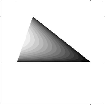
Figure 4: The dimensionless area $a_{H}$ as a function of $j_{\psi}$ and $j_{\phi}$ for fixed $\eta=0.4$. Note that the third dipole charge is not held constant, but is determined by the other parameters. Darker regions correspond to smaller area. On the left, the triangular region is bounded by the line $j_{\phi}=j_{\psi}$. The lower bound is a consequence of $j_{\phi}$ being bounded from below for non-vanishing dipole moment: $2\sqrt{2}\,j_{\phi}\geq\eta$. The region is bounded on the right by the line determined by $j_{\psi}^{\mathrm{max}}$ in (5.5). This is a consequence of requiring that there are no naked CCCs. The area $a_{H}$ vanishes at the bottom and right boundaries of the triangular region. For fixed $j_{\phi}$, $a_{H}$ is maximized when $j_{\psi}\to j_{\phi}$.

The expression (5.4) for the horizon area $a_{H}$ illustrates the non-uniqueness: the net charges are fixed and even when both the angular momenta are specified, we can still vary $\eta$. In particular, we can fix $j_{\psi}$ and $j_{\phi}$, and plot the entropy $a_{H}$ as a function of $\eta$. More generally, we can include both $\eta_{1}$ and $\eta_{2}$. Then we can use one parameter to fix the horizon area $a_{H}$ and still have another parameter to vary. We conclude that for given net charges $Q_{i}$ and angular momenta $j_{\phi,\psi}$, there are infinitely many supersymmetric black rings with the same horizon area, except for the black ring that maximizes the area, which is unique. This might suggest to recover a notion of uniqueness, at least among supersymmetric black rings, by adding the condition that the solution have maximum entropy for given conserved asymptotic charges. We emphasize, however, that this additional requirement is absent from the traditional notion of black hole uniqueness, and is also known to be insufficient to distinguish between non-supersymmetric black rings and black holes of spherical topology [1].

Figure 5 illustrates the non-uniqueness of supersymmetric black rings. It shows for fixed values of $j_{\phi}$ and $j_{\psi}$ the horizon area $a_{H}$ as a function of the dipole parameters $\eta_{1}$ and $\eta_{2}$. The bounds of the covered region are set by the requirement that there be no naked CCCs.

Figure 5: Contour plots of the dimensionless area $a_{H}$ versus $\eta_{1}$ and $\eta_{2}$, for fixed values of $j_{\phi}$ and $j_{\psi}$. For all three plots $4\sqrt{2}\,j_{\psi}=2.1$, but $j_{\phi}$ varies for each case: from left to right $4\sqrt{2}\,j_{\phi}=0.7$, $1.$, $1.7$. The plots are symmetric in $\eta_{1}$ and $\eta_{2}$, and the darker regions correspond to smaller area. The regions for which the black rings exist are bounded by the condition that there be no naked CCCs. At this boundary, the area $a_{H}$ vanishes.

Now consider what happens when we uplift the supersymmetric black ring to a $D=10$ D1-D5-P supertube, as described in section 4. In the quantum theory, the net charges and dipoles are quantized in terms of the number of branes in the D1-D5-P configuration. Using (4.4) and (4.5), we find that the restrictions (2.8) on the net charges $Q_{i}$ and dipole moments $q_{i}$ become

$$N_{\mathrm{D5}}\geq n_{\mathrm{D5}}\,n_{\mathrm{KK}}\,,\quad N_{\mathrm{D1}}\geq n_{\mathrm{D1}}\,n_{\mathrm{KK}}\,,\quad N_{\mathrm{P}}\geq n_{\mathrm{D1}}\,n_{\mathrm{D5}}\,.$$ (5.6)

So the number of D1- and D5-branes and units of momenta restrict the number of dipole branes and KK monopoles. This shows that upon quantization of the charges, the non-uniqueness becomes finite (but still very large).

6 Particular cases and limits

In this section we study various limits of the supersymmetric black ring solution. First in subsection 6.1, we consider the limit $R\to 0$ where the solution reduces to the BMPV black hole. In the infinite radius limit $R\to\infty$, the black ring becomes a black string in five dimensions. We show in subsection 6.2 that in this limit our solution reproduces the black string metric found in [16]. Subsection 6.3 contains special cases of the general black ring solution: one is the original two-charge supertube solution [6, 7], the other the three-charge solution with only two nonzero dipole moments. Finally, in subsection 6.4, we study the decoupling limit relevant for the AdS/CFT correspondence.

6.1 BMPV black hole

Consider the solution in the $(\rho,\Theta)$ coordinates of (3.1)–(3.3). If we set $R=0$ we find $H_{i}=1+Q_{i}/\rho^{2}$ and

$$\omega_{\phi}=-\frac{4G_{5}J}{\pi}\frac{\cos^{2}{\Theta}}{\rho^{2}}\,,~{}~{}~{}~{}\omega_{\psi}=-\frac{4G_{5}J}{\pi}\frac{\sin^{2}{\Theta}}{\rho^{2}}\,,~{}~{}~{}~{}A^{i}=H_{i}^{-1}(dt+\omega)\,,$$ (6.1)

where

$$J=\frac{\pi}{8G_{5}}\left[q_{1}Q_{1}+q_{2}Q_{2}+q_{3}Q_{3}-q_{1}q_{2}q_{3}\right]\,.$$ (6.2)

This is the BMPV black hole with three independent charges $Q_{i}$ and angular momenta $J_{\psi}=J_{\phi}=J$ [19]. Note that the parameters $q_{i}$ have become redundant since they enter the solution only through the angular momentum $J$. In particular, they no longer appear in $A^{i}$ and therefore no longer have the interpretation of dipole charges. The horizon is located at $\rho\to 0$. Topologically the horizon is a three-sphere. The horizon area is

$$\mathcal{A}_{\mathrm{BMPV}}=2\pi^{2}\sqrt{Q_{1}Q_{2}Q_{3}-\left(\frac{4G_{5}J}{\pi}\right)^{2}}\,.$$ (6.3)

This is not the $R\to 0$ limit of the horizon area of the supersymmetric black ring (3.30),

$$\lim_{R\to 0}\mathcal{A}_{\mathrm{ring}}=2\pi^{2}\sqrt{Q_{1}Q_{2}Q_{3}-\mathcal{Q}_{1}\mathcal{Q}_{2}\mathcal{Q}_{3}-\left(\frac{4G_{5}J}{\pi}\right)^{2}}\,,$$ (6.4)

which is always smaller than that of the BMPV black hole with the same asymptotic charges, except possibly when both areas vanish. The areas are compared in fig. 6 for the particular case of equal charges $Q_{i}=Q$ and dipoles $q_{i}=q$, i.e., for the solutions of minimal supergravity.

Figure 6: Area of the BMPV black hole (dashed) and limit $R\to 0$ of the area of the supersymmetric black ring (solid), vs. spin², for fixed mass (in terms of the variables $a_{H}$ and $j$ in (5.1)). For simplicity the three charges and dipoles are set equal, $Q_{i}=Q$, $q_{i}=q$ so these are solutions of minimal $D=5$ supergravity.

A clue to a (macroscopic) understanding of this effect follows by considering an analogy to a two-center extremal Reissner-Nordstrom (RN) solution. Observe that if we take a diameter section of the black ring solution, at constant $\psi$ and $\psi+\pi$, then the resulting four-dimensional geometry contains two infinite throats and therefore is similar to the geometry of two extremal black holes. The limit in which the inner radius of the ring shrinks to zero is in this sense analogous to the process in which the two centers of the extremal black holes are taken to coincide. If two RN extremal black holes, each of charge $Q$, are separate, the total mass is $2Q$ and the total area is $2(4\pi Q^{2})$. When their centers coincide the mass is still $2Q$ but the entropy jumps to $4\pi(2Q)^{2}$. So the limit of zero separation is discontinuous, and indeed the topology of the solution changes. This same effect occurs for the black ring: the area of the solution with $R=0$, i.e., the BMPV black hole, is larger than the limit $R\to 0$ of the ring area, and the topology of the two solutions are different.

6.2 Infinite radius limit

In this limit we take $R\to\infty$, but keep the charges per unit length along the tube ($2\pi R$) finite by defining finite linear densities (the factors $\Omega_{n}$ account for different dimensionalities of spheres for integration)

$${\bar{Q}_{i}}=\frac{Q_{i}}{2\pi R}\frac{2\Omega_{3}}{\Omega_{2}}=\frac{Q_{i}}{2R}$$ (6.5)

We keep $q_{i}$ fixed and define finite coordinates $\bar{r}$, $\bar{\theta}$, $\eta$ by

$$\bar{r}=-R/y\,,\quad\cos\bar{\theta}=x\,,\quad\eta=R\psi\,.$$ (6.6)

Then we get

$$H_{1} \to 1+\frac{\bar{Q}_{1}}{\bar{r}}+\frac{q_{2}q_{3}}{4\bar{r}^{2}}\,,$$ (6.7)

$$\omega_{\psi}d\psi \to -\left(\frac{q_{1}+q_{2}+q_{3}}{2\bar{r}}+\frac{q_{1}\bar{Q}_{1}+q_{2}\bar{Q}_{2}+q_{3}\bar{Q}_{3}}{4\bar{r}^{2}}+\frac{q_{1}q_{2}q_{3}}{8\bar{r}^{3}}\right)d\eta\,,$$ (6.8)

$$\omega_{\phi} \to 0\,,$$ (6.9)

with $H_{2}$ and $H_{3}$ given by permutations of (123). With this we reproduce the metric for the ‘flat supertube’ in [16].

6.3 Simpler supertubes

6.3.1 Two charges and one dipole

The original supergravity supertube solutions in $D=6$ [36, 37, 7] correspond to setting $Q_{3}=0$ and therefore $q_{1}=q_{2}=0$. In this case $J_{\phi}=0$ and $J_{\psi}=(\pi/4G_{5})R^{2}q_{3}$. The bound (3.25) is trivially saturated, but this inequality is only sufficient to eliminate CCCs when $q_{i}>0$. In the present case, it is easy to use the results of Appendix C to see that the necessary and sufficient condition for the absence of CCCs is $q_{3}^{2}\leq Q_{1}Q_{2}/R^{2}$, which agrees precisely with the worldvolume analysis of these supertubes in [6, 7].

6.3.2 Three charges and two dipoles

The solution with $q_{3}=0$ and $Q_{1,2,3}\neq 0$, $q_{1,2}\neq 0$, is more complicated than the previous one in that the BPS equations that it solves are non-linear and therefore the functions $H_{i}$ are not harmonic. There are also two independent angular momenta.

The solution can be interpreted as a helical D1-D5 string carrying momentum in the direction of the axis of the helix, along which it is smeared, but this time the KK monopole tube is absent. It is different than the D1-D5-P gyrating strings of [38], since it has two independent angular momenta and the area is always zero. In fact, now there is a naked curvature singularity at $y=-\infty$ where $R_{\mu\nu}R^{\mu\nu}$ diverges.

Absence of causal anomalies imposes again constraints on the parameters. Equation (3.25) reduces to $-(q_{1}Q_{1}-q_{2}Q_{2})^{2}\geq 0$ so we require

$$q_{1}Q_{1}=q_{2}Q_{2}\,.$$ (6.10)

In terms of quantized brane numbers (4.4), (4.5), this equation becomes

$$\frac{N_{\mathrm{D1}}}{n_{\mathrm{D1}}}=\frac{N_{\mathrm{D5}}}{n_{\mathrm{D5}}}\,,$$ (6.11)

which means that the D1 and D5 helices have the same pitch and can therefore bind to form a D1-D5 helix.

From Appendix C, it is now easy to see that the necessary and sufficient condition for absence of CCCs is that the radius $R$ be bounded above like

$$R^{2}\leq\frac{(Q_{3}-q_{1}q_{2})Q_{1}Q_{2}}{q_{1}q_{2}(Q_{1}+Q_{2})}\,.$$ (6.12)

Eq. (6.11) is the precise T-dual (in the $z$ direction) to a constraint found for supertubes with D0-D4-F1 charges and D2-D6 dipoles using the worldvolume theory of D6-branes [15]. Eq. (6.12) is very similar to, but not exactly the same as, another equation derived in [15] for the same system. We will return to this point in Sec. 8.

It is perhaps surprising that despite having the three D1-D5-P charges, the area of this solution always vanishes. The apparent reason is that near the core at $y\to-\infty$ the solution is mostly dominated by terms involving the dipole moments $q_{i}$. There is a curvature singularity at the core and the moduli also blow up there. However, it will be shown in [39] that this solution admits thermal deformations, i.e., there exists a family of non-extremal solutions with regular horizons, which in the extremal limit reduce to the supersymmetric solution with three charges and two dipoles.

One can easily check that the solutions with three charges and one dipole, as well as the ones with two charges and two dipoles, always possess CTCs near $y\to-\infty$. This parallels the fact that these supertubes do not have a sensible Born-Infeld description [15, 16].

6.4 Decoupling limit

In the decoupling limit of the D1-D5-P solution we send $\alpha^{\prime}=\ell_{s}^{2}\to 0$ and keep the string coupling $g_{s}$ fixed, in such a way that the geometry near the core decouples from the asymptotically flat region. Our solution contains several more parameters than previous D1-D5-P configurations, so we shall describe this limit in some detail.

We work with the coordinates $(r,\theta)$ defined in (3.7). Since we want to keep fixed the energies (in string units) of the excitations that live near the core, then $r/\alpha^{\prime}$ and $R/\alpha^{\prime}$ must remain finite. We are also interested in a regime where the size of the $z$ direction, $R_{z}$, is large compared to $\ell_{s}$, so that winding modes can be ignored and the momentum modes are the lowest excitations. So when we take $\alpha^{\prime}\to 0$, $R_{z}$ will be fixed, and then also $q_{3}$ as a result of (4.8). Further, we take the $T^{4}$ length scale $\ell\sim\ell_{s}$ so that the energy scale of both momentum and winding modes on the $T^{4}$ is large. Finally, we keep the string coupling fixed and also keep the number of branes and units of momentum fixed. Using (4.4) and (4.5) the limiting solution is obtained taking $\alpha^{\prime}\to 0$ while

$$r/\alpha^{\prime}\,, \qquad Q_{1,2}/\alpha^{\prime}\,,\qquad Q_{3}/{\alpha^{\prime}}^{2}\,,$$

$$R/\alpha^{\prime}\,, \qquad q_{1,2}/\alpha^{\prime}\,,\qquad q_{3}\,$$ (6.13)

are held fixed. Then the length scales in the supergravity solution are arranged as

$$r\sim R\sim\sqrt{Q_{3}}\sim\sqrt{q_{1}q_{2}}\ll(Q_{1}Q_{2})^{1/4}\sim\sqrt{q_{3}}(q_{1}q_{2})^{1/4}$$ (6.14)

with $Q_{1}\sim Q_{2}$ and $q_{1}\sim q_{2}$. Recall from (4.1) that $Q_{1}$, $Q_{2}$, and $Q_{3}$ label D5, D1, and momentum charge, respectively, and $q_{1}$, $q_{2}$, and $q_{3}$ correspond to the dipole charges of respectively d1- and d5-branes and the Kaluza-Klein monopoles making up the supertube. Observe also that $\mathcal{Q}_{i}$ scales like $Q_{i}$.

After rescaling the metric and the gauge fields $A^{1}$ and $A^{2}$ by an overall factor of $\alpha^{\prime}$, we obtain a new solution of IIB supergravity. This decoupled solution has the same form as (4.2), (4.3), (2) with, in the coordinates of (3.8),

$$H_{1,2} = \frac{Q_{1,2}}{\Sigma}-\frac{q_{2,1}q_{3}R^{2}\cos 2\theta}{\Sigma^{2}}\,,$$

$$H_{3} = 1+\frac{Q_{3}}{\Sigma}-\frac{q_{1}q_{2}R^{2}\cos 2\theta}{\Sigma^{2}}\,,$$ (6.15)

$$\omega_{\psi} = -q_{3}\frac{R^{2}\sin^{2}\theta}{\Sigma}-\frac{(r^{2}+R^{2})\sin^{2}{\theta}}{\Sigma^{2}}\left(\frac{4G_{5}J_{\phi}}{\pi}-q^{3}\frac{R^{2}\cos 2\theta}{\Sigma}\right)\,.$$

while $\omega_{\phi}$ and $A^{i}$ remain as in (3.11) and (3.12), and $J_{\phi}$ is as in (3.13). We can gauge-transform $A^{3}\to A^{3}-dt$, i.e., $z\to z-t$, so that $A^{3}_{t}=H_{3}^{-1}-1$ vanishes at $r\to\infty$. It is apparent that this decoupling limit amounts to the familiar procedure of “removing the 1’s” from the functions $H_{1,2}$ associated to the D5 and D1 branes, with the first term of $\omega_{\psi}$ modified so the result remains a solution of the field equations.

The decoupling limit is not in general the same as the near-horizon limit (4.2.2) analyzed earlier. In the near-horizon limit $r$ is taken to be much smaller than $R$ and indeed than any other scale in the system, so one covers only a small region of the decoupled solution. Also, the near-horizon limit in (4.2.2) exists for any black ring, whereas here we are restricting the parameters to the ranges in (6.14). These differences between the two limits are in fact also present for BMPV [40]. The two limits nevertheless commute, so the new solution has a regular horizon of finite area. After an appropriate rescaling, $L$ is the same as (3.28), when expressed in terms of physical quantities only. A slight difference is hidden, though, in the fact that in the decoupling limit $J_{\psi}-J_{\phi}$ changes to

$$(J_{\psi}-J_{\phi})_{\rm{decoupled}}=\frac{\pi}{4G_{5}}R^{2}q_{3}\,.$$ (6.16)

This is simply a consequence of the restrictions (6.13) on the relative values of the parameters, which imply in particular that $q_{3}\gg q_{1,2}$. As a consequence, rings with $q_{3}\sim q_{1,2}$ are not expected to be fully captured by the dual CFT description of D1-D5 systems.

At asymptotic infinity, $r\to\infty$, the metric becomes (omitting the $T^{4}$ factor)

$$ds^{2}\to\frac{r^{2}}{\sqrt{Q_{1}Q_{2}}}(-dt^{2}+dz^{2})+\sqrt{Q_{1}Q_{2}}\;\frac{dr^{2}}{r^{2}}+\sqrt{Q_{1}Q_{2}}(d\theta^{2}+\sin^{2}\theta d\psi^{2}+\cos^{2}\theta d\phi^{2})\,,$$ (6.17)

so we recover the asymptotic geometry of global (as $z$ is periodic) AdS₃ times $S^{3}$, both with equal radius

$$\ell_{\infty}=(Q_{1}Q_{2})^{1/4}\,.$$ (6.18)

For certain particular values of the parameters we get solutions which are everywhere locally AdS${}_{3}\times S^{3}$. This happens when $R=0$, i.e., BMPV in the decoupling limit [40], and also for two-charge D1-D5 supertubes that saturate the CTC bound $q_{3}^{2}R^{2}=Q_{1}Q_{2}$. The decoupling limit of the latter is global AdS₃ times a rotating $S^{3}$, with a conical singularity if $n_{\mathrm{KK}}>1$ [36].

However, in general our solution is (locally) the product space AdS${}_{3}\times S^{3}$ only at asymptotic infinity and near the horizon. In the latter region this occurs in a rather unusual manner. In order to find the near-horizon limit of the decoupling solution in $(r,\theta)$ coordinates, near $r=0$, $\theta=\pi/2$, we take the gauge in which $A^{3}_{t}=H_{3}^{-1}$ so we are in a frame that corotates with the horizon, and define

$$r^{2}=\epsilon\tilde{r}L\cos^{2}\frac{\tilde{\theta}}{2}\,,\qquad R^{2}\cos^{2}\theta=\epsilon\tilde{r}L\sin^{2}\frac{\tilde{\theta}}{2}\,,\qquad t=\tilde{t}/\epsilon\,.$$ (6.19)

Sending $\epsilon\to 0$, the geometry that results is the same as (4.2.2), but now in coordinates that cover only the region outside the horizon,

$$ds^{2} = \frac{2L}{\sqrt{q_{1}q_{2}}}\,\tilde{r}\,d\tilde{t}\,d\psi+\frac{qL^{2}}{\sqrt{q_{1}q_{2}}}\,d{\psi}^{2}+\frac{q_{3}\sqrt{q_{1}q_{2}}}{4}\frac{d\tilde{r}^{2}}{\tilde{r}^{2}}$$

$$+\frac{\sqrt{q_{1}q_{2}}}{q_{3}}\left(dz-\frac{q_{3}}{2}(1+\cos\tilde{\theta})d\chi\right)^{2}+\frac{q_{3}\sqrt{q_{1}q_{2}}}{4}\left(d{\tilde{\theta}}^{2}+\sin^{2}\tilde{\theta}d\chi^{2}\right)\,,$$

where we use $\chi=\phi-\psi$ and, for simplicity, we assume (4.11) is satisfied so that we can use a shift $z\to z+m\,R_{z}\psi$ to bring the geometry to a product of two factors. The first factor is locally isometric to AdS₃ with radius

$$\ell_{\mathrm{nh}}=\sqrt{q_{3}}(q_{1}q_{2})^{1/4}\,.$$ (6.21)

This factor is globally the same as the near-horizon limit of an extremal BTZ black hole with mass and spin

$$M_{\mathrm{BTZ}}=2L^{2}/q^{2}\,,\qquad J_{\mathrm{BTZ}}=M_{\mathrm{BTZ}}\ell_{\mathrm{nh}}\,,$$ (6.22)

and horizon at $\tilde{r}=0$. The second factor is the quotient space $S^{3}/Z_{n_{\mathrm{KK}}}$, with the same radius $\ell_{\mathrm{nh}}$.

The appearance of AdS${}_{3}\times S^{3}$ near the horizon is very different from the factorization into AdS${}_{3}\times S^{3}$ in the asymptotic region (6.17). The AdS₃ near the horizon spans the coordinates $(\tilde{t},\tilde{r},\psi)$ whereas near the asymptotic boundary it spans $(t,r,z)$ —the relation between $t$ and $\tilde{t}$ just amounts to the redshift near the horizon, but the other coordinates are not simply related.

The direction in which the near-horizon geometry rotates is $\psi$. In contrast, in the decoupling limit of BMPV, the near-horizon geometry rotates in the $z$-direction and arises from the linear momentum in this direction. Here the rotation of the near-horizon geometry arises, in a sense, from the rotation of the ring, but there is no simple relationship between $J_{\psi}$ and $J_{\mathrm{BTZ}}$. Furthermore, the radii of the two AdS₃’s are different

$$\ell_{\infty}>\ell_{\mathrm{nh}}.$$ (6.23)

The curvature of the solution near the horizon is not controlled by the net D1 and D5 charges but instead by the dipole charges $q_{i}$. As a consequence, the simple argument for the statistical calculation of the entropy of the BTZ black hole, from the charges under the Virasoro algebra of diffeomorphisms at the boundary of AdS₃ [41], does not seem to apply easily to the computation of the entropy of the ring.

So the full decoupling solution interpolates in a highly non-trivial way between two different factorizations of the six-dimensional solution, both of which are locally of the form AdS${}_{3}\times S^{3}$. Between these two limiting regions, the solution has non-vanishing Weyl curvature and is generically quite complicated. Indeed, already when the first subleading terms near $r\to\infty$ are considered, the geometry does not factorize.

This decoupled solution must admit a dual description in terms of an ensemble of supersymmetric states of the dual CFT. It should be very interesting to identify and count the degeneracy of these states to reproduce the entropy of the black ring. Given the two limiting AdS geometries, it might be useful to view the solution as dual to a renormalization group flow, with equation (6.23) implying that the central charge is greater in the UV than in the IR, as expected from the $c$-theorem.

7 Worldvolume Supertubes and Kähler Calibrations

Consider three M5-branes intersecting as in the array (2.1), with the $\psi$-circle replaced by a curve $C$ in the ${\mathbb{E}}^{4}$ space transverse to the M2-branes. If $C$ is a straight line, then the worldspace of the three M5-branes may be described as that of a single M5-brane with (in general) non-singular worldspace $S\times C$, where $S$ is a Kähler-calibrated surface of degree four (that is, of complex dimension two) embedded in the $\mbox{${\mathbb{C}}^{3}$}=\mbox{${\mathbb{E}}^{6}$}$ space spanned by the $z^{1},\ldots,z^{6}$ coordinates. This configuration preserves 1/8 of the thirty-two supersymmetries of the M-theory Minkowski vacuum. Here we will show that an M5-brane with worldspace $S\times C$ and appropriate fluxes of the worldvolume three-form $H$ also preserves 1/8 of the supersymmetries (albeit a different set) for any arbitrary curve $C$ in ${\mathbb{E}}^{4}$. If $C$ is closed then this configuration carries no net M5-brane charges, but only three M2-brane charges and three M5-brane dipoles, and thus provides the first worldvolume description of a three-charge supertube in which the three dipoles are visible. We call this a calibrated supertube. In fact, we will show that any Kähler calibration (of appropriate degree to be interpreted in terms of M5-branes) gives rise to a calibrated supertube in a similar manner. It would be interesting to investigate the relationship between supertubes and other types of calibrations (SLAG calibrations, exceptional calibrations, etc..), with calibrations in more general backgrounds, and with calibrations corresponding to non-static branes.

To avoid any confusion, it is worth mentioning from the start a limitation of the worldvolume description we are about to present. This is the fact that, although the configurations we will construct do carry multiple charges and dipoles globally, they may be locally regarded as standard two-charge/one-dipole supertubes. Globally, therefore, they may be viewed as resolved junctions of standard supertubes, in the same sense that certain calibrations can be viewed as resolved junctions of M5-branes. One very concrete manifestation of this limitation is that the worldvolume description does not capture the second angular momentum visible in the supergravity description.

Despite this limitation, it is remarkable that such non-singular junctions of supertubes can preserve supersymmetry, and we regard the construction below as a first step towards a more sophisticated worldvolume description of three-charge black supertubes.

7.1 Kähler calibrations and intersecting M5-branes

We begin by reviewing a few facts about Kähler calibrations. We follow closely the discussion in [43, 44]. Let $u^{j}=z^{2j-1}+iz^{2j}$, with $j=1,\ldots,n$, be complex coordinates on $\mbox{${\mathbb{C}}^{n}$}=\mbox{${\mathbb{E}}^{2n}$}$, with metric

$$ds^{2}=\sum_{j=1}^{n}du^{j}\,d\bar{u}^{j}=\sum_{j=1}^{2n}dz_{j}^{2}\,,$$ (7.1)

and

$$\mbox{${\cal H}$}=\frac{i}{2}\sum_{j=1}^{n}du^{j}\wedge d\bar{u}^{j}=\sum_{j=1}^{n}dz^{2j-1}\wedge dz^{2j}$$ (7.2)

the associated Kähler two-form. Then

$$\Psi=\frac{1}{p!}\,\mbox{${\cal H}$}^{p}$$ (7.3)

is a calibration of degree $2p$ in ${\mathbb{C}}^{n}$ ($p\leq n$) associated to the group $SU(n)$ [45]. This means that the volume of any (hyper)surface $S\subset\mbox{${\mathbb{E}}^{2n}$}$ of dimension $2p$ is bounded from below as

$$\int_{S}d^{2p}\xi\,\sqrt{\det g}\geq\int_{S}\,\Psi\,,$$ (7.4)

where $\xi$ are coordinates on $S$, $g$ is the induced metric on $S$, and a pull-back of $\Psi$ onto $S$ is understood. If this bound is saturated, the surface $S$ is said to be calibrated by $\Psi$, or Kähler calibrated (since $\Psi$ is constructed from the Kähler form). All complex surfaces in ${\mathbb{C}}^{n}$ are Kähler calibrated [43]. Since $S$ minimizes its volume within its homology class, a static M5-brane with worldspace $S\times\mbox{${\mathbb{E}}^{5-2p}$}$ is a solution of the M5-brane equations of motion. Moreover, any two tangent (hyper)planes to $S$ are related by an $SU(n)\subset SO(2n)$ rotation, from which it follows that a fraction $1/2^{n}$ of supersymmetry is preserved.

The Kähler calibrations of interest here are those that have an interpretation in terms of intersecting M5-branes, namely those with $n=2,3,4$. For $n=2$ there is only an $SU(2)$ calibration of degree two, corresponding to a Riemann surface $S$ embedded in ${\mathbb{C}}^{2}$. An M5-brane with worldspace $S\times\mbox{${\mathbb{E}}^{3}$}$ can be interpreted as the intersection of two M5-branes

$$\begin{array}[]{rcccccccl}\mbox{M5:}&1&2&\_&\_&5&6&7&\\ \mbox{M5:}&\_&\_&3&4&5&6&7&\,,\end{array}$$ (7.5)

where the ${\mathbb{C}}^{2}$ space corresponds to the 1234-directions.

For $n=3$ there are two relevant calibrations, of degrees two and four. The first one corresponds to a Riemann surface $S$ in ${\mathbb{C}}^{3}$. An M5-brane with worldspace $S\times\mbox{${\mathbb{E}}^{3}$}$ preserves 1/8-supersymmetry and can be interpreted as describing the triple intersection

$$\begin{array}[]{rcccccccccl}\mbox{M5:}&1&2&\_&\_&\_&\_&7&8&9&\\ \mbox{M5:}&\_&\_&3&4&\_&\_&7&8&9&\\ \mbox{M5:}&\_&\_&\_&\_&5&6&7&8&9&\,.\end{array}$$ (7.6)

The $SU(3)$ calibration of degree four corresponds to a surface $S$ of complex dimension two embedded in ${\mathbb{C}}^{3}$. An M5-brane with worldspace $S\times\mbox{${\mathbb{E}}$}$ can be interpreted as the triple intersection

$$\begin{array}[]{rcccccccl}\mbox{M5:}&\_&\_&3&4&5&6&7&\\ \mbox{M5:}&1&2&\_&\_&5&6&7&\\ \mbox{M5:}&1&2&3&4&\_&\_&7&\,.\end{array}$$ (7.7)

In both $SU(3)$ cases, the ${\mathbb{C}}^{3}$ space corresponds to the 123456-directions. As mentioned above, the second case corresponds to the M5 intersection in (2.1) with the circle replaced by a line.

Finally, the only $SU(4)$ calibration that has an interpretation in terms of M5-branes is that of degree four, which corresponds to a surface $S$ of complex dimension two embedded in ${\mathbb{C}}^{4}$. An M5-brane with worldspace $S\times\mbox{${\mathbb{E}}$}$ can be interpreted as the sixtuple intersection

$$\begin{array}[]{rcccccccccl}\mbox{M5:}&1&2&3&4&\_&\_&\_&\_&9&\\ \mbox{M5:}&1&2&\_&\_&5&6&\_&\_&9&\\ \mbox{M5:}&1&2&\_&\_&\_&\_&7&8&9&\\ \mbox{M5:}&\_&\_&3&4&5&6&\_&\_&9&\\ \mbox{M5:}&\_&\_&3&4&\_&\_&7&8&9&\\ \mbox{M5:}&\_&\_&\_&\_&5&6&7&8&9&\,.\end{array}$$ (7.8)

Although in all arrays above we have displayed the M5-branes as being orthogonal, this need not be the case; they can intersect at arbitrary $SU(n)$ angles, which are encoded in $S$. Let us illustrate this for the $SU(3)$ calibration of degree four, represented by (7.7). The surface $S$ can generally be specified as the locus $F(u_{1},u_{2},u_{3})=0$, where $F$ is a holomorphic function. The choice of $F$ determines the $SU(3)$ angles between the three M5-branes, which arise at asymptotic regions of $S$. As an example, consider $F=f_{1}f_{2}f_{3}-c$, where $f_{i}=\sum_{j=1}^{3}a_{i}^{j}\,u^{j}$ are linear functions and $a_{i}^{j}$ and $c$ are constants. The induced metric on $S$ has three asymptotically flat regions that can be identified with the three M5-branes. A simple way to determine these is to set $c=0$. In this case the locus $F=0$ consists of three complex planes, $f_{1}=0$, $f_{2}=0$ and $f_{3}=0$, the angles between them being determined by the constants $a_{i}^{j}$. This corresponds to a singular intersection of three M5-branes that extend along these three planes. Setting now $c\neq 0$ smooths out the intersection and hence allows the entire complex two-surface to be interpreted as a single M5-brane, but does not alter the orientations of the asymptotic regions, which therefore can still be identified with three distinct M5-branes.

Despite the fact that the arrays above do not necessarily specify the $SU(n)$ angles between the intersecting branes, each array is useful in summarizing the number of participating branes and the set of supersymmetries preserved by each intersection. For example, the configuration represented by the array (7.5) preserves 1/4-supersymmetry, corresponding to the Killing spinors $\eta$ subject to the constraints

$$\Gamma_{012567}\,\eta=\eta\,,\qquad\Gamma_{034567}\,\eta=\eta\,,$$ (7.9)

each of them being associated to one of the M5-branes. Similarly, the configuration represented by (7.8) preserves 1/16-supersymmetry, corresponding to any four of the six M5-branes (the two projectors associated to any two of the M5-branes are implied by the those of the other four).

7.2 Calibrated supertubes

We are now in a position to show that each of the Kähler calibrations above gives rise, through turning on appropriate worldvolume fluxes, to a calibrated supertube. Choosing $S=\mbox{${\mathbb{E}}^{2}$}\times S^{\prime}$, with $S^{\prime}$ a Riemann surface, in the $SU(3)$ and $SU(4)$ calibrations of degree four, represented by the arrays (7.8) and (7.7), we recover the $SU(2)$ and $SU(3)$ calibrations of degree two, represented by the arrays (7.5) and (7.6), respectively. The two degree-two calibrations can therefore be regarded as ‘degenerate’ cases of the two degree-four calibrations, and for this reason we will only discuss the latter two. These give rise to the three-charge/three-dipole $SU(3)$ calibrated supertube

$$\begin{array}[]{rcccccccl}Q_{1}\,\,\mbox{M2:}&1&2&\_&\_&\_&\_&\_&\\ Q_{2}\,\,\mbox{M2:}&\_&\_&3&4&\_&\_&\_&\\ Q_{3}\,\,\mbox{M2:}&\_&\_&\_&\_&5&6&\_&\\ q_{1}\,\,\mbox{m5:}&\_&\_&3&4&5&6&\sigma&\\ q_{2}\,\,\mbox{m5:}&1&2&\_&\_&5&6&\sigma&\\ q_{3}\,\,\mbox{m5:}&1&2&3&4&\_&\_&\sigma&\\ \end{array}$$ (7.10)

and to the four-charge/six-dipole $SU(4)$ calibrated supertube

$$\begin{array}[]{rcccccccccl}Q_{1}\,\,\mbox{M2:}&1&2&\_&\_&\_&\_&\_&\_&\_&\\ Q_{2}\,\,\mbox{M2:}&\_&\_&3&4&\_&\_&\_&\_&\_&\\ Q_{3}\,\,\mbox{M2:}&\_&\_&\_&\_&5&6&\_&\_&\_&\\ Q_{4}\,\,\mbox{M2:}&\_&\_&\_&\_&\_&\_&7&8&\_&\\ q_{1}\,\,\mbox{m5:}&1&2&3&4&\_&\_&\_&\_&\sigma&\\ q_{2}\,\,\mbox{m5:}&1&2&\_&\_&5&6&\_&\_&\sigma&\\ q_{3}\,\,\mbox{m5:}&1&2&\_&\_&\_&\_&7&8&\sigma&\\ q_{4}\,\,\mbox{m5:}&\_&\_&3&4&5&6&\_&\_&\sigma&\\ q_{5}\,\,\mbox{m5:}&\_&\_&3&4&\_&\_&7&8&\sigma&\\ q_{6}\,\,\mbox{m5:}&\_&\_&\_&\_&5&6&7&8&\sigma&\,.\end{array}$$ (7.11)

In the two arrays above, we have denoted by $\sigma$ the coordinate along the curve $C$. Note that each M5-brane can be thought of as originating from the expansion of a pair of M2-branes, as in a ‘standard’ two-charge supertube.

Consider therefore an M5-brane with worldspace $S\times C$, where $S$ is a complex two-surface in ${\mathbb{C}}^{3}$ or ${\mathbb{C}}^{4}$ and $C$ is an arbitrary curve in ${\mathbb{E}}^{4}$ or ${\mathbb{E}}^{2}$, with a worldvolume three-form flux $H=dB_{2}$ given by

$$H=d\sigma\wedge\mbox{${\cal H}$}+dx^{0}\wedge\mbox{${\cal H}$}^{\prime}\,,$$ (7.12)

where again ${\cal H}$ is understood to be pulled-back onto the M5-brane worldvolume. $\mbox{${\cal H}$}^{\prime}$ is a two-form determined in terms of ${\cal H}$ by the (generalized) self-duality condition satisfied by $H$, but whose explicit expression will not be needed. Closure of $H$ follows from that of ${\cal H}$. As we will see below, this $H$-flux induces M2-brane charges on the M5-brane as in the arrays (7.10) or (7.11). We claim that this configuration preserves 1/8 or 1/16 of the supersymmetries of the M-theory Minkowski vacuum, generated by Killing spinors $\eta$ subject to the constraints associated to the M2-branes, that is,

$$\Gamma_{012}\,\eta=\eta\,,\qquad\Gamma_{034}\,\eta=\eta\,,\qquad\Gamma_{056}\,\eta=\eta$$ (7.13)

for the three-charge supertube, and

$$\Gamma_{012}\,\eta=\eta\,,\qquad\Gamma_{034}\,\eta=\eta\,,\qquad\Gamma_{056}\,\eta=\eta\,,\qquad\Gamma_{078}\,\eta=\eta$$ (7.14)

for the four-charge supertube. Note that there is no trace of a condition associated to the M5-branes, as expected from the absence of M5-brane net charges.

To prove this, it is convenient to adopt a (static) gauge in which $x^{0}$, $x^{a}=(x^{1},\ldots,x^{4})$, and $\sigma$ are worldvolume coordinates on the M5-brane, where $\sigma$ parametrizes the cross-section $C$, specified as $x^{\mu}=x^{\mu}(\sigma)$. For the three-charge supertube $x^{\mu}=(x^{7},\ldots,x^{10})$, whereas for the four-charge supertube $x^{\mu}=(x^{9},x^{10})$. Without loss of generality we choose $\sigma$ to be the affine parameter along $C$, that is, $\delta_{\mu\nu}\,\partial_{\sigma}x^{\mu}\partial_{\sigma}x^{\nu}=1$. The complex surface $S$ is specified as $x^{m}=x^{m}(x^{a})$, where $x^{m}=(x^{5},x^{6})$ for the three-charge supertube and $x^{m}=(x^{5},\ldots,x^{8})$ for the four-charge supertube. In both cases, $x^{m}$ satisfy the appropriate Cauchy-Riemann equations,

$$\partial_{1}x^{5}=\partial_{2}x^{6}\,,\qquad\partial_{2}x^{5}=-\partial_{1}x^{6}\,,\qquad\ldots$$ (7.15)

where the dots stand for the same expression with $\{1,2\}$ and/or $\{5,6\}$ replaced by $\{3,4\}$ and/or $\{7,8\}$. Note that in these coordinates the only non-zero components of ${\cal H}$ are

$$\mbox{${\cal H}$}_{ab}=\delta_{1[a}\,\delta_{b]2}+\delta_{3[a}\,\delta_{b]4}+\partial_{[a}x^{5}\partial_{b]}x^{6}$$ (7.16)

for the three-charge supertube, and

$$\mbox{${\cal H}$}_{ab}=\delta_{1[a}\,\delta_{b]2}+\delta_{3[a}\,\delta_{b]4}+\partial_{[a}x^{5}\partial_{b]}x^{6}+\partial_{[a}x^{7}\partial_{b]}x^{8}$$ (7.17)

for the four-charge supertube. In both cases, the induced metric on the M5-brane worldvolume takes the form

$$ds^{2}=-dx_{0}^{2}+d\sigma^{2}+g_{ab}\,dx^{a}\,dx^{b}\,,$$ (7.18)

where

$$g_{ab}=\delta_{ab}+\partial_{a}x^{m}\,\partial_{b}x^{n}\,\delta_{mn}\,.$$ (7.19)

The number of supersymmetries of the Minkowski vacuum preserved by the M5-brane is the number of Killing spinors $\eta$ that satisfy the condition $\Gamma_{\mathrm{M5}}\,\eta=\eta$ [46], where $\Gamma_{\mathrm{M5}}$ is the matrix appearing in the kappa-symmetry transformations of the M5-brane worldvolume fermions. We work with a unit-tension M5-brane and the covariant formulation of [47], which contains an auxiliary scalar field $a$ that we eliminate by the gauge choice $a=x^{0}$. Under these circumstances the kappa-symmetry matrix takes the same form for the three- and four-charge supertubes, namely,

$$\Gamma_{\mathrm{M5}}=\frac{\Gamma_{0}}{\sqrt{\det(g_{ab}+h_{ab})}}\,\left[\frac{1}{4}\,\epsilon^{abcd}\,\mbox{${\cal H}$}_{ab}\,\gamma_{cd}-\gamma_{\sigma}\,\left(\mbox{${\cal P}$}_{\sigma}+\gamma_{1234}\right)\right]\,,$$ (7.20)

where $\epsilon^{1234}=+1$,

$$\gamma_{a}=\Gamma_{a}+\partial_{a}x^{m}\,\Gamma_{m}\,,\qquad\gamma_{\sigma}=\partial_{\sigma}x^{\mu}\,\Gamma_{\mu}$$ (7.21)

are the worldvolume Dirac matrices induced by the spacetime, constant Dirac $\Gamma$-matrices, $\gamma_{i_{1}\ldots i_{n}}=\gamma_{[i_{1}}\gamma_{i_{2}}\cdots\gamma_{i_{n}]}$,

$$\mbox{${\cal P}$}_{\sigma}=\frac{1}{8}\,\epsilon^{abcd}\,\mbox{${\cal H}$}_{ab}\,\mbox{${\cal H}$}_{cd}$$ (7.22)

is the momentum density along $\partial_{\sigma}$, and

$$h_{ab}\equiv\frac{1}{2}\,g_{ac}\,g_{bd}\,\frac{\epsilon^{cdef}}{\sqrt{\det g}}\,\mbox{${\cal H}$}_{ef}\,.$$ (7.23)

Making use of (7.13), (7.14), (7.15), (7.16) and (7.17), a tedious but straightforward calculation reveals that

$$\gamma_{1234}\,\eta=-\mbox{${\cal P}$}_{\sigma}\,\eta\,,$$ (7.24)

where

$$\mbox{${\cal P}$}_{\sigma}=1+\delta^{ab}\,\partial_{a}x^{6}\,\partial_{b}x^{6}$$ (7.25)

for the three-charge supertube, and

$$\mbox{${\cal P}$}_{\sigma}=1+\delta^{ab}\,\partial_{a}x^{6}\,\partial_{b}x^{6}+\delta^{ab}\,\partial_{a}x^{8}\,\partial_{b}x^{8}+\epsilon^{abcd}\,\partial_{a}x^{5}\,\partial_{b}x^{6}\,\partial_{c}x^{7}\,\partial_{d}x^{8}$$ (7.26)

for the four-charge supertube. We note that the Cauchy-Riemann equations imply $\delta^{ab}\,\partial_{a}x^{5}\,\partial_{b}x^{5}=\delta^{ab}\,\partial_{a}x^{6}\,\partial_{b}x^{6}$, and analogously with $\{5,6\}$ replaced by $\{7,8\}$.

It follows that the two terms inside the round brackets in (7.20) cancel each other, and hence all information about the cross-section $C$, which is entirely encoded in $\gamma_{\sigma}$, drops from the supersymmetry equation. This now reduces to

$$\frac{1}{4}\,\epsilon^{abcd}\,\mbox{${\cal H}$}_{ab}\,\Gamma_{0}\gamma_{cd}\,\eta=\sqrt{\det(g_{ab}+h_{ab})}\,\eta\,.$$ (7.27)

Using again (7.13), (7.14), (7.15), (7.16) and (7.17), one can verify that this equation is identically satisfied, with the determinant given by

$$\sqrt{\det(g_{ab}+h_{ab})}=2\,\sqrt{\det g_{ab}}=2\mbox{${\cal P}$}_{\sigma}\,.$$ (7.28)

Essentially the same arguments given above can be used to show that these supertube configurations saturate the bounds found in [48, 49]. It is worth remarking, though, that the configurations studied in detail in those references all have zero momentum density, i.e., $\mbox{${\cal P}$}_{\sigma}=\mbox{${\cal P}$}_{a}=0$.

7.3 Physical properties

In this section we will show that a calibrated supertube can be regarded, at a given point, as a standard supertube with one M5 dipole and two M2 charges. For the standard supertube, supersymmetry fixes both these densities and the shape of the tube in the directions transverse to the cross-section (i.e., it fixes $S$) [6]. For a calibrated supertube, stability is instead achieved locally in such a way that the only restriction on this shape is that $S$ be a calibrated surface; the charge densities may then also vary, as they are given by the pull-back onto $S$ of the Kähler form. This allows the calibrated supertube to carry, globally, more than two net charges and one dipole, as we have seen above. In this sense, the worldvolume three-charge supertube constructed in this paper may be regarded as a smooth junction of three two-charge supertubes associated to the three asymptotic regions of $S$.

The cross-section of the calibrated supertube, like that of the standard one, is supported against collapse by the ‘centrifugal force’ associated to the Poynting momentum density generated by the product of the worldvolume charge densities. To see this, we note that the momentum density $\mbox{${\cal P}$}_{\sigma}$ is, at each point, the product of the two M2-brane charge densities carried by the M5-brane at that point. Recall that the M2-brane charge density in the $ab$-directions tangent to a given point on the M5-brane is given by the momentum density $\Pi^{ab}$ conjugate to the worldvolume two-form potential $B_{ab}$. This is because the M5-brane action depends only on the background-covariant combination $H+\mathcal{A}$, where $H=dB_{2}$ and a pull-back onto the M5 worldvolume of the supergravity three-form potential $A$ is understood. It follows from this that the M2-brane charge density carried by the M5 is

$$\left.\frac{\partial\mbox{${\cal L}$}_{\mathrm{M5}}}{\partial\mathcal{A}_{0ab}}\right|_{\mathcal{A}=0}=\left.\frac{\partial\mbox{${\cal L}$}_{\mathrm{M5}}}{\partial\dot{B}_{ab}}\right|_{\mathcal{A}=0}=\Pi^{ab}\,.$$ (7.29)

This momentum is determined in terms of the worldspace components of $H$ by the constraint associated to the self-duality condition of $H$ [50]. In the present case it takes the form

$$\Pi^{ab}=\frac{1}{2}\,\epsilon^{abcd}\,\mbox{${\cal H}$}_{cd}\,,$$ (7.30)

so $\mbox{${\cal P}$}_{\sigma}$ may be rewritten as

$$\mbox{${\cal P}$}_{\sigma}=\frac{1}{8}\,\epsilon_{abcd}\,\Pi^{ab}\,\Pi^{cd}\,.$$ (7.31)

Now, at each point on $S$ an orthonormal basis of its tangent space may be chosen such that the antisymmetric tensor $\Pi^{ab}$ is skew-diagonal, with skew-eigenvalues $\Pi$ and $\Pi^{\prime}$. These measure the magnitude of the two independent M2-brane charge densities at the given point, whereas the orthonormal basis determines their orientations. In terms of these densities we have

$$\mbox{${\cal P}$}_{\sigma}=\Pi\,\Pi^{\prime}\,,$$ (7.32)

as anticipated.

Equation (7.32) is completely analogous to that for a two-charge standard supertube [6, 7]. We now show that the rest of the relations between the charge densities, the angular momentum and the size of the cross-section also are, at a given point, as those of the two-charge supertube. For simplicity, we assume that $C$ is a circle of radius $R$ in some plane, so we set $\sigma=R\,\psi$. It is important to remember that the densities that enter these relations are densities per unit area of $S$, obtained by normalizing by $\sqrt{\det g_{ab}}$ and integrating over $C$. The normalization is most easily accounted for by working in the orthonormal basis used to define $\Pi$ and $\Pi^{\prime}$, so that $\det g_{ab}=1$. By virtue of the second equality in (7.28), this implies

$$\mbox{${\cal P}$}_{\sigma}=\Pi\Pi^{\prime}=1\,,$$ (7.33)

as for the for the standard supertube [8]. The $C$-integrated M2-brane densities are

$$\varrho=\frac{1}{2\pi}\int_{C}d\sigma\,\Pi=R\,\Pi\,,\qquad\varrho^{\prime}=\frac{1}{2\pi}\int_{C}d\sigma\,\Pi^{\prime}=R\,\Pi^{\prime}\,,$$ (7.34)

where we have used the fact that $\sigma$ is the affine parameter along $C$ and that $\Pi,\Pi^{\prime}$ are $\sigma$-independent. It then follows from (7.33) that

$$R=\sqrt{\varrho\varrho^{\prime}}\,.$$ (7.35)

Similarly, the angular momentum is

$$J_{\psi}=\frac{R}{2\pi}\int_{C}d\sigma\,\mbox{${\cal P}$}_{\sigma}=R^{2}\,,$$ (7.36)

and hence

$$J=\varrho\varrho^{\prime}\,.$$ (7.37)

We thus see that $R$, $J$, $\varrho$ and $\varrho^{\prime}$ obey the same relations as for a standard supertube with unit dipole, i.e., constructed from a single M5-brane. If instead $n$ M5-branes are superposed, then these relations become

$$R=\sqrt{\varrho\varrho^{\prime}}/n\,,\qquad J=\varrho\varrho^{\prime}/n\,.$$ (7.38)

We conclude by showing that the energy of the calibrated supertube may be written as the sum of the corresponding M2-brane charges, as expected from supersymmetry. The M5-brane energy density ${\cal E}$ can be extracted from [51]. In our case it takes the form

$$\mbox{${\cal E}$}^{2}=2\mbox{${\cal P}$}_{\sigma}^{2}+\det(g+h)=6\mbox{${\cal P}$}_{\sigma}^{2}\,.$$ (7.39)

Integrating over the M5-brane worldspace and using the definition (7.22) of $\mbox{${\cal P}$}_{\sigma}$ we obtain the total energy

$$E=\int_{C\times S}d\sigma\,d^{4}x\,\,\mbox{${\cal E}$}=\sqrt{6}\int_{C\times S}d\sigma\,d^{4}x\,\,\mbox{${\cal P}$}_{\sigma}=\frac{\sqrt{6}}{2}\int_{C\times S}d\sigma\wedge\mbox{${\cal H}$}\wedge\mbox{${\cal H}$}\,.$$ (7.40)

Employing now the definition (7.2) of ${\cal H}$, this becomes

$$E=\frac{\sqrt{6}}{2}\,\sum_{j=1}^{n}\,\int_{C\times S}d\sigma\wedge dx^{2j-1}\wedge dx^{2j}\wedge\mbox{${\cal H}$}=\frac{\sqrt{6}}{2}\,\sum_{j=1}^{n}Q_{j}\,,$$ (7.41)

as we wanted to see. In the above expression appropriate pull-backs onto the M5-brane are understood, as always, and we have used the fact that the total charge $Q_{1}$ associated to an M2-brane in the 12-directions is

$$Q_{1}=\int_{C\times S}d\sigma\,d^{4}x\,\Pi^{12}=\int_{C\times S}d\sigma\,d^{4}x\,\mbox{${\cal H}$}_{34}=\int_{C\times S}d\sigma\wedge dx^{1}\wedge dx^{2}\wedge\mbox{${\cal H}$}\,,$$ (7.42)

and similarly for the rest of the $Q_{j}$. In this last equation $\mbox{${\cal H}$}_{34}$ stands for the 34-component of the pull-back of ${\cal H}$, as opposed to the 34-component of ${\cal H}$ itself.

8 Supergravity vs worldvolume description of three-charge supertubes

In the previous sections we have provided a detailed description of three-charge supertubes within supergravity. We have also developed a worldvolume construction of supertubes with three charges and three dipoles in Section 7. A third framework for describing these systems, in terms of the microscopic CFT of D1-D5 systems, is currently under investigation. For two-charge supertubes, the agreement between the supergravity and the worldvolume descriptions is perfect [6, 7, 8]. Here we offer some preliminary observations aimed at exploring whether a similar connection for three-charge supertubes may exist.

In order to investigate this, let us take the two-charge supertube as the basic ‘building block’. For the sake of generality and simplicity, we phrase the discussion in terms of supergravity charges $Q_{i}$, $q_{i}$ instead of quantized brane numbers which would require singling out a specific U-duality frame.

For the two-charge supertube, both the worldvolume and supergravity descriptions (and the CFT too) yield the same relations between the parameters,

$$\frac{4G_{5}}{\pi}J_{\psi}=R^{2}q_{3}=\frac{Q_{1}Q_{2}}{q_{3}}\,.$$ (8.1)

It is convenient to assume that the supergravity no-CCC bound is saturated, since then the correspondence with worldvolume supertubes is particularly simple [7, 8]. All the $Q_{1}$ and $Q_{2}$ branes are ‘dissolved’ in the supertube, thus contributing to the angular momentum, and the profile of the supertube is uniquely fixed to be circular.

Consider now three-charge/two-dipole supertubes. Using either the worldvolume analysis of [15] or our results from supergravity one obtains (6.10) (also easily interpreted within the microscopic D1-D5 view, see (6.11)).

Let us now regard this supertube, within the worldvolume view, as the superposition of two two-charge supertubes of equal radius $R$, one with parameters $(Q_{1},Q_{3}^{\prime},q_{2})$, the other with $(Q_{2},Q_{3}^{\prime\prime},q_{1})$, and total charge $Q_{3}=Q_{3}^{\prime}+Q_{3}^{\prime\prime}$. In terms of the worldvolume construction of section 7, this simply means that the intersection between the tubes is not resolved but remains singular. Assume that each supertube separately satisfies corresponding relations (8.1). Then it is easy to derive [15]

$$Q_{3}=R^{2}q_{1}q_{2}\;\frac{Q_{1}+Q_{2}}{Q_{1}Q_{2}}\,.$$ (8.2)

The supergravity analysis, which does not allow for simple superpositions of the two supertubes but includes instead non-linear interactions, yields, in contrast, the CTC-bound (6.12) which, when saturated, can be written as

$$\mathcal{Q}_{3}=R^{2}q_{1}q_{2}\;\frac{\mathcal{Q}_{1}+\mathcal{Q}_{2}}{\mathcal{Q}_{1}\mathcal{Q}_{2}}\,.$$ (8.3)

(In this case $\mathcal{Q}_{1}=Q_{1}$, $\mathcal{Q}_{2}=Q_{2}$ but $\mathcal{Q}_{3}<Q_{3}$.) This suggests that in order to recover the supergravity expressions from the worldvolume we must replace

$$Q_{i}\to\mathcal{Q}_{i}\,.$$ (8.4)

$\mathcal{Q}_{i}$ is then seen to play the role of an ‘effective charge’. The origin of this ‘replacement rule’ is unclear. $Q_{3}$ and $\mathcal{Q}_{3}$ coincide when $Q_{3}\gg q_{1}q_{2}$. This is the case if we take the limit of very large radius while keeping finite the linear density of $Q_{3}$, so $Q_{3}\sim R$, while $q_{i}\sim R^{0}$ (see sec. 6.2). However, at finite $R$ the worldvolume and supergravity results differ: the supergravity radius is smaller, for given charges. This suggests that the discrepancy might be due to closed-string self-attraction of the ring, which would cause the tube radius to shrink, and which would not be at work in the worldvolume description. However, if this were the case then one might expect that, when expressed in terms of quantized brane numbers, the string coupling should be involved in the differences between (8.2) and (8.3), but it is not. Another possibility is that the replacement (8.4) arises when the system actually forms a single supertube (or blowing up the intersection), instead of a simple superposition. However, the analysis of such single-brane supertubes in Section 7 shows no evidence for this effect. Ref. [15] did also consider proper supertubes with three charges and two dipoles, and obtained essentially (8.2) instead of (8.3).

The spin is the sum of the spins of each supertube, so

$$\frac{4G_{5}}{\pi}J_{\psi}=R^{2}(q_{1}+q_{2})\,$$ (8.5)

(independently of whether (8.4) is applied or not). This is precisely the leading value of the angular momentum at large $R$. In fact, it seems more appropriate to consider that the spin (8.5) in this worldvolume approach accounts exactly for the value of $J_{\psi}-J_{\phi}$, but not for the self-dual contribution to the angular momentum that includes $J_{\phi}$. In the limit $R\to\infty$ the latter vanishes, so the discrepancy disappears.

One might remark that in the supergravity solutions $R$ is not the proper radius of the ring (which, for $q_{3}=0$, actually diverges at $y\to-\infty$). However, $R$, as the radius in the base space, does play the role of the supertube radius in the two-charge supergravity supertubes (8.1). In the supergravity expressions for physical quantities $R$ can always be eliminated in favor of the physical charges, dipoles and angular momenta (in particular, using $J_{\psi}-J_{\phi}\propto R^{2}$). So we can employ it as, at least, a useful auxiliary quantity that can be related to the worldvolume supertube radius.

Now regard the three-charge/three-dipole supertube as the superposition of three two-charge supertubes (see also [15]). Again, this corresponds to considering that the intersection of the three M5-branes in Section 7 is not resolved. The supertubes have parameters $(Q_{1}^{\prime},Q_{2}^{\prime},q_{3})$, $(Q_{1}^{\prime\prime},Q_{3}^{\prime},q_{2})$, $(Q_{2}^{\prime\prime},Q_{3}^{\prime\prime},q_{1})$. The total charge of the $i$-th constituent is $Q_{i}=Q_{i}^{\prime}+Q_{i}^{\prime\prime}$. The radii of the three supertubes must be the same, so

$$R^{2}=\frac{Q_{1}^{\prime}Q_{2}^{\prime}}{q_{3}^{2}}=\frac{Q_{1}^{\prime\prime}Q_{3}^{\prime}}{q_{2}^{2}}=\frac{Q_{2}^{\prime\prime}Q_{3}^{\prime\prime}}{q_{1}^{2}}\,.$$ (8.6)

Furthermore, applying (6.10) to pairwise combinations of the tubes we obtain the constraints

$$q_{1}Q_{1}^{\prime}=q_{3}Q_{3}^{\prime\prime}\,,\quad q_{2}Q_{2}^{\prime\prime}=q_{1}Q_{1}^{\prime\prime}\,,\quad q_{2}Q_{2}^{\prime}=q_{3}Q_{3}^{\prime}\,.$$ (8.7)

After some algebra one can write the equation for the radius in the form

$$2\sum_{i<j}Q_{i}q_{i}Q_{j}q_{j}-\sum_{i}Q_{i}^{2}q_{i}^{2}=4R^{2}q^{3}\sum_{i}q_{i}\,.$$ (8.8)

If we now perform the substitution (8.4) we recover exactly the condition for saturation of the no-CCC bound from supergravity, eq. (3.25).

The angular momentum is the sum

$$\frac{4G_{5}}{\pi}J_{\psi}=\frac{Q_{1}^{\prime}Q_{2}^{\prime}}{q_{3}}+\frac{Q_{1}^{\prime\prime}Q_{3}^{\prime}}{q_{2}}+\frac{Q_{2}^{\prime\prime}Q_{3}^{\prime\prime}}{q_{1}}=R^{2}(q_{1}+q_{2}+q_{3})\,,$$ (8.9)

and the same commments apply as in (8.5). If we take this last equation as giving $J_{\psi}-J_{\phi}$ instead of just $J_{\psi}$, then it can be combined with (8.8) and the substitution (8.4) to reproduce the condition for saturation of (3.26).

We see that one key feature of the supergravity description that the worldvolume construction does not seem to capture is the second angular momentum $J_{\phi}$. We must remember that the calibrated supertube presented in the previous section is a solution of the Abelian theory on a single M5-brane. One may therefore speculate that incorporating non-Abelian effects, namely working with the theory on more than one M5-brane, is necessary to reproduce $J_{\phi}$. Although this possibility cannot be discarded without further investigation, it is hard to see how this would explain that the solutions with a linear cross-section (i.e., those obtained as the infinite-radius limit of the ring) carry zero $J_{\phi}$. Here we would like to speculate that the explanation may instead be that $J_{\phi}$ is not carried by the worldvolume supertube source itself, but that it is instead generated as a Poynting momentum by crossed electric and magnetic supergravity gauge fields. Although the argument we present is somewhat heuristic, it is based on general grounds and may describe the correct physical origin of $J_{\phi}$. In particular, it explains why $J_{\phi}=0$ for a linear cross-section.

The idea is that $J_{\phi}$ is given by the integral over a spacelike hyper-surface of the $T_{0\phi}$ component of the energy-momentum tensor that appears on the right-had side of Einstein equations. Since the only bosonic field of $D=11$ supergravity other than the metric is the three-form potential ${\cal A}$, this has a unique contribution,

$$T_{0\phi}\sim\mbox{${\cal F}$}_{0mnp}\,\mbox{${\cal F}$}_{\phi}^{\;\;mnp}\,,$$ (8.10)

which for our solution takes the form

$$T_{0\phi}\sim\mbox{${\cal F}$}_{012m}\,\mbox{${\cal F}$}_{\phi}^{\;\;12m}+\mbox{${\cal F}$}_{034m}\,\mbox{${\cal F}$}_{\phi}^{\;\;34m}+\mbox{${\cal F}$}_{056m}\,\mbox{${\cal F}$}_{\phi}^{\;\;56m}\,.$$ (8.11)

This is indeed a product of electric and magnetic components of ${\cal F}$. We wish to argue on general grounds that this must be non-zero for a brane array as (2.1) except if the $\psi$-direction is a straight line.

Indeed, we know the first M2-brane must generate a non-zero component $\mbox{${\cal A}$}_{012}$, whose magnitude must be proportional to $Q_{1}$. Similarly, the first M5-brane must source a non-zero component $\tilde{\mbox{${\cal A}$}}_{03456\psi}$ of the six-form potential dual to ${\cal A}$, whose magnitude must be proportional to $q_{1}$. Analogous statements apply to the other two M2/M5 pairs, so let us concentrate on the first pair.

The key difference between a linear and circular (or, more generally, any non-linear) cross-section is that, in the linear case, all fields may depend on a single radial coordinate $\rho$ in ${\mathbb{E}}^{4}$ (see (3.3)), because of $SO(3)$ rotational symmetry around the string. This means that the non-zero components of the gauge potentials above lead to the non-zero components $\mbox{${\cal F}$}_{012\rho},\tilde{\mbox{${\cal F}$}}_{03456\psi\rho}$ of the corresponding field strengths. Hodge-dualizing $\tilde{\mbox{${\cal F}$}}$ we see that the only magnetic component of ${\cal F}$ is $\mbox{${\cal F}$}_{\phi 12\Theta}$. It follows that the contractions in (8.11) vanish and hence $J_{\phi}=0$. This is in fact the only result compatible with $SO(3)$ symmetry, since any non-zero angular momentum in the ${\mathbb{E}}^{3}$ space transverse to the string would break this symmetry down to $U(1)$. In the case of a circular cross-section this breaking is already present from the beginning by the choice of plane in which the ring lies.

Indeed, for a circular cross-section (in fact, for any non-linear cross-section) the contractions (8.11) do not vanish. This is because now the fields depend on two coordinates

$$\rho_{1}=\rho\cos\Theta\,,\qquad\rho_{2}=\rho\sin\Theta\,,$$ (8.12)

so $\tilde{\mbox{${\cal F}$}}$ has non-zero components $\tilde{\mbox{${\cal F}$}}_{03456\psi\rho_{1}}$ and $\tilde{\mbox{${\cal F}$}}_{03456\psi\rho_{2}}$. Dualizing we find that ${\cal F}$ has non-zero magnetic components $\mbox{${\cal F}$}_{\phi 12\rho_{1}}$ and $\mbox{${\cal F}$}_{\phi 12\rho_{2}}$ and therefore that the contractions in (8.11) do not vanish in general. Moreover, the electric components are proportional to $Q_{i}$, whereas the magnetic ones are proportional to $q_{i}$, so naively $T_{0\phi}$ is proportional to $Q_{1}q_{1}+Q_{2}q_{2}+Q_{3}q_{3}$. This gives the first term in $J_{\phi}$, and therefore it satisfies the requirement that it be zero for a standard two-charge/one-dipole supertube. However, it misses the second term in $J_{\phi}$, proportional to $q_{1}q_{2}q_{3}$. This is because our argument ignored the fact that the electric component $\mbox{${\cal A}$}_{012}$ is not just proportional to $Q_{1}$ but actually contains a term proportional to $q_{2}q_{3}$ (see the expression (2) for $H_{1}$). Analogously, the electric components $\mbox{${\cal A}$}_{034}$ and $\mbox{${\cal A}$}_{056}$ contain terms proportional to $q_{1}q_{3}$ and $q_{1}q_{2}$, respectively. Each of these electric components, when multiplied by the corresponding magnetic component, gives a term proportional to $q_{1}q_{2}q_{3}$.

The argument above suggests that, although the precise value of $J_{\phi}$ depends on some details of the solution, the fact that it is non-vanishing follows on general grounds from the presence of brane sources oriented as in the (2.1). From a mechanical viewpoint, one may say that in order to bend the first M5-brane to close one of its directions into a circle, in the presence of the first M2-brane, an angular momentum must be generated by the crossed electric and magnetic fields they source.

Although tentative, the observations in this section point to non-trivial connections between the worldvolume and supergravity descriptions of supertubes with three charges. The justification of (8.4) remains an important open issue. It is presumably significant that it makes appearance only when the BPS equations solved by the supergravity solution are non-linear. The perfect agreement observed between worldvolume and supergravity for two-charge supertubes would then seem to be a chance effect of the linearity of the system. In fact there does not seem to be any a priori reason to expect perfect agreement. Supersymmetry, in particular, does not provide any clear reason for this. The physical origin of $J_{\phi}$ needs further investigation too.

Finally, one might note that the supergravity constraints, derived by requiring absence of causal anomalies, do not actually fix the angular momentum, for given charges, but instead impose an upper bound on it. The cases where the bound is not saturated include the black supertubes with non-zero area. From the worldvolume perspective, it has been argued that two-charge supertubes with profiles other than circular, which do not saturate the bound on the angular momentum [8], are degenerate. Upon quantization, their degeneracy is equal to the degeneracy of the Ramond ground states of the supersymmetric D1-D5 string [9, 17]. Thus it would seem natural to conjecture that the degeneracy of three-charge worldvolume supertubes obtained by quantizing their moduli space of arbitrary profiles, can similarly reproduce the entropy of three-charge black supertubes, possibly after making the substitution (8.4). If we consider such a supertube as made of three superposed two-charge supertubes as in the construction above, it is easy to see that the no-CCC bound comes out correctly — after making the replacement (8.4) — but the entropy is too small. Hence supertubes with $L>0$ are, not surprisingly, quite more complicated than these simple composites. Even if one considered the worldvolume three-charge resolved supertubes constructed in the previous section, it might still be that a calculation of their entropy fails to reproduce exactly the Bekenstein-Hawking entropy of three-charge supertubes. Instead, our analysis suggests that the worldvolume description might only reproduce the supergravity results up to the replacement (8.4), and then accounting only for the non-self-dual part of the angular momentum, $J_{\psi}-J_{\phi}$.

9 Concluding remarks

Supersymmetric five-dimensional black holes are of considerable interest in string theory because they admit a simple microscopic description in terms of D-branes [20]. Until now, the largest known family of such black holes was the four-parameter BMPV family [19]. Our work has shown that this is a limiting case of a larger seven-parameter family of supersymmetric black rings. Clearly the challenge now is to obtain a microscopic description of these solutions that correctly accounts for their entropy.

It is natural to ask whether we have now exhausted the catalogue of supersymmetric $D=5$ black holes. One might be tempted to speculate that there are many further surprises to be discovered. These are constrained, however, by the analysis of possible near-horizon geometries of supersymmetric black holes in Refs. [4, 35], which allows for only three possibilities (at least for the class of $D=5$ supergravity theories considered in appendix B): (i) flat space, (ii) $AdS_{3}\times S^{2}$, and (iii) near-horizon BMPV, with corresponding horizon geometry (i) $T^{3}$, (ii) $S^{1}\times S^{2}$ or (iii) (possibly a quotient of) a homogeneously squashed $S^{3}$. It was also shown that the only asymptotically flat solution of type (iii) is the BMPV black hole. Hence if there exist any further supersymmetric black hole solutions then they must either have a flat near-horizon geometry or they must be black rings distinct from the ones presented here.

Could there exist supersymmetric black rings distinct from the ones presented here? Our worldvolume analysis of three-charge supertubes suggests that there might exist corresponding supergravity solutions with profiles other than circular. If such solutions had horizons then the results of [4, 35] prove that the near-horizon geometry must be the same as for the circular black rings presented here, so deviations from circularity would only be apparent away from the horizon. On the other hand, refs. [12, 14, 13] have constructed regular horizon-free solutions with three charges and suggest the existence of a larger class of them. So maybe solutions with non-circular cross-sections would belong to this class instead. Clearly, the space of physically relevant D1-D5-P solutions is far from being completely mapped out.

The fact that three-charge supersymmetric black rings exhibit non-uniqueness might seem at first to be a difficulty for a microscopic description. However, what appears to be an obstacle may actually be a very useful ingredient towards a more complete understanding of the D1-D5-P system. It has been argued in [3, 5], in the context of near-extremal solutions, that string theory could contain the necessary states to account for black rings. One needs to appropriately identify the dipole constituents, or the phase in which the strings are. From a thermodynamical viewpoint, solutions that are characterized by the same asymptotic charges should be regarded as being only locally stable in general. If we maximize the entropy by varying the two independent dipoles we find a unique solution, which should be the only globally thermodynamically stable configuration. Still, it would seem that all local equilibrium states, and not only the global maxima, should admit a microscopic description. It would indeed be very surprising if string theory could not account for solutions of its low energy supergravity limit that seem completely pathology-free.

A remarkable aspect of supergravity solutions is the way in which they capture highly non-trivial constraints between parameters that arise in a microscopic description. It was already known for the BMPV black hole and for the two-charge supertube that the condition that CCCs be absent yields the correct upper bounds on angular momentum required by the microscopic CFT or worldvolume theory. For supertubes with three charges we have observed similar non-trivial results in section 8. However, the worldvolume description falls just short of perfect agreement with supergravity: a basis has to be found for the simple (partial) fix of (8.4). The origin of $J_{\phi}$ also needs to be better understood. Although we have presented a speculative explanation for this origin, further investigation is clearly needed to establish a connection, at the same level as that for two-charge supertubes, between the worldvolume and supergravity constructions of three-charge supertubes studied in this paper.

Appendices

Appendix A Derivation of the ring in minimal 5D supergravity

A.1 Supersymmetric solutions of minimal supergravity

Minimal $D=5$ supergravity is a theory with eight supercharges with bosonic action

$$I=\frac{1}{16\pi G_{5}}\int\left(R\star_{5}1-2F\wedge\star_{5}F-\frac{8}{3\sqrt{3}}F\wedge F\wedge A\right),$$ (A.1)

where $F=dA$. Any supersymmetric solution of this theory admits a globally defined non-spacelike Killing vector field $V$ [30] that cannot vanish [4]. In a region where $V$ is timelike, coordinates $(t,x^{m})$ can be introduced so that $V=\partial/\partial t$ and the line element can be written

$$ds^{2}=-f^{2}(dt+\omega)^{2}+f^{-1}h_{mn}dx^{m}dx^{n},$$ (A.2)

where $h_{mn}$ is a Riemannian metric on a four-dimensional space referred to as the “base space” ${\cal B}$. The metric $h_{mn}$, scalar $f$ and 1-form $\omega\equiv\omega_{m}dx^{m}$ are all independent of $t$. Supersymmetry implies that $h_{mn}$ is a hyper-Kähler metric on ${\cal B}$ and that the Maxwell field strength is given by [27]

$$F=\frac{\sqrt{3}}{2}d\left[f(dt+\omega)\right]-\frac{1}{\sqrt{3}}G^{+},$$ (A.3)

with

$$G^{+}\equiv\frac{1}{2}f\left(d\omega+\star_{4}d\omega\right),$$ (A.4)

where $\star_{4}$ denotes the Hodge dual on ${\cal B}$ with respect to the metric $h_{mn}$ with orientation defined so that the complex structures are anti-self dual. These conditions are necessary for supersymmetry; it turns out that they are also sufficient. In the orthonormal basis $e^{0}=f(dt+\omega)$, $e^{i}=f^{-1/2}\hat{e}^{i}$ with $\hat{e}^{i}$ an orthonormal basis for $h_{mn}$, the Killing spinor equation is solved by [27]

$$\epsilon(t,x)=f^{1/2}\eta(x),$$ (A.5)

where $\eta$ is any chiral spinor on ${\cal B}$ that is covariantly constant with respect to the Levi-Civita connection of $h_{mn}$. This implies that any supersymmetric background preserves at least $1/2$ supersymmetry. In fact the only allowed fractions of supersymmetry are $0,1/2$ and $1$. This is easy to understand by noting the isomorphism ${\mathrm{Spin}}(1,4)={\mathrm{Sp}}(1,1)$ under which the irreducible spinor representation becomes a quaternion doublet [52]. The Killing spinor equation is linear so any solution can be multiplied by a constant quaternion hence the general solution must have a multiple of 4 real degrees of freedom.

We are interested in supersymmetric solutions so we must also impose the equations of motion for this theory. The Bianchi identity for $F$ gives

$$dG^{+}=0,$$ (A.6)

and the Maxwell equation reduces to [27]

$$\nabla^{2}f^{-1}=\frac{4}{9}\left(G^{+}\right)^{2}\equiv\frac{2}{9}G^{+}_{mn}G^{+mn},$$ (A.7)

where $\nabla^{2}$ is the Laplacian on ${\cal B}$ with respect to $h$. The Einstein equation is automatically satisfied as a consequence of the above equations [27].

A.2 Minimal supersymmetric black rings

We start by choosing the base space to be flat space written in the form of equation (2.4) with orientation $\epsilon_{y\psi x\phi}=+1$ (note that flat space admits anti-self-dual hyper-Kähler structures of either orientation). We make the Ansatz

$$\omega=\omega_{\phi}(x,y)d\phi+\omega_{\psi}(x,y)d\psi.$$ (A.8)

Equation (A.6) gives

$$\partial_{x}\left[f(\omega_{\psi,y}+\omega_{\phi,x})\right] = \partial_{y}\left[f\left(\omega_{\psi,x}-\frac{y^{2}-1}{1-x^{2}}\omega_{\phi,y}\right)\right]\,,$$

$$\partial_{y}\left[f(\omega_{\psi,y}+\omega_{\phi,x})\right] = \partial_{x}\left[f\left(\omega_{\phi,y}-\frac{1-x^{2}}{y^{2}-1}\omega_{\psi,x}\right)\right]\,.$$ (A.9)

We assume

$$\omega_{\psi,x}=\frac{y^{2}-1}{1-x^{2}}\,\omega_{\phi,y}\,,$$ (A.10)

so (A.2) reduces to

$$f(\omega_{\psi,y}+\omega_{\phi,x})=\frac{3}{2}q$$ (A.11)

where $q$ is a constant. This determines

$$G^{+}=\frac{3}{4}q(dx\wedge d\phi+dy\wedge d\psi)$$ (A.12)

and

$$(G^{+})^{2}=\frac{9q^{2}(x-y)^{4}}{8R^{4}}\,.$$ (A.13)

Now we seek a solution to equation (A.7). We obtain it as a harmonic piece from solutions to the homogeneous Laplace equation $\nabla^{2}f^{-1}=0$, plus a solution to the inhomogeneous Poisson equation sourced by (A.13). It seems reasonable to take the harmonic piece to contain a term $\propto x-y$, since this is the solution to the Laplace equation in ${\mathbb{R}}^{4}$ with delta-function sources on a circle of radius $R$, which appears in two-charge supertube solutions [2, 3]. In order to solve the Poisson equation, one looks for a simple enough function of $x$ and $y$, which is antisymmetric under $x\leftrightarrow y$, vanishes at infinity ($x,y\rightarrow-1$), and is singular on the circle at $y\to-\infty$. A quick survey leads to the solution $-q^{2}(x^{2}-y^{2})/(4R^{2})$. Then we take

$$f^{-1}=1+\frac{Q-q^{2}}{2R^{2}}(x-y)-\frac{q^{2}}{4R^{2}}(x^{2}-y^{2}),$$ (A.14)

where we have normalized so that $f\rightarrow 1$ as $x,y\rightarrow-1$. Higher harmonics in $f^{-1}$, such as $xy(x-y)$, would lead to more singular behavior on the ring and so are discarded.

It remains to solve equations (A.10) and (A.11) to determine $\omega$. Equation (A.10) is equivalent to

$$\omega_{\phi}=(1-x^{2})\partial_{x}W,\qquad\omega_{\psi}=(y^{2}-1)\partial_{y}W,$$ (A.15)

for some function $W(x,y)$. Substituting this into equation (A.11) gives

$$\partial_{x}\left((1-x^{2})\partial_{x}W\right)+\partial_{y}\left((y^{2}-1)\partial_{y}W\right)=\frac{3}{2}qf^{-1}.$$ (A.16)

We demand that $\omega_{\phi}$ vanish at $x=\pm 1$ and $\omega_{\psi}$ vanish at $y=-1$, hence $W$ must be finite at $x=\pm 1$ and at $y=-1$. Looking for a solution of the form $W=X_{1}(x)+Y_{1}(y)$ leads to

$$X_{1}^{\prime}(x) = -\frac{q}{8R^{2}}\left(3Q-q^{2}(3+x)\right),$$

$$Y_{1}^{\prime}(y) = -\frac{3q}{2(1-y)}-\frac{q}{8R^{2}}\left(3Q-q^{2}(3+y)\right).$$ (A.17)

We are free to add a solution of the homogeneous equation (i.e. equation (A.16) with $q=0$). If we look for solutions of the form $X_{2}(x)Y_{2}(y)$ subject to the above regularity conditions then we are led to $X_{2}(x)Y_{2}(y)\propto P_{l}(x)P_{l}(y)$ where $P_{l}$ are Legendre polynomials. In general, we can add an infinite sum of such terms to $W$. However, in order to avoid the orbits of $\partial/\partial\phi$ and $\partial/\partial\psi$ being closed timelike curves as $y\rightarrow-\infty$, $\omega_{\phi}$ and $\omega_{\psi}$ can diverge no faster than $y^{2}$, which restricts us to $l\leq 2$. More careful inspection reveals that the norm of $\partial/\partial\psi$ diverges as $y\rightarrow-\infty$ if a $l=2$ term is present so we need $l\leq 1$, corresponding to the solution

$$\omega_{\phi} = -\frac{q}{8R^{2}}(1-x^{2})\left[3Q-q^{2}(3+x)+ky\right]$$

$$\omega_{\psi} = \frac{3q}{2}(1+y)-\frac{q}{8R^{2}}(y^{2}-1)\left[3Q-q^{2}(3+y)+kx\right],$$ (A.18)

where $k$ is a constant. We then find, near $y=-\infty$,

$$g_{\psi\psi}=\frac{1}{2}(k+q^{2})xy+{\cal O}\left(y^{0}\right)\,,$$ (A.19)

so we must choose $k=-q^{2}$ to prevent some orbits of $\partial/\partial\psi$ from being closed timelike curves (CTCs). This completes the derivation of the solution given in [18].

Appendix B Supersymmetric black rings in $U(1)^{N}$ theories

B.1 The theory

The method of [27] has been generalized to the case of minimal supergravity coupled to $N-1$ abelian vector multiplets with scalars taking values in a symmetric space [25, 26]. The action for such a theory is

$$I=\frac{1}{16\pi G_{5}}\int\left(R\star 1-G_{IJ}dX^{I}\wedge\star dX^{J}-G_{IJ}F^{I}\wedge\star F^{J}-\frac{1}{6}C_{IJK}F^{I}\wedge F^{K}\wedge A^{K}\right)\,,$$ (B.1)

where $I,J,K=1,\ldots,N$. The constants $C_{IJK}$ are symmetric in $(IJK)$ and obey

$$C_{IJK}C_{J^{\prime}(LM}C_{PQ)K^{\prime}}\delta^{JJ^{\prime}}\delta^{KK^{\prime}}=\frac{4}{3}\delta_{I(L}C_{MPQ)}.$$ (B.2)

The $N-1$ dimensional scalar manifold is conveniently parametrized by the $N$ scalars $X^{I}$, which obey the constraint

$$\frac{1}{6}C_{IJK}X^{I}X^{J}X^{K}=1.$$ (B.3)

It is then convenient to define

$$X_{I}\equiv\frac{1}{6}C_{IJK}X^{J}X^{K},$$ (B.4)

so $X_{I}X^{I}=1$. The matrix $G_{IJ}$ is defined by

$$G_{IJ}=\frac{9}{2}X_{I}X_{J}-\frac{1}{2}C_{IJK}X^{K},$$ (B.5)

with inverse

$$G^{IJ}=2X^{I}X^{J}-6C^{IJK}X_{K},$$ (B.6)

where $C^{IJK}\equiv C_{IJK}$. We also have

$$X^{I}=\frac{9}{2}C^{IJK}X_{J}X_{K}.$$ (B.7)

Reducing the $D=11$ supergravity action,

$$I=\frac{1}{16\pi G_{11}}\int\left(R_{11}\star_{11}1-\frac{1}{2}{\cal F}\wedge\star_{11}{\cal F}-\frac{1}{6}{\cal F}\wedge{\cal F}\wedge{\cal A}\right)\,,$$ (B.8)

to $D=5$ on $T^{6}$ using the Ansatz (2.2) with the constraint (2.7) yields precisely the action (B.1) with $N=3$, $C_{IJK}=1$ if $(IJK)$ is a permutation of $(123)$ and $C_{IJK}=0$ otherwise, and

$$G_{IJ}=\frac{1}{2}{\rm diag}\left((X^{1})^{-2},(X^{2})^{-2},(X^{3})^{-2}\right).$$ (B.9)

B.2 Supersymmetric solutions

Any supersymmetric solution of this theory must admit a non-spacelike Killing vector field $V$ [25] so, in a region where $V$ is timelike, we can introduce coordinates just as in the minimal theory described in Appendix A. Supersymmetry again implies that $({\cal B},h)$ is a hyper-Kähler manifold and that the Maxwell fields can be written [25]

$$F^{I}=d\left(fX^{I}(dt+\omega)\right)+\Theta^{I},$$ (B.10)

where $\Theta^{I}$ are self-dual $2$-forms on ${\cal B}$ satisfying

$$X_{I}\Theta^{I}=-\frac{2}{3}G^{+}.$$ (B.11)

The above conditions are both necessary and sufficient for the existence of a supercovariantly constant spinor of the same form (A.5) as in the minimal theory [26].

We also need to satisfy the equations of motion. The Bianchi identity for $F^{I}$ is

$$d\Theta^{I}=0,$$ (B.12)

and the Maxwell equation is [25]

$$\nabla^{2}\left(f^{-1}X_{I}\right)=\frac{1}{6}C_{IJK}\Theta^{J}\cdot\Theta^{K},$$ (B.13)

where, $\nabla^{2}$ is the Laplacian on ${\cal B}$ and, for $2$-forms $\alpha$ and $\beta$ on ${\cal B}$, $\alpha\cdot\beta\equiv(1/2)\alpha^{mn}\beta_{mn}$, raising indices with $h^{mn}$. The remaining equations of motion are satisfied automatically [26].

B.3 Supersymmetric black rings

We now want to generalize our black ring solution of the minimal theory to a solution of the theory (B.1). We proceed by analogy with the minimal theory. First we choose ${\cal B}$ to be flat space written in the form (2.4). Next we need to find some closed, self-dual 2-forms $\Theta^{I}$ on ${\cal B}$. We already know one example of such a 2-form from the minimal theory, namely $G^{+}$. This suggests the Ansatz

$$\Theta^{I}=-\frac{1}{2}q^{I}\left(dy\wedge d\psi+dx\wedge d\phi\right),$$ (B.14)

for some constants $q^{I}$. Equation (B.13) reduces to

$$\nabla^{2}\left(f^{-1}X_{I}\right)=\frac{1}{12R^{4}}C_{IJK}q^{J}q^{K}(x-y)^{4}.$$ (B.15)

Comparison with the corresponding equation of the minimal theory immediately provides a solution:

$$\frac{1}{3}H_{I}\equiv f^{-1}X_{I}=\bar{X}_{I}+\frac{1}{6R^{2}}\left(Q_{I}-\frac{1}{2}C_{IJK}q^{J}q^{K}\right)(x-y)-\frac{1}{24R^{2}}C_{IJK}q^{J}q^{K}(x^{2}-y^{2}),$$ (B.16)

where the constants $Q_{I}$ are arbitrary but demanding $f\rightarrow 1$ at infinity implies that the constants $\bar{X}_{I}$ must obey the same algebraic restrictions as $X_{I}$. These restrictions also imply

$$f^{-3}=\frac{1}{6}C^{IJK}H_{I}H_{J}H_{K}.$$ (B.17)

Next, from equation (B.11) we have

$$G^{+}=-\frac{3}{2}X_{I}\Theta^{I},$$ (B.18)

which we have to solve to determine $\omega$. A natural Ansatz is

$$\omega=q^{I}\omega_{I}$$ (B.19)

where $\omega_{I}$ obeys

$$\frac{1}{2}\left(d\omega_{I}+\star_{4}d\omega_{I}\right)=\frac{1}{4}H_{I}\left(dy\wedge d\psi+dx\wedge d\phi\right).$$ (B.20)

This is exactly the same as the equation we had to solve in the minimal theory and can be solved in the same way – we have

$$\omega_{I\phi}=(1-x^{2})\partial_{x}W_{I},\qquad\omega_{I\psi}=(y^{2}-1)\partial_{y}W_{I}$$ (B.21)

where $W_{I}$ is regular at $x=\pm 1$ and $y=-1$ but can diverge logarithmically at $y=1$, and must obey

$$\partial_{x}\left((1-x^{2})\partial_{x}W_{I}\right)+\partial_{y}\left((y^{2}-1)\partial_{y}W_{I}\right)=\frac{1}{2}H_{I}.$$ (B.22)

We can just read off a solution by carrying over results from the minimal theory:

$$\omega_{I\phi}=-\frac{1}{8R^{2}}(1-x^{2})\left[Q_{I}-\frac{1}{6R^{2}}C_{IJK}q^{J}q^{K}\left(3+x+y\right)\right],$$ (B.23)

$$\omega_{I\psi}=\frac{3}{2}(1+y)\bar{X}_{I}-\frac{1}{8R^{2}}(y^{2}-1)\left[Q_{I}-\frac{1}{6R^{2}}C_{IJK}q^{J}q^{K}\left(3+x+y\right)\right].$$ (B.24)

So finally we have

$$\omega_{\phi}=-\frac{1}{8R^{2}}(1-x^{2})\left[q^{I}Q_{I}-q^{3}\left(3+x+y\right)\right],$$ (B.25)

$$\omega_{\psi}=\frac{3}{2}(1+y)q^{I}\bar{X}_{I}-\frac{1}{8R^{2}}(y^{2}-1)\left[q^{I}Q_{I}-q^{3}\left(3+x+y\right)\right],$$ (B.26)

where

$$q^{3}\equiv\frac{1}{6}C_{IJK}q^{I}q^{J}q^{K}.$$ (B.27)

The electric charges are given by

$$\mathbf{Q}_{I}=\frac{1}{8\pi G_{5}}\int G_{IJ}\star F^{J}=\frac{\pi}{4G_{5}}Q_{I}.$$ (B.28)

The mass and angular momenta can be read off by comparing the asymptotics of the above solution with the minimal ring. We find

$$M=\bar{X}^{I}\mathbf{Q}_{I}=\frac{\pi}{4G_{5}}\bar{X}^{I}Q_{I}.$$ (B.29)

$$J_{\phi}=\frac{\pi}{8G_{5}}\left(q^{I}Q_{I}-q^{3}\right),\qquad J_{\psi}=\frac{\pi}{8G_{5}}\left(6R^{2}q^{I}\bar{X}_{I}+q^{I}Q_{I}-q^{3}\right).$$ (B.30)

The solutions of section 2 are obtained by replacing indices $I,J,K$ with $i,j,k$, choosing $\bar{X}_{i}=1/3$, i.e., $\bar{X}^{i}=1$, and defining $q_{i}=q^{i}$.

Appendix C Positivity of the $\phi$-$\psi$ metric

The determinant of the $\phi$-$\psi$ part of the five-dimensional metric (2) is

$$\Delta\equiv f^{-2}h_{\phi\phi}h_{\psi\psi}-f\omega_{\phi}^{2}h_{\psi\psi}-f\omega_{\psi}^{2}h_{\phi\phi}\,,$$ (C.1)

where $h_{mn}$ is the base space metric (2.4). If $\Delta$ is positive then the $\phi$-$\psi$ metric is either positive definite or negative definite. To see which, note that

$$\Delta=f^{-1}h_{\phi\phi}g_{\psi\psi}-f\omega_{\phi}^{2}h_{\psi\psi},$$ (C.2)

so $\Delta>0$ implies $g_{\psi\psi}>0$. Hence the $\phi$-$\psi$ metric is positive definite when $\Delta>0$.

We find that

$$\frac{(x-y)^{4}}{(1-x^{2})(-1-y)fR^{4}}\Delta = \frac{(y^{2}-x^{2})(1-y)(x-y)^{2}}{64R^{6}}\left(2\sum_{i<j}\mathcal{Q}_{i}q_{i}\mathcal{Q}_{j}q_{j}-\sum_{i}\mathcal{Q}_{i}^{2}q_{i}^{2}-4R^{2}q^{3}\sum_{i}q_{i}\right)$$

$$+ \frac{(x-y)^{2}(1-y)}{8R^{4}}\left[X-(x+y)q^{3}\sum_{i}q_{i}+(1-x)\sum_{i\neq j}\mathcal{Q}_{i}q_{i}q_{j}\right]$$

$$+ \frac{(x-y)^{2}}{4R^{2}}Y+\frac{(1-y)}{4R^{2}}\left[(y^{2}-x^{2})\sum_{i<j}q_{i}q_{j}+2(x-y)\sum_{i}\mathcal{Q}_{i}\right]+(1-y)$$

where $\mathcal{Q}_{i}$ is defined in equation (2.9) and

$$X\equiv\frac{\mathcal{Q}_{1}\mathcal{Q}_{2}\mathcal{Q}_{3}}{R^{2}}(x-y)+(1+y)\sum_{i}\mathcal{Q}_{i}q_{i}^{2}\,,\quad Y\equiv\frac{(1-y)}{R^{2}}\sum_{i<j}\mathcal{Q}_{i}\mathcal{Q}_{j}+(1+y)\left(\sum_{i}q_{i}\right)^{2}.$$ (C.4)

We derived this expression by first grouping together terms involving the same power of $R$. For $\Delta$ to be positive as $y\rightarrow-\infty$ we need

$$2\sum_{i<j}\mathcal{Q}_{i}q_{i}\mathcal{Q}_{j}q_{j}-\sum_{i}\mathcal{Q}_{i}^{2}q_{i}^{2}\geq 4R^{2}q^{3}\sum_{i}q_{i}.$$ (C.5)

For $q_{i}>0$, this inequality implies that the $\mathcal{Q}_{i}$ must lie in the region interior to one sheet of a double sheeted hyperboloid. It is easy to see that it cannot be satisfied if any of the $\mathcal{Q}_{i}$ vanishes hence the allowed region lies entirely within the positive octant of $R^{3}$, i.e., $\mathcal{Q}_{i}>0$.

All of the remaining terms in $\Delta$ are manifestly positive except for $X$ and $Y$. These can be seen to be positive as follows:

$$Y > -(1+y)\left[\frac{1}{R^{2}}\sum_{i<j}\mathcal{Q}_{i}\mathcal{Q}_{j}-\left(\sum_{i}q_{i}\right)^{2}\right]=-\frac{(1+y)}{4R^{2}q^{3}}\left[4q^{3}\sum_{i<j}\mathcal{Q}_{i}\mathcal{Q}_{j}-4R^{2}q^{3}\left(\sum_{i}q_{i}\right)^{2}\right]$$

$$\geq -\frac{(1+y)}{4R^{2}q^{3}}\left[4q^{3}\sum_{i<j}\mathcal{Q}_{i}\mathcal{Q}_{j}-\left(\sum_{i}q_{i}\right)\left(2\sum_{i<j}\mathcal{Q}_{i}q_{i}\mathcal{Q}_{j}q_{j}-\sum_{i}\mathcal{Q}_{i}^{2}q_{i}^{2}\right)\right]$$

$$= -\frac{(1+y)}{4R^{2}q^{3}}\left[q_{1}\left(\mathcal{Q}_{2}q_{2}+\mathcal{Q}_{3}q_{3}-\mathcal{Q}_{1}q_{1}\right)^{2}+q_{2}\left(\mathcal{Q}_{3}q_{3}+\mathcal{Q}_{1}q_{1}-\mathcal{Q}_{2}q_{2}\right)^{2}+q_{3}\left(\mathcal{Q}_{1}q_{1}+\mathcal{Q}_{2}q_{2}-\mathcal{Q}_{3}q_{3}\right)^{2}\right]$$

$$\geq 0.$$

Here the first inequality is just $1-y>-1-y$ and the second follows from (C.5). For $X$ we have

$$X \geq -(1+y)\left[\frac{\mathcal{Q}_{1}\mathcal{Q}_{2}\mathcal{Q}_{3}}{R^{2}}-\sum_{i}\mathcal{Q}_{i}q_{i}^{2}\right]$$

$$= -\frac{(1+y)}{4R^{2}q^{3}\sum_{i}q_{i}}\left[4\mathcal{Q}_{1}\mathcal{Q}_{2}\mathcal{Q}_{3}q^{3}\sum_{i}q_{i}-4R^{2}q^{3}\left(\sum_{i}q_{i}\right)\left(\sum_{j}\mathcal{Q}_{j}q_{j}^{2}\right)\right]$$

$$\geq -\frac{(1+y)}{4R^{2}q^{3}\sum_{i}q_{i}}\left[4\mathcal{Q}_{1}\mathcal{Q}_{2}\mathcal{Q}_{3}q^{3}\sum_{i}q_{i}-\left(\sum_{j}\mathcal{Q}_{j}q_{j}^{2}\right)\left(2\sum_{i<j}\mathcal{Q}_{i}q_{i}\mathcal{Q}_{j}q_{j}-\sum_{i}\mathcal{Q}_{i}^{2}q_{i}^{2}\right)\right]$$

$$= -\frac{(1+y)}{4R^{2}q^{3}\sum_{i}q_{i}}\left[\mathcal{Q}_{1}q_{1}^{2}\left(\mathcal{Q}_{2}q_{2}+\mathcal{Q}_{3}q_{3}-\mathcal{Q}_{1}q_{1}\right)^{2}+\mathcal{Q}_{2}q_{2}^{2}\left(\mathcal{Q}_{3}q_{3}+\mathcal{Q}_{1}q_{1}-\mathcal{Q}_{2}q_{2}\right)^{2}\right.$$

$$+\left.\mathcal{Q}_{3}q_{3}^{2}\left(\mathcal{Q}_{1}q_{1}+\mathcal{Q}_{2}q_{2}-\mathcal{Q}_{3}q_{3}\right)^{2}\right]$$

$$\geq 0.$$

The first inequality is just $x-y\geq-1-y$ and the second follows from (C.5). In summary, the only condition required for $\Delta$ to be positive is (C.5).

Appendix D Extension through the horizon

D.1 Five dimensional solution

The solution (2) can be extended through $y=-\infty$ in the same way as the minimal ring [18]: let $\bar{r}=-R/y$ and

$$dt=dv-A(\bar{r})d\bar{r},\qquad d\phi=d\phi^{\prime}-B(\bar{r})d\bar{r},\qquad d\psi=d\psi^{\prime}-B(\bar{r})d\bar{r},$$ (D.1)

where

$$A(\bar{r})=\frac{A_{2}}{\bar{r}^{2}}+\frac{A_{1}}{\bar{r}}+A_{0},\qquad B(\bar{r})=\frac{B_{1}}{\bar{r}}+B_{0},$$ (D.2)

and $A_{i}$, $B_{i}$ are determined by requiring that the solution in the coordinates $(v,\bar{r},x,\phi^{\prime},\psi^{\prime})$ is analytic at $\bar{r}=0$. First note that the scalars $X^{I}$ are already analytic at $\bar{r}=0$. The electromagnetic potentials $A^{i}$ are given by

$$A^{i} = \frac{4q_{i}\bar{r}^{2}}{q^{3}}\left(1+{\cal O}(\bar{r})\right)dv-\frac{q_{i}}{2}\left(1+x+{\cal O}(\bar{r})\right)d\phi^{\prime}-\frac{q_{i}}{2}\left(1-x-\frac{2\mathcal{Q}_{i}q_{i}-\sum_{j}\mathcal{Q}_{j}q_{j}}{q^{3}}+{\cal O}(\bar{r})\right)d\psi^{\prime}$$ (D.3)

$$- \left[\frac{b^{i}_{0}B_{1}}{\bar{r}}+\frac{4q_{i}A_{2}}{q^{3}}+b^{i}_{0}B_{0}+b^{i}_{-1}B_{1}+{\cal O}(\bar{r})\right]d\bar{r},$$

where $b^{i}_{0}$ and $b^{i}_{-1}$ are certain constants and ${\cal O}(\bar{r})$ denotes terms that can be expanded as a series in positive powers of $\bar{r}$. This is analytic up to a term that can be removed by a gauge transformation. For the metric, we find that that $g_{\bar{r}\psi^{\prime}}$ diverges as $1/\bar{r}$ unless we choose $A_{2}=-L^{2}(q_{1}q_{2}q_{3})^{1/3}B_{1}/(2R)$, where $L$ was introduced in (3.28). We then find that $g_{\bar{r}\bar{r}}$ has a $1/\bar{r}^{2}$ divergence unless we choose

$$B_{1}=-\frac{q}{2L}.$$ (D.4)

This implies

$$A_{2}=\frac{Lq^{2}}{4R}.$$ (D.5)

Now $g_{\bar{r}\bar{r}}$ diverges as $1/\bar{r}$ unless we choose

$$A_{1}=\frac{1}{4R^{2}Lq^{2}}\left[\mathcal{Q}_{1}\mathcal{Q}_{2}\mathcal{Q}_{3}-R^{2}\sum_{i}\mathcal{Q}_{i}q_{i}^{2}+q^{3}(q_{1}+q_{2}+q_{3})R^{2}\right].$$ (D.6)

The metric is now analytic at $\bar{r}=0$. However we still have the freedom to choose the finite part of the coordinate transformation. After the above transformation, $g_{\bar{r}\bar{r}}$ is a linear function of $x$ at $\bar{r}=0$ and we can choose $A_{0}$, $B_{0}$ to cancel this function so that $g_{\bar{r}\bar{r}}=0$ at $\bar{r}=0$. The expressions for $A_{0}$ and $B_{0}$ are lengthy and unilluminating so we shall not present them here. The metric finally takes the form

$$ds_{5}^{2} = -\frac{16\bar{r}^{4}}{q^{4}}dv^{2}+2\frac{R}{L}dvd\bar{r}+\frac{4\bar{r}^{3}\sin^{2}\bar{\theta}}{Rq}dvd\phi^{\prime}+\frac{4\bar{r}R}{q}dvd\psi^{\prime}$$

$$+ \frac{1}{L}(q_{1}+q_{2}+q_{3})\bar{r}\sin^{2}\bar{\theta}d\bar{r}d\phi^{\prime}+2\left[\frac{qL}{2R}\cos\bar{\theta}-c\right]d\bar{r}d\psi^{\prime}$$

$$+ L^{2}d{\psi^{\prime}}^{2}+\frac{q^{2}}{4}\left[d\bar{\theta}^{2}+\sin^{2}\bar{\theta}\left(d\phi^{\prime}-d\psi^{\prime}\right)^{2}\right]+\ldots$$

We have set $x=\cos\bar{\theta}$. The ellipsis denotes terms in $g_{\bar{r}\bar{r}}$ starting at ${\cal O}(\bar{r})$, as well as subleading (integer) powers of $\bar{r}$ in all of the metric components explicitly written above. The constant $c$ is given by

$$c=\frac{1}{2LRq_{1}q_{2}q_{3}}\left[\mathcal{Q}_{1}\mathcal{Q}_{2}\mathcal{Q}_{3}-R^{2}\sum_{i<j}(\mathcal{Q}_{i}+\mathcal{Q}_{j})q_{i}q_{j}-q^{3}(q_{1}+q_{2}+q_{3})R^{2}\right].$$ (D.8)

The above metric is analytic in $\bar{r}$ hence so is its determinant. At $\bar{r}=0$, the determinant vanishes if, and only if, $\sin^{2}\bar{\theta}=0$, which is just a coordinate singularity. Hence the inverse metric is also analytic in $\bar{r}$ so the above coordinates define an analytic extension of our solution through the surface $\bar{r}=0$.

The supersymmetric Killing vector field $V=\partial/\partial v$ is null at $\bar{r}=0$. Furthermore, $V_{\mu}dx^{\mu}=(R/L)d\bar{r}$ at $\bar{r}=0$ so $V$ is normal to the surface $\bar{r}=0$. Hence $\bar{r}=0$ is a null hypersurface and a Killing horizon of $V$, i.e., our solution has an event horizon at $\bar{r}=0$.

The metric of a spatial cross-section of the horizon can be written

$$ds_{\mathrm{horizon}}^{2}=L^{2}d{\psi^{\prime}}^{2}+\frac{q^{2}}{4}\Big{(}d\bar{\theta}^{2}+\sin^{2}{\bar{\theta}}d\chi^{2}\Big{)}$$ (D.9)

with $\chi=\phi^{\prime}-\psi^{\prime}$. The near-horizon geometry is locally $AdS_{3}\times S^{2}$ where the $AdS_{3}$ has radius $(q_{1}q_{2}q_{3})^{1/3}$ and the $S^{2}$ has radius $(q_{1}q_{2}q_{3})^{1/3}/2$.

D.2 The IIB solution

Consider now the IIB solution (4.2). As $y\to-\infty$, the conformal factors multiplying the three terms in (4.2) remain finite and non-zero. Hence, after transforming to the coordinates $(v,\bar{r},\bar{\theta},\phi^{\prime},\psi^{\prime})$, the only part of the metric that is not manifestly regular at $\bar{r}=0$ is the part involving $A^{3}$. To make this regular we need a gauge transformation, i.e., a shift in $z$. Using equation (D.3), the required shift is

$$dz=dz^{\prime}+\left[\frac{b^{3}_{0}B_{1}}{\bar{r}}+\frac{4A_{2}}{q_{1}q_{2}}+b^{3}_{0}B_{0}+b^{3}_{-1}B_{1}\right]d\bar{r},$$ (D.10)

which gives

$$dz+A^{3} = dz^{\prime}+\frac{4\bar{r}^{2}}{q_{1}q_{2}}\left(1+{\cal O}(\bar{r})\right)dv-\frac{q_{3}}{2}\left(1+\cos\bar{\theta}+{\cal O}(\bar{r})\right)d\phi^{\prime}$$ (D.11)

$$- \frac{q_{3}}{2}\left(1-\cos\bar{\theta}-\frac{2\mathcal{Q}_{3}q_{3}-\sum_{j}\mathcal{Q}_{j}q_{j}}{q^{3}}+{\cal O}(\bar{r})\right)d\psi^{\prime}+{\cal O}(\bar{r})d\bar{r}.$$

This is manifestly analytic at $\bar{r}=0$. We still have $V_{\mu}dx^{\mu}\propto d\bar{r}$ at $\bar{r}=0$ where $V=\partial/\partial v$ so $\bar{r}=0$ is a Killing horizon of $V$.

D.3 Null orbifold singularity of rings with $L=0$ and $q_{i}\neq 0$

Consider now solutions where all the dipoles $q_{i}$ are non-zero but $L=0$. The analysis is similar to the case $L>0$ so we shall simply sketch it. Let $y=-R^{2}/\bar{r}^{2}$ and change as in (D.1). Take $A=A_{2}/\bar{r}^{2}$ and $B=B_{2}/\bar{r}^{2}$. $A_{2}$ and $B_{2}$ can be chosen to cancel the divergent term in $g_{\bar{r}\bar{r}}$. There are no other divergences in $g_{\bar{r}\bar{r}}$ nor $g_{\bar{r}\psi^{\prime}}$. The determinant of the metric vanishes at $\bar{r}=0$, but this comes from the coefficient $\bar{r}^{2}$ in $g_{\psi^{\prime}\psi^{\prime}}$ and is a coordinate singularity analogous to the one in the Poincare patch of AdS₃. There remains a $\bar{r}^{0}$ piece in $g_{\bar{r}\bar{r}}$ which is $x$ dependent (but does not vanish at any $x$), and could be eliminated by adding an $\bar{r}^{0}$ term to $B$ which is also a linear function of $x$, but this is not actually necessary. So there is no curvature singularity at $y=-\infty$. The near-horizon (or, more appropriately, “near-core”) geometry is more simply expressed in coordinates which only cover the outer region. Changing $y=-R^{2}/(\epsilon\tilde{r}^{2})$ and $t=\tilde{t}/\epsilon$, and sending $\epsilon\to 0$ we find

$$ds^{2}_{\mathit{5}}=\frac{4\tilde{r}^{2}}{q}\;d\tilde{t}d\psi+q^{2}\frac{d\tilde{r}^{2}}{\tilde{r}^{2}}+\frac{q^{2}}{4}(d\tilde{\theta}^{2}+\sin^{2}\tilde{\theta}d\chi^{2})\,.$$ (D.12)

This is, like in the cases with $L>0$, locally AdS${}_{3}\times S^{2}$. The AdS₃ part is written in double-null form, and since the orbits of $\partial_{\psi}$ are closed we find a null orbifold singularity at $\tilde{r}=0$ instead of a regular horizon. The near-core limit for the corresponding IIB solutions is easily obtained by comparing to (4.2.2).

The solutions where some of the $q_{i}$ vanish, and possibly also some $Q_{i}$, are studied in Section 6.

References

- [1] R. Emparan and H. S. Reall, A rotating black ring in five dimensions, Phys. Rev. Lett. 88, 101101 (2002) [arXiv:hep-th/0110260].
- [2] H. Elvang, A charged rotating black ring, Phys. Rev. D 68, 124016 (2003) [arXiv:hep-th/0305247].
- [3] H. Elvang and R. Emparan, Black rings, supertubes, and a stringy resolution of black hole non-uniqueness, JHEP 0311, 035 (2003) [arXiv:hep-th/0310008].
- [4] H. S. Reall, Higher dimensional black holes and supersymmetry, Phys. Rev. D 68, 024024 (2003) [arXiv:hep-th/0211290].
- [5] R. Emparan, Rotating circular strings, and infinite non-uniqueness of black rings, JHEP 0403, 064 (2004) [arXiv:hep-th/0402149].
- [6] D. Mateos and P. K. Townsend, Supertubes, Phys. Rev. Lett. 87 (2001) 011602 [arXiv:hep-th/0103030].
- [7] R. Emparan, D. Mateos and P. K. Townsend, Supergravity supertubes, JHEP 0107, 011 (2001) [arXiv:hep-th/0106012].
- [8] D. Mateos, S. Ng and P. K. Townsend, Tachyons, supertubes and brane/anti-brane systems, JHEP 0203, 016 (2002) [arXiv:hep-th/0112054].
- [9] O. Lunin and S. D. Mathur, Statistical interpretation of Bekenstein entropy for systems with a stretched horizon, Phys. Rev. Lett. 88 (2002) 211303 [arXiv:hep-th/0202072];
- [10] O. Lunin, S. D. Mathur and A. Saxena, What is the gravity dual of a chiral primary?, Nucl. Phys. B 655, 185 (2003) [arXiv:hep-th/0211292]. O. Lunin and S. D. Mathur, AdS/CFT duality and the black hole information paradox, Nucl. Phys. B 623, 342 (2002) [arXiv:hep-th/0109154];
- [11] O. Lunin, J. Maldacena and L. Maoz, Gravity solutions for the D1-D5 system with angular momentum, arXiv:hep-th/0212210.
- [12] S. D. Mathur, A. Saxena and Y. K. Srivastava, Constructing ’hair’ for the three charge hole, arXiv:hep-th/0311092; S. D. Mathur, Where are the states of a black hole?, arXiv:hep-th/0401115.
- [13] S. Giusto, S. D. Mathur and A. Saxena, 3-charge geometries and their CFT duals, arXiv:hep-th/0406103; S. Giusto, S. D. Mathur and A. Saxena, Dual geometries for a set of 3-charge microstates, arXiv:hep-th/0405017.
- [14] O. Lunin, Adding momentum to D1-D5 system, JHEP 0404, 054 (2004) [arXiv:hep-th/0404006].
- [15] I. Bena and P. Kraus, Three charge supertubes and black hole hair, Phys. Rev. D 70, 046003 (2004) [arXiv:hep-th/0402144].
- [16] I. Bena, Splitting hairs of the three charge black hole, arXiv:hep-th/0404073.
- [17] B. C. Palmer and D. Marolf, Counting supertubes, JHEP 0406, 028 (2004) [arXiv:hep-th/0403025]. D. Bak, Y. Hyakutake and N. Ohta, Phase moduli space of supertubes, Nucl. Phys. B 696, 251 (2004) [arXiv:hep-th/0404104]. D. Bak, Y. Hyakutake, S. Kim and N. Ohta, A geometric look on the microstates of supertubes, arXiv:hep-th/0407253.
- [18] H. Elvang, R. Emparan, D. Mateos and H. S. Reall, A supersymmetric black ring, arXiv:hep-th/0407065.
- [19] J. C. Breckenridge, R. C. Myers, A. W. Peet and C. Vafa, D-branes and spinning black holes, Phys. Lett. B 391, 93 (1997) [arXiv:hep-th/9602065]; A. A. Tseytlin, Extreme dyonic black holes in string theory, Mod. Phys. Lett. A 11, 689 (1996) [arXiv:hep-th/9601177]. J. C. Breckenridge, D. A. Lowe, R. C. Myers, A. W. Peet, A. Strominger and C. Vafa, Macroscopic and Microscopic Entropy of Near-Extremal Spinning Black Holes, Phys. Lett. B 381, 423 (1996) [arXiv:hep-th/9603078];
- [20] A. Strominger and C. Vafa, Microscopic Origin of the Bekenstein-Hawking Entropy, Phys. Lett. B 379, 99 (1996) [arXiv:hep-th/9601029].
- [21] I. Bena and N. P. Warner, arXiv:hep-th/0408106.
- [22] J. P. Gauntlett and J. B. Gutowski, “General concentric black rings,” arXiv:hep-th/0408122.
- [23] J. P. Gauntlett and J. B. Gutowski, Concentric black rings, arXiv:hep-th/0408010.
- [24] R. Emparan and H. S. Reall, Generalized Weyl solutions, Phys. Rev. D 65 (2002) 084025 [arXiv:hep-th/0110258].
- [25] J. B. Gutowski and H. S. Reall, General supersymmetric AdS(5) black holes, JHEP 0404, 048 (2004) [arXiv:hep-th/0401129].
- [26] J. B. Gutowski, Uniqueness of five-dimensional supersymmetric black holes, arXiv:hep-th/0404079.
- [27] J. P. Gauntlett, J. B. Gutowski, C. M. Hull, S. Pakis and H. S. Reall, All supersymmetric solutions of minimal supergravity in five dimensions, Class. Quant. Grav. 20, 4587 (2003) [arXiv:hep-th/0209114].
- [28] C. A. R. Herdeiro, Special properties of five dimensional BPS rotating black holes, Nucl. Phys. B 582, 363 (2000) [arXiv:hep-th/0003063].
- [29] I. R. Klebanov and A. A. Tseytlin, Intersecting M-branes as four-dimensional black holes, Nucl. Phys. B 475, 179 (1996) [arXiv:hep-th/9604166].
- [30] G. W. Gibbons, D. Kastor, L. A. J. London, P. K. Townsend and J. H. Traschen, Supersymmetric Selfgravitating Solitons, Nucl. Phys. B 416, 850 (1994) [arXiv:hep-th/9310118].
- [31] E. Bergshoeff, C. M. Hull and T. Ortín, Duality in the type II superstring effective action, Nucl. Phys. B 451, 547 (1995) [arXiv:hep-th/9504081].
- [32] E. J. Hackett-Jones and D. J. Smith, Type IIB Killing spinors and calibrations, arXiv:hep-th/0405098.
- [33] J. B. Gutowski, D. Martelli and H. S. Reall, All supersymmetric solutions of minimal supergravity in six dimensions, Class. Quant. Grav. 20, 5049 (2003) [arXiv:hep-th/0306235].
- [34] M. Cvetic, H. Lu and C. N. Pope, Decoupling limit, lens spaces and Taub-NUT: D = 4 black hole microscopics from D = 5 black holes, Nucl. Phys. B 549, 194 (1999) [arXiv:hep-th/9811107].
- [35] J. B. Gutowski, Uniqueness of five-dimensional supersymmetric black holes, arXiv:hep-th/0404079.
- [36] V. Balasubramanian, J. de Boer, E. Keski-Vakkuri and S. F. Ross, Supersymmetric conical defects: Towards a string theoretic description of black hole formation, Phys. Rev. D 64 (2001) 064011 [arXiv:hep-th/0011217]. J. M. Maldacena and L. Maoz, De-singularization by rotation, JHEP 0212 (2002) 055 [arXiv:hep-th/0012025].
- [37] O. Lunin and S. D. Mathur, Metric of the multiply wound rotating string, Nucl. Phys. B 610 (2001) 49 [arXiv:hep-th/0105136].
- [38] G. T. Horowitz and D. Marolf, Counting states of black strings with traveling waves, Phys. Rev. D 55, 835 (1997) [arXiv:hep-th/9605224]; G. T. Horowitz and D. Marolf, Counting states of black strings with traveling waves. II, Phys. Rev. D 55, 846 (1997) [arXiv:hep-th/9606113].
- [39] H. Elvang, R. Emparan and P. Figueras, in preparation.
- [40] M. Cvetič and F. Larsen, Nucl. Phys. B 531, 239 (1998) [arXiv:hep-th/9805097].
- [41] A. Strominger, Black hole entropy from near-horizon microstates, JHEP 9802, 009 (1998) [arXiv:hep-th/9712251].
- [42] D. Bak and S. W. Kim, Junctions of supersymmetric tubes, Nucl. Phys. B 622 (2002) 95 [arXiv:hep-th/0108207].
- [43] G. W. Gibbons and G. Papadopoulos, Calibrations and intersecting branes, Commun. Math. Phys. 202, 593 (1999) [arXiv:hep-th/9803163].
- [44] J. P. Gauntlett, N. D. Lambert and P. C. West, Branes and calibrated geometries, Commun. Math. Phys. 202, 571 (1999) [arXiv:hep-th/9803216].
- [45] R. Harvey and H. B. Lawson, Calibrated Geometries, Acta Math. 148, 47 (1982). F. R. Harvey, Spinors and Calibrations, Academic Press (1990), New York.
- [46] E. Bergshoeff, R. Kallosh, T. Ortin and G. Papadopoulos, kappa-symmetry, supersymmetry and intersecting branes, Nucl. Phys. B 502, 149 (1997) [arXiv:hep-th/9705040].
- [47] I. A. Bandos, K. Lechner, A. Nurmagambetov, P. Pasti, D. P. Sorokin and M. Tonin, Covariant action for the super-five-brane of M-theory, Phys. Rev. Lett. 78 (1997) 4332 [arXiv:hep-th/9701149].
- [48] O. Barwald, N. D. Lambert and P. C. West, A calibration bound for the M-theory fivebrane, Phys. Lett. B 463, 33 (1999) [arXiv:hep-th/9907170].
- [49] J. P. Gauntlett, N. D. Lambert and P. C. West, Supersymmetric fivebrane solitons, Adv. Theor. Math. Phys. 3, 91 (1999) [arXiv:hep-th/9811024].
- [50] E. Bergshoeff, D. P. Sorokin and P. K. Townsend, The M5-brane Hamiltonian, Nucl. Phys. B 533 (1998) 303 [arXiv:hep-th/9805065].
- [51] J. P. Gauntlett, J. Gomis and P. K. Townsend, BPS bounds for worldvolume branes, JHEP 9801, 003 (1998) [arXiv:hep-th/9711205].
- [52] R.L. Bryant, Pseudo-Riemannian metrics with parallel spinor fields and vanishing Ricci tensor, Sémin. Congr., 4, Soc. Math. France, Paris, 53–94 (2000), arXiv:math.DG/0004073.