Synchrotron radiation from a charge moving along a helical orbit inside a dielectric cylinder

Abstract

The radiation emitted by a charged particle moving along a helical orbit inside a dielectric cylinder immersed into a homogeneous medium is investigated. Expressions are derived for the electromagnetic potentials, electric and magnetic fields, and for the spectral-angular distribution of radiation in the exterior medium. It is shown that under the Cherenkov condition for dielectric permittivity of the cylinder and the velocity of the particle image on the cylinder surface, strong narrow peaks are present in the angular distribution for the number of radiated quanta. At these peaks the radiated energy exceeds the corresponding quantity for a homogeneous medium by some orders of magnitude. The results of numerical calculations for the angular distribution of radiated quanta are presented and they are compared with the corresponding quantities for radiation in a homogeneous medium. The special case of relativistic charged particle motion along the direction of the cylinder axis with non-relativistic transverse velocity (helical undulator) is considered in detail. Various regimes for the undulator parameter are discussed. It is shown that the presence of the cylinder can increase essentially the radiation intensity.

PACS number(s): 41.60.Ap, 41.60.Bq

1 Introduction

The unique characteristics of synchrotron radiation, such as high intensity, high collimation, and the wide spectral range (see Refs. [1, 2, 3, 4, 5, 6] and references therein), have resulted in extensive applications of synchrotron radiation in a wide variety of experiments and in many disciplines. These applications motivate the importance of investigations for various mechanisms of controlling the radiation parameters. From this point of view, it is of interest to consider the influence of a medium on the spectral and angular distributions of the synchrotron emission. This study is also important with respect to some astrophysical problems [5, 7]. The presence of medium can essentially change the characteristics of the high energy electromagnetic processes and gives rise to new types of phenomena. Well-known examples are Cherenkov, transition, and diffraction radiations. The operation of a number of devices assigned to production of electromagnetic radiation is based on the interaction of high-energy electrons with materials (see, for example, [8]).

The synchrotron radiation from a charged particle circulating in a homogeneous medium was considered by Tsytovich in Ref. [9] (see also Refs. [10, 11]), where it had been shown that the interference between the synchrotron and Cherenkov radiations leads to interesting effects. New interesting peculiarities arise in the case of inhomogeneous media. In particular, the interfaces of media can be used to control the radiation flow emitted by various systems. In a series of papers started in Refs. [12, 13] we have considered the most simple geometries of boundaries, namely, the boundaries with spherical and cylindrical symmetries. The synchrotron radiation from a charge rotating around a dielectric ball enclosed by a homogeneous medium is investigated in Refs. [13, 14]. It has been shown that the interference between the synchrotron and Cherenkov radiations leads to interesting effects: if for the material of the ball and the particle velocity the Cherenkov condition is satisfied, there are strong narrow peaks in the radiation intensity. At these peaks the radiated energy exceeds the corresponding quantity in the case of a homogeneous medium by some orders of magnitude. A similar problem for the case of the cylindrical symmetry has been considered in Refs. [12, 15, 16, 17, 18]. In Ref. [12] we have developed a recurrent scheme for constructing the Green function of the electromagnetic field for a medium consisting of an arbitrary number of coaxial cylindrical layers. The investigation of the radiation from a charged particle circulating around a dielectric cylinder immersed in a homogeneous medium, has shown that under the Cherenkov condition for the material of the cylinder and the velocity of the particle, there are narrow peaks in the angular distribution of the number of quanta emitted into the exterior space. For some values of the parameters the density of the number of quanta in these peaks exceeds the corresponding quantity for the radiation in vacuum by several orders. The radiation by a longitudinal charged oscillator moving with a constant drift velocity along the axis of a dielectric cylinder immersed in a homogeneous medium is investigated in Refs. [19, 20]. It has been shown that the presence of the cylinder provides a possibility for the essential enhancement of the radiation intensity.

In the present paper, on the basis of the Green function obtained in Ref. [12], the radiation from a charged particle moving along a helical orbit inside a dielectric cylinder is studied. The corresponding problem for the charge moving in vacuum has been widely discussed in literature (see, e.g., Refs. [3, 5, 6] and references given therein). This type of electron motion is used in helical undulators for generating electromagnetic radiation in a narrow spectral interval at frequencies ranging from radio or millimeter waves to X-rays [22, 23] (see also [5, 6, 24, 25]). The paper is organized as follows. In next section the vector potential and electromagnetic fields are determined for the region outside the cylinder by using Green function. A formula for the angular-frequency distribution for the radiation intensity is derived and various limiting cases are investigated in Sec. 3. In Sec. 4 we discuss the characteristic features of the radiation intensity and the results of the numerical evaluations are presented. Furthermore, we demonstrate the possibility for the appearance of strong narrow peaks in the angular distribution of the radiation intensity at a given harmonic. The case of helical undulator with non-relativistic transversal motion is considered in Sec. 5. Various regimes for the undulator parameter are investigated. Section 6 concludes the main results of the paper.

2 Electromagnetic potentials and fields in the exterior region

Consider a point charge $q$ moving along the helical trajectory of radius $\rho_{0}$ inside a dielectric cylinder with radius $\rho_{1}$ and with permittivity $\varepsilon_{0}$. We will assume that this system is immersed in a homogeneous medium with dielectric permittivity $\varepsilon_{1}$ (for simplicity the magnetic permeability is taken to be unit). The particle velocities along the axis of the cylinder (drift velocity) and in the perpendicular plane we will denote by $v_{\parallel}$ and $v_{\perp}$, respectively. In a properly chosen cylindrical coordinate system ($\rho,\phi,z$) the corresponding motion is described by the coordinates

$$\rho=\rho_{0},\quad\phi=\omega_{0}t,\quad z=v_{\parallel}t,$$ (1)

where the $z$-axis coincides with the cylinder axis and $\omega_{0}=v_{\perp}/\rho_{0}$ is the angular velocity of the charge. This type of motion can be produced by a uniform constant magnetic field directed along the axis of a cylinder, by a circularly polarized plane wave, or by a spatially periodic transverse magnetic field of constant absolute value and a direction that rotates as a function of the coordinate $z$.

The solution to Maxwell’s equations for the four-vector potential is expressed in terms of the Green function $G_{il}({\bf r},t,{\bf r}^{\prime},t^{\prime})$ of the electromagnetic field being a second-rank tensor:

$$A_{i}({\bf r},t)=-\frac{1}{2\pi^{2}c}\int G_{il}({\bf r},t,{\bf r}^{\prime},t^{\prime})j_{l}({\bf r}^{\prime},t)d{\bf r}^{\prime}dt^{\prime},$$ (2)

where the summation over $l$ is understood and the components of the current density created by the charge are given by formula

$$j_{l}=\frac{q}{\rho}v_{l}\delta(\rho-\rho_{0})\delta(\phi-\omega_{0}t)\delta(z-v_{\parallel}t).$$ (3)

For static and cylindrically symmetric medium the Green function can be developed in a Fourier expansion:

$$G_{il}({\bf r},t,{\bf r}^{\prime}t^{\prime})=\sum_{m=-\infty}^{\infty}\int_{-\infty}^{\infty}dk_{z}d\omega G_{il}(m,k_{z},\omega,\rho,\rho^{\prime})\exp[im(\phi-\phi^{\prime})+ik_{z}(z-z^{\prime})-i\omega(t-t^{\prime})].$$ (4)

The substitution of expressions (3) and (4) into formula (2) gives the following result for the components of the vector potential:

$$\begin{split}A_{l}({\bf r},t)=&-\frac{q}{\pi c}\sum_{m=-\infty}^{\infty}e^{im(\phi-\omega_{0}t)}\int_{-\infty}^{\infty}dk_{z}e^{ik_{z}(z-v_{\parallel}t)}\\ &\times\left[v_{\perp}G_{l\phi}(m,k_{z},\omega_{m}(k_{z}),\rho,\rho_{0})+v_{\parallel}G_{lz}(m,k_{z},\omega_{m}(k_{z}),\rho,\rho_{0})\right],\end{split}$$ (5)

where

$$\omega_{m}(k_{z})=m\omega_{0}+k_{z}v_{\parallel}.$$ (6)

Using the expression of the Green function given earlier in Ref. [12] and introducing the notations

$$\lambda^{2}_{j}=\frac{\omega^{2}_{m}(k_{z})}{c^{2}}\varepsilon_{j}-k_{z}^{2},\quad j=0,1,$$ (7)

for the corresponding Fourier components $G_{il}=G_{il}(m,k_{z},\omega_{m}(k_{z}),\rho,\rho_{0})$ in the region outside the cylinder, $\rho>\rho_{1}$, we obtain

$$G_{\rho\phi} = \frac{i}{2}\sum_{p=\pm 1}pB_{m}^{(p)}H_{m+p}(\lambda_{1}\rho),$$ (8a)

$$G_{\rho z} = \frac{ik_{z}}{2\rho_{1}}\frac{J_{m}(\lambda_{0}\rho_{0})H_{m}(\lambda_{1}\rho_{1})}{\alpha_{m}W_{m}}\sum_{p=\pm 1}\frac{J_{m+p}(\lambda_{0}\rho_{1})}{W_{m+p}}H_{m+p}(\lambda_{1}\rho),$$ (8b)

$$G_{\phi\phi} = \frac{1}{2}\sum_{p=\pm 1}B_{m}^{(p)}H_{m+p}(\lambda_{1}\rho),$$ (8c)

$$G_{\phi z} = \frac{k_{z}}{2\rho_{1}}\frac{J_{m}(\lambda_{0}\rho_{0})H_{m}(\lambda_{1}\rho_{1})}{\alpha_{m}W_{m}}\sum_{p=\pm 1}p\frac{J_{m+p}(\lambda_{0}\rho_{1})}{W_{m+p}}H_{m+p}(\lambda_{1}\rho),$$ (8d)

$$G_{zz} = \frac{J_{m}(\lambda_{0}\rho_{0})}{\rho_{1}W_{m}}H_{m}(\lambda_{1}\rho),$$ (8e)

where $J_{m}(x)$ is the Bessel function and $H_{m}(x)=H_{m}^{(1)}(x)$ is the Hankel function of the first kind. The coefficients $B_{m}^{(p)}$, $p=\pm 1$, in these formulae are determined by the expressions

$$B_{m}^{(p)}=\frac{1}{\rho_{1}W_{m+p}}\left[J_{m+p}(\lambda_{0}\rho_{0})+\frac{p\lambda_{1}}{2\alpha_{m}}J_{m+p}(\lambda_{0}\rho_{1})H_{m}(\lambda_{1}\rho_{1})\sum_{l=\pm 1}\frac{J_{m+l}(\lambda_{0}\rho_{0})}{W_{m+l}}\right],$$ (9)

where

$$\alpha_{m}=\frac{\varepsilon_{0}}{\varepsilon_{1}-\varepsilon_{0}}-\frac{\lambda_{0}J_{m}(\lambda_{0}\rho_{1})}{2}\sum_{l=\pm 1}l\frac{H_{m+l}(\lambda_{1}\rho_{1})}{W_{m+l}}.$$ (10)

Here and below we use the notation

$$W_{m}=J_{m}(\lambda_{0}\rho_{1})\frac{\partial H_{m}(\lambda_{1}\rho_{1})}{\partial\rho_{1}}-H_{m}(\lambda_{1}\rho_{1})\frac{\partial J_{m}(\lambda_{0}\rho_{1})}{\partial\rho_{1}}.$$ (11)

In the definition of $\lambda_{1}$ from Eq. (7) one should take into account that in the presence of the imaginary part $\varepsilon_{1}^{\prime\prime}(\omega)$ for dielectric permittivity ($\varepsilon_{1}=\varepsilon_{1}^{\prime}+i\varepsilon_{1}^{\prime\prime}$) the radiation field in the exterior medium must damp exponentially for large $\rho$. This leads to the following relations:

$$\lambda_{1}=\begin{cases}(\omega_{m}/c)\sqrt{\varepsilon_{1}-k_{z}^{2}c^{2}/\omega^{2}_{m}},&\omega^{2}_{m}\varepsilon_{1}/c^{2}>k_{z}^{2},\\ i\sqrt{k_{z}^{2}-\omega^{2}_{m}\varepsilon_{1}/c^{2}},&\omega^{2}_{m}\varepsilon_{1}/c^{2}<k_{z}^{2}.\end{cases}$$ (12)

Note that for $\lambda_{1}^{2}>0$ the sign of $\lambda_{1}$ may be also determined from the principle of radiation (different signs of $\omega t$ and $\lambda_{1}\rho$ in the expressions for the fields) for large $\rho$.

Substituting the expressions for the components of the Green function into formula (5), we present the vector potential in the form of Fourier expansion

$$A_{l}({\bf r},t)=\sum_{m=-\infty}^{\infty}e^{im(\phi-\omega_{0}t)}\int_{-\infty}^{\infty}dk_{z}e^{ik_{z}(z-v_{\parallel}t)}A_{ml}(m,k_{z},\rho),$$ (13)

where the Fourier components $A_{ml}=A_{ml}(m,k_{z},\rho)$ are determined by formulae

$$A_{m\rho} = -\frac{qi}{2\pi}\sum_{p=\pm 1}pC_{m}^{(p)}H_{m+p}(\lambda_{1}\rho)$$ (14a)

$$A_{m\phi} = -\frac{qi}{2\pi}\sum_{p=\pm 1}C_{m}^{(p)}H_{m+p}(\lambda_{1}\rho)$$ (14b)

$$A_{mz} = -\frac{q}{\pi c}\frac{v_{\parallel}}{\rho_{1}W_{m}}J_{m}(\lambda_{0}\rho_{0})H_{m}(\lambda_{1}\rho),$$ (14c)

with the coefficients

$$C_{m}^{(p)}=\frac{v_{\perp}}{c}B_{m}^{(p)}+pv_{\parallel}k_{z}\frac{J_{m}(\lambda_{0}\rho_{0})J_{m+p}(\lambda_{0}\rho_{1})H_{m}(\lambda_{1}\rho_{1})}{c\rho{{}_{1}}\alpha_{m}W_{m}W_{m+p}}.$$ (15)

The strengths of electromagnetic field are obtained by means of standard formulae of electrodynamics. As is seen from formula (13), analogous expressions may also be written for the electric and magnetic fields. Having the vector potential, one can derive the corresponding Fourier coefficients for the magnetic field:

$$H_{m\rho} = \frac{iqk_{z}}{2\pi}\sum_{p=\pm 1}D_{m}^{(p)}H_{m+p}(\lambda_{1}\rho),$$ (16a)

$$H_{m\phi} = \frac{qk_{z}}{2\pi}\sum_{p=\pm 1}pD_{m}^{(p)}H_{m+p}(\lambda_{1}\rho),$$ (16b)

$$H_{mz} = -\frac{q\lambda_{1}}{2\pi}\sum_{p=\pm 1}pD_{m}^{(p)}H_{m}(\lambda_{1}\rho),$$ (16c)

where the notation

$$D_{m}^{(p)}=C_{m}^{(p)}-\frac{v_{\parallel}\lambda_{1}}{ck_{z}\rho_{1}}\frac{J_{m}(\lambda_{0}\rho_{0})}{W_{m}},\quad p=\pm 1,$$ (17)

is introduced. By making use of Maxwell’s equation $\nabla\times{\bf H}=-i\omega\varepsilon_{1}{\bf E}/c$, one can derive the corresponding Fourier coefficients for the electric field:

$$E_{m\rho} = \frac{qc}{4\pi\omega_{m}(k_{z})\varepsilon_{1}}\sum_{p=\pm 1}pH_{m+p}(\lambda_{1}\rho)\left\{\left(\frac{\omega_{m}^{2}\varepsilon_{1}}{c^{2}}+k_{z}^{2}\right)D_{m}^{(p)}-\lambda_{1}^{2}D_{m}^{(-p)}\right\},$$ (18a)

$$E_{m\phi} = -\frac{qic}{4\pi\omega_{m}(k_{z})\varepsilon_{1}}\sum_{p=\pm 1}H_{m+p}(\lambda_{1}\rho)\left\{\left(\frac{\omega_{m}^{2}\varepsilon_{1}}{c^{2}}+k_{z}^{2}\right)D_{m}^{(p)}-\lambda_{1}^{2}D_{m}^{(-p)}\right\},$$ (18b)

$$E_{mz} = \frac{qic\lambda_{1}k_{z}}{2\pi\omega_{m}(k_{z})\varepsilon_{1}}\sum_{p=\pm 1}D_{m}^{(p)}H_{m}(\lambda_{1}\rho).$$ (18c)

As follows from these formulae, ${\bf E}_{m}\cdot{\bf H}_{m}=0$, i.e., the Fourier components of the electric and magnetic fields are perpendicular. In the case of a particle motion in a homogeneous medium one has $\varepsilon_{0}=\varepsilon_{1}$ and the terms in the definitions of the coefficients $C_{m}^{(p)}$ and $B_{m}^{(p)}$ involving the function $\alpha_{m}$ vanish. By taking into account that in this case $W_{m}=2i/\pi\rho_{1}$, one finds

$$D_{m}^{(p)}=\frac{\pi}{2i}\left[\frac{v_{\perp}}{c}J_{m+p}(\lambda_{1}\rho_{0})-\frac{v_{\parallel}\lambda_{1}}{ck_{z}}J_{m}(\lambda_{1}\rho_{0})\right],\quad\varepsilon_{0}=\varepsilon_{1}.$$ (19)

As functions of $k_{z}$ the Fourier coefficients for the fields determined by relations (16), (18) have poles corresponding to the zeros of the function $\alpha_{m}$ appearing in the denominators of Eqs. (9),(15). It can be seen that this function has zeros only for $\lambda_{1}^{2}<0<\lambda_{0}^{2}$. As a necessary condition for this one has $\varepsilon_{1}<\varepsilon_{0}$. Note that for the corresponding modes the Fourier coefficients are proportional to the MacDonald function $K_{\nu}(|\lambda_{1}|\rho)$, $\nu=m,m\pm 1$, and they are exponentially damped with the distance from the cylinder axis. These modes are precisely the eigenmodes of the dielectric cylinder and propagate inside the cylinder. Below, in the consideration of the intensity for the radiation to the exterior medium, we will neglect the contribution of the poles corresponding to these modes.

3 Spectral-angular distribution of the radiation intensity

Now we proceed to the consideration of the intensity for the radiation to the exterior medium. As it follows from the expressions of the fields, for $\lambda_{1}^{2}<0$ the corresponding Fourier components are exponentially damped for large values $\rho$, and the radiation is present only under the condition $\lambda_{1}^{2}>0$. The average energy flux per unit time through the cylindrical surface of radius $\rho$ coaxial with the dielectric cylinder is given by the Poynting vector ${\bf S}$:

$$I=\frac{2\pi}{T}\int_{0}^{T}dt\int_{-\infty}^{\infty}{\bf S}\cdot{\bf n}_{\rho}\rho dz,\quad{\bf S}=\frac{c}{4\pi}{\bf E}\times{\bf H},\quad T=\frac{2\pi}{\omega_{0}}.$$ (20)

Substituting the corresponding Fourier expansions and using the fact that the replacement $m\rightarrow-m$, $k_{z}\rightarrow-k_{z}$ leads to $\omega_{m}(k_{z})\rightarrow-\omega_{m}(k_{z})$, $\lambda_{1}\rightarrow-\lambda_{1}$, $H_{m}(-k_{z})=H_{m}^{\ast}(k_{z})$, we obtain

$$I=2c\pi\rho\,{\rm Re}\sum_{m=0}^{\infty}{}^{\prime}\int_{\lambda_{1}^{2}>0}dk_{z}[E_{m\phi}H_{mz}^{\ast}-E_{mz}H_{m\phi}^{\ast}],$$ (21)

where the prime over the sum means that the term with $m=0$ must be taken with the weight $1/2$. At large distances from the cylinder, by using the asymptotic expressions of the Hankel functions, for the radiation intensity one finds

$$I=\frac{q^{2}c^{2}}{\pi^{2}}\sum_{m=0}^{\infty}{}^{\prime}\int_{\lambda_{1}^{2}>0}\frac{dk_{z}}{\varepsilon_{1}|\omega_{m}(k_{z})|}\left[\frac{\omega_{m}^{2}(k_{z})}{c^{2}}\varepsilon_{1}\left|D_{m}^{(+1)}-D_{m}^{(-1)}\right|^{2}+k_{z}^{2}\left|D_{m}^{(+1)}+D_{m}^{(-1)}\right|^{2}\right],$$ (22)

where the coefficients $D_{m}^{(p)}$ are defined by formulae (17).

The case $\omega_{0}=0$ for a fixed $\rho_{0}$ corresponds to a charge moving with constant velocity $v_{\parallel}$ on a straight line $\rho=\rho_{0}$ parallel to the cylinder axis. For this case $\omega_{m}(k_{z})=k_{z}v_{\parallel}$ and Eq. (7) takes the form $\lambda_{j}^{2}=k_{z}^{2}(\beta_{j\parallel}^{2}-1)$. Here and below we use the notations

$$\beta_{j\parallel}=\frac{v_{\parallel}}{c}\sqrt{\varepsilon_{j}},\quad\beta_{j\perp}=\frac{v_{\perp}}{c}\sqrt{\varepsilon_{j}}.$$ (23)

From the condition $\lambda_{1}^{2}>0$ it follows that the radiation is present only when the Cherenkov condition is satisfied for the parallel component of the particle velocity, $v_{\parallel}$, and dielectric permittivity $\varepsilon_{1}$ for the surrounding medium, where the radiation propagates: $\beta_{1\parallel}>1$. Introducing the angle $\vartheta$ of the wave vector with the cylinder axis, from the relation $k_{z}=\omega/v_{\parallel}$ we obtain $\cos\vartheta=\beta_{1\parallel}^{-1}$, i.e., the radiation propagates under the Cherenkov angle of the external medium. As for the case under consideration $v_{\perp}=0$, the first term on the right of formula (15) vanishes and the dependence on $\rho_{0}$ in the coefficients $D_{m}^{(p)}$ is in the form of the Bessel function $J_{m}(\lambda_{0}\rho_{0})$. It follows from here that in the limit $\rho_{0}\to 0$ (particle moves along the axis of the cylinder) the term with $m=0$ contributes only and from Eq. (22) one obtains

$$I|_{\rho_{0}=0}=\frac{4q^{2}v_{\parallel}}{\pi^{2}\rho_{1}^{2}}\int_{\beta_{1\parallel}>1}d\omega\,\frac{1}{\varepsilon_{1}\omega|W_{\varepsilon}|^{2}},$$ (24)

where $\omega=|k_{z}|v_{\parallel}$,

$$W_{\varepsilon}=J_{0}(\lambda^{(0)}_{0}\rho_{1})H_{1}(\lambda^{(0)}_{1}\rho_{1})-\frac{\varepsilon_{0}\lambda^{(0)}_{1}}{\varepsilon_{1}\lambda^{(0)}_{0}}J_{1}(\lambda^{(0)}_{0}\rho_{1})H_{0}(\lambda^{(0)}_{1}\rho_{1}),$$ (25)

and

$$\lambda^{(0)}_{j}=\frac{\omega}{v_{\parallel}}\sqrt{\beta_{j\parallel}^{2}-1}.$$ (26)

It can be checked that expression (24) coincides with the formula presented, for example in Ref. [26], for the radiation of a charge moving along the axis of a cylindrical channel in a dielectric.

Now we turn to the analysis of formula (22) for the general case $\omega_{0}\neq 0$. First of all we consider the contribution of the term with $m=0$. For this term $\omega_{m}(k_{z})=k_{z}v_{\parallel}$ and, as in the previous case, from the condition $\lambda_{1}^{2}>0$ it follows that the radiation at $m=0$ is present only when $\beta_{1\parallel}>1$. This radiation propagates under the Cherenkov angle of the external medium. By using the expressions for the coefficients $D_{m}^{(p)}$ and introducing a new integration variable $\omega=|k_{z}|v_{\parallel}$, for the radiation intensity at $m=0$ one obtains

$$I_{0}=\frac{4q^{2}v_{\parallel}}{\pi^{2}\rho_{1}^{2}}\int_{\beta_{1\parallel}>1}\frac{d\omega}{\omega\varepsilon_{1}}\left[\beta_{1\perp}^{2}\frac{\omega^{2}J_{1}^{2}(\lambda^{(0)}_{0}\rho_{0})}{v_{\parallel}^{2}|W_{1}|^{2}}+\frac{J_{0}^{2}(\lambda^{(0)}_{0}\rho_{0})}{|W_{\varepsilon}|^{2}}\right],$$ (27)

where $\lambda^{(0)}_{j}$ are defined by Eq. (26) and in the expression for $W_{1}$ from Eq. (11) we have to substitute $\lambda_{j}=\lambda^{(0)}_{j}$. In the limit $\rho_{0}\rightarrow 0$ the first term in the square brackets vanishes and from Eq. (27) we obtain formula (24) for the radiation intensity from a charge uniformly moving along the axis of a dielectric cylinder. In the case of the charge motion in a homogeneous medium one has $\varepsilon_{0}=\varepsilon_{1}$ and formula (27) for the radiation intensity at $m=0$ takes the form

$$I_{0}^{(0)}=\frac{q^{2}}{v_{\parallel}}\int_{\beta_{1\parallel}>1}d\omega\frac{\omega}{\varepsilon_{1}}\left[\beta_{1\perp}^{2}J_{1}^{2}\left(\lambda^{(0)}_{1}\rho_{0}\right)+(\beta_{1\parallel}^{2}-1)J_{0}^{2}\left(\lambda^{(0)}_{1}\rho_{0}\right)\right].$$ (28)

Next we consider the radiation intensity at $m\neq 0$ harmonics. From the condition $\lambda_{1}^{2}>0$ one obtains the following quadratic inequality with respect to $k_{z}$:

$$k_{z}^{2}(1-\beta_{1\parallel}^{-2})+2k_{z}\frac{m\omega_{0}}{v_{\parallel}}+\frac{m^{2}\omega_{0}^{2}}{v_{\parallel}^{2}}>0.$$ (29)

Let the Cherenkov condition be not fulfilled initially for the drift velocity of the charge: $\beta_{1\parallel}<1$. In this case from inequality (29) we obtain:

$$k_{z}\in\left(-\frac{m\omega_{0}\sqrt{\varepsilon_{1}}}{c(1+\beta_{1\parallel})},\frac{m\omega_{0}\sqrt{\varepsilon_{1}}}{c(1-\beta_{1\parallel})}\right).$$ (30)

It is convenient to introduce the new variable $\vartheta$ according to

$$k_{z}=\frac{m\omega_{0}}{c}\frac{\sqrt{\varepsilon_{1}}\cos\vartheta}{1-\beta_{1\parallel}\cos\vartheta},$$ (31)

where from relation (30) it follows that $\vartheta\in(0,\pi)$. Then from expression (6) we have

$$\omega_{m}(k_{z})=\frac{m\omega_{0}}{1-\beta_{1\parallel}\cos\vartheta},\ m=1,2\ldots$$ (32)

Note that in accordance with Eqs. (31) and (32) the quantities $k_{z}$ and $\omega_{m}(k_{z})$ are connected by the relation $k_{z}=\omega_{m}(k_{z})\sqrt{\varepsilon_{1}}\cos\vartheta\,/c$.

Now consider the case $\beta_{1\parallel}>1$, when the solution of inequality (29) has the following form:

$$k_{z}\in\left(-\infty,-\frac{m\omega_{0}\sqrt{\varepsilon_{1}}}{c(\beta_{1\parallel}-1)}\right)\cup\left(-\frac{m\omega_{0}\sqrt{\varepsilon_{1}}}{c(\beta_{1\parallel}+1)},\infty\right).$$ (33)

Introducing again the variable $\vartheta$ according to expression (31), we see that $\vartheta\in(0,\vartheta_{0})\cup(\vartheta_{0},\pi)$, where $\vartheta_{0}=\arccos(\beta_{1\parallel}^{-1})$ is the corresponding Cherenkov angle for the drift velocity. The relation between the variables $k_{z}$, $\omega_{m}(k_{z})$, $\vartheta$ now is the same as in the case $\beta_{1\parallel}<1$. At large distances from the charge trajectory the dependence of elementary waves on the space time coordinates has the form $\exp[\omega_{m}(k_{z})\sqrt{\varepsilon_{1}}(\rho\sin\vartheta+z\cos\vartheta-ct/\sqrt{\varepsilon_{1}})/c]$, which describes the wave with the frequency

$$\omega_{m}=\left|\omega_{m}(k_{z})\right|=\frac{m\omega_{0}}{|1-\beta{{}_{1{\parallel}}}\cos\vartheta|},$$ (34)

propagating at the angle $\vartheta$ to the $z$-axis. Formula (34) describes the normal Doppler effect in the cases $\beta_{1\parallel}<1$ and $\beta_{1\parallel}>1$, $\vartheta>\vartheta_{0}$, and anomalous Doppler effect in the case $\beta_{1\parallel}>1$, $\vartheta<\vartheta_{0}$. By making use of the formulae given above, the expressions for $\lambda_{j}$ can be written as

$$\lambda_{0}=\frac{m\omega_{0}}{c}\frac{\sqrt{\varepsilon_{0}-\varepsilon_{1}\cos^{2}\vartheta}}{1-\beta_{1\parallel}\cos\vartheta},$$ (35a)

$$\lambda_{1}=\frac{m\omega_{0}}{c}\frac{\sqrt{\varepsilon_{1}}\sin\vartheta}{1-\beta_{1\parallel}\cos\vartheta}.$$ (35b)

Introducing instead of $k_{z}$ a new integration variable $\vartheta$ in accordance with Eq. (31), from Eq. (22) for the radiation intensity at $m\neq 0$ harmonics one finds

$$I_{m\neq 0}=\sum_{m=1}^{\infty}\int d\Omega\,\frac{dI_{m}}{d\Omega},$$ (36)

where $d\Omega=\sin\vartheta d\vartheta d\phi$ is the solid angle element, and

$$\frac{dI_{m}}{d\Omega}=\frac{q^{2}\omega_{0}^{2}m^{2}\sqrt{\varepsilon_{1}}}{2\pi^{3}c|1-\beta_{1\parallel}\cos\vartheta|^{3}}\left\{\left|D_{m}^{(1)}-D_{m}^{(-1)}\right|^{2}+\left|D_{m}^{(1)}+D_{m}^{(-1)}\right|^{2}\cos^{2}\vartheta\right\},$$ (37)

is the average power radiated by the charge at a single harmonic $m$ into a unit solid angle. In the limit $\rho_{0}\to 0$ for a fixed $\omega_{0}$ the radiation intensity at the harmonic $m\neq 0$ tends to zero as $\rho_{0}^{2m}$ and the contribution from $m=0$ remains only. The latter corresponds to the Cherenkov radiation from a charge in uniform motion along the axis of the cylinder.

In the case of a particle moving in a homogeneous medium with dielectric permittivity $\varepsilon_{1}$, in formula (37) one has $\varepsilon_{0}=\varepsilon_{1}$ and using formula (19) for the coefficients $D_{m}^{(p)}$, we obtain

$$\frac{dI_{m}^{(0)}}{d\Omega}=\frac{q^{2}\omega_{0}^{2}m^{2}}{2\pi c\sqrt{\varepsilon_{1}}|1-\beta_{1\parallel}\cos\vartheta|^{3}}\left[\beta_{1\perp}^{2}J^{\prime}_{m}{}^{2}(\lambda_{1}\rho_{0})+\left(\frac{\cos\vartheta-\beta_{1\parallel}}{\sin\vartheta}\right)^{2}J_{m}^{2}(\lambda_{1}\rho_{0})\right].$$ (38)

For $\varepsilon_{1}=1$ this formula is derived in Ref. [21] (see also Refs. [3, 4, 5]). In the case $v_{\parallel}=0$ and for an arbitrary $\varepsilon_{1}$, from (38) we obtain the formula for the synchrotron radiation in a homogeneous medium (see Refs. [9, 10]). For a charge with a purely transversal motion ($v_{\parallel}=0$) from Eqs. (15), (17) we see that $D_{m}^{(p)}=(v/c)B_{m}^{(p)}$, and from Eq. (37) the formula derived in Ref. [17] is recovered.

From the analysis presented above it follows that in presence of a dielectric cylinder the total intensity of the radiation can be presented as the sum

$$I=I_{0}+I_{m\neq 0}\,,$$ (39)

where the first term on the right is given by formula (27) and describes the radiation with a continuous spectrum propagating at the Cherenkov angle of the external medium, if the condition $\beta_{1\parallel}>1$ is fulfilled (for $\beta_{1\parallel}<1$ this term is absent). The second term describes the radiation, which for a given angle $\vartheta$ has a discrete spectrum determined by formula (34). With allowance for the dispersion of the dielectric permittivity, this term does not contribute to the radiation at the Cherenkov angle. This is connected with the fact that for a given $m>0$ the frequency defined by Eq. (34), tends to infinity as $\vartheta$ approaches $\vartheta_{0}$ and hence beginning from a certain frequency the Cherenkov condition ceases to be fulfilled. The angles for which the dispersion should be taken into account, are determined implicitly from the condition $\omega_{m}\geq\omega_{d}$ by using formula (34) and frequency dependence of the permittivity $\varepsilon_{1}=\varepsilon_{1}(\omega_{m})$, where $\omega_{d}$ is the characteristic frequency of the dispersion.

4 Properties of the radiation

In this section, on the base of formula from previous section we consider characteristic features of the radiation intensity. For a non-relativistic particle, $\beta_{1\perp},\beta_{1\parallel}\ll 1$, from the general formula one obtains

$$\frac{dI_{m}}{d\Omega}\approx\frac{8q^{2}c\sqrt{\varepsilon_{1}}}{\pi\rho_{0}^{2}(m!)^{2}(\varepsilon_{1}+\varepsilon_{0})^{2}}\left(\frac{m\beta_{1\perp}}{2}\right)^{2(m+1)}\left(1+\cos^{2}\vartheta\right)\sin^{2(m-1)}\vartheta.$$ (40)

In this limit the energy in the higher harmonics is small compared to that in the fundamental, $m=1$.

For the case $\varepsilon_{0}<\varepsilon_{1}$ the quantity $\lambda_{0}$ is purely imaginary in the angular region $\cos^{2}\vartheta>\varepsilon_{0}/\varepsilon_{1}$. By using the asymptotic formulae for the Bessel modified function for large values of the argument, it can be easily seen that in this region the radiation intensity exponentially decreases with increasing $\rho_{1}$ in the limit when the wavelength for the radiation is much less than the cylinder radius:

$$\frac{dI_{m}}{d\Omega}\propto e^{-2|\lambda_{0}|\rho_{1}}I_{m}^{2}(|\lambda_{0}|\rho_{0}),\quad|\lambda_{0}|\rho_{1}\gg 1.$$ (41)

This is caused by the fact that for $\varepsilon_{0}/\varepsilon_{1}<1$ the angle $\arccos(\sqrt{\varepsilon_{0/}\varepsilon_{1}})$ corresponds to the angle of total internal reflection, and in the limit of the geometric optics the beams incident from inside on the cylinder surface cannot propagate at the angles $\cos^{2}\vartheta>\varepsilon_{0}/\varepsilon_{1}$ in the external medium.

Now let us consider the behavior of the radiation intensity near the Cherenkov angle when $|1-\beta_{1\parallel}\cos\vartheta|\ll 1$. This behavior is radically different for the cases $\beta_{0\parallel}>1$ and $\beta_{0\parallel}<1$. In the first case the quantity $\lambda_{0}$ is real and using the asymptotic formulae for the cylinder functions for large values of the argument it can be seen that (assuming $\varepsilon_{0}\neq\varepsilon_{1}$)

$$\frac{dI_{m}}{d\Omega}\propto|1-\beta_{1\parallel}\cos\vartheta|^{-4},\quad\beta_{0\parallel}>1.$$ (42)

In the second case, $\beta_{0\parallel}<1$, the quantity $\lambda_{0}$ is purely imaginary and the radiation intensity is exponentially suppressed:

$$\frac{dI_{m}}{d\Omega}\propto|1-\beta_{1\parallel}\cos\vartheta|^{-4}\exp\left[-\frac{2m\omega_{0}(\rho_{1}-\rho_{0})\sqrt{1-\beta_{0\parallel}^{2}}}{v_{\parallel}|1-\beta_{1\parallel}\cos\vartheta|}\right],\quad\beta_{0\parallel}<1.$$ (43)

In the same limit, $|1-\beta_{1\parallel}\cos\vartheta|\ll 1$, for the intensity of radiation in a homogeneous medium from formula (38) one has

$$\frac{dI_{m}^{(0)}}{d\Omega}\propto|1-\beta_{1\parallel}\cos\vartheta|^{-2}.$$ (44)

Comparing with Eq. (42), we see that in this limit the presence of the dielectric cylinder essentially increases the radiation intensity. Note that in the considered limit, in accordance with Eq. (34), the frequency for the radiation is large and the dispersion of the dielectric permittivity may be important.

In Figure 1 we have plotted the dependence of the angular density for the number of the radiated quanta

$$\frac{dN_{m}}{d\Omega}=\frac{1}{\hbar\omega_{m}}\frac{dI_{m}}{d\Omega},$$ (45)

as a function on the angle $0\leq\vartheta\leq\pi$ for $\beta_{1\perp}=0.9$, $\rho_{1}/\rho_{0}=1.05$, $m=10$. The full and dashed curves correspond to the cases $\varepsilon_{0}/\varepsilon_{1}=3$ and $\varepsilon_{0}/\varepsilon_{1}=1$ (homogeneous medium) respectively. The left panel is plotted for $\beta_{1\parallel}=0$ (purely transversal motion, the curves are symmetric with respect to the rotation plane $\vartheta=\pi/2$) and the right panel is for $\beta_{1\parallel}=0.5$. In both graphics the strong narrow peaks appear for the case when the dielectric cylinder is present. At the peaks of the left panel one has $(T\sqrt{\varepsilon_{1}}\hbar c/q^{2})dN_{m}/d\Omega\approx 1.6\cdot 10^{4}$ and the width of the peaks is of the order $\Delta\vartheta\approx 6\cdot 10^{-5}$. For the left peak on the right panel one has the value $\approx 4.8$ at the peak and $\Delta\vartheta\approx 0.01$ and for the right peak one has the value $\approx 11$ at the peak with the width $\Delta\vartheta\approx 0.008$.

Figure 1: The dependence of the angular density for the number of radiated quanta, $(T\sqrt{\varepsilon_{1}}\hbar c/q^{2})dN_{m}/d\Omega$, per period $T$ of charge revolution as a function on the opening angle $\vartheta$ for $\beta_{1\perp}=0.9$, $\rho_{1}/\rho_{0}=1.05$, $m=10$. The left panel is plotted for $\beta_{1\parallel}=0$ and the right panel is plotted for $\beta_{1\parallel}=0.5$. Full and dashed curves correspond to the cases $\varepsilon_{0}/\varepsilon_{1}=3$ and $\varepsilon_{0}/\varepsilon_{1}=1$ respectively.

Figure 2 presents the angular dependence of the number of the radiated quanta for the values $\rho_{1}/\rho_{0}=1.5$ (left panel) and $\rho_{1}/\rho_{0}=3$ (right panel). The values of the other parameters are $\beta_{1\perp}=0.9$, $m=10$, $\beta_{1\parallel}=0.5$, $\varepsilon_{0}/\varepsilon_{1}=3$. For the left panel the value of the function at the peak corresponding to $\vartheta\approx 2.27$ is equal $\approx 2.5$. For the left panel the peak corresponds to $\vartheta\approx 2.81$ with the value of the function $\approx 11.5$.

Figure 2: The dependence of the quantity $(T\sqrt{\varepsilon_{1}}\hbar c/q^{2})dN_{m}/d\Omega$ on the angle $\vartheta$ for $\rho_{1}/\rho_{0}=1.5$ (left panel) and $\rho_{1}/\rho_{0}=3$ (right panel). The values of the other parameters are $\beta_{1\perp}=0.9$, $m=10$, $\beta_{1\parallel}=0.5$, $\varepsilon_{0}/\varepsilon_{1}=3$.

To understand the presence of the strong narrow peaks in the angular distribution of the radiation intensity note that for large $m$ from Debye’s asymptotic expansion one has the following asymptotic formulae for the Bessel and Neumann functions

$$\begin{split}J_{m}(my)&\sim({\mathrm{sign}\,y})^{m}\frac{\exp\left[-m\zeta(y)\right]}{\sqrt{2\pi m}(1-y^{2})^{1/4}},\quad|y|<1,\\ Y_{m}(my)&\sim({\mathrm{sign}\,y})^{m+1}\frac{2\exp\left[m\zeta(y)\right]}{\sqrt{2\pi m}(1-y^{2})^{1/4}},\quad|y|<1,\end{split}$$ (46)

with

$$\zeta(y)=\ln\frac{1+\sqrt{1-y^{2}}}{|y|}-\sqrt{1-y^{2}}.$$ (47)

For $|y|>1$ the corresponding formulae are obtained replacing the exponential functions by $\sin$ and $\cos$ (see, for instance, [27]). From formulae (46) it follows that for $|y|<1$ the ratio $J_{m}(my)/Y_{m}(my)$ is exponentially small for large values $m$. Assuming that $|\lambda_{1}|\rho_{1}<m$ and expanding over the small ratio $J_{m}(\lambda_{1}\rho_{1})/Y_{m}(\lambda_{1}\rho_{1})$, for the coefficient $\alpha_{m}$ defined by Eq. (10), one obtains

$$\begin{split}\alpha_{m}\approx&\frac{\varepsilon_{0}}{\varepsilon_{1}-\varepsilon_{0}}-\frac{1}{2}\sum_{l=\pm 1}F_{m}^{(l)}\left\{1-i\left[\frac{J_{m+l}(\lambda_{0}\rho_{1})}{Y_{m+l}(\lambda_{1}\rho_{1})}\right.\right.\\ &-\left.\left.\frac{\lambda_{1}J_{m+l}(\lambda_{0}\rho_{1})J_{m}(\lambda_{1}\rho_{1})-\lambda_{0}J_{m}(\lambda_{0}\rho_{1})J_{m+l}(\lambda_{1}\rho_{1})}{\lambda_{1}J_{m+l}(\lambda_{0}\rho_{1})Y_{m}(\lambda_{1}\rho_{1})-\lambda_{0}J_{m}(\lambda_{0}\rho_{1})Y_{m+l}(\lambda_{1}\rho_{1})}\right]\right\},\end{split}$$ (48)

where

$$F_{m}^{(l)}=\left[\frac{\lambda_{1}}{\lambda_{0}}\frac{J_{m+l}(\lambda_{0}\rho_{1})Y_{m}(\lambda_{1}\rho_{1})}{J_{m}(\lambda_{0}\rho_{1})Y_{m+l}(\lambda_{1}\rho_{1})}-1\right]^{-1},$$ (49)

and the second summand in the figure braces is exponentially small for large $m$. From here it follows that, at points where the real part of the function $\alpha_{m}$ is equal to zero, the contribution of the imaginary part into the coefficients $D_{m}^{(p)}$ can be exponentially large. The corresponding condition for the real part to be zero has the form

$$\sum_{l=\pm 1}F_{m}^{(l)}=\frac{2\varepsilon_{0}}{\varepsilon_{1}-\varepsilon_{0}}.$$ (50)

Note that this equation is obtained from the equation determining the eigenmodes for the dielectric cylinder by the replacement $H_{m}\to Y_{m}$.

For the further analysis it is convenient to rewrite equation (50) in the form

$$\begin{split}\left(\lambda_{0}\frac{Y^{\prime}_{m}(\lambda_{1}\rho_{1})}{Y_{m}(\lambda_{1}\rho_{1})}-\lambda_{1}\frac{J^{\prime}_{m}(\lambda_{0}\rho_{1})}{J_{m}(\lambda_{0}\rho_{1})}\right)&\left(\lambda_{0}\frac{\varepsilon_{1}}{\varepsilon_{0}}\frac{Y^{\prime}_{m}(\lambda_{1}\rho_{1})}{Y_{m}(\lambda_{1}\rho_{1})}-\lambda_{1}\frac{J^{\prime}_{m}(\lambda_{0}\rho_{1})}{J_{m}(\lambda_{0}\rho_{1})}\right)=\\ &=\frac{m^{2}}{\rho_{1}^{2}}\left(1-\frac{\lambda_{0}^{2}}{\lambda_{1}^{2}}\right)\left(\frac{\lambda_{1}^{2}}{\lambda_{0}^{2}}-\frac{\varepsilon_{1}}{\varepsilon_{0}}\right).\end{split}$$ (51)

First consider the case $\lambda_{0}^{2}<0$ which is possible only for $\varepsilon_{0}<\varepsilon_{1}$. Introducing instead of function $J_{m}(\lambda_{0}\rho_{1})$ the Bessel modified function $I_{m}(|\lambda_{0}|\rho_{1})$ and making use the corresponding uniform asymptotic expansions for large values of the order, we can solve equation (51) with respect to $\varepsilon_{0}/\varepsilon_{1}$ for given $\lambda_{0}$ and $\lambda_{1}$. As a result we obtain that $\varepsilon_{1}<\varepsilon_{0}$ which is in contradiction with the condition $\lambda_{0}^{2}<0$. Hence, the above mentioned possibility for the appearance of peaks is not realized for the case $\lambda_{0}^{2}<0$ which corresponds to the angular region $\cos^{2}\vartheta>\varepsilon_{0}/\varepsilon_{1}$. For this reason we will concentrate on the case $\cos^{2}\vartheta<\varepsilon_{0}/\varepsilon_{1}$.

Let us consider separate cases.

a) Let firstly $(\lambda_{0}\rho_{0}/m)^{2}>1$ and, hence, $(\lambda_{0}\rho_{1}/m)^{2}>1$. By taking into account the condition $|\lambda_{1}|\rho_{1}<m$, assumed earlier, we obtain that $\lambda_{1}^{2}<\lambda_{0}^{2}$ and, hence, $\varepsilon_{0}>\varepsilon_{1}$. For the solutions to equation (50) the contribution from the first summand in the figure braces of Eq. (48) vanishes. By taking into account asymptotics (46), for the angular density of the number of the radiated quanta we obtain the following estimate

$$\frac{dN_{m}}{d\Omega}\propto\exp\left[2m\zeta(\lambda_{1}\rho_{1}/m)\right],$$ (52)

with the function $\zeta(y)$ from Eq. (47). As this function is monotonic decreasing the exponent for a given $m$ is larger for smaller values of $|\lambda_{1}|$.

b) Let now $(\lambda_{0}\rho_{0}/m)^{2}<1$ and $(\lambda_{0}\rho_{1}/m)^{2}>1$. The substitution of the asymptotic formulae (46) into Eq. (37) shows that, the peaks arise only under the condition $(\lambda_{1}\rho_{1})^{2}<(\lambda_{0}\rho_{0})^{2}$, which is possible only for $\varepsilon_{0}>\varepsilon_{1}$. For the angular density of the radiated quanta at the peaks one obtains

$$\frac{dN_{m}}{d\Omega}\propto\exp\left\{2m\left[\zeta(\lambda_{1}\rho_{1}/m)-\zeta(\lambda_{0}\rho_{0}/m)\right]\right\}.$$ (53)

c) In the case $(\lambda_{0}\rho_{1}/m)^{2}<1$ we have also $(\lambda_{0}\rho_{0}/m)^{2}<1$. Again, using the asymptotic formulae (46), it can be seen that in this case Eq. (51) has no solutions and the peaks are absent.

Therefore, as necessary conditions for the presence of the strong narrow peaks in the angular distribution for the radiation intensity one has $|\lambda_{1}|\rho_{1}<m<|\lambda_{0}|\rho_{1}$, or in terms of the angle $\vartheta$

$$\frac{\omega_{0}\rho_{1}}{c}\sqrt{\varepsilon_{1}}\sin\vartheta<|1-\beta_{1\parallel}\cos\vartheta|<\frac{\omega_{0}\rho_{1}}{c}\sqrt{\varepsilon_{0}-\varepsilon_{1}\cos^{2}\vartheta}.$$ (54)

From these conditions it follows that we should have

$$\varepsilon_{0}>\varepsilon_{1},\quad\tilde{v}\sqrt{\varepsilon_{0}}/c>1,$$ (55)

where $\tilde{v}=\sqrt{v_{\parallel}^{2}+\omega_{0}^{2}\rho_{1}^{2}}$ is the velocity of the charge image on the cylinder surface. In particular, the second condition in Eq. (55) tells that the Cherenkov condition should be satisfied for the velocity of the charge image on the cylinder surface and dielectric permittivity of the cylinder. When the Cherenkov condition for the velocity of the charge image and dielectric permittivity of the surrounding medium is not satisfied, $\tilde{v}\sqrt{\varepsilon_{1}}/c<1$, the possible strong peaks are located in the angular regions defined by the inequality

$$\left|\frac{\tilde{v}}{c}\sqrt{\varepsilon_{1}}\cos\vartheta-\frac{v_{\parallel}}{\tilde{v}}\right|<\frac{\rho_{1}v_{\perp}}{\rho_{0}\tilde{v}}\sqrt{\frac{\tilde{v}^{2}}{c^{2}}\varepsilon_{0}-1}.$$ (56)

If Cherenkov condition $\tilde{v}\sqrt{\varepsilon_{1}}/c>1$ is satisfied, in addition to this inequality the condition

$$\left|\frac{\tilde{v}}{c}\sqrt{\varepsilon_{1}}\cos\vartheta-\frac{v_{\parallel}}{\tilde{v}}\right|>\frac{\rho_{1}v_{\perp}}{\rho_{0}\tilde{v}}\sqrt{\frac{\tilde{v}^{2}}{c^{2}}\varepsilon_{1}-1}$$ (57)

has to be satisfied. By the presented arguments we can also estimate the width for the peaks. Taking into account (48) and expanding $\alpha_{m}$ near the angle corresponding to the peak, $\vartheta=\vartheta_{p}$, it can be seen that the angular dependence of the radiation intensity near the peak has the form

$$\frac{dI_{m}}{d\Omega}\sim\frac{1}{(\vartheta-\vartheta_{p})^{2}/b_{p}^{2}+1}\left(\frac{dI_{m}}{d\Omega}\right)_{\vartheta=\vartheta_{p}},$$ (58)

where

$$b_{p}\sim J_{m+l}(\lambda_{1}\rho_{1})/Y_{m+l}(\lambda_{1}\rho_{1})|_{\vartheta=\vartheta_{p}}\sim\exp[-2m\zeta(\lambda_{1}\rho_{1}/m)].$$ (59)

It follows from here that the width of the peak has an order

$$\Delta\vartheta\sim\exp[-2m\zeta(\lambda_{1}\rho_{1}/m)].$$ (60)

As we see from estimates (52), (53), at the peaks the angular density for the number of emitted quanta exponentially increases with increasing $m$. However, one has to take into account that in the realistic situations the growth of the radiation intensity is limited by several factors. In particular, the factor which limits the increase, is the imaginary part for the dielectric permittivity $\varepsilon^{\prime\prime}_{j}$, $j=0,1$. This leads to an additional summand in the denominator of formula (58), proportional to the ratio $\varepsilon^{\prime\prime}_{j}/\varepsilon^{\prime}_{j}$, where $\varepsilon^{\prime}_{j}$ is the real part of the dielectric permittivity. As a result for $b_{p}^{2}<\varepsilon^{\prime\prime}_{j}/\varepsilon^{\prime}_{j}$ the intensity and the width of the peak is determined by this summand and the saturation of the radiation intensity at the peak takes place.

5 Helical undulator

Let us consider an important case relativistic charge motion in direction of the cylinder axis when the velocity of orthogonal motion is non-relativistic, $\beta_{1\perp}\ll 1$. In helical undulators this type of motion is realized by a spatially periodic transverse magnetic field of constant absolute value and a direction that rotates as a function of the longitudinal coordinate $z$. In the discussion below we will assume that $0<1-\beta_{1\parallel}\ll 1$. Under this condition, as it follows from Eq. (37), the radiation intensity is sharply peaked for opening angles near $\vartheta\sim 1/\gamma_{1\parallel}$, where $\gamma_{1\parallel}=1/\sqrt{1-\beta_{1\parallel}^{2}}$ is the longitudinal Lorentz factor. It is convenient to introduce new variables

$$\chi=\gamma_{1\parallel}\vartheta,\quad\kappa=\beta_{1\perp}\gamma_{1\parallel},$$ (61)

in terms of which for small angles $\vartheta$ one has

$$1-\beta_{1\parallel}\cos\vartheta\approx\frac{1+\chi^{2}}{2\gamma_{1\parallel}^{2}},\quad d\Omega=\frac{\chi}{\gamma_{1\parallel}^{2}}d\chi d\phi.$$ (62)

The parameter $\kappa$ is the so-called undulator parameter which characterizes the relation between velocity deviation angle and the opening of the radiation cone. The cases $\kappa>1$ and $\kappa<1$ correspond to wigglers and undulators, respectively (strong and weak undulators in another terminology). For the quantities $\lambda_{1}\rho_{0}$ and $\lambda_{0}\rho_{0}$ we obtain

$$\lambda_{1}\rho_{0}\approx\frac{2m\kappa\chi}{1+\chi^{2}},\quad\lambda_{0}\rho_{0}\approx\frac{2m\kappa\gamma_{1\parallel}}{1+\chi^{2}}\sqrt{\varepsilon_{0}/\varepsilon_{1}-1}.$$ (63)

On the base of these relations three regimes may be distinguished.

a) The first one corresponds to the case $\kappa\gtrsim 1$ when $\lambda_{1}\rho_{0}\gtrsim 1$ and $\lambda_{0}\rho_{0}\gg 1$. In the definition of the coefficients $D_{m}^{(p)}$ the Bessel functions $J_{\nu}(\lambda_{0}\rho_{j})$ can be replaced by their asymptotic expansions for large values of the argument (we assume that $\rho_{0}$ and $\rho_{1}$ are of the same order). The main contribution into the coefficient $D_{m}^{(p)}$ comes from the second summand on the right of formula (15). This term dominates the contribution coming from other terms in Eqs. (15), (17) by the factor $\gamma_{1\parallel}$. It can be seen that the radiation intensity as a function on $\vartheta$ has sharp peaks at the points $\vartheta=\vartheta_{l}$ corresponding to the zeros of the Bessel function $J_{m}(\lambda_{0}\rho_{1})$, i.e. at the angles defined from $\lambda_{0}\rho_{1}=j_{m,l}$, where $j_{m,l}$ is the $l$th positive zero of the function $J_{m}(z)$. Note that as $\lambda_{0}\rho_{1}\gg 1$, for the zeros $j_{m,l}$ we can use McMahon’s expansion for large zeros (see, for instance, [27]). For the radiation intensity at the corresponding peaks one has an estimate $dI_{1}/d\vartheta d\phi\propto\gamma_{1\parallel}^{3}$. At the angles away from the peaks the radiation intensity is relatively suppressed by the factor $\gamma_{1\parallel}$: $dI_{1}/d\vartheta d\phi\propto\gamma_{1\parallel}^{2}$. This is illustrated in Figure 3 where the number of radiated quanta at harmonics $m=1$ and $m=2$ is presented as a function on the variable $\chi$ for the value of the undulator parameter $\kappa=1$. We verified numerically that the sharp peaks in these graphs are located at the angles corresponding to the zeros of the function $J_{m}(\lambda_{0}\rho_{1})$. In this regime the particle is a relativistic one in the reference frame moving with the velocity $v_{\parallel}$ and the spectrum contains many harmonics.

Figure 3: The dependence of the quantity $(T\sqrt{\varepsilon_{1}}\hbar c/q^{2})dN_{m}/d\vartheta d\phi$ on the reduced angle $\chi$ for $m=1$ (left panel) and $m=2$ (right panel). The values of the other parameters are $\gamma_{1\parallel}=10$, $\rho_{1}/\rho_{0}=1.5$, $\kappa=1$, $\varepsilon_{0}/\varepsilon_{1}=3$.

b) In the second regime one has $\kappa\gamma_{1\parallel}\sim 1$ which corresponds $\lambda_{1}\rho_{0}\ll 1$, $\lambda_{0}\rho_{0}\sim 1$. In this case we replace the Hankel functions in the definitions of the coefficients $D_{m}^{(p)}$ by their asymptotic expressions for small values of the argument. This leads to the estimate $dI_{1}/d\vartheta d\phi\propto\gamma_{1\parallel}/\ln^{2}\gamma_{1\parallel}$ and $dI_{m}/d\vartheta d\phi\propto 1/\gamma_{1\parallel}^{2m-3}$ for the harmonics $m\geq 2$. As we see in this case the main contribution comes from the fundamental harmonic $m=1$. This is a simple consequence of the fact that under the condition $k\ll 1$, the particle has a non-relativistic velocity in the reference frame which moves with the velocity $v_{\parallel}$.

c) The third regime corresponds to $\kappa\ll\gamma_{1\parallel}^{-1}$ when both quantities $\lambda_{1}\rho_{0}$ and $\lambda_{0}\rho_{0}$ are small. Expanding the cylindrical functions, we can see that, as in the previous case, the main part of the radiation occurs at the $m=1$ harmonic and to the leading order one receives

$$dI_{1}\approx\frac{8q^{2}c(\kappa\gamma_{1\parallel})^{4}}{\pi\rho_{0}^{2}\varepsilon_{1}^{3/2}}\left(\frac{\varepsilon_{0}-\varepsilon_{1}}{\varepsilon_{0}+\varepsilon_{1}}\right)^{2}\frac{\chi}{(1+\chi^{2})^{5}}d\chi d\phi.$$ (64)

For the higher harmonics one has an estimate $dI_{m}/d\vartheta d\phi\propto(\kappa\gamma_{1\parallel})^{2m+2}/\gamma_{1\parallel}^{2m-3}$, $m\geq 2$. Integrating over $\chi$ and $\phi$, we find the total power of radiation in this regime:

$$I_{1}\approx\frac{2q^{2}c}{\rho_{0}^{2}\varepsilon_{1}^{3/2}}(\kappa\gamma_{1\parallel})^{4}\left(\frac{\varepsilon_{0}-\varepsilon_{1}}{\varepsilon_{0}+\varepsilon_{1}}\right)^{2}.$$ (65)

As in the case a), in regimes b) and c) the main contribution into the radiation intensity comes from the second term on the right of formula (15).

For a particle moving in a homogeneous medium, $\varepsilon_{0}=\varepsilon_{1}$, the leading term vanishes and it is necessary to take the next terms in the corresponding asymptotic expansion. For small values of the undulator parameter, $\kappa\ll 1$, the radiation intensity is dominated by the basic harmonic and the corresponding angular distribution is given by the formula (see, for example, Ref. [5] for the case $\varepsilon_{1}=1$)

$$dI_{1}^{(0)}\approx\frac{2q^{2}c\kappa^{4}}{\pi\rho_{0}^{2}\varepsilon_{1}^{3/2}}\frac{1+\chi^{4}}{(1+\chi^{2})^{5}}\chi d\chi d\phi.$$ (66)

Integrating over the angles we obtain the total power of the radiation in a homogeneous medium:

$$I_{1}^{(0)}\approx\frac{2q^{2}c}{3\rho_{0}^{2}\varepsilon_{1}^{3/2}}\kappa^{4}.$$ (67)

Now comparing formulae (65) and (67), we see that

$$\frac{I_{1}}{I_{1}^{(0)}}\approx 3\gamma_{1\parallel}^{4}\left(\frac{\varepsilon_{0}-\varepsilon_{1}}{\varepsilon_{0}+\varepsilon_{1}}\right)^{2},$$ (68)

and the presence of the cylinder essentially increases the radiated power to compared with the radiation in the homogeneous medium.

The results of the numerical evaluations of the radiation intensity for small values of the undulator parameter are presented in Figure 4, where the function $(T\sqrt{\varepsilon_{1}}\hbar c/q^{2})dN_{m}/d\vartheta d\phi$ is plotted versus the undulator parameter $\kappa$ and the reduced angle $\chi$ for the values of parameters $\gamma_{1\parallel}=10$, $m=1$, $\rho_{1}/\rho_{0}=1.05$. The left panel corresponds to the radiation from a charge moving in a homogeneous medium ($\varepsilon_{0}=\varepsilon_{1}$) and the right panel corresponds to the presence of the cylinder with dielectric permittivity $\varepsilon_{0}=3\varepsilon_{1}$.

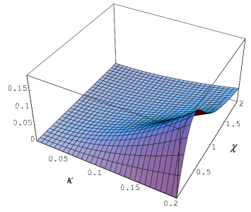
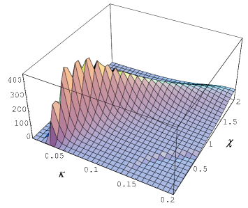
Figure 4: The dependence of the quantity $(T\sqrt{\varepsilon_{1}}\hbar c/q^{2})dN_{m}/d\vartheta d\phi$ on the undulator parameter $\kappa$ and the reduced angle $\chi$ for $\varepsilon_{0}=\varepsilon_{1}$ (left panel) and $\varepsilon_{0}=3\varepsilon_{1}$ (right panel). The values of the other parameters are $\gamma_{1\parallel}=10$, $m=1$, $\rho_{1}/\rho_{0}=1.05$.

6 Conclusion

Synchrotron radiation has become one of the most valuable and useful scientific tools with ever increasing applications for basic and applied research. In the present paper we have considered the influence of a dielectric cylinder on the synchrotron radiation from a charged particle moving along a helical orbit inside a dielectric cylinder. By using the Green function, we have derived formulae for the electromagnetic potentials and fields, Eqs. (14), (16), (18), and for the angular-frequency distribution of the radiation intensity emitted into the exterior medium. The latter is a sum of two terms. The first one, given by formula (27), is present when the Cherenkov condition for dielectric permittivity of the exterior medium and drift velocity of the charge is satisfied, $\beta_{1\parallel}>1$, and describes the radiation with a continuous spectrum propagating under the Cherenkov angle of the external medium. The second term in the total radiation intensity is given by formula (36), where the separate terms (37) describe the radiation, which for a given propagation direction has a discrete spectrum determined by formula (34). We have investigated various limiting cases of the general formula for the radiation intensity and have compared this formula to previously known special cases (radiation in vacuum, purely transversal synchrotron radiation, radiation from a charge moving with constant velocity along the axis parallel to the cylinder axis). In Section 4 we have investigated characteristic features of the radiation. Our numerical calculations have shown that under certain conditions strong narrow peaks appear in the angular distribution of the radiation intensity. By using asymptotic formulae for the cylindrical functions, we analytically argued the possibility for the presence of such peaks and the corresponding necessary conditions are specified. In particular, the peaks are present only when dielectric permittivity of the cylinder is greater than the permittivity for the surrounding medium and the Cherenkov condition is satisfied for the velocity of charge image on the cylinder surface and the dielectric permittivity of the cylinder. We have also estimated the width of these peaks. The peaks correspond to the opening angles for which the real part of the function $\alpha_{m}$ from (10) vanishes. The corresponding condition is in form (50) and is obtained from the equation determining the eigenmodes for the dielectric cylinder replacing the Hankel functions by the Neumann ones. In section 5 an application of the general formula is considered to the practically important case of the non-relativistic transverse motion when the longitudinal motion is relativistic. This type of motion can be produced by a variety of electromagnetic field structures and is used in helical undulators for generating electromagnetic radiation in a narrow spectral interval. Different regimes for the undulator parameter are considered corresponding to strong and weak undulators. In the former case the radiation intensity contains many harmonics and has sharp peaks at the opening angles determined by the zeros of the Bessel functions $J_{m}(\lambda_{0}\rho_{1})$. At the angles away from these peaks the radiation intensity is relatively suppressed by the factor $\gamma_{1\parallel}$. In the weak undulator regime the radiation is dominated by the fundamental harmonic and the leading contribution into the intensity comes from second term on the right of Eq. (15). In the case of a particle moving in a homogeneous medium this term vanishes and it is necessary to take the subleading terms. The corresponding numerical results are plotted in Figures 3 and 4. These results show that the presence of the cylinder provides a possibility for an essential enhancement of the radiated power as compared to the radiation in a homogeneous medium.

References

• [1] Handbook on Sinchrotron Radiation, edited by E.-E. Koch (North-Holland Publishing Company, Amsterdam, 1983).
• [2] Synchrotron Radiation Research, edited by H. Winick and S. Doniach (Plenum Press, New York, London, 1980).
• [3] A.A. Sokolov and I.M. Ternov, Radiation from Relativistic Electrons (ATP, New York, 1986).
• [4] I.M. Ternov, V.V. Mikhailin, and V.R. Khalilov, Synchrotron Radiation and its Applications (Harwood Academic Publishers, Amsterdam, 1985).
• [5] Synchrotron Radiation Theory and Its Development, edited by V.A. Bordovitsyn (World Scientific, Singapore, 1999).
• [6] A. Hofman, The Physics of Sinchrotron Radiation (Cambridge University Press, Cambridge, 2004).
• [7] G. B. Rybicky and A. P. Lightman, Radiative Processes in Astrophysics (J. Wiley, New York, 1979).
• [8] P. Rullhusen, X. Artru, and P. Dhez, Novel Radtiation Sources Using Relativistic Electrons (World Scientific, Singapore, 1998).
• [9] V.N. Tsytovich, Westnik MGU 11, 27 (1951, in Russian).
• [10] K. Kitao, Progr. Theor. Phys. 23, 759 (1960).
• [11] V.P. Zrelov, Wavilov–Cherenkov Radiation and Its Applications in High-Energy Physics (Atomizdat, Moscow, 1968, in Russian).
• [12] L.Sh. Grigoryan, A.S. Kotanjyan, and A.A. Saharian, Izv. Akad. Nauk Arm. SSR Fiz. 30, 239 (1995) [Sov. J. Contemp. Phys. 30, 1 (1995)].
• [13] S.R. Arzumanian, L.Sh. Grigoryan, Kh.V. Kotanjyan, and A.A. Saharian, Izv. Akad. Nauk Arm. SSR Fiz. 30, 106 (1995) [Sov. J. Contemp. Phys. 30, 12 (1995)].
• [14] L.Sh. Grigoryan, H.F. Khachatryan , and S.R. Arzumanyan, Izv. Akad. Nauk Arm. SSR Fiz. 33, 267 (1998) [Sov. J. Contemp. Phys. 33, 1 (1998)], cond-mat/0001322.
• [15] A.S. Kotanjyan, H.F. Khachatryan , A.V. Petrosyan, and A.A. Saharian, Izv. Akad. Nauk Arm. SSR Fiz. 35, (2000) [Sov. J. Contemp. Phys. 35, 1 (2000)].
• [16] A.S. Kotanjyan and A.A. Saharian, Izv. Akad. Nauk Arm. SSR Fiz. 36, (2001) [Sov. J. Contemp. Phys. 36, 7 (2001)].
• [17] A.S. Kotanjyan and A.A. Saharian, Mod. Phys. Lett. 17, 1323 (2002).
• [18] A.S. Kotanjyan, Nucl. Instrum. Methods B201, 3 (2003).
• [19] A.A. Saharian and A.S. Kotanjyan, Izv. Akad. Nauk Arm. SSR Fiz. 38, 288 (2003).
• [20] A.A. Saharian and A.S. Kotanjyan, Nucl. Instrum. Methods B, in press; hep-th/0403297.
• [21] A.A. Sokolov and I.M. Ternov, Zs. Phys. 211, 1 (1968).
• [22] D.F. Alferov, Yu.A. Bashmakov, and E.G. Bessonov, Sov. Phys. Tech. Phys. 18, 1335 (1974).
• [23] B.M. Kincaid, J. Appl. Phys. 48, 2684 (1977).
• [24] P. Luchini and H. Motz, Undulators and Free-electron Lasers (Clarendon, 1990).
• [25] M.M. Nikitin and V.Ya. Epp, Undulator Radiation (Energoatomizdat, Moscow, 1988, in Russian).
• [26] B.M. Bolotovsky, Usp. Fiz. Nauk 75, 295 (1961).
• [27] Handbook of Mathematical Functions, edited by M. Abramowitz and I.A. Stegun (Dover, New York, 1972).