A universal conformal field theory approach to the chiral persistent currents in the mesoscopic
fractional quantum Hall states

Abstract

We propose a general and compact scheme for the computation of the periods and amplitudes of the chiral persistent currents, magnetizations and magnetic susceptibilities in mesoscopic fractional quantum Hall disk samples threaded by Aharonov–Bohm magnetic field. This universal approach uses the effective conformal field theory for the edge states in the quantum Hall effect to derive explicit formulas for the corresponding partition functions in presence of flux. We point out the crucial role of a special invariance condition for the partition function, following from the Bloch–Byers–Yang theorem, which represents the Laughlin spectral flow. As an example we apply this procedure to the ${\mathbb{Z}}_{k}$ parafermion Hall states and show that they have universal non-Fermi liquid behavior without anomalous oscillations. For the analysis of the high-temperature asymptotics of the persistent currents in the parafermion states we derive the modular $S$-matrices constructed from the $S$ matrices for the $u(1)$ sector and that for the neutral parafermion sector which is realized as a diagonal affine coset.

1 Introduction

Mesoscopic physics has recently become a very intensive area of research because of the exciting opportunities it offers to observe fundamental implications of quantum mechanics in experimentally realizable two-dimensional samples. One important characteristics of the mesoscopic phenomena is that the electrons are coherent which implies that the sizes should be extremely small, the samples extremely pure and with high mobility and the temperatures very low.

According to a famous Bloch theorem the free energy of a conducting ring threaded by magnetic field is a periodic function of the magnetic flux through the ring with period one flux quantum $\phi_{0}=h/e=1$. The flux dependence of the free energy

$$F(T,\phi)=-k_{B}T\ln(Z(T,\phi)),$$ (1)

where $Z(T,\phi)$ is the partition function gives rise to an equilibrium current

$$I(T,\phi)=-\left(\frac{e}{h}\right)\frac{\partial F(T,\phi)}{\partial\phi},$$ (2)

called a persistent current, flowing along the ring without dissipation. These oscillating currents have universal amplitudes and temperature dependences and have been observed in mesoscopic rings [1], where the length of the ring is smaller than the coherence length at very low temperatures.

The fractional quantum Hall (FQH) states could be generically interpreted as mesoscopic rings because the only delocalized states live on the edge of the two-dimensional disk sample. The universality classes of the FQH systems have been successfully described by the effective field theories for the edge states in the thermodynamic scaling limit [2]. These turned out to be topological field theories in $2+1$ dimensional space-time which are equivalent to conformal field theories (CFT) on the $1+1$ dimensional space border, provided the bulk excitations are suppressed by a nonzero energy gap.

Most of the computations of the persistent currents in strongly correlated mesoscopic systems, including in the FQH regime, so far have been based mainly on the Fermi or Luttinger liquid picture [3, 4] because a more general approach to these quantities was missing. In this paper we shall formulate a general and compact scheme for the computation of the chiral persistent currents in mesoscopic FQH disk states based on the rational CFT on the edge. This scheme has become very important after recent experiments [5] showed that the (multicomponent) Luttinger liquid theory is irrelevant for more general filling factors such as those in the principle Jain series. We stress that the rational CFT description which is the right strategy for classifying the FQH universality classes is also the right starting point for the computation of the persistent currents in the FQH states. The main advantage of this approach is that the CFT partition function which is used as a thermodynamical potential can be computed analytically even when Aharonov–Bohm (AB) magnetic field is threading the sample. This fact has already been used in Refs. [6] and [7] for the computation of the persistent currents, magnetizations and the corresponding magnetic susceptibilities with the intuitive explanation that because the transformation $\zeta\to\zeta+\tau$ represents the addition of one flux quantum its generalization $\zeta\to\zeta+\phi\tau$ should be interpreted as adding flux $\phi$ in units $\phi_{0}=1$. We derive this result in Sect. 2.8 which was one of the motivations for the present paper. The fact that the magnetic field is of AB type (i.e., an infinitely long and thin solenoid) is a significant simplification because the AB magnetic field is zero at the edge so that it does not break the conformal invariance. On the other hand this limitation is not completely restrictive because the edge of a FQH system is so thin that the free energy depends only on the flux encircled by the edge and not on the magnetic field alone. Adding AB flux to the FQH system naturally introduces twisted boundary conditions for the field operators of the electron and quasiparticles and also modifies the effective Hamiltonian. We show that the ultimate effect of this twisting on the partition function is that it is multiplied by a universal exponential factor and that the modular parameter $\zeta$ is shifted by an amount proportional to the modular parameter $\tau$ where the coefficient of proportionality coincides with the AB flux $\phi$. As an illustration of the general CFT approach to the chiral persistent currents we are computing these currents for the parafermion FQH states using the partition functions developed in [8].

The persistent currents in the FQH regime typically contain large non-mesoscopic components [9], slowly varying with the magnetic field, which cannot be described within the CFT framework since there are contributions from states laying deep below the Fermi level. The edge states effective CFT is relevant only for the computation of the much smaller oscillating part of the persistent currents which could nevertheless be tested directly in SQUID detectors [1] using the Josephson effect. While the persistent currents naturally express the electric properties of the system, it turns out that they could also give important information about the neutral structure of the effective field theory for the edge states [3, 10]. As we shall demonstrate in Sect. 4.3 and Sect. 4.4 the low- and high- temperature decays of the persistent current’s amplitudes crucially depend on the neutral properties of the edge states. Our analysis reveals two different universal mechanisms for the thermal reduction of the persistent currents: at low temperatures the thermal activation of quasiparticle–quasihole pairs leads to a logarithmic decay of the amplitudes while at high temperatures the reduction is due to thermal decoherence and the decay is exponential.

The rest of this paper is organized as follows: in Sect. 2 we review the rational CFT approach to the FQH states, describe in brief the terminology of the chiral quantum Hall lattices of topological charges which is necessary for the understanding of the general classification of FQH universality classes. In Sect. 2.8 we show how the CFT partition function is modified by the AB flux starting from the twisting of the electron field and deriving explicitly the modification of the ${\widehat{u(1)}}$ current and the Hamiltonian. In Sect. 2.9 we discuss the Laughlin spectral flow, the role of the Cappelli–Zemba factors for restoring the invariance of the partition function under this flow and prove that the CFT partition function with AB flux is invariant under $\phi\to\phi+1$ as it should be according to the Bloch–Byers–Yang theorem. In Sect. 2.10 we derive the low-temperature asymptotics of the CFT partition function, which is universal. This asymptotics is then used in Sect. 4.3 to derive the low-temperature asymptotics of the persistent currents amplitudes which have a universal form and is expected to be valid for all FQH states. In Sect. 2.11 we show how to use the modular $S$ transformation in a rational CFT to analyze the high-temperature asymptotics of the partition functions and the persistent currents. In Sect. 3 we summarize the results from Ref. [8] about the partition functions for the edge states of the parafermion (PF) FQH states for $k=2,3$ and $4$. We derive analytically in Sect. 3.2 the complete $S$ matrix for the parafermion states as well as that for the neutral part which is realized as a diagonal affine coset. Then we investigate the persistent currents for fixed temperature when the flux is varied within one period as well as the temperature decay of the amplitude. In Sect. 4.4 the high-temperature asymptotics for the parafermion FQH states is computed using the analytic $S$ matrices derived in Sect. 3.2. Some technical details are put in several appendices.

2 Chiral partition function for the FQH states with Aharonov–Bohm flux

2.1 CFT for the edge states: labeling the FQH universality classes

Due to the existence of a nonzero energy gap in the FQH effect excitations spectrum the electron system behaves as an incompressible electron liquid at low energies. The effective field theory in the scaling thermodynamic limit, which essentially describes the low-energy excitations, turns out to be a topological relativistic quantum field theory in 2+1 dimensions with a Chern–Simons action. It is well known that these theories are equivalent to CFTs on the 1+1 dimensional edge. Therefore, it is believed that the CFT could capture all universal properties of the FQH systems and thus allow us to make a complete classification of the QH universality classes.

The electric current on the edge, where the coordinates are denoted by $\{x_{\alpha}\}$ for $\alpha=1,2$ and $\{A_{\alpha}\}$ is the restriction of the vector potential to the edge, is anomalous [11]

$$\partial_{\alpha}j^{\alpha}=\frac{1}{2}\sigma_{H}\epsilon_{\alpha\beta}F_{\alpha\beta},\quad\sigma_{H}=\frac{e^{2}}{h}\nu_{H},\quad F_{\alpha\beta}=\partial_{\alpha}A_{\beta}-\partial_{\beta}A_{\alpha},$$

i.e., it violates the $u(1)$ invariance on the edge, however, this is exactly compensated by the violation of the $u(1)$ invariance in the bulk so that the sum of the bulk and edge current is invariant. This compensation of bulk and edge anomalies is the origin of the so called holographic principle [11] which in this case can be formulated as the correspondence between the quasiparticle spectra on the edge and in the bulk. The $u(1)$ anomaly mentioned above is the basic mechanism through which the Hall current is transmitted between the two edges of the real FQH samples.

2.2 The $\widehat{u(1)}\times Vir$ symmetry

The chiral CFT describing the edge of a FQH system always contains a separate $\widehat{u(1)}$ and Virasoro ($Vir$) symmetries. The first one describes the electric charge $Q$, or equivalently the magnetic flux $\phi$ properties due to the fundamental FQH relation [2]

$$Q=\nu_{H}\,\phi,$$ (3)

($e=1$) while the second corresponds to the angular momentum. Note that due to the Sugawara formula the ${\widehat{u(1)}}$ sector contributes to the angular momentum as well so by $Vir$ in the relative $\widehat{u(1)}\times Vir$ decomposition we mean the Virasoro contribution from the neutral sector only. As we shall see in Sect. 2.4 the neutral $Vir$ sector must be present for all FQH states with filling factors whose numerators are bigger than $1$.

The chiral partition function $Z(\tau,\zeta)$ corresponding to a disk FQH sample with a single edge computed within the effective CFT for the edge states

$${Z}(\tau,\zeta)=\mathop{\mathrm{tr}}_{\ \ {\mathcal{H}}\ }q^{L_{0}-c/24}\,\exp\left(2\pi i\zeta J_{0}^{\mathrm{el}}\right)=\sum_{\lambda=1}^{\mathcal{N}}\chi_{\lambda}(\tau,\zeta),$$ (4)

is the linear sum of all topologically distinct chiral CFT characters [7]

$$\chi_{\lambda}(\tau,\zeta)=\mathop{\mathrm{tr}}_{\ \ {\mathcal{H}}_{\lambda}\ }q^{L_{0}-c/24}\,\exp\left(2\pi i\zeta J_{0}^{\mathrm{el}}\right)\ \ \mathrm{where}\ \ {\mathcal{H}}=\mathop{\oplus}_{\lambda=1}^{\mathcal{N}}{\mathcal{H}}_{\lambda}.$$ (5)

The number $\mathcal{N}$ in Eqs. (4), called the topological order [12], (the number of topologically inequivalent quasiparticles with electric charge [11] $0\leq Q_{\mathrm{el}}<1$) is one of the most important characteristics of the FQH universality classes. The Hilbert space of the edge states ${\mathcal{H}}$, over which the traces in Eqs. (4) and (5) are taken, is the direct sum of all independent (i.e., irreducible, topologically inequivalent) representations ${\mathcal{H}}_{\lambda}$ of the chiral algebra which are closed under fusion (see the Introduction of Ref. [13] for a short description of the chiral algebra terminology in the FQH effect context). The effective Hamiltonian for the edge states in the thermodynamic limit is given by [14]

$$H_{\mathrm{CFT}}=\frac{v_{F}}{R}\left(L_{0}-\frac{c}{24}\right),\quad L_{0}=\oint\frac{d\,z}{2\pi i}\ z\,T(z),\quad z=\exp\left(\frac{v_{F}\,t-i\,x}{R}\right),$$ (6)

where $x$ is the coordinate on the edge, $t$ is the imaginary time, $v_{F}$ is the Fermi velocity on the edge, $R$ is its radius, $L_{0}$ is the zero mode of the Virasoro stress tensor $T(z)$ and $c$ is the central charge of the latter [15]. The CFT Hamiltonian (6) captures the universal properties of realistic FQH systems and could eventually give a qualitative description of the Hilbert space structure of the low-lying excitations [16], the energy spectrum and even the (universal part of the) energy gap [13] of the FQH systems in the thermodynamic limit. In particular, it should not be surprising that the CFT-based computations [10] of the persistent currents in the Laughlin FQH states give the same results as those based on the Luttinger liquid picture [4].

The electric charge operator $J^{\mathrm{el}}_{0}$ in Eq. (4), defined as the space integral of the charge density $J^{\mathrm{el}}(z)$ on the edge, which is proportional to the normalized $\widehat{u(1)}$ current

$$J(z)=i\,\partial\phi^{(c)}(z)=\sum_{n\in{\mathbb{Z}}}J_{n}\,z^{-n-1},\quad\left[J_{n},J_{m}\right]=n\,\delta_{n+m,0},$$ (7)

has the following short-distance operator product expansion [2, 15, 14, 13]

$$J_{0}^{\mathrm{el}}=\oint\frac{d\,z}{2\pi i}\,J^{\mathrm{el}}(z),\quad J^{\mathrm{el}}(z)=\sqrt{\nu_{H}}\,J(z),\quad J^{\mathrm{el}}(z)J^{\mathrm{el}}(w)\sim\frac{\nu_{H}}{(z-w)^{2}}.$$ (8)

The modular parameters $q$ and $\zeta$ entering Eq. (5) are generically restricted in annulus samples for convergence by

$$q=\mathrm{e}^{2\pi i\tau},\quad\mathrm{Im}\,\tau>0,\quad\left(\mathrm{Im}\,\tau\sim 1/k_{B}T\right)\quad\zeta\in{\mathbb{C}}$$

and their real and imaginary parts are related to the inverse temperature, chemical potential and Hall voltage [14]. For the disk FQH sample, however, both $\tau$ and $\zeta$ have to be purely imaginary in order for the partition function Eq. (4) be real. The physical meaning of $\mathrm{Im}\,\tau$ and $\mathrm{Im}\,\zeta$ will be discussed in Sect. 2.9.

Because the AB flux modifies only the charged ${\widehat{u(1)}}$ sector of the model it would be convenient to artificially split the stress tensor into a charged and a neutral parts

$$T(z)=T^{(c)}(z)+T^{(0)}(z),\quad\mathrm{where}\quad T^{(c)}(z)=\frac{1}{2}\,{\mbox{{:}}{J(z)^{2}}{\textrm{:}}}$$ (9)

is the Sugawara stress tensor of ${\widehat{u(1)}}$ and $T^{(0)}=T-T^{(c)}$ is its complement.

2.3 Abelian rational CFTs: FQH states classification in terms of integer lattices of topological charges

The CFTs which naturally appear [2] in the FQH effect context are rational extension of the ${\widehat{u(1)}}^{N}$ current algebra in terms of integer lattices of topological charges. A central result in this approach is the complete A-D-E classification of the FQH universality classes in terms of abelian rational CFT associated with those lattices [2]. We recall that an abelian theory is a rational conformal field theory with integer central charge $c=N$ and ${\widehat{u(1)}}^{N}$ affine symmetry; the current algebra is generated by $N$ abelian currents $J^{a}(z)=i\partial_{z}\phi^{a}(z)$, extended by the vertex operators $Y(\lambda,z)={\mbox{{:}}{\exp(i\lambda_{a}\phi^{a}(z))}{\textrm{:}}}$, whose “topological charges” $\lambda_{a}$ form a $N$-dimensional lattice $\Gamma$. The lattices which appear in the quantum Hall effect must satisfy some specific physical conditions which are summarized bellow. Following Ref.[2], we call chiral quantum Hall lattice an odd integral lattice to which a special charge vector $\underline{Q}$ from the dual lattice $\Gamma^{*}$ is associated. This vector assigns to any lattice point $\underline{q}\in\Gamma$ the electric charge $(\underline{q}|\underline{Q})$ of the corresponding edge excitation. In particular, the lattice should contain an electron excitation $\underline{q}_{\mathrm{el}}$ with unit charge $(\underline{q}_{\mathrm{el}}|\underline{Q})=-1$. The norm $|\underline{q}|^{2}=(\underline{q}|\underline{q})$ of the vectors $\underline{q}\in\Gamma$ gives twice the conformal dimensions, i.e. twice the spin of the corresponding excitation, while the scalar product $(\underline{q}|\underline{q}^{\prime})$ is the relative statistics of the excitations $\underline{q}$ and $\underline{q}^{\prime}$.

The charge vector $\underline{Q}$ satisfies the following conditions:

  (i)

it is primitive, i.e., not a multiple of any other vector $\underline{q}^{*}\in\Gamma^{*}$;

(ii)

it is related to $\nu_{H}$ by:

$$|\underline{Q}|^{2}=\nu_{H}=\frac{n_{H}}{d_{H}},\quad n_{H},d_{H}\in{\mathbb{N}},\quad\mathrm{gcd}(n_{H},d_{H})=1;$$ (10)

(iii)

it obeys the charge–statistics relation for boson/fermion excitations:

$$(\underline{Q}|\underline{q})=|\underline{q}|^{2}\quad\ \mathrm{mod}\ \ 2\ ,\qquad{\rm for\ any}\ \underline{q}\in\Gamma.$$ (11)

We shall briefly recall the notion of maximal symmetry [2] since it covers the largest class of QH lattices. A chiral Hall lattice is called maximally symmetric if its neutral sublattice ($\Gamma_{0}\perp\underline{Q}$) coincides with the (internal symmetry) Witt sublattice $\Gamma_{W}\subset\Gamma$ (defined as the sublattice generated by all vectors of square length 1 or 2) so that dim $\Gamma_{W}=$ dim $\Gamma-1$. The Witt sublattice is always of the type $A\oplus D\oplus E\oplus{\mathbb{Z}}$. The maximally symmetric lattices, denoted in [2] by the symbol $(L|\,{}^{\underline{\omega}}\Gamma_{W})$, can be characterized in an appropriate basis $\{\underline{q}^{i}\}$ by the following Gram matrix $G=(G^{ij})$ where $G^{ij}=(\underline{q}^{i}|\underline{q}^{j})$ is the metrics of the lattice:

$$G=\left[\begin{array}[]{c|c}L&\underline{\omega}\cr\hline\cr\underline{\omega}^{T}&C(\Gamma_{W})\end{array}\right],\quad\det(G)=\frac{1}{\nu_{H}}\det\left[C(\Gamma_{W})\right];$$ (12)

the charge vector is $Q=(1,0,\ldots,0)$ in the corresponding dual basis. Here $L\in{\mathbb{N}}$ is the minimal relative angular momentum that appears as the minimal power of $(z_{i}-z_{j})$ in the corresponding wave function; $C(\Gamma_{W})$ is the Cartan matrix for the Witt sublattice and $\underline{\omega}$ is an admissible weight for $\Gamma_{W}$ restricted by the condition $(\underline{\omega}|\underline{\omega})<L$ (see Eq. (5.6) in [2]). Note that the Witt sublattice does not contribute to the filling fraction $\nu_{H}$ since it is orthogonal to the charge vector $\underline{Q}$. It is easy to find $\nu_{H}$ corresponding to the lattice with the Gram matrix (12) using Eq. (10),

$$\nu_{H}=(\underline{Q}|\underline{Q})=Q^{T}.G_{\Gamma}^{-1}.Q=\frac{1}{L-(\underline{\omega}|\underline{\omega})}\ .$$ (13)

The non-equivalent quasi-particles in the Hall state correspond to the irreducible representations of the extended algebra and are labelled by the points $\underline{\lambda}\in\Gamma^{*}/\Gamma$ where $\underline{\lambda}$ is the quasiparticle’s topological charge and $\Gamma^{*}$ is the lattice dual to $\Gamma$. We recall that $\Gamma^{*}/\Gamma$ is a finite abelian group of order $(\det\Gamma)$ whose multiplication law represents the fusion rules. There are several important consequences of the specific structure of the Gram matrix (12) and FQH effect specifics which we consider in more detail in the next subsections.

2.4 The electron charge decomposition

The Gram matrix (12) implies that the topological charge $\underline{q}_{\mathrm{el}}$ of the electron should take the form [2]

$$\underline{q}_{\mathrm{el}}=-\frac{1}{\nu_{H}}\ \underline{Q}+\underline{\omega},$$ (14)

where $\underline{Q}$ is the lattice charge vector and $\underline{\omega}$, which is the weight entering Eq. (12) i.e., an admissible weight of the Witt sublattice [2], represents the neutral degrees of freedom of the electron because $(\underline{Q}|\underline{\omega})=0$. Then the electron field operator would be simply a tensor product of a ${\widehat{u(1)}}$ vertex exponent of a chiral boson $\phi$, which is a simple current of the ${\widehat{u(1)}}$ theory, and in general a simple current $\Phi_{\underline{\omega}}$ from the neutral part of the theory

$$\psi_{\mathrm{el}}(z)={\mbox{{:}}{\exp\left(-i\frac{1}{\sqrt{\nu_{H}}}\phi^{(c)}(z)\right)}{\textrm{:}}}\otimes\ \Phi_{\underline{\omega}}(z),$$ (15)

where $\phi^{(c)}(z)$ is the normalized chiral ${\widehat{u(1)}}$ boson corresponding to the charged component of the electron and $\Phi_{\underline{\omega}}(z)$ is a primary field ($\underline{\omega}$ is a simple current, i.e., $\underline{\omega}*\bar{\underline{\omega}}=1$ [15, 17]) from the neutral sector with CFT dimension $(\underline{\omega}|\underline{\omega})/2$

$$\phi^{(c)}(z)\phi^{(c)}(w)\sim-\ln(z-w),\quad\Phi_{\underline{\omega}}(z)\Phi_{\underline{\omega}}^{*}(w)\sim\frac{1}{(z-w)^{(\underline{\omega}|\underline{\omega})}}.$$

Next, due to the charge–statistics relation (11), the conformal dimension of the electron which is

$$\Delta_{\mathrm{el}}=\frac{1}{2}(\underline{q}_{\mathrm{el}}|\underline{q}_{\mathrm{el}})=\frac{1}{2}\left(\frac{1}{\nu_{H}}+(\underline{\omega}|\underline{\omega})\right)=\frac{1}{2\nu_{H}}+\Delta^{(0)}(\underline{\omega}),\quad\Delta^{(0)}(\underline{\omega})=(\underline{\omega}|\underline{\omega})\geq 0\quad$$ (16)

must be equal to $p+1/2$ for some $p\in{\mathbb{Z}}_{+}$. According to Eqs. (14) and (16) the neutral component $\underline{\omega}$ of the electron should certainly give a nontrivial fractional contribution to the CFT dimension when the numerator of the filling factor $\nu_{H}$ is bigger than $1$. Therefore, in general, the neutral component $\Phi_{\underline{\omega}}(z)$ of the electron field operator cannot be completely removed without violating the fermionic statistics of the electron. Note that the condition $(\underline{\omega}|\underline{\omega})\geq 0$ in Eq. (16) is equivalent to $l_{\mathrm{max}}\geq 1/\nu_{H}$ as formulated in Ref. [2].

2.5 Spin–charge separation and ${\mathbb{Z}}_{n_{H}}$ Pairing rule

Because the weight $\underline{\omega}\neq 0$ has at least one non-zero component when the numerator of the filling factor is $n_{H}>1$ the Gram matrix (12) in this case is not decomposable, i.e, it cannot be represented as a direct sum of two matrices with smaller dimensions. This implies that the dual lattice would not be decomposable either so that the inequivalent irreducible representations of the chiral algebra, i.e., the quasiparticles, would not be simple tensor products of charged and neutral vertex exponents but actually sums of such. Therefore the charge and spin are entangled and this absence of spin–charge separation makes the situation more complicated. Nevertheless, the spin–charge decomposition could be achieved at the expenses of enlarging the dual lattice (of excitations) and of introducing a selection rule (the ${\mathbb{Z}}_{n_{H}}$ pairing rule). In fact, there exists a decomposable sublattice $L\subset\Gamma$ of the same dimension $N$ spanned by the vectors

$$\{\underline{\mathrm{e}}^{1},\underline{\alpha}_{i}\}\ ,\qquad\underline{\mathrm{e}}^{1}=n_{H}(\underline{q}_{\mathrm{el}}-\underline{\omega})=\underline{Q}\,d_{H},$$ (17)

where $\left\{\underline{\alpha}_{i}\right\}$ are the basis vectors of the neutral sublattice $\Gamma_{W}\subset\Gamma$, i.e., the simple roots of the Cartan lattice. This sublattice indeed splits into 2 mutually orthogonal sublattices:

$$L={\mathbb{Z}}\underline{Q}\ d_{H}\oplus\Gamma_{W}\ .$$ (18)

We have the inclusions $L\subset\Gamma\subset\Gamma^{*}\subset L^{*}$ and the physical lattice $\Gamma$ can be decomposed in terms of its sublattice $L$ as follows

$$\Gamma=\left\{\underline{\gamma}=\underline{\lambda}+s\ \underline{q}_{\mathrm{el}}\;\Big{|}\;\underline{\lambda}\in L,\;0\leq s\leq n_{H}-1\right\},$$ (19)

i.e., $\forall\underline{\gamma}\in\Gamma$, $\exists!\,\underline{\lambda}\in L,$ and $\exists!\,s\in{\mathbb{Z}}_{n_{H}}$ such that $\underline{\gamma}=\underline{\lambda}+s\underline{q}_{\mathrm{el}}$. Note that $L^{*}/\Gamma^{*}\simeq\Gamma/L\simeq{\mathbb{Z}}_{n_{H}}$ since the determinants of the Gram matrices of $L$ and $\Gamma$ (which give the number of sectors of the corresponding rational conformal theory) are:

$$|L|=d_{H}^{2}|\underline{Q}|^{2}|C_{W}|^{2}=n_{H}\,d_{H}\;\det(C_{W})=n_{H}^{2}|\Gamma|.$$ (20)

The spin–charge separation of excitations is achieved in the decomposable dual lattice $L^{*}$, whose physical points (corresponding to the points of $\Gamma^{*}$) obey a “$\ \mathrm{mod}\ \ n_{H}$”-selection rule: if $\underline{\lambda}\in L^{*}/L$ then $\underline{\lambda}$ is a physical excitation (i.e., $\underline{\lambda}\in\Gamma^{*}/\Gamma$) iff

$$\forall\underline{\lambda}\in L^{*}/L:\quad\underline{\lambda}\in\Gamma^{*}/\Gamma\subset L^{*}/L\quad\Longleftrightarrow\quad\left(\underline{q}_{\mathrm{el}}|\underline{\lambda}\right)\in{\mathbb{Z}}.$$

In other words, if we write the excitation charge $\underline{\lambda}$ in the basis of $L^{*}$

$$\underline{\lambda}=l\,\underline{\mathrm{e}}^{*}_{1}+\underline{\Lambda},\quad\underline{\Lambda}=\sum_{i}a^{i}\underline{\Lambda}_{i},\quad l,\,a^{i}\in{\mathbb{Z}}$$ (21)

with $\underline{\Lambda}_{i}$ being the fundamental weights of the Witt sublattice, then $\underline{\lambda}$ is a physical excitation if

$$\left(\underline{q}_{\mathrm{el}}|\underline{\lambda}\right)=\frac{1}{n_{H}}\left(n_{H}(\underline{\omega}|\underline{\Lambda})-l\right)\in{\mathbb{Z}}\quad\Longleftrightarrow\quad n_{H}(\underline{\omega}|\underline{\Lambda})=l\ \mathrm{mod}\ n_{H},$$ (22)

where $\underline{\omega}=\sum_{i}\omega^{i}\underline{\Lambda}_{i}$ with $\omega^{i}\in{\mathbb{Z}}$ is the neutral component of the electron’s topological charge (14). This condition reduces the number of elements in $L^{*}/L$ by a factor of $n_{H}^{2}$ to that of $\Gamma^{*}/\Gamma$ which is the number of physically different quasiparticles. To summarize, we first extend the dual lattice $\Gamma^{*}$ to $L^{*}$ obtaining the spin–charge separation in the latter and then identify the physical points in the extended lattice $L^{*}$ by a ${\mathbb{Z}}_{n_{H}}$ pairing rule.

2.6 The CFT characters for the lattice extensions of ${\widehat{u(1)}}^{N}$

Because of Eq. (19) the Hilbert spaces ${\mathcal{H}}^{\Gamma}$of the original $\Gamma^{*}/\Gamma$ model can be written as direct sums of the Hilbert spaces ${\mathcal{H}}^{L}$ of its decomposable sublattice (18)

$${\mathcal{H}}^{\Gamma}_{\underline{\gamma}^{*}}=\mathop{\oplus}\limits_{\underline{\gamma}\in\Gamma}\mathcal{V}_{\underline{\gamma}^{*}+\underline{\gamma}}=\mathop{\oplus}\limits_{s\ \mathrm{mod}\ n_{H}}\ \ \mathop{\oplus}\limits_{\underline{\lambda}\in L}\mathcal{V}_{\underline{\gamma}^{*}+\underline{\lambda}+s\underline{q}_{\mathrm{el}}}=\mathop{\oplus}\limits_{s\ \mathrm{mod}\ n_{H}}{\mathcal{H}}^{L}_{\underline{\gamma}^{*}+\underline{\lambda}+s\underline{q}_{\mathrm{el}}},$$

where $\mathcal{V}_{\underline{\gamma}^{*}}$ is the ${\widehat{u(1)}}^{N}$ Verma module ($N\in{\mathbb{N}}$ is the rank of the lattice $\Gamma$) over the lowest-weight state $|\underline{\gamma}^{*}\rangle$. Therefore the $\Gamma$-characters would have a similar decomposition into $L$-characters

$$\chi_{\underline{\gamma}^{*}}(\tau,\zeta;\Gamma)=\mathop{\mathrm{tr}}_{\ \ {\mathcal{H}}_{\underline{\gamma}^{*}+s\underline{q}_{\mathrm{el}}}^{L}\ }q^{L_{0}-c/24}\,\mathrm{e}^{2\pi i\zeta(\underline{Q}|\underline{J}_{0})}\ =\sum_{s\ \mathrm{mod}\ n_{H}}\chi_{\underline{\gamma}^{*}+s\underline{q}_{\mathrm{el}}}(\tau,n_{H}\zeta;L),$$

where the factor $n_{H}$ in front of $\zeta$ appeared because $\underline{Q}=\underline{q}^{*}_{1}$ in $\Gamma^{*}$ but in the decomposable dual lattice it is $\underline{Q}=n_{H}\,\underline{\mathrm{e}}^{*}_{1}\in L^{*}$. Because the sublattice $L$ is decomposable the characters of the ${\mathcal{H}}^{L}$ modules are simply products of those for the corresponding charged and neutral sectors. Writing explicitly $\underline{\gamma}^{*}=l\,\underline{\mathrm{e}}^{*}_{1}+\underline{\Lambda}$ we have

$$\chi_{l,\underline{\Lambda}}(\tau,\zeta;\Gamma)=\sum_{s\ \mathrm{mod}\ n_{H}}K_{l+sd_{H}}(\tau,n_{H}\zeta;n_{H}d_{H})\ \mathrm{ch}_{\underline{\omega}^{s}*\underline{\Lambda}}(\tau)$$ (23)

where $K_{l}(\tau,n_{H}\zeta;n_{H}d_{H})$ is the character of the (charged) ${\widehat{u(1)}}$ sector, i.e., the rational torus partition function [15]

$$K_{l}(\tau,\zeta;m)=\frac{1}{\eta(\tau)}\sum_{n\in{\mathbb{Z}}}q^{\frac{m}{2}\left(n+\frac{l}{m}\right)^{2}}\mathrm{e}^{2\pi i\zeta\left(n+\frac{l}{m}\right)},\quad\eta(\tau)=q^{\frac{1}{24}}\prod_{n=1}^{\infty}\left(1-q^{n}\right),$$ (24)

($\eta$ is the Dedekind function [15]) while $\mathrm{ch}_{\underline{\Lambda}}(\tau)$ is that of the neutral sector of the decomposable lattice $L$ and $\underline{\Lambda}$ satisfies the ${\mathbb{Z}}_{n_{H}}$ pairing rule $n_{H}(\underline{\omega}|\underline{\Lambda})=l\ \mathrm{mod}\ n_{H}$. Note that the electron charge vector (14) acts on the neutral sector by the $s$-th power of the simple current $\underline{\omega}$ which in an abelian CFT is taking the form $\underline{\omega}^{s}*\underline{\Lambda}=s\underline{\omega}+\underline{\Lambda}$. The characters expressions (23) are valid for the FQH state corresponding to the arbitrary topological charge lattice $\Gamma$.

2.7 Neutral reductions and stability criteria

The classification of the FQH universality classes in terms of chiral quantum Hall lattices is motivated by the rationality of the filling factors and of the electric charge spectrum. In addition, according to Eq. (16) the neutral component $\underline{\omega}$ of the electron’s topological charge should also have a rational CFT dimension depending on the filling factor (see Eq. (13)). That is why the electric properties of the FQH liquid are well-described by the topological charge lattice extension of the ${\widehat{u(1)}}^{N}$ CFT introduced in Sect. 2.3. However the electric properties, which are basically what is measured in the experiment, are not enough to fix a unique rational CFT corresponding to a given FQH universality class. For example, we can start with the lattice extension of the ${\widehat{u(1)}}^{N}$ CFT and project some degrees of freedom in the neutral sector keeping the same electric ${\widehat{u(1)}}$ part. This would certainly preserve the electric properties and produce another candidate CFT for the same universality class. Two important consistency conditions are that the neutral projection preserves the neutral component $\underline{\omega}$ of the electron topological charge vector, for locality reasons, and the ${\mathbb{Z}}_{n_{H}}$ pairing rule which is a general property of the FQH excitations due to the spin–charge entanglement. The advantage of the neutral projections is that they generically reduce the total central charge and therefore may produce better candidates for the same universality class according to the stability criteria formulated in Ref. [11]. The neutral projections also preserve the structure of the characters (23) only the neutral characters $\mathrm{ch}_{\underline{\omega}^{s}*\underline{\Lambda}}$ have to be replaced by the corresponding projected ones. This is important because the neutral characters give non-trivial contribution to all thermodynamic quantities. An example of a neutral projection which we shall describe in Sect. 3 is the affine coset reductions which realizes the parafermion FQH states in the second Landau level [8].

The FQH effect phenomenology seems to be in favor of the neutral projections: the main quantum numbers expected in single-layer disk QH samples of polarized electrons are electric charge and orbital momentum, while in the lattice extensions of ${\widehat{u(1)}}^{N}$ there are $N$ separately conserved charges. The projection would remove the superfluous charges keeping only the electric charge and the orbital momentum, and in some cases would preserve discrete quantum numbers related to $W_{n}$ algebras, like in the coset projection in Sect. 3, due to the ${\mathbb{Z}}_{n_{H}}$ pairing rule.

2.8 The Aharonov–Bohm flux: twisting the electron

Let us introduce the AB magnetic field piercing the FQH disk sample at the origin in the $z$ direction which is produced by a vector potential of the form

$$\mathbf{A}=\frac{h}{e}\frac{\phi}{2\pi r^{2}}\,(-y,x)=\frac{h}{e}\frac{\phi}{2\pi r}\ \mathbf{e_{\varphi}},\quad\mathrm{where}\quad r=\sqrt{x^{2}+y^{2}}$$ (25)

is the length of the radius vector $\mathbf{r}=(x,y)$ in the plane, $\mathbf{e_{\varphi}}$ is the unit vector along the direction of the polar angle $\varphi$ and $\phi\in{\mathbb{R}}$ is the AB magnetic flux in units of the flux quantum $\phi_{0}=h/e$. In this section we shall see how the partition function is modified in presence of AB flux.

First, because $\mathrm{rot}\,\mathbf{A}=\phi\ \delta^{(2)}(\mathbf{r})$ is zero everywhere except for the origin, the electron field $\psi^{A}_{\mathrm{el}}(z)$ in presence of AB flux can be written as

$$\psi^{A}_{\mathrm{el}}(z)=\exp\left(-i\frac{e}{\hbar}\int_{*}^{z}\mathbf{A}.\d\mathbf{r}\right)\ \psi_{\mathrm{el}}(z)=z^{-\phi}\ \psi_{\mathrm{el}}(z),\quad\phi\in{\mathbb{R}},$$ (26)

($e=\hbar=1$) where $\psi_{\mathrm{el}}(z)$ is the electron field operator in the absence of AB magnetic field, provided that the path of the line integral does not encircle the origin. In the computation of the line integral in Eq. (26) we have used $z=r\exp(i\varphi)$ and have chosen a path along the $\varphi$ coordinate line , i.e., $\d\mathbf{r}=r\,\mathbf{e_{\varphi}}\d\varphi$, ending at $\varphi=\arg(z)$, the polar angle of the coordinate $z$. The second equality in Eq. (26) is a simple special case of a more general procedure called twisting [18, 19]. The AB flux modifies only the ${\widehat{u(1)}}$ part of the electron operator (15) which, for any QH system (integer and fractional), is realized as the ${\widehat{u(1)}}$ vertex exponent defined by

$${\mbox{{:}}{\mathrm{e}^{i\alpha\phi^{(c)}(z)}}{\textrm{:}}}\ \stackrel{{\scriptstyle\mathrm{def}}}{{=}}\ U_{\alpha}\,\mathrm{e}^{i\alpha\phi^{(c)}_{+}(z)}\,z^{\alpha J_{0}}\,\mathrm{e}^{i\alpha\phi^{(c)}_{-}(z)},\quad i\phi^{(c)}_{\pm}(z)=\pm\sum_{n=1}^{\infty}J_{\mp n}\frac{z^{\pm n}}{n},$$ (27)

where $U_{\alpha}$ are outer automorphisms of the ${\widehat{u(1)}}$ current algebra satisfying $U_{\alpha}\,U_{\beta}=U_{\alpha+\beta}$ for $\alpha,\beta\in{\mathbb{R}}$, $U_{0}=1$, $\left(U_{\alpha}\right)^{\dagger}=U_{-\alpha}$ and

$$\left[J_{n},U_{\alpha}\right]=\alpha\,U_{\alpha}\,\delta_{n,0}.$$ (28)

Therefore we can use the well known results [18] for the twisting of the normalized ${\widehat{u(1)}}$ current, ${\widehat{u(1)}}$ Sugawara stress tensor and normal ordered exponentials. The twisting with a twist $\beta$ is the transformation [18] $\pi_{\beta}\ :\ A\to U_{\beta}\,A\,U_{-\beta}$ for any operator $A$ from the chiral (observable) algebra; in particular twisting of the vertex exponents gives

$${\mbox{{:}}{\mathrm{e}^{i\alpha\phi^{(c)}(z)}}{\textrm{:}}}\quad\stackrel{{\scriptstyle\pi_{\beta}}}{{\longrightarrow}}\quad U_{\beta}\,{\mbox{{:}}{\mathrm{e}^{i\alpha\phi^{(c)}(z)}}{\textrm{:}}}\,U_{-\beta}=z^{-\alpha\beta}\,{\mbox{{:}}{\mathrm{e}^{i\alpha\phi^{(c)}(z)}}{\textrm{:}}}$$ (29)

which can be computed directly by using the definition  (27) and the commutation relations (28) and (7). Because the twisted electron operator

$$\pi_{\beta}\left(\psi_{\mathrm{el}}\right)(z)=\pi_{\beta}\left({\mbox{{:}}{\mathrm{e}^{-\frac{i}{\sqrt{\nu_{H}}}\phi^{(c)}(z)}}{\textrm{:}}}\right)\Phi_{\underline{\omega}}(z)=z^{\frac{1}{\sqrt{\nu_{H}}}\beta}\psi_{\mathrm{el}}(z)$$ (30)

has to reproduce Eq. (26) the value of the twist $\beta$ corresponding to the addition of AB flux $\phi$ can be determined by

$$-\left(\frac{-1}{\sqrt{\nu_{H}}}\right)\,\beta=-\phi\quad\Rightarrow\quad\beta=-\sqrt{\nu_{H}}\,\phi.$$

Then the normalized ${\widehat{u(1)}}$ current (7) is modified as follows [18]

$$J(z)\quad\stackrel{{\scriptstyle\pi_{\beta}}}{{\longrightarrow}}\quad U_{\beta}\,J(z)\,U_{-\beta}=J(z)-\frac{\beta}{z},$$ (31)

which again can be computed from the definition (7) of the current and the commutation relations (28). Next, the twist of the electric ${\widehat{u(1)}}$ current (8) is

$$J^{\mathrm{el}}(z)\quad\stackrel{{\scriptstyle\pi_{\beta}}}{{\longrightarrow}}\quad J^{\mathrm{el}}(z)+\frac{\nu_{H}\phi}{z}\quad\Longleftrightarrow\quad J^{\mathrm{el}}_{n}\quad\stackrel{{\scriptstyle\pi_{\beta}}}{{\longrightarrow}}\quad J^{\mathrm{el}}_{n}+\nu_{H}\phi\ \delta_{n,0}.$$ (32)

Furthermore the twist of the stress tensor $T^{(c)}(z)$ of the ${\widehat{u(1)}}$ part, defined by the Sugawara formula (9), can be derived from Eq. (31) to be [18]

$$T^{(c)}(z)\quad\stackrel{{\scriptstyle\pi_{\beta}}}{{\longrightarrow}}\quad T^{(c)}(z)-\frac{\beta}{z}J(z)+\frac{\beta^{2}}{2z^{2}}$$

so that the total stress tensor is modified as follows

$$T(z)\quad\stackrel{{\scriptstyle\pi_{\beta}}}{{\longrightarrow}}\quad T(z)+\frac{\phi}{z}J^{\mathrm{el}}(z)+\frac{\nu_{H}\phi^{2}}{2z^{2}}\ \Longleftrightarrow\ L_{n}\ \stackrel{{\scriptstyle\pi_{\beta}}}{{\longrightarrow}}\ L_{n}+\phi J^{\mathrm{el}}_{n}+\nu_{H}\frac{\phi^{2}}{2}\delta_{n,0}.$$ (33)

Remark 1

The twisted electron $\pi_{\beta}(\psi_{\mathrm{el}})$ has a different CFT dimension with respect to the untwisted CFT generator $L_{0}$, i.e., different spin and statistics so that it is not local with respect to $L_{0}$ and therefore their correlation functions would not be single-valued in the electron coordinates. However, with respect to the twisted generator $\pi_{\beta}(L_{0})=L_{0}+\beta J^{\mathrm{el}}_{0}+\nu_{H}\phi^{2}/2$ the twisted electron field $\pi_{\beta}(\psi_{\mathrm{el}})$ is local and has the same CFT dimension like the untwisted one with respect to $L_{0}$.

Using Eqs. (33) and (32) for the zero modes $J_{0}^{\mathrm{el}}$ and $L_{0}$ of the twisted electric current and the twisted stress tensor respectively and putting them into the partition function (4) we get the following expression for the CFT partition function in presence of AB flux $\phi$

$$Z_{\phi}(\tau,\zeta) = \mathop{\mathrm{tr}}_{\ \ {\mathcal{H}}\ }\exp\left\{2\pi i\left[\tau\left(L_{0}+\phi J_{0}^{\mathrm{el}}+\nu_{H}\frac{\phi^{2}}{2}-\frac{c}{24}\right)+\zeta\left(J_{0}^{\mathrm{el}}+\nu_{H}\phi\right)\right]\right\}=$$ (34)

$$= \exp\left(2\pi i\nu_{H}\left[\frac{\phi^{2}}{2}\tau+\phi\zeta\right]\right)\ Z(\tau,\zeta+\phi\tau).$$

The simple expression (34) for the partition function with AB flux is valid for any quantum Hall state and can be directly used for the computation of the free energy (1) in presence of flux, hence, of the persistent currents, AB magnetizations and magnetic susceptibilities for temperatures small on the scale of the corresponding energy gaps. Thus Eq. (34) which is a central result of this paper is the cornerstone of the effective CFT description of general mesoscopic phenomena.

2.9 Laughlin’s spectral flow and Cappelli–Zemba factors

Two of the assumptions in the CFT approach to the FQH effect, based on the FQH phenomenology, are that there is a minimal electric charge in the quasiparticle spectrum depending on the filling factor and there are only a finite number of topologically distinct quasiparticles [2]. This means that the CFT describing the FQH states should be rational. While this has not been rigorously proven it seems reasonable and most of the FQH states for which the CFT are are well established are indeed rational. The only exception are the non-rational $W_{1+\infty}$ minimal models [20] for the Jain series of FQH states. For the CFT description of mesoscopic phenomena in FQH systems rationality is not necessary, however another condition, called the $V$ invariance representing the Laughlin spectral flow, is crucial in this case and we shall describe it in this subsection.

The rational CFT characters (5) belong to a finite dimensional representation of the “fermionic” projective modular group [8, 11, 14] $\Gamma(2)\subset PSL(2,{\mathbb{Z}})$, i.e., they should be $S$ and $T^{2}$ covariant [14] where $S$ and $T^{2}$ are represented by the following transformations of the modular parameters

$$S:(\tau,\zeta)\to\left(-\frac{1}{\tau},\frac{\zeta}{\tau}\right),\quad T^{2}:\tau\to\tau+2.$$

In addition, due to the specifics of the FQH effect there are two more covariance conditions to be satisfied by the characters [14] which represent certain electric properties of the FQH liquid: the annulus partition function must be also invariant under the $U$ transformation of the modular parameters [14]

$$U:\ \zeta\to\zeta+1$$

and under the $V$ transformation

$$V:\ \zeta\to\zeta+\tau.$$ (35)

The $V$ transformation (35) can be interpreted as adding adiabatically one flux quantum to the FQH system as can be seen from Eq. (34) if we put $\phi=1$. Therefore Eq. (35) represents the Laughlin spectral flow [21, 14], i.e., the mapping between orbitals, corresponding to increasing their orbital momentum by $1$, when threading adiabatically the sample with one quantum of AB flux. This mapping preserves the entire quantum spectrum of FQH excitations and should be an exact symmetry of the partition function [21, 14]. In a FQH state, as a result of this flow a fractional amount of electron charge is transferred between the two edges of the annulus, and this is the Laughlin argument describing the Hall current [21]. However, as noted by Cappelli and Zemba, the CFT partition function for the annulus FQHE sample is not $V$-invariant alone [14] because the transformation (35) changes the absolute values of the CFT characters $\chi_{\lambda}$ in Eq. (4). To preserve the norm of the characters $\chi_{\lambda}$, corresponding to a general FQH state, and restore their $V$ covariance, these authors introduce special universal non-holomorphic exponential factors

$$\exp\left(-{\pi}\nu_{H}\frac{\left(\mathrm{Im}\,\zeta\right)^{2}}{\mathrm{Im}\,\tau}\right),$$ (36)

multiplying the characters (5), which we call the Cappelli–Zemba (CZ) factors. The chiral partition function (4) also becomes $V$ invariant only after multiplying the characters with the CZ factors (provided $\mathrm{Re}\,\tau=\mathrm{Re}\,\zeta=0$ as appropriate for the chiral partition function)

$$\widetilde{Z}(\tau,\zeta)\stackrel{{\scriptstyle\mathrm{def}}}{{=}}\ \mathrm{e}^{-{\pi}\nu_{H}\frac{\left(\mathrm{Im}\,\zeta\right)^{2}}{\mathrm{Im}\,\tau}}\,Z(\tau,\zeta)\quad\Longrightarrow\quad\widetilde{Z}(\tau,\zeta+\tau)\stackrel{{\scriptstyle\mathrm{Th}}}{{=}}\widetilde{Z}(\tau,\zeta).$$ (37)

In order to prove the $V$-invariance of $\widetilde{Z}(\tau,\zeta)$ we first use the following property of the $K$-functions

$$\mathrm{e}^{-{\pi}\nu_{H}\frac{\left(\mathrm{Im}\,(\zeta+\phi\tau)\right)^{2}}{\mathrm{Im}\,\tau}}K_{l}(\tau,n_{H}(\zeta+\phi\tau);n_{H}d_{H}))=\mathrm{e}^{-{\pi}\nu_{H}\frac{\left(\mathrm{Im}\,\zeta\right)^{2}}{\mathrm{Im}\,\tau}}K_{l+n_{H}\phi}(\tau,n_{H}\zeta;n_{H}d_{H}),$$ (38)

which follows directly from the definition (24) of the $K$ functions and CZ factors (36), applied for $\phi=1$. Second, because of the ${\mathbb{Z}}_{n_{H}}$ pairing rule (22) it can be shown that the labels of the neutral characters $\underline{\Lambda}=\underline{\Lambda}_{l\ \mathrm{mod}\ n_{H}}$ are among the fundamental weights of the Witt sublattice so that $\mathrm{ch}_{\underline{\omega}^{s}*\underline{\Lambda}}=\mathrm{ch}_{l\ \mathrm{mod}\ n_{H},s}$ and therefore $\mathrm{ch}_{l+n_{H},s}=\mathrm{ch}_{l,s}$ which proves the “quasiparticle’s spectral flow”

$$\mathrm{e}^{-{\pi}\nu_{H}\frac{\left(\mathrm{Im}\,(\zeta+\phi\tau)\right)^{2}}{\mathrm{Im}\,\tau}}\chi_{l,\underline{\Lambda}}(\tau,\zeta+\phi\tau)=\mathrm{e}^{-{\pi}\nu_{H}\frac{\left(\mathrm{Im}\,\zeta\right)^{2}}{\mathrm{Im}\,\tau}}\chi_{l+n_{H},\underline{\Lambda}}(\tau,\zeta).$$ (39)

Finally the $V$-invariance of partition function (4) follows from the invariance of the sum under the shift of the ${\widehat{u(1)}}$ label $l$ (corresponding to a shift of $\lambda$ in Eq. (4) ).

The CZ factors were originally interpreted [14] as adding constant capacitive energy to both edges which makes the ground state energy independent of the edge potential $V_{0}$. For the single-edge disk sample, however, it is more intuitive to interpret the CZ factors directly in terms of the AB flux encircled by the edge. In this paper we are going to show that these factors play much more important role in the equilibrium thermodynamic phenomena, such as the persistent currents and AB magnetization.

Now we can show that the partition function with AB flux (34) is invariant under the Laughlin spectral flow and is essentially equivalent to the procedure of Ref. [14] of multiplying the conventional partition function by the CZ factor. First, because the partition functions (34) and (4) are chiral (corresponding to a single-edge disk FQH sample) the modular parameters $\tau$ and $\zeta$ are purely imaginary, i.e., $\mathrm{Re}\,\tau=\mathrm{Re}\,\zeta=0$. Then the exponential factor in Eq. (34) can be written equivalently as

$$\mathrm{e}^{-\pi\nu_{H}\left[\phi^{2}\,\mathrm{Im}\,\tau+2\phi\,\mathrm{Im}\,\zeta\right]}=\mathrm{e}^{-\pi\nu_{H}\,\mathrm{Im}\,\tau\left(\phi+\frac{\mathrm{Im}\,\zeta}{\mathrm{Im}\,\tau}\right)^{2}}\ \mathrm{e}^{\pi\nu_{H}\,\mathrm{Im}\,\tau\left(\frac{\mathrm{Im}\,\zeta}{\mathrm{Im}\,\tau}\right)^{2}}$$

and we note that $\exp\left(-\pi\nu_{H}\,\mathrm{Im}\,\tau\left(\phi+\frac{\mathrm{Im}\,\zeta}{\mathrm{Im}\,\tau}\right)^{2}\right)=\exp\left(-\pi\nu_{H}\,\mathrm{Im}\,\tau\left(\frac{\mathrm{Im}\,\zeta^{\prime}}{\mathrm{Im}\,\tau}\right)^{2}\right)$ for $\zeta^{\prime}=\zeta+\phi\tau$ so that the partition function with AB flux (34) is simply

$$Z_{\phi}(\tau,\zeta)=\mathrm{e}^{\pi\nu_{H}\,\mathrm{Im}\,\tau\left(\frac{\mathrm{Im}\,\zeta}{\mathrm{Im}\,\tau}\right)^{2}}\ \widetilde{Z}(\tau,\zeta+\phi\tau)$$ (40)

where the exponential prefactor is now $\phi$-independent and $\widetilde{Z}(\tau,\zeta)$ is defined in Eq. (37). Next, for integer $\phi$, the invariance of $Z_{\phi}(\tau,\zeta)$ under $\phi\to\phi+1$ follows from Eq. (37):

$$Z_{\phi+1}(\tau,\zeta) = \mathrm{e}^{\pi\nu_{H}\,\mathrm{Im}\,\tau\left(\frac{\mathrm{Im}\,\zeta}{\mathrm{Im}\,\tau}\right)^{2}}\ \widetilde{Z}(\tau,\zeta+\phi\tau+\tau)\stackrel{{\scriptstyle\mathrm{Eq.}~{}(\ref{Z_CZ})}}{{=}}\mathrm{e}^{\pi\nu_{H}\,\mathrm{Im}\,\tau\left(\frac{\mathrm{Im}\,\zeta}{\mathrm{Im}\,\tau}\right)^{2}}\ \widetilde{Z}(\tau,\zeta+\phi\tau)=$$

$$= Z_{\phi}(\tau,\zeta).$$

This result is an illustration of the Bloch–Byers–Yang theorem [22] which states that the partition function of any non-simply connected conducting system threaded by magnetic flux is a periodic function of the flux with period of 1 flux quantum. As can be seen from Eq. (39) the spectral flow (35) maps one character into another and in order for the partition function to be $V$-invariant it must include all inequivalent sectors which are connected by the action of the spectral flow Eq. (35).

To summarize, the arbitrary flux $\phi$ threading procedure within the rational CFT framework, is represented by the following transformation of the parameters in the partition function

$$\zeta\to\zeta+\phi\tau,\quad\phi\in{\mathbb{R}}$$ (41)

provided that the CZ factors have been included. Then the partition function for the edge states of a FQH system in presence of AB flux represented by the vector potential (25) is given by either Eq. (40) or Eq. (34).

Finally we can make the following identification of the modular parameters in the context of a disk FQH threaded by AB flux: as we have already seen $\mathrm{Re}\,\tau=\mathrm{Re}\,\zeta=0$, and $\mathrm{Im}\,\tau\sim 1/k_{B}T$ where the proportionality constant sets the temperature scale. We choose the scale $T_{0}$ from Ref. [4] so that

$$\tau=i\pi\frac{T_{0}}{T},\quad\zeta=\phi\tau,\quad T_{0}=\frac{\hbar v_{F}}{\pi k_{B}L},$$ (42)

where $T$ is the absolute temperature, $L=2\pi R$ is the circumference of the edge, $k_{B}$ the Boltzmann constant and $\phi$ the magnetic flux (in units of $h/e=1$) threading the FQH disk. Note that for $\zeta=0+\phi\tau$, which will be our case, the two partition functions, Eq. (34) and Eq. (37) coincide, i.e., $Z_{\phi}(\tau,0)\equiv\widetilde{Z}(\tau,\phi\tau)$ so that both can be used for the computation of the persistent currents. Let us note that Eq. (41) together with the CZ factors (36) have already been used in Refs. [6] and [7] for the computation of the persistent currents, AB magnetization and susceptibility.

2.10 Low-temperature asymptotics of the partition function

The low-temperature limit $T\to 0$ in the partition function corresponds to the trivial limit $q\to 0$. Therefore we can keep only the first terms in $q$ in the linear partition function (4) which come from the vacuum character and from those with the minimal non-trivial CFT dimension. In this paper we shall assume that the minimal nonzero CFT dimensions come from the sectors containing either one quasiparticle (qp) or one quasihole (qh) but not both. In this case the partition function can be approximated by

$$\widetilde{Z}(\tau,\zeta) \mathop{=}_{\ T\ll T_{0}\ } \mathrm{e}^{-{\pi}\nu_{H}\frac{\left(\mathrm{Im}\,\zeta\right)^{2}}{\mathrm{Im}\,\tau}}\Bigl{(}K_{0}(\tau,n_{H}\zeta;n_{H}d_{H})\,\mathrm{ch}_{0}(\tau)+$$ (43)

$$+ K_{1}(\tau,n_{H}\zeta;n_{H}d_{H})\,\mathrm{ch}_{\mathrm{qh}}(\tau)+K_{-1}(\tau,n_{H}\zeta;n_{H}d_{H})\,\mathrm{ch}_{\mathrm{qp}}(\tau)\Bigr{)},$$

where $n_{H}$ and $d_{H}$ are the numerator and denominator of the filling factor (10), respectively. This assumption is natural for the FQH states for which the CFT dimension of the quasihole/quasiparticle, which carry the minimal absolute value of the electric charge (corresponding to $l=\pm 1$ in the $K$ functions) in the spectrum, is the minimal one allowed in the CFT. Notice that the maximally symmetric quantum Hall lattice CFT for the Jain series labelled by $(2p+1|{}^{1}A_{n-1})$ does not satisfy this assumption, however this is not a problem since it is almost certain that this CFT is not the correct one [5]. In Eq. (43) $\mathrm{ch}_{0}(\tau)$ is the CFT character of the vacuum representation of the neutral sector while $\mathrm{ch}_{\mathrm{qh}}(\tau)$ and $\mathrm{ch}_{\mathrm{qp}}(\tau)$ are those of the neutral sectors containing one quasihole and one quasiparticle, respectively and we note that only the leading powers of $q$ in the characters are important for $T\to 0$.

To include the AB flux we apply the arbitrary flux transformation (41) to the partition function (43) and use the property (38) of the $K$-functions (24) for $\zeta=0$. Moving the flux dependence into the indices of the $K$-functions is technically more convenient since it guarantees the reality of the partition functions when computed numerically for arbitrary $\phi$. Keeping only the first terms in Eq. (43) and skipping the $\phi$-independent terms containing the $\eta$-function and the central charge we can write

$$\widetilde{Z}(T,\phi) \mathop{=}_{\ T\ll T_{0}\ } q^{\frac{\nu_{H}}{2}\phi^{2}}\left\{1+q^{\Delta_{\mathrm{qh}}}\left(q^{Q_{\mathrm{qh}}\phi}+q^{-Q_{\mathrm{qh}}\phi}\right)\right\}=$$ (44)

$$= \mathrm{e}^{-\pi^{2}\frac{T_{0}}{T}\nu_{H}\phi^{2}}\left\{1+2\mathrm{e}^{-\frac{\widetilde{\varepsilon}_{\mathrm{qh}}}{k_{B}T}}\cosh\left(2\pi^{2}\frac{T_{0}}{T}Q_{\mathrm{qh}}\phi\right)\right\}$$

where

$$\widetilde{\varepsilon}_{\mathrm{qh}}=2\pi^{2}k_{B}T_{0}\Delta_{\mathrm{qh}},\quad\Delta_{\mathrm{qh}}=\frac{1}{2n_{H}d_{H}}+\Delta^{(0)}_{\mathrm{qh}},\quad Q_{\mathrm{qh}}=\frac{1}{d_{H}}.$$ (45)

In the above equation $\widetilde{\varepsilon}_{\mathrm{qh}}$ is the proper quasihole energy, $\Delta_{\mathrm{qh}}$ is the total CFT dimension of the quasihole (with $\Delta^{(0)}_{\mathrm{qh}}$ being its neutral component) and $Q_{\mathrm{qh}}$ is the quasiholes electric charge. In the derivation of Eq. (44) we have also used $\mathrm{ch}_{0}(\tau)\simeq q^{0}$, $\mathrm{ch}_{\mathrm{qp}}(\tau)=\mathrm{ch}_{\mathrm{qh}}(\tau)\simeq q^{\Delta^{(0)}_{\mathrm{qh}}}$ for $q\to 0$ (again dropping the central charge term).

Remark 2

The partition function (44) is finite in this approximation since for all $\phi$ one has $\nu_{H}\phi^{2}/2\pm Q_{\mathrm{qh}}\phi+\Delta_{\mathrm{qh}}\geq 0$ because the discriminant of the above quadratic equation is $-2\nu_{H}\Delta^{(0)}_{\mathrm{qh}}\leq 0$ provided that $\Delta^{(0)}_{\mathrm{qh}}\geq 0$. However, when in the low-temperature limit we take the logarithm in Eq. (1) we are going to use the approximate expansion $\ln(1+X)\simeq X$ which is valid for $X\ll 1$. In our case, for $T\ll T_{0}$

$$X=2\,\mathrm{e}^{-\frac{\widetilde{\varepsilon}_{\mathrm{qh}}}{k_{B}T}}\cosh\left(-2\pi^{2}\frac{T_{0}}{T}Q_{\mathrm{qh}}\phi\right)\ll 1\quad\mathrm{iff}\ \left|\phi\right|<\frac{1}{2}\ \mathrm{and}\ \Delta_{\mathrm{qh}}-\frac{1}{2}Q_{\mathrm{qh}}\geq 0.$$

The last condition is always fulfilled in the FQH states, such as the Laughlin states and the ${\mathbb{Z}}_{k}$ parafermion states which satisfy the quasihole charge–statistics relation [13]

$$2\Delta_{\mathrm{qh}}=Q_{\mathrm{qh}}.$$ (46)

As we shall see in Sect. 4.3 the low-temperature asymptotics of the persistent current’s amplitude derived from Eq. (44) is logarithmic

$$I_{\mathrm{max}}(T)\ \mathop{=}_{T\ll T_{0}}\ \frac{1}{2}\nu_{H}\frac{\mathrm{e}v_{F}}{L}\left\{1-\frac{k_{B}T}{\widetilde{\varepsilon}_{\mathrm{qh}}}\left[1+\ln\left(\frac{2}{n_{H}}\frac{\widetilde{\varepsilon}_{\mathrm{qh}}}{k_{B}T}\right)\right]\right\}$$ (47)

and shows that the persistent current decays logarithmically with increasing temperature due to the probability for thermal activation of quasiparticle–quasihole pairs which reduces the radial electric field that is responsible for the appearance of the azimuthal persistent current.

2.11 High-temperature asymptotics: modular $S$ matrix and quantum dimensions of quasiparticles

The high-temperature limit $T\to\infty$ is rather non-trivial since the modular parameter $q=\exp(-2\pi^{2}T_{0}/T)\to 1$ is at the border of the convergence interval for the partition functions and therefore cannot be taken directly. However, one could use the advantage that the complete chiral partition function is constructed as a sum of RCFT characters, so that

$$\chi_{\lambda}(\tau,\zeta)=\sum_{\lambda^{\prime}=1}^{N}S_{\lambda\lambda^{\prime}}\ \chi_{\lambda^{\prime}}(\tau^{\prime},\zeta^{\prime}),$$

where the modular parameters $(\tau,\zeta)$ and $(\tau^{\prime},\zeta^{\prime})$ are related by

$$S:\left|\begin{array}[]{l}\tau=-\frac{1}{\tau^{\prime}}\\ \zeta=-\frac{\zeta^{\prime}}{\tau^{\prime}}\end{array}\right.\quad{\Longleftrightarrow}\quad\left|\begin{array}[]{l}\tau^{\prime}=-\frac{1}{\tau}=i\frac{T}{\pi T_{0}}\\ \zeta^{\prime}=\frac{\zeta}{\tau}=\phi\end{array}\right..$$ (48)

Apparently Eq. (48) connects the high-temperature and low-temperature limits of the partition function. Note that the usual common phase factor [14] in front of the $S$ matrix is trivial since $\exp\left(i\pi\nu_{H}\mathrm{Re}\,({\zeta^{\prime}}^{2}/{\tau^{\prime}})\right)=1$. Now the new modular parameter vanishes in the high-temperature limit

$$q^{\prime}=\mathrm{e}^{2\pi i\tau^{\prime}}=\exp\left(-\frac{2T}{T_{0}}\right)\to 0\quad\mathrm{when}\quad T\to\infty$$ (49)

so that it would be enough to keep only the leading terms. After the $S$ transformation (48) the partition function (4) becomes

$$Z(\tau,\zeta)=\sum_{\lambda=1}^{N}F_{\lambda}\,\chi_{\lambda}(\tau^{\prime},\zeta^{\prime}),\quad F_{\lambda}=\sum_{\lambda^{\prime}=1}^{N}S_{\lambda\lambda^{\prime}}.$$ (50)

Obviously the universal quantities $F_{\lambda}$ are supposed to play an important role in the high-temperature analysis.

Remark 3

Note that $F_{\lambda}$ are always real. The reason is that the $S$ matrix is symmetric $S_{\lambda,\rho}=S_{\rho,\lambda}$ and satisfies $S_{\lambda,\rho^{*}}=\left(S_{\rho,\lambda}\right)^{*}$ [15] where $\rho^{*}$ is the the label of the charge conjugated representation of $|\rho\rangle$, i.e., $|\rho^{*}\rangle=C|\rho\rangle$ with $C=S^{2}$. Therefore, for self-conjugated weights, $\rho^{*}=\rho$, the $S$ matrix has real rows and columns $S_{\lambda,\rho}=\left(S_{\lambda,\rho}\right)^{*}$ (for all $\lambda$) while for $\rho^{*}=\sigma\neq\rho$ the rows and columns corresponding to $\rho$ and $\sigma$ are complex conjugated $S_{\lambda,\sigma}=\left(S_{\lambda,\rho}\right)^{*}$ (for all $\lambda$). Because the representations are either self-conjugate or enter in conjugated pairs the sum of the elements of an entire row or column, i.e., over over all representations, will always be real.

Since the complete CFT contains a ${\widehat{u(1)}}$ factor it follows from the properties of the simple currents that

$$F_{\lambda}\neq 0\quad\Longleftrightarrow\quad Q_{\mathrm{el}}(\lambda)=0.$$

In particular $F_{1}$, where $1$ denotes the vacuum representation, is the following sum

$$F_{1}=S_{11}\sum_{\lambda=1}^{N}D_{\lambda},\quad\mathrm{where}\quad D_{\lambda}=\frac{S_{1\lambda}}{S_{11}}>0$$

are the quantum dimensions of the topological excitations of the FQH fluid. Note that the quantum dimensions have several nice properties which justify the name “dimensions”

$$D_{\mu}D_{\nu}=\sum_{\rho}N_{\mu\nu}{}^{\rho}D_{\rho},\quad\sum_{\lambda}D_{\lambda}^{2}=\left(S_{11}\right)^{-2}$$

where $N_{\mu\nu}{}^{\rho}$ are the fusion coefficients [15]. The second of the above equalities, which follows from the unitarity of the $S$ matrix, shows that the vacuum in a rational CFT does know about all topologically distinct representations because the matrix element $S_{11}$ depends only on the vacuum module.

Using Eq. (50) we are going to show in Sect. 4.4 that the high-temperature asymptotics of the persistent current’s amplitude in general has the form

$$I^{\mathrm{max}}(T)\ \mathop{\simeq}_{T\gg T_{0}}\ I_{0}\,\left(\frac{T}{T_{0}}\right)\,\exp\left(-\alpha\frac{T}{T_{0}}\right),$$ (51)

with a universal exponent $\alpha$ which can be written in the form

$$\alpha=\frac{1}{\nu_{H}}+2\Delta^{(0)}\left(\underline{\Lambda}_{*}\right),$$

where $\underline{\Lambda}_{*}$ is the neutral weight with the minimal CFT dimension satisfying the pairing rule $P[\underline{\Lambda}_{*}]\equiv d_{H}\ \mathrm{mod}\ n_{H}$, see Eq. (78). According to Eq. (51) at high temperatures the mechanism suppressing the persistent currents is different from the low-temperature one: the amplitudes of these currents decay exponentially due to the effects of thermal smearing and decoherence.

3 Application: the ${\mathbb{Z}}_{k}$ parafermion FQH states

3.1 The CFT partition function for the ${\mathbb{Z}}_{k}$ parafermion FQH states

Following Refs. [8, 13] we denote the CFT for the ${\mathbb{Z}}_{k}$ parafermion FQH states ($\mathrm{PF}_{k}$) in the second Landau level by [8, 13]

$$\left(\widehat{u(1)}\oplus\mathrm{PF}_{k}\right)^{{\mathbb{Z}}_{k}},\quad\nu_{H}=\frac{k}{k+2}$$ (52)

where $\nu_{H}$ is the filling factor in the last occupied Landau level. This CFT contains the standard ${\widehat{u(1)}}$ factor describing the charge/flux degrees of freedom and a neutral ${\mathbb{Z}}_{k}$ parafermion sector which is realized as a diagonal affine coset [8]

$$\mathrm{PF}_{k}=\frac{\widehat{su(k)}_{1}\oplus\widehat{su(k)}_{1}}{\widehat{su(k)}_{2}},\quad c_{\mathrm{PF}}^{(0)}=\frac{2(k-1)}{k+2}$$ (53)

where $c_{\mathrm{PF}}^{(0)}$ is the central charge of the coset. The affine coset realization of the parafermions has a long history, please see Refs. [23, 24, 25] and the references in [8]. The primary fields of the coset (53) are labelled by [8]

$$\underline{\Lambda}_{\mu}+\underline{\Lambda}_{\rho},\quad 0\leq\mu\leq\rho\leq k-1,$$ (54)

where $\underline{\Lambda}_{\mu}$, for $\mu=0,\ldots,k-1$ are the $su(k)$ fundamental weights ($\underline{\Lambda}_{0}=0$). Because the numerator of the filling factor is $k$ the two factors in Eq. (52) are subjected to a ${\mathbb{Z}}_{k}$ pairing rule [8], in agreement with the general discussion in Sect. 2.5, i.e., an excitation

$$\Phi(l;\underline{\Lambda}_{\mu}+\underline{\Lambda}_{\rho})={\mbox{{:}}{\mathrm{e}^{i\frac{l}{\sqrt{k(k+2)}}\phi^{(c)}(z)}}{\textrm{:}}}\otimes\ \Phi^{\mathrm{PF}}(\underline{\Lambda}_{\mu}+\underline{\Lambda}_{\rho})(z),\quad 0\leq\mu\leq\rho\leq k-1$$ (55)

of the $\mathrm{PF}_{k}$ model with labels $(l,\underline{\Lambda}_{\mu}+\underline{\Lambda}_{\rho})$, where $l$ is the ${\widehat{u(1)}}$ label and $\Phi^{\mathrm{PF}}\left(\underline{\Lambda}_{\mu}+\underline{\Lambda}_{\rho}\right)$ is a ${\mathbb{Z}}_{k}$-parafermion (primary) field [8, 15], is legal only if

$$P\left[\Phi^{\mathrm{PF}}\left(\underline{\Lambda}_{\mu}+\underline{\Lambda}_{\rho}\right)\right]\equiv l\ \ \mathrm{mod}\ \ k,\quad\mathrm{where}\quad P\left[\Phi^{\mathrm{PF}}\left(\underline{\Lambda}_{\mu}+\underline{\Lambda}_{\rho}\right)\right]\equiv\mu+\rho\ \mathrm{mod}\ k$$

is the parafermion ${\mathbb{Z}}_{k}$ charge. The CFT dimensions of the coset primary fields $\Phi^{\mathrm{PF}}\left(\underline{\Lambda}_{\mu}+\underline{\Lambda}_{\rho}\right)$ have been found in Ref. [8] in a compact form

$$\Delta^{\mathrm{PF}}\left(\underline{\Lambda}_{\mu}+\underline{\Lambda}_{\rho}\right)=\frac{\mu(k-\rho)}{k}+\frac{(\rho-\mu)\left[k-(\rho-\mu)\right]}{2k(k+2)},\quad 0\leq\mu\leq\rho\leq k-1.$$ (56)

The independent characters $\chi_{l,\rho}$ of the chiral CFT for the parafermion FQH states are labelled [8] by a pair of integer numbers $(l,\rho)$ restricted by

$$l\ \mathrm{mod}\ k+2\quad\mathrm{and}\quad\rho=0,\ldots,k-1,\quad\mathrm{where}\quad\rho\geq l-\rho\ \mathrm{mod}\ k$$ (57)

which determines the topological order to be $(k+1)(k+2)/2$. The chiral partition function with the CZ factors (36) sitting explicitly in front of it is

$$\widetilde{Z}_{k}(\tau,\zeta)=\mathrm{e}^{-{\pi}\nu_{H}\frac{\left(\mathrm{Im}\,\zeta\right)^{2}}{\mathrm{Im}\,\tau}}\sum_{l\ \mathrm{mod}\ k+2}\quad\sum_{\rho\geq l-\rho\ \mathrm{mod}\ k}\chi_{l,\rho}(\tau,\zeta),$$ (58)

where

$$\chi_{l,\rho}(\tau,\zeta)=\sum_{s=0}^{k-1}K_{l+s(k+2)}(\tau,k\zeta;k(k+2))\,\mathrm{ch}\left(\underline{\Lambda}_{l-\rho+s}+\underline{\Lambda}_{\rho+s}\right)(\tau)$$ (59)

The characters $K_{l}(\tau,k\zeta;k(k+2))$ of the ${\widehat{u(1)}}$ sector are defined by Eq. (24). The neutral characters $\mathrm{ch}(\underline{\Lambda}_{\mu}+\underline{\Lambda}_{\rho})$ which are the characters of the coset (53) can be found using the general approach [24] are labeled by the weights (54) and following Ref. [8] can be expressed in terms of the so called universal chiral partition functions (see Ref. [8] and the references therein) $\mathrm{ch}^{Q}_{\sigma}$ after the identification $Q=\rho$, $\sigma=\rho-\mu$

$$\mathrm{ch}^{Q}_{\sigma}(\tau)=q^{\Delta_{\sigma}-\frac{c_{\mathrm{PF}}}{24}}\sum_{\mathop{n_{1},n_{2},\ldots,n_{k-1}=0}\limits_{[\underline{n}]\equiv Q\ \mathrm{mod}\ k}}^{\infty}\frac{q^{\underline{n}\cdot C^{-1}\cdot(\underline{n}-\underline{\Lambda}_{\sigma})}}{(q)_{n_{1}}\cdots(q)_{n_{k-1}}},\quad 0\leq\sigma\leq Q.$$ (60)

In the above equation, $\underline{n}=(n_{1},n_{2},\ldots,n_{k-1})$ is a $k-1$ component vector with non-negative entries, $[\underline{n}]=\sum_{i=0}^{k-1}i\,n_{i}$ is its $k$-ality, $\Delta_{\sigma}$ is the CFT dimension (56) of the $\mathrm{PF}_{k}$ primary field labeled by[8] $\underline{\Lambda}_{0}+\underline{\Lambda}_{\sigma}$, $c_{\mathrm{PF}}=c_{\mathrm{PF}}^{(0)}$ is the parafermion central charge from Eq. (53),

$$(q)_{n}=\prod\limits_{j=1}^{n}(1-q^{j})$$

and $C^{-1}$ is the inverse of the $su(k)$ Cartan matrix. The partition functions with AB flux, is computed according to Sect. 2.8 by applying the flux transformation (41) to the partition function (58)and using again the property (38) of the $K$-functions for $\zeta=0$. In Sect. 4.2 we shall use the CFT partition function (58) with AB flux to compute numerically the persistent currents in the parafermion FQH states for a wide range of temperatures as well as to find analytical formulas for the low- and high- temperature limits.

3.2 The modular $S$ matrix for the ${\mathbb{Z}}_{k}$-parafermion FQH states

For the analysis of the high-temperature asymptotics of the persistent currents in the parafermion FQH states we shall explicitly need the modular $S$ matrix for the corresponding CFT. The computation of the $S$ matrix for the $\widehat{u(1)}\times\mathrm{PF}_{k}$ model is a bit complicated by the fact that the characters (59) are not simply products of characters of its neutral and charged sectors but sums of these. Nevertheless the $S$ matrix can be found by carefully using the properties of the simple currents [15, 17] and following the standard Goddard–Kent–Olive approach [26, 15] for the coset. In order to compute the full $S$ matrix we note that the full $\mathrm{PF}_{k}$ characters (59) can be written in terms of the simple current

$$\mathcal{J}=\ {\mbox{{:}}{\exp\left(i\frac{k+2}{\sqrt{k(k+2)}}\phi^{(c)}(z)\right)}{\textrm{:}}}\otimes\ \Phi^{\mathrm{PF}}(\underline{\Lambda}_{1}+\underline{\Lambda}_{1})(z),$$ (61)

(coinciding with the physical hole operator) which acts on the primary fields (55) according to

$$\mathcal{J}*\left({\mbox{{:}}{\mathrm{e}^{i\frac{\lambda}{\sqrt{k(k+2)}}\phi^{(c)}(z)}}{\textrm{:}}}\otimes\ \Phi^{\mathrm{PF}}(\underline{\Lambda}_{\mu}+\underline{\Lambda}_{\rho})(z)\right)={\mbox{{:}}{\mathrm{e}^{i\frac{\lambda+(k+2)}{\sqrt{k(k+2)}}\phi^{(c)}(z)}}{\textrm{:}}}\otimes\ \Phi^{\mathrm{PF}}(\underline{\Lambda}_{\mu+1}+\underline{\Lambda}_{\rho+1})(z),$$

as the sum over the orbit of the product $K_{l}\ \mathrm{ch}(\underline{\Lambda}_{l-\rho}+\underline{\Lambda}_{\rho})$, i.e.,

$$\chi_{l,\rho}(\tau,\zeta)=\sum_{s=0}^{k-1}\mathcal{J}^{s}*\left(K_{l}\left(\tau,k\zeta;k(k+2)\right)\ \mathrm{ch}(\underline{\Lambda}_{l-\rho}+\underline{\Lambda}_{\rho})(\tau)\right).$$

Next we use the general property of the simple currents’ action over the $S$ matrices [15, 17]:

$$S_{\mathcal{J}*\Lambda,M}=\mathrm{e}^{-2\pi iQ_{J}(M)}S_{\Lambda,M},\quad Q_{\mathcal{J}}(M)=\Delta(\mathcal{J}*M)-\Delta(M)-\Delta(\mathcal{J})\ \mathrm{mod}\ {\mathbb{Z}}$$ (62)

where $\Lambda$ and $M$ are the labels of any two coset primary fields, $\Delta(\Lambda)$ is the total CFT dimension of the field labeled by $\Lambda$ and $Q_{\mathcal{J}}(M)$ is the monodromy charge [17]. Because $\mathcal{J}$ is a simple current the fusion product $\mathcal{J}*M$ contains only one primary field so that the monodromy charge is well defined. Then we apply the modular $S$ transformation to a single product of characters $K_{l}\ \mathrm{ch}(\underline{\Lambda}_{l-\rho}+\underline{\Lambda}_{\rho})$, namely the first term $s=0$ in the character (59) which gives

$$SK_{l}(\tau,k\zeta;k(k+2))\ \mathrm{ch}(\underline{\Lambda}_{l-\rho}+\underline{\Lambda}_{\rho})(\tau) = \mathrm{e}^{i\pi\nu_{H}\mathrm{Re}\,\left(\frac{\zeta^{2}}{\tau}\right)}\sum_{l^{\prime}\ \mathrm{mod}\ k(k+2)}S_{l,l^{\prime}}^{(1)}K_{l^{\prime}}(\tau,k\zeta;k(k+2))$$

$$\times \sum_{0\leq\mu\leq\nu\leq k-1}{{S}\raisebox{7.40005pt}{$\scriptscriptstyle\bullet$}\hskip 2.84544pt}^{l-\rho,\rho}_{\mu,\nu}\mathrm{ch}(\underline{\Lambda}_{\mu}+\underline{\Lambda}_{\nu})(\tau),$$

where

$$S_{l,l^{\prime}}^{(1)}=\frac{1}{\sqrt{k(k+2)}}\exp\left(-2\pi i\frac{ll^{\prime}}{k(k+2)}\right),\quad\mathrm{with}\quad l,l^{\prime}\ \mathrm{mod}\ k(k+2),$$ (63)

is the $S$ matrix for the $\widehat{u(1)}_{k(k+2)}$ and ${{S}\raisebox{7.40005pt}{$\scriptscriptstyle\bullet$}\hskip 2.84544pt}^{\rho,\sigma}_{\mu,\nu}$ is the one for the diagonal coset (53) which will be discussed in more detail in Appendix B. Next we apply the $S$ transformation to the full character (59) using the property (62) of the simple currents (61) to get

$$S\chi_{l,\rho} = \mathrm{e}^{i\pi\nu_{H}\mathrm{Re}\,\left(\frac{\zeta^{2}}{\tau}\right)}\sum_{s=0}^{k-1}\sum_{l^{\prime}\ \mathrm{mod}\ k(k+2)}\sum_{0\leq\mu\leq\nu\leq k-1}\exp\left[-2\pi i\left(Q^{(1)}_{\mathcal{J}^{s}}(l^{\prime})+{{Q}\raisebox{7.40005pt}{$\scriptscriptstyle\bullet$}}_{\mathcal{J}^{s}}(\underline{\Lambda}_{\mu}+\underline{\Lambda}_{\nu})\right)\right]\times$$ (64)

$$\times S^{(1)}_{ll^{\prime}}\ {{S}\raisebox{7.40005pt}{$\scriptscriptstyle\bullet$}\hskip 2.84544pt}^{l-\rho,\rho}_{\mu,\nu}K_{l^{\prime}}(\tau,k\zeta;k(k+2))\ \mathrm{ch}\left(\underline{\Lambda}_{\mu}+\underline{\Lambda}_{\nu}\right),$$

where the monodromy charge $Q^{(1)}$ for the $u(1)$ part is (using $\Delta^{(1)}(l)=l^{2}/2k(k+2)$ )

$$Q^{(1)}_{\mathcal{J}^{s}}(l^{\prime})=\Delta^{(1)}\left(l^{\prime}+s(k+2)\right)-\Delta^{(1)}\left(l^{\prime}\right)-\Delta^{(1)}\left(s(k+2)\right)=\frac{sl^{\prime}}{k},$$

and that for the coset part is (using Eq. (56) for the CFT dimension in the coset)

$${{Q}\raisebox{7.40005pt}{$\scriptscriptstyle\bullet$}}_{\mathcal{J}^{s}}=\Delta^{\mathrm{PF}}\left(\underline{\Lambda}_{\mu+s}+\underline{\Lambda}_{\nu+s}\right)-\Delta^{\mathrm{PF}}\left(\underline{\Lambda}_{\mu}+\underline{\Lambda}_{\nu}\right)-\Delta^{\mathrm{PF}}\left(\underline{\Lambda}_{s}+\underline{\Lambda}_{s}\right)=-\frac{s(\mu+\nu)}{k}.$$

Because the only $s$-dependence is under the exponent of the monodromy charges the sum over $s$ can be taken explicitly and gives a $\delta$-function

$$\sum_{s=0}^{k-1}\exp\left(-2\pi i\frac{s(l^{\prime}-\mu-\nu)}{k}\right)=k\ \delta\left(l^{\prime}=\mu+\nu\ \mathrm{mod}\ k\right).$$

Plugging this $\delta$-function back in Eq. (64) and splitting the summation variable $l^{\prime}\ \mathrm{mod}\ k(k+2)$ into

$$l^{\prime}=l^{\prime\prime}+s^{\prime\prime}(k+2),\quad\mathrm{where}\quad s^{\prime\prime}\ \mathrm{mod}\ k\quad\mathrm{and}\quad l^{\prime\prime}\ \mathrm{mod}\ k+2,$$

we get (setting $\nu=:\rho^{\prime}$ $\Rightarrow$ $\mu=l^{\prime}-\rho^{\prime}\ \mathrm{mod}\ k\leq\rho^{\prime}$)

$$S\chi_{l,\rho} = \mathrm{e}^{i\pi\nu_{H}\mathrm{Re}\,\left(\frac{\zeta^{2}}{\tau}\right)}\sum_{l^{\prime\prime}\ \mathrm{mod}\ k+2}\sum_{s=0}^{k-1}\sum_{\rho^{\prime}=0}^{k-1}S^{(1)}_{l,l^{\prime\prime}+s^{\prime\prime}(k+2)}\ {{S}\raisebox{7.40005pt}{$\scriptscriptstyle\bullet$}\hskip 2.84544pt}^{l-\rho,\rho}_{l^{\prime\prime}-\rho^{\prime}+s^{\prime\prime}(k+2),\rho^{\prime}}\times$$

$$\times K_{l^{\prime\prime}+s^{\prime\prime}(k+2)}(\tau,k\zeta;k(k+2))\ \mathrm{ch}\left(\underline{\Lambda}_{l^{\prime\prime}+s^{\prime\prime}(k+2)-\rho^{\prime}}+\underline{\Lambda}_{\rho^{\prime}}\right).$$

In the above equation we can change $s^{\prime\prime}-\rho^{\prime}=:\rho^{\prime\prime}$ and interpret the sum over $s^{\prime\prime}$ as a simple current’s orbit because

$$\underline{\Lambda}_{l^{\prime\prime}+s^{\prime\prime}(k+2)-\rho^{\prime}}+\underline{\Lambda}_{\rho^{\prime}}=\underline{\Lambda}_{l^{\prime\prime}-\rho^{\prime\prime}+s^{\prime\prime}}+\underline{\Lambda}_{\rho^{\prime\prime}+s^{\prime\prime}}=J^{s^{\prime\prime}}*\left(\underline{\Lambda}_{l^{\prime\prime}-\rho^{\prime\prime}}+\underline{\Lambda}_{\rho^{\prime\prime}}\right).$$

Using once again the property (62) of the $S$ matrix under the action of the simple currents, i.e.,

$$S^{(1)}_{l,l^{\prime\prime}+s^{\prime\prime}(k+2)}=\exp\left(-2\pi i\frac{ls^{\prime\prime}}{k}\right)S^{(1)}_{l,l^{\prime\prime}}\quad\mathrm{and}\quad{{S}\raisebox{7.40005pt}{$\scriptscriptstyle\bullet$}\hskip 2.84544pt}^{l-\rho,\rho}_{l^{\prime\prime}-\rho^{\prime\prime}+s^{\prime\prime},\rho^{\prime\prime}}=\exp\left(-2\pi i\frac{-ls^{\prime\prime}}{k}\right){{S}\raisebox{7.40005pt}{$\scriptscriptstyle\bullet$}\hskip 2.84544pt}^{l-\rho,\rho}_{l^{\prime\prime}-\rho^{\prime\prime},\rho^{\prime\prime}}$$

one could see that the two exponential factors cancel each other and the sum over $s^{\prime\prime}$ exactly reproduces the character $\chi_{l^{\prime\prime},\rho^{\prime\prime}}$ according to Eq. (59). Thus we finally get the following compact expression for the total $S$ matrix of the ${\widehat{u(1)}}\times\mathrm{PF}_{k}$ model

$$S\chi_{l,\rho}={\sum_{l^{\prime\prime}\ \mathrm{mod}\ k+2}}^{\prime}\ \sum_{\rho^{\prime\prime}=0}^{k-1}S^{l,\rho}_{l^{\prime\prime},\rho^{\prime\prime}}\ \chi_{l^{\prime\prime},\rho^{\prime\prime}}\quad\mathrm{with}\quad S^{l,\rho}_{l^{\prime\prime},\rho^{\prime\prime}}=k\ S^{(1)}_{l,l^{\prime\prime}}\ {{S}\raisebox{7.40005pt}{$\scriptscriptstyle\bullet$}\hskip 2.84544pt}^{l-\rho,\rho}_{l^{\prime\prime}-\rho^{\prime\prime},\rho^{\prime\prime}},$$ (65)

where $l-\rho\ \mathrm{mod}\ k\leq\rho$ and the prime over the first sum means that the summation over $l^{\prime\prime}$ and $\rho^{\prime\prime}$ is restricted by $(l^{\prime\prime}-\rho^{\prime\prime}\ \mathrm{mod}\ k)\leq\rho^{\prime\prime}$; the ${\widehat{u(1)}}$ modular matrix $S^{(1)}$ is given in Eq. (63) while the coset $S$ matrix can be written explicitly in the basis of coset primary fields $\Phi^{\mathrm{PF}}(\underline{\Lambda}_{\mu}+\underline{\Lambda}_{\nu})$ labelled by $\underline{\Lambda}_{\mu}+\underline{\Lambda}_{\nu}$ with $0\leq\mu\leq\nu\leq k-1$ as

$${{S}\raisebox{7.40005pt}{$\scriptscriptstyle\bullet$}\hskip 2.84544pt}^{\underline{\Lambda}_{\mu}+\underline{\Lambda}_{\nu}}_{\underline{\Lambda}_{\rho}+\underline{\Lambda}_{\sigma}}={{S}\raisebox{7.40005pt}{$\scriptscriptstyle\bullet$}\hskip 2.84544pt}^{\mu,\nu}_{\rho,\sigma}=\mathrm{e}^{2\pi i\frac{(\mu+\nu)(\rho+\sigma)}{k}}\ \left(S^{(2)}_{\underline{\Lambda}_{\mu}+\underline{\Lambda}_{\nu},\underline{\Lambda}_{\rho}+\underline{\Lambda}_{\sigma}}\right)^{*},\quad\left\{\begin{array}[]{ll}0\leq\mu\leq\nu\leq k-1\\ 0\leq\rho\leq\sigma\leq k-1\end{array}\right..$$ (66)

In Eq. (66) $S^{(2)}_{\underline{\Lambda},\underline{\Lambda}^{\prime}}$ is the $S$ matrix for $\widehat{su(k)}_{2}$ which can be computed as a sum over the $su(k)$ Weyl group [27]

$$S^{(2)}_{\underline{\Lambda};\ \underline{\Lambda}^{\prime}}=\frac{i^{\,k(k-1)/2}}{\sqrt{k(k+2)^{k-1}}}\sum_{w\in\mathcal{W}}\epsilon(w)\ \exp\left(-2\pi i\frac{\left(\underline{\Lambda}+\underline{\rho}\left|w(\underline{\Lambda}^{\prime}+\underline{\rho})\right)\right.}{k+2}\right)$$ (67)

The derivation of diagonal coset $S$ matrix (66) following the Goddard–Kent–Olive construction [26, 15] is sketched in Appendix B. Eq. (66) shows that the $S$ matrix for the diagonal coset (53) is related to that of the $\widehat{su(k)}_{2}$ current algebra, by charge conjugation and the action of simple currents which are automorphisms of the fusion rules, i.e., the two $S$ matrices are equivalent. Therefore not only the irreducible representations of the coset (53) and $\widehat{su(k)}_{2}$ are labelled by the same weights (54) but the fusion rules of both CFTs are identical. This explains why the quantum group structure of the affine coset (53) is the same as that for $\widehat{su(k)_{2}}$ (see Ref. [28] and the references therein), i.e.,

$$U_{q}\left(sl(k)\right)\quad\mathrm{with}\quad q=\exp\left(-i\frac{\pi}{k+2}\right),\quad{\lfloor m\rfloor}_{q}=\frac{q^{m}-q^{-m}}{q^{1}-q^{-1}}.$$

4 Persistent currents

4.1 An intuitive picture

Consider the Corbino ring sample shown in Fig. 1 threaded by AB flux that is changed adiabatically at zero temperature .

Figure 1: The two-dimensional Corbino disk in ring geometry (CD-R) and the persistent currents on both edges

We shall assume that the huge background homogeneous magnetic field $\mathbf{B}_{0}=-B_{0}\,{\bf e}_{z}$ (perpendicular to the plane), which points in the negative $z$ direction, has driven the electron system into an incompressible FQH state on the ring so that $\sigma_{xx}=0$ and $\sigma_{xy}=\nu_{H}e^{2}/h$. The actual magnetic field is measured with respect to $B_{0}$, i.e., $B=B_{\mathrm{tot}}-B_{0}$. When no flux is threading the sample, i.e., $B=0$, the currents are concentrated on the edges and have the same magnitude but opposite directions so that the net current is zero. For a sample with negative-charge carriers the (non-mesoscopic) current on the inner edge is counter-clockwise while that on the outer edge is clockwise as shown in Fig. (1). An intuitive way to determine these directions is provided by the skipping orbits semi-classical picture: the electrons in the plane move along clockwise circles because the magnetic field points downwards. In the bulk the electron orbits are fixed complete circles so that there is no electron drift, hence no net current. However on the inner edge the circular orbits are cut and elastically reflected from the edge becoming open curves resulting in a clockwise drift of the inner-edge electrons producing a counter-clockwise current $I_{-}$. On the outer edge the drift of the electrons in the cut orbits is counter-clockwise so that the outer edge current $I_{+}$ is clockwise. Quantum-mechanically the situation is quite similar only the effect of the edges is represented by a confining potential. Note that the role of the confining potential is fairly important – without it there would be no mesoscopic effects.

Introducing adiabatically the AB flux creates by Faraday induction an azimuthal electric field $\mathbf{E}=-\frac{1}{2\pi r}\frac{\d\phi}{\d t}\,\mathbf{e}_{\varphi}$. which cannot create an azimuthal bulk current since $\sigma_{xx}=0$ but induces a radial current pulse due to the non-zero $\sigma_{xy}$

$${\bf i}=\nu_{H}\left[\begin{array}[]{rr}0&\ \ 1\cr-1&\ \ 0\end{array}\right]\mathbf{E}_{\phi}=-\nu_{H}\frac{\d\phi}{\d t}\,\frac{1}{2\pi r}\,\mathbf{e}_{r}.$$

Basically the radial current pulse creates a radial polarization which on its own induces an axial quasi-permanent electric current which is called persistent since it is observed for more than $10^{3}$ s in real samples. In more detail, the current pulse $\mathbf{i}$, corresponding to the Hall current which is purely bulk in this geometry, transfers electric charge $\Delta Q=-e\nu_{H}\Delta\phi$ between the two edges which destroys the perfect balance between them. This pulse increases the carrier density on the outer edge while decreasing that on the inner one and therefore increases the outer-edge current while decreasing the inner-edge one by the same amount. As a result there appears a net current which is diamagnetic, i.e., clockwise, for small positive $\Delta\phi$, that is in the direction of the electric field (under the reasonable assumption that the Fermi velocities do not change with the AB flux). Note that the mesoscopic net current fluctuates with period $1$ and can therefore be also opposite to the electric field as the flux changes. The above argument also implies that the mesoscopic persistent currents (i.e., the changes in the edge currents due to the additional AB flux) on both edges have the same direction (clockwise) and both produce negative magnetic moments.

The typical form of the mesoscopic edge currents for $T=0$ can be obtained from the charge transferred between the edges:

$$\Delta I=ev_{F}\Delta n=v_{F}\frac{\Delta Q}{L}=\pm\nu_{H}\frac{ev_{F}}{L}\,\phi,$$

where we have divided $\Delta Q$ by the circumference $L$ in order to get the one-dimensional charge density on the edge ($e\,L\,\Delta n=\Delta Q$). Thus we get

$$I_{\mathrm{out}}=-\nu_{H}\frac{ev_{F}^{(\mathrm{out})}}{2\pi R_{\mathrm{out}}}\,\phi,\quad I_{\mathrm{in}}=-\nu_{H}\frac{ev_{F}^{(\mathrm{in})}}{2\pi R_{\mathrm{in}}}\,\phi$$

We note that the mesoscopic edge currents are just small fluctuation to be added on top of the much bigger non-mesoscopic edge currents [9] produced by the huge background magnetic field.

4.2 The thermodynamic CFT derivation

According to Eq. (2) and the discussion in Sect. 2.8, the equilibrium chiral persistent current in the FQH system can be computed directly from the CFT partition function by

$$I=\left(\frac{e}{h}\right)k_{B}T\frac{\partial}{\partial\phi}\ln\widetilde{Z}(\tau,\phi\tau),\quad\mathrm{where}\quad\tau=i\pi\frac{T_{0}}{T},\quad T_{0}=\frac{\hbar v_{F}}{\pi k_{B}L},$$ (68)

$v_{F}$ is the Fermi velocity and $L=2\pi R$ the circumference of the edge. Because of Theorem 3 in [22] the partition function of the system should be an even periodic function of the flux $\phi$ with period $1$. Therefore the persistent current (68) must be an odd function with period $1$ so that it would be enough to consider the half interval $-1/2<\phi<0$ and continue it by $I(\phi)=-I(-\phi)$. The $V$-invariance of the CFT partition function (58) for the $\mathrm{PF}_{k}$ states implies that the corresponding chiral persistent current should be periodic in $\phi$ with period at most $1$. Any other value, such as $1/2$, $1/3$ etc., of the persistent current’s period which is smaller than $1$ is a signal for some broken continuous symmetry which is not allowed in unitary field theories in $1+1$ dimensions [29, 30]. Therefore we expect that the period should be exactly one flux quantum. The plots of the chiral persistent currents in the first several PF states computed numerically from Eq. (68) for $-1/2\leq\phi\leq 1/2$ at temperature $T/T_{0}=0.1$, given on Fig. 2,

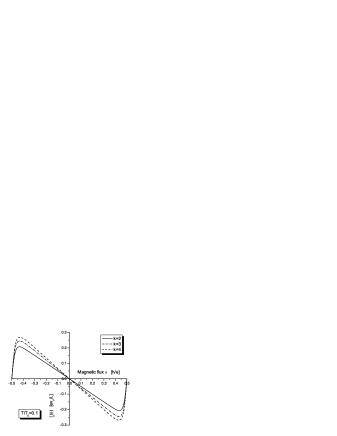
Figure 2: Persistent currents in the $k=2,3$ and $4$ parafermion FQH states, as functions of the magnetic flux within one period, computed numerically for $T/T_{0}=0.1$. The flux is measured in units $\mathrm{h}/\mathrm{e}$ and the current’s unit is $\mathrm{e}v_{F}/L$. The period is 1 flux quantum for all states and the amplitudes are $I_{2}^{\mathrm{max}}=0.207$, $I_{3}^{\mathrm{max}}=0.245$ and $I_{4}^{\mathrm{max}}=0.268$.

indicate that all currents are periodic in $\phi$ with period exactly $1$. We do not see any anomalous oscillations in the $k=2,3,4$ PF states, such as fractional flux periodicity of the persistent currents [10, 31, 32] which are characteristic for the BCS paired condensates, or more generally for some broken symmetries for all numerically accessible temperatures $0.03\leq T/T_{0}\leq 14$. This is a confirmation of the Bloch–Byers–Yang theorem [22] formulated in the context of superconductors. The persistent currents for the PF states have been shown to have oscillations for $M=0$ [32], however, this case is physically irrelevant. The case $M=0$ has only been used in [33] as a technical tool for investigating the wave functions for the PF states. One of the objectives of this paper was to show that the periods of the persistent currents for the PF states are exactly $1$ for all temperature. Nevertheless, for $T=0$ it is possible that the QH systems undergo phase transitions to some BCS-like phases where the periods could be less then $1$ due to some broken symmetries.

Furthermore, the amplitudes of the persistent currents in the parafermion FQH states decay exponentially with temperature, as shown in Fig. 3.

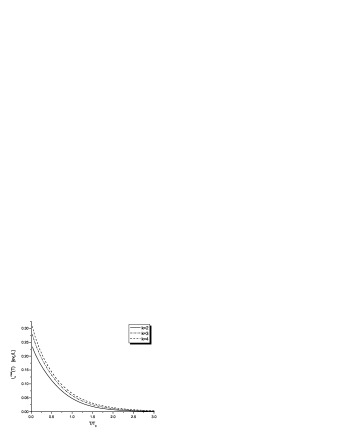
Figure 3: Temperature decay of the persistent current’s amplitudes in the $k=2,3$ and $4$ parafermion FQH states (without the contribution from the two $\nu=1$ Landau levels with opposite spins) computed numerically in units $\mathrm{e}v_{F}/L$, for temperatures measured in units of $T_{0}$. The zero temperature amplitude in these units are $\nu_{k}/2$, i.e., $1/4,3/10$ and $1/3$ respectively.

4.3 Low-temperature asymptotics of the persistent currents in the $\mathrm{PF}_{k}$ states

Because the low-temperature asymptotics of the chiral partition function (44) includes only universal parameters such as $\nu_{H}$, $Q_{\mathrm{qh}}$ and the proper quasihole energy $\widetilde{\varepsilon}_{\mathrm{qh}}$ the low-temperature behavior of the persistent current which we analyze in this section would have a universal form and would be valid for all FQH states.

Taking the logarithm of Eq. (44) and differentiating with respect to $\phi$ like in Eq. (68) we get the following expression for the persistent current for $|\phi|<1/2$

$$I(T,\phi)\ \mathop{=}_{T\ll T_{0}}\ \frac{\mathrm{e}v_{F}}{L}\left\{-\nu_{H}\phi+2Q_{\mathrm{qh}}\mathrm{e}^{-\frac{\widetilde{\varepsilon}_{\mathrm{qh}}}{k_{B}T}}\sinh\left(2\pi^{2}\frac{T_{0}}{T}Q_{\mathrm{qh}}\phi\right)\right\}.$$ (69)

4.3.1 The persistent current’s amplitude for $T=0$

For $T=0$ the second term in the curly brackets in Eq. (69) vanishes which expresses the fact that for zero temperature the free energy is determined by the ground state energy. Then the persistent current is simply proportional to the flux

$$I(T=0,\phi)=-\nu_{H}\,\frac{ev_{F}}{L}\,\phi,\quad\mathrm{for}\quad-\frac{1}{2}\leq\phi\leq\frac{1}{2},$$

which corresponds to the so called saw-tooth curve. It riches its maximum at $\phi=-1/2$ which is

$$I_{\mathrm{max}}=\frac{1}{2}\,\nu_{H}\,\frac{ev_{F}}{L}\quad\mathrm{for}\ T=0.$$

We stress that the zero temperature behavior of the persistent currents is completely determined by the CZ factors (36).

4.3.2 The persistent current’s amplitude for $0<T\ll T_{0}$

Because the persistent current is an odd periodic function of the flux we are going to consider the half-interval only $-1/2<\phi\leq 0$. Writing the $\sinh$ in Eq. (69) into its exponential form and ignoring $\exp(2\pi^{2}T_{0}Q_{\mathrm{qh}}\phi/T)$ which vanishes in the limit $T\to 0$ we get

$$I(T,\phi)\ \mathop{=}_{T\ll T_{0}}\ \frac{\mathrm{e}v_{F}}{L}\left\{-\nu_{H}\phi-Q_{\mathrm{qh}}\mathrm{e}^{-\frac{\widetilde{\varepsilon}_{\mathrm{qh}}}{k_{B}T}}\mathrm{e}^{-2\pi^{2}\frac{T_{0}}{T}Q_{\mathrm{qh}}\phi}\right\}.$$

The solution of $\partial I(T,\phi)/\partial\phi=0$ for $-1/2<\phi\leq 0$ gives the position of the current’s maximum

$$\phi_{\mathrm{max}}(T)\ \mathop{=}_{T\ll T_{0}}\ -\frac{\Delta_{\mathrm{qh}}}{Q_{\mathrm{qh}}}+\frac{1}{2\pi^{2}Q_{\mathrm{qh}}}\frac{T}{T_{0}}\ln\left(\frac{2\pi^{2}Q_{\mathrm{qh}}^{2}}{\nu_{H}}\frac{T_{0}}{T}\right)$$ (70)

and substituting Eq. (70) into Eq. (69) we get the following expression for the persistent current’s amplitude

$$I_{\mathrm{max}}(T)\ \mathop{=}_{T\ll T_{0}}\ \nu_{H}\frac{\mathrm{e}v_{F}}{L}\left\{\frac{\Delta_{\mathrm{qh}}}{Q_{\mathrm{qh}}}-\frac{1}{2\pi^{2}Q_{\mathrm{qh}}}\frac{T}{T_{0}}\left[1+\ln\left(\frac{2\pi^{2}Q_{\mathrm{qh}}^{2}}{\nu_{H}}\frac{T_{0}}{T}\right)\right]\right\}.$$ (71)

Using the charge–statistics relation Eq. (46) and the expression for the proper quasihole energy Eq. (45) we can rewrite Eq. (71) in the form of Eq. (47) according to which the persistent current’s amplitude decays logarithmically with increasing the temperature due to the thermal activation of quasiparticle–quasihole pairs.

4.4 High-temperature asymptotics of the persistent currents in the ${\mathbb{Z}}_{k}$ parafermion FQH states: extracting the universal decay exponents

Unlike the analysis of the low-temperature asymptotics of the persistent currents in Sect. 4.3 which has a universal form depending only on the quasiparticle charges and proper quasihole energies the high-temperature asymptotics, which is also universal, depends on the explicit form of the modular $S$ matrix so in the next subsections we shall illustrate it on the examples of the ${\mathbb{Z}}_{k}$ parafermion FQH states for $k=2,3$ and $4$. We show on Fig. 4 the logarithmic plot of the persistent currents amplitudes for the Fermi liquid with $\nu=1$, the Laughlin state with $\nu=1/3$ and the parafermion FQH states with $k=2,3$, and $4$ computed numerically from the corresponding CFT partition functions for temperature $0.03\leq T/T_{0}\leq 14$ which includes also the high-temperature regime $T\gg T_{0}$.

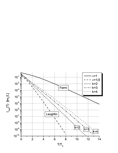
Figure 4: Logarithmic plot of the temperature decay of the persistent current’s amplitudes for the Fermi liquid ($\nu_{H}=1$), the Laughlin state ($\nu_{H}=1/3$) and the $k=2,3$ and $4$ parafermion FQH states

4.5 k=2

According to Eq. (57) the irreducible representations of the $\mathrm{PF}_{2}$ model are labelled by the pairs $(l,\rho)$ where $-1\leq l\leq 2$ and $\rho=0,1$ with the restriction $\rho\geq l-\rho\ \mathrm{mod}\ 2$. Using the explicit $S$ matrix for the Pfaffian FQH state from Ref. [34] (see Eq. (5.8) there) we find the universal coefficients necessary for the computation of the high-temperature limit of the partition function (50)

$$F^{l,\rho}=\sum_{l^{\prime}=-1}^{2}\ \sum_{\rho^{\prime}\geq l^{\prime}-\rho^{\prime}}S^{(l,\rho)}_{(l^{\prime},\rho^{\prime})}=\left\{\begin{array}[]{lcl}\sqrt{2}+1&\mathrm{for}&l=0,\ \rho=0\\ \sqrt{2}-1&\mathrm{for}&l=0,\ \rho=1\\ 0&&\mathrm{otherwise}\end{array}\right..$$

For convenience the characters of the $k=2$ parafermion FQH state are written explicitly in Eq. (A) and the chiral partition function (58) after $S$ transformation takes the form

$$Z_{2}(T,\phi) = (\sqrt{2}+1)\chi_{0,0}(\tau^{\prime},\zeta^{\prime})+(\sqrt{2}-1)\chi_{0,1}(\tau^{\prime},\zeta^{\prime})=$$ (72)

$$\simeq \left(\sqrt{2}+1\right)K_{0}(\tau^{\prime},2\zeta^{\prime};8)+\left(\sqrt{2}-1\right)K_{4}(\tau^{\prime},2\zeta^{\prime};8),$$

where we have dropped out a $\zeta^{\prime}$-independent term proportional to the central charge, substituted $\mathrm{ch}(\underline{\Lambda}_{0}+\underline{\Lambda}_{0})(\tau^{\prime})\simeq{q^{\prime}}^{0}$, $\mathrm{ch}(\underline{\Lambda}_{1}+\underline{\Lambda}_{1})(\tau^{\prime})\simeq{q^{\prime}}^{1/2}$ and ignored ${q^{\prime}}^{1/2}$ as compared to ${q^{\prime}}^{0}$ since $q^{\prime}\to 0$ when $T\to\infty$. Next, again dropping the $\eta$ function and taking only the leading terms in the $K$ functions, i.e., $n=0$ for $K_{0}(8)$ and $n=0,-1$ for $K_{4}(8)$ we get

$$Z_{2}(T,\phi)\ \mathop{\simeq}_{T\gg T_{0}}\ \left(\sqrt{2}+1\right)\left(1+2\left(\frac{\sqrt{2}-1}{\sqrt{2}+1}\right)q^{\prime}\cos(2\pi\zeta^{\prime})\right).$$

Substituting the $T$ and $\phi$ according to Eq. (48) and Eq. (49), using the approximation $\ln(1+X)\simeq X$ for $X\ll 1$ and taking the derivative with respect to $\phi$ according to Eq. (68) we get the following high-temperature asymptotic expression for the persistent current (note that $2\pi^{2}k_{B}T_{0}/\phi_{0}=ev_{F}/L$)

$$I_{2}(T,\phi)\mathop{\simeq}_{T\gg T_{0}}-I_{2}^{\mathrm{max}}(T)\sin(2\pi\phi),\quad I_{2}^{\mathrm{max}}(T)=\frac{ev_{F}}{L}\frac{2}{\pi}\left(\frac{\sqrt{2}-1}{\sqrt{2}+1}\right)\frac{T}{T_{0}}\exp\left(-2\frac{T}{T_{0}}\right)\quad$$ (73)

4.6 $k=3$

For this case Eq. (57) tells us that the irreducible representations are labelled by $(l,\rho)$ where $-2\leq l\leq 2$ and $0\leq\rho\leq 2$ with the restriction $\rho\geq l-\rho\ \mathrm{mod}\ 3$. The $S$ matrix has been written explicitly in Eq. (5.7) in Ref. [8] and the sums of the $S$-matrix elements are

$$F^{l,\rho}=\sum_{l^{\prime}=-2}^{2}\ \sum_{\rho^{\prime}\geq l^{\prime}-\rho^{\prime}}S^{(l,\rho)}_{(l^{\prime},\rho^{\prime})}=\left\{\begin{array}[]{rcl}\frac{2}{\sqrt{5}}\left(\sin\left(\frac{\pi}{5}\right)+3\sin\left(\frac{2\pi}{5}\right)\right)&\mathrm{for}&l=0,\ \rho=0\\ \frac{2}{\sqrt{5}}\left(3\sin\left(\frac{\pi}{5}\right)-\sin\left(\frac{2\pi}{5}\right)\right)&\mathrm{for}&l=0,\ \rho=2\\ 0&&\mathrm{otherwise}\end{array}\right..$$

The 10 independent characters in this case are shown in Eq. (A) and the partition function (58) for $k=3$ after $S$ transformation becomes

$$Z_{3}(T,\phi) = F^{0,0}\chi_{0,0}(\tau^{\prime},\zeta^{\prime})+F^{0,2}\chi_{0,2}(\tau^{\prime},\zeta^{\prime})\simeq$$

$$\simeq K_{0}(\tau^{\prime},3\zeta^{\prime};15)\left(F^{0,0}{q^{\prime}}^{0}+F^{0,2}{q^{\prime}}^{2/5}\right)+$$

$$+ K_{5}(\tau^{\prime},3\zeta^{\prime};15)\left(F^{0,0}{q^{\prime}}^{2/3}+F^{0,2}{q^{\prime}}^{1/15}\right)+$$

$$+ K_{-5}(\tau^{\prime},3\zeta^{\prime};15)\left(F^{0,0}{q^{\prime}}^{2/3}+F^{0,2}{q^{\prime}}^{1/15}\right),$$

where we have used $\mathrm{ch}(\underline{\Lambda}_{0}+\underline{\Lambda}_{0})(\tau^{\prime})\simeq{q^{\prime}}^{0}$, $\mathrm{ch}(\underline{\Lambda}_{0}+\underline{\Lambda}_{1})(\tau^{\prime})=\mathrm{ch}(\underline{\Lambda}_{0}+\underline{\Lambda}_{2})(\tau^{\prime})\simeq{q^{\prime}}^{1/15}$, $\mathrm{ch}(\underline{\Lambda}_{1}+\underline{\Lambda}_{1})(\tau^{\prime})=\mathrm{ch}(\underline{\Lambda}_{2}+\underline{\Lambda}_{2})(\tau^{\prime})\simeq{q^{\prime}}^{2/3}$ and $\mathrm{ch}(\underline{\Lambda}_{1}+\underline{\Lambda}_{2})(\tau^{\prime})\simeq{q^{\prime}}^{2/5}$ (using Eq. (56) for the CFT dimensions), again skipping the central charge term in the characters (60). Keeping only the lowest powers in $q^{\prime}\to 0$, ignoring the Dedekind function and taking only $n=0$ in the $K$ functions we get

$$Z_{3}(T,\phi)\ \mathop{\simeq}_{T\gg T_{0}}\ F^{0,0}\left(1+2\frac{F^{0,2}}{F^{0,0}}\,{q^{\prime}}^{\frac{1}{2}\left[5/3+2/15\right]}\cos(2\pi\zeta^{\prime})\right)$$

To get the persistent current in the high-temperature limit we apply the same scheme as for $k=2$ which yields

$$I_{3}(T,\phi) \ \mathop{\simeq}_{T\gg T_{0}}\ -I_{3}^{\mathrm{max}}(T)\sin(2\pi\phi),$$

$$I_{3}^{\mathrm{max}}(T) = \frac{ev_{F}}{L}\frac{2}{\pi}\left(\frac{D-1}{D+1}\right)\frac{T}{T_{0}}\exp\left(-\frac{T}{T_{0}}\left[\frac{5}{3}+\frac{2}{15}\right]\right),\quad$$ (74)

where we have used that

$$\frac{F^{0,2}}{F^{0,0}}=\frac{D-1}{D+1},\quad\mathrm{where}\quad D=2\cos\left(\frac{\pi}{5}\right)$$

is the quantum dimension of the elementary quasihole in the $\mathrm{PF}_{3}$ FQH state [8].

4.7 $k=4$

For $k=4$ the representations are labelled by (see Eq. (57)) $(l,\rho)$ where $-2\leq l\leq 3$ and $0\leq\rho\leq 3$ with the restriction $\rho\geq l-\rho\ \mathrm{mod}\ 4$. The 10 dimensional $S$ matrix ${{S}\raisebox{7.40005pt}{$\scriptscriptstyle\bullet$}\hskip 2.84544pt}$ for the (neutral) affine coset is shown in Eq. (95) and the complete 15 dimensional $S$ matrix is computed by Eq. (65). Then the sums of the $S$-matrix elements are

$$F^{l,\rho}=\sum_{l^{\prime}=-2}^{3}\ \sum_{\rho^{\prime}\geq l^{\prime}-\rho^{\prime}}S^{(l,\rho)}_{(l^{\prime},\rho^{\prime})}=\left\{\begin{array}[]{rcl}2+\sqrt{3}&\ \mathrm{for}&l=0,\ \rho=0\\ 2-\sqrt{3}&\ \mathrm{for}&l=0,\ \rho=2\\ 1&\ \mathrm{for}&l=0,\ \rho=3\\ 0&&\ \mathrm{otherwise}\end{array}\right.$$

so that the partition function (58) for $k=3$ becomes

$$Z_{4}(T,\phi) = F^{0,0}\chi_{0,0}(\tau^{\prime},\zeta^{\prime})+F^{0,2}\chi_{0,2}(\tau^{\prime},\zeta^{\prime})+F^{0,3}\chi_{0,3}(\tau^{\prime},\zeta^{\prime})\simeq$$

$$\simeq K_{0}(\tau^{\prime},4\zeta^{\prime};24)\left(F^{0,0}{q^{\prime}}^{\Delta^{\mathrm{PF}}(0,0)}+F^{0,2}{q^{\prime}}^{\Delta^{\mathrm{PF}}(2,2)}+F^{0,3}{q^{\prime}}^{\Delta^{\mathrm{PF}}(1,3)}\right)+$$

$$+ K_{6}(\tau^{\prime},4\zeta^{\prime};24)\left(F^{0,0}{q^{\prime}}^{\Delta^{\mathrm{PF}}(1,1)}+F^{0,2}{q^{\prime}}^{\Delta^{\mathrm{PF}}(3,3)}+F^{0,3}{q^{\prime}}^{\Delta^{\mathrm{PF}}(0,2)}\right)+$$

$$+ K_{-6}(\tau^{\prime},4\zeta^{\prime};24)\left(F^{0,0}{q^{\prime}}^{\Delta^{\mathrm{PF}}(3,3)}+F^{0,2}{q^{\prime}}^{\Delta^{\mathrm{PF}}(1,1)}+F^{0,3}{q^{\prime}}^{\Delta^{\mathrm{PF}}(0,2)}\right),$$

where the complete characters are shown in Eq. (A) and we have used $\mathrm{ch}(\underline{\Lambda}_{\mu}+\underline{\Lambda}_{\rho})(\tau^{\prime})\simeq{q^{\prime}}^{\Delta^{\mathrm{PF}}(\mu,\rho)}$, with $\Delta^{\mathrm{PF}}(0,0)=0$, $\Delta^{\mathrm{PF}}(0,2)=1/12$, $\Delta^{\mathrm{PF}}(1,1)=\Delta^{\mathrm{PF}}(3,3)=3/4$, $\Delta^{\mathrm{PF}}(1,3)=1/3$, $\Delta^{\mathrm{PF}}(2,2)=1$ (see Eq. (56) for the CFT dimensions $\Delta^{\mathrm{PF}}$), again skipping the central charge term in the characters (60). Keeping only the lowest powers in $q^{\prime}\to 0$, ignoring the Dedekind function and taking only $n=0$ in the $K$ functions we get

$$Z_{4}(T,\phi)\ \mathop{\simeq}_{T\gg T_{0}}\ F^{0,0}+2F^{0,3}{q^{\prime}}^{\frac{3}{4}+\Delta^{\mathrm{PF}}(0,2)}\cos(2\pi\zeta^{\prime})$$

To get the persistent current in the high-temperature limit we apply the same scheme as before

$$I_{4}(T,\phi) \ \mathop{\simeq}_{T\gg T_{0}}\ -I_{4}^{\mathrm{max}}(T)\sin(2\pi\phi),$$

$$I_{4}^{\mathrm{max}}(T) = \frac{ev_{F}}{L}\frac{2}{\pi}\left(\frac{1}{2+\sqrt{3}}\right)\frac{T}{T_{0}}\exp\left(-\frac{T}{T_{0}}\left[\frac{3}{2}+\frac{2}{12}\right]\right).$$ (75)

Finally, we can summarize the results for the high-temperature asymptotics of the persistent current’s amplitude for the $\mathrm{PF}_{k}$ FQH states

$$I^{\mathrm{max}}_{k}(T)\ \mathop{\simeq}_{T\gg T_{0}}\ I_{0}^{k}\,\left(\frac{T}{T_{0}}\right)\,\exp\left(-\alpha_{k}\frac{T}{T_{0}}\right)$$ (76)

where the exponent $\alpha_{k}$ for the ${\mathbb{Z}}_{k}$ parafermion FQH states is universal and can be written in general as

$$\alpha_{k}=\frac{1}{\nu_{H}}+2\Delta^{\mathrm{PF}}\left(\underline{\Lambda}_{0}+\underline{\Lambda}_{2}\right),\quad 2\Delta^{\mathrm{PF}}\left(\underline{\Lambda}_{0}+\underline{\Lambda}_{2}\right)=\frac{2(k-2)}{k(k+2)}.$$ (77)

Remark 4

While $\alpha=1/\nu_{H}$ for the Fermi and Laughlin states [3, 35], this exponent is not determined by the filling factor alone in the ${\mathbb{Z}}_{k}$ parafermion FQH states. Instead, there is a crucial contribution from the neutral sector which is described here by the ${\mathbb{Z}}_{k}$ parafermion coset.

The analysis of the high-temperature asymptotics allows us to predict the form of the universal exponents $\alpha$ for arbitrary FQH states. Because $F_{\lambda}\neq 0$ only if the corresponding electric charge $Q(\lambda)$ vanishes the neutral contribution to $\alpha$ would be determined from the neutral weight $\underline{\Lambda}_{*}$ with minimal neutral CFT dimension which satisfies the pairing rule with $l=d_{H}$, i.e.,

$$\alpha=\frac{1}{\nu_{H}}+2\Delta^{(0)}(\underline{\Lambda}_{*}),\quad\mathrm{where}\quad P[\underline{\Lambda}_{*}]\equiv d_{H}\ \mathrm{mod}\ k\quad\mathrm{with}\quad\Delta^{(0)}(\underline{\Lambda}_{*})=\min,$$ (78)

i.e., $\underline{\Lambda}_{*}$ is the lowest weight of the neutral character having the minimal CFT dimension among all neutral characters which couple to the ${\widehat{u(1)}}$ character $K_{\pm d_{H}}(\tau,n_{H}\zeta;n_{H}d_{H})$. Thus Eq. (77) should be valid for the entire parafermion hierarchy since $\underline{\Lambda}_{*}=\underline{\Lambda}_{0}+\underline{\Lambda}_{2}$ where $\Delta^{\mathrm{PF}}(\underline{\Lambda}_{0}+\underline{\Lambda}_{2})=\min$ is the minimal dimension of the weights satisfying the pairing rule $P[\underline{\Lambda}_{0}+\underline{\Lambda}_{2}]=2\equiv k+2\ \mathrm{mod}\ k$. Accidentally, the parafermion CFT dimension $\Delta^{\mathrm{PF}}(\underline{\Lambda}_{0}+\underline{\Lambda}_{2})=0$ for $k=2$ (see Eq. (56)) and the exponent in that case is given by the inverse of the filling factor only.

Using MAPLE we have computed the values of $\alpha$ and $I_{0}$ for the $k=2,3,4$ PF states from the numerical data shown on Fig. 4 by linear regression (after subtracting the $\ln(T/T_{0})$ contribution) over 80 points in the interval $6\leq T/T_{0}\leq 14$. The exact values of the exponents $\alpha$ and the (interpolated) asymptotic amplitudes $I_{0}$ for the first several $\mathrm{PF}_{k}$ states are in perfect agreement with the numerical ones and both are summarized in Table 1. The exponents $\alpha_{k}$ for the parafermion FQH states have to be compared with those corresponding to Fermi and Laughlin liquids which according to Remark 4 are $\alpha=1$ and $\alpha=3$ respectively.

Table 1: The slopes $\alpha$ and the $y$-intercepts $I_{0}$ (in units $\mathrm{e}v_{F}/L$) of the logarithmic plots in the high-temperature region for the $k=2,3,4$ PF states.

$k$	$\alpha$		$I_{0}$ $[\mathrm{e}v_{F}/L]$
	numeric	exact	numeric	exact
$2$	$2.000706$	$2$	$0.110253$	$(2/\pi)(\sqrt{2}-1)/(\sqrt{2}+1)$
$3$	$1.800010$	$1.8$	$0.150309$	$(2/\pi)(2\cos(\pi/5)-1)/(2\cos(\pi/5)+1)$
$4$	$1.666306$	$5/3$	$0.169827$	$(2/\pi)/(2+\sqrt{3})$

As mentioned before, Eq. (76) demonstrates that at high temperature there exists a different mechanism reducing the persistent currents – thermal decoherence which leads to exponential decay of the persistent currents amplitudes.

5 Conclusion

We have shown that the two-dimensional CFT for the edge states of a FQH disk sample can be effectively used to compute analytically the partition function in presence of Aharonov–Bohm flux. The effect of the AB flux is interpreted as twisting of the electron operator and of the CFT Hamiltonian leading to the very compact formula (34) for the partition function in presence of flux. Using this partition function as a thermodynamical potential one can compute the oscillating persistent current, AB magnetization and magnetic susceptibility in arbitrary FQH states. Because of the absence of complete spin–charge separation the excitations of the FQH liquid satisfy a ${\mathbb{Z}}_{n_{H}}$ pairing rule (22) that we have formulated in a general form. As a result we find that in general the CFT characters should have a specific ${\mathbb{Z}}_{n_{H}}$ invariant structure (23) of sum of products of charged and neutral characters. The general approach has been illustrated on the example of the parafermion FQH states in the second Landau level using the results of Ref. [8] for the corresponding CFT. Our analysis shows that the persistent currents in the parafermion FQH states are odd periodic functions of the AB flux with period exactly one flux quantum as it should be according to the Bloch–Byers–Yang theorem. We find that these currents are thermally suppressed by two different mechanisms in the low- and high- temperature limits, respectively and have universal non-Fermi liquid behavior.

For the high-temperature asymptotics of the parafermion CFT we have computed explicitly the modular $S$ matrices (65) using the convenient quasiparticle basis of Ref. [8]. As a byproduct we have derived the $S$ matrix (66) for the diagonal affine coset (53) in a very compact form and have proven that it is equivalent to the $S$ matrix of the $\widehat{su(k)}_{2}$ current algebra, i.e., not only the irreducible representations of the coset (53) and $\widehat{su(k)}_{2}$ are labelled by the same weights but the fusion rules of both CFTs are identical.

The universal exponents (77) extracted from the high-temperature asymptotics of the persistent currents show that for the FQH states with numerator of the filling factor $n_{H}>1$ there is always neutral contribution depending on the neutral sector and the ${\mathbb{Z}}_{n_{H}}$ pairing rule. The experimental measurement of these exponents may be useful for the identification of the correct CFT describing a given FQH universality class.

Appendix A Chiral partition functions for the parafermion QH states

For $k=2$ the $6$ independent characters entering Eq. (58) using the notation $K_{l}\left(8\right):=K_{l}\left(\tau,2\zeta;8\right)$ and $\mathrm{ch}(\mu,\rho):=\mathrm{ch}\left(\underline{\Lambda}_{\mu}+\underline{\Lambda}_{\rho}\right)(\tau)$ with $0\leq\mu\leq\rho\leq 1$ can be written

$$\chi_{-2,0}(\tau,\zeta) = K_{{-2}}\left(8\right)\mathrm{ch}\left({0},{0}\right)+K_{{2}}\left(8\right)\mathrm{ch}\left({1},{1}\right)$$

$$\chi_{-2,1}(\tau,\zeta) = K_{{-2}}\left(8\right)\mathrm{ch}\left({{1}},{{1}}\right)+K_{{2}}\left(8\right)\mathrm{ch}\left({0},{0}\right)$$

$$\chi_{-1,1}(\tau,\zeta) = K_{{-1}}\left(8\right)\mathrm{ch}\left({0},{1}\right)+K_{{3}}\left(8\right)\mathrm{ch}\left({0},{1}\right)$$

$$\chi_{0,0}(\tau,\zeta) = K_{{0}}\left(8\right)\mathrm{ch}\left({0},{0}\right)+K_{{4}}\left(8\right)\mathrm{ch}\left({1},{1}\right)$$

$$\chi_{0,1}(\tau,\zeta) = K_{{0}}\left(8\right)\mathrm{ch}\left({1},{1}\right)+K_{{4}}\left(8\right)\mathrm{ch}\left({0},{0}\right)$$

$$\chi_{1,1}(\tau,\zeta) = K_{{1}}\left(8\right)\mathrm{ch}\left({0},{1}\right)+K_{{-3}}\left(8\right)\mathrm{ch}\left({0},{1}\right)$$ (79)

For the $k=3$ parafermion state we use the following notation: $K_{l}\left(15\right):=K_{l}\left(\tau,3\zeta;15\right)$ and $\mathrm{ch}(\mu,\rho):=\mathrm{ch}\left(\underline{\Lambda}_{\mu}+\underline{\Lambda}_{\rho}\right)(\tau)$ with $0\leq\mu\leq\rho\leq 2$ the $10$ inequivalent characters are

$$\chi_{-2,1} = K_{{-2}}\left(15\right){\mathrm{ch}}\left(0,1\right)+K_{{3}}\left(15\right){\mathrm{ch}}\left(1,2\right)+K_{{-7}}\left(15\right){\mathrm{ch}}\left(0,2\right)$$

$$\chi_{-2,2} = K_{{-2}}\left(15\right){\mathrm{ch}}\left(2,2\right)+K_{{3}}\left(15\right){\mathrm{ch}}\left(0,0\right)+K_{{-7}}\left(15\right){\mathrm{ch}}\left(1,1\right)$$

$$\chi_{-1,1} = K_{{-1}}\left(15\right){\mathrm{ch}}\left(0,2\right)+K_{{4}}\left(15\right){\mathrm{ch}}\left(0,1\right)+K_{{-6}}\left(15\right){\mathrm{ch}}\left(1,2\right)$$

$$\chi_{-1,2} = K_{{-1}}\left(15\right){\mathrm{ch}}\left(1,1\right)+K_{{4}}\left(15\right){\mathrm{ch}}\left(2,2\right)+K_{{-6}}\left(15\right){\mathrm{ch}}\left(0,0\right)$$

$$\chi_{0,0} = K_{{0}}\left(15\right){\mathrm{ch}}\left(0,0\right)+K_{{5}}\left(15\right){\mathrm{ch}}\left(1,1\right)+K_{{-5}}\left(15\right){\mathrm{ch}}\left(2,2\right)$$

$$\chi_{0,2} = K_{{0}}\left(15\right){\mathrm{ch}}\left(1,2\right)+K_{{5}}\left(15\right){\mathrm{ch}}\left(0,2\right)+K_{{-5}}\left(15\right){\mathrm{ch}}\left(0,1\right)$$

$$\chi_{1,1} = K_{{1}}\left(15\right){\mathrm{ch}}\left(0,1\right)+K_{{6}}\left(15\right){\mathrm{ch}}\left(1,2\right)+K_{{-4}}\left(15\right){\mathrm{ch}}\left(0,2\right)$$

$$\chi_{1,2} = K_{{1}}\left(15\right){\mathrm{ch}}\left(2,2\right)+K_{{6}}\left(15\right){\mathrm{ch}}\left(0,0\right)+K_{{-4}}\left(15\right){\mathrm{ch}}\left(1,1\right)$$

$$\chi_{2,1} = K_{{2}}\left(15\right){\mathrm{ch}}\left(0,2\right)+K_{{7}}\left(15\right){\mathrm{ch}}\left(0,1\right)+K_{{-3}}\left(15\right){\mathrm{ch}}\left(1,2\right)$$

$$\chi_{2,2} = K_{{2}}\left(15\right){\mathrm{ch}}\left(1,1\right)+K_{{7}}\left(15\right){\mathrm{ch}}\left(2,2\right)+K_{{-3}}\left(15\right){\mathrm{ch}}\left(0,0\right)$$ (80)

For $k=4$ parafermion state where $K_{l}\left(24\right):=K_{l}\left(\tau,4\zeta;24\right)$ and $\mathrm{ch}(\mu,\rho):=\mathrm{ch}\left(\underline{\Lambda}_{\mu}+\underline{\Lambda}_{\rho}\right)(\tau)$ with $0\leq\mu\leq\rho\leq 3$ we have $15$ independent characters

$$\chi_{-3,1} = K_{{-3}}\left(24\right)\mathrm{ch}\left(0,1\right)+K_{{3}}\left(24\right)\mathrm{ch}\left(1,2\right)+K_{{9}}\left(24\right)\mathrm{ch}\left(2,3\right)+K_{{-9}}\left(24\right)\mathrm{ch}\left(0,3\right)$$

$$\chi_{-3,3} = K_{{-3}}\left(24\right)\mathrm{ch}\left(2,3\right)+K_{{3}}\left(24\right)\mathrm{ch}\left(0,3\right)+K_{{9}}\left(24\right)\mathrm{ch}\left(0,1\right)+K_{{-9}}\left(24\right)\mathrm{ch}\left(1,2\right)$$

$$\chi_{-2,1} = K_{{-2}}\left(24\right)\mathrm{ch}\left(0,2\right)+K_{{4}}\left(24\right)\mathrm{ch}\left(1,3\right)+K_{{10}}\left(24\right)\mathrm{ch}\left(0,2\right)+K_{{-8}}\left(24\right)\mathrm{ch}\left(1,3\right)$$

$$\chi_{-2,2} = K_{{-2}}\left(24\right)\mathrm{ch}\left(1,1\right)+K_{{4}}\left(24\right)\mathrm{ch}\left(2,2\right)+K_{{10}}\left(24\right)\mathrm{ch}\left(3,3\right)+K_{{-8}}\left(24\right)\mathrm{ch}\left(0,0\right)$$

$$\chi_{-2,3} = K_{{-2}}\left(24\right)\mathrm{ch}\left(3,3\right)+K_{{4}}\left(24\right)\mathrm{ch}\left(0,0\right)+K_{{10}}\left(24\right)\mathrm{ch}\left(1,1\right)+K_{{-8}}\left(24\right)\mathrm{ch}\left(2,2\right)$$

$$\chi_{-1,2} = K_{{-1}}\left(24\right)\mathrm{ch}\left(0,3\right)+K_{{5}}\left(24\right)\mathrm{ch}\left(0,1\right)+K_{{11}}\left(24\right)\mathrm{ch}\left(1,2\right)+K_{{-7}}\left(24\right)\mathrm{ch}\left(2,3\right)$$

$$\chi_{-1,3} = K_{{-1}}\left(24\right)\mathrm{ch}\left(1,2\right)+K_{{5}}\left(24\right)\mathrm{ch}\left(2,3\right)+K_{{11}}\left(24\right)\mathrm{ch}\left(0,3\right)+K_{{-7}}\left(24\right)\mathrm{ch}\left(0,1\right)$$

$$\chi_{0,0} = K_{{0}}\left(24\right)\mathrm{ch}\left(0,0\right)+K_{{6}}\left(24\right)\mathrm{ch}\left(1,1\right)+K_{{12}}\left(24\right){\mathrm{ch}}\left(2,2\right)+K_{{-6}}\left(24\right)\mathrm{ch}\left(3,3\right)$$

$$\chi_{0,2} = K_{{0}}\left(24\right)\mathrm{ch}\left(1,3\right)+K_{{6}}\left(24\right)\mathrm{ch}\left(0,2\right)+K_{{12}}\left(24\right){\mathrm{ch}}\left(1,3\right)+K_{{-6}}\left(24\right)\mathrm{ch}\left(0,2\right)$$

$$\chi_{0,3} = K_{{0}}\left(24\right)\mathrm{ch}\left(2,2\right)+K_{{6}}\left(24\right)\mathrm{ch}\left(3,3\right)+K_{{12}}\left(24\right){\mathrm{ch}}\left(0,0\right)+K_{{-6}}\left(24\right)\mathrm{ch}\left(1,1\right)$$

$$\chi_{1,1} = K_{{1}}\left(24\right)\mathrm{ch}\left(0,1\right)+K_{{7}}\left(24\right)\mathrm{ch}\left(1,2\right)+K_{{-11}}\left(24\right){\mathrm{ch}}\left(2,3\right)+K_{{-5}}\left(24\right)\mathrm{ch}\left(0,3\right)$$

$$\chi_{1,3} = K_{{1}}\left(24\right)\mathrm{ch}\left(2,3\right)+K_{{7}}\left(24\right)\mathrm{ch}\left(0,3\right)+K_{{-11}}\left(24\right){\mathrm{ch}}\left(0,1\right)+K_{{-5}}\left(24\right)\mathrm{ch}\left(1,2\right)$$

$$\chi_{2,1} = K_{{2}}\left(24\right)\mathrm{ch}\left(0,2\right)+K_{{8}}\left(24\right)\mathrm{ch}\left(1,3\right)+K_{{-10}}\left(24\right){\mathrm{ch}}\left(0,2\right)+K_{{-4}}\left(24\right)\mathrm{ch}\left(1,3\right)$$

$$\chi_{2,2} = K_{{2}}\left(24\right)\mathrm{ch}\left(1,1\right)+K_{{8}}\left(24\right)\mathrm{ch}\left(2,2\right)+K_{{-10}}\left(24\right){\mathrm{ch}}\left(3,3\right)+K_{{-4}}\left(24\right)\mathrm{ch}\left(0,0\right)$$

$$\chi_{2,3} = K_{{2}}\left(24\right)\mathrm{ch}\left(3,3\right)+K_{{8}}\left(24\right)\mathrm{ch}\left(0,0\right)+K_{{-10}}\left(24\right){\mathrm{ch}}\left(1,1\right)+K_{{-4}}\left(24\right)\mathrm{ch}\left(2,2\right)$$

Appendix B The diagonal coset’s $S$ matrix

In this appendix we shall sketch the derivation of the modular $S$ matrix for the coset (53) following the general approach of Goddard–Kent–Olive [26]. The characters of the diagonal coset appear by definition as string functions in the decomposition of the coset numerator $\widehat{su(k)}_{1}\oplus\widehat{su(k)}_{1}$ in terms of the $\widehat{su(k)}_{2}$ characters

$$\chi_{\Lambda}^{(1)}(\tau)\ \chi_{\Lambda^{\prime}}^{(1)}(\tau)=\sum_{\Lambda^{\prime\prime}}\ P(\Lambda,\Lambda^{\prime};\Lambda^{\prime\prime})\ \mathrm{ch}{\scriptsize\left(\begin{array}[]{c}\Lambda\ ,\ \Lambda^{\prime}\\ \Lambda^{\prime\prime}\end{array}\right)}(\tau)\ \chi_{\Lambda^{\prime\prime}}^{(2)}(\tau),$$ (82)

where $\chi_{\Lambda}^{(1)}$ and $\chi_{\Lambda}^{(2)}$ are the $\widehat{su(k)}_{l}$ characters at level $l=1$ and $2$ respectively and the function

$$P(\Lambda,\Lambda^{\prime};\Lambda^{\prime\prime})=\left\{\begin{array}[]{cl}1&\quad\mathrm{if}\quad[\Lambda^{\prime\prime}]=[\Lambda]+[\Lambda^{\prime}]\\ 0&\quad\mathrm{otherwise}\end{array}\right.$$

expresses the ${\mathbb{Z}}_{k}$ charge conservation rule [17]. Let us now apply the $S$ transformation $\tau\to-1/\tau$ to both sides, i.e., $S\chi_{\Lambda}^{(1)}=\sum_{\mu}S^{(1)}_{\Lambda,\mu}\chi_{\mu}^{(1)}$, $S\chi_{\Lambda^{\prime}}^{(1)}=\sum_{\mu^{\prime}}S^{(1)}_{\Lambda^{\prime},\mu^{\prime}}\chi_{\mu^{\prime}}^{(1)}$ $S\chi_{\Lambda^{\prime\prime}}^{(2)}=\sum_{\sigma}S^{(2)}_{\Lambda^{\prime\prime},\sigma}\chi_{\sigma}^{(2)}$ and $S\mathrm{ch}_{\rho^{\prime\prime}}=\sum_{\rho^{\prime\prime}}{{S}\raisebox{7.40005pt}{$\scriptscriptstyle\bullet$}\hskip 2.84544pt}^{\Lambda^{\prime\prime}}_{\rho^{\prime\prime}}\mathrm{ch}_{\rho^{\prime\prime}}$ and then decompose again the product $\chi_{\mu}^{(1)}(\tau)\chi_{\mu^{\prime}}^{(1)}(\tau)$ in the left hand side in terms of the $\chi_{\mu^{\prime\prime}}^{(2)}$ and the coset characters using Eq. (82)

$$\sum_{\mu,\mu^{\prime}\ \mathrm{mod}\ k}\ \sum_{\mu^{\prime\prime}}P(\mu,\mu^{\prime};\mu^{\prime\prime})S^{(1)}_{\Lambda,\mu}S^{(1)}_{\Lambda^{\prime},\mu^{\prime}}\ \mathrm{ch}\left(\scriptsize\begin{array}[]{c}\mu\ ,\ \mu^{\prime}\\ \mu^{\prime\prime}\end{array}\right)(\tau)\ \chi_{\mu^{\prime\prime}}^{(2)}(\tau)=$$ (85)

$$=\sum_{\Lambda^{\prime\prime}}P(\Lambda,\Lambda^{\prime};\Lambda^{\prime\prime})\sum_{\rho^{\prime\prime}}\sum_{\sigma}{{S}\raisebox{7.40005pt}{$\scriptscriptstyle\bullet$}\hskip 2.84544pt}^{\Lambda^{\prime\prime}}_{\rho^{\prime\prime}}S^{(2)}_{\Lambda^{\prime\prime},\sigma}\mathrm{ch}\left(\scriptsize\begin{array}[]{c}[\rho^{\prime\prime}]\ ,\ 0\\ \rho^{\prime\prime}\end{array}\right)(\tau)\ \chi_{\sigma}^{(2)}(\tau),$$ (88)

where we have used the triple equivalence to label the coset representations by the level-2 index only. Next we substitute $\sigma=\mu^{\prime\prime}$ in the RHS, compare the coefficients of $\chi_{\mu^{\prime\prime}}^{(2)}$, multiply both sides by $(S^{(2)}_{\mu^{\prime\prime},\nu})^{-1}$ and sum over $\mu^{\prime\prime}$ to get

$$\sum_{\mu,\mu^{\prime}\ \mathrm{mod}\ k}\ \sum_{\mu^{\prime\prime}}P(\mu,\mu^{\prime};\mu^{\prime\prime})S^{(1)}_{\Lambda,\mu}S^{(1)}_{\Lambda^{\prime},\mu^{\prime}}\ (S^{(2)}_{\mu^{\prime\prime},\nu})^{-1}\mathrm{ch}\left(\scriptsize\begin{array}[]{c}\mu\ ,\ \mu^{\prime}\\ \mu^{\prime\prime}\end{array}\right)(\tau)=$$ (91)

$$=P(\Lambda,\Lambda^{\prime};\nu)\sum_{\rho^{\prime\prime}}{{S}\raisebox{7.40005pt}{$\scriptscriptstyle\bullet$}\hskip 2.84544pt}^{\nu}_{\rho^{\prime\prime}}\mathrm{ch}\left(\scriptsize\begin{array}[]{c}[\rho^{\prime\prime}]\ ,\ 0\\ \rho^{\prime\prime}\end{array}\right)(\tau).$$ (94)

Because $(\mu,\mu^{\prime};\mu^{\prime\prime})\stackrel{{\scriptstyle\mathrm{def}}}{{=}}\ (\underline{\Lambda}_{\mu},\underline{\Lambda}_{\mu^{\prime}};\underline{\Lambda}_{\alpha}+\underline{\Lambda}_{\beta})$ we can shift the summation variables in the LHS according to

$$\mu=\widetilde{\mu}+\mu^{\prime},\quad\alpha=\widetilde{\alpha}+\mu^{\prime},\quad\beta=\widetilde{\beta}+\mu^{\prime}$$

and use the triples equivalence $(\underline{\Lambda}_{\mu},\underline{\Lambda}_{\mu^{\prime}};\underline{\Lambda}_{\alpha}+\underline{\Lambda}_{\beta})\equiv(\underline{\Lambda}_{\widetilde{\mu}},0;\underline{\Lambda}_{\widetilde{\alpha}}+\underline{\Lambda}_{\widetilde{\beta}})$ to get for the LHS

$$\sum_{\mu^{\prime}\ \mathrm{mod}\ k}\ \sum_{\widetilde{\mu}\ \mathrm{mod}\ k}\sum_{\widetilde{\alpha}\leq\widetilde{\beta}}P(\widetilde{\mu},0;\widetilde{\alpha}+\widetilde{\beta})\,S^{(1)}_{\Lambda,\widetilde{\mu}+\mu^{\prime}}S^{(1)}_{\Lambda^{\prime},\mu^{\prime}}\ (S^{(2)}_{\widetilde{\alpha}+\mu^{\prime}+\widetilde{\beta}+\mu^{\prime},\nu})^{-1}\,\mathrm{ch}\left(\scriptsize\begin{array}[]{c}\widetilde{\mu}\ ,\ 0\\ \widetilde{\alpha}+\widetilde{\beta}\end{array}\right)(\tau),$$

where we have used that $P(\widetilde{\mu}+\mu^{\prime},\mu^{\prime};\widetilde{\alpha}+\mu^{\prime}+\widetilde{\beta}+\mu^{\prime})=P(\widetilde{\mu},0;\widetilde{\alpha}+\widetilde{\beta})$. Now we can use the properties of the $S$ matrices under the action of simple currents

$$S^{(1)}_{\Lambda,\widetilde{\mu}+\mu^{\prime}}=\mathrm{e}^{2\pi i\frac{\mu^{\prime}\Lambda}{k}}S^{(1)}_{\Lambda,\widetilde{\mu}},\quad S^{(1)}_{\Lambda^{\prime},\mu^{\prime}}=\mathrm{e}^{2\pi i\frac{\mu^{\prime}\Lambda^{\prime}}{k}}S^{(1)}_{\Lambda^{\prime},0},\quad S^{(2)}_{\Lambda_{\widetilde{\alpha}+\mu^{\prime}}+\Lambda_{\widetilde{\beta}+\mu^{\prime}}}=\mathrm{e}^{-2\pi iQ^{(2)}_{\mathcal{J}^{\mu^{\prime}}}(\nu)}S^{(2)}_{\Lambda_{\widetilde{\alpha}}+\Lambda_{\widetilde{\beta}},\nu},$$

where $Q^{(2)}_{\mathcal{J}^{\mu^{\prime}}}(\nu)$ is the monodromy charge (62) in the $\widehat{su(k)}_{2}$ CFT. Writing the $\widehat{su(k)}_{2}$ weight $\nu=\underline{\Lambda}_{\rho}+\underline{\Lambda}_{\sigma}$ with $0\leq\rho\leq\sigma\leq k-1$ and using the following formula for the CFT dimensions in $\widehat{su(k)}_{2}$

$$\Delta^{(2)}(\underline{\Lambda}_{\rho}+\underline{\Lambda}_{\sigma})=\frac{2\rho(k-\sigma)+(k+1)\left[\rho(k-\rho)+\sigma(k-\sigma)\right]}{2k(k+2)}$$

we get the following simple expression for the monodromy charge

$$Q^{(2)}_{\mathcal{J}^{\mu^{\prime}}}(\underline{\Lambda}_{\rho}+\underline{\Lambda}_{\sigma})=-\frac{\mu^{\prime}(\rho+\sigma)}{k}.$$

The final step is to take the summation over $\mu^{\prime}$ using again the $\delta$-function

$$\sum_{\mu^{\prime}\ \mathrm{mod}\ k}\exp\left(2\pi i\,\frac{\mu^{\prime}\left[\Lambda+\Lambda^{\prime}-(\rho+\sigma)\right]}{k}\right)=k\,P(\Lambda,\Lambda^{\prime};\nu),$$

set $\rho^{\prime\prime}=\Lambda_{\widetilde{\alpha}}+\Lambda_{\widetilde{\beta}}$ (then $\widetilde{\mu}=\underline{\Lambda}_{[\rho^{\prime\prime}]}=:[\rho^{\prime\prime}]$ due to the conservation of the ${\mathbb{Z}}_{k}$ charge in the coset) and compare the coefficients of $\mathrm{ch}{\scriptsize\left(\begin{array}[]{c}[\rho^{\prime\prime}]\ ,\ 0\\ \rho^{\prime\prime}\end{array}\right)}(\tau)$ which gives the coset $S$ matrix, Eq. (66).

For the high-temperature asymptotics of the persistent current in the $k=4$ parafermion FQH state we shall need the (neutral) $S$ matrix (66). Using the following basis of $10$ coset weights

$$\underline{\Lambda}_{0}+\underline{\Lambda}_{0}, \quad\underline{\Lambda}_{0}+\underline{\Lambda}_{1},\quad\underline{\Lambda}_{0}+\underline{\Lambda}_{2},\quad\underline{\Lambda}_{0}+\underline{\Lambda}_{3},\quad\underline{\Lambda}_{1}+\underline{\Lambda}_{1},$$

$$\underline{\Lambda}_{1}+\underline{\Lambda}_{2}, \quad\underline{\Lambda}_{1}+\underline{\Lambda}_{3},\quad\underline{\Lambda}_{2}+\underline{\Lambda}_{2},\quad\underline{\Lambda}_{2}+\underline{\Lambda}_{3},\quad\underline{\Lambda}_{3}+\underline{\Lambda}_{3},$$

the matrix ${{S}\raisebox{7.40005pt}{$\scriptscriptstyle\bullet$}\hskip 2.84544pt}^{\mu,\nu}_{\rho,\sigma}$ has been computed with Maple by Eq. (66) where the $S$ matrix of the denominator $\widehat{su(4)}_{2}$ of the coset has been computed by the Kac formula (67)

$$\left[{{S}\raisebox{7.40005pt}{$\scriptscriptstyle\bullet$}\hskip 2.84544pt}^{\mu,\nu}_{\rho,\sigma}\right]=\left[\begin{array}[]{cccccccccc}\frac{\sqrt{6}}{12}&\frac{\sqrt{2}}{4}&\frac{\sqrt{6}}{6}&\frac{\sqrt{2}}{4}&\frac{\sqrt{6}}{12}&\frac{\sqrt{2}}{4}&\frac{\sqrt{6}}{6}&\frac{\sqrt{6}}{12}&\frac{\sqrt{2}}{4}&\frac{\sqrt{6}}{12}\\ \frac{\sqrt{2}}{4}&\frac{1+i}{4}&0&\frac{1-i}{4}&\frac{i\sqrt{2}}{4}&\frac{-1+i}{4}&0&\frac{-\sqrt{2}}{4}&\frac{-1-i}{4}&\frac{-i\sqrt{2}}{4}\\ \frac{\sqrt{6}}{6}&0&\frac{\sqrt{6}}{6}&0&\frac{-\sqrt{6}}{6}&0&\frac{-\sqrt{6}}{6}&\frac{\sqrt{6}}{6}&0&\frac{-\sqrt{6}}{6}\\ \frac{\sqrt{2}}{4}&\frac{1-i}{4}&0&\frac{1+i}{4}&\frac{-i\sqrt{2}}{4}&\frac{-1-i}{4}&0&\frac{-\sqrt{2}}{4}&\frac{-1+i}{4}&\frac{i\sqrt{2}}{4}\\ \frac{\sqrt{6}}{12}&\frac{i\sqrt{2}}{4}&\frac{-\sqrt{6}}{6}&\frac{-i\sqrt{2}}{4}&\frac{-\sqrt{6}}{12}&\frac{-i\sqrt{2}}{4}&\frac{\sqrt{6}}{6}&\frac{\sqrt{6}}{12}&\frac{i\sqrt{2}}{4}&\frac{-\sqrt{6}}{12}\\ \frac{\sqrt{2}}{4}&\frac{-1+i}{4}&0&\frac{-1-i}{4}&\frac{-i\sqrt{2}}{4}&\frac{1+i}{4}&0&\frac{-\sqrt{2}}{4}&\frac{1-i}{4}&\frac{i\sqrt{2}}{4}\\ \frac{\sqrt{6}}{6}&0&\frac{-\sqrt{6}}{6}&0&\frac{\sqrt{6}}{6}&0&\frac{-\sqrt{6}}{6}&\frac{\sqrt{6}}{6}&0&\frac{\sqrt{6}}{6}\\ \frac{\sqrt{6}}{12}&\frac{-\sqrt{2}}{4}&\frac{\sqrt{6}}{6}&\frac{-\sqrt{2}}{4}&\frac{\sqrt{6}}{12}&\frac{-\sqrt{2}}{4}&\frac{\sqrt{6}}{6}&\frac{\sqrt{6}}{12}&\frac{-\sqrt{2}}{4}&\frac{\sqrt{6}}{12}\\ \frac{\sqrt{2}}{4}&\frac{-1-i}{4}&0&\frac{-1+i}{4}&\frac{i\sqrt{2}}{4}&\frac{1-i}{4}&0&\frac{-\sqrt{2}}{4}&\frac{1+i}{4}&\frac{-i\sqrt{2}}{4}\\ \frac{\sqrt{6}}{12}&\frac{-i\sqrt{2}}{4}&\frac{-\sqrt{6}}{6}&\frac{i\sqrt{2}}{4}&\frac{-\sqrt{6}}{12}&\frac{i\sqrt{2}}{4}&\frac{\sqrt{6}}{6}&\frac{\sqrt{6}}{12}&\frac{-i\sqrt{2}}{4}&\frac{-\sqrt{6}}{12}\\ \end{array}\right]$$ (95)

References

• [1] D. Mailly, C. Chapelier, and A. Benoit, “Experimental observation of persistent currents in a GaAs-AlGaAs single loop,” Phys. Rev. Lett. 70 (1993) 2020.
• [2] J. Fröhlich, U. M. Studer, and E. Thiran, “A classification of quantum Hall fluids,” J. Stat. Phys. 86 (1997) 821, cond-mat/9503113.
• [3] M. Geller, D. Loss, and G. Kirczenow, “Mesoscopic effects in the fractional quantum Hall regime: chiral Luttinger liquid versus Fermi liquid,” Phys. Rev. Lett. 77 (1996) 49.
• [4] M. Geller and D. Loss, “Aharonov–Bohm effect in the chiral Luttinger liquid,” Phys. Rev. B 56 (1997) 9692.
• [5] M. Grayson, D. Tsui, L. Pfeiffer, K. West, and A. Chang, “Continuum of chiral Luttinger liquids at the fractional quantum Hall edge,” Phys. Rev. Lett. 80 (1998) 1062.
• [6] L. Georgiev, “The $\nu=5/2$ quantum Hall state revisited: spontaneous breaking of the chiral fermion parity and phase transition between abelian and non-abelian statistics,” Nucl. Phys. B 651 (2003) 331–360, hep-th/0108173.
• [7] L. Georgiev, “Chiral persistent currents and magnetic susceptibilities in the parafermion quantum Hall states in the second Landau level with Aharonov–Bohm flux,” Phys. Rev. B 69 (2004) 085305, cond-mat/0311339.
• [8] A. Cappelli, L. Georgiev, and I. Todorov, “Parafermion Hall states from coset projections of abelian conformal theories,” Nucl. Phys. B 599 [FS] (2001) 499–530, hep-th/0009229.
• [9] L. Georgiev and M. Geller, “Magnetic moment oscillations in a quantum Hall ring,” (2004) cond-mat/0404681.
• [10] K. Ino, “Pairing effects at the edge of paired quantum Hall states,” Phys. Rev. Lett. 81 (1998) 1078, cond-mat/9803337.
• [11] J. Fröhlich, B. Pedrini, C. Schweigert, and J. Walcher, “Universality in quantum Hall systems: Coset construction of incompressible states,” J. Stat. Phys. 103 (2001) 527, cond-mat/0002330.
• [12] X.-G. Wen Adv. Phys. 44 (1995) 405.
• [13] L. Georgiev, “Stability and activation gaps of parafermionic Hall states in the second Landau level,” Nucl. Phys. B 626 (2002) 415–434, cond-mat/0102451.
• [14] A. Cappelli and G. R. Zemba, “Modular invariant partition functions in the quantum Hall effect,” Nucl. Phys. B490 (1997) 595, hep-th/9605127.
• [15] P. Di Francesco, P. Mathieu, and D. Sénéchal, Conformal Field Theory. Springer–Verlag, New York, 1997.
• [16] A. Cappelli, C. Trugenberger, and G. Zemba, “$w_{1+\infty}$ dynamics of edge excitations in the quantum Hall effect,” Annals Phys. 246 (1996) 86, cond-mat/9407095.
• [17] J. Fuchs, B. Schellekens, and C. Schweigert, “The resolution of field identification fixed points in diagonal coset theories,” Nucl. Phys. B461 (1996) 371, hep-th/9509105.
• [18] V. Kac and I. Todorov Commun. Math Phys. 190 (1997) 57–111.
• [19] L. Georgiev and I. Todorov, “RCFT extensions of $W_{1+\infty}$ in terms of bilocal fields,” J. Math. Phys. 39 (1998) 5762–5771, hep-th/9710134.
• [20] A. Cappelli, C. A. Trugenberger, and G. R. Zemba Nucl. Phys. B396 (1993) 465.
• [21] R. Laughlin, “Anomalous quantum Hall effect: An incompressible quantum fluid with fractionally charged excitations,” Phys. Rev. Lett. 50 (1983) 1395.
• [22] N. Byers and C. Yang, “Theoretical considerations concerning quantized magnetic flux in superconducting cylinders,” Phys. Rev. Lett. 7 (1961) 46.
• [23] M. Halpern Ann. of Phys. 194 (1989) 247.
• [24] M. Halpern, E. Kiritsis, N. Obers, and K. Clubok, “Irrational conformal field theory,” Phys. Rept. 265 (1996) 1–138, hep-th/9501144.
• [25] G. Cristofano, G. Maiella, and V. Marotta, “A conformal field theory description of the paired and parafermionic states in the quantum Hall effect,” Mod. Phys. Lett. A 15 (2000) 1679.
• [26] P. Goddard, A. Kent, and D. Olive Commun. Math. Phys. 103 (1986) 105.
• [27] V. Kac, Infinite Dimensional Lie Algebras. Cambridge University Press, Cambridge, second ed., 1985.
• [28] L. Georgiev, “The diagonal affine coset construction of the ${{\mathbb{Z}}}_{k}$ parafermion Hall states,” proc. of the Fifth Int. Workshop ”Lie Theory and its Applications in Physics”, Eds. V. Dobrev et al., World Scientific, Singapore (2004) hep-th/0402159.
• [29] S. Coleman Commun. Math. Phys. 31 (1973) 259.
• [30] N. Mermin and H. Wagner, “Absence of feromagnetism in one- and two- dimensional isotropic Heisenberg models,” Phys. Rev. Lett. 17 (1966) 1133.
• [31] K. Ino, “Persistent edge currents for paired quantum Hall states,” Phys. Rev. B62 (2000) 6936, cond-mat/0008094.
• [32] H. Kiryu, “Oscillations of persistent edge currents in the parafermion quantum Hall states,” Phys. Rev. B65 (2002) 113407.
• [33] N. Read and E. Rezayi Phys. Rev. B59 (1998) 8084.
• [34] A. Cappelli, L. Georgiev, and I. Todorov, “A unified conformal field theory approach to paired quantum Hall states,” Commun. Math. Phys. 205 (1999) 657–689, preprint ESI-621 (1998); hep-th/9810105.
• [35] M. Geller, D. Loss, and G. Kirczenow, “Luttinger liquids and composite fermions in nanostructures: what is the nature of the edge states in the fractional quantum Hall effect?,” Superlattices Microstruct. 21 (1997) 5110.