Abstract

Type 0A string theory in the $(2,4k)$ superconformal minimal model backgrounds and the bosonic string in the $(2,2k-1)$ conformal minimal models, while perturbatively identical in some regimes, may be distinguished non–perturbatively using double scaled matrix models. The resolvent of an associated Schrödinger operator plays three very important interconnected roles, which we explore perturbatively and non–perturbatively. On one hand, it acts as a source for placing D–branes and fluxes into the background, while on the other, it acts as a probe of the background, its first integral yielding the effective force on a scaled eigenvalue. We study this probe at disc, torus and annulus order in perturbation theory, in order to characterize the effects of D–branes and fluxes on the matrix eigenvalues. On a third hand, the integrated resolvent forms a representation of a twisted boson in an associated conformal field theory. The entire content of the closed string theory can be expressed in terms of Virasoro constraints on the partition function, which is realized as wavefunction in a coherent state of the boson. Remarkably, the D–brane or flux background is simply prepared by acting with a vertex operator of the twisted boson. This generates a number of sharp examples of open–closed duality, both old and new. We discuss whether the twisted boson conformal field theory can usefully be thought of as another holographic dual of the non–critical string theory.

1 Introduction and Discussion

In recent years, it has become clear that the separation between open and closed string descriptions of certain physical phenomena is very much an artifact of perturbation theory. This means more than just strong/weak coupling dualities linking different string theories, but also includes transitions within a given theory from an open string description (e.g., involving D–branes) to a closed string one (e.g., involving only fluxes), as the strength of a coupling changes. Gauge/string dualities are the best known examples of this type of phenomenon, and for that reason alone it is of interest to learn more about how to describe them. For this, it is of course necessary to go beyond perturbation theory, and furthermore, to develop a far richer picture than that which is accessible using only simple strong/weak coupling duality. We need to be able to define the theories in question at arbitrary values of the couplings in order to address the many subtle issues which can arise.

Matrix models in the double scaling limit[1, 2, 3] defined for us the earliest examples of exactly solvable string theories with readily accessible non–perturbative information. These types of models have recently been interpreted as examples of open/closed dualities in a very direct sense[4], but also describe more subtle of interesting open and closed string phenomena, as we shall recall. In the direct sense, they represent certain decoupling limits of the world–volume theories of $N$ D–branes in non–critical string theories[5, 6, 7], and at large $N$ —as in AdS/CFT— they reconstruct their parent string theories in specific spacetime backgrounds. These models are particularly interesting in that they are not supersymmetric, the D–branes are generically unstable, and as such their open string modes are tachyonic. The matrix models in fact supply us with perfect models of tachyon condensation[8, 9], allowing for the unified description of D–branes, closed strings, and the transitions between them[10, 11, 12, 13, 14, 15]. For example, the picture of D–brane decay as the process of rolling down a tachyon potential to find a new minimum representing closed strings always suffered somewhat from at least one conceptual discomfort: Once one arrives at the bottom of the potential, one still has the open string variables: Where are the closed strings? Without the description of the closed string theory to which one is supposed to have arrived, the picture drawn in figure 1(a) is really only a metaphor.

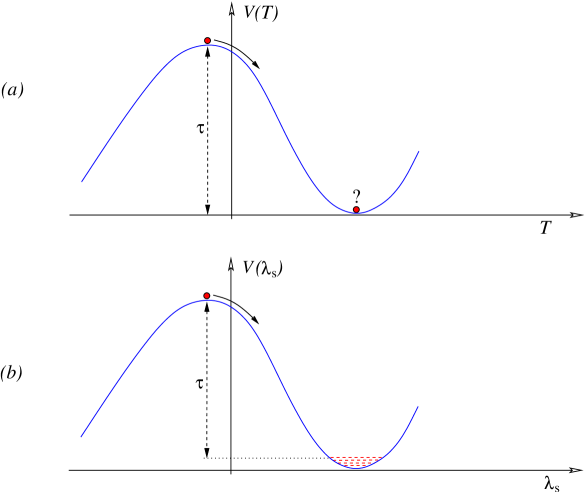
Figure 1: The picture of tachyon condensation: (a) Incomplete in general, due to a lack of a description of the endstate as closed strings, and (b) Complete in the matrix model description, since the sea of eigenvalues at the minimum is a holographic description of the closed string background.

In the double scaled matrix model approach, such diagrams are refined into more precise ones such as that depicted in figure 1(b). The matrix model potential (after double scaling) is the tachyon potential. In the eigenvalue description, at large $N$ the eigenvalues form a droplet (or collection of droplets) in one (or more) of the minima of this potential. The collective excitations of the eigenvalue constituents in these droplets are closed string physics, while the process of moving an eigenvalue out of the collective and up to a extremum of the potential represents the creation of a D–brane, whose tension is given by the energy difference between the sea of collective eigenvalues and the extremum.

Furthermore, it was shown some time ago how to describe, with matrix models, string vacua containing a specific number (say, $\Gamma$) of background D–branes, both for non–perturbatively unstable models[17, 18] and non–perturbatively stable ones[19, 20]. We will be examining these definitions more in this paper. In each set of models, the region of large positive cosmological constant, $\mu$, in each model give identical perturbation theory, and can be identified as having $\Gamma$ background D–branes. The non–perturbatively stable models allow one to continue to a second perturbative region, that of large negative $\mu$, whose interpretation was unclear at the time the models were first presented. Recent work[21] has shown that these non–perturbatively stable models are actually descriptions of the type 0A string theories, and that the large negative $\mu$ perturbative regime has an interpretation in terms of there being $\Gamma$ units of R–R flux. This is an example of an open/closed transition happening as a coupling ($\mu$) in the theory changes. (See refs.[22, 23] for generalizations to the rest of the minimal models for type 0A.)

In this paper we wish to examine in detail some of the key components of these matrix model definitions, and sharpen the understanding of many of the features of the models. A key role is played by the diagonal of the resolvent ${\hat{R}}(z,\lambda_{s})$ of the Schrödinger operator ${\cal H}=-\partial^{2}_{z}+u(z)$, ($\lambda_{s}$ is a spectral parameter) which enters in three logically distinct (but interconnected) ways: (a) It acts as a source for placing D–branes and fluxes into the background, as can be seen from the way it enters the matrix model and the resulting string equations. (b) It acts as a probe of the background, since its first $z$–integral (after a Laplace transform) is the macroscopic loop expectation[24] operator. Its probe character also follows from the fact that its first $z$–integral yields the effective force on a scaled eigenvalue[25]. In order to understand better the physics in the various regimes, we switch on the background, corresponding to including the resolvent in the string equations with strength $\Gamma$, and then we work in each perturbative regime, using the integrated resolvent as a probe to see the effects of the background. We study this probe at disc order in large positive $\mu$ perturbation theory, and to annulus and torus order in large negative $\mu$ perturbation theory, in order to characterize the effects of D–branes and fluxes on the matrix eigenvalues.

(c) The integrated resolvent forms a representation of a twisted boson $\varphi(z)$ in an associated conformal field theory. The entire content of the closed string theory can be expressed in terms of Virasoro constraints[26, 27] —the microscopic loop equations— on the partition function which is realized as wavefunction in a coherent state of the boson. The creation modes of the boson are closed string operator insertions in the string theory. The Virasoro constraints in the presence of $\Gamma$ were worked out in ref.[19] and refined in ref.[20]. It was observed in ref.[20] that the insertion of the D–brane (or flux) background in this language corresponds to just acting with a vertex operator of the twisted boson, $V_{\Gamma}=:\exp(-\Gamma\varphi(\sigma)/2):$ The parameter $\sigma$ corresponds to the boundary cosmological constant.

This latter observation is particularly interesting since it makes extremely explicit (if it were not manifestly so already) the fact that in a fully non–perturbative framework, such as this one, structures that we interpret as open strings in some perturbative regime can be introduced in entirely closed string terms, built out of a specific combination (derived in refs.[28, 20]) of closed string operators . Here we see it succinctly in terms of the vertex operator. This is of course one of the biggest lessons to be taken away from all of this: Open/closed transitions and strong/weak coupling dualities exist because the physics can be specified independently of the perturbation theory (this is also the central lesson of M–theory). When we can get a handle on the right variables whose definition is not rooted in the world–sheet expansions, we can describe the physics in a number of ways, involving open or closed strings.

This also leads one to wonder whether the twisted boson framework should be taken as an equivalent starting point for discussion of the non–critical string theory in various backgrounds. Is there a sense in which it is another (holographic) dual of the theory, or does it rise above that, being the parent theory within which holography and duality become manifest? This would go beyond the recent interesting statements in the literature[31, 32, 33] that the complex curve described by the analytically continued effective potential is simply an alternative target space. Instead, it would suggest that the twisted boson should be given dynamical meaning. Specific solutions for the wavefunctions correspond to certain non–critical string backgrounds we already know, and so we should expect that the dynamics of $\varphi$ can give us more insight into non–perturbative dynamics of string vacua, including perhaps time dependence, if we can find analogous structures in higher dimensional string theories.

There is a fair amount of review material in this paper for which we make no apology. It sets up the language and conventions, and reminds the reader of older (and often highly relevant) literature. The following outline will help the well–informed reader avoid the parts they wish to: In section 2, we recall the string equations for the bosonic and type 0A systems, noting that the former are perturbatively equivalent to the latter in the large positive cosmological constant regime. Section 3 is a detailed review of the double scaled matrix model origins of the bosonic string equations, while section 4 reviews the details of how to extract the effective (tachyon) potential for eigenvalues in the scaling limit. The non–perturbative effects of D–branes (instantons) are recalled. Their tensions are computed from the effective potentials for scaled eigenvalues, and are known from explicit computations (at least for the unitary members of the $(2,2k-1)$ series[12]) to match the tensions of the D–brane of the continuum theory. The interpretation in terms of D–brane world–volume theory and tachyon potentials is discussed in detail there. Sections 5, 6, and 7 review and complete the derivation of aspects of the doubled scaled matrix model origins of the type 0A string equations, explains the connection to the bosonic models, and discusses the differences in non–perturbative effects. This includes a reminder of the role of the two seas of eigenvalues in stabilizing the non–perturbative physics. Section 8 turns to backgrounds with non–trivial open string or R–R flux. The central object in this section is the resolvent, which plays two connected roles here. The first is as a probe of the matrix model in the language of macroscopic loops, or as the effective force on a scaled eigenvalue. We re–derive the effective (tachyon) potential of section 4 from this point of view, now including terms higher order in perturbation theory. The second role is as a source in the string equations which inserts a number of D–branes, or units of flux, into the background. This section has both of these roles working in tandem, since we study the loop operator (eigenvalue dynamics) in the presence of the non–trivial backgrounds. So after a brief review of the properties of the string equations for these situations, we remind the reader of the properties of the scaled loop operator in these theories, and explain the systematics of developing the results for the operator perturbatively, using the string equations together with the Gel’fand–Dikii equation. We derive compact expressions for the loop operator and hence the eigenvalue distributions and effective potentials to disc order (and to annulus and torus order), and analyze the results. In section 9 we remark upon the fluidity of the formalism in its treatment of the closed string and open string sectors. We see that the open string (or flux) backgrounds can be implemented in terms of a specific preparation of closed string operators. This is made much more transparent —and suggestive— in an associated conformal field theory language, which organizes everything. We remind the reader of the formalism[26, 27] of the ₂ twisted boson, and of how the entire content of the string theory is expressed as Virasoro constraints on the partition function. This partition function is realized in the twisted boson framework as a coherent state. We then discuss how[20] the open string or flux background is simply realized by placing a vertex operator into the coherent state background. This shows the remarkable transparency of the formalism with regards working with open or closed string backgrounds.

2 The String Equations

Consider the following equations:

$${\cal R}=2\nu\Gamma{\hat{R}}(z,\sigma)\ ,$$ (1)

and

$$(u-\sigma){\cal R}^{2}-\frac{1}{2}{\cal R}{\cal R}^{{}^{\prime\prime}}+\frac{1}{4}({\cal R}^{{}^{\prime}})^{2}=\nu^{2}\Gamma^{2}\ .$$ (2)

Here $u(z)$ is a real function of the real variable $z$, a prime denotes $\nu\partial/\partial z$, where $\nu$ is a constant, and $\sigma$ and $\Gamma$ are parameters we shall discuss further shortly. We define the quantity:

$${\cal R}=\sum_{k=0}^{\infty}\left(k+\frac{1}{2}\right)R_{k}\ ,$$ (3)

where the $R_{k}$ ($k=0,\ldots$) are polynomials in $u(z)$ and its $z$–derivatives. They are related by a recursion relation:

$$R^{{}^{\prime}}_{k+1}=\frac{1}{4}R^{{}^{\prime\prime\prime}}_{k}-uR^{{}^{\prime}}_{k}-\frac{1}{2}u^{\prime}R_{k}\ ,$$ (4)

and are fixed by the constant $R_{0}$, and the requirement that the rest vanish for vanishing $u$. The first few are:

$$R_{0}=\frac{1}{2}\ ;\quad R_{1}=-\frac{1}{4}u\ ;\quad R_{2}=\frac{1}{16}(3u^{2}-u^{{}^{\prime\prime}})\ .$$ (5)

The $k$th model is chosen by setting all the other $t$s to zero except $t_{0}\equiv z$, and $t_{k}$, the latter being fixed to a numerical value such that ${\cal R}={\cal D}_{k}-z$. The ${\cal D}_{k}$ are normalized such that the coefficient of $u^{k}$ is unity, e.g.:

$${\cal D}_{1}=u\ ,\quad{\cal D}_{2}=u^{2}-\frac{1}{3}u^{{}^{\prime\prime}}\ ,\quad{\cal D}_{3}=u^{3}-uu^{{}^{\prime\prime}}-\frac{1}{2}(u^{{}^{\prime}})^{2}+\frac{1}{10}u^{{}^{\prime\prime\prime\prime}}\ .$$ (6)

The quantity

$${\hat{R}}(z,\lambda)=<z|\frac{1}{({\cal H}-\lambda)}|z>\ ,\quad{\rm where}\quad{\cal H}=-\nu^{2}\frac{\partial^{2}}{\partial z^{2}}+u(z)\ ,$$ (7)

is the diagonal of the resolvent of the Hamiltonian ${\cal H}$ and it satisfies the Gel’fand–Dikii equation[35, 36, 37]:

$$4(u-\lambda){\hat{R}}^{2}-2{\hat{R}}{\hat{R}}^{{}^{\prime\prime}}+({\hat{R}}^{{}^{\prime}})^{2}=1\ .$$ (8)

The function $u$ defines the partition function $Z=\exp(-F)$ of a string theory via:

$$u(z)=\nu^{2}\frac{\partial^{2}F}{\partial\mu^{2}}\Biggl{|}_{\mu=z}\ ,$$ (9)

where $\mu$ is the coefficient of the lowest dimension operator in the world–sheet theory. It is the world–sheet cosmological constant in the case $k=2$ for the bosonic string (in which case we take equation (1)) and $k=1$ for the type 0A string, in which case we take equation (2)). For the case $k=1$ for the bosonic string, $\mu$ couples to a boundary operator measuring lengths.

The equations (1) and (2) have exactly the same physics for large $z$ (equivalent to $\mu$; we will sometimes use the two interchangeably), which corresponds to a perturbative regime. Let us set $\Gamma=0$ and $\sigma=0$ for now. For example, for $k=2$, we have for the free energy (discarding non–universal terms):

$$F=\frac{4}{15}g_{s}^{-2}+\frac{1}{24}\log\mu-\frac{7}{1440}g_{s}^{2}+\cdots\ ,$$ (10)

where the dimensionless parameter $g_{s}={\nu}{\mu^{-5/4}}$ is the closed string coupling. We see the expansion in terms of closed string worldsheets of topology $\chi=2-2h$ ($h$ is the number of handles), each coming with factor $g_{s}^{-\chi}$. The dependence on the sphere displays bosonic KPZ scaling $F(\mu)\sim\mu^{2-\gamma_{str}}$ for the critical exponent (string susceptibility) $\gamma_{\rm str}=-1/k$, and $k=2$ here. For $k=1$, $Z\sim\mu^{3}$, which should be discarded with other non–universal physics, and so this theory has no contribution from any closed string world–sheets. It is a topological theory, as we will recall below. The closed string coupling for this $k=2$ case is $g_{s}=\nu\mu^{-3/2}$. For general $k$, it is:

$$g_{s}=\frac{\nu}{\mu^{1+\frac{1}{2k}}}\ ,$$ (11)

which fits with the fact that

$$u(z)=z^{\frac{1}{k}}+\cdots$$ (12)

and hence:

$$F\simeq\frac{\mu^{\frac{1}{k}+2}}{\nu^{2}}\ .$$ (13)

Non–perturbatively, the situations for each equation, and hence the models they describe, are different. For the case of equation (1), there is a well–known instability[1, 2, 3]. The physics is non–perturbatively problematic for even $k$, there being no sensible real solutions for $u(z)$ which match onto the large $z$ perturbation theory just discussed. This fits with the fact that the model is rendered unstable through a decay channel mediated by instanton effects[25, 38] which we now think of as the nucleation of D–branes.

Let us turn to equation (2), starting again with $\sigma$ and $\Gamma$ set to zero. This equation enjoys better non–perturbative properties than the original string equation (1), (see refs.[39, 40, 41, 19, 42, 43]) while sharing the same perturbative physics for large positive $z$, as follows from the fact that ${\cal R}=0$ is also a solution of this equation, and that for large $|z|$, the leading order equation is $u(u^{k}-z)=0$. So the behaviour $u=z^{\frac{1}{k}}+\ldots$ can be chosen for large positive $z$, and the perturbative expansion is exactly the same as that given in equation (10).

For large negative $z$, however, we can choose a completely different behaviour for solutions of equation (2) from that available for equation (1). We can choose the asymptotic $u=0$ in that regime, having the physics on the sphere vanish for all $k$. The next non–vanishing order is of a universal form for all $k$, and is:

$$u(z)=-\frac{1}{4}\frac{\nu^{2}}{z^{2}}+\cdots\ ,$$ (14)

yielding a universal torus contribution for all models. The full solutions of the equation with these asymptotics for large $\pm z$, for all $k$, are believed to be unique and pole–free supplying a fully consistent non–perturbative physical string theory. See for example the bottom curves of the families depicted in figure 2(a) and (b).

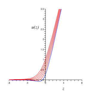
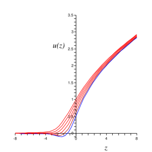
Figure 2: Numerical solutions to equation (2) for $u(z)$: (a) The case $k=1$, and (b) the case $k=2$, for a range of values of the parameter $\Gamma$, with $\sigma=0$. The very bottom curve in each case is the case of $\Gamma=0$. The solutions all asymptote to $u=z^{1/k}$ for large positive $z$ and $u=0$ for large negative $z$.

The cases of $k=1,2$ and 3 have been studied extensively, and (at least) $k=1$ is known to exist uniquely (since it maps[44, 45] to the case of the simplest Unitary matrix model critical point[46, 47] which defines unique physics[48, 49]) and this at least implies a unique family for all $k$ connected by KdV flows[42].

These solutions were proposed as non–perturbative completions of the sick bosonic string models a while ago[39, 40, 41, 19, 42, 43]. That statement has now been refined by recent work[21]: The models have an interpretation as type 0A models. This is consistent with a number of facts, among which is the fact[21] that the spectrum of operators of the Liouville dressed $(2,2k-1)$ conformal minimal models match exactly those of the super–Liouville dressed $(2,4k)$ superconformal minimal models.

3 Matrix Models and Double Scaling 1: Bosonic Strings

Both sets of models can be derived from one–matrix models in the double scaling limit and we can choose Hermitian matrices if we so wish. Equation (1) for $\Gamma=0$ arose for Hermitian matrix models, which can be written in the form:

$${\cal Z}=\int dM\exp\left\{-\frac{N}{\gamma}{\rm{\rm Tr}}\left(V(M)\right)\right\}\ ,$$ (15)

where $M$ is an $N{\times}N$ Hermitian matrix, and the coefficients of the polynomial potential $V(M)$ and the parameter $\gamma$ are tuned to critical values as $N\to\infty$. Recall that the Feynmann diagrams of the matrix model are interpreted as dual to discretisations of the string worldsheets, organized in a genus expansion for large $N$. The path integral is then to be thought of as a particular regularization which enumerates the sum over surfaces. The typical size of a cell in the discretization is set by a parameter we shall call $\delta$. The critical potentials are those which pick out surfaces with diverging area, so that in the continuum limit $\delta=0$ these give finite area contributions to the path integral.

The typical method of study[50] is to diagonalize $M$ using a unitary matrix $U$ into the form $M=U\Lambda U^{\dagger}$, where $\Lambda={\rm diag}\left\{\lambda_{1},\lambda_{2},\ldots,\lambda_{N}\right\}$. There is a Jacobian for this change of variables, which is the square of the Van der Monde determinant $\prod_{i<j}(\lambda_{i}-\lambda_{j})$, and the resulting model is (after dividing by a normalization factor ${\rm Vol}(U(N))$):

$${\cal Z}=\int\prod_{i}d\lambda_{i}\prod_{i\neq j}(\lambda_{i}-\lambda_{j})^{2}\exp\left\{-\frac{N}{\gamma}\sum_{i=1}^{N}V(\lambda_{i})\right\}\ ,$$ (16)

An efficient way of working[51] is to use polynomials $P_{n}(\lambda)\sim\lambda^{n}+\cdots$ which are orthogonal with respect to the measure $d\mu(\lambda)=d\lambda e^{-N/\gamma V(\lambda)}$,

$$\int P_{n}(\lambda)P_{m}(\lambda)d\mu(\lambda)=h_{n}\delta_{nm}\ .$$ (17)

The polynomial $\lambda P_{n}(\lambda)$ must be equal to $P_{n+1}$ plus a correction, which for even potentials (on which we will focus here) is simply:

$$\lambda P_{n}(\lambda)=P_{n+1}(\lambda)+R_{n}P_{n-1}(\lambda)\ ,$$ (18)

where we have defined the coefficient $R_{n}$. Using the orthogonality condition it is given in terms of the $h_{n}$s as $R_{n+1}=h_{n+1}/h_{n}$.

After a little more work, one can write the vacuum energy of the model as[51]:

$$F=-\sum_{n=1}^{N}(N-n)\log R_{n}+\cdots\ ,$$ (19)

where the ellipsis denote parts which are non–universal, and the entire problem is one of determining the $R_{n}$s.

The content of the matrix model can be extracted from the relation:

$$\int d\mu(\lambda)P_{n-1}(\lambda)\frac{d}{d\lambda}P_{n}(\lambda)=nh_{n}\ ,$$ (20)

which amounts, after integrating by parts, to a compact master equation:

$$\sqrt{R_{n}}<n-1|V^{{}^{\prime}}({\hat{\lambda}})|n>=\frac{\gamma n}{N}\ ,$$ (21)

where we have used a bra–ket representation of the orthogonal polynomials and the integration over product pairs of them with respect to the measure. Functions integrated with respect to the measure become operator valued in this representation:

$$|n>=\frac{P_{n}}{\sqrt{h_{n}}}\ ,\quad{\hat{n}}|n>=n\ ,\quad{\cal A}|n>=|n-1>\ ,\quad{\cal A}^{\dagger}|n>=|n+1>$$

$$<m|n>=\delta_{mn}\ ,\quad{\cal A}R_{\hat{n}}=R_{{\hat{n}}+1}{\cal A}\ ,\quad{\cal A}^{\dagger}R_{\hat{n}}=R_{{\hat{n}}-1}{\cal A}^{\dagger}\ .$$ (22)

The recursion relation (18) define

$${\hat{\lambda}}=\sqrt{R_{\hat{n}}}{\cal A}^{\dagger}+{\cal A}\sqrt{R_{\hat{n}}}\ ,$$ (23)

which allows a rewriting of the master equation in the equivalent form:

$$<n|{\hat{\lambda}}V^{\prime}({\hat{\lambda}})|n>=\frac{\gamma}{N}(2n+1)\ ,$$ (24)

which will be useful later on. It is convenient to write our master equation (21) a touch more compactly as:

$$<n|{\cal A}^{\dagger}V^{{}^{\prime}}({\hat{\phi}})|n>=\frac{\gamma n}{N}\ ,$$ (25)

where

$${\hat{\phi}}={\cal A}^{\dagger}+{\cal A}R_{\hat{n}}\ ,\quad\sqrt{h_{\hat{n}}}{\hat{\phi}}={\hat{\lambda}}\sqrt{h_{\hat{n}}}\ .$$ (26)

The master equation is now actually a recursion relation for the $R_{n}$, as can be seen by expanding for a given potential $V(\lambda)$. The higher the order of $V(\lambda)$, the more terms there are in the recursion relation.

The continuum limit is then easily approached in these variables. At large $N$ we pass to a continuum limit in eigenvalues space as well, and write $x=n/N$, $R(x)=R(n/N)$, $\epsilon=1/N$. The master equation is:

$$<x|{\cal A}^{\dagger}V^{\prime}({\hat{\phi}})|x>=\gamma x\ ,$$ (27)

and the free energy is:

$$F=-N^{2}\int_{0}^{1}dx(1-x)\log R(x)\ .$$ (28)

Focusing on the sphere contribution means dropping terms subleading in $N$ and so the difference equations become polynomial relations in $R(x)$:

$$1-\gamma x=P(R(x))\ .$$ (29)

The required divergent behaviour of the free energy $F\sim(\gamma_{c}-\gamma)^{2-1/k}$ occurs when the polynomial in $R(x)$ acquires $k$ multiple roots: $P(R)=(R-R_{c})^{k}$. This amounts to choosing particular values of the couplings in the potential[52] and also tuning $\gamma$ to a critical value $\gamma_{c}$. The critical value of $R(x)$ at this point can be chosen to be equal to 2, and in the neighbourhood $\gamma x=1$, without loss of generality. We can choose a potential of degree $2k$ to get the above behaviour, and a convenient basis is[53]:

$$V_{1}(\phi) = \frac{1}{4}\phi^{2}\ ;$$

$$V_{2}(\phi) = \frac{1}{2}\phi^{2}-\frac{1}{48}\phi^{4}\ ;$$

$$\vdots = \vdots$$

$$V_{k}(\phi) = \sum_{i=1}^{k}(-1)^{i-1}\frac{k!(i-1)!}{2^{i}(k-i)!(2i)!}\phi^{2i}\ .$$ (30)

Finite physics is extracted by allowing $R(x)$ and $\gamma x$ to approach their critical values at the right rate as $\delta\to 0$. The quantity $\epsilon=1/N$ must also be scaled with $\delta$ so as to approach zero at the correct rate:

$$\gamma=1-\frac{\mu}{4}\delta^{2k}\ ;$$

$$\gamma x=1-\frac{z}{4}\delta^{2k}\ ;$$

$$R(x)=2-u(z)\delta^{2}\ ;$$

$$\epsilon=\frac{\nu}{4\sqrt{2}}\delta^{2k+1}\ .$$ (31)

(Numerical prefactors of the scaled quantities $\mu,z,u(z)$ and $\nu$ are chosen for convenience.) To go beyond the sphere one simply keeps the $1/N$ contributions in the master difference equation, and in the large $N$ limit it becomes a differential equation. Inserting the scalings into the master equation and expanding about $\delta=0$ gives for the first non–vanishing terms, a differential equation of order $2k-2$ at order $\delta^{2k}$. So in taking the limit $\delta\to 0$, this is the surviving physics and it is in fact equation (1), with $\Gamma=0$, $\sigma=0$ and all $t$s set to zero except $t_{0}\sim z$ and $t_{k}$.

By introducing dimensionful coefficients $t_{k}$ for each potential, we can consider the general model. From the point of view of the $k$th theory, the other $t_{k}$s represent coupling to closed string operators ${\cal O}_{k}$. It is well known that the insertion of each operator can be expressed in terms of the KdV flows[54, 24]:

$$\frac{\partial u}{\partial t_{k}}=R^{{}^{\prime}}_{k+1}\ .$$ (32)

The operator ${\cal O}_{0}$ couples to $t_{0}$, which is in fact $-4z$, the cosmological constant (in the unitary model). So ${\cal O}_{0}$ is often referred to as the puncture operator, which yields the area of a surface by fixing a point which is then integrated over in the path integral. The function $u$ itself can be thought of as the two point function of the puncture operator.

4 Effective Tachyon Potentials and D–Branes: Bosonic Strings

It is also important to keep in mind the eigenvalue picture. The eigenvalues take values on the real line. The Van der Monde determinant acts as a repulsive potential, driving them apart, but they are confined by the potential $V(\lambda)$ to form a droplet of finite size at large $N$. At large $N$, at the spherical level, one can solve for a density $\rho(\lambda)$ of eigenvalues on the line. A relation between the orthogonal polynomial quantity $R(x)$ and the eigenvalue density $\rho(\lambda)$ can be derived at sphere level[51]:

$$\rho(\lambda)=\int_{0}^{1}\frac{dx}{\pi}\frac{\theta(4R(x)-\lambda^{2})}{\sqrt{4R(x)-\lambda^{2}}}\ .$$ (33)

From this expression, it is clear that the ends of the eigenvalue density are located at $\lambda_{c}=\pm 2\sqrt{R_{c}}$. Recalling that the neighbourhood of $x=1$ is where the interesting physics comes from, we must pick one of them to which to scale our physics:

$$\lambda=2\sqrt{2}-\frac{\lambda_{s}}{\sqrt{2}}\delta^{2}\ .$$ (34)

This, together with the scalings (31) gives an expression for the scaled density:

$$\rho(\lambda_{s})=-\frac{\delta^{2k-1}}{16\pi}\int^{\mu}\frac{dz}{\sqrt{\lambda_{s}-u(z)}}=\frac{\delta^{2k-1}}{16\pi}\int_{\mu^{1/k}}^{\lambda_{s}}\frac{ku^{k-1}du}{\sqrt{\lambda_{s}-u(z)}}\ ,$$ (35)

where we have used that $u(z)=z^{1/k}$ on the sphere. Explicit computation of the integral yields[40]:

$$\rho_{(k)}(\lambda_{s})=\frac{k!\delta^{2k-1}}{16\pi}\sum_{n=1}^{k}\frac{2^{n}}{(k-n)!(2n-1)!!}(\lambda_{s}-\mu^{\frac{1}{k}})^{n-\frac{1}{2}}\mu^{1-\frac{n}{k}}+\cdots\ ,$$ (36)

where we remind the reader again that this is valid only at the sphere level.

Crucially, note that since there is a common factor $(\lambda_{s}-\mu^{1/k})^{\frac{1}{2}}$, the eigenvalue density vanishes at $\lambda_{s}=\mu^{1/k}$ as $\lambda^{\frac{1}{2}}$. There are $k-1$ more zeros which are located away from this endpoint. For $k$ even there is another zero at $\lambda<0$ and $k-2$ zeros off the real line in pairs. For $k$ odd, there are no other zeros on the real line, and only pairs of zeros off the real line. In general, $\rho(\lambda)$ is real on the part of the real line where the eigenvalue are located but its complex parts are meaningful also, as we shall see.

A most important quantity is the effective potential that an individual eigenvalue sees[25]. It is minus the change in energy as the eigenvalue moves from $\lambda_{i}$ to $\lambda_{f}$, and is given by the expression:

$$V_{\rm eff}(\lambda)=N\int_{\lambda_{f}}^{\lambda_{i}}d\lambda(V^{{}^{\prime}}(\lambda)-2F(\lambda))=2\pi N{\rm Im}\int_{\lambda_{f}}^{\lambda_{i}}d\lambda\rho(\lambda)\ ,$$ (37)

where

$$F(\lambda)=\int\frac{\rho(\xi)d\xi}{\lambda-\xi}$$ (38)

is the matrix model resolvent. So starting with the eigenvalue on the cut and moving it to anywhere else on the cut costs no energy, since $\rho(\lambda)$ is real there. In scaled variables the effective potential becomes[40]:

$$V_{{\rm eff}}^{(k)}(\lambda_{s})=\frac{2\pi}{\nu\delta^{2k+1}}\int_{\lambda_{s}}^{\mu^{1/k}}\delta^{2}\rho(\lambda^{{}^{\prime}}_{s})d\lambda^{{}^{\prime}}_{s}\ ,\qquad\lambda_{s}<\mu^{\frac{1}{k}}\ .$$ (39)

Inserting our previous expression for the density gives[40]:

$$V_{{\rm eff}}^{(k)}(\lambda_{s})=\frac{1}{\nu}\sum_{n=1}^{k}\frac{k!(-2)^{n+1}}{(k-n)!(2n+1)!!}(\mu^{\frac{1}{k}}-\lambda_{s})^{n+\frac{1}{2}}\mu^{1-\frac{n}{k}}+\cdots\ ,\qquad\lambda_{s}<\mu^{\frac{1}{k}}\ .$$ (40)

Looking at the first two cases explicitly is illustrative:

$$V_{\rm eff}^{(1)}(\lambda_{s}) = \frac{4}{3\nu}(\mu-\lambda_{s})^{\frac{3}{2}}+\cdots\ ,\quad\lambda_{s}<\mu\ ,$$

$$V_{\rm eff}^{(2)}(\lambda_{s}) = \frac{8}{3\nu}(\mu^{\frac{1}{2}}-\lambda_{s})^{\frac{3}{2}}\mu^{\frac{1}{2}}-\frac{16}{15\nu}(\mu^{\frac{1}{2}}-\lambda_{s})^{\frac{5}{2}}+\cdots\ ,\quad\lambda_{s}<\mu\ .$$ (41)

Their behaviours are sketched in figure 3.

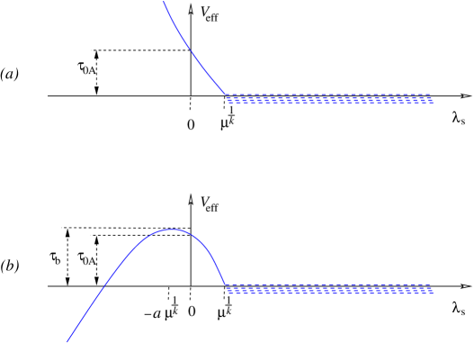
Figure 3: The effective potential for one eigenvalue in the scaling limit, computed at string theory tree level. This is equivalent to the tachyon potential on the world–volume theory of the D–branes. The sea of eigenvalues is to the right in each sketch, on which $V_{\rm eff}=0$. The collective physics of the sea describes closed string physics. A D–brane is described by a single eigenvalue separated from the sea, and its decay by rolling back of the eigenvalue into the sea. The energy released in decay sets the tension of the D–brane. Shown is the difference between the D–brane tension in the bosonic ($\tau_{\rm b}$) and that of the type 0A theory ($\tau_{\rm 0A}$) for the cases of (a) $k$ odd and (b) $k$ even. In the 0A case, the potential stops at $\lambda_{\rm s}=0$, setting a lower value for the D–brane tension.

The key point is that there is a turning point of the effective potential at every zero of the eigenvalue density. In particular we see that the even $k$ cases have a maximum of the potential at one point on the real axis at $\lambda_{s}<0$. The odd $k$ cases have an effective potential which forever rises to the left. To the right in figure 3 is the sea of the other eigenvalues, starting at $\lambda_{s}=\mu^{\frac{1}{k}}$ and going off to infinity.

In the spirit of ref.[4], the interpretation of this physics in the continuum string theory is as follows. The matrix model, once double–scaled, is the theory on the world–volume of $N$ unstable D–branes in the continuum string theory. This model is constituted by a matrix–valued tachyonic field made by open strings interconnecting the $N$ D–branes. The computation above is a precise determination of the potential of the tachyon field at sphere level in string perturbation theory. We have a precise model in which we see holography at work, together with a model of tachyon condensation. To the right is the sea of $N$ eigenvalues. The collective dynamics of these represents closed string physics: Bosonic non–critical string theory given by Liouville theory coupled to the $(2k-1,2)$ conformal minimal models. For this model, the full family of critical potentials given in equation (30) forms a basis for the closed string deformations. They can be added to the model with coefficients $t_{k}$ and are dual to inserting closed string operators ${\cal O}_{k}$ to the model. These are the Liouville dressed conformal field theory operators. As is well known[54, 24], this family of operators is organized by the KdV flows of equation (32).

There is more, however[4]. A single eigenvalue can be removed from the sea and moved up the potential. This describes the creation of a D–brane of the continuum string theory, and it can decay back to closed strings by rolling back down the potential to rejoin the sea. Consistent with this identification is the observation of the behaviour of the tension of the D–brane. The tension of the D–brane should be the energy needed to move up the potential to a definite position which goes like: $\lambda_{s}\sim c\mu^{\frac{1}{k}}$, where $c$ is a constant. Upon examination of the potential $V_{\rm eff}^{(k)}$ it can be seen to behave as:

$$\tau\sim V_{\rm eff}^{(k)}(c\mu^{\frac{1}{k}})\sim C\frac{\mu^{1+\frac{1}{2k}}}{\nu}=\frac{C}{g_{s}}\ ,$$ (42)

where $C$ is a constant. This is the correct behaviour for a D–brane’s tension.

For $k$ even, there is a special class of D–branes formed by placing an eigenvalue at the maximum of the potential, located at $\lambda_{s}=\lambda_{c}$. This is a D–brane which dominates the non–perturbative contributions to the closed string physics, an observation going back to ref.[55]. Its tension is:

$$\tau^{(k)}_{\rm b}\sim V_{\rm eff}^{(k)}(\lambda_{c})\ ,\qquad{\rm for}\,\,\,k\quad{\rm even}\ .$$ (43)

For example, the case $k=2$, since the potential has a maximum at $\lambda_{c}=-\frac{1}{2}\mu^{\frac{1}{2}}$, we get[55, 56]:

$$\tau^{(2)}_{\rm b}=V_{\rm eff}^{(2)}\left(-\frac{1}{2}\mu^{\frac{1}{2}}\right)=\frac{4\sqrt{6}}{5}\frac{1}{g_{s}}\ ,\quad g_{s}=\frac{\nu}{\mu^{\frac{5}{4}}}\ .$$ (44)

This actually shows up as the action of the D–instanton effects arising by studying the leading contribution to effects invisible in perturbation theory. Taking a solution $u_{0}(z)$ of the equation:

$$-\frac{1}{3}u_{0}^{{}^{\prime\prime}}+u_{0}^{2}=z\ ,$$ (45)

one can consider a perturbation $\epsilon(z)$, and study another solution $u(z)=u_{0}(z)+\epsilon(z)$. Assuming that $\epsilon$ is small, and of the form $\epsilon=\exp(-f)$, where $f>>f^{\prime}>>f^{\prime\prime}$, etc., the result[55] is for $u_{0}=z^{1/2}$:

$$\epsilon=e^{-\frac{4\sqrt{6}}{5}\frac{1}{g_{s}}}\ .$$ (46)

This D–brane, (and its analogue for all $k$ even) as can be seen from the effective potential, destabilizes the theory for $k$ even, since the eigenvalue can roll off to infinity to the left of the figure 3(b). This process dooms the $k$ even models[25, 38]. Note that we should be careful not to confuse the instanton effects derived from analyzing perturbation theory and those of the real destabilising instanton see in the effective potential. They match in this case, but existence of one does not imply the other, as we shall recall for the type 0A models[40].

5 Matrix Models and Double Scaling II: Type 0A Strings

The equation (2) also arises from matrix models in a very natural manner. It first appeared in the context of complex matrix models[39], but can be derived from Hermitian matrix models as well. The key point is that the complex matrix models can be formulated as usual in terms of eigenvalues, $\lambda$, of the matrix $M^{\dagger}M$, which are positive. Therefore the problem naturally places a boundary or “wall” at $\lambda=0$. The large positive $z$ regime corresponds to the distribution pulling way from the wall, and so the system resembles the eigenvalue distributions of the one–cut Hermitian matrix models and yields the same perturbation theory. The large negative $z$ limit is very different however, as the distribution pushes up against the wall, and gives very different physics which we will discuss at length shortly. Another way to look at it is in the space ${\tilde{\lambda}}$ where ${\tilde{\lambda}}^{2}=\lambda$. This is the natural eigenvalue space of one matrix. Then we see that there are two identical eigenvalue distributions, one on ${\tilde{\lambda}}\in[0,+\infty)$ and the other (a mirror image) on ${\tilde{\lambda}}\in(-\infty,0]$. See figure 4(a). These distributions either pull apart ($z\to+\infty$) or push together $z\to-\infty$.

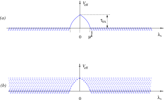
Figure 4: (a) Sketch of the effective potential on the covering space for arbitrary $k$. (b) As $\mu$ decreases, the eigenvalues fill up closer to the top of the potential, decreasing the tension of the available D–brane, until at $\mu=0$, there is no brane available.

For completeness, it is worth recalling how to derive the string equation. We choose the case of an Hermitian matrix model, and we simply introduce a boundary in the eigenvalue space. One can define polynomials orthogonal to the measure $d\mu(\lambda)=d\lambda e^{-N/\gamma V(\lambda)}$ on the interval $[-\Sigma,\Sigma]$, modifying equation (17):

$$\int_{-\Sigma}^{\Sigma}P_{n}(\lambda)P_{m}(\lambda)d\mu(\lambda)=h_{n}\delta_{nm}\ .$$ (47)

The non–trivial (for even potential $V(\lambda)$) relations generalizing equation (21) (or more specifically, the form given in equation (24)) are[57]:

$$<n-1|V^{{}^{\prime}}({\hat{\lambda}})|n> = \frac{\gamma n}{N\sqrt{R_{n}}}+\frac{2\gamma}{N}\frac{P_{n}(\Sigma)P_{n-1}(\Sigma)}{\sqrt{h_{n}h_{n-1}}}e^{-\frac{N}{\gamma}V(\Sigma)}\ ,$$

$$<n|{\hat{\lambda}}V^{{}^{\prime}}({\hat{\lambda}})|n> = \frac{\gamma}{N}\left((2n+1)-2\Sigma\frac{P_{n}(\Sigma)^{2}}{h_{n}}e^{-\frac{N}{\gamma}V(\Sigma)}\right)\ ,$$ (48)

where we have used that, for even potentials, $P_{n}(-\lambda)=(-1)^{n}P_{n}(\lambda)$. We can eliminate the boundary terms to give:

$$\frac{1}{4}\left(\frac{\gamma(2n+1)}{N}-<n|{\hat{\lambda}}V^{{}^{\prime}}({\hat{\lambda}})|n>\right)\left(\frac{\gamma(2n-1)}{N}-<n-1|{\hat{\lambda}}V^{{}^{\prime}}({\hat{\lambda}})|n-1>\right)$$

$$=\Sigma\left(\frac{\gamma n}{N\sqrt{R_{n}}}-<n-1|V^{{}^{\prime}}({\hat{\lambda}})|n>\right)^{2}\ .$$ (49)

Note that

$$<n|{\hat{\lambda}}V^{{}^{\prime}}({\hat{\lambda}})|n>=\sqrt{R_{n}}<n|{\cal A}^{\dagger}V^{{}^{\prime}}({\hat{\lambda}})|n>+\sqrt{R_{n+1}}<n|{\cal A}V^{{}^{\prime}}({\hat{\lambda}})|n>\ ,$$ (50)

and move to the continuum variables as before, defining

$$\Omega(x)=\gamma x-<x-\epsilon|V^{\prime}({\hat{\phi}})|x>\ .$$ (51)

Then the equation becomes:

$$\left[\Omega(x)+\Omega(x+\epsilon)\right]\left[\Omega(x-\epsilon)+\Omega(x)\right]=4\frac{\Sigma}{R(x)}\Omega^{2}(x)\ .$$ (52)

Using the scalings given in equation (31), the critical potentials given in equation (30), and placing the walls at the ends of the critical eigenvalue density at $\Sigma=R_{c}$ we get the string equations (2) in the limit $\delta\to 0$, having appeared at first non–vanishing order $\delta^{4k+2}$.

6 Matrix Models and Double Scaling III: Including Open Strings

In this section, we discuss how the full string equations (1) and (2), with all parameters switched on, arise in the matrix models.

Let’s first turn to non–zero $\sigma$ appearing in equation (2). In fact, $\sigma$ naturally appears in the problem as the scaled position of the wall, which should be a physical parameter as well[57]. In taking the double scaling limit, scaling the position according to $\Sigma=R_{c}(1-\sigma\delta^{2}/2)$, yields the equation (2) with non–zero $\sigma$. Well behaved solutions for non–zero sigma are known to exist, and their behaviour is given numerically in figure 5.

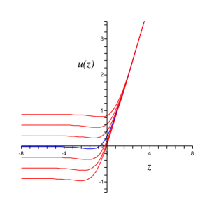
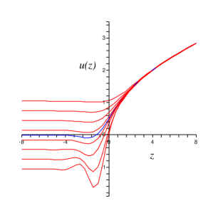
Figure 5: Solutions to equation (2) for $u(z)$, with asymptitics given in figure 2. (a) The case $k=1$, and (b) the case $k=2$, for a range of values of the parameter $\sigma$ with $\Gamma=0$. The middle curve in each case is the case of $\sigma=0$.

Next, let us note that there is an important quantity which arises in the continuum limit of the matrix models which will play an important role here and later. In the bra–ket formalism introduced earlier, the operator ${\hat{\lambda}}$ in equation (26) can be directly formulated as a differential operator[53]. This comes because the shift operators ${\cal A},{\cal A}^{\dagger}$ get represented as derivative operators $\exp\left(\epsilon\partial_{x}\right),\exp\left(-\epsilon\partial_{x}\right)$ acting on functions of $x=n/N$. Recall also that there is a specific scaling for the objects from which ${\hat{\lambda}}$ is made, given in equation (31), so we can expand it and see what its scaling is in the limit $\delta\to 0$ and we find that:

$${\hat{\lambda}}=2\sqrt{R_{c}}+\frac{1}{\sqrt{2}}\left(\nu^{2}\frac{\partial^{2}}{\partial z^{2}}-u(z)\right)\delta^{2}+\cdots={\hat{\lambda}}_{c}-\frac{\cal H}{\sqrt{2}}\delta^{2}+\cdots$$ (53)

The Schrödinger operator ${\cal H}$ plays a crucial and very natural role in what is to come.

The matrix model origin of the string equation (1) with non–zero $\Gamma$ arises by adding a term[17, 18]

$$\Delta V(M)=\frac{\Gamma}{N}{\rm Tr}\log\left(1-s^{2}M^{2}\right)$$ (54)

to the matrix model potential. In the world–sheet dual to the Feynmann diagrams, this corresponds to adding holes of all sizes, by expansion of the logarithm. This new term adds new pieces to the master equation (24):

$$\frac{\Gamma}{N}\left(1-<n|\frac{1}{1-s^{2}{\hat{\lambda}}^{2}}|n>\right)\ .$$ (55)

On the sphere, there is still the critical behaviour where large area surfaces dominate, near $R=R_{c}$, but there is an additional critical point near a critical value of $s$ set by $s_{c}^{-1}=2\sqrt{R_{c}}$. This arises because, e.g., on the sphere, the last term in equation (55) reduces to $-(\Gamma/N)(1-4s^{2}R(x))^{-1/2}$. So the lengths of loops can chosen to diverge if we send $s\to s_{c}$, but give finite length loops as $\delta\to 0$ if we scale at the right rate. Since near the critical point the new terms are:

$$-\frac{\Gamma}{N}\frac{1}{[4(s^{2}_{c}-s^{2})R_{c}+(R_{c}-R)/R_{c}]^{\frac{1}{2}}}\ ,$$ (56)

this rate turns out to be $s^{2}=s^{2}_{c}-\sigma\delta^{2}$. The factor of $1/N$ scaling as $\delta^{2k+1}$ produces the appropriate damping of the divergence and the string equation (1) results (as before) at order $\delta^{2k}$, the resolvent arising from the appearance of ${\cal H}$ in the scaling part of ${\hat{\lambda}}$, appearing at the same order in $\delta$ as $\sigma$ does.

The same procedure can be applied to the master equations (49) arising from placing walls in the system. As happens before, order $\delta^{4k+2}$ is where the non–trivial physics appears, and the lefthand side of the string equation (2) appears at this order, while the right hand side, $\nu^{2}\Gamma^{2}$ appears multiplying $-1$ times the left hand side of the Gel’fand–Dikii equation (8), with $\lambda$ set to $\sigma$. Thus we arrive at equation (2). So this is how the position of the walls and the weight factor of the loops become related in the continuum model. In effect, the argument of the logarithm diverges (so as to give finite length loops in the continuum limit) at the same place in eigenvalue space at which the walls are located.

Another way to see that this must be true is to imagine that equation (2) was true, but for another parameter $\tau$, instead of $\sigma$. How can we fix $\tau$? Taking sums and differences of the equations we see that we have a condition that either $\tau=\sigma$ and the equation (2) follows, or we have ${\cal R}=0$, in which case $\Gamma=0$. This matches what we learned from the matrix model. If we do not scale the parameters so as to make the logarithm diverge precisely at the ends, then it produces no new physics.

7 Effective Tachyon Potentials and D–Branes in Type 0A String Theory

Turning to the issue of instantons arising from analyzing perturbation expansions, we note[40] that there is another instanton contribution to the large positive $z$ perturbation theory. Searching as before for the perturbation $\epsilon=e^{-f}$, we get the same instanton as for the equation (1), and in addition, there is an equation:

$$(u_{0}-\frac{\nu^{2}}{4}(f^{{}^{\prime}})^{2}){\cal R}^{2}=0\ ,$$ (57)

which, upon using $u_{0}=z^{\frac{1}{k}}$, gives instanton:

$$\epsilon\sim e^{-\frac{4k}{2k+1}\frac{1}{g_{s}}}\ .$$ (58)

This instanton can be connected to the physics of the effective potentials we have already studied. See figures 3 and 4(a). For large positive $z$, the results from before will still apply (after a shift of the origin of coordinates to place one of the walls there), modified only by the fact that the eigenvalues must be positive. Looking at the effective potentials, we see that since there is a wall at $\lambda_{s}=0$, the instanton at negative $\lambda_{s}$ previously encountered for $k$ even cannot destabilize the system. There is an instanton for all $k$ at the wall, and its tension is given by $V^{(k)}_{\rm eff}(0)$, which a computation shows is:

$$\tau_{0A}=V_{\rm eff}(\lambda_{s}=0)=\frac{4k}{2k+1}\frac{\mu^{1+\frac{1}{2k}}}{\nu}\ .$$ (59)

This is the same action as the new instanton perturbations of the solutions we saw above. So we see that although the same instanton which destabilised the bosonic theory is present in the analysis, it does not represent an instability[40].

Since the role of $\sigma$ in the matrix model is to move the wall, as we saw in the previous section, it can be seen as an interpolating parameter in some sense, since the limit of large negative $\sigma$ approaches (but never reaches) the physics of the unstable bosonic models[58]. See figure 5(b). Notice for example how as $\sigma$ becomes more negative, for the case $k=2$, the system begins to develop more fluctuations at negative $z$, ultimately heralding the poles that exist on the negative $z$ axis for the Painlevé I equation (equation (1) for $k=2$.). Studies of this sort were presented in ref.[58].

The physical role of $\sigma$ from the point of the continuum string theory is more subtle. It represents a non–perturbative contribution to the coupling of a boundary operator ${\cal O}_{\rm B}$ which measures the length of world–sheet boundaries or loops[58]. It is a boundary cosmological constant and we will examine it in some more detail in the next section. Note that for the models defined by equation (1) with $\Gamma=0$, the boundary length operator for the $k$th model is identified with ${\cal O}_{k-1}$. See ref.[59]. In particular, for $k=1$, the operator is ${\cal O}_{0}$ which couples to $t_{0}\sim z$. For this case, (and for the $k=1$ solution of equation (2) for large positive $z$) it is interesting to note that $\sigma$ can be absorbed into $z$ without changing the universal physics. So we see that $\sigma$ is indeed a natural realization of the boundary cosmological constant, by matching onto the perturbatively identified boundary operator.

Recall that the $k=1$ model has no expansion in terms of closed string world–sheets. The theory’s entire content comes alive when the other operators ${\cal O}_{k}$ are inserted, and their correlation functions at genus $h$ are then seen to be isomorphic to intersection numbers on the moduli space of Riemann surfaces of genus $h$: it is a topological theory. The $k=1$ solution of equation (2) (for large $z$) shares this behavior, but develops new features in the non–perturbative regime. In fact, this is a precise example of a non–perturbative completion of a topological theory, and deserves further study from this perspective. It can be rewritten as the type 0B model in the same background, as identified in ref.[21] using the change of variables of refs.[44, 45].

As we will recall below the partition function of the $k=1$ theory (exactly for equation (1) and at large positive $z$ for equation (2)) only has a topological expansion in the presence of D–branes, giving only world–sheets with boundaries in the expansion.

8 Loops and D–Branes for Bosonic and Type 0A Strings

Now we turn to the physics of non–zero $\Gamma$. A study of equation (2) for non–zero $\Gamma$ shows that large positive $z$ (or $\mu$) perturbation theory has an interpretation as including world–sheet boundaries, and in fact $\Gamma$ counts the number of D–branes in the background, as can be seen by the fact that a factor $\Gamma^{b}$ appears for a surface with the number of boundaries equal to $b$. For example, for $k=2$:

$$F = \frac{4}{15}g_{s}^{-2}+\frac{8\Gamma}{5}g_{s}^{-1}+\frac{(6\Gamma^{2}+1)}{24}\log\mu-\frac{(4\Gamma^{3}+3\Gamma)}{48}g_{s}-\frac{1}{5760}(180\Gamma^{4}+345\Gamma^{2}+28)g_{s}^{2}+\cdots$$ (60)

$$= \sum_{h,b}C_{b,h}g_{s}^{2h-2+b}\Gamma^{b}\ .$$

The equation supplies fully non–perturbative completions of this physics, including the following behaviour at large negative $z$ (or $\mu$):

$$F = -\frac{(4\Gamma^{2}-1)}{4}\log\mu$$

$$+(4\Gamma^{2}-1)(4\Gamma^{2}-9)(4\Gamma^{2}-25)\left\{\frac{1}{960}g_{s}^{4}+\frac{1}{30720}(48\Gamma^{4}-1240\Gamma^{2}+8371)g_{s}^{8}\right\}+\cdots\ ,$$

where the first term is universal to all $k$. At face value, the interpretation in terms of boundaries can be made in this regime as well, but explanation for the number of exactly vanishing orders in perturbation theory (all surfaces with an odd number of boundaries, for example) is needed. Instead, ref.[21] pointed out that in this regime, there are no branes, but instead R–R fluxes, using facts from the continuum type 0 theories and the matrix model. Here, we’ll study the matrix models further and uncover the effective potential beyond tree level in both regimes. Its behaviour in the different regimes clearly give support to this interpretation.

The large positive $z$ perturbation theory of the equation matches perturbation theory obtained from equation (1), which for non–zero $\Gamma$ and $\sigma$ was formulated in refs.[17, 18]. $\Gamma$ appears multiplying the resolvent, which in turn satisfies equation (8). In fact, the most efficient way to construct a perturbative expansion for $u(z)$ is to treat equation (1) as an equation for ${\hat{R}}$ and then substitute it into the resolvent equation, yielding an equation for ${\cal R}$ and hence for $u(z)$. This of course yields the equation (2). Of course, this larger equation allows solutions for $u(z)$ which are not solutions of equation (1). These are the solutions which have the well defined large negative $z$ asymptotics and accompanying pleasant non–perturbative behaviour which we now associate to type 0A. See the families of curves displayed in figure 2.

That the resolvent appears explicitly in the description of D–branes in the backgrounds is interesting because the same object is known to control the behaviour of macroscopic loops in the continuum theory[24]. This is worth recalling in some detail: In the matrix model, it is natural to consider the Wilson loop:

$$W(\ell)=\langle\frac{1}{N}{\rm Tr}e^{\ell M}\rangle\ .$$ (62)

Its Laplace transform is

$$W(\lambda)=\langle\frac{1}{N}{\rm Tr}\frac{1}{\lambda-M}\rangle=\int_{0}^{\infty}d\ell e^{-P\ell}W(\ell)\ .$$ (63)

and in the continuum limit it is:

$$W(\lambda)=\int d\xi\frac{\rho(\xi)}{\lambda-\xi}\ .$$ (64)

The saddle point equation of the matrix model is:

$$\frac{V^{\prime}(\lambda)}{2}={\bf P}\int_{\cal C}d\xi\frac{\rho(\xi)}{\lambda-\xi}\ ,$$ (65)

where $\bf P$ denotes the principal part and the integral is over the support ${\cal C}$ of the density function, $\rho(\lambda)$, of eigenvalues $\lambda$. The density is normalized according to $\int d\lambda\rho(\lambda)=1$. The real part of $W$ is equal to $V^{\prime}/2$ on the support of $\rho(\lambda)$ where its imaginary part is non–zero. This is nicely expressed by the equation (see ref.[60] for a useful presentation):

$${\rm Im}[P(\lambda)]={\rm Im}(V^{\prime}W-W^{2})=(V^{\prime}-2{\rm Re}W){\rm Im}W=0$$ (66)

with solution

$$W(\lambda)=\frac{V^{\prime}(\lambda)}{2}\pm\frac{1}{2}\sqrt{(V^{\prime})^{2}-4P(\lambda)}\ .$$ (67)

where $P(\lambda)$ is fixed by the asymptotic $W(\lambda)\to-1/\lambda$ as $\lambda\to\infty$, given the normalization of the density. By definition, $\rho(\lambda)$ is given by the discontinuity of $W(\lambda)$ on the cut ${\cal C}$.

The connection with the continuum loop operator and the continuum resolvent operator comes from the definition:

$$W(\lambda)=\frac{V^{\prime}}{2}+\delta^{2k-1}w(\lambda_{s})$$ (68)

where, as before, $\lambda_{s}$ is the scaling part of $\lambda$.

Now the marvellous thing[24] is that

$$w(\lambda_{s})=\int\!dz\,{\hat{R}}(z,\lambda_{s})=\int dz<z|\frac{1}{({\cal H}-\lambda_{s})}|z>\ ,$$ (69)

and it is the Laplace transform of the continuum loop

$$w(\ell)=\int dz<z|e^{-\ell{\cal H}}|z>\ ;\qquad w(\lambda_{s})=\int_{0}^{\infty}d\ell e^{-\lambda_{s}\ell}w(\ell)$$ (70)

The Schrödinger operator ${\cal H}$ arose earlier in equation (53). Loops correspond to expectation values of traces of powers of matrices ${\rm Tr}{M^{p}}$ where $p=\frac{\ell}{\delta}$. This corresponds to cutting a $p$–sided hole in the dual picture of discretized worldsheets. We hold $\ell$ fixed by sending $p$ to infinity as we send $\delta\to 0$. In the bra–ket formalism this amounts to computing the Laplace transform of the resolvent ${\hat{R}}(z,\lambda_{s})$, and we integrate over $z$ (up to some reference value, $\mu$ although we will still use $z$ for a lot of what follows) to get the expectation value $w(\ell)\sim\int dz<z|{\hat{\lambda}}^{\frac{\ell}{\delta}}|z>$, which gives the first expression in equations (70).

Notice that $w(\lambda_{s})$ is also (up to a factor $\nu/2$) the first $\lambda_{s}$–derivative of the effective potential $V_{\rm eff}(\lambda_{s})$, and this gives an efficient way of deriving the effective potentials for the system to arbitrary order in perturbation theory, by use of the string equations in combination with the resolvent equation. In particular, the procedure is to solve either string equation for $u(z)$ to desired order in perturbation theory, keeping some non–zero value of $\sigma$. This is now to be treated as a potential for the Hamiltonian ${\cal H}$, and one can solve for its resolvent ${\hat{R}}(z,\lambda_{s})$ to that order in perturbation theory by using equation (8). The next step is to integrate once with respect to $z$ to get the loop operator $w(\lambda_{s})$, and one can integrate once with respect to $\lambda_{s}$ to get the effective potential $V_{\rm eff}$:

$$V_{\rm eff}=\frac{2}{\nu}\int w(\lambda_{s})d\lambda_{s}\ .$$ (71)

In fact, it is more interesting to examine the properties of $w(\lambda_{s})$, for its zeros tell us about the possible location of D–branes. We already know the structure of the zeros at the level of the sphere in perturbation theory, where $\Gamma$ is invisible. This procedure allows us to efficiently examine the effect of non–zero $\Gamma$ on the structure of the zeros. It also allows us to study the large negative $z$ behaviour of the effective potential rather clearly. The previous methods were limited to the sphere, and in particular the leading behaviour on the sphere vanishes for large negative $z$.

To start with, take the case $k=1$. For large positive $z$, we have, to disc level:

$$u(z)=z+\frac{\nu\Gamma}{\sqrt{z-\sigma}}+\cdots$$ (72)

This can be substituted into equation (8), and solve for the resolvent to the same order in perturbation theory. The result is:

$${\hat{R}}(z,\lambda_{s})=\frac{1}{2}\frac{1}{(z-\lambda_{s})^{\frac{1}{2}}}-\frac{1}{4}\frac{\nu\Gamma}{(z-\lambda_{s})^{\frac{3}{2}}(z-\sigma)^{\frac{1}{2}}}+\cdots\ ,$$ (73)

and this results in, after integrating with respect to $z$:

$$w(\lambda_{s})=(\mu-\lambda_{s})^{\frac{1}{2}}+\frac{1}{2}\frac{\nu\Gamma(\mu-\sigma)^{\frac{1}{2}}}{(\lambda_{s}-\sigma)(\mu-\lambda_{s})^{\frac{1}{2}}}+\cdots\ ,$$ (74)

and an integration with respect to $\lambda_{s}$:

$$V_{\rm eff}(\lambda_{s})=\frac{4}{3\nu}(\mu-\lambda_{s})^{\frac{3}{2}}+2\Gamma\tanh^{-1}\left(\frac{\mu-\lambda_{s}}{\mu-\sigma}\right)^{\frac{1}{2}}\ .$$ (75)

Look at the zeros of $w(\lambda)$, we find that we must solve the equation:

$$(\lambda_{s}-\sigma)(\mu-\lambda_{s})+\frac{1}{2}\nu\Gamma(\mu-\sigma)^{\frac{1}{2}}=0\ .$$ (76)

This is a cute equation. At the level of the sphere, ($\Gamma=0$ or $\nu=0$), it is a quadratic, and we see that we have the roots $\lambda_{s}=\sigma,\mu$. This is what we had before, recalling that $\sigma$ marks the position of the wall, and $\mu$ is where the eigenvalue density $\rho(\lambda_{s})$ ends. Note that the value of the effective potential at $\mu$ is zero, while at $\lambda_{s}=\sigma$ it is

$$V_{\rm eff}(\sigma)=\frac{4}{3}\frac{(\mu-\sigma)^{\frac{3}{2}}}{\nu}\ .$$ (77)

Note that at $\sigma=0$, this gives $\tau_{\rm 0A}$. Beyond the sphere we see that $\Gamma$ deforms the quadratic, changing the location of the zeros:

$$\lambda_{s}=\frac{\sigma+\mu}{2}\pm\frac{1}{2}\sqrt{(\sigma-\mu)^{2}+2\nu\Gamma\sqrt{\mu-\sigma}}\ .$$ (78)

To get a feeling for the effects of the parameter $\Gamma$, let us work at large $\mu$, in which case $w(\lambda_{s})$ becomes:

$$w(\lambda_{s})=\mu^{\frac{1}{2}}-\frac{1}{2}\frac{\lambda_{s}}{\mu^{\frac{1}{2}}}+\frac{1}{2}\frac{\nu\Gamma}{\lambda_{s}-\sigma}+\frac{1}{4}\frac{\nu\Gamma}{\mu}\ ,$$ (79)

with zeros at approximately:

$$\lambda_{s}^{-}=\sigma-\frac{1}{2}\frac{\nu\Gamma}{\mu^{\frac{1}{2}}}\ ,\quad\lambda_{s}^{+}=\mu+\frac{1}{2}\frac{\nu\Gamma}{\mu^{\frac{1}{2}}}\ .$$ (80)

The zero to the right of $\mu$ lies on a cut which runs to infinity, marking support of the eigenvalue distribution. The other zero can be thought of as a cut which has collapsed to zero size, in the language of ref.[21]. As explained in ref.[21], there is a collapsed Riemann surface of the form $y^{2}=f(\lambda_{s})$ where $y=w(\lambda_{s})$, extending to the complex $\lambda_{s}$–plane. The vanishing of $w(\lambda_{s})$ controls the location of the cuts on the complex plane $\lambda_{s}$, and the surface is the double cover of the plane joined through the cuts, giving a surface of specific topology. We can perform the integral $(1/\pi i\nu)\oint w(\lambda_{s})d\lambda_{s}$ along a closed contour running between the cuts on one sheet and closing the loop by going along the other sheet. The normalization is chosen to compute the change in the effective potential $V_{\rm eff}$, following equation (40). For our problem in hand, we see that the result comes from the pole at $\lambda_{s}=\sigma$, and the result is precisely $\Gamma$. This counts the number of branes in the problem.

We’ve computed a pleasant general structure for the higher $k$ cases. The leading contribution (up to disc order) to $u(z)$ is:

$$u(z)=z^{\frac{1}{k}}+\frac{1}{k}\frac{\nu\Gamma}{z^{\frac{k-1}{k}}(z^{\frac{1}{k}}-\sigma)^{\frac{1}{2}}}+\cdots\ ,$$ (81)

and some algebra produces the resolvent:

$${\hat{R}}(z,\lambda)=\frac{1}{2}\frac{1}{(z^{\frac{1}{k}}-\lambda_{s})^{\frac{1}{2}}}-\frac{1}{4k}\frac{\nu\Gamma}{(z^{\frac{1}{k}}-\lambda_{s})^{\frac{3}{2}}(z^{\frac{1}{k}}-\sigma)^{\frac{1}{2}}z^{\frac{k-1}{k}}}+\cdots$$ (82)

Integrating this up gives

$$w^{(k)}(\lambda_{s}) = k!\sum_{n=1}^{k}\frac{2^{n-1}}{(k-n)!(2n-1)!!}(\mu^{\frac{1}{k}}-\lambda_{s})^{n-\frac{1}{2}}\mu^{1-\frac{n}{k}}+\frac{1}{2}\frac{\nu\Gamma(z^{\frac{1}{k}}-\sigma)^{\frac{1}{2}}}{(\lambda_{s}-\sigma)(z^{\frac{1}{k}}-\lambda_{s})^{\frac{1}{2}}}+\cdots\ ,$$ (83)

and

$$V_{\rm eff}^{(k)}(\lambda) = \frac{1}{\nu}\sum_{n=1}^{k}\frac{k!(-2)^{n+1}}{(k-n)!(2n+1)!!}(\mu^{\frac{1}{k}}-\lambda_{s})^{n+\frac{1}{2}}\mu^{1-\frac{n}{k}}+2\Gamma\tanh^{-1}\left(\frac{\mu^{\frac{1}{k}}-\lambda_{s}}{\mu^{\frac{1}{k}}-\sigma}\right)^{\frac{1}{2}}+\cdots\ ,$$ (84)

where we reproduce the previous effective potential expressions on the sphere, but have in addition a disc level contribution.

The location of the zeros of $w^{(k)}(\lambda_{s})$ give the extrema of the effective potential. The issue boils down to a $(k+1)$th order polynomial in $\lambda_{s}$, which on the sphere has zeros at $\sigma$ and $\mu^{\frac{1}{k}}$ for positive $\lambda_{s}$, and for odd $k$ there are no other real ones (only $k-1$ imaginary ones). For even $k$ there are $k-1$ imaginary ones and a single extra one at $-c\mu^{\frac{1}{k}}$. At the level of the disc these zeros get deformed, as before, but notice that there is again a pole at $\lambda=\sigma$, which will give a non–vanishing contribution of precisely $\Gamma$ to the B–cycle integral $(1/\pi i\nu)\oint w(\lambda_{s})d\lambda_{s}$ between the cut to the right of $\lambda_{s}=\mu^{\frac{1}{k}}$ and the collapsed cut located just to the left of $\lambda_{s}=\sigma$.

There are presumably means of deforming the problem in order to have non–zero B–cycle integrals between the cut and the other $(k-1)$ zeros, and these would define other branes too. It is not clear whether this can be done in this matrix model description.

We can just as easily study and construct the same quantities in the negative $z$ limit too. In fact, we can write everything succinctly for all $k$ to the first non–vanishing order. We have in the large negative $z$ direction:

$$u(z)=\sigma+\frac{\nu^{2}}{4}\frac{(4\Gamma^{2}-1)}{(z-\sigma^{k})^{2}}+\cdots$$ (85)

Putting this into the resolvent equation (8), we get

$${\hat{R}}(z,\lambda_{s})=\frac{1}{2}\frac{1}{(\sigma-\lambda_{s})^{\frac{1}{2}}}-\frac{1}{16}\frac{\nu^{2}(4\Gamma^{2}-1)}{(\sigma-\lambda)^{\frac{3}{2}}(z-\sigma^{k})^{2}}+\cdots$$ (86)

From this we get:

$$w(\lambda_{s})=\frac{1}{2}\frac{\mu}{(\sigma-\lambda)^{\frac{1}{2}}}+\frac{1}{16}\frac{\nu^{2}(4\Gamma^{2}-1)}{(\sigma-\lambda)^{\frac{3}{2}}(\mu-\sigma^{k})}\ ,$$ (87)

and

$$V_{\rm eff}(\lambda_{s})=\mu(\sigma-\lambda_{s})^{\frac{1}{2}}-\frac{1}{8}\frac{\nu^{2}(4\Gamma^{2}-1)}{(\mu-\sigma^{k})(\sigma-\lambda_{s})^{\frac{1}{2}}}\ .$$ (88)

The most interesting thing here is that the zeros are at:

$$\lambda_{s}=\sigma-\frac{\nu^{2}(4\Gamma^{2}-1)}{8\mu(\sigma^{k}-\mu)}\ .$$ (89)

There is only one zero. On the sphere, it is at $\sigma$. The effective potential vanishes there. So there is no sign of anything that we would interpret as a sector representing D–branes of finite tension. This is consistent with the interpretation that there are no D–branes in this limit. All we have is the eigenvalue sea. In a sense it has filled up beyond the top of the potential and so there are no branes. This is what is depicted (somewhat schematically) in figure 4(b).

Beyond the sphere does not change this conclusion. There is a single zero, and the value of the potential does not have a $g_{s}^{-1}$ scaling normally associated to D–branes. It is important to note that this is because of how equation (2) and the resolvent equation works perturbatively. First note that the resolvent equation (8) cannot itself generate odd powers of $g_{s}$ or $\Gamma$ in any expansion for ${\hat{R}}(z,\lambda)$. It must get it from the potential $u(z)$ which is governed by the string equation. It can do this from (for example) the disc term in the large positive $z$ expansion. Equation 2, however, gives only even powers of $g_{s}$ and for $\Gamma$ in a large negative $z$ expansion for $u(z)$. This then ensures that the resolvent will never have odd $\Gamma$ or $g_{s}$, and therefore the effective potential $V_{\rm eff}(\lambda_{s})$ will never give rise to energies which have such dependence. Therefore there can be no objects which have their mass–energy originating at disc order in perturbation theory, and hence no D–branes for large negative $z$. This constitutes a proof of this directly in this language, and lends further credence to ref.[21]’s interpretation of $\Gamma$ as controlling closed string backgrounds, namely R–R fluxes.

It is further interesting to note that if we include the next order in perturbation theory beyond the sphere, the value of the effective potential at the zero is:

$$V^{0}_{\rm eff}=-\frac{(4\Gamma^{2}-1)^{\frac{1}{2}}|\mu|^{\frac{1}{2}}}{\sqrt{2}(\mu-\sigma^{k})^{\frac{1}{2}}}+\cdots\ ,$$ (90)

which scales as $g_{s}^{0}$, which is the correct scaling for R–R flux in closed string perturbation theory, or for a torus contribution.

Finally, it is interesting to study a family of exact solutions to equation (2) for each $k$. The solutions are:

$$u(z)=\sigma+\frac{\nu^{2}}{4}\frac{(4\Gamma^{2}-1)}{(z-\sigma^{k})^{2}}\ ,\qquad\Gamma=m+\frac{1}{2}\ ,\quad m=0\ldots k\ .$$ (91)

For these, the analysis above goes through as before, with similar conclusions. It is not known what the significance of such solutions might be in this context, but their existence is worth remarking upon, especially since (as noted in ref.[40]) all the solutions asymptote to them at large negative $z$, and so they may capture some universal aspects of the physics in this regime. We make a further observation about these solutions in the next section.

9 Loop Equations and Virasoro Constraints

As we’ve seen, the basic organizing object in the theory for much of our considerations has been the loop operator $w(\lambda_{s})$, which is the first integral of the diagonal of the resolvent ${\hat{R}}(z,\lambda_{s})$. We have studied it in the presence of D–branes (and fluxes) in the background, which enters the matrix model string equations in a natural way, again in terms of the resolvent ${\hat{R}}(z,\sigma)$, now in terms of the fixed background parameter $\sigma$ and multiplied by $\Gamma$.

It is natural that the loop expectation value $w(\lambda_{s})$ is controlled by the same object that we use to place D–branes (and fluxes, for type 0A) into the the background, and one might wonder if this relation can be made more precise. Can one express the open string background as a specific combination of the existing closed string operators? If so, this would be a clear example of the interchangeability of closed and open string descriptions of a given background, perhaps the sharpest demonstration of open–closed duality. In fact, it can be done[28, 20], and it may be illustrative of the correct language to use for other examples.

Let us describe this using the equivalent microscopic loop operator language. The object $w(\ell)$ can be expanded in terms of the microscopic scaling operators

$$w(\ell)=\sum_{n=0}\frac{\ell^{n+\frac{1}{2}}}{\Gamma\left(n+\frac{3}{2}\right)}{\cal O}_{n}\ ,$$ (92)

and hence the Laplace transformed operator can be written:

$$w(x)=\sum_{n=0}x^{-n-\frac{3}{2}}{\cal O}_{n}\ .$$ (93)

Insertion of operator ${\cal O}_{n}$ is equivalent to differentiation with respect to the coupling $t_{n}$:

$$<{\cal O}_{n}>=\nu^{2}\frac{\partial F}{\partial t_{n}}\ .$$ (94)

It was shown long ago[26, 27] that the purely closed string theory ($\Gamma=0,\sigma=0$) is equivalent to the following constraints on $\tau=\sqrt{Z}=\sqrt{\exp(-F)}$:

$$L_{n}\tau=0\ ,\qquad n\geq-1\ ,$$ (95)

where

$$L_{-1} = \sum_{k=1}^{\infty}\left(k+\frac{1}{2}\right)t_{k}\frac{\partial}{\partial t_{k-1}}+\frac{1}{4\nu^{2}}z^{2}\ ,$$

$$L_{0} = \sum_{k=0}^{\infty}\left(k+\frac{1}{2}\right)t_{k}\frac{\partial}{\partial t_{k}}+\frac{1}{16}\ ,$$

$$L_{n} = \sum_{k=0}^{\infty}\left(k+\frac{1}{2}\right)t_{k}\frac{\partial}{\partial t_{k+n}}+4\nu^{2}\sum_{k=1}^{n}\left(k+\frac{1}{2}\right)t_{k}\frac{\partial^{2}}{\partial t_{k-1}\partial t_{n-k}}\ ,$$ (96)

which form a Virasoro algebra:

$$[L_{n},L_{m}]=(n-m)L_{n+m}\ .$$ (97)

Note that the $L_{-1}$ constraint, after taking a derivative, is equivalent to the string equation (2):

$$-\frac{\nu^{2}}{2}\sum_{k=1}^{\infty}\left(k+\frac{1}{2}\right)t_{k}\frac{\partial F^{{}^{\prime}}}{\partial t_{k-1}}+\frac{z}{2}=0\ ,$$ (98)

leading to

$$\sum_{k=1}^{\infty}\left(k+\frac{1}{2}\right)t_{k}R_{k}-{z}\equiv{\cal R}=0\ ,$$ (99)

where we have used the first integral of the KdV flows (32), in the form:

$$\frac{\partial F^{{}^{\prime}}}{\partial t_{k-1}}=R_{k}\ .$$ (100)

The structure of these equations become even more natural when one expresses it in conformal field theory language. There is a ₂–twisted boson with mode expansion:

$$\partial\varphi(x)=\sum_{n}\alpha_{n+\frac{1}{2}}x^{-n-\frac{3}{2}}\ .$$ (101)

The Virasoro generators are then modes of the stress tensor of this boson, acting on a state for which the creation and annihilation operators act by multiplication and derivation:

$$\alpha_{-n-\frac{1}{2}}=\frac{1}{2\sqrt{2}\nu}\left(n+\frac{1}{2}\right)t_{n}\ ,\qquad\alpha_{-n-\frac{1}{2}}={2\sqrt{2}\nu}\left(n+\frac{1}{2}\right)\frac{\partial}{\partial t_{n}}\ .$$ (102)

Such states are coherent states:

$$<t|=<0|\exp\left(\sum_{n}t_{n}\alpha_{n+\frac{1}{2}}\right)\ ,$$ (103)

and the partition function defines a special state $\Omega_{\bar{t}}$ in the Fock space of $\varphi(x)$:

$$\tau=<t|\Omega_{\bar{t}}>\ .$$ (104)

It is clear now from equation (93) and equation (101) that our loop operator is the twisted boson[26]:

$$w(x)\simeq\frac{1}{\nu}<0|\partial\varphi(x)|\Omega_{\bar{t}}>\ ,$$ (105)

the square root branch cut we studied earlier realizing the ₂–twist.

The real bonus comes when we see how naturally the non–zero $\sigma$ and $\Gamma$ case fits into this formalism[20]. The microscopic loop equations are:

$${\tilde{L}}_{n}\cdot\tau_{\{\sigma,\Gamma\}}=0\ ,$$ (106)

where

$${\tilde{L}}_{n}=L_{n}-(1+n)\frac{\Gamma^{2}}{4}\sigma^{n}-\sigma^{n+1}\frac{\partial}{\partial\sigma}\ .$$ (107)

In particular, if we use that the resolvent ${\hat{R}}_{\sigma,z}$ has an expansion in terms of the Gelfand–Dikii polynomials as

$${\cal R}(\sigma,z)=\sum_{k=0}^{\infty}\frac{R_{k}}{\sigma^{k+\frac{1}{2}}}\ ,$$ (108)

the first constraint is equivalent to equation (1), (the rest following from the KdV flows) if the following relation is true:

$$\frac{\partial}{\partial\sigma}=-2\Gamma\nu\sum_{n=0}^{\infty}\sigma^{-k-\frac{3}{2}}\frac{\partial}{\partial t_{k}}\ ,$$ (109)

which is equivalent to[28, 20]:

$$t_{k}={\tilde{t}}_{k}+\frac{2\Gamma\nu}{\left(k+\frac{1}{2}\right)}\,\,\sigma^{-k-\frac{1}{2}}\ .$$ (110)

This relation is a preparation of a specific combination of closed string operators, shifting the background. But from our studies in earlier sections, we know that this background corresponds to D–branes in an expansion in large positive $\mu$, and fluxes for type 0A in the large negative $\mu$ limit.

In fact, the Virasoro constraints (106) with shifted Virasoro operators (107) are precisely those of a vertex operator of weight $\Gamma^{2}/4$, $V_{\Gamma}=:e^{-\frac{\Gamma}{\sqrt{2}}\varphi(\sigma)}:$ and the pleasingly simple relation can be derived[20]:

$$\tau_{\{\sigma,\Gamma\}}=<t|:e^{-\frac{\Gamma}{\sqrt{2}}\varphi(\sigma)}:|\Omega_{\bar{t}}>\ .$$ (111)

Finally, note that the weight of the vertex operator is $\Gamma^{2}/4$. The weight of the twisted boson itself is $1/16$. This means that when $\Gamma=1/2$, the combined wavefunction given in equation (111) comprising the partition function will have vanishing weight, as can be seen by looking at the $n=0$ case of equation (107) and (96). We do not know the significance of this, but it is of note that for this case there is a special exact non–perturbative solution of the string equation (2) for any value of $k$, as displayed in equation (91). It would be interesting to explore the role of this solution further. Note that, for given $k$, there are $k+1$ solutions of this type, with $\Gamma=m+1/2$, $m=0,\ldots,k$, and the weight of the partition function then reduces to the interesting quantity, $m(m+1)/4$.

References

- [1] E. Brezin and V. A. Kazakov, “Exactly Solvable Field Theories Of Closed Strings,” Phys. Lett. B236 (1990) 144–150.
- [2] M. R. Douglas and S. H. Shenker, “Strings In Less Than One-Dimension,” Nucl. Phys. B335 (1990) 635.
- [3] D. J. Gross and A. A. Migdal, “Nonperturbative Two-Dimensional Quantum Gravity,” Phys. Rev. Lett. 64 (1990) 127.
- [4] J. McGreevy and H. Verlinde, “Strings from tachyons: The c = 1 matrix reloated,” hep-th/0304224.
- [5] V. Fateev, A. B. Zamolodchikov, and A. B. Zamolodchikov, “Boundary Liouville field theory. I: Boundary state and boundary two-point function,” hep-th/0001012.
- [6] J. Teschner, “Remarks on Liouville theory with boundary,” hep-th/0009138.
- [7] A. B. Zamolodchikov and A. B. Zamolodchikov, “Liouville field theory on a pseudosphere,” hep-th/0101152.
- [8] A. Sen, “SO(32) spinors of type I and other solitons on brane- antibrane pair,” JHEP 09 (1998) 023, hep-th/9808141.
- [9] A. Sen, “Rolling tachyon,” JHEP 04 (2002) 048, hep-th/0203211.
- [10] I. R. Klebanov, J. Maldacena, and N. Seiberg, “D-brane decay in two-dimensional string theory,” JHEP 07 (2003) 045, hep-th/0305159.
- [11] J. McGreevy, J. Teschner, and H. Verlinde, “Classical and quantum D-branes in 2D string theory,” hep-th/0305194.
- [12] S. Y. Alexandrov, V. A. Kazakov, and D. Kutasov, “Non-perturbative effects in matrix models and D-branes,” JHEP 09 (2003) 057, hep-th/0306177.
- [13] M. Gutperle and P. Kraus, “D-brane dynamics in the c = 1 matrix model,” Phys. Rev. D69 (2004) 066005, hep-th/0308047.
- [14] E. J. Martinec, “The annular report on non-critical string theory,” hep-th/0305148.
- [15] V. Schomerus, “Rolling tachyons from Liouville theory,” hep-th/0306026.
- [16] A. Sen, “Open-closed duality: Lessons from matrix model,” hep-th/0308068.
- [17] V. A. Kazakov, “A Simple Solvable Model Of Quantum Field Theory Of Open Strings,” Phys. Lett. B237 (1990) 212.
- [18] I. K. Kostov, “Exactly Solvable Field Theory Of D = 0 Closed And Open Strings,” Phys. Lett. B238 (1990) 181.
- [19] S. Dalley, C. V. Johnson, T. R. Morris, and A. Watterstam, “Unitary matrix models and 2-D quantum gravity,” Mod. Phys. Lett. A7 (1992) 2753–2762, hep-th/9206060.
- [20] C. V. Johnson, “On integrable open string theory,” Nucl. Phys. B414 (1994) 239–266, hep-th/9301112.
- [21] I. R. Klebanov, J. Maldacena, and N. Seiberg, “Unitary and complex matrix models as 1-d type 0 strings,” hep-th/0309168.
- [22] C. V. Johnson, “Non-perturbative string equations for type 0A,” JHEP 03 (2004) 041, hep-th/0311129.
- [23] C. V. Johnson, T. Morris, and B. Spence, “Stable nonperturbative minimal models coupled to 2-D quantum gravity,” Nucl. Phys. B384 (1992) 381–410, hep-th/9203022.
- [24] T. Banks, M. R. Douglas, N. Seiberg, and S. H. Shenker, “Microscopic And Macroscopic Loops In Nonperturbative Two- Dimensional Gravity,” Phys. Lett. B238 (1990) 279.
- [25] F. David, “Loop Equations And Nonperturbative Effects In Two- Dimensional Quantum Gravity,” Mod. Phys. Lett. A5 (1990) 1019–1030.
- [26] R. Dijkgraaf, H. Verlinde, and E. Verlinde, “Loop equations and Virasoro constraints in nonperturbative 2-D quantum gravity,” Nucl. Phys. B348 (1991) 435–456.
- [27] M. Fukuma, H. Kawai, and R. Nakayama, “Continuum Schwinger-Dyson Equations And Universal Structures In Two-Dimensional Quantum Gravity,” Int. J. Mod. Phys. A6 (1991) 1385–1406.
- [28] Y. Itoh and Y. Tanii, “Schwinger-Dyson equations of matrix models for open and closed strings,” Phys. Lett. B289 (1992) 335–341, hep-th/9202080.
- [29] M. Fukuma and S. Yahikozawa, “Comments on D-instantons in strings,” Phys. Lett. B460 (1999) 71–78, hep-th/9902169.
- [30] D. Gaiotto and L. Rastelli, “A paradigm of open/closed duality: Liouville D-branes and the Kontsevich model,” hep-th/0312196.
- [31] N. Seiberg and D. Shih, “Branes, rings and matrix models in minimal (super)string theory,” JHEP 02 (2004) 021, hep-th/0312170.
- [32] D. Kutasov, K. Okuyama, J. Park, N. Seiberg, and D. Shih, “Annulus amplitudes and ZZ branes in minimal string theory,” hep-th/0406030.
- [33] V. A. Kazakov and I. K. Kostov, “Instantons in non-critical strings from the two-matrix model,” hep-th/0403152.
- [34] M. Aganagic, R. Dijkgraaf, A. Klemm, M. Marino, and C. Vafa, “Topological strings and integrable hierarchies,” hep-th/0312085.
- [35] I. M. Gel’fand and L. A. Dikii, “Fractional Powers of Operators and Hamiltonian Systems,” Funct. Anal. Appl. 10 (1976) 259.
- [36] I. M. Gel’fand and L. A. Dikii, “The Resolvent and Hamiltonian Systems,” Funct. Anal. Appl. 11 (1976) 93.
- [37] I. M. Gel’fand and L. A. Dikii, “Asymptotic behavior of the resolvent of Sturm-Liouville equations and the algebra of the Korteweg-De Vries equations,” Russ. Math. Surveys 30 (1975) 77–113.
- [38] S. Dalley, “Instability of even m multicritical matrix models of 2-D gravity,” Phys. Lett. B253 (1991) 292–296.
- [39] S. Dalley, C. V. Johnson, and T. Morris, “Multicritical complex matrix models and nonperturbative 2-D quantum gravity,” Nucl. Phys. B368 (1992) 625–654.
- [40] S. Dalley, C. V. Johnson, and T. Morris, “Nonperturbative two-dimensional quantum gravity,” Nucl. Phys. B368 (1992) 655–670.
- [41] S. Dalley, C. V. Johnson, and T. Morris, “Nonperturbative two-dimensional quantum gravity, again,” Nucl. Phys. Proc. Suppl. 25A (1992) 87–91, hep-th/9108016.
- [42] C. V. Johnson, T. R. Morris, and A. Watterstam, “Global KdV flows and stable 2-D quantum gravity,” Phys. Lett. B291 (1992) 11–18, hep-th/9205056.
- [43] C. V. Johnson, “Non–Perturbatively Stable Conformal Minimal Models Coupled to Two Dimensional Quantum Gravity”. PhD thesis, Southampton University (UK), 1992.
- [44] T. R. Morris, “2-D quantum gravity, multicritical matter and complex matrices,”. FERMILAB-PUB-90-136-T.
- [45] T. R. Morris, “Multicritical matter from complex matrices,” Class. Quant. Grav. 9 (1992) 1873–1881.
- [46] V. Periwal and D. Shevitz, “Unitary Matrix Models As Exactly Solvable String Theories,” Phys. Rev. Lett. 64 (1990) 1326.
- [47] V. Periwal and D. Shevitz, “Exactly Solvable Unitary Matrix Models: Multicritical Potentials And Correlations,” Nucl. Phys. B344 (1990) 731–746.
- [48] C. Crnkovic, M. R. Douglas, and G. W. Moore, “Physical solutions for unitary matrix models,” Nucl. Phys. B360 (1991) 507–523.
- [49] A. Watterstam, “A Solution to the string equation of unitary matrix models,” Phys. Lett. B263 (1991) 51–58.
- [50] E. Brezin, C. Itzykson, G. Parisi, and J. B. Zuber, “Planar Diagrams,” Commun. Math. Phys. 59 (1978) 35.
- [51] D. Bessis, C. Itzykson, and J. B. Zuber, “Quantum field theory techniques in graphical enumeration,” Adv. Appl. Math. 1 (1980) 109–157.
- [52] V. A. Kazakov, “The Appearance Of Matter Fields From Quantum Fluctuations Of 2-D Gravity,” Mod. Phys. Lett. A4 (1989) 2125.
- [53] D. J. Gross and A. A. Migdal, “A Nonperturbative Treatment Of Two-Dimensional Quantum Gravity,” Nucl. Phys. B340 (1990) 333–365.
- [54] M. R. Douglas, “Strings In Less Than One-Dimension And The Generalized K-D- V Hierarchies,” Phys. Lett. B238 (1990) 176.
- [55] S. H. Shenker, “The Strength of nonperturbative effects in string theory,”. Presented at the Cargese Workshop on Random Surfaces, Quantum Gravity and Strings, Cargese, France, May 28 - Jun 1, 1990.
- [56] F. David, “Phases of the large N matrix model and nonperturbative effects in 2-d gravity,” Nucl. Phys. B348 (1991) 507–524.
- [57] S. Dalley, “On loop equations in KdV exactly solvable string theory,” Mod. Phys. Lett. A7 (1992) 1263–1272, hep-th/9111064.
- [58] C. V. Johnson, T. R. Morris, and P. L. White, “The Boundary cosmological constant in stable 2-D quantum gravity,” Phys. Lett. B292 (1992) 283–289, hep-th/9206066.
- [59] E. J. Martinec, G. W. Moore, and N. Seiberg, “Boundary operators in 2-D gravity,” Phys. Lett. B263 (1991) 190–194.
- [60] Y. Makeenko, “Methods of contemporary gauge theory,”. Cambridge, UK: Univ. Pr. (2002) 417 p.