Skyrmions and Faddeev-Hopf Solitons

Abstract

This paper describes a natural one-parameter family of generalized Skyrme systems, which includes the usual SU(2) Skyrme model and the Skyrme-Faddeev system. Ordinary Skyrmions resemble polyhedral shells, whereas the Hopf-type solutions of the Skyrme-Faddeev model look like closed loops, possibly linked or knotted. By looking at the minimal-energy solutions in various topological classes, and for various values of the parameter, we see how the polyhedral Skyrmions deform into loop-like Hopf Skyrmions.

I Introduction

Recent years have seen extensive progress on understanding the nature and dynamics of topological solitons MS04 , and in particular of Skyrmions. For the SU(2) Skyrme system, minimal-energy Skyrmions resemble polyhedral shells BS02 ; for example, the 3-Skyrmion looks like a tetrahedron BTC90 . On the other hand, the Hopf-type solitons in the Skyrme-Faddeev system (where the field takes values in the 2-sphere $S^{2}$) resemble closed loops, which may be linked or knotted BS99 ; for example, the 3-soliton in this system looks like a slightly-twisted circular loop. This paper describes a natural one-parameter family of generalized Skyrme systems, which interpolates between the standard SU(2) Skyrme model and the Skyrme-Faddeev model. Its minimum-energy solutions interpolate between polyhedral Skyrmions and string-like Hopf solitons.

The simplest way to describe the family is as follows. In the SU(2) Skyrme model, the field takes values in the 3-sphere $S^{3}$, with its standard metric. This 3-sphere is fibred over $S^{2}$ (the Hopf fibration); and instead of the standard metric on $S^{3}$, we can use a metric for which distances along the (one-dimensional) fibres are scaled by a factor which we denote $1-\alpha$. So $\alpha=0$ gives the standard Skyrme system, whereas $\alpha=1$ corresponds to the target space being the quotient $S^{2}$, namely the Skyrme-Faddeev system. The global symmetry SO(4) in the $\alpha=0$ case is broken to U(2) when $\alpha>0$; and this in turn means that the generalized Skyrmion solutions for $\alpha>0$ have less symmetry than those for $\alpha=0$.

The system can also be formulated in terms of a pair $Z=(Z^{1},Z^{2})^{t}$ of complex scalars, and as such is related to condensed-matter systems in which there are two flavours of Cooper pairs BFN02 . The parameter $\alpha$ then appears, in particular, as the coefficient of a term $J_{\mu}J^{\mu}$, where $J_{\mu}={\rm i}Z^{\dagger}\,\partial_{\mu}Z$ is the current density.

In two spatial dimensions, and without the fourth-order Skyrme terms, the case $\alpha=1$ corresponds to the $CP^{1}$ model. The generalization of this to $\alpha<1$ was investigated in Z86 . It arises as a modification of the $CP^{1}$ model which takes account of the effect of fermions (starting with a system which has fermions as well as bosons, and integrating out the fermionic degrees of freedom). In this case, there are explicit finite-energy static solutions (parametrized by $\alpha$) which, for $\alpha=1$, are the usual instanton solutions of the 2-dimensional $CP^{1}$ model. In the three-dimensional case which is discussed below, one needs a Skyrme term to stabilize the solutions; and the solutions have to be obtained numerically.

II Family of Skyrme Systems

Let us consider, first, the general situation of a map $\Phi$ from a 3-space (with local coordinates $x^{j}$ and metric $g_{jk}$) to another 3-space (with local coordinates $\varphi^{a}$ and metric $H_{ab}$). The Skyrme energy density ${\cal E}$ of such a map may be defined as follows M87 , in terms of the differential $\partial_{j}\varphi^{a}$ of $\Phi$. Define a $3\times 3$ matrix $D$ by

$${D_{a}}^{b}=g^{jk}(\partial_{j}\varphi^{c})H_{ac}(\partial_{k}\varphi^{b}).$$ (1)

Then ${\cal E}={\cal E}_{2}+{\cal E}_{4}$, where

$${\cal E}_{2}=\lambda_{2}\,\mathop{\rm tr}\nolimits(D),\quad{\cal E}_{4}=\frac{1}{2}\lambda_{4}\left[(\mathop{\rm tr}\nolimits D)^{2}-\mathop{\rm tr}\nolimits(D^{2})\right].$$ (2)

Here $\lambda_{2}$ and $\lambda_{4}$ are constants. If the metric $H_{ab}$ admits a group of symmetries (isometries), then these will correspond to (global) symmetries of the system.

In what follows, we take the target space to be the 3-sphere $S^{3}$ equipped with a one-parameter family of U(2)-invariant metrics. A particular member of this family is the standard SO(4)-invariant metric, and the corresponding system is the usual SU(2) Skyrme model. The family of metrics may be described as follows.

Let $Z=(Z^{1},Z^{2})^{t}$ denote a complex 2-vector satisfying the constraint $Z^{\dagger}\,Z=|Z^{1}|^{2}+|Z^{2}|^{2}=1$ (where $Z^{\dagger}$ is the complex-conjugate row vector corresponding to the column vector $Z$). The set of all such vectors $Z$ forms a 3-sphere. Note that the map $(Z^{1},Z^{2})\mapsto Z^{1}/Z^{2}$ is the standard Hopf fibration from $S^{3}$ to $S^{2}$, with $Z^{1}/Z^{2}$ being the usual stereographic coordinate on $S^{2}$. The standard metric $G$ on $S^{3}$ corresponds to

$$ds^{2}=dZ^{\dagger}\,dZ.$$ (3)

Let $\xi$ be the vector field obtained from the 1-form $\omega=-{\rm i}Z^{\dagger}\,dZ$ by raising its index with the metric (3). This vector field $\xi$ has unit length, and is tangent to the fibres of the Hopf fibration. Our family of metrics, parametrized by the real number $\alpha$, is taken to be $H=G-\alpha\,\omega\otimes\omega$. An alternative way to write $H$ is

$$ds^{2}=dZ^{\dagger}\,dZ+\alpha(Z^{\dagger}\,dZ)(Z^{\dagger}\,dZ).$$ (4)

Note that both $G$ and $\omega$, and hence also $H$, are manifestly invariant under the U(2) transformations $Z\mapsto\Lambda Z$, where $\Lambda\in{\rm U(2)}$.

For $\alpha<1$, the metric (4) is positive-definite. But when $\alpha=1$, it becomes degenerate, with $\xi$ being a zero-eigenvector; distances along the Hopf fibres are then zero, and the metric is, in effect, the standard metric on the quotient space $CP^{1}\cong S^{2}$. In other words, our one-parameter family includes the standard 3-sphere ($\alpha=0$) and the standard 2-sphere ($\alpha=1$). We will restrict to the range $\alpha\leq 1$ for which the metric is non-negative; in fact, our interest is in the range $0\leq\alpha\leq 1$, which interpolates between the Skyrme and the Skyrme-Faddeev systems.

The Lagrangian ${\cal L}$ of the generalized Skyrme system (consistent with the expressions (2) for the static energy density) may be described as follows. The vector $Z$ determines an SU(2) matrix according to

$$U=\left[\begin{array}[]{cc}Z^{1}&-\bar{Z}^{2}\\ Z^{2}&\bar{Z}^{1}\end{array}\right].$$

Write

$$U^{\dagger}\partial_{\mu}U=L_{\mu}={\rm i}L^{a}_{\mu}\sigma_{a},\quad[L_{\mu},L_{\nu}]=K_{\mu\nu}={\rm i}K^{a}_{\mu\nu}\sigma_{a},$$

where the partial derivative is with respect to space-time coordinates $x^{\mu}$, and where $\sigma_{a}$ denotes the Pauli matrices. Then ${\cal L}={\cal L}_{2}+{\cal L}_{4}$, where

$${\cal L}_{2} = \lambda_{2}\,g^{\mu\nu}(L^{a}_{\mu}L^{a}_{\nu}-\alpha L^{3}_{\mu}L^{3}_{\nu}),$$ (5)

$${\cal L}_{4} = \frac{1}{8}\lambda_{4}\,g^{\mu\nu}g^{\beta\gamma}\left[(1-\alpha)K^{a}_{\mu\beta}K^{a}_{\nu\gamma}+\alpha K^{3}_{\mu\beta}K^{3}_{\nu\gamma}\right].$$ (6)

In this form, the global U(2) symmetry corresponds to $U\mapsto\Omega U\Gamma$, where $\Gamma$ is an SU(2) matrix and $\Omega=\exp({\rm i}\theta\sigma_{3})$ is a diagonal SU(2) matrix; note that this transformation preserves both $L^{a}_{\mu}L^{a}_{\nu}$ and $L^{3}_{\mu}$.

If $\alpha=0$, then ${\cal L}$ is the standard Skyrme Lagrangian. If $\alpha=1$, on the other hand, we get the Skyrme-Faddeev system F75 ; FN97 ; GH97 ; BS99 ; HS99 ; W99 ; W00 ; BW01 . One way of seeing this is to replace the field $Z$ by the unit 3-vector field $\vec{\psi}=Z^{\dagger}\vec{\sigma}Z$. Then ${\cal L}$ with $\alpha=1$ becomes

$${\cal L}=\frac{1}{4}\lambda_{2}(\partial_{\mu}\vec{\psi})^{2}+\frac{1}{32}\lambda_{4}(\Omega_{\mu\nu})^{2},$$

where $\Omega_{\mu\nu}=\vec{\psi}\cdot(\partial_{\mu}\vec{\psi})\times(\partial_{\nu}\vec{\psi})$; this is the Skyrme-Faddeev Lagrangian.

If we take the space on which the field $U$ is defined to be ${\bf R}^{3}$, then we need a boundary condition $U\to U_{0}$ (constant) as $r\to\infty$, to have finite energy. Fields satisfying this condition are classified topologically by their winding number $N=\int{\cal B}\,d^{3}x$, where ${\cal B}$ is the topological charge density

$${\cal B}=\epsilon_{jkl}\mathop{\rm tr}\nolimits(L_{j}L_{k}L_{l})/(24\pi^{2}).$$ (7)

In the limit $\alpha\to 1$, $N$ equals the Hopf number of the $S^{2}$-valued field.

The values of the constants $\lambda_{2}$ and $\lambda_{4}$ correspond to the energy and length scales. To choose convenient values for them in what follows, let us consider the system defined on the unit 3-sphere $S^{3}$ (that is, take $g_{jk}$ to be the standard metric on $S^{3}$) M87 ; W99 ; and take the field $Z(x^{j})$ to correspond to the identity map from $S^{3}$ to itself (in other words, an isometry if $\alpha=0$). It is straightforward to compute the energy $E$ of this field: one gets

$$E=2\pi^{2}(3-\alpha)\lambda_{2}+2\pi^{2}(3-2\alpha)\lambda_{4}.$$

So from now on let us take

$$\lambda_{2}=1/[4\pi^{2}(3-\alpha)],\quad\lambda_{4}=1/[4\pi^{2}(3-2\alpha)];$$

consequently, the ‘identity’ field has unit energy for all $\alpha\in[0,1]$.

III Families of Skyrmion Solutions

A numerical minimization procedure was used to find local minima of the static energy $E$ for various values of $N$ and $\alpha$, and hence stable Skyrmion solutions; the results are described below. The procedure uses a finite-difference version of the functional $E$ on a cubic grid, with a second-order scheme in which the truncation error is of order $h^{4}$ where $h$ is the lattice spacing, and using the coordinate $1/x$ for $|x|>q\approx 1$ (similarly for $y$ and $z$) so that the whole of ${\bf R}^{3}$ is included. With a relatively small number of lattice points (say $33^{3}$), this achieves an accuracy of better than $1\%$. The discrete energy was then minimized using a standard conjugate-gradient method (flowing down the energy gradient). This produces a local minimum of the energy functional. In general, there are many local minima; the starting configuration determines which one is produced by this procedure. It seems likely that the solutions described below are global minima in the relevant topological classes, but the only evidence for this at present is consistency with previous studies in the $\alpha=0$ and $\alpha=1$ cases BTC90 ; BS99 ; BS02 .

Most straightforward are the $N=1$ and $N=2$ cases, where the solutions admit a continuous symmetry. For $N=1$, the $\alpha=0$ Skyrmion has O(3) (spherical) symmetry, and energy $E=1.232$. When $\alpha>0$, this is broken to O(2) (axial) symmetry. The normalized energy $E(\alpha)$ depends smoothly on $\alpha$, and the numerical results indicate that, to within the small numerical error, its dependence is quadratic: $E(\alpha)=1.232-0.008\,\alpha^{2}$. The topological charge density (7) has an almost-spherical shape, for all $\alpha$.

For $N=2$, one has O(2) symmetry both for $\alpha=0$ and $\alpha=1$, and the constant-${\cal B}$ surfaces resemble tori. So the expectation is that the $N=2$ generalized Skyrmions will look like tori for all values of $\alpha$, with $E(\alpha)$ decreasing from $E(0)=2.358$ to $E(1)=2.00$ GH97 ; W00 over the range $\alpha\in[0,1]$; but this has not been checked.

It is worth remarking at this point on the energy-values of Skyrme-Faddeev solitons given in BS99 , so as to facilitate comparison with that paper. The energies in BS99 should be divided by a factor of $32\pi^{2}\sqrt{2}$ in order to adjust the normalization to the one being used here; and by a further factor of (about) $0.93$ to allow for the fact that BS99 used a finite-size box (rather than all of ${\bf R}^{3}$). For example, in the $N=2$ case, BS99 gives an energy $E_{{\rm BS}}=835$, which when divided by the two factors above yields $E=2.01$. This is within $0.5\%$ of the correct figure.

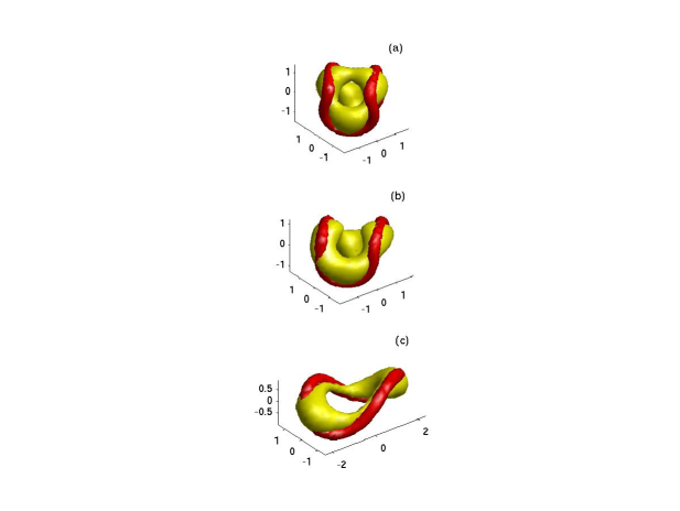
Figure 1: The charge density isosurface and position-curve $\psi_{3}=-0.8$ of the $N=3$ generalized Skyrmions: for (a) $\alpha=0$, (b) $\alpha=0.2$, and (c) $\alpha=0.4$.

For $N\geq 3$, the picture is less straightforward, with the Skyrmions having at most discrete symmetry. We look in detail at the cases $N=3$ and $N=4$. The 3-Skyrmion (for $\alpha=0$) has energy $E=3.4386$ and tetrahedral symmetry BTC90 ; BS02 ; in particular, a typical constant-${\cal B}$ surface resembles a tetrahedron. It is also useful to plot the curve in ${\bf R}^{3}$ where $\psi_{3}=-1$, or equivalently where $Z^{1}=0$ and $|Z^{2}|=1$; in the Faddeev-Skyrme system, this curve may be interpreted as the position of the string-like Hopf Skyrmion BS99 . Each plot in Figure 1 depicts the surface ${\cal B}({\bf x})=(\max{\cal B})/2$, with the ‘thickened’ curve $\psi_{3}=-0.8$ strung around it; subfigure (a) is for $\alpha=0$, (b) is for $\alpha=0.2$, and (c) is for $\alpha=0.4$. We see that as $\alpha$ increases from zero, the tetrahedral Skyrmion transforms into a twisted torus or loop (see also the pictures in BS99 for the $\alpha=1$ case). The tetrahedral symmetry is broken to the subgroup $D_{2}$. The normalized energy $E(\alpha)$ again has a quadratic dependence on $\alpha$: $E(\alpha)\approx 3.4386-0.60\,\alpha^{2}$.

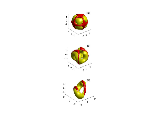
Figure 2: The charge density isosurface and position-curve $\psi_{3}=-0.8$ of the $N=4$ generalized Skyrmions: for (a) $\alpha=0$, (b) $\alpha=0.35$, and (c) $\alpha=0.4$.

Finally, let us look at the case $N=4$. The 4-Skyrmion (for $\alpha=0$) resembles a cube BTC90 ; BS02 : see Figure 2(a), where the same quantities are plotted as in Figure 1. As $\alpha$ increases, the minimum-energy configuration becomes a closed loop strung along eight edges of the cube (Figure 2(b), for $\alpha=0.35$), which then flattens as $\alpha$ increases further. When $\alpha=1$, one again gets a twisted circular loop, with the twisting being greater than in the $N=3$ case (see also the pictures in BS99 ).

We have seen that the Skyrme model and the Skyrme-Faddeev-Hopf system may be regarded as members of a one-parameter family of generalized Skyrme systems; and the topological-soliton solutions of all these systems, although rather different in appearance, are all closely-related to one another. A recent paper KS04 has pointed out a similarity between sphaleron solutions of the Skyrme system and axially-symmetric Hopf solitons, especially as the winding number $N$ increases. These solutions are unstable (saddle-points of their respective energy functionals); and this connection between Skyrmions and Hopf solitons is quite different from the one described above. It may be of interest, however, to investigate sphaleron-type solutions of the family of Skyrme systems, and see how they depend on the family parameter $\alpha$.

Note added in proof. A similar family arises from considering bundles of strings [S. Nasir and A. J. Niemi, Mod. Phys. Lett. A 17, 1445 (2002)]. The author is grateful to Prof. Niemi for correspondence regarding this.

- (1) N S Manton and P M Sutcliffe, Topological Solitons. (Cambridge University Press, Cambridge, 2004).
- (2) R A Battye and P M Sutcliffe, Skyrmions, Fullerines and Rational Maps. Rev Math Phys 14 (2002) 29–85.
- (3) E Braaten, S Townsend and L Carson, Novel structure of static multisoliton solutions in the Skyrme model. Phys Lett B 235 (1990) 147–152.
- (4) R A Battye and P M Sutcliffe, Solitons, Links and Knots. Proc Roy Soc Lond A 455 (1999) 4305–4331.
- (5) E Babaev, L Faddeev and A J Niemi, Hidden symmetry and duality in a charged two-condensate Bose system. Phys Rev B 65 (2002) 100512.
- (6) W J Zakrzewski, Classical solutions of some -like models. Lett Math Phys 12 (1986) 283.
- (7) N S Manton, Geometry of Skyrmions. Commun Math Phys 111 (1987) 469–478.
- (8) L Faddeev, Quantisation of Solitons [Preprint IAS Print-75-QS70, Princeton]; Lett Math Phys 1 (1976) 289.
- (9) L Faddeev and A J Niemi, Stable knot-like structures in classical field theory. Nature 387 (1997) 58–61.
- (10) J Gladikowski and M Hellmund, Static solitons with nonzero Hopf number. Phys Rev D 56 (1997) 5194–5199.
- (11) J Hietarinta and P Salo, Faddeev-Hopf knots: dynamics of linked un-knots. Phys Lett B 451 (1999) 60–67.
- (12) R S Ward, Hopf solitons on and . Nonlinearity 12 (1999) 241–246.
- (13) R S Ward, The interaction of two Hopf solitons. Phys Lett B 473 (2000) 291–296.
- (14) P van Baal and A Wipf, Classical gauge vacua as knots. Phys Lett B 515 (2001) 181–184.
- (15) S Krusch and P M Sutcliffe, Sphalerons in the Skyrme model. hep-th/0407002