SUSY-hierarchy of one-dimensional reflectionless potentials

Abstract

A class of one-dimensional reflectionless potentials is studied. It is found, that all possible types of the reflectionless potentials can be combined into one SUSY-hierarchy with a constant potential. An approach for determination of a general form of the reflectionless potential on the basis of construction of such a hierarchy by the recurrent method is proposed. A general integral form of interdependence between superpotentials with neighboring numbers of this hierarchy, opening a possibility to find new reflectionless potentials, is found and has a simple analytical view. It is supposed that any possible type of the reflectionless potential can be expressed through finite number of elementary functions (unlike some presentations of the reflectionless potentials, which are constructed on the basis of soliton solutions or are shape invariant in one or many steps with involving scaling of parameters, and are expressed through series). An analysis of absolute transparency existence for the potential which has the inverse power dependence on space coordinate (and here tunneling is possible), i. e. which has the form $V(x)=\pm\alpha/|x-x_{0}|^{n}$ (where $\alpha$ and $x_{0}$ are constants, $n$ is natural number), is fulfilled. It is shown that such a potential can be reflectionless at $n=2$ only. A SUSY-hierarchy of the inverse power reflectionless potentials is constructed. Isospectral expansions of this hierarchy is analyzed.

1 Introduction

The tunneling effect had considered else at the time of formulation of main principles of quantum mechanics and has been studied many years. Nevertheless, a lot of papers down to last days are directed to research of some its properties, which look rather unusual from the point of view of common sense (for example, resonant tunneling, reinforcement of penetrability of a barrier and violation of tunneling symmetry in opposite directions in the propagation of a system of several particles, absolute transparency for sub-barrier energies and reflection for above-barrier energies).

Original methods are developed with a purpose to understand such properties more deeply. Here, methods of supersymmetric quantum mechanics (SUSY QM) allow to find types of quantum systems (both in the region of continuous energy spectrum, and in discrete one), which potentials have penetrability coefficient equal to one for particle propagation through them both at separate levels, and in continuous range of the energy spectra. In the first case one can speak about resonant tunneling. In the second case the quantum systems and their potentials are named as reflectionless or absolutely transparent Zakhariev.1993.PHLTA .

A phenomenon of the resonant tunneling and, especially, papers directed to study of its demonstration in the concrete physical tasks, cause a significant interest Saito.1994.JCOME . But the reflectionless potentials having the penetrability coefficient, practically equal to one in a whole range of the continuous energy spectrum, are more unusual and, apparently, have other reasons of their existence. The reflectionless potentials can be investigated by methods of direct and inverse problems. Here, we should like to note both the monograph Chadan.1995 , and the excellent reviews Zakhariev.1994.PEPAN ; Zakhariev.1999.PEPAN , where both methods for detailed study of the properties of the reflectionless one- and multichannel quantum systems (mainly, in the region of the discrete energy spectrum), and approaches simple enough for their qualitative understanding are presented. All these methods have found their application in the scattering theory (both in the direct problem, and in the inverse one).

On the other side, the SUSY QM methods propose own approach for studying the properties of the reflectionless potentials. A considerable contribution is made by the papers, where the shape invariant potentials in one and many steps with involving scaling of parameters or their other transformations are studied (for example, see Khare.1993.JPAGB ; Balantekin.1997.PHRVA ). As a separate direction one can note the papers on study of self-similar potentials of Shabat and Spiridonov Shabat.1992.INPEE ; Spiridonov.1992.PRLTA ; Barclay.1993.PHRVA , concerned with $q$-supersymmetry Spiridonov.1992.MPLAE . The review Cooper.1995.PRPLC is the best (in my opinion).

Note, that the supersymmetric methods are less developed for study of the properties of the quantum systems in the region of the continuous energy spectrum (here, because of different boundary conditions, normalization conditions the interdependences between wave functions, energy spectra for the SUSY-partners systems can be qualitatively differed from similar interdependences of such spectral characteristics in the region of the discrete energy spectra). The different classes of the reflectionless potentials are opened by use of the different methods and a question about the account of all possible types of the reflectionless potentials (and, probably, about their classification) is appeared. A lot of known reflectionless potentials is concerned with soliton solutions in the inverse problem approach (for example, in the monography Zakhariev.1985 they are introduced as soliton solutions), and also with the soliton solutions in the SUSY QM approach (one- and many steps solutions, self-similar potentails of Shabat and Spiridonov, Rosen-Morse potentials with their $q$-deformation), where the absolute transparency is concerned with the above-barrier propagation, whereas considerably more rare is the reflectionless potential with a barrier above asymptotic tails, where the absolute transparency is observed in the sub-barrier tunneling. Many of known reflectionless potentials are expressed with use of series of a rather complicated form, and any found reflectionless potential in a simple analytical form can be useful by its clearness for the qualitative analysis of the properties of the reflectionless quantum systems.

In this paper we propose a way for determination of a general form of the one-dimensional reflectionless potential on the basis of construction of SUSY-hierarchy, which contains a constant potential. In obtaining of the hierarchy we try to take into account all possible types of the potentials, which belong to it. In the construction of the hierarchy we use a recurrent way, trying to not involve an analysis of an obvious form of wave functions (because of an influence of the boundary conditions, the normalization conditions on them can be essential). We suppose, that knowledge of such a hierarchy will allow to determine all possible types of the reflectionless potentials, and in such a case one can explain a nature of the absolute transparency of any reflectionless potential by its SUSY-connection with the constant potential through the considered SUSY-hierarchy. Such a definition of the reflectionless potentials looks more expanded, than the cases of the reflectionless soliton potentials (for example, see Zakhariev.1985 ) or the shape invariant reflectionless potentials.

In the construction of the considered SUSY-hierarchy all found by us reflectionless potentials have simple analytical forms and are expressed through elementary functions. According to the analysis, the complete SUSY-hierarchy includes both the reflectionless potentials constructed on a basis of the soliton solutions, and a set of the shape invariant reflectionless potentials, many from which are expressed with use of series. It results us to the idea that any reflectionless potential can be presented in a simple analytical form through finite number of elementary functions, that for any reflectionless potential with a known complicated representation in form of series there is another analytical representation in a simple form with use of elementary functions. However, one can make a final conclusion after a detailed analysis of all possible types of the reflectionless potentials (that we leave for future research). The simple evident representation of the reflectionless potentials is useful, because it, undoubtedly, will result to easier study of such potentials and, as result, to deeper understanding of the resonant tunneling, the absolute transparency and other unusual properties of tunneling.

We continue an analysis (started in Maydanyuk.2004.PAST.refl ) of the quantum systems with a completely continuous energy spectrum, which potentials have the inverse power dependence on space coordinate (here, the absolute transparency is possible during tunneling). We propose an approach for construction of the SUSY-hierarchy of the reflectionless inverse power potentials (obtained at the first time), and also we construct other special cases of SUSY-hierarchies of the reflectionless potentials.

For the first time we obtain some types of the reflectionless potentials, which have a simple analytical form, are expressed with use of the elementary functions and (at $x>0$) qualitatively remind a radial potential of interaction of particles with spherical nuclei in their elastic scattering (or in a decay of compound spherical systems).

We point out a possibility of construction of space asymmetric reflectionless potentials.

2 Interdependences between spectral characteristics of potentials-partners

Let’s consider an one-dimensional case of movement of a particle with mass $m$ in a potential field $V(x)$. We introduce the operators $A$ and $A^{+}$ of the following form:

$$\begin{array}[]{ll}A=\displaystyle\frac{\hbar}{\sqrt{2m}}\displaystyle\frac{d}{dx}+W(x),&A^{+}=-\displaystyle\frac{\hbar}{\sqrt{2m}}\displaystyle\frac{d}{dx}+W(x),\end{array}$$ (1)

where $W(x)$ is the function defined in the whole space region $x$. Let’s assume, that this function is continuous in the whole region of its definition except for several possible points of discontinuity. On the basis of the operators $A$ and $A^{+}$ one can construct two Hamiltonians for movement of this particle inside two different potentials $V_{1}(x)$ and $V_{2}(x)$:

$$\begin{array}[]{l}H_{1}=A^{+}A=-\displaystyle\frac{\hbar^{2}}{2m}\displaystyle\frac{d^{2}}{dx^{2}}+V_{1}(x),\\ H_{2}=AA^{+}=-\displaystyle\frac{\hbar^{2}}{2m}\displaystyle\frac{d^{2}}{dx^{2}}+V_{2}(x),\end{array}$$ (2)

where the potentials $V_{1}(x)$ and $V_{2}(x)$ are determined as follows:

$$\begin{array}[]{ll}V_{1}(x)=W^{2}(x)-\displaystyle\frac{\hbar}{\sqrt{2m}}\displaystyle\frac{dW(x)}{dx},&V_{2}(x)=W^{2}(x)+\displaystyle\frac{\hbar}{\sqrt{2m}}\displaystyle\frac{dW(x)}{dx}.\end{array}$$ (3)

In accordance with SUSY QM theory Cooper.1995.PRPLC , the function $W(x)$ is named as superpotential, whereas the potentials $V_{1}(x)$ and $V_{2}(x)$ are named as supersymmetric potentials - partners (or SUSY potentials - partners). A construction of the Hamiltonians of two quantum systems on the basis of the same operators $A$ and $A^{+}$ interrelates dependence between spectral characteristics (spectra of energy, wave functions) of these systems. One can see a reason of such interdependence in that two potentials $V_{1}(x)$ and $V_{2}(x)$ are connected through one function $W(x)$:

$$V_{2}(x)=V_{1}(x)+2\displaystyle\frac{\hbar}{\sqrt{2m}}\displaystyle\frac{dW(x)}{dx}.$$ (4)

2.1 Systems with discrete and continuous energy spectra

If the energy spectra of two considered systems are discrete, then one can write:

$$\begin{array}[]{l}H_{1}\varphi^{(1)}_{n}=A^{+}A\varphi^{(1)}_{n}=E^{(1)}_{n}\varphi^{(1)}_{n},\\ H_{2}\varphi^{(2)}_{n}=AA^{+}\varphi^{(2)}_{n}=E^{(2)}_{n}\varphi^{(2)}_{n},\end{array}$$ (5)

where $E^{(1)}_{n}$ and $E^{(2)}_{n}$ are the energy levels with number $n$ ($n$ is natural number) for two systems with potentials $V_{1}(x)$ and $V_{2}(x)$, $\varphi^{(1)}_{n}$ and $\varphi^{(2)}_{n}$ are the wave functions (eigen-functions), corresponding to this levels. From here we obtain:

$$\begin{array}[]{l}H_{2}(A\varphi^{(1)}_{n})=AA^{+}A\varphi^{(1)}_{n}=E^{(1)}_{n}(A\varphi^{(1)}_{n}),\\ H_{1}(A^{+}\varphi^{(2)}_{n})=A^{+}AA^{+}\varphi^{(2)}_{n}=E^{(2)}_{n}(A^{+}\varphi^{(2)}_{n}).\end{array}$$ (6)

Let’s displace the potential $V_{1}(x)$ by such a way that $E^{1}_{0}=0$ (it does not influence on a relative arrangement of the levels in the energy spectra and shapes of the wave functions). Analyzing (6), one can obtain the following interdependences between the energy spectra and the wave functions (see Cooper.1995.PRPLC , p. 275–276):

$$\begin{array}[]{ll}E^{(1)}_{0}=0,&\varphi^{(2)}_{n}=(E^{(1)}_{n+1})^{-1/2}A\varphi^{(1)}_{n+1},\\ E^{(2)}_{n}=E^{(1)}_{n+1},&\varphi^{(1)}_{n+1}=(E^{(2)}_{n})^{-1/2}A^{+}\varphi^{(2)}_{n}\end{array}$$ (7)

(though other variants of the interdependences are possible also). Here, a normalization condition for the wave functions is taken into account for the discrete spectrum:

$$\begin{array}[]{ll}\displaystyle\int\bigl{|}\varphi^{(1)}_{n}(x)\bigr{|}^{2}\,dx=1,&\displaystyle\int|\varphi^{(2)}_{n}(x)|^{2}\,dx=1.\end{array}$$ (8)

If the energy spectra of two systems are continuous, then one can find the interdependences between their wave functions also. In this case one can rewrite the system (5) by such a way:

$$\begin{array}[]{l}H_{1}\varphi^{(1)}_{k}=A^{+}A\varphi^{(1)}_{k}=E^{(1)}_{k}\varphi^{(1)}_{k},\\ H_{2}\varphi^{(2)}_{k^{\prime}}=AA^{+}\varphi^{(2)}_{k^{\prime}}=E^{(2)}_{k^{\prime}}\varphi^{(2)}_{k^{\prime}},\end{array}$$ (9)

where $E^{(1)}_{k}$ and $E^{(2)}_{k^{\prime}}$ are the energy levels for two systems with the potentials $V_{1}(x)$ and $V_{2}(x)$, having the continuous spectra of values, $\varphi^{(1)}_{k}(x)$ and $\varphi^{(2)}_{k^{\prime}}(x)$, $k=\displaystyle\frac{1}{\hbar}\sqrt{2mE^{(1)}_{k}}$ and $k^{\prime}=\displaystyle\frac{1}{\hbar}\sqrt{2mE^{(2)}_{k^{\prime}}}$ are the wave functions and the wave vectors, corresponding to the levels $E^{(1)}_{k}$ and $E^{(2)}_{k^{\prime}}$. From (9) we obtain:

$$H_{2}(A\varphi^{(1)}_{k})=AA^{+}(A\varphi^{(1)}_{k})=A(A^{+}A\varphi^{(1)}_{k})=A(E^{(1)}_{k}\varphi^{(1)}_{k})=E^{(1)}_{k}(A\varphi^{(1)}_{k}).$$ (10)

And one can write:

$$\begin{array}[]{lcr}A\varphi^{(1)}_{k}(x)=C_{2}\varphi^{(2)}_{k^{\prime}}(x),&E^{(1)}_{k}=\displaystyle\frac{E^{(2)}_{k^{\prime}}}{C_{2}},&C_{2}=const.\end{array}$$ (11)

Considering the second expression of this system and taking into account the definitions of the wave vectors $k$ and $k^{\prime}$, one can obtain the constant $C_{2}$. Taking into account (9), we write:

$$H_{1}(A^{+}\varphi^{(2)}_{k^{\prime}})=A^{+}AA^{+}\varphi^{(2)}_{k^{\prime}}=A^{+}(E^{(2)}_{k^{\prime}}\varphi^{(2)}_{k^{\prime}})=E^{(2)}_{k^{\prime}}(A^{+}\varphi^{(2)}_{k^{\prime}}),$$ (12)

and find:

$$\begin{array}[]{lcr}A^{+}\varphi^{(2)}_{k^{\prime}}(x)=C_{1}\varphi^{(1)}_{k}(x),&E^{(2)}_{k^{\prime}}=\displaystyle\frac{E^{(1)}_{k}}{C_{1}},&C_{1}=\displaystyle\frac{1}{C_{2}}=\displaystyle\frac{E^{(1)}_{k}}{E^{(2)}_{k^{\prime}}}=\displaystyle\frac{{k}^{2}}{{k^{\prime}}^{2}}.\end{array}$$ (13)

So, we have received the following interdependences between the wave functions and the energy levels for SUSY systems-partners in the continuous energy spectra:

$$\begin{array}[]{lcr}\varphi^{(1)}_{k}(x)=\displaystyle\frac{{k^{\prime}}^{2}}{{k}^{2}}A^{+}\varphi^{(2)}_{k^{\prime}}(x),&\varphi^{(2)}_{k^{\prime}}(x)=\displaystyle\frac{{k}^{2}}{{k^{\prime}}^{2}}A\varphi^{(1)}_{k}(x),&E^{(1)}_{k}=\displaystyle\frac{{k}^{2}}{{k^{\prime}}^{2}}E^{(2)}_{k^{\prime}}.\end{array}$$ (14)

One can see that lack of coincidence of the levels of the continuous energy spectra of SUSY systems-partners is possible (unlike the SUSY systems-partners with the discrete spectra). For determination of the exact interdependence between coefficients $k$ and $k^{\prime}$ it is necessary to use the normalization condition of the wave functions (for the continuous energy spectra) with taking into account of boundary conditions.

2.2 Interdependences between coefficients of penetrability and reflection

The SUSY QM methods allow to find the interdependences between coefficients of penetrability and reflection for two SUSY systems-partners in the regions of the continuous energy spectra (for example, see Cooper.1995.PRPLC , p. 278–279). Let the superpotential $W(x)$ and the potentials $V_{1}(x)$ and $V_{2}(x)$ converge at $x\to\pm\infty$ to finite limits:

$$\begin{array}[]{ll}W(x)\to W_{\pm},&V_{1}(x)=V_{2}(x)\to W^{2}_{\pm}.\end{array}$$ (15)

Let’s consider a propagation of a plane wave $e^{ik_{-}x}$ in the positive direction along the axis $x$ in the fields of the potentials $V_{1}(x)$ and $V_{2}(x)$ (we assume, that the propagation inside these two potentials occurs along identical levels $E^{(1)}$ and $E^{(2)}$). The incident wave from the left gives transmitted waves $T_{1}(k_{-},k_{+})e^{ik_{+}x}$ and $T_{2}(k_{-},k_{+})e^{ik_{+}x}$, and also reflected waves $R_{1}(k_{-})e^{-ik_{-}x}$ and $R_{2}(k_{-})e^{-ik_{-}x}$. We have:

$$\begin{array}[]{ll}\varphi^{(1)}(k,x\to-\infty)\to N_{1}(e^{ik_{-}x}+R_{1}e^{-ik_{-}x}),&\varphi^{(1)}(k,x\to+\infty)\to N_{1}T_{1}e^{ik_{+}x},\\ \varphi^{(2)}(k,x\to-\infty)\to N_{2}(e^{ik_{-}x}+R_{2}e^{-ik_{-}x}),&\varphi^{(2)}(k,x\to+\infty)\to N_{2}T_{2}e^{ik_{+}x},\end{array}$$ (16)

where $k$, $k_{-}$ and $k_{+}$ are determined by such a way:

$$\begin{array}[]{lcr}k=\displaystyle\frac{1}{\hbar}\sqrt{2mE},&k_{-}=\displaystyle\frac{1}{\hbar}\sqrt{2m(E-W^{2}_{-})},&k_{+}=\displaystyle\frac{1}{\hbar}\sqrt{2m(E-W^{2}_{+})},\end{array}$$ (17)

and the coefficients $N_{1}$ and $N_{2}$ can be found from the normalization conditions with taking into account of the potentials forms and the boundary conditions.

Using the interdependences (14) between the wave functions of two systems with the continuous spectra, we write:

$$\begin{array}[]{l}e^{ik_{-}x}+R_{1}e^{-ik_{-}x}=C_{2}N_{2}\biggl{[}\biggl{(}-\displaystyle\frac{ik_{-}\hbar}{\sqrt{2m}}+W_{-}\biggr{)}e^{ik_{-}x}+\biggl{(}\displaystyle\frac{ik_{-}\hbar}{\sqrt{2m}}+W_{-}\biggr{)}e^{-ik_{-}x}R_{2}\biggr{]},\\ T_{1}e^{ik_{+}x}=C_{2}N_{2}\biggl{(}-\displaystyle\frac{ik_{+}\hbar}{\sqrt{2m}}+W_{+}\biggr{)}e^{ik_{+}x}T_{2},\end{array}$$ (18)

where $C_{2}$ is a constant determined in (13). Equating items in (18) at the same exponents, one can find:

$$\begin{array}[]{ll}C_{2}N_{2}=\displaystyle\frac{1}{W_{-}-\displaystyle\frac{ik_{-}\hbar}{\sqrt{2m}}},&\\ R_{1}(k_{-})=R_{2}(k_{-})\displaystyle\frac{W_{-}+\displaystyle\frac{ik_{-}\hbar}{\sqrt{2m}}}{W_{-}-\displaystyle\frac{ik_{-}\hbar}{\sqrt{2m}}},&T_{1}(k_{-},k_{+})=T_{2}(k_{-},k_{+})\displaystyle\frac{W_{+}-\displaystyle\frac{ik_{+}\hbar}{\sqrt{2m}}}{W_{-}-\displaystyle\frac{ik_{-}\hbar}{\sqrt{2m}}}.\end{array}$$ (19)

The expressions (19) show the interdependences between amplitudes of the transmission and the reflection for SUSY systems-partners. Coefficients of the penetrability and the reflection for the potentials $V_{1}(x)$ and $V_{2}(x)$ can be calculated as squares of modules of the amplitudes of the transmission and the reflection.

2.3 Isospectral potentials

If we know the potential $V_{1}(x)$ only, then we can find the superpotential $W(x)$ by solving the first equation of the system (3). It is the differential equation of the first order. One can calculate the function $W(x)$ with an accuracy to one arbitrary constant of integration, which can be considered as a free parameter. Therefore, the function $W(x)$ is ambiguously determined. Generally, changing this free parameter, one can change a form of the function $W(x)$ without displacement of the levels in the energy spectrum and without change of a form of the potential $V_{1}(x)$.

According to (4), the potential $V_{2}(x)$ is expressed through $V_{1}(x)$ and derivative of $W(x)$ on coordinate. As the first equation of the system (3) is nonlinear, generally we can not speak that change of the considered above free parameter, resulting in the change of the superpotential $W(x)$, does not change the potential $V_{2}(x)$. On the other side, one can change the form of the potential - partner $V_{2}(x)$ by changing this parameter. Therefore, one can construct a set of potentials which have identical spectra of energy, different shapes and are named as isospectral potentials. As a confirmation of existence of the isospectral potentials, there is a beautiful example of one-parameter family of the one-dimensional isospectral potentials constructed on the basis of the oscillator potential and having identical equidistant spectrum of energy (see Cooper.1995.PRPLC , p. 326).

Let’s assume that the potential $V_{1}(x)$ is known and defined uniquely. Then we make the following conclusions:

• All possible types of the potentials $V_{2}(x)$, which are SUSY-partners to the potential $V_{1}(x)$, make one-parameter set $\mathcal{A}$ of the isospectral potentials (connected through one free parameter).

• Any potential $V_{2}(x)$, which is the SUSY-partner to the potential $V_{1}(x)$, belongs to this one-parameter set $\mathcal{A}$ of the isospectral potentials.

• One can suppose that any potential $V_{2}(x)$, which belongs to one-parameter set $\mathcal{A}$ of the isospectral potentials, is the SUSY-partner to the potential $V_{1}(x)$.

If the third item is carried out, then we come to analogy (one-to-one relationship) between one-parameter set of the isospectral potentials and the set of all possible types of the potentials, which are the SUSY-partners to one uniquely chosen potential. This analogy is obtained for the first time (though some dependences between these two sets were studied earlier). On its basis one can propose a choice of the parameter, concerning which the set of the one-parameter isospectral potentials is determined.

These reasoning are fulfilled both for systems with the discrete spectra of energy, and for systems with the continuous spectra of energy. They can be continued if to consider SUSY-hierarchy, to which the potentials $V_{1}(x)$ and $V_{2}(x)$ belong. So, finding possible types of the potentials - partners to the potential $V_{2}(x)$, we obtain a set new isospectral potentials $V_{3}(x)$, which are determined relatively the potential $V_{2}(x)$ and connected among themselves through one free parameter or determined relatively the initial potential $V_{1}(x)$ and connected among themselves through two independent free parameters.

Thus, we come to the conclusion about that some isospectral potentials are connected through only one independent free parameter, others isospectral potentials — through two independent free parameters, third — through three and so on (another approach to a construction of one- and many-parameter families of the isospectral potentials, where an analysis of an obvious form of wave functions is used, can be found in Cooper.1995.PRPLC , p. 323–329, with references to other papers).

3 Search of a general form of the reflectionless potential

According to (19), if we know a reflectionless potential (its reflection coefficient is equal to zero), than its SUSY potentials-partners can be also reflectionless.

Rule : two potentials $V_{1}(x)$ and $V_{2}(x)$ are reflectionless only when:

• these potentials are SUSY potentials-partners;

• asymptotic expressions of wave functions for both potentials have the form (16) (it is pointed out for the first time).

Using this natural rule and knowing a form of one reflectionless potential only, one can construct a set of new reflectionless potentials. Let’s apply such an approach to construction of the new reflectionless potentials, having taken as first the constant potential of the form:

$$V(x)=A^{2}=\mbox{const}$$ (20)

(we study the cases $A^{2}\leq 0$ and $A^{2}\geq 0$ at $A^{2}\in Re$). A plane wave $e^{ikx}$ (where $k$ is a wave vector determined at $E-V$) in the field of such potential does not meet an obstacle during its propagation. One can think that the potential (20) is reflectionless for the propagation of this wave (one can make sure in this by calculating the coefficients of the penetrability and the reflection).

If to construct SUSY-hierarchy, which has the potential (20), than only those potentials of such hierarchy are reflectionless, the asymptotic forms of the wave functions for which look like (16). All such potentials make one SUSY-hierarchy of the reflectionless potentials. Here, a reason of the absolute transparency of any such potential can be seen in its SUSY-interrelation with the constant potential.

4 Potentials-partners to the constant potential

Let’s assume, that the SUSY-hierarchy for the potential (20) is constructed. Let this potential be $V_{n}(x)$ with number $n$ in this hierarchy. We shall find the nearest potentials to it in this hierarchy, i. e. its potentials - partners.

4.1 The potentials-partners with a number “up”

At first we shall find the potential - partner $V_{n+1}(x)$ with the number “up”, i. e. when interdependence between these potentials has a form:

$$\begin{array}[]{ll}V_{n}(x)=W_{n}^{2}(x)-\displaystyle\frac{\hbar}{\sqrt{2m}}\displaystyle\frac{dW_{n}(x)}{dx},&V_{n+1}(x)=W_{n}^{2}(x)+\displaystyle\frac{\hbar}{\sqrt{2m}}\displaystyle\frac{dW_{n}(x)}{dx}.\end{array}$$ (21)

Taking into account (20), we write the differential equation for calculating superpotential $W_{n}(x)$:

$$W_{n}^{2}(x)-\displaystyle\frac{\hbar}{\sqrt{2m}}\displaystyle\frac{dW_{n}(x)}{dx}=A^{2}.$$ (22)

Introduce designation:

$$\alpha=\displaystyle\frac{\hbar}{\sqrt{2m}},$$ (23)

and solve the equation (22). At $W_{n}^{2}(x)=A^{2}$ we obtain:

$$V_{n+1}(x)=W_{n}^{2}(x)=V_{n}(x)=A^{2}.$$ (24)

We see that in this case the potential $V_{n}(x)$ is supersymmetric to itself.

At $W_{n}^{2}(x)\neq A^{2}$ we obtain:

$$\int dx=\alpha\displaystyle\int\displaystyle\frac{dW_{n}(x)}{W_{n}^{2}(x)-A^{2}}.$$ (25)

We find a dependence of the function $W_{n}$ on $x$. Therefore, we have the indefinite integral, with taking into account a constant of integration. At integration of this equation we obtain three different cases.

1) The case $A=0$. Then:

$$W_{n}(x)=-\displaystyle\frac{\alpha}{x+x_{0}},\mbox{ and }x+x_{0}\neq 0.$$ (26)

Here, the constant of integration $x_{0}$ is introduced.

2) The case $A\neq 0$ and $A^{2}>0$. Then:

$$A^{2}=(\rho e^{i\phi})^{2}=\rho^{2}e^{2i\phi}=+\rho^{2}=|A|^{2},$$ (27)

$$\left\{\begin{array}[]{ll}\displaystyle\frac{W_{n}-|A|}{W_{n}+|A|}=+e^{\displaystyle\frac{2|A|}{\alpha}(x+x_{0})},&\mbox{ at }|W_{n}|>|A|;\\ \displaystyle\frac{W_{n}-|A|}{W_{n}+|A|}=-e^{\displaystyle\frac{2|A|}{\alpha}(x+x_{0})},&\mbox{ at }|W_{n}|<|A|.\end{array}\right.$$ (28)

Let’s consider the first equation of this system. At $x+x_{0}\neq 0$ its solution has a form:

$$\begin{array}[]{l}W_{n}(x)=-|A|\coth\biggl{(}{\displaystyle\frac{|A|}{\alpha}(x+x_{0})}\biggr{)}.\end{array}$$ (29)

At $x+x_{0}=0$ two cases are possible:

$$\begin{array}[]{ccl}|A|=0&\Longrightarrow&\mbox{ false};\\ W_{n}(x\to-x_{0})\to\pm\infty&\Longrightarrow&\mbox{ true}.\end{array}$$

The first condition is not carried out, because of we study the case $A\neq 0$. The second condition is carried out automatically as a limit of the expression (29) and satisfies to the condition: $|W_{n}(x)|>|A|$. Therefore, one can remove the restriction $x+x_{0}\neq 0$ on the solution (29).

The second equation of the system (28) gives such result:

$$W_{n}(x)=-|A|\tanh\biggl{(}\displaystyle\frac{|A|}{\alpha}(x+x_{0})\biggr{)}$$ (30)

and does not use the restriction $x\neq-x_{0}$ also (here, $W_{n}(x)\to 0$ at $x+x_{0}\to 0$).

3) The case $A\neq 0$ and $A^{2}<0$. Then:

$$A^{2}=(\rho e^{i\phi})^{2}=\rho^{2}e^{2i\phi}=-\rho^{2}=-|A|^{2},$$ (31)

$$W_{n}(x)=|A|\tan\biggl{(}\displaystyle\frac{|A|}{\alpha}(x+x_{0})\biggr{)}.$$ (32)

So, we have obtained five solutions of the function $W_{n}(x)$:

$$W_{n}(x)=\left\{\begin{array}[]{cl}\pm|A|=const;&\\ -\displaystyle\frac{\alpha}{x+x_{0}},&\mbox{for }A=0,W_{n}^{2}(x)\neq 0\mbox{ and }\\ &x+x_{0}\neq 0;\\ -|A|\coth\biggl{(}\displaystyle\frac{|A|}{\alpha}(x+x_{0})\biggr{)},&\mbox{for }A^{2}>0\mbox{ and }|W_{n}(x)|>|A|;\\ -|A|\tanh\biggl{(}\displaystyle\frac{|A|}{\alpha}(x+x_{0})\biggr{)},&\mbox{for }A^{2}>0\mbox{ and }|W_{n}(x)|<|A|;\\ |A|\tan\biggl{(}\displaystyle\frac{|A|}{\alpha}(x+x_{0})\biggl{)},&\mbox{for }A^{2}<0\mbox{ and }W_{n}^{2}(x)\neq A^{2},\end{array}\right.$$ (33)

where $x_{0}$ is the constant of integration (unique free parameter).

According to (21), the superpotential $W(x)$ uniquely defines the potential $V_{n+1}(x)$, which has five solutions:

$$\begin{array}[]{l}V_{n+1}(x)=\left\{\begin{array}[]{cl}A^{2},&\mbox{for }W^{2}_{n}(x)=A^{2};\\ \displaystyle\frac{2\alpha^{2}}{(x+x_{0})^{2}},&\mbox{for }A=0,W_{n}^{2}(x)\neq 0\mbox{ and }\\ &x+x_{0}\neq 0;\\ |A|^{2}\left(1+\displaystyle\frac{2}{\sinh^{2}\bigl{(}|A|(x+x_{0})/\alpha\bigr{)}}\right),&\mbox{for }A^{2}>0\mbox{ and }|W_{n}(x)|>|A|;\\ |A|^{2}\left(1-\displaystyle\frac{2}{\cosh^{2}\bigl{(}|A|(x+x_{0})/\alpha\bigr{)}}\right),&\mbox{for }A^{2}>0\mbox{ and }|W_{n}(x)|<|A|;\\ |A|^{2}\left(\displaystyle\frac{2}{\cos^{2}\bigl{(}|A|(x+x_{0})/\alpha\bigr{)}}-1\right),&\mbox{for }A^{2}<0\mbox{ and }W_{n}^{2}(x)\neq A^{2}.\end{array}\right.\end{array}$$ (34)

4.2 The potentials-partners with a number “down”

Now we find a potential $V_{n-1}(x)$ with the number “down”, which is the SUSY-partner to the constant potential $V_{n}(x)$ of the form (20). An equation for determination of a superpotential $W_{n-1}(x)$, connecting $V_{n-1}(x)$ and $V_{n}(x)$, has a form:

$$W^{2}_{n-1}(x)+\alpha\displaystyle\frac{dW_{n-1}(x)}{dx}=A^{2}.$$ (35)

At replacement

$$\bar{\alpha}\to-\alpha.$$ (36)

this equation transforms into the equation (22). Then the solutions of the equation (33) become the solutions of the equation (35):

$$W_{n-1}(x)=\left\{\begin{array}[]{cl}\pm|A|=const;&\\ \displaystyle\frac{\alpha}{x+x_{0}},&\mbox{at }A=0,W_{n-1}^{2}(x)\neq 0\mbox{ and }\\ &x+x_{0}\neq 0;\\ |A|\coth\biggl{(}\displaystyle\frac{|A|}{\alpha}(x+x_{0})\biggr{)},&\mbox{at }A^{2}>0\mbox{ and }|W_{n-1}(x)|>|A|;\\ |A|\tanh\biggl{(}\displaystyle\frac{|A|}{\alpha}(x+x_{0})\biggr{)},&\mbox{at }A^{2}>0\mbox{ and }|W_{n-1}(x)|<|A|;\\ -|A|\tan\biggl{(}\displaystyle\frac{|A|}{\alpha}(x+x_{0})\biggl{)},&\mbox{at }A^{2}<0\mbox{ and }W_{n-1}^{2}(x)\neq A^{2},\end{array}\right.$$ (37)

where $x_{0}$ is the constant of integration (unique free parameter), and the solutions for $V_{n-1}(x)$ coincide with the solutions for $V_{n+1}(x)$:

$$V_{n-1}(x)=V_{n+1}(x).$$ (38)

So, we have obtained the SUSY potentials-partners to the constant potential (20). Note the following:

• All possible types of the SUSY potentials-partners with the numbers “up” and “down” to the constant potential are defined by the expressions (34) and (38). There are no any other type (with the exception of these five solutions) of the potential-partner to the constant potential (it is obtained for the first time).

• In order to find out, which potentials from the obtained above solutions are reflectionless, it is need to analyze an asymptotic form of wave functions of these potentials.

  • The first potential is constant. It is supersymmetric to itself, keeps a property of absolute transparency and does not give anything new.

  • The second potential has the inverse power dependence on coordinate. One can construct new reflectionless potentials on the basis of it (where there is a tunneling) and it will be studied in subsection 5.1.

  • The fourth potential is known in the literature as reflectionless potential (see p. 280 in Cooper.1995.PRPLC ). It is used often also in construction and analysis of one- and many-soliton reflectionless potentials (see p. 328 in Cooper.1995.PRPLC ).

  • If the fifth potential is determined on the whole axis $x$, then in a general case it has an infinite set of barriers (like $\delta$-barriers), and it is not clear, how to consider a directed motion of a particle (with tunneling) in the field of such potential. At limits $x\to\pm\infty$ this potential does not converges to unambiguous values. Therefore, its wave function does not have the unambiguous form in the asymptotic areas and is not reduced to the form (16) in a general case. Examples of this potential as potential-partner to the constant potential defined on the given finite region on $x$ is studied in literature (see p. 278–279 in Cooper.1995.PRPLC ).

  The second and third potentials as reflectionless are not found by us in other papers.

• At $x\to\pm\infty$ the wave functions tend to the form (16) only for those potentials, which have finite values in a whole region of their definition and converge to unique finite values at $x\to\pm\infty$. Therefore, for extraction of the reflectionless potentials from the considered above SUSY-hierarchy the analysis of the form of the wave function in the asymptotic areas can be replaced by the analysis of existence of the potential finiteness in the whole region of its definition and existence of its unique finite limits at $x\to\pm\infty$.

• One can see $x_{0}$ as a free parameter, changing which one can change the forms of the potentials (with displacement along the $x$ axis) without displacement of the levels in the energy spectra (such potentials make one-parameter set of isospectral potentials). Here, if the absolute transparency exists, then it is kept (in the regions of application of these potentials). The same situation exists in the one-parameter family of the isospectral potentials constructed on the basis of the analysis of wave functions (for example, see p. 326 and Fig. 7.1 in Cooper.1995.PRPLC ).

• All found reflectionless potentials have a simple analytical form and are expressed through elementary functions.

5 Construction of the SUSY-hierarchy of the reflectionless potentials

Consistently determining by a recurrent way the potentials belonging to one SUSY-hierarchy, which contains constant potential, and selecting the potentials of finite height with unique finite asymptotic limits from this hierarchy, one can find new types of the reflectionless potentials. Let’s consider some cases of the reflectionless SUSY-hierarchies.

5.1 Inverse power reflectionless potentials

Let’s analyze a case, when a potential having the inverse power dependence on spatial coordinate, can be reflectionless.

5.1.1 Potentials-partners to the constant potential

Let’s consider a superpotential of the form:

$$W(x)=\left\{\begin{array}[]{ll}\displaystyle\frac{-\alpha}{x-x_{0}},&\mbox{at }x<0;\\ \displaystyle\frac{-\alpha}{x+x_{0}},&\mbox{at }x>0;\end{array}\right.$$ (39)

where $\alpha>0$, $x_{0}>0$. According to (3), the function $W(x)$ uniquely defines the potentials-partners $V_{1}(x)$ and $V_{2}(x)$:

$$\mbox{for }x<0\left\{\begin{array}[]{l}V_{1}(x)=W^{2}(x)-\displaystyle\frac{\hbar}{\sqrt{2m}}\displaystyle\frac{dW(x)}{dx}=\displaystyle\frac{\alpha}{(x-x_{0})^{2}}\biggl{(}\alpha-\displaystyle\frac{\hbar}{\sqrt{2m}}\biggl{)},\\ V_{2}(x)=W^{2}(x)+\displaystyle\frac{\hbar}{\sqrt{2m}}\displaystyle\frac{dW(x)}{dx}=\displaystyle\frac{\alpha}{(x-x_{0})^{2}}\biggl{(}\alpha+\displaystyle\frac{\hbar}{\sqrt{2m}}\biggl{)};\end{array}\right.$$ (40)

$$\mbox{for }x>0\left\{\begin{array}[]{l}V_{1}(x)=W^{2}(x)-\displaystyle\frac{\hbar}{\sqrt{2m}}\displaystyle\frac{dW(x)}{dx}=\displaystyle\frac{\alpha}{(x+x_{0})^{2}}\biggl{(}\alpha-\displaystyle\frac{\hbar}{\sqrt{2m}}\biggl{)},\\ V_{2}(x)=W^{2}(x)+\displaystyle\frac{\hbar}{\sqrt{2m}}\displaystyle\frac{dW(x)}{dx}=\displaystyle\frac{\alpha}{(x+x_{0})^{2}}\biggl{(}\alpha+\displaystyle\frac{\hbar}{\sqrt{2m}}\biggl{)}.\end{array}\right.$$ (41)

From (40) and (41) one can see, that when the following condition

$$\alpha=\displaystyle\frac{\hbar}{\sqrt{2m}}$$ (42)

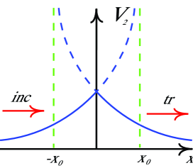
Figure 1: The barrier becomes reflectionless at $\alpha=\displaystyle\frac{\hbar}{\sqrt{2m}}$

is fulfilled, then the potential $V_{1}$ becomes zero. The coefficient of penetrability of this potential for a propagation of a plane wave is equal to one and, this sense, the potential $V_{1}(x)$ is reflectionless. The potential $V_{2}(x)$ is defined and is finited on the whole axis $x$, has a barrier with a finite top at $x=x_{0}$ and tends to zero in the asymptotic areas (see Fig. 1). Therefore, an unidirectional movement of the plane wave with tunneling in this potential is possible. According to (19), the coefficient of penetrability of this potential also is equal to one:

$$|T_{1}|^{2}=|T_{2}|^{2}=1.$$ (43)

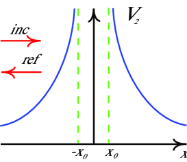
Figure 2: Absolute reflection at $x_{0}<0$

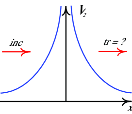
Figure 3: Boundary case at $x_{0}=0$

Note a property: the coefficient of penetrability for the reflectionless potential $V_{2}(x)$ does not changed with displacement of $x_{0}$ (at $x_{0}>0$). At $x_{0}<0$ there is a region $x\in]-|x_{0}|,+|x_{0}|[$, where this potential becomes indefinitely large and absolutely opaque (see Fig. 2). A case $x_{0}=0$ is boundary (see Fig. 3).

In more general case for the superpotential of such a form (where $\alpha>0$, $x_{0}>0$, $n$ is natural number):

$$W(x)=\left\{\begin{array}[]{ll}-\displaystyle\frac{\alpha}{|x-x_{0}|^{n}},&\mbox{at }x<0;\\ -\displaystyle\frac{\alpha}{|x+x_{0}|^{n}},&\mbox{at }x>0;\end{array}\right.$$ (44)

the potentials-partners $V_{1}(x)$ and $V_{2}(x)$ have the following form:

$$V_{1}(x)=\left\{\begin{array}[]{ll}\displaystyle\frac{\alpha}{(x-x_{0})^{2n}}\biggl{(}\alpha-\displaystyle\frac{\hbar n|x-x_{0}|^{n-1}}{\sqrt{2m}}\biggl{)},&\mbox{at }x<0;\\ \displaystyle\frac{\alpha}{(x+x_{0})^{2n}}\biggl{(}\alpha-\displaystyle\frac{\hbar n|x+x_{0}|^{n-1}}{\sqrt{2m}}\biggl{)},&\mbox{at }x>0;\\ \end{array}\right.$$ (45)

$$V_{2}(x)=\left\{\begin{array}[]{ll}\displaystyle\frac{\alpha}{(x-x_{0})^{2n}}\biggl{(}\alpha+\displaystyle\frac{\hbar n}{\sqrt{2m}}|x-x_{0}|^{n-1}\biggl{)},&\mbox{at }x<0;\\ \displaystyle\frac{\alpha}{(x+x_{0})^{2n}}\biggl{(}\alpha+\displaystyle\frac{\hbar n}{\sqrt{2m}}|x+x_{0}|^{n-1}\biggl{)},&\mbox{at }x>0.\end{array}\right.$$ (46)

The potential $V_{1}(x)$ is constant only at fulfillment of one condition: $n=0$ or $n=1$. The condition $n=0$ gives the trivial solution. At $n=1$ the potential $V_{2}(x)$ becomes reflectionless, if the condition (42) is fulfilled. If $n\neq 1$, then it is impossible to achieve a constancy of the potentials $V_{1}(x)$ or $V_{2}(x)$ by variation of the parameters $\alpha$ and $m$. At replacement of the sign for $W(x)$ the sign before the potentials $V_{1}(x)$ and $V_{2}(x)$ does not changed.

5.1.2 Construction of the hierarchy of the reflectionless inverse power potentials

One can construct hierarchy of the reflectionless potentials (where there is tunneling), which have the inverse power dependence on spatial coordinate. Let’s consider a potential of such form:

$$V_{n}(x)=\left\{\begin{array}[]{ll}\gamma\displaystyle\frac{\alpha^{2}}{(x-x_{0})^{2}},&\mbox{at }x<0;\\ \gamma\displaystyle\frac{\alpha^{2}}{(x+x_{0})^{2}},&\mbox{at }x>0.\end{array}\right.$$ (47)

We shall find for it a potential-partner $V_{n+1}(x)$ with a number “up”, which has the inverse power dependence also. For simplicity, we shall consider the potentials in the region $x>0$ only (solutions for the potentials in the region $x<0$ can be obtained by using of the replacement $x_{0}\to-x_{0}$). Write:

$$\begin{array}[]{l}V_{n}(x)=W_{n}^{2}(x)-\alpha\displaystyle\frac{dW_{n}(x)}{dx}=\displaystyle\frac{\gamma\alpha^{2}}{(x+x_{0})^{2}};\\ V_{n+1}(x)=W_{n}^{2}(x)+\alpha\displaystyle\frac{dW_{n}(x)}{dx}.\end{array}$$ (48)

From here we obtain the equation for calculation the $W_{n}(x)$:

$$\alpha\displaystyle\frac{dW_{n}(x)}{dx}=W_{n}^{2}(x)-\displaystyle\frac{\gamma\alpha^{2}}{(x+x_{0})^{2}}.$$ (49)

If to find the solution in the form:

$$W_{n}(x)=-\displaystyle\frac{\beta}{x+x_{0}},$$ (50)

then we obtain the following result:

$$\beta=\displaystyle\frac{\alpha}{2}\biggl{(}1\pm\sqrt{4\gamma+1}\biggr{)}.$$ (51)

Now we shall find the potential-partner $V_{n+1}(x)$. According to (48) and (50), we obtain:

$$V_{n+1}(x)=\biggl{(}1+\gamma\pm\sqrt{4\gamma+1}\biggr{)}\displaystyle\frac{\alpha^{2}}{(x+x_{0})^{2}}.$$ (52)

On the basis of this expression and (47) one can construct the recurrent formula for calculation of new inverse power potential with the numbers “up” and “down” in the SUSY-hierarchy on the basis of the known old potential (we write the potential on the whole axis $x$):

$$\begin{array}[]{ll}\gamma_{n\pm 1}=1+\gamma_{n}\pm\sqrt{4\gamma_{n}+1};&V_{n}(x)=\left\{\begin{array}[]{ll}\gamma_{n}\displaystyle\frac{\alpha^{2}}{(x-x_{0})^{2}},&\mbox{for }x<0;\\ \gamma_{n}\displaystyle\frac{\alpha^{2}}{(x+x_{0})^{2}},&\mbox{for }x>0.\end{array}\right.\end{array}$$ (53)

If to choose

$$\gamma_{n}=2,$$ (54)

than the potential (47) becomes reflectionless of the form (40) and (41). In such a case the expression (53) describes by the recurrent way the sequence of the reflectionless inverse power potentials with the following coefficients $\gamma$ (we write only first values):

$$\gamma=0,2,6,12,20,30,42...$$ (55)

and makes the SUSY-hierarchy (it is obtained for the first time).

Note, that this sequence contains natural numbers only!

5.1.3 A generalization on a spherically-symmetric case

The analysis, fulfilled above, of existence of the one-dimensional reflectionless potentials can be generalized on the spherically symmetric case (at $l=0$). Here, we consider the functions $W(r)$ and $V_{1,2}(r)$ for positive $r>0$ only. For $n=1$ we obtain:

$$\biggl{(}W(r)=\displaystyle\frac{-\alpha}{r+r_{0}}\biggr{)}\Longrightarrow\left\{\begin{array}[]{l}V_{1}(r)=\displaystyle\frac{\alpha}{(r+r_{0})^{2}}\biggl{(}\alpha-\displaystyle\frac{\hbar}{\sqrt{2m}}\biggl{)},\\ V_{2}(r)=\displaystyle\frac{\alpha}{(r+r_{0})^{2}}\biggl{(}\alpha+\displaystyle\frac{\hbar}{\sqrt{2m}}\biggl{)}.\end{array}\right.$$ (56)

At fulfillment (42) the potential $V_{1}(r)$ becomes zero, the potentials $V_{1}(r)$ and $V_{2}(r)$ — reflectionless, and a scattering of a particle on them — resonant.

5.2 A variety of SUSY-hierarchies

5.2.1 A hierarchy generated by the hyperbolic superpotential $W(x)\sim\coth{(x)}$

Let’s consider a superpotential of a form:

$$W_{n}(x)=|A|B\coth{\biggl{(}C\displaystyle\frac{|A|}{\alpha}(x+x_{0})\biggr{)}}.$$ (57)

We find potentials-partners connected by this superpotential:

$$\begin{array}[]{lcl}V_{n}(x)&=&|A|^{2}\left(B^{2}+\displaystyle\frac{B^{2}+BC}{\sinh^{2}\biggl{(}C\displaystyle\frac{|A|}{\alpha}(x+x_{0})\biggr{)}}\right),\\ V_{n+1}(x)&=&|A|^{2}\left(B^{2}+\displaystyle\frac{B^{2}-BC}{\sinh^{2}\biggl{(}C\displaystyle\frac{|A|}{\alpha}(x+x_{0})\biggr{)}}\right).\end{array}$$ (58)

We see, that the first item in the potentials-partners $V_{n}(x)$ and $V_{n+1}(x)$, connected through the superpotential of the form (57), does not changed. Then the following potentials in this hierarchy have the same first item. The constant potential can belong to such hierarchy only, when:

$$B^{2}=1.$$ (59)

One can use:

$$\begin{array}[]{ll}B=-1;&C>0.\end{array}$$ (60)

If to enter designations:

$$\begin{array}[]{ll}\beta_{n}=1-C,&\beta_{n+1}=1+C,\end{array}$$ (61)

then we obtain a general form of the potential belonging to the SUSY-hierarchy of potentials, connected through the superpotential (57):

$$\begin{array}[]{ll}V_{n}(x)=|A|^{2}\left(1+\displaystyle\frac{\beta_{n}}{\sinh^{2}\biggl{(}C\displaystyle\frac{|A|}{\alpha}(x+x_{0})\biggr{)}}\right);&\beta_{n+1}=2-\beta_{n}.\end{array}$$ (62)

One can find an useful interdependence between the potentials-partners:

$$V_{n+1}(x)=-V_{n}(x)+|A|^{2}\left(2+\displaystyle\frac{2}{\sinh^{2}\biggl{(}C\displaystyle\frac{|A|}{\alpha}(x+x_{0})\biggr{)}}\right).$$ (63)

If to take into account, that the constant potential (20) belongs to such hierarchy, than from (63) one can obtain its SUSY-partner coincided with the third solution of the system (34) at $C=1$. Thus, the SUSY-hierarchy, obtained by such a way, contains only two potentials, which are reflectionless:

$$\begin{array}[]{lcl}V_{n}(x)&=&|A|^{2};\\ V_{n\pm 1}(x)&=&|A|^{2}\left(1+\displaystyle\frac{2}{\sinh^{2}\biggl{(}C\displaystyle\frac{|A|}{\alpha}(x+x_{0})\biggr{)}}\right).\end{array}$$ (64)

One can see that there are no other potentials in this SUSY-hierarchy, with the exception of these two. The expression (63) corresponds to the definition of the shape invariant potentials (see Cooper.1995.PRPLC , p. 290, (96)).

On the other side, from (62), (60) and (61)) one can find a sequence of values of $\beta_{n}$ and $C$:

$$\begin{array}[]{lcl}\biggl{(}(\beta_{n}=0)\to(\beta_{n+1}=2)\to(\beta_{n+2}=0)\biggr{)}&\Longrightarrow&(\beta_{i}=0,2;\,C=1).\end{array}$$ (65)

We again come to the conclusion about the existence of only two reflectionless potentials in the considered hierarchy.

Property: if we add the following potential

$$V(x)=\displaystyle\frac{2|A|^{2}}{\sinh^{2}\biggl{(}\displaystyle\frac{|A|}{\alpha}(x+x_{0})\biggr{)}},$$

to the constant potential $V(x)=|A|^{2}$, then new potential remains reflectionless.

5.2.2 A hierarchy generated by the hyperbolic superpotential $W(x)\sim\tanh{(x)}$

Let’s find the potentials-partners connected by a superpotential of such a form:

$$W_{n}(x)=|A|B\tanh\biggl{(}C\displaystyle\frac{|A|}{\alpha}(x+x_{0})\biggr{)}.$$ (66)

We obtain:

$$\begin{array}[]{lcl}V_{n}(x)&=&|A|^{2}\left(B^{2}-\displaystyle\frac{B^{2}+BC}{\cosh^{2}\biggl{(}C\displaystyle\frac{|A|}{\alpha}(x+x_{0})\biggr{)}}\right),\\ V_{n+1}(x)&=&|A|^{2}\left(B^{2}-\displaystyle\frac{B^{2}-BC}{\cosh^{2}\biggl{(}C\displaystyle\frac{|A|}{\alpha}(x+x_{0})\biggr{)}}\right).\end{array}$$ (67)

Similarly the reasoning of the previous paragraph, we obtain:

$$\begin{array}[]{ll}B=-1;&C>0.\end{array}$$ (68)

If to enter the following designations:

$$\begin{array}[]{ll}\beta_{n}=1-C,&\beta_{n+1}=1+C,\end{array}$$ (69)

then we obtain recurrent dependences for description of a general form of the potential belonging to the SUSY-hierarchy with the superpotential (66):

$$\begin{array}[]{lcl}V_{n}(x)&=&|A|^{2}\left(1-\displaystyle\frac{\beta_{n}}{\cosh^{2}\biggl{(}C\displaystyle\frac{|A|}{\alpha}(x+x_{0})\biggr{)}}\right),\\ \beta_{n+1}&=&2-\beta_{n},\end{array}$$ (70)

and interdependence between the potentials-partners in this hierarchy:

$$V_{n+1}(x)=-V_{n}(x)+|A|^{2}\left(2-\displaystyle\frac{2}{\cosh^{2}\biggl{(}C\displaystyle\frac{|A|}{\alpha}(x+x_{0})\biggr{)}}\right).$$ (71)

If as one of such potentials to use the constant potential (20), then one can conclude that the SUSY-hierarchy, defined by such a way, contains only two reflectionless potentials of the form:

$$\begin{array}[]{lcl}V_{n}(x)&=&|A|^{2};\\ V_{n\pm 1}(x)&=&|A|^{2}\left(1-\displaystyle\frac{2}{\cosh^{2}\biggl{(}\displaystyle\frac{|A|}{\alpha}(x+x_{0})\biggr{)}}\right).\end{array}$$ (72)

One can find all possible values of the coefficient $\beta_{n}$:

$$\begin{array}[]{ll}\beta_{i}=0,2;&C=1.\end{array}$$ (73)

Property: if to subtract the potential of the form

$$V(x)=\displaystyle\frac{2|A|^{2}}{\cosh^{2}\biggl{(}\displaystyle\frac{|A|}{\alpha}(x+x_{0})\biggr{)}},$$

from the constant potential $V(x)=|A|^{2}$, then new potential remains reflectionless.

5.3 Methods

Now we shall be looking for an approach for calculation of all possible forms of potentials belonging to one SUSY-hierarchy, which contains a reflectionless potential $V_{n}(x)$. Let’s consider a sequence of the potentials of such hierarchy in a direction of numbers “up”. According to (3), we write:

$$V_{n+1}(x)=W_{n}^{2}(x)+\alpha\displaystyle\frac{dW_{n}(x)}{dx}=V_{n}(x)+2\alpha\displaystyle\frac{dW_{n}(x)}{dx}.$$ (74)

For the following numbers $n+1$… $n+m$ we obtain:

$$V_{n+m}(x)=V_{n}(x)+2\alpha\biggl{(}\displaystyle\frac{dW_{n}(x)}{dx}+\displaystyle\frac{dW_{n+1}(x)}{dx}+...+\displaystyle\frac{dW_{n+m-1}(x)}{dx}\biggr{)}.$$ (75)

5.3.1 A recurrent method of construction of the SUSY-hierarchy of the reflectionless potentials

The superpotential $W_{n+1}(x)$ can be expressed through $W_{n}(x)$:

$$W_{n+1}^{2}(x)-\alpha\displaystyle\frac{dW_{n+1}(x)}{dx}=W_{n}^{2}(x)+\alpha\displaystyle\frac{dW_{n}(x)}{dx}.$$ (76)

Using the function $W_{n}(x)$ with the number $n$ and solving the differential equation (76), one can find the function $W_{n+1}(x)$ with the number $n+1$. From the equation (76) one can see, that the function $W_{n+1}(x)$ of the form

$$W_{n+1}(x)=-W_{n}(x)$$ (77)

is a partial solution of this equation (in particular, this expression is carried out for the superpotentials (33) and (37) with numbers “up” and “down” concerning the constant potential). Knowing the partial solution decision for the function $W_{n+1}(x)$, one can find its general solution by a method described in the following subsection. Further, knowing the general form of the function $W_{n+1}(x)$, one can construct a new equation for determination of an unknown function $W_{n+2}(x)$. So, we obtain the recurrent approach for calculation of the general form of the function $W_{i}(x)$ with numbers from $n$ up to $n+m$ (i. e. we take into account all possible solutions). The determined superpotentials $W_{i}(x)$ allow to find potentials $V_{i}(x)$ with numbers from $n$ up to $n+m$:

$$V_{i}(x)=W_{i}^{2}(x)-\alpha\displaystyle\frac{dW_{i}(x)}{dx}$$ (78)

By such a way, one can construct a general form of the SUSY-hierarchy (it is necessary to take into account potentials with numbers “down”), if we know its one potential $V_{n}(x)$.

In order to construct the SUSY-hierarchy of the reflectionless potentials, it is need to use the constant potential (20) as the potential $V_{n}(x)$ and on the basis of the described above approach consistently to determine possible types of the potentials. Here, knowledge of wave functions of these potentials is not required. Further, from this set of the potentials it is need to select the reflectionless potentials, which are finite in whole axis $x$ and converge to uniquely finite limits in the asymptotic areas.

5.3.2 Search of a general form of the superpotential

We shall find a general solution of the equation (76). Let’s rewrite this equation by such a way:

$$\frac{dW(x)}{dx}-\displaystyle\frac{1}{\alpha}W^{2}(x)=-\displaystyle\frac{F(x)}{\alpha}.$$ (79)

This is the Ricatti equation. According to Tihonov.1998 (see p. 29), it is not integrated exactly. However, it has one property: if we know its one partial solution, then this equation can be reduced to the Bernoulli equation and one can find its general solution. Let we know its partial solution $\tilde{W}(x)$ (for example, see (77)). We change variable:

$$z(x)=W(x)-\tilde{W}(x).$$ (80)

Then one can transform the equation (79) into the following equation with new variables:

$$\frac{dz(x)}{dx}-\displaystyle\frac{2\tilde{W}(x)}{\alpha}z(x)-\displaystyle\frac{1}{\alpha}z^{2}(x)=0.$$ (81)

This is the Bernoulli equation. We change variable:

$$y(x)=z^{-1}=\displaystyle\frac{1}{z(x)}$$ (82)

and reduce this equation to such a form:

$$\frac{dy(x)}{dx}+\displaystyle\frac{2\tilde{W}(x)}{\alpha}y(x)=-\displaystyle\frac{1}{\alpha}.$$ (83)

In result, we obtain the general solution:

$$y(x)=e^{-\displaystyle\int\displaystyle\frac{2\tilde{W}(x)}{\alpha}dx}\biggl{(}C_{1}-\displaystyle\frac{1}{\alpha}\displaystyle\int e^{\displaystyle\int\displaystyle\frac{2\tilde{W}(x)}{\alpha}dx}dx\biggl{)},$$ (84)

where $C_{1}$ is a constant of integration (the indefinite integral is used). In the old variables the solution has the following form:

$$\begin{array}[]{lcl}W(x)&=&z(x)+\tilde{W}(x)=\displaystyle\frac{1}{y(x)}+\tilde{W}(x)=\displaystyle\frac{e^{\displaystyle\int\displaystyle\frac{2\tilde{W}(x)}{\alpha}dx}}{C_{1}-\displaystyle\frac{1}{\alpha}\displaystyle\int e^{\displaystyle\int\displaystyle\frac{2\tilde{W}(x)}{\alpha}dx}dx}+\\ &+&\tilde{W}(x).\end{array}$$ (85)

Using the different partial solutions $\tilde{W}(x)$, one can find new types of the reflectionless potentials, which have a simple analytical form. For the selected function $\tilde{W}(x)$ one can obtain the general form of the superpotential $W(x)$ and the potential-partner, which depend on the constant $C_{1}$. The constant $C_{1}$ plays a role of a free parameter, changing which, one can change the form of the superpotential and the potential-partner (such potentials with different forms will make the one-parameter family of isospectral potentials with the parameter $C_{1}$). In a general case, the change of the potential form is not reduced to its displacement along the axis $x$ as in the case of the displacement of the potentials (34) and (38) at the change of the parameter $x_{0}$. If to choose any form of the functions (33) as the partial solution $\tilde{W}(x)$ and to put $C_{1}=0$, then on a basis (85) one can obtain solutions (34) already known. But if to change the parameter $C_{1}$, than we obtain new reflectionless potentials.

For example, let’s consider the found earlier family of the inverse power reflectionless potentials (53). We select from it one a potential with a number $n$. We assume that we know a form of this potential and we shall search for it all possible potentials-partners (with the number $n+1$). Here, the definition (53) makes the potential with the number $n$ and all its SUSY potentials-partners spatially symmetric at change $x\to-x$. According to subsection 5.1.2, we have one known partial solution for the superpotential $W_{n}(x)$, which connects the potentials $V_{n}(x)$ and $V_{n+1}(x)$ among themselves, and has the form (50) with taking into account (51), where $\gamma_{n}$ must be chosen from the sequence (55). Then on the basis of (85) we find the general form of the superpotential:

$$W(x)=\left\{\begin{array}[]{cl}\displaystyle\frac{2\beta-\alpha}{C_{1}(2\beta-\alpha)x^{2\beta/\alpha}+x}-\displaystyle\frac{\beta}{x},&\mbox{ }2\beta\neq\alpha;\\ \displaystyle\frac{\alpha}{x}\biggl{(}\displaystyle\frac{1}{\alpha C_{1}-\log{x}}-\displaystyle\frac{1}{2}\biggr{)},&\mbox{ }2\beta=\alpha.\end{array}\right.$$ (86)

On the basis of the second equation of the system (48) one can calculate a general form of the potential-partner $V_{n+1}(x)$. Further, on the basis of the first equation of the system (48) and already chosen form of the potential $V_{n+1}(x)$ one can find possible variations of the potential $V_{n}(x)$ (which remains reflectionless).

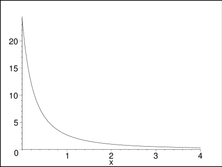
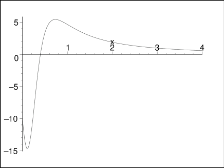
Figure 4: Reflectionless potentials $V_{n}(x)$ and $V_{n+1}(x)$ for values $C_{1}=1$, $\gamma=6$ and $x_{0}=0.5$

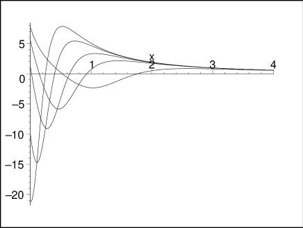
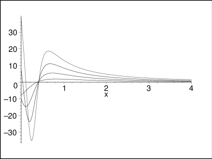
Figure 5: A dependence of the reflectionless potential $V_{n+1}(x)$ on the parameters $C_{1}$ and $\gamma$: at the change of the parameter $C_{1}$ the barrier maximum and the hole minimum of the potential is displaced along the axis $x$ (the first figure, the values $C_{1}=0.01,0.1,0.3,1.0,2.5$, $\gamma=6$, $x_{0}=0.5$), at the change of the parameter $\gamma$ the barrier maximum of the potential practically does not displaced along the axis $x$ (the second figure, values $C_{1}=1$, $\gamma=2,6,12,20$, $x_{0}=0.5$)

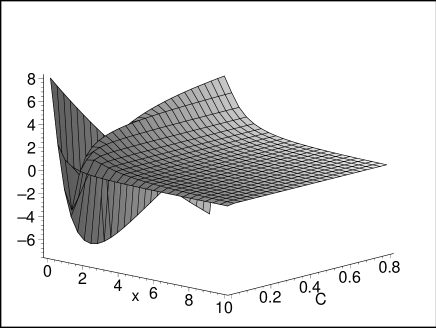
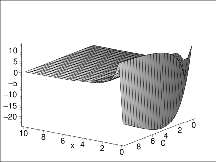
Figure 6: Continuous change of the form of the reflectionless potential $V_{n+1}(x)$ (with the barrier and the hole) at variation of the parameter $C_{1}$ ($\gamma=6$, $x_{0}=0.5$)

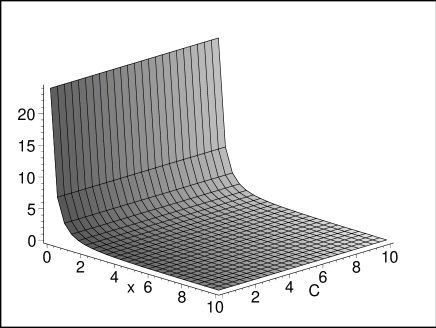
Figure 7: The reflectionless potential $V_{n+1}(x)$ does not changed at the change of the parameters $C_{1}$ and $\gamma$ (the diagrams coincide for different values $\gamma=2,6,12,20$, $x_{0}=0.5$)

Let’s analyze the change of the form of the potentials $V_{n}(x)$ and $V_{n+1}(x)$ in variation of the parameters $C_{1}$ and $\gamma$ in the case $2\beta\neq\alpha$. Diagrams of these potentials for values $C_{1}=1$ and $\gamma=6$ on the positive semi-axis $x\geq 0$ are shown in Fig. 4. From here one can see, that the potential $V_{n}(x)$ remains inverse power, but a barrier and a hole appear in the potential $V_{n+1}(x)$. This second potential is qualitatively similar to a radial interaction potential in the elastic scattering of particles on nuclei and in decay of compound nuclei in the spherically symmetric consideration. Such a form of the reflectionless potential and its application to the scattering theory are found for the first time. From Fig. 5 one can see, that locations of the barrier maximum and the hole minimum of the potential $V_{n+1}(x)$ are shifted along the axis $x$ at the change of the parameter $C_{1}$, but the change of the parameter $\gamma$ practically does not influence on the location of the barrier maximum of this potential. In Fig. 6 we show the continuous change of the form of this potential at the change of the parameter $C_{1}$ (here one can see, how the barrier and hole are changed). In accordance with preliminary calculations, the change of the parameters does not influence on the form of the potential $V_{n}(x)$ (see Fig. 7).

From (86) one can see, that at $C_{1}\to 0$ (at $2\beta\neq\alpha$) the superpotential tends to the earlier known function (50) with taking into account of (51). But at $C_{1}\neq 0$ we obtain new reflectionless potentials (and the superpotentials, corresponding to them).

5.3.3 Scaling of the reflectionless potential

If we know the reflectionless potential $V_{n}(x)$, then the potential $V_{n+1}(x)=CV_{n}(x)$ (where $C=const$) is also reflectionless. Really, let $V_{n}(x)$ is the reflectionless potential. Then we write:

$$\begin{array}[]{c}-\displaystyle\frac{\hbar^{2}}{2m}\displaystyle\frac{d^{2}}{dx^{2}}\varphi^{(n)}(x)+(V_{n}(x)-E^{(n)})\varphi^{(n)}(x)=0,\\ V_{n+1}(x)=CV_{n}(x),\\ E^{(n+1)}=CE^{(n)}.\end{array}$$ (87)

From here we obtain the Schrödinger equation for the new potential:

$$\begin{array}[]{ll}-\displaystyle\frac{\hbar^{2}}{2m}\displaystyle\frac{d^{2}}{d\biggl{(}\displaystyle\frac{x}{\sqrt{C}}\biggr{)}^{2}}\varphi^{(n)}(x)+(V_{n+1}(x)-E^{(n+1)})\varphi^{(n)}(x)=0.&\end{array}$$ (88)

Conclusion: if $V_{n}(x)$ is a reflectionless potential, then $V_{n+1}(x)=CV_{n}(x)$ is also the reflectionless potential having the energy spectrum $E^{(n+1)}$, compressed relatively $E^{(n)}$, and the wave function $\varphi^{(n+1)}(x)$, compressed along the axis $x$ relatively the wave function $\varphi^{(n)}(x)$:

$$\begin{array}[]{ll}E^{(n+1)}=CE^{(n)},&\varphi^{(n+1)}(x)=\varphi^{(n)}\biggl{(}\displaystyle\frac{x}{\sqrt{C}}\biggr{)}.\end{array}$$ (89)

5.3.4 Spatial symmetry of the reflectionless potentials

Let’s analyze, whether the reflectionless potentials have a property of the spatial symmetry or antisymmetry at change $x\to-x$. At first we shall consider the potentials-partners to the constant potential (20) with the number “up” and the superpotentials, corresponding to them, in the case $x_{0}\to 0$ (i. e. at the exception of the parameter $x_{0}$). From the general form of the solutions from the second up to the fifth one of the superpotential (33) and the potential-partners (34) one can conclude:

$$\begin{array}[]{ll}W_{n+1}(-x)=-W_{n+1}(x),&\mbox{for }|W(x)|\neq|A|,x\neq 0\mbox{ and }x_{0}=0;\\ V_{n+1}(-x)=V_{n+1}(x),&\mbox{for }|W(x)|\neq|A|,x\neq 0\mbox{ and }x_{0}=0;.\end{array}$$ (90)

This property is fulfilled for the superpotential and the potential-partner to the constant potential with the number “down” (see (37) and (38)). Therefore, any potential-partner to the constant potential is spatially symmetric at $x_{0}\to 0$ (i. e. it keeps a sign at the change $x\to-x$), and the superpotential, connected to it, spatially antisymmetric (i. e. it changes a sign at the change $x\to-x$).

Let we know a general form of the superpotential $W_{n}(x)$ with the number $n$, which is antisymmetric function. According to (77), there is a partial solution for the superpotential with the number $n+1$, which also is antisymmetric function. In order to analyze, whether there a general solution for the superpotential $W_{n}(x)$ is the antisymmetric function, we shall consider the expression (85). The integral $\int\exp{(2\tilde{W}(x)/\alpha)}\,dx$ is the indefinite integral from the antisymmetric function and, therefore, it is the symmetric function. Then the function $W(x)$ defined by (85), is the antisymmetric function at $C_{1}=0$ also.

Thus, we have proved the following property: any reflectionless potential, which belongs to SUSY-hierarchy with the constant potential, and is defined with all parameters (the constant of integration), which are equal to zero, is spatially symmetric, and the superpotential, concerned with it, is spatially antisymmetric.

If one of free parameters is distinct from zero, then the spatial symmetry of the potential can be broken, that will result in occurrence of new spatially asymmetric reflectionless potentials (it is found for the first time). One can use this idea for construction of new reflectionless spatially asymmetrical potentials (in specific case, which are defined by one continuous function on the whole axis $x$). Generally, the potential of the reflectionless SUSY-hierarchy can not be antisymmetric function (and any of all superpotentials connecting it with the constant potential in this SUSY-hierarchy, can not be symmetric function, with the exception for constant).

It will be interesting to apply this analysis for the known reflectionless soliton-like potentials, reflectionless one and many-steps shape invariant potentials (with different types of parameter transformations), and reflectionless potentials found on the basis of methods of inverse problem.

6 Conclusions

In this paper the class of the one-dimensional reflectionless potentials constituted into one SUSY-hierarchy is studied. Note the following conclusions.

• The new approach for determination of the general form of the reflectionless potential on the basis of construction of the SUSY-hierarchy, which contains the constant potential, and extraction from it the potentials, which are finite on the whole axis $x$ and in the asymptotic areas tend to uniquely finite limits, is proposed.

• The assumption about that a reason of the absolute transparency of any reflectionless potential consists in its SUSY-interrelation with the constant potential, is putted.

• The general integrated form of the interdependence between the superpotentials with neighboring numbers in the SUSY-hierarchy of the reflectionless potentials (in analytical solution of the Ricatti equation) is found.

• The way of construction of the new reflectionless potentials of a simple analytical form, which are expressed through finite number of the elementary functions on the basis of the obtained above interdependence between the superpotentials, is pointed out.

• It is shown, that the constant potential has only five different types of its SUSY potentials-partners expressed through the elementary functions, from which the reflectionless potentials can be selected.

• The analysis of existence of an absolute transparency for the potential having the inverse power dependence on spatial coordinate (and where tunneling is possible), i. e. of the form $V(x)=\pm\alpha/|x-x_{0}|^{n}$ (where $\alpha$ and $x_{0}$ are constant, $n$ is natural number), is fulfilled. It is shown, that such potential can be reflectionless at $n=2$ only. The SUSY-hierarchy of the inverse power reflectionless potentials is constructed.

• The assumption about that any reflectionless potential can be presented in an integrated form (or in a simple analytical form) with use of the finite number of the elementary functions (in particular, such a representation can exist for the known reflectionless soliton-like potentials or the known shape invariant potentials with one or many steps scaling of parameter, which are expressed through series), is formulated.

• The new types of the reflectionless potentials of a simple analytical form, which look (on the semi-axis $x$) like the radial interaction potential with the barrier and the hole between particles with nuclei at their elastic scattering (or for decay of the compound spherical systems), are opened. Such potentials can present new exactly solvable models.

• The new way of construction of the spatially asymmetrical reflectionless potentials (relatively a point $x=0$) is pointed out.

Perspectives of such representations of the reflectionless potentials consist in their simple analytical form, that is convenient at a qualitative analysis of properties of tunneling processes.

References

- (1) V. M. Chabanov and B. N. Zakhariev, Absolutely transparent multichannel systems. Unexpected peculiarities, Physics Letters B 319 (1–3), (1993) 13–15.
- (2) N. Saito and Y. Kayanuma, Resonant tunneling of a composite particle through a single potential barrier, Journal of Physics: Condensed Matter 6 (1994) 3759–3766.
- (3) K. Chadan, P. C. Sabatier, Inverse problems in quantum scattering theory, Springer-verlag, New York, 1977, p. 377.
- (4) B. N. Zakhariev and V. M. Chabanov, Qualitative theory of control of spectra, scattering, decays (Quantum intuition lessons), Physics of elementary particles and atomic nuclei 25 (Iss. 6), (1994) 1561–1597 — [in Russian].
- (5) B. N. Zakhariev and V. M. Chabanov, On the qualitative theory of elementary transformations of one- and multicannel quantum systems in the inverse problem approach, Physics of elementary particles and atomic nuclei 30 (Iss. 2), (1999) 277–320 — [in Russian].
- (6) A. Khare and U. P. Sukhatme, New shape invariant potentials in supersymmetric quantum mechanics, Journal of Physics A: General 26 (1993) L901–L904; hep-th/9212147.
- (7) A. B. Balantekin, Algebraic approach to shape invariance, Physical Review A57 (1998) 4188–4191; quant-ph/9712018.
- (8) A. Shabat, Inverse Problems 8 (1992) 303.
- (9) V. Spiridonov, Physical Review Letters 69 (1992) 398.
- (10) D. T. Barclay, R. Dutt, A. Gangopadhyaya, A. Khare, A. Pagnamenta and U. Sukhatme, New exactly solvable Hamiltonians: shape invariance and self-similarity, Physical Review A48 (1993) 2786–2797; hep-ph/9304313.
- (11) V. Spiridonov, Modern Physics Letters 7 (1992) 1241.
- (12) F. Cooper, A. Khare and U. Sukhatme, Supersymmetry and quantum mechanics, Physics Reports 251 (1995) 267–385; hep-th/9405029.
- (13) B. N. Zakhariev, A. A. Suzko, Potentsiali i kvantovoe rasseyanie: pryamaya i obratnaya zadachi, Energoatomizdat, Moskva, 1985, p. 224 — [in Russian].
- (14) S. P. Maydanyuk, One-dimensional inverse power reflectionless potentials (talk on the II Conference on High Energy Physics, Nuclear Physics and Accelerator Physics, March 1-5, 2004, Kharkov, Ukraine), Problems of atomic science and technology. Series: Nuclear Physics Investigations (44) 5, 22-25, 2004; quant-ph/0404021.
- (15) A. N. Tihonov, A. B. Vasilieva, A. G. Sveshnikov, Differentsialnie uravneniya, Nauka – Fizmatlit, Moskva, 1998, p. 232 — [in Russian].