We propose a new, twistor string theory inspired formalism to calculate loop amplitudes in ${\cal N}=4$ super Yang-Mills theory. In this approach, maximal helicity violating (MHV) tree amplitudes of ${\cal N}=4$ super Yang-Mills are used as vertices, using an off-shell prescription introduced by Cachazo, Svrcek and Witten, and combined into effective diagrams that incorporate large numbers of conventional Feynman diagrams. As an example, we apply this formalism to the particular class of supersymmetric MHV one-loop scattering amplitudes with an arbitrary number of external legs in ${\cal N}=4$ super Yang-Mills. Remarkably, our approach naturally leads to a representation of the amplitudes as dispersion integrals, which we evaluate exactly. This yields a new, simplified form for the MHV amplitudes, which is equivalent to the expressions obtained previously by Bern, Dixon, Dunbar and Kosower using the cut-constructibility approach.

1 Introduction

It has been proposed recently [1] that ${\cal N}=4$ super Yang-Mills (SYM) has a formulation as a topological string theory in super twistor space. This proposal, and related formulations, have since been actively investigated (see [1]–​​[25]). The original maximal helicity violating (MHV) tree amplitudes given in [26, 27] take a surprisingly simple form, and the tree amplitudes in the gauge theory have now been understood in the context of this topological string theory. Inspired by the twistor approach, the MHV amplitudes were used as vertices by Cachazo, Svrcek and Witten (CSW) in [6], together with a particular off-shell prescription, in order to present a new and extremely efficient method of deriving more general, non-MHV tree amplitudes. This has been further explored in [7, 13, 20, 22, 21, 23, 24]. The CSW method of constructing gauge theory tree amplitudes corresponds in the twistor picture to completely disconnected instantons of degree one, linked by twistor space propagators, whereas the original approach of [1] used connected higher degree instantons. The picture emerging is that there appears to be a number of alternative ways to compute tree amplitudes, which are related by the degeneration of higher degree curves into curves of lower degree [2, 4, 10, 14, 21].

The study of quantum amplitudes in ${\cal N}=4$ SYM has led to many interesting results - see [28]–​​[38] and references therein. Much of this progress was achieved thanks to powerful unitarity-based methods [30, 34, 33, 31, 38], whereby properties of loop amplitudes are derived from cutting rules and tree amplitudes. One of the main virtues of this approach lies in the fact that the tree amplitudes on both sides of the cut are evaluated on-shell, and can moreover be simplified before constructing the loop amplitude. This is referred to as the “cut-constructibility” approach. The simplest application concerns the calculation of one-loop MHV diagrams (see [32, 33] for reviews). Here one can derive explicit expressions for the amplitudes at one loop using the known results for the tree-level MHV amplitudes [29]. Recent work [36, 37] has also uncovered intriguing recursion relations which link two-loop amplitudes to those at one loop, and led to speculation about the existence of more general cross-order relations between $L-1$ and $L$ loop amplitudes.

So far, twistor-inspired techniques have successfully reproduced known MHV and non-MHV tree amplitudes and inspired efficient new techniques to calculate new tree amplitudes. One expects that this success will carry over to perturbative calculations at the loop level. Whilst some initial comments on loop diagrams were already made in [1] and, more recently, the twistor space structure of one-loop diagrams in ${\cal N}=4$ SYM has been analysed in [25], it has so far not been clear how to relate loop amplitudes directly to string theory in twistor space. Indeed, in the presently known twistor string theories, conformal supergravity does not decouple from the gauge theory, which implies that also supergravity fields can propagate in loops and the twistor/gauge theory correspondence is spoiled at the loop level [19].

However, even without the knowledge of the correct twistor string theory description, one can investigate the calculation of loop amplitudes, using recent results. Firstly, the recently obtained formulae for tree amplitudes can be fed into the known field theoretical unitarity-based methods; and secondly, one can attempt, using twistor intuition, to find new field theory prescriptions to compute scattering amplitudes. An example of the latter is the off-shell prescription of CSW [6], that uses MHV amplitudes continued off-shell as vertices for constructing more general non-MHV amplitudes at the tree level. It is natural to try to apply this to the computation of loop diagrams, in particular to the simplest case of the supersymmetric one-loop MHV amplitudes, where one can link to known results. This will be the subject of this paper.

Specifically, we will find that twistor-inspired techniques, when applied to one-loop diagrams, naturally generate dispersion integrals, in terms of which the amplitudes are described. We find that our expression for the MHV scattering amplitudes is in exact agreement with the result for this class of amplitudes obtained previously by Bern, Dixon, Dunbar and Kosower (BDDK) [29] using the cut-constructibility approach.

The evaluation of the dispersion integrals proves, rather surprisingly, to be tractable, and provides a simpler formulation of the amplitudes in terms of a new form for the so-called “two easy masses” box function - see (7). We expect this to be an important ingredient in further work, both in the calculation of other loop amplitudes, and in the development of the twistor space picture. The appearance of dispersion integrals in this construction is rather striking. Does twistor string theory presage the return of the analytic S-matrix?

The rest of the paper is organised as follows. In Section 2 we briefly review the unitarity-based cut-constructibility approach used by BDDK in [29] in order to derive formulae for the one-loop MHV amplitudes. In Section 3 we explain how MHV tree amplitudes, continued off-shell using a prescription equivalent to that of [6], lift to effective vertices and can be used to build loop diagrams which are made of collections of MHV vertices connected by scalar propagators. Loop amplitudes are then obtained by summing over appropriate MHV Feynman diagrams. In Section 4 we calculate supersymmetric MHV amplitudes at one loop using the procedure outlined in Section 3. Specifically, we will combine the off-shell MHV vertices into one-loop diagrams, and show that this approach yields dispersion integrals which reproduce the known results for MHV one-loop amplitudes (expressed in terms of scalar box integrals). The formal proof of this is presented in Section 4. Section 5 is devoted to the explicit calculations of the corresponding dispersion integrals, for the case of the $n$-particle MHV scattering amplitude. We find a new formulation of the box functions appearing in the amplitude, and show that this agrees with the known expressions for the MHV amplitudes at one loop, using a nine dilogarithm identity proved in an Appendix. In Section 6 we briefly comment on vanishing one-loop amplitudes. Finally, we present our conclusions in Section 7.

2 One-loop MHV amplitudes from unitarity

In this section we will briefly review the derivation of BDDK for the one-loop MHV ${\cal N}=4$ super Yang-Mills amplitudes from unitarity constraints, given in [29]. We refer the reader to this reference for more details. We suppress constant factors connected with dimensional regularisation where they are not essential to the discussion.

The full one-loop $n$-point MHV amplitudes in ${\cal N}=4$ super Yang-Mills are proportional to the tree level amplitudes,

$$A_{n;1}^{{\cal N}=4\,{\rm MHV}}=A^{\rm tree}_{n}\,V_{n}^{g}.$$ (2.1)

The function $V_{n}^{g}$ is given in terms of scalar box functions $F$ by

$$V^{g}_{2m+1} = \sum_{r=2}^{m-1}\sum_{i=1}^{n}F_{n:r;i}^{2m\,e}+\sum_{i=1}^{n}F_{n:i}^{1m}\ ,$$

$$V^{g}_{2m} = \sum_{r=2}^{m-2}\sum_{i=1}^{n}F_{n:r;i}^{2m\,e}+\sum_{i=1}^{n}F_{n:i}^{1m}+\sum_{i=1}^{n/2}F_{n:m-1;i}^{2m\,e}\ ,$$ (2.2)

or, more compactly [25],

$$V^{g}_{n} = \sum_{i=1}^{n}\sum_{r=1}^{[{n\over 2}]-1}\Bigl{(}1-{1\over 2}\delta_{{n\over 2}-1,r}\Bigr{)}\,F_{n:r;i}^{2m\,e}\ .$$ (2.3)

The basic scalar box integral $I_{4}$ is defined by

$$I_{4}=-i(4\pi)^{2-\epsilon}\,\int\frac{d^{4-2\epsilon}p}{(2\pi)^{4-2\epsilon}}\,\,\frac{1}{p^{2}(p-K_{1})^{2}(p-K_{1}-K_{2})^{2}(p+K_{4})^{2}}\ ,$$ (2.4)

where dimensional regularisation is used in order to take care of infrared divergences. The relevant integrals arising in the one-loop MHV diagrams are related to $I_{4}$ for certain choices of momenta $K$, and are denoted by $I_{4:i}^{1m}$ and $I_{4:r;i}^{2m\,e}$. These are given in terms of the $F$ functions in (2) by

$$I_{4:i}^{1m} = \frac{-2F_{n:i}^{1m}}{t^{[2]}_{i-3}t^{[2]}_{i-2}}\ ,$$

$$I_{4:r;i}^{2m\,e} = \frac{-2F_{n:r;i}^{2m\,e}}{t^{[r+1]}_{i-1}t^{[r+1]}_{i}-t^{[r]}_{i}t^{[n-r-2]}_{i+r+1}}\ ,$$ (2.5)

with

$$t_{i}^{[r]}=(k_{i}+\dots+k_{i+r-1})^{2}$$ (2.6)

(the $k_{i}$ are the external momenta). The $F$ functions depend on the variables $t_{i}^{[r]}$ for certain values of $i,r$, and involve logarithms and dilogarithms. Appendix I of [29] gives the explicit expressions.

It is also convenient to introduce the general scalar box function [25]

$$F(p,q,P,Q) := -{1\over\epsilon^{2}}\Bigl{[}\big{(}-(P+p)^{2}\bigr{)}^{-\epsilon}\,+\,\big{(}-(P+q)^{2}\bigr{)}^{-\epsilon}\,-\,\big{(}(-P)^{2}\bigr{)}^{-\epsilon}\,-\,\big{(}(-Q)^{2}\bigr{)}^{-\epsilon}\Bigr{]}$$ (2.7)

$$+ {\rm Li}_{2}\Bigl{(}1-{P^{2}\over(P+p)^{2}}\Bigr{)}\,+\,{\rm Li}_{2}\Bigl{(}1-{P^{2}\over(P+q)^{2}}\Bigr{)}$$

$$+ {\rm Li}_{2}\Bigl{(}1-{Q^{2}\over(Q+q)^{2}}\Bigr{)}\,+\,{\rm Li}_{2}\Bigl{(}1-{Q^{2}\over(Q+p)^{2}}\Bigr{)}$$

$$- {\rm Li}_{2}\Bigl{(}1-{P^{2}Q^{2}\over(P+p)^{2}(P+q)^{2}}\Bigr{)}\,+\,{1\over 2}\log^{2}\Bigl{(}{(P+p)^{2}\over(P+q)^{2}}\Bigr{)}\ ,$$

where $P+p+Q+q=0$. Introducing the convenient variables

$$s\ :=\ (P+p)^{2}\ ,\qquad t\ :=\ (P+q)^{2}\ ,$$ (2.8)

we can rewrite (2.7) as

$$F(s,t,P^{2},Q^{2}) := -{1\over\epsilon^{2}}\Bigl{[}(-s)^{-\epsilon}\,+\,(-t)^{-\epsilon}\,-\,\big{(}(-P)^{2}\bigr{)}^{-\epsilon}\,-\,\big{(}(-Q)^{2}\bigr{)}^{-\epsilon}\Bigr{]}$$ (2.9)

$$+ {\rm Li}_{2}\Bigl{(}1-{P^{2}\over s}\Bigr{)}\,+\,{\rm Li}_{2}\Bigl{(}1-{P^{2}\over t}\Bigr{)}+{\rm Li}_{2}\Bigl{(}1-{Q^{2}\over s}\Bigr{)}\,+\,{\rm Li}_{2}\Bigl{(}1-{Q^{2}\over t}\Bigr{)}$$

$$- {\rm Li}_{2}\Bigl{(}1-{P^{2}Q^{2}\over s\,t}\Bigr{)}\,+\,{1\over 2}\log^{2}\Bigl{(}{s\over t}\Bigr{)}\ .$$

The relation to the functions $F_{n:r;i}^{2m\,e}$ is obtained by setting $p=p_{i-1}$, $q=p_{i+r}$, and $P=p_{i}+\cdots+p_{i+r-1}$. In the following sections we will make use of the discontinuities of the function $F$ across its branch cuts. A derivation of these discontinuities up to ${\cal O}(\epsilon^{0})$ can be found in Appendix A and, up to and including ${\cal O}(\epsilon)$ terms, in Appendix B, where these discontinuities are evaluated from phase space integrals.

The one-loop MHV amplitudes were constructed in [29] from tree diagrams using cuts. A given cut results in singularities in the relevant momentum channels, and from considering all possible cuts one can construct the full set of possible singularities. From this and unitarity one can deduce the amplitude as given in (2.1). More explicitly, consider a cut one-loop MHV diagram where the cut separates the external momenta $k_{{m_{1}}}$ and $k_{{m_{1}}-1}$, and $k_{{m_{2}}}$ and $k_{{m_{2}}+1}$ (i.e. the set of external momenta $k_{{m_{1}}},k_{{m_{1}}+1},...,k_{{m_{2}}}$ lie to the left of the cut, and the set $k_{{m_{2}}+1},k_{{m_{2}}+2},...,k_{{m_{1}}-1}$ lie to the right, with momenta labelled clockwise and outgoing). This separates the diagram into two MHV tree diagrams connected only by two momenta $l_{1}$ and $l_{2}$ flowing across the cut, with

$$l_{1}=l_{2}+P_{L}\ ,$$ (2.10)

where $P_{L}=\sum_{i={m_{1}}}^{{m_{2}}}k_{i}$ is the sum of the external momenta on the left of the cut. The momenta $l_{1},l_{2}$ are taken to be null. It is important to note that the resulting integrals are not equal to the corresponding Feynman integrals where $l_{1}$ and $l_{2}$ would be left off shell; however, the discontinuities in the channel under consideration are identical and this gives enough information to determine the full amplitude uniquely.

It is immediate to see that the integrand which arises from the cut diagram involves the function [29]

$$\hat{{\cal R}}\ :=\ {\langle m_{1}-1\,m_{1}\rangle\langle l_{2}\,l_{1}\rangle\over\langle m_{1}-1\,l_{1}\rangle\langle-l_{1}\,m_{1}\rangle}\ {\langle m_{2}\,m_{2}+1\rangle\langle l_{1}\,l_{2}\rangle\over\langle m_{2}\,l_{2}\rangle\langle-l_{2}\,m_{2}+1\rangle}\ .$$ (2.11)

With the help of the Schouten identity we are able to rewrite

$$\langle m_{1}-1\,m_{1}\rangle\langle l_{2}\,l_{1}\rangle = \langle m_{1}-1\,l_{1}\rangle\langle l_{2}\,m_{1}\rangle\,+\,\langle m_{1}-1\,l_{2}\rangle\langle m_{1}\,l_{1}\rangle\ ,$$ (2.12)

$$\langle m_{2}\,m_{2}+1\rangle\langle l_{1}\,l_{2}\rangle = \langle m_{2}\,l_{2}\rangle\langle l_{1}\,m_{2}+1\rangle\,+\,\langle m_{2}\,l_{1}\rangle\langle m_{2}+1\,l_{2}\rangle\ ,$$

and hence

$$\hat{{\cal R}}={\cal R}(m_{1},m_{2}+1)+{\cal R}(m_{1}-1,m_{2})-{\cal R}(m_{1},m_{2})-{\cal R}(m_{1}-1,m_{2}+1)\ ,$$ (2.13)

where we define ${\cal R}(i,j)$ to be the homogeneous function of the spinors $l_{1}$ and $l_{2}$ given by

$${\cal R}(i\,j)\,:=\,{\langle i\,l_{2}\rangle\over\langle i\,l_{1}\rangle}\,{\langle j\,l_{1}\rangle\over\langle j\,l_{2}\rangle}\ .$$ (2.14)

We now rewrite the integrand in terms of the scalar functions appearing in the bubble, triangle and box integrals. Firstly, we notice that

$${\cal R}(i\,j)\, = {\langle i\,l_{2}\rangle\,[l_{2}\,j]\,\langle j\,l_{1}\rangle\,[l_{1}\,i]\over\langle i\,l_{1}\rangle\,[l_{1}\,i]\,\langle j\,l_{2}\rangle\,[l_{2}\,j]}\ =\ {{\rm Tr}\left[{1\over 2}(1+\gamma^{5})\,\hat{l}_{1}\,\hat{i}\,\hat{l}_{2}\,\hat{j}\right]\over(l_{1}-i)^{2}(l_{2}+j)^{2}}$$

$$= {2\left[(l_{1}\,i)(l_{2}\,j)+(l_{1}\,j)(l_{2}\,i)-(l_{1}\,l_{2})(i\,j)\right]\over(l_{1}-i)^{2}(l_{2}+j)^{2}}\ .$$

Of course, one could equally write $\langle l_{1}\,i\rangle\,[l_{1}\,i]=2(li)=(l_{1}+i)^{2}=-(l_{1}-i)^{2}$ for example. The correct choice of the signs in the denominator in (2) is made according to the momentum flow. In (2) and in the following paragraph we have written the signs which are appropriate for $i=m_{1}$, $j=m_{2}$. The other possible cases, corresponding to the possible arguments of the ${\cal R}$ functions on the right hand side of (2.13), are treated in a similar manner.

The next step consists in using (2.10) to rewrite the second and last terms in the numerator of the last expression in (2). The cancellation of bubble and triangle integrals then takes place upon summing over the four terms in (2.13). One may anticipate this cancellation by defining an effective function ${\cal R}^{\rm eff}(i,j)$ - this is defined to be ${\cal R}(i\,j)$ minus the terms which cancel upon the summation involved in (2.13). One finds that

$${\cal R}^{\rm eff}(i,j)=\frac{-2(P_{L}\,i)(P_{L}\,j)+P_{L}^{2}(i\,j)}{(l_{1}-i)^{2}(l_{2}+j)^{2}}\ ,$$ (2.16)

and one may use this to define a function ${\cal R}^{\rm eff}$ in an analogous way to (2.13).

Now note the identity

$$4(Pi)(Pj)-2P^{2}(ij)=(P+i)^{2}(P+j)^{2}-P^{2}(P+i+j)^{2}\ ,$$ (2.17)

for any momentum $P$, where $i,j$ refer to null momenta. In other words, the left hand side of (2.17) is invariant under

$$P\to P+ai+bj\ ,$$ (2.18)

where $a$ and $b$ are arbitrary numbers. Using this, one can show that the momentum dependence from the numerator in (2.16) precisely cancels that from the denominator in the definition of the functions $I$ in (2) in each of the four cases which arise in ${\cal R}^{\rm eff}$. One is finally left with the result that the cut diagram considered gives rise to the sum of four discontinuities (in the same channel) of four different $F$ functions (three when a cut leaves only two legs on one side), one for each of the cut box diagrams which arise . The knowledge of all cuts, together with the fact that due to general arguments [29] this class of amplitudes is given by a sum of scalar box integrals $F$, is sufficient to fix the full amplitude uniquely, and it is simply given by (2) as a sum over all scalar box functions $F$ with all coefficients equal to $1$.

3 Off-shell derivation of the one-loop amplitudes

The procedure summarized above for calculating the one-loop MHV amplitude involved the study of all possible cuts. The calculation of cuts involves an integration over the Lorentz invariant phase space (LIPS) measure, which puts the momenta $l_{1},l_{2}$ crossing the cut on-shell. This fact allows one to insert the tree MHV amplitudes directly into the integrals of the cuts, and was also crucial in various algebraic manipulations which led to cancellations and the simplicity of the final expression.

In [6] a prescription for taking momenta of external lines in MHV-amplitudes off shell was given, and used to combine tree MHV diagrams in such a way as to produce non-MHV tree amplitudes. In this section we will define an off-shell prescription that can be applied to one-loop diagrams (and we expect also to higher-loop diagrams). In Sections 4 and 5 we will show that combining MHV vertices into one-loop diagrams using this off-shell prescription precisely yields the MHV results given earlier.

Consider an off-shell (loop) vector $L$. It can be decomposed as [21, 23]

$$L\ =\ l\,+\,z\eta\ ,$$ (3.1)

where $l^{2}=0$, and $\eta$ is a fixed (and arbitrary) null vector, $\eta^{2}=0$; $z$ is a real number. Equation (3.1) determines $z$ as a function of $L$ to be

$$z\ =\ {L^{2}\over 2(L\eta)}\ .$$ (3.2)

Notice that $L^{2}=z(l+\eta)^{2}$; since the null vector $l$ has a non-negative energy component and $\eta$ is null as well, it follows that $(l+\eta)^{2}$ has a definite sign unless the two vectors are proportional. This implies that the sign of $L^{2}$ is directly related to the sign of $z$.

We can write the null vectors $l$ and $\eta$ in terms of spinors as $l_{\alpha{\dot{\alpha}}}=l_{\alpha}\tilde{l}_{{\dot{\alpha}}}$, $\eta_{\alpha{\dot{\alpha}}}=\eta_{\alpha}\tilde{\eta}_{{\dot{\alpha}}}$, from which it follows that

$$l_{\alpha} = {L_{\alpha{\dot{\alpha}}}\tilde{\eta}^{{\dot{\alpha}}}\over[\tilde{l}\,\tilde{\eta}]}\ ,$$ (3.3)

$$\tilde{l}_{{\dot{\alpha}}} = {\eta^{\alpha}L_{\alpha{\dot{\alpha}}}\over\langle l\,\eta\rangle}\ .$$ (3.4)

These equations coincide with the CSW prescription [6] for determining the spinor variables $l$ and $\tilde{l}$ associated with the off-shell (i.e. non-null) four-vector $L$ defined in (3.1). The denominators on the right hand sides of (3.3) and (3.4) will be irrelevant for our applications, since the expressions we will be dealing with are homogeneous in the spinor variables $\eta$; we will discard them.

In order to calculate loop diagrams, we need to re-express the integration measure $d^{4}L$ (which appears in the expression of loop integrals) in terms of the new variables $l$ and $z$ introduced previously. For our purposes it is useful to consider the product of the momentum measure and a massless scalar propagator. After a short calculation, one finds that

$${d^{4}L\over L^{2}}\ =\ d{\cal N}(l)\,{dz\over z}\ ,$$ (3.5)

where we have introduced the Nair measure [40]

$$d{\cal N}(l):=\,\langle l\,\,dl\rangle\,d^{2}\tilde{l}\ -\ [\tilde{l}\,\,d\tilde{l}]\,d^{2}l\ .$$ (3.6)

Importantly, the product of the measure factor with a scalar propagator $d^{4}L/L^{2}$ of (3.5) is independent of the reference vector $\eta$. The expression (3.5) will be central for our construction of loop diagrams.

Note that the Lorentz invariant phase space measure for a massless particle can be expressed precisely in terms of the Nair measure:

$$d^{4}l\,\delta^{(+)}(l^{2})\ =\ {d{\cal N}(l)\over 4i}\ ,$$ (3.7)

where, as before, we write the null vector $l$ as $l_{\alpha{\dot{\alpha}}}=l_{\alpha}\tilde{l}_{{\dot{\alpha}}}$, and in Minkowski space we identify $\tilde{l}=l^{\ast}$.

We conclude this section by summarising the strategy that we will follow in order to evaluate a generic loop diagram.

The first step consists in building MHV Feynman diagrams out of MHV vertices. Each spinor variable of an MHV vertex corresponding to an internal line is taken off-shell using the prescription of CSW outlined in the beginning of this section. Internal lines are then connected by scalar off-shell propagators which connect particles of the same spin but opposite helicity. Note that each MHV vertex should be multiplied by an appropriate delta function for momentum conservation. In the next step we express all the loop integration momenta as in (3.1) and use the integration measure (3.5) which already incorporates the scalar off-shell propagators. Finally, one has to sum over all independent diagrams obtained in this fashion for a fixed ordering of external helicity states.

In Section 4 we carry out this programme for the particular case of MHV amplitudes at one loop. One of the features of this procedure is the fact that the integration measure is naturally expressed as the product of two terms:

• a Lorentz-invariant phase space measure, and

• an integration over the $z$-variables introduced according to (3.1) (one for each loop momentum).

The phase-space measure (a two-body phase space measure, at one loop) will be appropriately continued to $D=4-2\epsilon$ dimensions in order to deal with potential infrared divergences.

4 Supersymmetric MHV amplitudes at one loop from MHV vertices

We will now write down the expression for the one-loop supersymmetric MHV amplitude with $n$ external legs. In performing our analysis, we will make use of the supersymmetric formulation introduced in [40], which generalises the usual MHV amplitudes. In this setup, to each particle one associates the usual commuting spinors $\lambda_{\alpha}$, $\tilde{\lambda}_{{\dot{\alpha}}}$ (in terms of which the momentum of the $i$-th particle is $p_{\alpha{\dot{\alpha}}}^{i}=\lambda_{\alpha}^{i}\tilde{\lambda}_{{\dot{\alpha}}}^{i}$), as well as anticommuting variables $\eta_{A}^{i}$, where $A$ is an index of the anti-fundamental representation of $SU(4)$. The supersymmetric amplitude can then be expanded in powers of the various ${\cal N}=4$ superspace coordinates $\eta_{A}^{i}$, and each term of this expansion corresponds to a particular scattering amplitude in ${\cal N}=4$ SYM. A term containing $p$ powers of $\eta_{A}^{i}$ corresponds to a scattering process where the $i$-th particle has helicity $h_{i}=1-p/2$.

With this in mind, the expression for a supersymmetric $n$-valent MHV vertex is

$${\cal V}(1,\ldots,n)\ =\ i(2\pi)^{4}\delta^{(4)}\big{(}\sum_{i=1}^{n}\lambda^{i}\tilde{\lambda}^{i}\big{)}\,\delta^{(8)}\bigl{(}\sum_{i=1}^{n}\lambda^{i}\eta^{i}\bigr{)}\ \prod_{i=1}^{n}{1\over\langle i\,i+1\rangle}\ ,$$ (4.1)

where the spinors associated to off-shell legs are chosen according to the prescription (3.1) (or, equivalently, (3.3) and (3.4)).

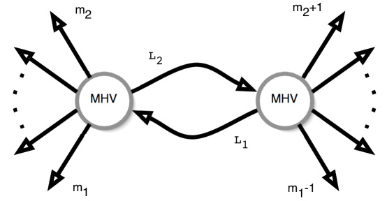
Figure 1: One-loop MHV Feynman diagram, computed in (4.2) using MHV amplitudes as interaction vertices, with the CSW off-shell prescription. The scattering amplitudes with the desired helicities for the external particles are then obtained by expanding the supersymmetric scattering amplitude in powers of the ${\cal N}=4$ coordinates $\eta^{i}$.

We can now write down the amplitude corresponding to the prototypical Feynman diagram we will consider, depicted in Figure 1. This is a diagram where the set of ordered external momenta $k_{1},\ldots,k_{n}$ is separated into two sets $k_{m_{1}},\ldots,k_{m_{2}}$ (on the left), and $k_{m_{2}+1},\ldots,k_{m_{1}-1}$ (on the right). Of course, the full one-loop MHV amplitude is obtained after summing over all the possible choices of these ordered sets. We will come back to this point later, as it is instructive to first discuss the structure of the generic one-loop diagram we want to compute.

The expression for the Feynman diagram in Figure 1 reads

$${\cal A}\ =\ i(2\pi)^{4}\delta^{(4)}(P_{L}+P_{R})\ \int\!{d^{4}L_{1}\over L_{1}^{2}}{d^{4}L_{2}\over L_{2}^{2}}\,\delta^{(4)}(L_{2}-L_{1}+P_{L})\,\int\!d^{8}\eta^{l_{1}}d^{8}\eta^{l_{2}}\,{\cal A}_{L}\,{\cal A}_{R}\ ,$$ (4.2)

where $P_{L}=\sum_{i=m_{1}}^{m_{2}}\lambda^{i}\tilde{\lambda}^{i}$ and $P_{R}=\sum_{j=m_{2}+1}^{m_{1}-1}\lambda^{j}\tilde{\lambda}^{j}$ are the sum of the momenta on the left and on the right of the diagram, respectively, and the tree amplitudes ${\cal A}_{L}$ and ${\cal A}_{R}$ are given by

$${\cal A}_{L} = \delta^{(8)}(\Theta_{L})\ {1\over\langle m_{2}\,l_{2}\rangle\langle-l_{1}\,m_{1}\rangle\langle l_{2}\,-l_{1}\rangle}\prod_{i=m_{1}}^{m_{2}-1}{1\over\langle i\,i+1\rangle}\ ,$$ (4.3)

$${\cal A}_{R} = \delta^{(8)}(\Theta_{R})\ {1\over\langle m_{1}-1\,l_{1}\rangle\langle-l_{2}\,m_{2}+1\rangle\langle l_{1}\,-l_{2}\rangle}\prod_{j=m_{2}+1}^{m_{1}-2}{1\over\langle j\,j+1\rangle}\ .$$

Here

$$(\Theta_{L})_{A\alpha} = \sum_{i\in L}\eta^{i}_{A}\lambda^{i}_{\alpha}\,+\,\eta_{A}^{l_{2}}l_{2\alpha}\,-\,\eta_{A}^{l_{1}}l_{1\alpha}\ ,$$ (4.4)

$$(\Theta_{R})_{A\alpha} = \sum_{j\in R}\eta^{j}_{A}\lambda^{j}_{\alpha}\,-\,\eta_{A}^{l_{2}}l_{2\alpha}\,+\,\eta_{A}^{l_{1}}l_{1\alpha}\ .$$

Notice that (4.2) is formally written in four dimensions, but should more correctly be analytically continued to $D=4-2\epsilon$ dimensions, due to the presence of infrared divergences. The effect of this is that the Lorentz invariant phase space measure in (4.11) below should be taken to be in $D=4-2\epsilon$ dimensions. For brevity we will still keep the four-dimensional notation.

Let us stress some important facts about (4.2).

• We have introduced off-shell vectors $L_{1}$ and $L_{2}$ as in (3.1), i.e.

  $$L_{i;\alpha,{\dot{\alpha}}}\ =\ l_{i\alpha}\tilde{l}_{i{\dot{\alpha}}}\,+\,z_{i}\,\eta_{\alpha}\tilde{\eta}_{{\dot{\alpha}}}\ ,\qquad i=1,2\ .$$ (4.5)

  These only appear in the measure factor $d^{4}L_{1}d^{4}L_{2}/(L_{1}^{2}L_{2}^{2})$, and in the delta function. Using (4.5), we will rewrite the argument of the delta function as

  $$L_{2}-L_{1}+P_{L}=l_{2}-l_{1}+P_{L;z}\ ,$$ (4.6)

  where we have defined

  $$P_{L;z}:=P_{L}-z\eta\ ,$$ (4.7)

  where

  $$z\ :=\ z_{1}\,-\,z_{2}\ .$$ (4.8)

  Note that we use the same $\eta$ for both the momenta $L_{i},i=1,2$.

• In the remaining part of the integrand we use, as spinors associated to the off-shell (loop) legs with momenta $L_{1}$ and $L_{2}$, precisely the spinors $l_{1\alpha}$ and $l_{2\alpha}$ of (4.5); this is the essence of the CSW prescription.

• We observe that

  $${d^{4}L_{1}\over L_{1}^{2}}{d^{4}L_{2}\over L_{2}^{2}}\,\delta^{(4)}(L_{2}-L_{1}+P_{L})\ =\ {dz_{1}\over z_{1}}\,{dz_{2}\over z_{2}}\ d{\cal N}(l_{1})\,d{\cal N}(l_{2})\ \delta^{(4)}(l_{2}-l_{1}+P_{L;z})$$

  (4.9)

  $$\ \ \ \ \ \ \ \ \ \ =\ -4\,{dz_{1}\over z_{1}}{dz_{2}\over z_{2}}\cdot\Big{[}d^{4}l_{1}\,\delta^{(+)}(l_{1}^{2})\ d^{4}l_{2}\,\delta^{(+)}(l_{2}^{2})\ \delta^{(4)}(l_{2}-l_{1}+P_{L;z})\Big{]}\ ,$$ (4.10)

  where we used (3.5) and (3.7). Note that the expression

  $$d{\rm LIPS}(l_{2},-l_{1};P_{L;z})\ :=\ d^{4}l_{1}\,\delta^{(+)}(l_{1}^{2})\ d^{4}l_{2}\,\delta^{(+)}(l_{2}^{2})\ \delta^{(4)}(l_{2}-l_{1}+P_{L;z})\ ,$$ (4.11)

  which appears in (3.), is nothing but the two-particle Lorentz invariant phase space measure. This will be crucial in the following. We can therefore rewrite (3.) as

  $${d^{4}L_{1}\over L_{1}^{2}}{d^{4}L_{2}\over L_{2}^{2}}\,\delta^{(4)}(L_{2}-L_{1}+P_{L})\ =\ -4\,{dz_{1}\over z_{1}}{dz_{2}\over z_{2}}\,d{\rm LIPS}(l_{2},-l_{1};P_{L;z})\ .$$ (4.12)

To deal with infrared divergences, we will dimensionally regularise the LIPS measure appearing in (4.12) to $D=4-2\epsilon$ dimensions.

Now we return to the evaluation of (4.2). We start off by integrating out the fermionic loop variables. This is easily accomplished by first writing

$$\delta^{(8)}(\Theta_{L})\delta^{(8)}(\Theta_{R})\ =\ \int\!d^{8}\theta d^{8}\theta^{{}^{\prime}}\ e^{i\theta_{a}^{A}(\Theta_{L})_{A}^{a}}\ e^{i\theta_{a}^{{}^{\prime}A}(\Theta_{R})_{A}^{a}}\ ,$$ (4.13)

where $\Theta_{L}$ and $\Theta_{R}$ are given in (4.4). Then

$$\int\!d^{4}\eta^{l_{1}}d^{4}\eta^{l_{2}}\ e^{i(\eta^{l_{1}}_{A}l_{1}^{\alpha}\,-\,\eta^{l_{2}}_{A}l_{2}^{\alpha})(\theta^{\prime}-\theta)_{\alpha}^{A}}\ =\ \langle l_{1}\,l_{2}\rangle^{4}\,\delta^{(8)}(\theta^{\prime}-\theta)\ .$$ (4.14)

In this way, (4.2) is recast as

$${\cal A}\ =\ {\cal A}_{\rm tree}\cdot{\cal L}\ ,$$ (4.15)

where the tree-level amplitude ${\cal A}_{\rm tree}$ is given by

$${\cal A}_{\rm tree}=i(2\pi)^{4}\delta^{(4)}(P_{L}+P_{R})\ \delta^{(8)}\big{(}\sum_{i=1}^{n}\eta^{i}_{A}\lambda^{i}_{\alpha}\big{)}\,\prod_{i=1}^{n}{1\over\langle i\,i+1\rangle}\ ,$$ (4.16)

and the integral ${\cal L}$ is

$${\cal L}\ =\ \int\!{d^{4}L_{1}\over L_{1}^{2}}{d^{4}L_{2}\over L_{2}^{2}}\delta^{(4)}(L_{2}-L_{1}+P_{L})\ {\langle m_{1}-1\,m_{1}\rangle\langle l_{2}\,l_{1}\rangle\over\langle m_{1}-1\,l_{1}\rangle\langle-l_{1}\,m_{1}\rangle}\ {\langle m_{2}\,m_{2}+1\rangle\langle l_{1}\,l_{2}\rangle\over\langle m_{2}\,l_{2}\rangle\langle-l_{2}\,m_{2}+1\rangle}\ .$$ (4.17)

We recognize in the integrand of (4.17) the function $\hat{{\cal R}}$ defined in (2.11).

We will now proceed to the evaluation of (4.17). Following steps similar to those of (2.11)–(2.16), we decompose $\hat{{\cal R}}$ as in (2.13) and we are left with a sum of four terms. Let us focus on the term $-{\cal R}(m_{1},m_{2})$ in (2.13); the other cases are treated analogously. This term generates a contribution to the amplitude which is proportional to

$${\cal I}=\int\!{d^{4}L_{1}\over L_{1}^{2}}{d^{4}L_{2}\over L_{2}^{2}}\delta^{(4)}(L_{2}-L_{1}+P_{L})\ {N(P_{z})\over(l_{1}-m_{1})^{2}\,(l_{2}+m_{2})^{2}}\ ,$$ (4.18)

that is

$${\cal I}=\int\!{dz_{1}\over z_{1}}\,{dz_{2}\over z_{2}}\ d{\cal N}(l_{1})\,d{\cal N}(l_{2})\ \delta^{(4)}(l_{2}-l_{1}+P_{L;z})\ {N(P_{z})\over(l_{1}-m_{1})^{2}\,(l_{2}+m_{2})^{2}}\ ,$$ (4.19)

where the numerator $N(P_{z})$ is defined by

$$N(P_{z}) := -2(P_{z}\cdot m_{1})(P_{z}\cdot m_{2})+P_{z}^{2}(m_{1}\cdot m_{2})$$ (4.20)

$$= -2(P_{L;z}\cdot m_{1})(P_{L;z}\cdot m_{2})+P_{L;z}^{2}(m_{1}\cdot m_{2})\ ,$$ (4.21)

and

$$P_{z} := \sum_{i=m_{1}+1}^{m_{2}-1}p_{i}-z\,\eta\ ,$$ (4.22)

$$P_{L;z} = P_{L}-z\eta=\sum_{i=m_{1}}^{m_{2}}p_{i}-z\,\eta\ =\ P_{z}\,+\,m_{1}\,+m_{2}\ .$$ (4.23)

$p_{i}=\lambda_{i}\tilde{\lambda}_{i}$ is the momentum of the $i$-th particle.

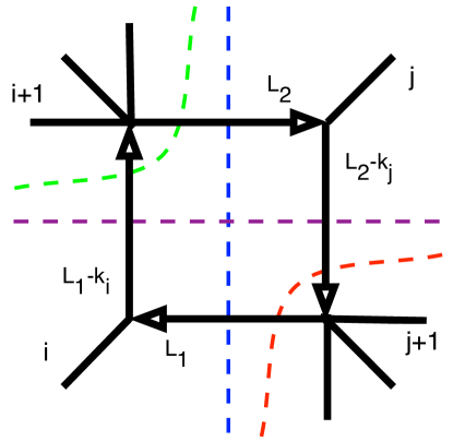
Figure 2: The possible cuts of a box diagram, corresponding to the function $F$ defined in (2.9). In the notation of that equation, $i$ and $j$ correspond to the momenta $p$ and $q$, respectively; and $P:=p_{i+1}+\cdots+p_{j-1}$, $Q:=p_{j+1}+\cdots+p_{i-1}$ correspond to the two groups of momenta on the upper left and lower right corner, respectively. The vertical (horizontal) cuts correspond to the $s$-channel ($t$-channel) cuts respectively, and the upper left (lower right) corner cuts to the $P^{2}$-channel ($Q^{2}$-channel) cuts respectively.

In the calculation reviewed in Section 2, where the MHV one-loop amplitude is reconstructed from the cuts, one was led to integrands involving the function defined in (2.16). More precisely, the numerator appearing in the corresponding box integral is the same as that in (4.20), but evaluated at $z=0$. Equivalently, our numerator (4.20) is related to that in the cut-constructibility picture simply by the shift

$$P_{L}\longrightarrow P_{L;z}=P_{L}-z\eta\ .$$ (4.24)

Next, we change variables from $(z_{1},z_{2})$ to $(z,z^{\prime})$, where $z^{\prime}=z_{1}+z_{2}$, so that

$${\cal I}\ =2\int\!{dz\,dz^{\prime}\over(z^{\prime}+z)\,(z^{\prime}-z)}\ d{\cal N}(l_{1})\,d{\cal N}(l_{2})\ \delta^{(4)}(l_{2}-l_{1}+P_{L;z})\ {N(P_{L;z})\over(l_{1}-m_{1})^{2}\,(l_{2}+m_{2})^{2}}\ ,$$ (4.25)

and perform the integration over $z^{\prime}$. Equation (4.25) turns into

$${\cal I}\ = 2(2\pi i)\int\!{dz\over z}\ d{\cal N}(l_{1})\,d{\cal N}(l_{2})\ \delta^{(4)}(l_{2}-l_{1}+P_{L;z})\ {N(P_{L;z})\over(l_{1}-m_{1})^{2}\,(l_{2}+m_{2})^{2}}$$ (4.26)

$$= -8(2\pi i)\int\!{dz\over z}\,d{\rm LIPS}(l_{2},-l_{1};P_{L;z})\ {N(P_{L;z})\over(l_{1}-m_{1})^{2}\,(l_{2}+m_{2})^{2}}\ .$$

In the last step we have used the two-particle Lorentz-invariant phase space measure from (4.11).

Let us briefly comment on the appearance of the LIPS measure in (4.26) and its consequences. This is the point where the off-shell calculation presented in this paper makes contact with the approach of BDDK, where one-loop amplitudes are reconstructed from the evaluation of the cuts in the various channels. Indeed, the LIPS measure is precisely what is required by Cutkosky’s cutting rules [41] to compute the discontinuity of a Feynman diagram across the branch cuts. Which discontinuity is evaluated is determined by the argument in the delta function appearing in the LIPS measure; in the case of (4.26), this is $P_{L;z}$.

Specifically, the phase space integral appearing in (4.26) is computing a particular discontinuity of a box diagram. The generic box diagram, corresponding to the function $F$ defined in (2.9) is depicted in Figure 2. The phase space integral appearing in (4.26), which in turn was generated by the term ${\cal R}(m_{1},m_{2})$, corresponds to the particular (cut) box diagram with $i=m_{1}$ and $j=m_{2}$, and where the momentum flowing in the cut is equal to $\sum_{m_{1}}^{m_{2}}p_{i}-z\eta=-(Q+z\eta)$. It corresponds to the lower right corner cut in Figure 2, where however the momentum $Q$ has been shifted to $Q_{z}:=Q+z\eta$ (and consequently $P\to P_{z}:=P-z\eta$, so that momentum conservation reads $P_{z}+Q_{z}+p+q=P+Q+p+q=0$). Hence we conclude that the phase space integral appearing in the last line of (4.26) is computing the $Q_{z}^{2}$-discontinuity of the box function $F(s_{z},t_{z},P^{2}_{z},Q^{2}_{z})$, where

$$P_{z}\ :=\ P-z\eta\ ,\qquad Q_{z}\ :=\ Q+z\eta\ ,$$ (4.27)

and

$$s_{z}\ :=\ (P_{z}+p)^{2}\ ,\qquad t_{z}\ :=\ (P_{z}+q)^{2}\ .$$ (4.28)

It is now important to remember that the full result for the one-loop calculation of the MHV amplitudes includes a sum over various MHV Feynman diagrams. To generate all the possible diagrams, we rotate the external momenta in Figure 1, so that the position $m_{1}$ in Figure 1 will be taken by all possible external momenta $p_{1},\ldots,p_{n}$. Moreover, we should also vary the number of momenta on the left (and hence on the right) of the loop by varying the momentum appearing in the $m_{2}$ position. For each diagram, we will follow the same steps as discussed above; in particular we will apply the Schouten identity twice, so as to generate four terms from each diagram, as in (2.13).

Thus we note the following two key consequences:

• Firstly, in this way we will produce, for each fixed box function $F$, exactly four phase space integrals, one for each of all the possible cuts of the function; and

• secondly, the functions $F$ generated by summing over all MHV Feynman diagrams are precisely those of the double sum of (2.3), where the sum over $i$ corresponds to different choices for the momentum in the $m_{1}$ position, and the sum over $r$ corresponds to varying the number of momenta between the legs $m_{1}$ and $m_{2}$ in Figure 1. Each function $F$ appears precisely once (in all possible cuts).

Hence, in order to prove that our procedure correctly generates the known MHV one-loop amplitudes (2), it suffices to focus on a single function $F$.

Keeping in mind the previous considerations, we now come back to (4.26), where the Lorentz invariant phase space integral represents one of the four possible cuts of the $F$ function we wish to reproduce. These Lorentz invariant phase space integrals correspond to the discontinuities of the box function $F(s_{z},t_{z},P^{2}_{z},Q^{2}_{z})$ in the four “channels” $s_{z}$, $t_{z}$, $P^{2}_{z}$, $Q^{2}_{z}$. Each of the four cut-box functions is then integrated over $z$.

Now we discuss how the final $z$-integral of the sum of the four cuts of $F(s_{z},t_{z},P^{2}_{z},Q^{2}_{z})$ reproduces the function $F(s,t,P^{2},Q^{2})$, hence proving that the procedure discussed here correctly generates the MHV amplitudes at one loop.

Consider for example the $s_{z}$-channel, for which the variable $P_{L;z}$ appearing in (4.26) is equal to $P+p-z\eta$. We define

$$s^{\prime}\ :=\ s_{z}\ =\ (P+p-z\eta)^{2}\ =\ s-\,2z\,\eta\cdot(P+p)\ ,$$ (4.29)

where the kinematical invariant $s$ is given by $s=(P+p)^{2}$ (see (2.8)). It then follows that $ds^{\prime}=-2dz(\eta\,P_{L})$, and therefore

$${dz\over z}\ =\ {ds^{\prime}\over s^{\prime}-s}\ .$$ (4.30)

This last step allows us to recast each of the four terms as a dispersion integral; the dispersion integrals reconstruct the function $F$ from its discontinuities. The sum over Feynman diagrams built out of MHV vertices corresponds to summing dispersion integrals for all possible channels for each function $F$ appearing in the sum (2); and then summing over all the functions appearing in (2). In this way one reconstructs the full MHV amplitude (2.1) at one loop.

We will now show in more detail how the function $F(s,t,P^{2},Q^{2})$ is reconstructed by summing over dispersion integrals. We denote by ${\cal F}$ the result of the $z$-integration of the sum of the four phase space integrals (each of which is the discontinuity of $F$ in one of its variables), that is

$${\cal F}\ :=\ \int\!ds^{\prime}\,{\Delta_{s^{\prime}}F\over s^{\prime}-s}\,\ +\ \int\!dt^{\prime}\,{\Delta_{t^{\prime}}F\over t^{\prime}-t}\,\ +\ \int\!d{P^{2}}^{{}^{\prime}}\,{\Delta_{{P^{2}}^{{}^{\prime}}}F\over{P^{2}}^{{}^{\prime}}-P^{2}}\,\ +\ \int\!d{Q^{2}}^{{}^{\prime}}{\Delta_{{Q^{2}}^{{}^{\prime}}}F\over{Q^{2}}^{{}^{\prime}}-Q^{2}}\,\ .$$ (4.31)

As is customary, for a function $f(z)$ which is analytic in the $z$-plane except for a cut on the real axis at $z>z_{0}\in\hbox{\mybb R}$, we define the discontinuity of $f(z)$ across the cut as

$$\Delta_{z}\,f\ :=\ f(z+i\varepsilon)-f(z-i\varepsilon)\ ,$$ (4.32)

where $\varepsilon\to 0^{+}$ and $z>z_{0}$.

Now we want to show that ${\cal F}$ is actually proportional to the function $F$ itself. More precisely, we will show that the discontinuities of the function ${\cal F}$ in $s$, $t$, $P^{2}$ and $Q^{2}$ are the same as those of the function $F$, modulo a proportionality coefficient. One can further argue that, in supersymmetric theories, scattering amplitudes can be entirely reconstructed from the knowledge of the discontinuities [30] – no ambiguities related to the presence of rational functions occur in this process – to conclude that ${\cal F}$ must actually be proportional to $F$.

To demonstrate the equality of the discontinuities, we notice that discontinuities on the right hand side of (4.31) come potentially from two sources:

• Discontinuities due to the integral. Those are calculated by simply remembering that

  $${1\over x\pm i\varepsilon}=P\left({1\over x}\right)\,\mp\,i\pi\,\delta(x)\ ,$$ (4.33)

  where $P$ stands for the principal value prescription.

• Discontinuities in the functions $\Delta_{s^{\prime}}F$, $\Delta_{t^{\prime}}F$, $\Delta_{{P^{2}}^{{}^{\prime}}}F$, $\Delta_{{Q^{2}}^{{}^{\prime}}}F$.

However, we can immediately rule out discontinuities of type 2. The explicit expressions of the discontinuities $\Delta_{s^{\prime}}F$, $\Delta_{t^{\prime}}F$, $\Delta_{{P^{2}}^{{}^{\prime}}}F$, $\Delta_{{Q^{2}}^{{}^{\prime}}}F$ are listed in the Appendix, and are expressed in terms of logarithms. The key point is that, for each integral, the corresponding arguments of the logarithms appearing are always positive; no discontinuities can therefore be generated. We are thus left with the discontinuities of the type 1. Using

$${1\over x+i\varepsilon}\,-\,{1\over x-i\varepsilon}\ =\ -2\pi i\,\delta(x)\ ,$$ (4.34)

we immediately get

$$\Delta_{s}\,{\cal F} = -2\pi i\,\Delta_{s}\,F\ ,$$ (4.35)

$$\Delta_{t}{\cal F} = -2\pi i\,\Delta_{t}\,F\ ,$$

$$\Delta_{{P^{2}}}\,{\cal F} = -2\pi i\,\Delta_{{P^{2}}}\,F\ ,$$

$$\Delta_{{Q^{2}}}\,{\cal F} = -2\pi i\,\Delta_{{Q^{2}}}\,F\ .$$

We have found that the functions ${\cal F}$ and $F$ have precisely the same cuts in all channels ($s$, $t$, $P^{2}$, $Q^{2}$). By appealing to the cut-constructibility assumption, we conclude that

$${\cal F}\ =\ -2\pi i\,F\ .$$ (4.36)

Finally, notice that by picking the $\delta$-function contribution in (4.33), we lose any dependence of the discontinuities on the arbitrary vector $\eta$ which was used in (3.1) to write the expressions for the non-null loop momenta $L_{1}$ and $L_{2}$.

In the above, we have presented a general argument showing that if one combines MHV vertices with a suitable off-shell prescription, one generates the expression (4.31), giving the box function ${\cal F}$ in terms a sum of dispersion integrals. The full $n$-particle amplitude is then given as a sum over box functions, as specified in Section 4.

One may wonder if the presence of infrared singularities in the integrals affects this general argument. In the next section we will present the calculation for the $n$-gluon scattering amplitudes at one loop, showing how the integrals of the form (4.26) give rise to those in (4.31), how the singularities in these integrals are dealt with, and finally evaluating explicitly the sum of dispersion integrals appearing in (4.31).

5 The $n$-particle scattering amplitude at one loop

In this section we will consider the general MHV, one-loop, $n$-gluon amplitude, and show that the calculation of the dispersion integrals (4.31) directly yields the box function (2.7). Summing over the MHV Feynman diagrams (Figure 1) obtained by gluing MHV vertices at one loop using the procedure detailed in the sections above then gives the sum over box functions (2.3) which represents the full MHV, one-loop, $n$-gluon amplitude.

As explained in the previous section, we can focus on a single box diagram. The goal of this section is to show that the formal expression (4.31) really reproduces $F(s,t,P^{2},Q^{2})$.

In Appendix B we have computed the phase space integrals which give the discontinuities of the box diagram represented in Figure 2 in the channels $s$, $t$, $P^{2}$, $Q^{2}$. The main result is displayed in (B.18). It then follows that the dispersion integral in, say, the $s$-channel is given by

$$I(s)\ =\ \frac{1}{\epsilon}\int_{0}^{\infty}\frac{ds^{\prime}}{s-s^{\prime}}(s^{\prime})^{-\epsilon}(1-as^{\prime})^{\epsilon}\bigg{[}1+\epsilon^{2}\,{\rm Li}_{2}\Big{(}\frac{-as^{\prime}}{1-as^{\prime}}\Big{)}\bigg{]}\ ,$$ (5.1)

where

$$a\ =\ \frac{P^{2}+Q^{2}-s-t}{P^{2}Q^{2}-st}\ =\ \frac{u}{P^{2}Q^{2}-st}\ .$$ (5.2)

A few comments are in order:

• In writing (5.1) we have used the form (B.18) of the discontinuities of the box diagram, where we must also keep the ${\cal O}(\epsilon)$ dilogarithm term in brackets in (B.18). This is because the dispersion integrals potentially give rise to $1/\epsilon$ divergences, and hence the discontinuities have to evaluated up to order ${\cal O}(\epsilon)$ if the amplitude is to be calculated up to order ${\cal O}(\epsilon^{0})$.

• In the integrand of (5.1) we have omitted a numerical factor that depends on the dimensional regularisation parameter $\epsilon$. This factor, which is explicitly written in (B.18), is irrelevant for our discussion.

• We have chosen the reference vector $\eta$ to be equal to $p$. We know from the previous section that our final result will be independent of $\eta$, at least for the cut-constructible part. However, what we suggest here requires a stronger gauge invariance, namely that $\eta$ can be chosen separately for every box function, i.e. $\eta$ is fixed for the four integrals of the type (5.1) contributing to a particular box, but can be chosen independently for any box. Indeed it turns out that the $\eta$ dependence in the integral (5.1) cancels when combined with the integrals for the other three channels. We have proven this fact for the terms, which are singular and finite in $\epsilon$, by numerical integration for various arbitrary Euclidean points, i.e. $s,t,P^{2}$ and $Q^{2}$ all negative, and varying $\eta$ randomly. The particular choice $\eta=p$ (or $\eta=q$) has some advantages. One of them is that for this choice, it turns out that the quantity $N$ introduced in (B.22) becomes extremely simple and independent of $z$. Indeed, one has

  $$s_{z}t_{z}\,-\,P^{2}_{z}Q^{2}_{z}\ =\ st\,-\,P^{2}Q^{2}\,+\,4z\Big{[}(pq)(\eta P)-(Pq)(\eta p)-(Pp)(\eta q)\Big{]}\,+\,4z^{2}(\eta p)(\eta q)\ ,$$ (5.3)

  from which it follows that

  $$s_{z}t_{z}\,-\,P^{2}_{z}Q^{2}_{z}\ =\ st\,-\,P^{2}Q^{2}\ ,\quad{\rm for}\ \eta=p\ \ {\rm or}\ \ q\ .$$ (5.4)

In the following we will choose $\eta=p$. For this choice, the quantity $a$ defined in (B.19) becomes a constant, and its expression simplifies to (5.2).

The next important observation in our calculation is that the combination of dispersion integrals from (4.31) is equal to

$${\cal F}\ =\ I(s)+I(t)-I(P^{2})-I(Q^{2})\ .$$ (5.5)

Considering the combination $I(s)-I(P^{2})$, expanding the expression $(1-as^{\prime})^{\epsilon}$ in powers of $\epsilon$, and using Landen’s identity

$${\rm Li}_{2}\Big{(}{-as^{\prime}\over 1-as^{\prime}}\Big{)}\,+\,{1\over 2}\log^{2}(1-as^{\prime})\ =\ -{\rm Li}_{2}(as^{\prime})\ ,$$ (5.6)

one finds that

$$I(s)-I(P^{2})\ =\ -\frac{s-P^{2}}{\epsilon}\int_{0}^{\infty}\frac{ds^{\prime}}{(s-s^{\prime})(P^{2}-s^{\prime})}(s^{\prime})^{-\epsilon}\Big{[}1+\epsilon\log(1-as^{\prime})-\epsilon^{2}\,{\rm Li}_{2}(as^{\prime})\Big{]}\ .$$ (5.7)

Now consider the three terms in the integrand above in turn. The first may be directly integrated to yield

$$T_{1}=-\frac{1}{\epsilon^{2}}\big{[}\epsilon\pi\csc(\epsilon\pi)\big{]}\,\Big{[}(-s)^{-\epsilon}-(-P^{2})^{-\epsilon}\Big{]}\ .$$ (5.8)

The second term in the integrand of (5.7) gives

$$T_{2} = -(s-P^{2})\int_{0}^{\infty}\frac{ds^{\prime}}{(s-s^{\prime})(P^{2}-s^{\prime})}\,(s^{\prime})^{-\epsilon}\,\log(1-as^{\prime})$$

$$= \frac{1}{\epsilon}\Big{[}(-a)^{\epsilon}(aP^{2})^{-\epsilon}\pi(as)^{-\epsilon}\csc(\epsilon\pi)\Big{]}\,\Big{[}(aP^{2})^{\epsilon}(as)^{\epsilon}\big{(}H(\epsilon,aP^{2})-H(\epsilon,as)\big{)}$$

$$+ \epsilon(as)^{\epsilon}\log(1-aP^{2})-\epsilon(aP^{2})^{\epsilon}\log(1-as)\Big{]}\ ,$$

where we define $H(\epsilon,z)={}_{2}F_{1}(1,\epsilon,1+\epsilon,z)$, with ${}_{2}F_{1}$ the hypergeometric function. Now note that

$$H(\epsilon,z) = {}_{2}F_{1}(1,\epsilon,1+\epsilon,z)=(1-z)^{-\epsilon}\,{}_{2}F_{1}\Big{(}\epsilon,\epsilon,1+\epsilon,\frac{z}{z-1}\Big{)}$$

$$= (1-z)^{-\epsilon}\Big{(}1+\epsilon^{2}\,{\rm Li}_{2}\Big{(}\frac{z}{z-1}\Big{)}+{\cal O}(\epsilon^{3})\Big{)}\ .$$

Using this and expanding in powers of $\epsilon$, one finds that

$$T_{2} = [\pi\epsilon\csc(\pi\epsilon)]\,\bigg{[}{\rm Li}_{2}\bigg{(}\frac{aP^{2}}{aP^{2}-1}\bigg{)}-{\rm Li}_{2}\bigg{(}\frac{as}{as-1}\bigg{)}+\frac{1}{2}\log^{2}(1-aP^{2})-\frac{1}{2}\log^{2}(1-as)$$ (5.11)

$$- \log(aP^{2})\log(1-aP^{2})+\log(as)\log(1-as)\biggr{]}\ .$$

Then, noting the dilogarithm identities

$${\rm Li}_{2}\Big{(}{x\over x-1}\Big{)}\,+\,{1\over 2}\log^{2}(1-x) = -{\rm Li}_{2}(x)\ ,$$

$$-{\rm Li}_{2}(x)\,-\,\log(x)\log(1-x) = {\rm Li}_{2}(1-x)\,-\,{\pi^{2}\over 6}\ ,$$ (5.12)

one finds that

$$T_{2}\ =\ [\pi\epsilon\csc(\pi\epsilon)]\,\Big{[}{\rm Li}_{2}(1-aP^{2})-{\rm Li}_{2}(1-as)\Big{]}\ .$$ (5.13)

The third term in the integrand of (5.7) gives $T_{3}(s)-T_{3}(P^{2})$, where

$$T_{3}(s)=-\epsilon\int_{0}^{\infty}\frac{ds^{\prime}}{s-s^{\prime}}\,(s^{\prime})^{-\epsilon}\,{\rm Li}_{2}(as^{\prime}).$$ (5.14)

However,

$$T_{3}(s)\ =\ -(-s)^{-\epsilon}\big{[}\epsilon\pi\,\csc(\epsilon\pi)\big{]}\Big{[}(as)^{\epsilon}{\rm LerchPhi}(as,2,\epsilon)-{\rm Li}_{2}(as)\Big{]}\ =\ {{\cal O}}(\epsilon)\ ,$$ (5.15)

the last equality following from the fact that ${\rm LerchPhi}(x,2,0)={\rm Li}_{2}(x)$. Thus the result of this part of the integral in (5.7) vanishes as one takes $\epsilon=0$, and hence it can be dropped.

Collecting the above results (5.8), (5.13), (5.15), together with similar equations with $s$ and $P^{2}$ replaced by $t$ and $Q^{2}$ respectively, we conclude that the expression for the box function $F$, as obtained in our approach, is equal to (in the following expression we drop the overall, ubiquitous factor $\pi\epsilon\csc(\pi\epsilon)$)

$$F(s,t,P^{2},Q^{2}) = -\frac{1}{\epsilon^{2}}\Big{[}(-s)^{-\epsilon}\,+\,(-t)^{-\epsilon}\,-\,(-P^{2})^{-\epsilon}\,-\,(-Q^{2})^{-\epsilon}\Big{]}$$ (5.16)

$$+ {\rm Li}_{2}(1-aP^{2})\,+\,{\rm Li}_{2}(1-aQ^{2})\,-\,{\rm Li}_{2}(1-as)\,-\,{\rm Li}_{2}(1-at)\ ,$$

where

$$a\ =\frac{P^{2}+Q^{2}-s-t}{P^{2}Q^{2}-st}\ =\ \frac{u}{P^{2}Q^{2}-st}\ .$$ (5.18)

This expression (5.16) should now be compared with the previously known form for the function $F$ given in (2.9). One then concludes that (5.16) and (2.9) coincide whenever the following equality is satisfied:

$${\rm Li}_{2}(1-aP^{2})+{\rm Li}_{2}(1-aQ^{2})-{\rm Li}_{2}(1-as)-{\rm Li}_{2}(1-at)\ =\ \frac{1}{2}\log^{2}\bigg{(}\frac{s}{t}\bigg{)}$$

$$+{\rm Li}_{2}\bigg{(}1-\frac{P^{2}}{s}\bigg{)}+{\rm Li}_{2}\bigg{(}1-\frac{P^{2}}{t}\bigg{)}+{\rm Li}_{2}\bigg{(}1-\frac{Q^{2}}{s}\bigg{)}+{\rm Li}_{2}\bigg{(}1-\frac{Q^{2}}{t}\bigg{)}-{\rm Li}_{2}\bigg{(}1-\frac{P^{2}Q^{2}}{st}\bigg{)}\ .$$

This is a remarkable identity involving nine dilogarithms. We discuss and prove it in Appendix C. Here we want to mention that a region in the space of kinematical invariants where the identity (5) holds is when $s$, $t$, $P^{2}$ and $Q^{2}$ are all negative, i.e. the Euclidean region. In this region the dispersion integrals can be computed safely and, moreover, none of the logarithms and dilogarithms in (2.9) have their arguments on their respective cuts. The representation (5.16) of the function $F$, which therefore coincides with (2.9) in this region of the space of kinematical invariants, can then be analytically continued to generic values of the invariants. Let us also point out that another interesting region where (5) holds occurs when one of the invariants, say $s$, is taken to be positive and shifted by a small positive imaginary part, $s\to s+i\varepsilon$, $\varepsilon\to 0^{+}$, while all the other invariants are negative.

In order to obtain the one-loop amplitude in a physical region, one has to perform an analytic continuation. Usually, this continuation is simply achieved by the replacement $s\to s+i\varepsilon$, $\varepsilon\to 0^{+}$, where $s$ stands for any one of the kinematical invariants. However, it was pointed out in [45] that this procedure can fail if a cut is hit by the logarithms or dilogarithms. In particular, the fith logarithm in (2.9) is problematic [45] and has to be amended by correction terms after analytic continuation, see Eq. (A.5)-(A.6) in [45]. On the other hand we have checked that our form of the box function (5.16) does not suffer from this problem and, hence, is valid in all kinematical regions.

Summarizing, we saw in previous sections that combining MHV vertices into one-loop diagrams yields the dispersion integral representation (4.31) for the box functions. Performing the dispersion integrals explicitly, we have shown in this section that one obtains the result (5.16). Using the equality (5), one sees that the expression for the box function (5.16) precisely reproduces the known box function (2.9). Therefore we find agreement with the known expressions [29] for the MHV amplitudes at one loop.

We also note that the expression of the function $F$ given in (5.16) contains only four dilogarithms and no logarithms compared to (2.9), which contains five dilogarithms and one logarithm.

6 Vanishing one-loop amplitudes

In this section we make some brief remarks on the vanishing of the simplest one-loop amplitudes, and their construction from MHV vertices.

To begin with, consider the one loop amplitude $\langle-\,-\rangle$ with two external gluons with negative helicity. This amplitude violates helicity conservation and should therefore vanish. Indeed, we can easily see this by an explicit computation of the diagram contributing to the process built out of the MHV vertices (continued off-shell as proposed by CSW). It is instructive to perform the calculation in a gauge theory with generic matter content (hence without making reference to the Nair ${\cal N}=4$ supervertex). Then, summing over allowed helicity assignments on internal legs and over allowed particles which can circulate in the loop, one finds that the amplitude is proportional to a factor of

$$1-n_{\rm f}+n_{\rm s}\ ,$$ (6.1)

where $n_{\rm f}$ is the number of Weyl fermions and $n_{\rm s}$ the number of complex scalars in the theory. This vanishes for any supersymmetric theory.

By applying the procedure described in Section 3, it is also easy to show that the ${\cal N}=4$ amplitudes $\langle-\,-\,\cdots-\rangle$ vanish at one loop. To this end, recall that for an $L$-loop amplitude with $q$ external gluons with negative helicity, the number $V$ of MHV vertices which are necessary to construct it is $V=q-1+L$. At one loop, an amplitude with $n$ negative-helicity gluons requires precisely $n$ MHV vertices. A typical diagram contributing to the $n$ negative helicity gluons amplitude is depicted in Figure 3 (for $n=5$). It is then immediate to see that all possible cuts one can make on the loop diagram give rise, on both sides of the cut, to tree amplitudes which are zero. Indeed, these tree amplitudes must be of the form $+--\cdots-$ and hence vanish. A similar reasoning works for the $\langle+\,-\,\cdots-\rangle$ amplitude.

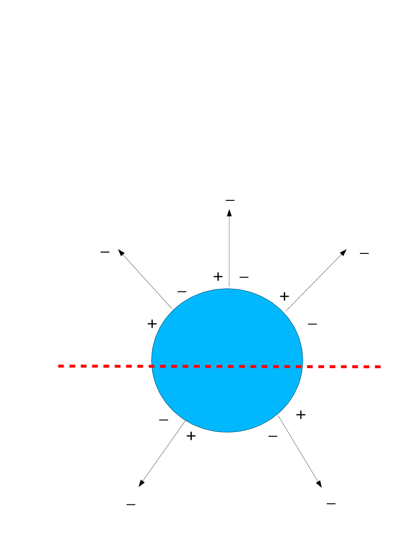
Figure 3: One of the MHV diagrams for the $\langle\,-\,-\,-\,-\,-\,\rangle$ process. The tree-level diagrams on both side of the cuts are of the type $-\cdots-\,+$, and hence vanish.

Finally, we remark that assuming that amplitudes should be constructible from cut diagrams and MHV tree vertices, the amplitudes $\langle\mp\,+\cdots+\rangle$ are then trivially zero at one loop since they cannot be made from two or more MHV vertices.

7 Conclusions

In this paper we have shown that supersymmetric MHV amplitudes at one loop can be obtained by using the tree level MHV diagrams as vertices, complemented by the CSW prescription to take some of the external lines off shell, when these lines form part of an internal loop. The Feynman rules for the combination of MHV vertices into one-loop diagrams yield a sum over terms which precisely corresponds to the sum over terms in the dispersion relation realization of the one-loop amplitude. This appears rather remarkable, and is an appealing feature which one might expect to persist in more general calculations.

In particular, one would naturally seek to extend this work to compute next-to-maximal helicity violating amplitudes in ${\cal N}=4$ super Yang-Mills at one loop using MHV vertices, which are only known up to $n=6$ external legs. Further applications would be to compute more general non-MHV amplitudes for an arbitrary number of external gluons, as well as the computation of higher-loop gauge theory amplitudes, and the study of theories with less supersymmetry.

Let us also mention that our analysis provides a representation (5.16) of the “two easy masses” box function $F$ in (2.9) expressed in terms of only four dilogarithms and with no logarithms:

$$F(s,t,P^{2},Q^{2}) = -\frac{1}{\epsilon^{2}}\Big{[}(-s)^{-\epsilon}\,+\,(-t)^{-\epsilon}\,-\,(-P^{2})^{-\epsilon}\,-\,(-Q^{2})^{-\epsilon}\Big{]}$$

$$+ {\rm Li}_{2}(1-aP^{2})\,+\,{\rm Li}_{2}(1-aQ^{2})\,-\,{\rm Li}_{2}(1-as)\,-\,{\rm Li}_{2}(1-at)\ ,$$

where

$$a\ =\ \frac{P^{2}+Q^{2}-s-t}{P^{2}Q^{2}-st}\ =\ \frac{u}{P^{2}Q^{2}-st}\ .$$ (7.3)

It seems likely that this new, simpler representation will provide clues as to the correct twistor space description of ${\cal N}=4$ super Yang-Mills, and might simplify the form of other loop amplitudes.

Finally, it is intriguing that the one-loop expression (2.3) for the MHV amplitudes is a sum of box integrals - each with coefficient one. In term of the construction with MHV vertices, this comes only after elaborating the initial expression (by multiple applications of the Schouten identity), and appropriately collecting cut box integrals in order to reconstruct, from the dispersion integrals of the different cuts, the full box function. It would be remarkable if one could find a (string?) theory where the box diagrams represented in Figure 2 themselves have a more fundamental and direct meaning as “Feynman diagrams” emerging from a perturbative description.

References

- [1] E. Witten, Perturbative gauge theory as a string theory in twistor space, hep-th/0312171.
- [2] R. Roiban, M. Spradlin and A. Volovich, A googly amplitude from the B-model in twistor space, JHEP 0404 (2004) 012, hep-th/0402016.
- [3] N. Berkovits, An Alternative String Theory in Twistor Space for Super-Yang-Mills, hep-th/0402045.
- [4] R. Roiban and A. Volovich, All googly amplitudes from the B-model in twistor space, hep-th/0402121.
- [5] A. Neitzke and C. Vafa, Strings and the Twistorial Calabi-Yau, hep-th/0402128.
- [6] F. Cachazo, P. Svrcek and E. Witten, MHV vertices and tree amplitudes in gauge theory, hep-th/0403047.
- [7] C. J. Zhu, The googly amplitudes in gauge theory, JHEP 0404 (2004) 032, hep-th/0403115.
- [8] N. Nekrasov, H. Ooguri and C. Vafa, S-duality and Topological Strings, hep-th/0403167.
- [9] N. Berkovits and L. Motl, Cubic Twistorial String Field Theory, J. High Energy Phys. 0404 (2004) 056, hep-th/0403187.
- [10] R. Roiban, M. Spradlin and A. Volovich, On the tree-level S-matrix of Yang-Mills theory, hep-th/0403190.
- [11] M. Aganagic and C. Vafa, Mirror Symmetry and Supermanifolds, hep-th/0403192.
- [12] E. Witten, Parity Invariance For Strings In Twistor Space, hep-th/0403199.
- [13] G. Georgiou and V. V. Khoze, Tree amplitudes in gauge theory as scalar MHV diagrams, JHEP 0405 (2004) 070, hep-th/0404072.
- [14] S. Gukov, L. Motl and A. Neitzke, Equivalence of twistor prescriptions for super Yang-Mills, hep-th/0404085.
- [15] S. Giombi, R. Ricci, D. Robles-Llana and D. Trancanelli, A Note on Twistor Gravity Amplitudes, hep-th/0405086.
- [16] A.D. Popov and C. Saemann, On Supertwistors, the Penrose-Ward Transform and super Yang-Mills Theory, hep-th/0405123.
- [17] S. Prem Kumar and G. Policastro, Strings in Twistor Superspace and Mirror Symmetry, hep-th/0405236.
- [18] W. Siegel, Untwisting the twistor superstring, hep-th/0405255.
- [19] N. Berkovits and E. Witten, Conformal Supergravity in Twistor-String Theory, hep-th/0406051.
- [20] J-B. Wu and C-J Zhu, MHV Vertices and Scattering Amplitudes in Gauge Theory, hep-th/0406085.
- [21] I. Bena, Z. Bern and D. A. Kosower, Twistor-space recursive formulation of gauge theory amplitudes, hep-th/0406133.
- [22] J-B. Wu and C-J Zhu, MHV Vertices and Fermionic Scattering Amplitudes in Gauge Theory with Quarks and Gluinos, hep-th/0406146.
- [23] D. Kosower, Next-to-Maximal Helicity Violating Amplitudes in Gauge Theory, hep-th/0406175.
- [24] G. Georgiou, E. W. N. Glover and V. V. Khoze, Non-MHV Tree Amplitudes in Gauge Theory, hep-th/0407027.
- [25] F. Cachazo, P. Svrcek and E. Witten, Twistor space structure of one loop amplitudes in gauge theory, hep-th/0406177.
- [26] S. J. Parke and T. R. Taylor, An Amplitude For N Gluon Scattering, Phys. Rev. Lett. 56 (1986) 2459.
- [27] F. A. Berends and W. T. Giele, Recursive Calculations For Processes With N Gluons, Nucl. Phys. B 306 (1988) 759.
- [28] Z. Bern, String-Based Perturbative Methods for Gauge Theories, TASI Lectures 1992, hep-ph/9304249.
- [29] Z. Bern, L. J. Dixon, D. C. Dunbar and D. A. Kosower, One Loop N Point Gauge Theory Amplitudes, Unitarity And Collinear Limits, Nucl. Phys. B 425 (1994) 217, hep-ph/9403226.
- [30] Z. Bern, L. J. Dixon, D. C. Dunbar and D. A. Kosower, Fusing gauge theory tree amplitudes into loop amplitudes, Nucl. Phys. B 435 (1995) 59, hep-ph/9409265.
- [31] Z. Bern and A.G. Morgan, Massive Loop Amplitudes from Unitarity, Nucl. Phys. B467 (1996) 479-509, hep-ph/9511336.
- [32] L. J. Dixon, Calculating scattering amplitudes efficiently, TASI Lectures 1995, hep-ph/9601359.
- [33] Z. Bern, L. J. Dixon and D. A. Kosower, Progress in one-loop QCD computations, Ann. Rev. Nucl. Part. Sci. 46 (1996) 109, hep-ph/9602280.
- [34] Z. Bern, L. J. Dixon and D. A. Kosower, Unitarity-based Techniques for One-Loop Calculations in QCD, Nucl. Phys. Proc. Suppl. 51C (1996) 243-249, hep-ph/9606378.
- [35] Z. Bern, A. De Freitas and L. J. Dixon, Two-loop helicity amplitudes for quark gluon scattering in QCD and gluino gluon scattering in supersymmetric Yang-Mills theory, JHEP 0306 (2003) 028, hep-ph/0304168.
- [36] C. Anastasiou, Z. Bern, L. J. Dixon and D. A. Kosower, Planar amplitudes in maximally supersymmetric Yang-Mills theory, Phys. Rev. Lett. 91 (2003) 251602, hep-th/0309040.
- [37] C. Anastasiou, L. J. Dixon, Z. Bern and D. A. Kosower, Cross-order relations in N = 4 supersymmetric gauge theories, in Proceedings of the 3rd International Symposium on Quantum Theory and Symmetries (QTS3), Cincinnati, Ohio, 2003, hep-th/0402053.
- [38] Z. Bern, L. J. Dixon and D. A. Kosower, Two-Loop g gg Splitting Amplitudes in QCD, hep-ph/0404293.
- [39] R. J. Eden, P. V. Landshoff, D. I. Olive and J. C. Polkinghorne, The Analytic S-Matrix, Cambridge University Press, 1966.
- [40] V. P. Nair, A Current Algebra For Some Gauge Theory Amplitudes, Phys. Lett. B 214 (1988) 215.
- [41] R. E. Cutkosky, Singularities And Discontinuities Of Feynman Amplitudes, J. Math. Phys. 1 (1960) 429.
- [42] G. ’t Hooft and M. J. G. Veltman, Regularization And Renormalization Of Gauge Fields, Nucl. Phys. B 44 (1972) 189.
- [43] W. L. van Neerven, Dimensional Regularization Of Mass And Infrared Singularities In Two Loop On-Shell Vertex Functions, Nucl. Phys. B 268 (1986) 453.
- [44] W. Beenakker, H. Kuijf, W. L. van Neerven and J. Smith, QCD Corrections To Heavy Quark Production In P Anti-P Collisions, Phys. Rev. D 40 (1989) 54.
- [45] T. Binoth, J. P. Guillet and G. Heinrich, Reduction formalism for dimensionally regulated one-loop N-point integrals, Nucl. Phys. B 572 (2000) 361, hep-ph/9911342.
- [46] The Wolfram functions site, http://functions.wolfram.com.