July 2004 hep-th/0407211

Abstract

We derive the master function governing the component action of the four-dimensional non-anticommutative (NAC) and fully N=2 supersymmetric gauge field theory with a non-simple gauge group $U(2)=SU(2)\times U(1)$. We use a Lorentz-singlet NAC-deformation parameter and an N=2 supersymmetric star (Moyal) product, which do not break any of the fundamental symmetries of the undeformed N=2 gauge theory. The scalar potential in the NAC-deformed theory is calculated. We also propose the non-abelian BPS-type equations in the case of the NAC-deformed N=2 gauge theory with the $SU(2)$ gauge group, and comment on the $SU(3)$ case too. The NAC-deformed field theories can be thought of as the effective (non-perturbative) N=2 gauge field theories in a certain (scalar only) N=2 supergravity background.

1 Introduction

Noncommutative spaces were extensively studied in the past. The simplest and best known example of noncommutativity is provided by the phase space coordinates in quantum mechanics. In quantum field theory, both at the perturbative and non-perturbative level, the assumption of spacetime noncommutativity is known to lead to new physical phenomena, such as UV/IR mixing, noncommutative solitons, quantum Hall fluid, etc. (see e.g., refs. [1, 2] for a review and an extensive list of references). The spacetime noncommutativity introduces non-locality into field theory in a mild and controllable manner. In particular, a noncommutative field theory still possesses a chiral ring, and there exists a change of variables (the so-called Seiberg-Witten map) that brings the gauge transformations to the standard form [3, 4].

Supersymmetric gauge field theories in Non-AntiCommutative (NAC) superspace [5] is a rather new area of research [6]. Those NAC-deformed field theories naturally arise from superstrings in certain supergravity backgrounds, being natural extensions of the usual (undeformed) supersymmetric gauge field theories. In string theory the noncommutativity of bosonic spacetime coordinates naturally emerges in a (multiple) D-brane worldvolume, when a constant NS–NS two-form is turned on [3]. More recently, in the context of the Dijkgraaf-Vafa correspondence [7] relating N=1 supersymmetric gauge theories and matrix models, it was suggested [8] that the non-anticommutativity of superspace coordinates naturally appears in a D-brane worldvolume when a constant RR two-form is turned on in ten dimensions (see also ref. [9]). A similar phenomenon was discovered in four dimensions when a constant self-dual graviphoton field strength is taken as a superstring background [4].

Fermionic non-anticommutativity means that the odd superspace coordinates obey a Clifford algebra instead of being anticommuting [5]. It is also possible to keep the commutativity of the bosonic spacetime coordinates, which renders the NAC-deformed field theory much more tractable [4]. Consistency implies that merely a chiral part of the fermionic superspace coordinates should become NAC, whereas the anti-chiral fermionic superspace coordinates should be kept anticommuting (in some basis). This is only possible when the anti-chiral fermionic coordinates $(\bar{\theta})$ are not complex conjugates to the chiral ones, $\bar{\theta}\neq(\theta)^{*}$, which is the case in Euclidean and Atiyah-Ward spacetimes with the signature $(4,0)$ and $(2,2)$, respectively. The Euclidean signature is relevant to instantons and superstrings [1, 6], whereas the Atiyah-Ward signature is relevant to the critical N=2 string models [10] and the supersymmetric self-dual gauge field theories [11].

Extended supersymmetry offers more opportunities depending upon how much of supersymmetry one wants to preserve, as well as which NAC deformation (e.g., a singlet or a non-singlet) and which operators (the supercovariant derivatives or the supersymmetry generators) one wants to employ in the Moyal-Weyl star product [5, 12]. The $N=(1,1)$ (or just $N=2$) extended supersymmetry is very special in that respect since it allows one to choose a singlet NAC deformation and a star product that preserve all the fundamental symmetries [13]. Indeed, the most general nilpotent deformation of $N=(1,1)=2\times({{{1}\over{2}}},{{{1}\over{2}}})$ supersymmetry is given by

$$\{\theta_{i}^{\alpha},\theta_{j}^{\beta}\}_{\star}=\delta^{(\alpha\beta)}_{(ij)}C^{(\alpha\beta)}-2iP\varepsilon^{\alpha\beta}\varepsilon_{ij}\quad{\rm(no~{}sum!)}~{},$$

where $\alpha,\beta=1,2$ are chiral spinor indices, $i,j=1,2$ are the indices of the internal R-symmetry group $SU(2)_{R}$, while $C^{\alpha\beta}$ and $P$ are some constants. Taking only a singlet deformation to be non-vanishing, $P\neq 0$, and using the chiral supercovariant N=2 superspace derivatives $D_{i\alpha}$ in the Moyal-Weyl star product,

$$A\star B=A\exp\left(iP\varepsilon^{\alpha\beta}\varepsilon^{ij}\mathop{\hbox{}D}\limits^{\leftarrow}{}_{i\alpha}\vec{D}{}_{j\beta}\right)B~{}~{},$$

allows one to keep manifest N=2 supersymmetry, Lorentz invariance and R-invariance, as well as (undeformed) gauge invariance (after some non-linear field redefinition) [13]. The star product (1.2) matching those conditions is unique, and it requires $N=2$.

We choose flat Euclidean spacetime for definiteness, but continue to use the notation common to N=2 superspace with Minkowski spacetime signature, as it is becoming increasingly customary in the current literature (see also ref. [14] for more details about our notation). Our NAC N=2 superspace with the coordinates $(x^{m},\theta^{i}_{\alpha},\bar{\theta}_{i}^{\buildrel{}_{{}_{\hskip 0.72229pt}\bullet}\over{\alpha}})$ is defined by eq. (1.1), with $C^{\alpha\beta}=0$ and $P\neq 0$, as the only non-trivial (anti)commutator amongst the N=2 superspace coordinates. This choice preserves all most fundamental symmetries and features of N=2 supersymmetry including the so-called G-analyticity [13].

A NAC-deformed (non-abelian) supersymmetric gauge field theory can also be rewritten to the usual form, with the standard gauge transformations of its field components, i.e. as some kind of effective action, after certain (non-linear) field redefinition known as the Seiberg-Witten map (cf. ref. [3]). In the case of the $P$-deformed N=2 super-Yang-Mills theory such (non-abelian) map was calculated by Ferrara and Sokatchev in ref. [13] with the following result for the effective anti-chiral N=2 superfield strength:

$$\overline{W}_{\rm NAC}={{\overline{W}}\over{1+P\overline{W}}}~{}~{}.$$

Here $\overline{W}$ is the standard (Lie algebra-valued) covariant N=2 superfield strength subject to the standard N=2 superspace Bianchi identities

$${\cal D}_{i\alpha}\overline{W}=0\qquad{\rm and}\qquad{\cal D}_{ij}W=\overline{{\cal D}}_{ij}\overline{W}~{}~{},$$

in terms of the N=2 superspace gauge- and super-covariant derivatives ${\cal D}^{i\alpha}$ and $\overline{{\cal D}}_{i\buildrel{}_{{}_{\hskip 0.72229pt}\bullet}\over{\alpha}}$, obeying an algebra

$$\{{\cal D}^{i}_{\alpha},{\cal D}^{j}_{\beta}\}=-2\varepsilon^{ij}\varepsilon_{\alpha\beta}\overline{W}~{}.$$

We use the notation ${\cal D}{\raise-3.0pt\hbox{${\hskip 0.75pt}\!_{ij}$}}={\cal D}^{\alpha}{\raise-3.0pt\hbox{${\hskip 0.75pt}\!_{(i}$}}{\cal D}{\raise-3.0pt\hbox{${\hskip 0.75pt}\!_{j)\alpha}$}}$ and $\overline{{\cal D}}{\raise-3.0pt\hbox{${\hskip 0.75pt}\!_{ij}$}}=\overline{{\cal D}}_{\buildrel{}_{{}_{\hskip 0.72229pt}\bullet}\over{\alpha}(i}\overline{{\cal D}}^{\buildrel{}_{{}_{\hskip 0.72229pt}\bullet}\over{\alpha}}{\raise-3.0pt\hbox{${\hskip 0.75pt}\!_{j)}$}}$, and define the covariant field components of the N=2 superfield $\overline{W}$ by covariant differentiation,

$$\overline{W}|=\bar{\phi}~{},\quad\overline{{\cal D}}_{i\buildrel{}_{{}_{\hskip 0.72229pt}\bullet}\over{\alpha}}\overline{W}|=\bar{\lambda}_{i\buildrel{}_{{}_{\hskip 0.72229pt}\bullet}\over{\alpha}}~{},\quad\overline{{\cal D}}_{ij}\overline{W}|=D_{ij}~{},\quad\overline{{\cal D}}_{\buildrel{}_{{}_{\hskip 0.72229pt}\bullet}\over{\alpha}\buildrel{}_{{}_{\hskip 0.72229pt}\bullet}\over{\beta}}\overline{W}|=F_{\buildrel{}_{{}_{\hskip 0.72229pt}\bullet}\over{\alpha}\buildrel{}_{{}_{\hskip 0.72229pt}\bullet}\over{\beta}}~{},$$

where $|$ denotes the leading ($\theta$- and $\bar{\theta}$-independent) component of an N=2 superfield.

The effective N=2 superspace action reads

$$S_{\rm NAC}=\hbox{\large{${{\textstyle{{1}\over\vphantom{2}\smash{\raise 0.72331pt\hbox{$\scriptstyle{{2}}$}}}}}$}}\int d^{4}x{\raise-3.0pt\hbox{${\hskip 0.75pt}\!_{R}$}}d^{4}\bar{\theta}\,{\rm Tr}\,\overline{W}^{2}_{\rm NAC}\equiv\hbox{\large{${{\textstyle{{1}\over\vphantom{2}\smash{\raise 0.72331pt\hbox{$\scriptstyle{{2}}$}}}}}$}}\int d^{4}x{\raise-3.0pt\hbox{${\hskip 0.75pt}\!_{R}$}}d^{4}\bar{\theta}\,{\rm Tr}f(\overline{W})~{},$$

whose structure function $f(\overline{W})$ follows from eq. (1.3),

$$f(\overline{W})=\left({{\overline{W}}\over{1+P\overline{W}}}\right)^{2}~{}~{}.$$

It is non-trivial to calculate the action (1.7) in components because of the need to perform the (non-abelian) group-theoretical trace (the Lagrangian is no longer quadratic in $\overline{W}\,$!). The case of the NAC, N=2 supersymmetric gauge field theory with an (abelian) $U(1)$ gauge group is, of course, fully straightforward because its master function, governing the action of its field components after taking the group-theoretical trace, is still given by the same function (1.8) — see e.g., ref. [13]. The full equations of motion in the NAC-deformed abelian N=2 theory, as well as their BPS-like counterparts, were calculated in our earlier paper [15]. The master function in the simplest non-abelian, NAC and N=2 supersymmetric gauge field theory with the gauge group $SU(2)$ was found in ref. [16]. In this paper we calculate the master function of the NAC four-dimensional N=2 supersymmetric gauge field theory having a non-simple gauge group $U(2)=SU(2)\times U(1)$. Our new solution interpolates between the master functions found in refs. [13, 15] and [16].

Our paper is organized as follows. In sect. 2 we perform the $U(2)$ group-theoretical trace in eq. (1.7) in order to find the master function of the colorless variables $\overline{W}^{a}\overline{W}^{a}$ and $\overline{W}{}^{0}$ associated with the $SU(2)$ and $U(1)$ factors, respectively, which governs the full component action. In sect. 3 we show how our results reduce to the known master functions for the $SU(2)$ and $U(1)$ gauge groups, separately [15, 16]. We also give some new results about the BPS equations in the (non-abelian) $SU(2)$ case. In sect. 4 we calculate the scalar potential in the deformed $U(2)$ theory. Sect. 5 is our conclusion that includes a short discussion of the $SU(3)$ case too.

2 Calculation of the $U(2)$ trace

In the $U(2)$ case we find convenient to use the hermitian $3\times 3$ matrices  both for the $U(1)$ and the $SU(2)$ generators, namely,

$$T^{0}=\left(\begin{array}[]{ccc}1&0&0\\ 0&1&0\\ 0&0&1\end{array}\right)$$

and

$$T^{1}=\left(\begin{array}[]{ccc}0&0&0\\ 0&0&-i\\ 0&i&0\end{array}\right)~{}~{},\quad T^{2}=\left(\begin{array}[]{ccc}0&0&i\\ 0&0&0\\ -i&0&0\end{array}\right)~{}~{},\quad T^{3}=\left(\begin{array}[]{ccc}0&-i&0\\ i&0&0\\ 0&0&0\end{array}\right)~{}~{},$$

respectively, which obey the commutation relations $\lfloor{\hskip 0.35pt}\!\!\!\lceil T^{a},T^{b}\rfloor{\hskip 0.35pt}\!\!\!\rceil=i\varepsilon^{abc}T^{c}$, where $\varepsilon^{abc}$ is the totally antisymmetric Levi-Civita symbol with $\varepsilon^{123}=1$ and $a,b,\ldots=1,2,3$.

The master function in the $U(2)$ case under investigation is given by

  $${h(\overline{W}{}^{0},\overline{W}{}^{a})} {{}\equiv{\rm Tr}\left[f(\overline{W}{}^{a}T^{a}+\overline{W}{}^{0}T^{0})\right]={\rm Tr}\left[{{\overline{W}{}^{a}T^{a}+\overline{W}{}^{0}T^{0}}\over{1+P(\overline{W}{}^{a}T^{a}+\overline{W}{}^{0}T^{0})}}\right]^{2}} {{}=\sum^{+\infty}_{n=0}(n+1)(-)^{n}P^{n}{\rm Tr}\,G^{n+2}~{},}$$  

where we have introduced the notation

$$G=\overline{W}{}^{a}T^{a}+\overline{W}{}^{0}T^{0}~{},$$

and ${\rm Tr}$ stands for the group-theoretical trace. In particular, we have

$${\rm Tr}\,G^{n}={\rm Tr}\left(\overline{W}{}^{a}T^{a}+\overline{W}{}^{0}T^{0}\right)^{n}={\rm Tr}\sum^{n}_{r=0}\left(\begin{array}[]{c}n\\ r\end{array}\right)(\overline{W}{}^{a}T^{a})^{n-r}(\overline{W}{}^{0}T^{0})^{r}~{}~{},$$

where

$$\left(\begin{array}[]{c}n\\ r\end{array}\right)={{n!}\over{r!(n-r)!}}~{}.$$

The basic $SU(2)$ traces were already computed in ref. [16],

$${\rm Tr}(\overline{W}{}^{a}T^{a})^{2m}=2(\overline{W}{}^{a}\overline{W}{}^{a})^{m}~{},~{}~{}m>0,\quad{\rm Tr}(\overline{W}{}^{a}T^{a})^{0}=3~{},\quad{\rm Tr}(\overline{W}{}^{a}T^{a})^{2m-1}=0~{},$$

so that it is useful to compute the sums over the even and odd powers of $P$ in eq. (2.2) separately. As regards the sum over all even powers of $P$ on the right-hand-side of eq. (2.2), we find

$$\sum^{\infty}_{m=1}\sum^{m}_{r=0}(2m-1)P^{2m-2}\left(\begin{array}[]{c}2m\\ 2r\end{array}\right)(\overline{W}{}^{0})^{2r}{\rm Tr}(\overline{W}{}^{a}T^{a})^{2(m-r)}=\sum^{\infty}_{m=1}{{2m-1}\over{P^{2}}}(P^{2}\overline{W}{}^{0}\overline{W}{}^{0})^{m}$$

$$+\sum^{\infty}_{m=1}{{2m-1}\over{P^{2}}}\left[P^{2}\overline{W}{}^{0}\overline{W}{}^{0}\left(1-\sqrt{{{\overline{W}{}^{0}\overline{W}{}^{0}}\over{\overline{W}{}^{a}\overline{W}{}^{a}}}}\right)^{2}\right]^{m}$$

$$+\sum^{\infty}_{m=1}{{2m-1}\over{P^{2}}}\left[P^{2}\overline{W}{}^{0}\overline{W}{}^{0}\left(1+\sqrt{{{\overline{W}{}^{0}\overline{W}{}^{0}}\over{\overline{W}{}^{a}\overline{W}{}^{a}}}}\right)^{2}\right]^{m}~{}~{},$$

where we have used the identity

$$\sum^{m-1}_{r=0}\left(\begin{array}[]{c}2m\\ 2r\end{array}\right)x^{r}=\hbox{\large{${{\textstyle{{1}\over\vphantom{2}\smash{\raise 0.72331pt\hbox{$\scriptstyle{{2}}$}}}}}$}}\left[(1-\sqrt{x})^{2m}+(1+\sqrt{x})^{2m}-2x^{m}\right]~{}.$$

Next, when using the identities

$$\sum^{\infty}_{m=1}x^{m}={{x}\over{1-x}}\quad{\rm and}\quad\sum^{\infty}_{m=1}mx^{m}={{x}\over{(1-x)^{2}}}~{}~{}~{}~{},$$

we can rewrite eq. (2.7) to the form

  $${{}~{}{{\overline{W}{}^{0}\overline{W}{}^{0}(1+P^{2}\overline{W}{}^{0}\overline{W}{}^{0})}\over{(1-P^{2}\overline{W}{}^{0}\overline{W}{}^{0})^{2}}}~{}~{}+} {+~{}~{}} {{}~{}{{1+P^{2}\overline{W}{}^{a}\overline{W}{}^{a}\left(1-\sqrt{{{\overline{W}{}^{0}\overline{W}{}^{0}}\over{\overline{W}{}^{a}\overline{W}{}^{a}}}}\right)^{2}}\over{\left[1-P^{2}\overline{W}{}^{a}\overline{W}{}^{a}\left(1-\sqrt{{{\overline{W}{}^{0}\overline{W}{}^{0}}\over{\overline{W}{}^{a}\overline{W}{}^{a}}}}\right)^{2}\right]^{2}}}\overline{W}{}^{a}\overline{W}{}^{a}\left(1-\sqrt{{{\overline{W}{}^{0}\overline{W}{}^{0}}\over{\overline{W}{}^{a}\overline{W}{}^{a}}}}\right)^{2}~{}~{}+} {+~{}~{}} {{}~{}{{1+P^{2}\overline{W}{}^{a}\overline{W}{}^{a}\left(1+\sqrt{{{\overline{W}{}^{0}\overline{W}{}^{0}}\over{\overline{W}{}^{a}\overline{W}{}^{a}}}}\right)^{2}}\over{\left[1+P^{2}\overline{W}{}^{a}\overline{W}{}^{a}\left(1+\sqrt{{{\overline{W}{}^{0}\overline{W}{}^{0}}\over{\overline{W}{}^{a}\overline{W}{}^{a}}}}\right)^{2}\right]^{2}}}\overline{W}{}^{a}\overline{W}{}^{a}\left(1+\sqrt{{{\overline{W}{}^{0}\overline{W}{}^{0}}\over{\overline{W}{}^{a}\overline{W}{}^{a}}}}\right)^{2}~{}~{}~{}~{}.}$$  

Similarly, the sum over odd powers of $P$ on the right-hand-side of eq. (2.2) is given by

$$\sum^{\infty}_{m=1}\sum^{m}_{r=0}2mP^{2m-1}\left(\begin{array}[]{c}2m+1\\ 2r+1\end{array}\right)(\overline{W}{}^{0})^{2r+1}{\rm Tr}(\overline{W}{}^{a}T^{a})^{2(m-r)}={{2P(\overline{W}{}^{0})^{3}}\over{(1-P^{2}\overline{W}{}^{0}\overline{W}{}^{0})^{2}}}~{}~{}+$$

$$+~{}\left(1+{{1}\over{\sqrt{{{\overline{W}{}^{0}\overline{W}{}^{0}}\over{\overline{W}{}^{a}\overline{W}{}^{a}}}}}}\right){{2P\overline{W}{}^{0}(\overline{W}{}^{a}\overline{W}{}^{a})\left(1+\sqrt{{{\overline{W}{}^{0}\overline{W}{}^{0}}\over{\overline{W}{}^{a}\overline{W}{}^{a}}}}\right)^{2}}\over{\left[1-P^{2}(\overline{W}{}^{a}\overline{W}{}^{a})\left(1+\sqrt{{{\overline{W}{}^{0}\overline{W}{}^{0}}\over{\overline{W}{}^{a}\overline{W}{}^{a}}}}\right)^{2}\right]^{2}}}~{}~{}+$$

$$+~{}\left(1-{{1}\over{\sqrt{{{\overline{W}{}^{0}\overline{W}{}^{0}}\over{\overline{W}{}^{a}\overline{W}{}^{a}}}}}}\right){{2P\overline{W}{}^{0}(\overline{W}{}^{a}\overline{W}{}^{a})\left(1-\sqrt{{{\overline{W}{}^{0}\overline{W}{}^{0}}\over{\overline{W}{}^{a}\overline{W}{}^{a}}}}\right)^{2}}\over{\left[1-P^{2}(\overline{W}{}^{a}\overline{W}{}^{a})\left(1-\sqrt{{{\overline{W}{}^{0}\overline{W}{}^{0}}\over{\overline{W}{}^{a}\overline{W}{}^{a}}}}\right)^{2}\right]^{2}}}~{}~{}~{}~{},$$

where we have used yet another identity

  $${\sum^{m-1}_{r=0}\left(\begin{array}[]{c}2m+1\\ 2r+1\end{array}\right)x^{r}=~{}} {{}{{1}\over{2}}\left[(1+\sqrt{x})^{2m}+(1-\sqrt{x})^{2m}\right]~{}+} {{}+{{1}\over{2\sqrt{x}}}\left[(1+\sqrt{x})^{2m}-(1-\sqrt{x})^{2m}\right]-x^{m}~{},}$$  

together with eqs. (2.6) and (2.9). The final result for the $U(2)$ master function is given by a sum of eqs. (2.10) and (2.11), which reads

  $${h(\overline{W}{}^{0},\overline{W}{}^{a})=} {{}\left({{\overline{W}{}^{0}}\over{1+P\overline{W}{}^{0}}}\right)^{2}~{}+} {{}+\left[{{\overline{W}{}^{0}+\sqrt{\overline{W}{}^{a}\overline{W}{}^{a}}}\over{1+P\left(\overline{W}{}^{0}+\sqrt{\overline{W}{}^{a}\overline{W}{}^{a}}\right)}}\right]^{2}+\left[{{\overline{W}{}^{0}-\sqrt{\overline{W}{}^{a}\overline{W}{}^{a}}}\over{1+P\left(\overline{W}{}^{0}-\sqrt{\overline{W}{}^{a}\overline{W}{}^{a}}\right)}}\right]^{2}~{}~{}.}$$  

This equation is one of the main new results of our paper, because it is needed for a straightforward calculation of the component action out of eqs. (1.6) and (1.7).

3 Some limits, and non-abelian BPS equations

In this section we are going to demonstrate how some earlier established results [13, 15, 16] follow from our general equation (2.13), as well as find new (non-abelian) BPS equations in the NAC, N=2 theory with the $SU(2)$ gauge group.

(i) Firstly, as regards the commutative limit $P\to 0$, we easily find

  $${\lim_{P\to 0}h(\overline{W}{}^{0},\overline{W}{}^{a})} {{}~{}=\left(\overline{W}{}^{0}\right)^{2}+\left(\overline{W}{}^{0}+\sqrt{\overline{W}{}^{a}\overline{W}{}^{a}}\right)^{2}+\left(\overline{W}{}^{0}-\sqrt{\overline{W}{}^{a}\overline{W}{}^{a}}\right)^{2}} {{}~{}=3(\overline{W}{}^{0})^{2}+2\overline{W}{}^{a}\overline{W}{}^{a}={\rm Tr}(\overline{W}{}^{a}T^{a}+\overline{W}{}^{0}T^{0})^{2}~{}~{}.}$$  

This reproduces the usual (commutative) N=2 supersymmetric $U(2)$ gauge theory, as it should.

(ii) Second, let us consider another limit, $\overline{W}{}^{0}\to 0$. In this case eq. (2.13) yields

  $${\lim_{\overline{W}{}^{0}\to 0}h(\overline{W}{}^{0},\overline{W}{}^{a})} {{}~{}=\left({{\sqrt{\overline{W}{}^{a}\overline{W}{}^{a}}}\over{1+P\sqrt{\overline{W}{}^{a}\overline{W}{}^{a}}}}\right)^{2}+\left({{-\sqrt{\overline{W}{}^{a}\overline{W}{}^{a}}}\over{1-P\sqrt{\overline{W}{}^{a}\overline{W}{}^{a}}}}\right)^{2}} {{}~{}={{2\overline{W}{}^{a}\overline{W}{}^{a}+2P^{2}(\overline{W}{}^{a}\overline{W}{}^{a})^{2}}\over{(1-P^{2}\overline{W}{}^{a}\overline{W}{}^{a})^{2}}}~{}~{}.}$$  

This result precisely reproduces the master function in the NAC, N=2 supersymmetric Yang-Mills theory with the gauge group $SU(2)$, which was calculated in ref. [16].

(iii) Third, in the NAC abelian limit $\overline{W}{}^{a}\to 0$, we find from eq. (2.13) that

  $${\lim_{\overline{W}{}^{a}\to 0}h(\overline{W}{}^{0},\overline{W}{}^{a})} {{}~{}=\left({{\overline{W}{}^{0}}\over{1+P\overline{W}{}^{0}}}\right)^{2}+2\left({{\overline{W}{}^{0}}\over{1+P\overline{W}{}^{0}}}\right)^{2}} {{}~{}=3\left({{\overline{W}{}^{0}}\over{1+P\overline{W}{}^{0}}}\right)^{2}={\rm Tr}\left({{\overline{W}{}^{0}{\bf 1}}\over{{\bf 1}+P\overline{W}{}^{0}{\bf 1}}}\right)^{2}~{}~{},}$$  

where ${\bf 1}=T^{0}$ stands for a unit $3\times 3$ matrix. Equation (3.3) precisely reproduces the NAC, N=2 supersymmetric gauge theory with the abelian gauge group $U(1)$ [13, 15].

The BPS equations in the non-anticommutative N=2 supersymmetric gauge theory with the abelian gauge group $U(1)$ were derived in ref. [15]. To this end, we would like to derive the non-abelian BPS equations, by considering the non-anticommutative N=2 gauge theory with a simple gauge group $SU(2)$ for simplicity. The component Lagrangian of this theory was calculated in ref. [15] by decomposing the relevant N=2 anti-chiral superfield $\overline{W}{}^{2}\equiv\overline{W}{}^{a}\overline{W}{}^{a}$ as follows (in the anti-chiral N=2 basis):

$$\overline{W}{}^{2}=U+V_{\buildrel{}_{{}_{\hskip 0.72229pt}\bullet}\over{\alpha}i}\bar{\theta}^{\buildrel{}_{{}_{\hskip 0.72229pt}\bullet}\over{\alpha}i}+X_{ij}\bar{\theta}^{ij}+Y_{\buildrel{}_{{}_{\hskip 0.72229pt}\bullet}\over{\alpha}\buildrel{}_{{}_{\hskip 0.72229pt}\bullet}\over{\beta}}\bar{\theta}^{\buildrel{}_{{}_{\hskip 0.72229pt}\bullet}\over{\alpha}\buildrel{}_{{}_{\hskip 0.72229pt}\bullet}\over{\beta}}+Z_{\buildrel{}_{{}_{\hskip 0.72229pt}\bullet}\over{\alpha}i}(\bar{\theta}^{3})^{\buildrel{}_{{}_{\hskip 0.72229pt}\bullet}\over{\alpha}i}+L\bar{\theta}^{4}~{},$$

where we have introduced its (composite) field components $(U,V_{\buildrel{}_{{}_{\hskip 0.72229pt}\bullet}\over{\alpha}i},X_{ij},Y_{\buildrel{}_{{}_{\hskip 0.72229pt}\bullet}\over{\alpha}\buildrel{}_{{}_{\hskip 0.72229pt}\bullet}\over{\beta}},Z_{\buildrel{}_{{}_{\hskip 0.72229pt}\bullet}\over{\alpha}i},L)$. The composites can be expressed in terms of the gauge-covariant field components (1.6) as follows [16]:

$$U=\bar{\phi}^{a}\bar{\phi}^{a},~{}~{}V_{\buildrel{}_{{}_{\hskip 0.72229pt}\bullet}\over{\alpha}i}=2\bar{\lambda}^{a}_{\buildrel{}_{{}_{\hskip 0.72229pt}\bullet}\over{\alpha}i}\bar{\phi}^{a},~{}~{}X_{ij}=2\left(\bar{\phi}^{a}D^{a}_{ij}-\bar{\lambda}^{\buildrel{}_{{}_{\hskip 0.72229pt}\bullet}\over{\alpha}a}_{i}\bar{\lambda}^{a}_{j\buildrel{}_{{}_{\hskip 0.72229pt}\bullet}\over{\alpha}}\right)~{},~{}~{}Y_{\buildrel{}_{{}_{\hskip 0.72229pt}\bullet}\over{\alpha}\buildrel{}_{{}_{\hskip 0.72229pt}\bullet}\over{\beta}}=2\left(\bar{\phi}^{a}F^{a}_{\buildrel{}_{{}_{\hskip 0.72229pt}\bullet}\over{\alpha}\buildrel{}_{{}_{\hskip 0.72229pt}\bullet}\over{\beta}}-\bar{\lambda}^{ia}_{\buildrel{}_{{}_{\hskip 0.72229pt}\bullet}\over{\alpha}}\bar{\lambda}^{a}_{i\buildrel{}_{{}_{\hskip 0.72229pt}\bullet}\over{\beta}}\right)~{},$$

$$Z_{i\buildrel{}_{{}_{\hskip 0.72229pt}\bullet}\over{\alpha}}=4i\bar{\phi}^{a}(\tilde{\sigma}^{\mu})_{\buildrel{}_{{}_{\hskip 0.72229pt}\bullet}\over{\alpha}}{}^{\alpha}{\cal D}_{\mu}\lambda^{a}_{i\alpha}+\bar{\lambda}^{ja}_{\buildrel{}_{{}_{\hskip 0.72229pt}\bullet}\over{\alpha}}D_{ij}-\bar{\lambda}^{\buildrel{}_{{}_{\hskip 0.72229pt}\bullet}\over{\beta}a}_{i}F^{a}_{\buildrel{}_{{}_{\hskip 0.72229pt}\bullet}\over{\alpha}\buildrel{}_{{}_{\hskip 0.72229pt}\bullet}\over{\beta}}~{}~{},$$

and

  $${L=~{}} {{}~{}-2\bar{\phi}^{a}{\cal D}_{\mu}{\cal D}^{\mu}\phi^{a}-i\bar{\lambda}^{a}_{i\buildrel{}_{{}_{\hskip 0.72229pt}\bullet}\over{\alpha}}(\tilde{\sigma}^{\mu})^{\buildrel{}_{{}_{\hskip 0.72229pt}\bullet}\over{\alpha}\alpha}{\cal D}_{\mu}\lambda^{ia}_{\alpha}+\varepsilon^{abc}\lambda^{ia\alpha}\bar{\phi}^{b}\lambda^{c}_{i\alpha}+\varepsilon^{abc}\bar{\lambda}^{a}_{i\buildrel{}_{{}_{\hskip 0.72229pt}\bullet}\over{\alpha}}\phi^{b}\bar{\lambda}^{\buildrel{}_{{}_{\hskip 0.72229pt}\bullet}\over{\alpha}ic}} {{}~{}+{{1}\over{48}}D^{a}_{ij}D^{aij}-{{1}\over{12}}F^{\mu\nu a-}F^{a-}_{\mu\nu}-\hbox{\large{${{\textstyle{{1}\over\vphantom{2}\smash{\raise 0.72331pt\hbox{$\scriptstyle{{2}}$}}}}}$}}\phi^{a}\bar{\phi}^{b}\phi^{c}\bar{\phi}^{d}\varepsilon^{abf}\varepsilon^{cdf}~{},}$$  

where ${\cal D}_{\mu}$ are the usual gauge-covariant derivatives (in the adjoint), $F^{-}_{\mu\nu}$ is the anti-self-dual part of $F_{\mu\nu}$, with $\mu,\nu=1,2,3,4$. The last composite field $L$ is nothing but the usual (undeformed) N=2 super-Yang-Mills Lagrangian, $L={\cal L}_{\rm SYM}$.

The full component action was calculated out of eqs. (1.7) and (3.2) in ref. [15],

  $${{\cal L}_{\rm deformed~{}SYM}=~{}} {{}F(\bar{\phi}^{2}){\cal L}_{\rm SYM}+2F^{\prime}(\bar{\phi}^{2})\left[-4i\bar{\phi}^{a}\bar{\phi}^{b}(\bar{\lambda}^{a}_{i}\tilde{\sigma}^{\mu}{\cal D}_{\mu}\lambda^{ib})+\bar{\phi}^{a}(\bar{\lambda}^{2})^{ab}_{ij}D^{ijb}\right.} {{}+8\bar{\phi}^{a}D^{a}_{ij}(\bar{\lambda}^{2})^{ij}+4\bar{\phi}^{a}\bar{\phi}^{b}D^{a}_{ij}D^{bij}-\bar{\phi}^{a}(\bar{\lambda}^{2})^{ab}_{\buildrel{}_{{}_{\hskip 0.72229pt}\bullet}\over{\alpha}\buildrel{}_{{}_{\hskip 0.72229pt}\bullet}\over{\beta}}(\tilde{\sigma}^{\mu\nu})^{\buildrel{}_{{}_{\hskip 0.72229pt}\bullet}\over{\alpha}\buildrel{}_{{}_{\hskip 0.72229pt}\bullet}\over{\beta}}F^{b-}_{\mu\nu}} {{}\left.-8\bar{\phi}^{a}F^{a-}_{\mu\nu}(\tilde{\sigma}^{\mu\nu})_{\buildrel{}_{{}_{\hskip 0.72229pt}\bullet}\over{\alpha}\buildrel{}_{{}_{\hskip 0.72229pt}\bullet}\over{\beta}}(\bar{\lambda}^{2})^{\buildrel{}_{{}_{\hskip 0.72229pt}\bullet}\over{\alpha}\buildrel{}_{{}_{\hskip 0.72229pt}\bullet}\over{\beta}}-128\bar{\phi}^{a}\bar{\phi}^{b}F^{a-}_{\mu\nu}F^{\mu\nu b-}+96\bar{\lambda}^{4}\right]} {{}+8F^{\prime\prime}(\bar{\phi}^{2})\left[-\bar{\phi}^{a}\bar{\phi}^{b}\bar{\phi}^{c}(\bar{\lambda}^{2})^{ab}_{\buildrel{}_{{}_{\hskip 0.72229pt}\bullet}\over{\alpha}\buildrel{}_{{}_{\hskip 0.72229pt}\bullet}\over{\beta}}(\tilde{\sigma}^{\mu\nu})^{\buildrel{}_{{}_{\hskip 0.72229pt}\bullet}\over{\alpha}\buildrel{}_{{}_{\hskip 0.72229pt}\bullet}\over{\beta}}F^{c-}_{\mu\nu}+\bar{\phi}^{a}\bar{\phi}^{b}\bar{\phi}^{c}(\bar{\lambda}^{2})^{ab}_{ij}D^{ijc}\right.} {{}\left.+24\bar{\phi}^{a}\bar{\phi}^{b}(\bar{\lambda}^{4})^{ab}\right]+16F^{\prime\prime\prime}(\bar{\phi}^{2})\bar{\phi}^{a}\bar{\phi}^{b}\bar{\phi}^{c}\bar{\phi}^{d}(\bar{\lambda}^{4})^{abcd}~{},}$$  

where we have introduced the book-keeping notation 

$$F(\bar{\phi}^{2})={{1-3\tilde{P}^{2}\bar{\phi}^{2}}\over{(1+\tilde{P}^{2}\bar{\phi}^{2})^{3}}}=1-6\tilde{P}^{2}\bar{\phi}^{2}+{\cal O}(\tilde{P}^{4}\bar{\phi}^{4})~{},$$

as well as

  $${(\bar{\lambda}^{2})_{ij}} {{}=\bar{\lambda}^{a}_{i\buildrel{}_{{}_{\hskip 0.72229pt}\bullet}\over{\alpha}}\bar{\lambda}_{j}^{\buildrel{}_{{}_{\hskip 0.72229pt}\bullet}\over{\alpha}a}\quad{\rm and}\quad(\bar{\lambda}^{2})_{\buildrel{}_{{}_{\hskip 0.72229pt}\bullet}\over{\alpha}\buildrel{}_{{}_{\hskip 0.72229pt}\bullet}\over{\beta}}=\bar{\lambda}^{a}_{i\buildrel{}_{{}_{\hskip 0.72229pt}\bullet}\over{\alpha}}\bar{\lambda}^{ia}_{\buildrel{}_{{}_{\hskip 0.72229pt}\bullet}\over{\beta}}~{},} {(\bar{\lambda}^{2})_{ij}^{ab}} {{}=\bar{\lambda}^{a}_{i\buildrel{}_{{}_{\hskip 0.72229pt}\bullet}\over{\alpha}}\bar{\lambda}_{j}^{\buildrel{}_{{}_{\hskip 0.72229pt}\bullet}\over{\alpha}b}\quad{\rm and}\quad(\bar{\lambda}^{2})^{ab}_{\buildrel{}_{{}_{\hskip 0.72229pt}\bullet}\over{\alpha}\buildrel{}_{{}_{\hskip 0.72229pt}\bullet}\over{\beta}}=\bar{\lambda}^{a}_{i\buildrel{}_{{}_{\hskip 0.72229pt}\bullet}\over{\alpha}}\bar{\lambda}^{ib}_{\buildrel{}_{{}_{\hskip 0.72229pt}\bullet}\over{\beta}}~{}~{},} {(\bar{\lambda}^{2})^{ab}} {{}=\bar{\lambda}^{a}_{i\buildrel{}_{{}_{\hskip 0.72229pt}\bullet}\over{\alpha}}\bar{\lambda}^{i\buildrel{}_{{}_{\hskip 0.72229pt}\bullet}\over{\alpha}b}\quad{\rm and}\quad(\bar{\lambda}^{4})^{abcd}=\bar{\lambda}^{1a}_{\buildrel{}_{{}_{\hskip 0.72229pt}\bullet}\over{1}}\bar{\lambda}^{1b}_{\buildrel{}_{{}_{\hskip 0.72229pt}\bullet}\over{2}}\bar{\lambda}^{2c}_{\buildrel{}_{{}_{\hskip 0.72229pt}\bullet}\over{1}}\bar{\lambda}^{2d}_{\buildrel{}_{{}_{\hskip 0.72229pt}\bullet}\over{2}}~{},}$$  

while the primes in eq. (3.6) denote differentiations with respect to the argument $\overline{\phi}^{2}$. The Euler-Lagrange equations of motion of the theory (3.6) can be found in ref. [16].

To illustrate our procedure of deducing BPS equations from a given action, let us first consider only the gauge field-dependent terms in eq. (3.6),

$$L_{\rm gauge}=-g^{ab}F^{a-}_{\mu\nu}F^{\mu\nu b-}+B^{a}_{\mu\nu}F^{\mu\nu a-}~{},$$

where we have introduced the field-dependent ‘metric’ $g^{ab}=g^{ba}$,

$$g^{ab}(\bar{\phi})=\hbox{\large{${{\textstyle{{1}\over\vphantom{2}\smash{\raise 0.72331pt\hbox{$\scriptstyle{{12}}$}}}}}$}}F(\bar{\phi}^{2})\delta^{ab}+2^{8}F^{\prime}(\bar{\phi}^{2})\bar{\phi}^{a}\bar{\phi}^{b}~{}~{},$$

and the antisymmetric (field-dependent) ‘tensor’ $B^{a}_{\mu\nu}=-B^{a}_{\nu\mu}$,

$$B^{a}_{\mu\nu}(\bar{\phi},\bar{\lambda})=-2(\tilde{\sigma}_{\mu\nu})^{\buildrel{}_{{}_{\hskip 0.72229pt}\bullet}\over{\alpha}\buildrel{}_{{}_{\hskip 0.72229pt}\bullet}\over{\beta}}\left[16F(\bar{\phi}^{2})\bar{\phi}^{a}\bar{\lambda}_{\buildrel{}_{{}_{\hskip 0.72229pt}\bullet}\over{\alpha}\buildrel{}_{{}_{\hskip 0.72229pt}\bullet}\over{\beta}}+F^{\prime}(\bar{\phi}^{2})\bar{\phi}^{b}\bar{\lambda}^{ba}_{\buildrel{}_{{}_{\hskip 0.72229pt}\bullet}\over{\alpha}\buildrel{}_{{}_{\hskip 0.72229pt}\bullet}\over{\beta}}+4F^{\prime\prime}(\bar{\phi}^{2})\bar{\phi}^{a}\bar{\phi}^{b}\bar{\phi}^{c}\bar{\lambda}^{bc}_{\buildrel{}_{{}_{\hskip 0.72229pt}\bullet}\over{\alpha}\buildrel{}_{{}_{\hskip 0.72229pt}\bullet}\over{\beta}}\right]~{}.$$

The most naive BPS procedure amounts to forming perfect squares out of the various terms in the Lagrangian, and demanding each squared term to vanish, thus ‘minimizing’ the Euclidean action. Applying this procedure to the terms (3.9) gives rise to the BPS equations

$$g^{ab}(\bar{\phi})F^{b-}_{\mu\nu}=\hbox{\large{${{\textstyle{{1}\over\vphantom{2}\smash{\raise 0.72331pt\hbox{$\scriptstyle{{2}}$}}}}}$}}B^{a}_{\mu\nu}~{},$$

which non-trivially generalize the non-abelian anti-self-duality condition $F^{a-}_{\mu\nu}=0$. It is worth mentioning that the antisymmetric tensor $B^{c}_{\mu\nu}(\bar{\phi},\bar{\lambda})$ defined by eq. (3.11) is automatically anti-self-dual. Strictly speaking, we should also demand that the ‘metric’ is positively definite, which implies a restriction

$$g^{ab}(\bar{\phi})>0~{}~{}.$$

Similarly, or just by using the Euler-Lagrange equations of motion, we obtain from eq. (3.6) the equations on the auxiliary fields

$$h^{ab}(\bar{\phi})D^{b}_{ij}+\hbox{\large{${{\textstyle{{1}\over\vphantom{2}\smash{\raise 0.72331pt\hbox{$\scriptstyle{{2}}$}}}}}$}}C^{a}_{ij}=0~{},$$

where

$$h^{ab}(\bar{\phi})=\hbox{\large{${{\textstyle{{1}\over\vphantom{2}\smash{\raise 0.72331pt\hbox{$\scriptstyle{{48}}$}}}}}$}}F(\bar{\phi}^{2})\delta^{ab}+8F^{\prime}(\bar{\phi}^{2})\bar{\phi}^{a}\bar{\phi}^{b}$$

and

$$C^{ija}(\bar{\phi},\bar{\lambda})=2F^{\prime}(\bar{\phi}^{2})\bar{\phi}^{b}(\bar{\lambda}^{ij})^{ba}+16F^{\prime}(\bar{\phi}^{2})\bar{\phi}^{a}\bar{\lambda}^{ij}+8F^{\prime\prime}(\bar{\phi}^{2})\bar{\phi}^{a}\bar{\phi}^{b}\bar{\phi}^{c}(\bar{\lambda}^{ij})^{bc}~{}.$$

Clearly, the algebraic equations (3.14) for $D^{a}_{ij}$ can be easily solved as long as $\det h\neq 0$.

The BPS equations have to imply the Euler-Lagrange equations of motion. For instance, we checked it in the NAC, $U(1)$-based N=2 theory in ref. [15]. Here, in the $SU(2)$ case, we confine ourselves to the purely bosonic terms only, for simplicity. Of course, the BPS equation (3.12) gets undeformed in such situation. However, it is worth mentioning that the NAC deformation gives rise to the new, purely bosonic terms in eq. (3.6). Therefore, checking the equations of motion is still non-trivial even when all the fermionic fields (gauginos) are set to zero. Now it is very easy to see that the BPS condition (3.12) does imply the (Yang-Mills) equation of motion on the vector gauge field $A_{\mu}^{a}$. The only remaining issue are the equations on the scalars $\bar{\phi}^{a}$ and $\phi^{a}$.

The equations of motion of $\phi^{a}$, subject to the BPS equations (3.12) and (3.14), read

  $${0} {{}~{}=4F^{\prime}(\bar{\phi}^{2})\bar{\phi}^{a}\bar{\phi}^{b}{\cal D}_{\mu}{\cal D}_{\mu}\phi^{b}+2F(\bar{\phi}^{2}){\cal D}_{\mu}{\cal D}_{\mu}\phi^{a}} {{}~{}-F^{\prime}(\bar{\phi}^{2})\bar{\phi}^{a}\left(\phi^{2}\bar{\phi}^{2}-(\phi\cdot\bar{\phi})^{2}\right)-F^{\prime}(\bar{\phi}^{2})\left(\bar{\phi}^{a}\phi^{2}-\phi^{a}\phi\cdot\bar{\phi}\right)~{}.}$$  

The equations of motion on $\bar{\phi}^{a}$ take another form,

$$2{\cal D}_{\mu}{\cal D}^{\mu}\left(F(\bar{\phi}^{2})\bar{\phi}^{a}\right)-F(\bar{\phi}^{2})\left(\phi^{a}\bar{\phi}^{2}-\bar{\phi}^{a}\phi\cdot\bar{\phi}\right)=0~{},$$

while they also follow from the Lagrangian (3.6).

It is not difficult to verify that all scalar equations of motion (3.17) and (3.18) follow from the first-order equations

$${\cal D}_{\mu}\phi^{a}=0\qquad{\rm and}\qquad{\cal D}_{\mu}\left[F(\bar{\phi}^{2})\bar{\phi}^{a}\right]=0~{},$$

subject to an (apparently consistent) algebraic constraint

$$\bar{\phi}^{a}\phi^{2}-\phi^{a}(\phi\cdot\bar{\phi})=0~{}~{}.$$

We propose eqs. (3.19) and (3.20) as the BPS conditions supplementing eqs. (3.12) and (3.14). We believe that those equations (in the presence of all fermionic terms) preserve half of supersymmetry, though we didn’t verify it.

4 $U(2)$ NAC-deformed N=2 scalar potential

Perhaps, the most interesting part of the NAC-deformed N=2 super-Yang-Mills Lagrangian is its scalar potential, because it is completely fixed by the choice of a NAC-deformation, a star product and a gauge group. It is worth mentioning that no scalar potential is generated by a NAC deformation in the case of an abelian gauge group [13, 15]. In the case of the simple $SU(2)$ gauge group, the NAC $(P)$ deformed N=2 scalar potential was calculated in ref. [16],

$$V_{\rm NAC,~{}SU(2)}=-{{1}\over{4}}F(\bar{\phi}^{2}){\rm Tr}\lfloor{\hskip 0.35pt}\!\!\!\lceil\phi,\bar{\phi}\rfloor{\hskip 0.35pt}\!\!\!\rceil^{2}\equiv F(\bar{\phi}^{2})V_{\rm SYM}~{},$$

where we have explicitly introduced the undeformed (non-abelian) N=2 super-Yang-Mills scalar potential $V_{\rm SYM}$. Equation (3.7) implies that

$$V_{\rm NAC,~{}SU(2)}=\hbox{\large{${{\textstyle{{1}\over\vphantom{2}\smash{\raise 0.72331pt\hbox{$\scriptstyle{{2}}$}}}}}$}}F(\bar{\phi}^{2})\varepsilon^{abf}\phi^{a}\bar{\phi}^{b}\varepsilon^{cdf}\phi^{c}\bar{\phi}^{d}={{(1-3\tilde{P}^{2}\bar{\phi}^{2})}\over{2(1+\tilde{P}^{2}\bar{\phi}^{2})^{3}}}\left[\phi^{2}\bar{\phi}^{2}-(\phi^{a}\bar{\phi}^{a})^{2}\right]~{}.$$

When using the notation

$$(\phi^{a}\bar{\phi}^{a})^{2}=\phi^{2}\bar{\phi}^{2}\cos^{2}\vartheta~{},$$

equation (4.2) reads

$$V_{\rm NAC,~{}SU(2)}(\phi,\bar{\phi})=\hbox{\large{${{\textstyle{{1}\over\vphantom{2}\smash{\raise 0.72331pt\hbox{$\scriptstyle{{2}}$}}}}}$}}\phi^{2}\bar{\phi}^{2}\sin^{2}\vartheta\,{{1-3\tilde{P}^{2}\bar{\phi}^{2}}\over{(1+\tilde{P}^{2}\bar{\phi}^{2})^{3}}}~{}~{}.$$

The scalar potential $V_{\rm SYM}$ of the undeformed N=2 super-Yang-Mills theory is bounded from below (actually, non-negative), while the undeformed (and degenerate) classical vacua are given by solutions to the equation

$$\lfloor{\hskip 0.35pt}\!\!\!\lceil\phi,\bar{\phi}\rfloor{\hskip 0.35pt}\!\!\!\rceil=0~{}.$$

In the deformed $SU(2)$ case the fields $\phi$ and $\bar{\phi}$ are real and independent, while the $P$-deformation gives rise to the extra factor $F(\bar{\phi}^{2})$ in eqs. (4.1) and (4.4). As was shown in ref. [16], the real scalar potential (4.1) is either singular (given a purely imaginary $\tilde{P}$) or unbounded from below (given a real $\tilde{P}>0$), so that the classical NAC deformed $SU(2)$-based N=2 supersymmetric gauge field theory does not have a stable vacuum. In this section we would like to calculate the scalar potential in the NAC theory with the non-simple $U(2)=SU(2)\times U(1)$ gauge group.

The $U(2)$-based action is given by eq. (1.7), while the group-theoretical trace in eq. (1.7) is given by the master function (2.13) of two colorless variables $\overline{W}{}^{0}$ and $\sqrt{\overline{W}{}^{a}\overline{W}{}^{a}}$. Being N=2 superfields, those variables can be expanded in terms of the $N=2$ superspace Grassmann coordinates as

$$\overline{W}{}^{0}=\bar{\phi}^{0}+\tilde{W}^{0}$$

and

$$\sqrt{\overline{W}{}^{a}\overline{W}{}^{a}}=\sqrt{\overline{\phi}{}^{a}\overline{\phi}{}^{a}}(1+\tilde{W})^{1/2}\equiv\sqrt{\overline{\phi}{}^{a}\overline{\phi}{}^{a}}+\hat{W}~{}~{},$$

where $\tilde{W}^{0}$ and $\tilde{W}$ comprise all the Grassmann (nilpotent) terms of $\bar{W}{}^{0}$ and ${\overline{W}{}^{a}\overline{W}{}^{a}}$, respectively — see eq. (3.4) — and

$$\hat{W}=\sqrt{\overline{\phi}{}^{a}\overline{\phi}{}^{a}}\left(\hbox{\large{${{\textstyle{{1}\over\vphantom{2}\smash{\raise 0.72331pt\hbox{$\scriptstyle{{2}}$}}}}}$}}\tilde{W}-\hbox{\large{${{\textstyle{{1}\over\vphantom{2}\smash{\raise 0.72331pt\hbox{$\scriptstyle{{8}}$}}}}}$}}\tilde{W}^{2}+\hbox{\large{${{\textstyle{{1}\over\vphantom{2}\smash{\raise 0.72331pt\hbox{$\scriptstyle{{16}}$}}}}}$}}\tilde{W}^{3}-\hbox{\large{${{\textstyle{{5}\over\vphantom{2}\smash{\raise 0.72331pt\hbox{$\scriptstyle{{128}}$}}}}}$}}\tilde{W}^{4}\right)~{}~{}.$$

Similarly, any N=2 anti-chiral superfield function $f\left(\sqrt{\overline{W}{}^{a}\overline{W}{}^{a}}\right)$ can be expanded with respect to the nilponent part of its argument as follows:

  $${f\left(\sqrt{\overline{W}{}^{a}\overline{W}{}^{a}}\right)} {{}~{}=f(\sqrt{\bar{\phi}{}^{a}\bar{\phi}{}^{a}}+\hat{W})} {{}~{}=f(\sqrt{\bar{\phi}{}^{a}\bar{\phi}{}^{a}})+f^{\prime}(\sqrt{\bar{\phi}{}^{a}\bar{\phi}{}^{a}})\hat{W}+{{1}\over{2!}}f^{\prime\prime}(\sqrt{\bar{\phi}{}^{a}\bar{\phi}{}^{a}})\hat{W}^{2}} {{}~{}+{{1}\over{3!}}f^{\prime\prime\prime}(\sqrt{\bar{\phi}{}^{a}\bar{\phi}{}^{a}})\hat{W}^{3}+{{1}\over{4!}}f^{\prime\prime\prime\prime}(\sqrt{\bar{\phi}{}^{a}\bar{\phi}{}^{a}})\hat{W}^{4}~{}~{},}$$  

and similarly for any function of $\overline{W}^{0}=\bar{\phi}^{0}+\tilde{W}^{0}$.

It is now fully straightfoward to perform the Grassmann integration over $d^{4}\bar{\theta}$ in eq. (1.7). The scalar potential is generated from the second term in eq. (4.9) by using the master function (2.13). We find

$$V_{\rm NAC,~{}U(2)}={{1}\over{4}}{{\partial h(\bar{\phi}^{0},\sqrt{\bar{\phi}{}^{a}\bar{\phi}{}^{a}})}\over{\partial(\sqrt{\bar{\phi}{}^{a}\bar{\phi}{}^{a}})}}\sqrt{\bar{\phi}{}^{a}\bar{\phi}{}^{a}}(\phi^{b}\phi^{b})\sin^{2}\vartheta~{}~{},$$

or more explicitly,

$$V_{\rm NAC,~{}U(2)}={{1-3P^{2}(\bar{\phi}^{0}\bar{\phi}^{0}-\bar{\phi}^{a}\bar{\phi}^{a})-2P^{3}\bar{\phi}^{0}\bar{\phi}^{0}(\bar{\phi}^{0}\bar{\phi}^{0}-\bar{\phi}^{a}\bar{\phi}^{a})}\over{\left[1+P(\bar{\phi}^{0}-\sqrt{\bar{\phi}{}^{a}\bar{\phi}{}^{a}})\right]^{3}\left[1+P(\bar{\phi}^{0}+\sqrt{\bar{\phi}{}^{a}\bar{\phi}{}^{a}})\right]^{3}}}\bar{\phi}^{a}\bar{\phi}^{a}(\phi^{b}\phi^{b})\sin^{2}\vartheta~{}.$$

In terms of the new variables $x=\phi^{0}$, $y=\sqrt{\bar{\phi}{}^{a}\bar{\phi}{}^{a}}\geq 0$ and $z^{2}=\phi^{a}\phi^{a}\geq 0$, the potential reads

$$V_{\rm NAC,~{}U(2)}={{1-3P^{2}(x^{2}-y^{2})-2P^{3}x(x^{2}-y^{2})}\over{(1+Px-Py)^{3}(1+Px+Py)^{3}}}y^{2}(z^{2}\sin^{2}\vartheta)~{}.$$

A graph of the potential (4.12) in $(x,y)$ variables is given by Fig. 1 (the factorized $(z,\vartheta)$-dependence is trivial).

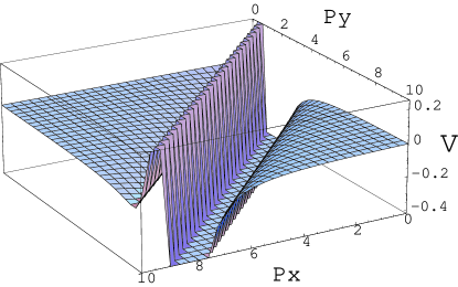
Figure 1: Graph of the potential

The scalar potential (4.12) reduces to the standard (bounded from below) scalar potential $V\propto{\rm Tr}\lfloor{\hskip 0.35pt}\!\!\!\lceil\phi,\bar{\phi}\rfloor{\hskip 0.35pt}\!\!\!\rceil^{2}$ of the undeformed N=2 super-Yang-Mils theory with the $U(2)$ gauge group in the limit $P\to 0$. Equation (4.12) vanishes in the NAC-deformed $U(1)$ gauge group case, when $y=0$, as it should have been expected. Finally, the scalar potential (4.12) reduces to that of eq. (4.4) in the $SU(2)$ limit $x=0$.

The $U(2)$-based potential (4.12) suffers from singularities while it is not positively definite, so that it also implies the absence of a well-defined vacuum in the classical NAC, $U(2)$-based N=2 supersymmetric super-Yang-Mills theory.

5 Conclusion

Our investigation of the NAC-deformed N=2 supersymmetric gauge field theory with a non-simple gauge group $U(2)$ (i.e. with two gauge coupling constants) reveals the rich structure of the effective theory (1.7) after performing the Seiberg-Witen map and the group-theoretical trace. We were able to explicitly calculate the master function governing the component structure of the theory under consideration, as well as its highly non-trivial scalar potential. It should be emphasized that our results are truly non-perturbative in the sense that they include all corrections in the NAC-deformation parameter $P$.

The case of the $U(2)$ gauge group also clearly illustrates the difficulties arising in the efforts to generalize our results to the other gauge groups different from $SU(2)$ and $U(1)$. For instance, in the case of the $SU(3)$ gauge group, the master function is going to depend upon two variables

$$\overline{W}{}^{a}\overline{W}{}^{a}\equiv\delta^{ab}\overline{W}{}^{a}\overline{W}{}^{b}\quad{\rm and}\quad d^{abc}\overline{W}{}^{a}\overline{W}{}^{b}\overline{W}{}^{c}~{}~{},$$

in terms of the two $SU(3)$-invariant symmetric tensors $\delta^{ab}$ and $d^{abc}$, where $a,b,c=1,2,\ldots,8$. By using the structure constants of $SU(3)$ we were able to calculate the leading NAC-contribution to the $SU(3)$ master function,

$${\rm Tr}f(\overline{W}{}^{a}T^{a})=3(\overline{W}{}^{a}\overline{W}{}^{a})-{{27P^{2}}\over{4}}(\overline{W}{}^{a}\overline{W}{}^{a})^{2}+{\cal O}(P^{4})~{},$$

but we faced considerable technical difficulties in calculating the next order terms, not to mention a full non-perturbative answer.

Our considerations in this paper were entirely classical. It is conceivable, however, that the NAC-deformed supersymmetric gauge field theories may even be renormalizable in some sense. So it would be interesting to investigate the role of quantum corrections to eq. (1.7), both in quantum field theory and in superstring theory (e.g., by using geometrical engineering). It is particularly intriguing to know whether quantum corrections can stabilize the classical vacuum.

References

[1] M. R. Douglas and N. A. Nekrasov, Rev. Mod. Phys. 73 (2001)
[hep-th/0106048]
[2] M. Li and Y. S. Wu, Editors,
Physics in Noncommutative World, Rinton Press, New Yersey, 2002
[3] N. Seiberg and E. Witten, JHEP 9909 (1999) 032
[hep-th/9908142];
H. Liu, Nucl. Phys. B614 (2001) 305 [hep-th/0011125];
Y. Okawa and H. Ooguri, Phys. Rev. D64 (2001) 046009 [hep-th/0104036];
Ch. Saemann and M. Wolf, JHEP 0403 (2004) 048 [hep-th/0401147];
D. Mikulovic, JHEP 0405 (2004) 077 [hep-th/0403290]
[4] N. Seiberg, JHEP 0306 (2003) 010 [hep-th/0305248]
[5] L. Brink and J. H. Schwarz, Phys. Lett. B100 (1981) 310;
J. H. Schwarz and P. van Nieuwenhuizen, Lett. Nuovo Cim. 34 (1982) 21;
S. Ferrara and M. A. Lledo, JHEP 0005 (2000) 008 [hep-th/0002084];
D. Klemm, S. Penati and L. Tamassia, Class. Quantum Grav. 20 (2003) 2905
[hep-th/0104190]
[6] J. de Boer, P. A. Grassi and P. van Nieuwenhuizen, Phys.Lett.
B574 (2003) 98 [hep-th/0302078];
A. Imaanpur, JHEP 0309 (2003) 077 [hep-th/0308171];
R. Britto, B. Feng, O. Lunin, S.-J. Rey, JHEP 0307 (2003) 067
[hep-th/0311275]
[7] R. Dijkgraaf and C. Vafa, Nucl. Phys. B644 (2002) 3 and 21;
[hep-th/0206255 and 0207106]; and hep-th/0208048
[8] H. Ooguri and C. Vafa, Adv. Theor. Math. Phys. 7 (2003)
53 and 7 (2004) 405; [hep-th/0302109 and 0303063]
[9] M. Billo, M. Frau, I. Pesando and A. Lerda, JHEP 0405
(2004) 023 [hep-th/0402160]
[10] H. Ooguri and C. Vafa, Mod. Phys. Lett. A5 (1990) 1389;
Nucl. Phys. B361 (1991) 469 ibid.B367 (1991) 83;
J. Bischoff, S. V. Ketov and O. Lechtenfeld, Nucl.Phys. B438
(1995) 373
[hep-th/9406101]
[11] S. J. Gates, Jr., S. V. Ketov and H. Nishino,
Phys.Lett. B297 (1992) 99 [hep-th/9203078]; ibid.B303
(1993) 323 [hep-th/9203081]; Nucl. Phys. B393 (1993) 149 [hep-th/9207042]
[12] T. Araki, L. Ito and A. Ohtsuka, Phys.Lett. B573 (2003)
209 [hep-th/0307076];
E. Ivanov, O. Lechtenfeld, B. Zupnik, JHEP 0402 (2004) 012
[hep-th/0308012];
T. Araki and K. Ito, hep-th/0404250;
S. Ferrara, E. Ivanov, O. Lechtenfeld, E. Sokatchev, B. Zupnik, hep-th/0405049
[13] S. Ferrara and E. Sokatchev, Phys.Lett. B579 (2004) 226
[hep-th/0308021]
[14] S. V. Ketov, Quantum Non-linear Sigma-models,
Springer-Verlag, 2000, Sect. 4.2
[15] S. V. Ketov and S. Sasaki, Phys. Lett. B595 (2004) 530
[hep-th/0404119]
[16] S. V. Ketov and S. Sasaki, hep-th/0405278; to appear in Phys.
Lett. B.