Gravitational collapse and black hole evolution: do holographic black holes eventually “anti-evaporate”?

Abstract

We study the gravitational collapse of compact objects in the Brane-World. We begin by arguing that the regularity of the five-dimensional geodesics does not allow the energy-momentum tensor of matter on the brane to have (step-like) discontinuities, which are instead admitted in the four-dimensional General Relativistic case, and compact sources must therefore have an atmosphere. Under the simplifying assumption that matter is a spherically symmetric cloud of dust without dissipation, we can find the conditions for which the collapsing star generically “evaporates” and approaches the Hawking behavior as the (apparent) horizon is being formed. Subsequently, the apparent horizon evolves into the atmosphere and the back-reaction on the brane metric reduces the evaporation, which continues until the effective energy of the star vanishes. This occurs at a finite radius, and the star afterwards re-expands and “anti-evaporates”. We clarify that the Israel junction conditions across the brane (holographically related to the matter trace anomaly) and the projection of the Weyl tensor on the brane (holographically interpreted as the quantum back-reaction on the brane metric) contribute to the total energy as, respectively, an “anti-evaporation” and an “evaporation” term. Concluding, we comment on the possible effects of dissipation and obtain a new stringent bound for the brane tension.

I Introduction

It is well known that black holes are unstable in four (and higher) dimensions because of the Hawking effect hawking , that is the quantum mechanical production of particles in strong inhomogeneous gravitational fields. It is also well known that such an effect leads (and is deeply linked) to the trace anomaly of the radiation field on the black hole background CF ; birrell . However, for a complete description, the semiclassical Einstein equations should be solved including the back-reaction of the evaporation flux on the metric, which turns out to be an extremely hard task (for a recent attempt to incorporate the effect of the trace anomaly see Ref. vilasi ).

In the context of the Randall-Sundrum (RS) Brane-World (BW) models RS , it was shown in Ref. BGM (see also Ref. kofinas for some recent generalizations) that the collapse of a homogeneous star leads to a non-static exterior, contrary to what happens in four-dimensional General Relativity (GR), and a possible exterior was later found which is radiative dad . If one regards black holes as the natural end state of the collapse, one may conclude that classical black holes in the BW should suffer of the same problem as semiclassical black holes in GR: no static configuration for their exterior might be allowed.

In particular, it was shown in Ref holo , that all known black hole-like metrics on the brane lead to Weyl anomalies with a natural interpretation in the context of the holographic analogy holography . Moreover, such anomalies could be related with an instability, as those metrics do not seem to have the correct weak field expansion in RS (for a discussion of this issue see Ref. gm ). Further, forcing a static exterior, a trace anomaly outside a homogenous and isotropic collapsing star appears which is of the same form, but with opposite sign, as that of semiclassical black holes. This suggested the possibility that black hole metrics which solve the bulk equations with brane boundary conditions, and whose central singularities are located on the brane, genuinely correspond to quantum corrected (semiclassical) black holes on the brane tanaka1 ; fabbri , in the spirit of the holographic principle holography and AdS/CFT conjecture AdSCFT .

We recall that our Universe is a codimension one four-dimensional hypersurface of vacuum energy density $\lambda$ in the BW scenario of Ref. RS . It is hence useful to introduce Gaussian normal coordinates $x^{A}=(x^{\mu},y)$, where $y$ is the extra-dimensional coordinate such that the brane is located at $y=0$ (capitol letters run from $0$ to $4$ and Greek letters from $0$ to $3$). The five-dimensional metric can then be expanded near the brane as maart

$$g^{5}_{AB} = \left.g^{5}_{AB}\right|_{y=0}+2\,\left.K_{AB}\right|_{y=0}\,y+\pounds_{\hat{n}}\left.K_{AB}\right|_{y=0}\,y^{2}$$ (1)

$$+\ldots\ ,$$

where $K_{AB}$ is the extrinsic curvature of the brane, and $\pounds_{\hat{n}}$ the Lie derivative along the unitary four-vector $\hat{n}$ orthogonal to the brane. We also recall that the junction conditions at the brane lead to shiromizu

$$K_{\mu\nu}\sim T_{\mu\nu}-\frac{1}{3}\,\left(T-\lambda\right)\,g_{\mu\nu}\ ,$$ (2)

where $T_{\mu\nu}$ is the stress tensor of the matter localized on the brane, and maart

$$\pounds_{\hat{n}}K_{\mu\nu}\sim{\cal E}_{\mu\nu}+f(T)_{\mu\nu}\ ,$$ (3)

where ${\cal E}_{\mu\nu}$ is the projection of the Weyl tensor on the brane and $f(T)_{\mu\nu}$ a tensor which depends on $T_{\mu\nu}$ and $\lambda$.

The junction conditions in GR israel allow (step-like) discontinuities in the stress tensor (for example, across the surface of a star) keeping the first and second fundamental forms continuous. For thin (Dirac $\delta$-like) surfaces, a step-like discontinuity of the extrinsic curvature orthogonal to the surface is also allowed as long as the metric remains continuous israel . Since a brane in RS is itself a thin surface, it generates an orthogonal discontinuity of the extrinsic curvature in five dimensions as allowed by GR junction conditions. However, any discontinuities in the matter stress tensor on the brane would induce discontinuities in the extrinsic curvature (2) which are tangential to the brane and would therefore appear in the five-dimensional metric (1). Such discontinuities of the metric are not allowed by the regularity of five-dimensional geodesics. Moreover, because of the second order term in Eq. (1) and considering Eq. (3), we can not allow the projected Weyl tensor to be discontinuous on the brane either . One can understand the above regularity requirement by considering that, in a microscopic description of the BW, matter should be smooth along the fifth dimension, yet localized on the brane (say, within a width of order $\lambda^{-1/2}$, in units $G=c=1$ g2 ). In any such description, the continuity of five-dimensional geodesics must then hold and, in order to build a physical model of a star, one has to smooth both the matter stress tensor and the projected Weyl tensor across the surface of the star along the brane.

We shall employ the effective four-dimensional (hydrodynamical) equations of Refs. maart ; shiromizu in our analysis. In general, such equations cannot determine the brane metric uniquely unless one also knows the bulk geometry. However, if the system enjoys enough symmetries, the effective four-dimensional equations are closed and can thus give some insight about the bulk . In particular, we shall show that, under the simplifying assumption that the heat flow is always negligible (no dissipation), the knowledge of the full five-dimensional dynamics of the most central region of the collapsing star renders the whole system “physically closed” when the energy density of the star is much smaller than the brane tension. By physically closed we mean that the evolution of the system is uniquely determined upon further requiring that the four-dimensional metric become Minkowski in the limit of zero energy density and at spatial infinity (asymptotic flatness). Although considering a non-dissipative model appears restrictive, we would like to remark that the same kind of models in GR leads to paradigmatic examples of black hole formation, beside the fact that this is the only case which can be solved analytically.

The Oppenheimer-Snyder (OS) model in GR OS yields the simplest description of how black holes could form from collapsing stars. It has however been shown that this kind of model is not viable in the RS scenario BGM since, if one forces a static exterior outside homogeneous and isotropic stars, BW effects produce an effective “energy surplus” which is encoded by a positive curvature in such an exterior and which cannot be generated by any bulk back-reaction. Hence, we expect that this excess energy will be released via a mechanism that leads to a loss of mass from the star. Although the positive curvature in the exterior has no GR description, it can also be obtained from quantum computations CF   but with the opposite sign. The sign mismatch between classical and quantum results might be reconciled on recalling that the classical anomaly is due to an effective potential energy at the boundary of the star which must be released in order to have an exterior compatible with the junction conditions phd . It might therefore be possible to change the sign of the anomaly just considering that the energy surplus should be converted into an effective negative flux of energy from the boundary of the star.

In order to do so, we shall employ a Tolman geometry tolman for the brane star, as it is the only spherically symmetric metric which does not allow dissipation of energy across the shells of the collapsing star, and the Hawking radiation can then be interpreted as the emission of gravitons into the bulk. In fact, it turns out that the propagation of CFT modes in four dimensions is consistently described by this mechanism according to the AdS/CFT correspondence tanaka1 . Moreover, we require the continuity of the Weyl and energy-momentum tensors as discussed above, and we shall show that a Tolman brane metric corresponds to a general five-dimensional diagonal metric with spherically symmetric slices .

We shall divide the domain of the star into three regions: I) the “core”, where most of the energy of the star is concentrated; II) a “transition region”, which connects the core with a tail and finally III) a “tail”, where the energy density approaches zero. The tail and transition region together form an “atmosphere” of the sort that is usually employed in numerical simulations of the gravitational collapse (see, e.g. Ref. rezzolla ). The core is taken homogeneous and isotropic (OS-like) for several reasons. Firstly, in order to consider a minimal modification with respect to the OS model in GR. Secondly, the OS core corresponds to an exact five-dimensional solution langlois and reproduces the correct Weyl anomaly of quantum field theory on the Schwarzschild background CF ; birrell , thus making the holographic interpretation clearer. Our main results will then be that, in this case, the total energy of the system is conserved  and that the collapsing star “evaporates” until the core experiences a “rebound” in the high energy regime (when its energy density is comparable with $\lambda$), after which the whole system “anti-evaporates”. Moreover, we can find a range of parameters for which the minimum radius of the collapsing core is larger than the AdS length (which sets the scale of Quantum Gravity in the BW), thus further supporting the qualitative behavior we obtain.

In Section II, we shall briefly review a simple holographic interpretation of the Hawking radiation in the BW. In Section III, we shall build a physical model of the Tolman type that converges to the OS model in the GR limit and show that BW corrections lead to an emission of energy from the star and a bounce of the core (see also Appendix A). In Section IV, we shall analyze in details how the (apparent) horizon forms and physical quantities related to it, such as the outer trace anomaly, which will then be interpreted in terms of the BW corrections coming from the brane junction conditions. In section V we shall discuss the possible effects of dissipation. We shall finally comment on our results in Section VI.

In the following, we shall use geometrical units with $G=c=1$ and mostly positive metric signature.

II Simple holographic picture

Before trying to “cure” the Weyl anomaly, let us have a closer look at the features of the effective energy surplus in the exterior of the star discovered in Ref. BGM . We first note that, as pointed out by different authors holo ; fabbri ; phd , the energy surplus reproduces the absolute value of the quantum Weyl anomaly computed on a Schwarzschild background CF , which is the unique exterior of a spherical star in GR. More precisely, in static coordinates one has, outside of the star,

$$R^{\mu}_{\ \mu}=\frac{9}{2\,\pi\,\lambda}\,\frac{M^{2}}{R^{6}}\ ,$$ (4)

where $R^{\mu}_{\ \mu}$ is the Ricci scalar, $M$ the physical mass of the star , and $R$ the Schwarzschild radial coordinate. As remarked in Ref. fabbri , the holographic interpretation for such a contribution cannot be of the exact AdS/CFT kind, because both classical black holes on the brane and semiclassical black holes in GR correspond to strong deviation from AdS and CFT (see also Ref. holo ). We shall indeed show that we cannot reproduce the evaporation process if the bulk is simply AdS (i.e. with zero Weyl tensor).

As a first step, we shall show that, if a black hole is formed from matter collapsing in the BW, the area of its horizon (to first order in $\lambda^{-1}$ and for a short time after its formation) follows the evaporation law for semiclassical black holes hawking . In particular, we will see that the horizon evaporates provided the Weyl contribution is dominant, and we may therefore assert that the BW collapse gives, to first order in $\lambda^{-1}$ and for some five-dimensional geometries, a good description of the first order quantum processes related to it. Let us also note that quantum calculations in Refs. hawking ; CF are performed in adiabatic approximation, that is, in some sense, to first order in the back-reaction parameter of the quantum theory.

Following Ref. BGM , a unique static geometry which matches a collapsing homogeneous and isotropic cloud of dust, has a Schwarzschild-like metric with mass function

$$M=M_{\rm S}+\frac{1}{\lambda}\,m(R)\ ,$$ (5)

where $M_{\rm S}$ is the usual ADM contribution (see Section III for more details) and

$$m(R)=\frac{3\,M_{\rm S}^{2}}{8\,\pi\,R^{3}}-\frac{9\,\mu}{32\,\pi\,R}\ ,$$ (6)

where, in a cosmological background, the constant $\mu$ is related with the mass of a black hole sitting in the bulk bh and we set the effective four-dimensional cosmological constant to zero (since we are just interested in BW effects on asymptotically flat branes).

We denote with $R_{0}=R_{0}(\tau)$ the radius of the collapsing object which depends on the proper time $\tau$. The geodesic equation of motion in the Schwarzschild-like space-time determines $R_{0}$ according to 

$$\dot{R}_{0}^{2}=\frac{2\,M}{R_{0}}=\frac{2\,M_{\rm S}}{R_{0}}+\frac{3}{4\,\pi\,\lambda\,R_{0}^{2}}\,\left(\frac{M_{\rm S}^{2}}{R_{0}^{2}}-\frac{3}{4}\,\mu\right)\ ,$$ (7)

in which we have selected the case corresponding to zero initial velocity for infinite initial radius. We can now see how the mass function is changing when the surface of the star crosses its own horizon, that is at the time $\tau_{\rm H}$ when $R_{0}(\tau_{\rm H})\equiv R_{\rm H}=2\,M_{\rm H}\equiv 2\,M(\tau_{\rm H})=2\,M_{\rm S}+2\,m(R_{\rm H})/\lambda$  and $\dot{R}_{\rm H}=-1$. Let us define the surface area of the evolving “apparent horizon” as $A_{\rm AH}=16\,\pi\,M^{2}(\tau)$, for which Eq. (5) gives

$$\dot{A}_{\rm AH}=\frac{9}{4\,\lambda}\,\left[\mu-\left(\frac{M_{\rm S}}{M}\right)^{2}\right]\,\frac{\dot{R}}{M}\ .$$ (8)

Considering that $M_{S}/M\simeq 1$ to first order in $\lambda^{-1}$, at the time $\tau=\tau_{\rm H}$, we then have

$$\dot{A}_{\rm AH}\simeq-\frac{9}{4\,\lambda}\,\frac{\mu-1}{M_{\rm H}}\ ,$$ (9a)

or

$$\dot{M}_{\rm H}\simeq-\frac{9}{128\,\pi\,\lambda}\,\frac{\mu-1}{M_{\rm H}^{2}}\ .$$ (9b)

The collapse therefore leads to a negative flux of energy when the boundary of the star approaches its horizon, as expected for the Hawking evaporation, if $\mu>1$.

Since a positive $\mu$ generally corresponds to a reinforcement of the localization of gravity in RS maa2 , we can assert that an OS region mainly evaporates into gravitational waves propagating on the brane. We shall however see that, for a consistent model of collapsing star with continuous density, the sign of the Weyl energy changes from the interior to the exterior of the star, so that the evaporation actually ejects energy off the brane via gravitational waves (as suggested in Ref. tanaka1 ).

So far, we have not considered any back-reaction on the brane metric, and the same flux (9b) will reasonably be seen by a distant observer for whom $\partial_{\tau}$ asymptotically becomes a time-like Killing vector. However, the surplus energy must be released, since no BW or GR model can explain the Weyl anomaly, and this directly implies that Eq. (9b) probably holds only for a short time about the formation of the horizon, as suggested in BGM . We shall indeed show that this is the case.

III Gravitational collapse on the brane

In this section we will study a continuous model for the gravitational collapse. In order to see the difference with respect to the OS-like model studied in Ref. BGM , we consider a Tolman-like model with a central OS core. The star is therefore described as a cloud of dust with falling off continuous density and no sharp boundary. The classical four-dimensional behavior will be recovered in the limit of negligible star density (with respect to the brane vacuum energy density $\lambda$).

III.1 General framework

Following Ref. maart , we can rewrite the BW effective four-dimensional Einstein equations with vanishing cosmological constant on the brane as

$$G_{\mu\nu}=8\,\pi\,T_{\mu\nu}^{\rm eff}\ .$$ (10)

Here we have

$$T_{\mu\nu}^{\rm eff}=\rho^{\rm eff}\,u_{\mu}\,u_{\nu}+p^{\rm eff}\,h_{\mu\nu}+q^{\rm eff}_{(\mu}\,u_{\nu)}+\pi^{\rm eff}_{\mu\nu}\ ,$$ (11)

where $u^{\mu}$ is the unit four-velocity of matter ($u^{\mu}u_{\mu}=-1$), $h_{\mu\nu}$ the space-like metric that projects orthogonally to $u^{\mu}$ ($h_{\mu\nu}=g_{\mu\nu}+u_{\mu}u_{\nu}$) and $\pi^{\rm eff}_{\mu\nu}$ an anisotropic tensor.

For an isotropic perfect fluid, BW corrections to GR are described by the effective quantities maart

$$\rho^{\rm eff} = \rho\,\left(1+\frac{\rho}{2\,\lambda}+\frac{\cal U}{\rho}\right)$$ (12a)

$$p^{\rm eff} = p+\frac{\rho}{2\,\lambda}\left(2\,p+\rho\right)+\frac{\cal U}{3}$$ (12b)

$$q^{\rm eff}_{\mu} = Q_{\mu}$$ (12c)

$$\pi^{\rm eff}_{\mu\nu} = \Pi_{\mu\nu}\ ,$$ (12d)

where $\rho$ and $p$ are the (“bare”) energy density and pressure of matter. We also employed the following decomposition of the projection of the Weyl tensor on the brane

$$-{\frac{1}{8\pi}}\,{\cal E}_{\mu\nu} = {\cal U}\,\left(u_{\mu}\,u_{\nu}+\frac{1}{3}\,h_{\mu\nu}\right)$$ (13)

$$+{Q_{\mu}}\,u_{\nu}+{Q_{\nu}}\,u_{\mu}+\Pi_{\mu\nu}\ ,$$

corresponding to an effective “dark” radiation on the brane with energy density $\cal U$, pressure ${\cal U}/3$, momentum density $Q_{\mu}$ and anisotropic stress ${\Pi}_{\mu\nu}$. Note that non-local bulk effects can contribute to effective imperfect fluid terms even when brane matter is a perfect fluid.

Bianchi identities supplied by the junction conditions produce two kinds of conservation equations maart :

1. Local conservation equations (LCE):

   $$\dot{\rho}+\Theta\,\left(\rho+p\right)=0$$ (14a)

   $$\mbox{D}_{a}p+\left(\rho+p\right)\,A_{a}=0\ ;$$ (14b)

2. Non-local conservation equations (NLCE’s):

   $$\!\!\!\!\!\!\dot{{\cal U}}+\frac{4}{3}\,\Theta\,{{\cal U}}+\mbox{D}^{a}Q_{a}+2\,A^{a}\,Q_{a}+\sigma^{ab}\,\Pi_{ab}=0$$ (15a)

   $$\!\!\!\!\!\!\dot{Q}_{a}+{\frac{4}{3}}\,\Theta\,Q_{a}+{\frac{1}{3}}\,\mbox{D}_{a}{{\cal U}}+\frac{4}{3}\,{{\cal U}}\,A_{a}+\mbox{D}^{b}\Pi_{ab}$$

   $$+A^{b}\,\Pi_{ab}+\sigma_{a}^{\ b}\,Q_{b}-\omega_{a}^{\ b}\,Q_{b}=-\frac{\rho+p}{\lambda}\,\mbox{D}_{a}\rho\ ,$$ (15b)

where $D_{a}$ is the spatially projected derivative (defined by $D_{a}S^{b...}{}_{...c}=h^{e}{}_{a}h^{b}{}_{f}...h^{g}{}_{c}\nabla_{e}S^{f...}{}_{...g}$ for $a=1,\ 2,\ 3$), $\Theta=\nabla^{\alpha}u_{\alpha}$ the volume expansion, $\dot{S}^{a...}{}_{...b}=u^{\alpha}\,\nabla_{\alpha}S^{a...}{}_{...b}$ the proper time derivative, $A_{a}=\dot{u}_{a}$ the acceleration, $\sigma_{ab}=D_{(a}u_{b)}-(\Theta/3)\,h_{ab}$ the (traceless) shear, and $\omega_{ab}=-D_{[a}u_{b]}$ the vorticity.

III.2 Spherically symmetric dust

For the case with zero pressure ($p=0$), that is dust on the brane, the quantities in Eqs. (12a), (12b) and (12d) reduce to

$$\rho^{\rm eff} = \rho\,\left(1+\frac{\rho}{2\,\lambda}\right)+{\cal U}$$ (16a)

$$p^{\rm eff} = \frac{\rho^{2}}{2\,\lambda}+\frac{\cal U}{3}$$ (16b)

$$\pi^{\rm eff}_{\mu\nu} = \Pi_{\mu\nu}\ .$$ (16c)

Provided the matter density $\rho$ does not vanish in the region of interest, one can use comoving coordinates in which $u^{\alpha}=(-1,0,0,0)$.

In the following, we will only consider the class of five-dimensional metrics which are diagonal (sufficiently close to the brane at $y=0$) and spherically symmetric on the brane. In Gaussian normal coordinates, one can always write a bulk metric which is spherically symmetric on the brane as

$$\!\!\!\mbox{{\rm d}}s^{2} \!\!=\!\! -N^{2}(\tau,r,y)\,\mbox{{\rm d}}\tau^{2}+A^{2}(\tau,r,y)\,\mbox{{\rm d}}r^{2}$$ (17)

$$+2\,B(\tau,r,y)\,\mbox{{\rm d}}t\,\mbox{{\rm d}}r+R^{2}(\tau,r,y)\,\mbox{{\rm d}}\Omega^{2}$$

$$+\mbox{{\rm d}}y^{2}\ .$$

Upon using the restricted freedom to change the four-dimensional coordinates on the brane, one can always set $B(\tau,r,0^{+})=0$ LL , so that the brane metric reads

$$\left.\mbox{{\rm d}}s^{2}\right|_{y=0^{+}} = -N^{2}(\tau,r,0^{+})\,\mbox{{\rm d}}\tau^{2}+A^{2}(\tau,r,0^{+})\,\mbox{{\rm d}}r^{2}$$ (18)

$$+R^{2}(\tau,r,0^{+})\,\mbox{{\rm d}}\Omega^{2}\ .$$

Since we just consider dust as brane matter, from the junction conditions at the brane maart , we also obtain

$$0=K_{\tau r}^{+}(\tau,r)\equiv\left.\frac{1}{2}\,\frac{\partial g_{\tau r}}{\partial y}\right|_{y=0^{+}}=\left.\frac{\partial B}{\partial y}\right|_{y=0^{+}}=0\ .$$ (19)

Using the above result together with the bulk symmetry $Z_{2}$ with respect to the brane, we have $B(\tau,r,y)=y^{2}\,\left[V(\tau,r)+{\mathcal{O}}(y)\right]$. Since the Weyl energy flux is related to $B$ by

$$Q_{a}\sim\left.\frac{\partial^{2}B}{\partial y^{2}}\right|_{y=0^{+}}$$ (20)

one finds that $Q_{a}$ vanishes if $V(\tau,r)=0$, which is in fact what we are assuming. The coefficient $g_{\tau r}$ then vanishes fast enough on the brane so that, from the five-dimensional Einstein equations

$${}^{(5)}G_{AB}=-\Lambda\,g_{AB}\ ,$$ (21)

in the limit $y\to 0^{+}$, one obtains the condition 

$$0=\!\!\left.{}^{(5)}\!G_{\tau r}\right|_{y=0^{+}}\!\!\!\!=\left.\frac{2}{NA}\,\left(\frac{\dot{A}}{A}\,\frac{R^{\prime}}{R}+\frac{\dot{R}}{R}\,\frac{N^{\prime}}{N}-\frac{\dot{R}^{\prime}}{R}\right)\right|_{y=0^{+}}\!\!\!,$$ (22)

where a prime denotes $\partial_{r}$ and a dot $\partial_{\tau}$. Since our matter is pressureless, we can work in the proper time gauge $N(\tau,r,0^{+})=1$ LL and, using the residual gauge freedom in defining the radial coordinate $r$, we obtain

$$A(\tau,r,0^{+})=R^{\prime}(\tau,r,0^{+})\ .$$ (23)

This relation implies a Tolman geometry on the brane 

$$\mbox{{\rm d}}s^{2}=-\mbox{{\rm d}}\tau^{2}+\left(R^{\prime}\right)^{2}\,\mbox{{\rm d}}r^{2}+R^{2}\,\mbox{{\rm d}}\Omega^{2}\ ,$$ (24)

where $R=R(\tau,r)$ is a (generally non-separable) function of $\tau$ and $r$ such that $4\,\pi\,R^{2}(\tau,r)$ equals the surface area of the shell comoving with dust particles located at the coordinate position $r$ at the proper time $\tau$.

With the above symmetries, the vorticity, the acceleration and the Weyl energy flux vanish, $\omega_{a}=A_{a}=Q_{a}=0$, and we obtain the simplified LCE

$$\partial_{\tau}{\rho}+\Theta\,\rho=0\ ,$$ (25)

and NLCE’s

$$\partial_{\tau}{{\cal U}}+{\frac{4}{3}}\,\Theta\,{{\cal U}}+\sigma^{ab}\,\Pi_{ab}=0$$ (26a)

$${\frac{1}{3}}\,D_{a}{{\cal U}}+D^{b}\Pi_{ab}=-\frac{\rho}{\lambda}\,D_{a}\rho\ .$$ (26b)

The volume expansion is also easily computed as

$$\Theta=\partial_{\tau}\left[\ln\left(R^{2}\,\partial_{r}R\right)\right]=\frac{\partial_{\tau}\partial_{r}\left(R^{3}\right)}{\partial_{r}\left(R^{3}\right)}\ ,$$ (27)

and for the shear one finds

$$\sigma_{ab}=\frac{1}{2}\,\partial_{\tau}h_{ab}-\frac{\Theta}{3}\,h_{ab}\ ,$$ (28)

where $h_{ab}=g_{ab}$ is the spatial part of the metric (24).

By symmetry, we expect that the anisotropic pressure tensor is diagonal and isotropic in the angular directions. Moreover, considering that $\Pi^{\alpha}{}_{\alpha}=0$ we have, in such adapted coordinates,

$$\Pi^{a}_{\ b}=\mbox{diag}\,\left(\frac{2}{3}\,\Pi,-\frac{1}{3}\,\Pi,-\frac{1}{3}\,\Pi\right)\ ,$$ (29)

and

$$\sigma^{ab}\,\Pi_{ab}=\frac{1}{2}\,\partial_{\tau}g_{ab}\,\Pi^{ab}=-\frac{2}{3}\,\Pi\,\left(\frac{\partial_{\tau}R}{R}-\frac{\partial_{\tau}\partial_{r}R}{\partial_{r}R}\right)\ ,$$ (30)

which vanishes in the OS background (homogeneous and isotropic space-time) for which

$$R(\tau,r)=g(r)\,X(\tau)\ .$$ (31)

We then see that the NLCE’s become

$$\!\!\!\!\!\!\!\!\dot{\cal U}+\frac{4}{3}\,\left[\frac{\dot{R}}{R}\,\left(2\,{\cal U}-\frac{\Pi}{2}\right)+\frac{\dot{R}^{\prime}}{R^{\prime}}\,\left({\cal U}+\frac{\Pi}{2}\right)\right]=0$$ (32a)

$$\!\!\!\!\!\!\!\!\frac{1}{3}\,{\cal U}^{\prime}+\frac{2}{3}\,\left[\Pi^{\prime}+3\,\frac{R^{\prime}}{R}\,\Pi\right]=-\frac{\rho}{\lambda}\,\rho^{\prime}\ .$$ (32b)

The system of NLCE’s is in general not closed, since we do not have an evolution equation for $\Pi$. However, for a sufficiently large physical radius $R$, the knowledge of $\Pi$ in an extended spatial region together with the asymptotic flatness and the continuity of ${\cal E}_{\mu\nu}$ make that system closed. Let us remark that this also happens in the cosmological perturbative scenario in which one considers large-scale evolution of the Weyl tensor bruni .

The LCE (25) integrated over the spatial volume $\sqrt{h}\,\mbox{{\rm d}}r\,\mbox{{\rm d}}\theta\,\mbox{{\rm d}}\phi=\sin\theta/3\,\partial_{r}(R^{3})\,\mbox{{\rm d}}r\,\mbox{{\rm d}}\theta\,\mbox{{\rm d}}\phi$ implies

$$\partial_{\tau}m_{\rho}=0\ ,$$ (33)

where we have introduced the “bare” mass function

$$m_{\rho}(r)\equiv\frac{4\,\pi}{3}\,\int^{r}_{0}\rho(\tau,x)\,\partial_{x}\left(R^{3}(\tau,x)\right)\,\mbox{{\rm d}}x\ ,$$ (34)

or, equivalently,

$$\rho(\tau,r)=\frac{m_{\rho}^{\prime}}{4\,\pi\,R^{2}\,R^{\prime}}\ .$$ (35)

The meaning of Eq. (33) is that, since we have chosen a comoving reference frame and $p=0$, the “bare” energy contained within a sphere of fixed coordinate radius $r$ cannot change in time, although the physical radius $R(\tau,r)$ of such a sphere decreases during the collapse.

We can now consider the $(\tau,\tau)$ Einstein equation,

$$G^{\tau}_{\ \tau}=-\frac{(\dot{R}^{2}\,R)^{\prime}}{R^{2}\,R^{\prime}}=-8\,\pi\,\rho^{\rm eff}\ ,$$ (36)

which yields the equation of motion

$$\dot{R}^{2}(\tau,r)=\frac{2\,M(\tau,r)+F(\tau)}{R(\tau,r)}\ ,$$ (37)

where we have introduced the “effective” mass

$$M(\tau,r)=\frac{4\,\pi}{3}\,\int^{r}_{0}\rho^{\rm eff}(\tau,x)\,\partial_{x}\left(R^{3}(\tau,x)\right)\,\mbox{{\rm d}}x\ .$$ (38)

Since we want a flat brane for $M=0$ [moreover, the center of the star is at rest, $\dot{R}(\tau,0)=0$], it must be $F(\tau)=0$ and we finally obtain

$$\dot{R}^{2}(\tau,r)=\frac{2\,M(\tau,r)}{R(\tau,r)}\ .$$ (39)

Let us note that the effective mass is not constant in general. In fact,

$$\!\!\!\!\!\!\dot{M}(\tau,r) = \frac{4\,\pi}{3}\,\partial_{\tau}\int^{r}_{0}\rho^{\rm eff}\,\partial_{x}(R^{3})\,\mbox{{\rm d}}x$$ (40)

$$= \frac{4\,\pi}{3}\,\int^{r}_{0}\partial_{\tau}\left[\left(\frac{\rho^{2}}{2\,\lambda}+{\cal U}\right)\,\partial_{x}\left(R^{3}\right)\right]\,\mbox{{\rm d}}x\ .$$

For the particular case $\Pi=0$, one then obtains

$$\dot{M}(\tau,r)=-\frac{4\,\pi}{3}\,\int^{r}_{0}\left(\frac{\rho^{2}}{2\,\lambda}+\frac{{\cal U}}{3}\right)\,\partial_{x}\partial_{\tau}\left(R^{3}\right)\,\mbox{{\rm d}}x\ ,$$ (41)

where we have used both the LCE and the first NLCE.

A very important result which follows from the LCE and NLCE’s is that, if the brane metric is asymptotically flat, the anisotropic stress $\Pi\not=0$ whenever $\dot{\rho}^{\prime}\neq 0$. We can prove it by showing that $\Pi=0$ is not compatible with asymptotic flatness and the LCE and NLCE’s. On combining Eq. (32a) with Eq. (25) for $\Pi=0$, we obtain

$${\cal U}=U(r)\,\rho^{4/3}\ ,$$ (42)

where $U(r)$ is a time-independent integration function. From Eq. (32b) with $\Pi=0$, one instead obtains

$${\cal U}=-\frac{3\,\rho^{2}}{2\,\lambda}+F(\tau)\ ,$$ (43)

$F(\tau)$ being a spatially-constant integration function. Asymptotic flatness requires that

$$\lim_{r\to\infty}{\cal U}(\tau,r)=\lim_{r\to\infty}\rho(\tau,r)=0\ ,\ \ \ \ \forall\,\tau\ ,$$ (44)

which implies $F(\tau)=0$. On now combining Eq. (42) with Eq. (43), we get the relation

$$U(r)=-\frac{3\,\rho^{2/3}}{2\,\lambda}\ ,$$ (45)

which obviously contradicts the assumption $\dot{\rho}^{\prime}\neq 0$. This implies that, for a continuous distribution of dust for which $\dot{\rho}^{\prime}\not=0$, one must have $\Pi\not=0$. This result supports the holographic interpretation as it resembles very much a property of the renormalized quantum stress tensor on the Schwarzschild background CF .

III.3 The model

As mentioned before, we shall divide the star in three regions  (see Fig. 1 for a qualitative picture):

I    

: the “core” ($0\leq r<r_{0}$), where $\rho^{\prime}=0$ and one has an OS OS behavior;

II  

: the “transition region” ($r_{0}<r<r_{\rm s}$), with Tolman tolman behavior due to $\rho\,\rho^{\prime}$ being non-negligible;

III

: the “tail” ($r>r_{\rm s}$), with $\rho\,\rho^{\prime}\simeq 0$.

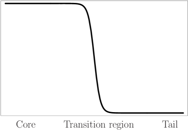
Figure 1: Density profile.

Moreover, we define the dimensionless parameter

$$\epsilon\equiv{\rho_{0}/\lambda}\ ,$$ (46)

where $\rho_{0}\equiv\rho(\tau=0,r=0)$ is the initial core density. Such a parameter is assumed small, since the system is initially in a low energy regime (from the BW point of view) and relevant quantities can thus be expanded in powers of $\epsilon$ for sufficiently short times (or sufficiently large distance from the core).

A basic feature of both Tolman and OS models in four-dimensional GR is that the bare mass function at fixed comoving radius is constant in time and remains well defined during all the collapse. Therefore, dust shells of different comoving radius move along geodesics solely determined by the inner geometry and reach the central singularity ($R=0$) at increasing proper times (Tolman model) or at the same proper time (OS model). In the former case one can have an enlarging apparent horizon , while in the latter just an event horizon forms at the star surface LL .

In the BW, the role of the bare mass is taken by the effective mass $M$ of Eq. (38), which will be shown to diverge whenever $R\to 0$, thus making the whole four-dimensional space-time singular. To avoid this case, which is mathematically admissible but physically unlikely, one has to include a sufficiently negative contribution to the mass coming from the projected Weyl tensor. As we discussed in Section II, this will generate an Hawking flux near the forming horizon, and we shall further show that the effective mass completely evaporates at a finite star radius, after which the collapse changes to a re-expansion (or “anti-evaporation” process). This case of BW collapse and rebound cannot be related to the GR behavior perturbatively (in $\epsilon\sim\lambda^{-1}$), since none of the shells reach $R=0$, but we incidentally note that it seems in agreement with the uncertainty principle of quantum mechanics . In fact, a “bounce” in the trajectories of the collapsing matter caused by quantum gravitational fluctuations had already been found in an improved semiclassical analysis of the OS model impBO .

III.3.1 The core

We first recall that the bulk solution which corresponds to the OS core of the star is perfectly regular in five dimensions far from the space-time singularity langlois . Further, since $\rho^{\prime}=0$, the system of relevant equations is now closed. In fact, we have $\Pi=0$, and the NLCE’s reduce to the one equation

$$\dot{{\cal U}}+\frac{4}{3}\,\Theta\,{{\cal U}}=0\ ,$$ (47)

which is solved by

$${\cal U}=-\frac{27\,\mu\,r^{4}\,\epsilon}{128\,\pi^{2}\,r_{0}^{4}\,\rho_{0}\,R^{4}}\ ,$$ (48)

where $\mu$ is a constant.

The physical radius $R$ can in general be written in the factorized form (31) and the coordinate $r$ can be so chosen that

$$g(r)=\left(\frac{9}{2}\,M_{\rm S}\right)^{1/3}\,\frac{r}{r_{0}}\ ,$$ (49)

in which $M_{\rm S}$ is the total bare mass of the OS core. The effective mass (38) is then given inside the core by

$$\!\!\!\!\!\!\!M(\tau,r) \!\!=\!\! M_{\rm S}\left(\frac{r}{r_{0}}\right)^{3}$$ (50)

$$+\frac{9\,\epsilon}{32\,\pi\,\rho_{0}}\left(\frac{r}{r_{0}}\right)^{4}\left[\frac{(2\,M_{\rm S})^{2}}{3\,R^{3}}\left(\frac{r}{r_{0}}\right)^{2}-\frac{\mu}{R}\right]\ ,$$

where the first term in the r.h.s. is the usual bare mass and the remainder represents the BW correction.

The above effective mass would diverge for $R\to 0$ (this also occurs for a general Tolman core, see Appendix A). The point $R=0$ is the usual central singularity, which is harmless (at least when covered by an horizon) in four-dimensional GR, since the bare mass is constant and finite. In the present case, however, the diverging effective energy makes the whole space-time singular. In order to see this, let $T$ be the proper time at which the OS core hits the singularity. From the equation of motion (39) one has

$$\left.R\,\dot{R}^{2}\right|_{r>r_{0}}=2\,M(T,r_{0})+8\,\pi\,\int_{r_{0}}^{r}\rho^{\rm eff}\,R^{2}\,R^{\prime}\,\mbox{{\rm d}}x\ .$$ (51)

Since $M(\tau\to T,r_{0})\to\infty$, either the second term in the r.h.s. is finite and the total effective mass diverges at any $r>r_{0}$, thus making the whole exterior singular, or it equals $-M(T,r_{0})+f(r)$, with $f(r)$ a regular function, in order to compensate for the diverging core energy. In the latter case, the Weyl energy becomes everywhere infinitely large and negative and, since $G^{a}_{\ a}\sim{\cal U}$, the whole four-dimensional Einstein tensor is singular. Although such singular evolutions appear mathematically allowed by the equations, in the following we shall not consider them since, from the BW point of view, either they predict a catastrophic end of the Universe induced by astrophysical events or, more reasonably, they suggest that a more fundamental model must be used. However, in the latter case we expect for large black holes that a huge energy flux would be emitted towards infinity well before the OS boundary approaches the Planck length. This, of course, would be ruled out by astronomical observations. From the holographic perspective we are interested in here, only the non-singular solution is relevant. In fact, it is only in this case that the star continuously “evaporates” (before the bouncing) by emitting a Hawking-like energy flux at the moment when the OS horizon forms, as we shall see later. Moreover the bouncing solution seems to be compatible with some proposal for the quantum black hole formation Haw ; impBO .

In order to avoid the singular cases, one must have $\mu$ positive and large enough so that each shell will bounce back after reaching a minimum radius where the corresponding effective mass vanishes . The Weyl tensor, holographically interpreted as the quantum back-reaction on the brane metric (see phd and References therein), then contributes the “evaporation” term proportional to $\mu$ in Eq. (50), which dominates at relatively low energies; whereas, the BW correction to the matter stress tensor, holographically interpreted as the matter quantum trace anomaly tanaka1 , yields the “anti-evaporating” term proportional to $M_{S}^{2}$ in Eq. (50), which increases with the energy.

Upon inserting the effective mass (50) in the equation of motion (39), one obtains an equation for $X(\tau)$,

$$\dot{X}^{2} = \frac{4}{9\,X}+\frac{\epsilon}{27\,\pi\,\rho_{0}\,X^{4}}-\frac{6^{1/3}\,\epsilon\,\mu}{24\,\pi\,\rho_{0}\,M_{\rm S}^{4/3}\,X^{2}}$$ (52)

$$\equiv -V(X)\ ,$$

in which there is no dependence on $r$. This shows that the system remains “rigid” through the bounce: no shell crossing occurs and all shells reach their minimum radius at the same proper time. Like for the classical OS model, it is thus sufficient to consider the evolution of the core surface at $r=r_{0}$ and we correspondingly define $M_{0}(\tau)=M(\tau,r_{0})$ and $R_{0}(\tau)=R(\tau,r_{0})$.

$V$ $X$

Figure 2: Qualitative behavior of the shells and core potential for $\mu>\mu_{\rm c}$ (solid line) and $\mu<\mu_{\rm c}$ (dashed line). For $\mu=\mu_{\rm c}$ (dotted line), the peak of $V$ equals the shells energy $E=0$.

$\tau$
(a)
$\tau$
(b)

Figure 3: Typical evolutions of the core radius $R_{0}(\tau)/R_{0}(0)$ (solid line) and effective mass $M_{0}(\tau)/M_{0}(0)$ (dashed line) for $\mu<\mu_{\rm c}$ (a) and for $\mu>\mu_{\rm c}$ (b). Units are arbitrary.

From the form of the potential $V$ in Eq. (52) (see also Fig. 2), one can see that the term proportional to $\mu$ behaves as a repulsive (angular momentum-like) force and the bounce occurs whenever there is a positive peak (since the energy of collapsing shells $E=0$ for our choice of initial conditions). There will in general exist a critical value $\mu_{\rm c}=\mu_{\rm c}(M_{\rm S},\rho_{0},\epsilon)$ such that one has the bounce for $\mu>\mu_{\rm c}$, otherwise $R_{0}\to 0$ and $M_{0}$ diverges. For $\mu=\mu_{\rm c}$ the two turning points of the potential coincide and the shells would take an infinite proper time to reach the minimum radius (of course, this would only occur if one neglected any perturbations, and we shall not further consider this special case). In Fig. 3 we display a typical trajectory of $R_{0}$, along with the corresponding time evolution of the core effective mass $M_{0}$, for $\mu<\mu_{\rm c}$ in panel (a) and for $\mu>\mu_{\rm c}$ in (b). In the latter case, after the core surface has reached the point of zero effective mass, it will bounce back transforming the whole collapse into an “explosion”, which evolves as in (b) with the time reversed. Although we are not able to describe the dynamics of the atmosphere at very high energies (e.g. around the bounce) by means of our perturbative analysis, on considering that the continuity of the total energy-momentum tensor would be spoiled if the shells crossed , one finds that all the shells (both in the core and the atmosphere) must begin to re-expand. Because of energy conservation at infinity, this “reversal of motion” in the atmosphere would generate an instantaneous distributional (Dirac $\delta$-like) term in the Ricci scalar, as it was also found in a semiclassical treatment of bouncing solutions Russo . Such a singularity in turn means that a detailed description of the collisions between matter shells at fixed $r$ inside the atmosphere and with the core must be taken into account at that point. A microscopic description of the shells goes however beyond the scope of the present paper and we just wish to make a remark. In practice, during the bounce the collisionless description of dust must be relaxed by introducing an effective short distance potential which results in an effective equation of state for the atmosphere. Since our system is non-dissipative by construction, the scatterings should be completely elastic and the equation of state of the polytropic type (see, e.g. Ref. rezzolla ). Of course, this property can be viewed as an artifact of our simplified model, whereas in a more realistic situation some energy will be dissipated from both the core and the atmosphere, as we shall discuss in Section V.

The turning points of $R_{0}$ can be found analytically by solving the cubic equation $V=0$, but their expression is rather cumbersome. It is instead easy to determine $\mu_{\rm c}$ exactly by observing that the peak $V=0$ is located at $X=X_{\rm p}\equiv(4\,M_{\rm S}/3)^{2/3}\,\mu^{-1/2}$ for some values of $M_{\rm S}$ and $\mu$, and, in general,

$$V(X_{\rm p})=\sqrt{\mu}\,\frac{3\,\epsilon\,\mu^{3/2}-32\,\pi\,\rho_{0}\,M_{\rm S}^{2}}{48\,6^{1/3}\,\pi\,\rho_{0}\,M_{\rm S}^{8/3}}\ .$$ (53)

Hence, $V$ has two positive zeros if and only if $V(X_{\rm p})>0$, that is when

$$\mu>\left(\frac{32\,\pi\,\rho_{0}}{3\,\epsilon}\,M_{\rm S}^{2}\right)^{2/3}\equiv\mu_{\rm c}\ .$$ (54)

We remark that the bouncing is a high energy effect compared to $\epsilon$ (since $\mu_{\rm c}\sim\epsilon^{-2/3}$), whereas the evaporation also occurs at low energy. In fact, the core effective mass is given by

$$M_{0}(\tau)=M_{\rm S}+\frac{9\,\epsilon}{32\,\pi\,\rho_{0}}\,\left[\frac{(2\,M_{\rm S})^{2}}{3\,R_{0}^{3}}-\frac{\mu}{R_{0}}\right]$$ (55)

and its time derivative is

$$\dot{M}_{0}(\tau)=-\frac{9\,\epsilon}{32\,\pi\,\rho_{0}}\,\left[\left(\frac{2\,M_{\rm S}}{R_{0}}\right)^{2}-\mu\right]\,\frac{\dot{R}_{0}}{R_{0}^{2}}\ .$$ (56)

Recalling that $\dot{R}_{0}<0$ during the collapse and that $R_{0}(0)\gg 2\,M_{\rm S}$ (the initial core radius must be outside the GR horizon), we see that the evaporation sets out at the beginning of the collapse when the star is still in the low energy regime. Moreover, thanks to the condition (54), one can easily show that $\dot{M}_{0}<0$, at least until the radius bounces back.

In particular, the minimal radius $R_{min}$ is given by

$$R_{\rm min}>\lambda^{-1/2}\,\left(\frac{M_{\rm S}}{\lambda^{-1/2}}\right)^{1/3}\ .$$ (57)

The holographic description is expected to hold only if the AdS length $\ell\sim\lambda^{-1/2}$ is much shorter then the typical lengths of the process we are considering Porrati . The shortest length in our system is obviously given by $R_{\rm min}$, for which we should therefore have

$$\frac{R_{\rm min}}{\lambda^{-1/2}}\gg 1\ .$$ (58)

From Eq. (57), we thus need

$$M_{\rm S}\gg\lambda^{-1/2}\ ,$$ (59)

that is, the Schwarzschild radius of the star must be much larger than the AdS length as one would have expected. Furthermore, from Eq. (59) it also follows that $\mu_{c}\gg 1$.

In light of this remark, in the following we will study the evolution of the whole system to first order in $\epsilon$, to which we have

$$\dot{M}_{0}(\tau)=\mp\frac{9\,\epsilon}{32\,\pi\,\rho_{0}}\,\left[\mu-\frac{4\,M_{\rm S}^{2}}{R_{0}^{2}(\tau)}\right]\,\frac{\sqrt{2\,M_{\rm S}}}{R_{0}^{5/2}(\tau)}\ ,$$ (60)

where the minus sign ($\dot{M}_{0}<0$) holds during the collapse and the plus sign ($\dot{M}_{0}>0$) after the bounce, and $R_{0}(\tau)$ can be determined to zeroth order in $\epsilon$.

From now on, we shall just analyze the collapse, since the explosion is the time reversal of the latter in our case where there is no dissipation. Since it is the core which first enters a high energy regime, we can obtain a (rather conservative) estimate for the error made if we truncate expressions to first order in $\epsilon$ by comparing $\dot{M}_{0}$ to first and second order by means of the function 

$$\Delta(\tau)\equiv\left|\frac{\left.\partial^{2}_{\epsilon}\dot{M}_{0}\right|_{\epsilon=0}\epsilon^{2}}{\left.\partial_{\epsilon}\dot{M}_{0}\right|_{\epsilon=0}\epsilon}\right|\ ,$$ (61)

and consider that our approximation is good if $\Delta\lesssim 0.5$. The analytic expression of $\Delta$ is extremely involved and we just show a few plots in Appendix B, from which the dependence on $M_{\rm S}$ and $\mu$ can be qualitatively inferred.

A physical upper bound on $|\mu|$ can be placed by considering that the BW correction to the core bare mass for astrophysical objects must be much smaller then the bare mass,

$$\left|M_{0}-M_{\rm S}\right|\ll M_{\rm S}\ ,$$ (62)

(at least) until the core approaches the GR horizon ($R_{0}\sim 2\,M_{\rm S}$), and Eq. (55) then yields

$$|\mu|\ll\frac{64\,\pi\,\rho_{0}}{9\,\epsilon}\,M_{\rm S}^{2}\equiv\mu_{\rm a}\ .$$ (63)

For astrophysical objects one also expects $\lambda\,M_{\rm S}^{2}\gg 1$, so that $\mu_{\rm a}\gg\mu_{\rm c}$. Moreover, the limit (63) assures that the formation of the OS (apparent) horizon, occurs before the bouncing. However, this upper bound cannot likely be used for small black holes for which we expect a strong Hawking evaporation even at the formation of the first horizon.

III.3.2 The transition region

For $r_{0}<r<r_{\rm s}$, we are in the transition between two regions of almost constant density. Since in the GR model $\rho=0$ for $r>r_{0}$, the energy outside the OS star is entirely a BW correction. The density therefore must decrease rapidly from a value which is of order $\epsilon^{0}$ to a value of order $\epsilon$. This can be formalized as

$$m_{\rho}(r;r_{0})\equiv\frac{4\,\pi}{3}\,\int_{r_{0}}^{r}\rho\,\left(R^{3}\right)^{\prime}\,\mbox{{\rm d}}x=O\left(\epsilon\right)\ ,$$ (64)

where $r_{0}$ is again the border between the regions I and II and the LCE as usual guarantees that $m_{\rho}$ remains constant. Moreover, since the transition is overall a BW effect, we can take

$$r_{\rm s}-r_{0}=O(\lambda^{-1/2})=O(\epsilon)\ ,$$ (65)

and therefore

$$R(\tau,r)-R_{0}(\tau)=O(\epsilon)\ .$$ (66)

Since ${\cal U}=O(\epsilon)$, we also have that

$$m_{\cal U}(\tau,r;r_{0})=\frac{4\,\pi}{3}\,\int^{r}_{r_{0}}{\cal U}\,(R^{3})^{\prime}\,\mbox{{\rm d}}x=O\left(\epsilon^{2}\right)\ ,$$ (67)

for $r_{0}<r<r_{\rm s}$, and the contribution of ${\cal U}$ to the effective mass in region II can be neglected. Although in the transition region we have no control on the projected Weyl tensor, we can still regard the system as closed since the Weyl contribution does not affect the evolution at the level of approximation we are considering. Combining these results, we obtain that, to first order in $\epsilon$, the effective mass is given by

$$M(\tau,r) \simeq M_{0}(\tau)+m_{\rho}(r;r_{0})+m_{\cal U}(\tau,r;r_{0})$$ (68)

$$\simeq M_{0}(\tau)+m_{\rho}(r;r_{0})\ .$$

This implies that, to first order in $\epsilon$,

$$\dot{M}(\tau,r)\simeq\dot{M}_{0}(\tau)\ .$$ (69)

for $r_{0}<r<r_{\rm s}$, in agreement with the condition (65), and we can conclude that, since $\dot{M}<0$ at $r=r_{0}$, it will remain negative (and substantially unaffected) throughout the border of the transition region $r=r_{\rm s}$.

III.3.3 The tail

As in the transition region, $\rho=O(\epsilon)$ for $r_{\rm s}<r$, and $m_{\rho}(r;r_{\rm s})=O(\epsilon)$. Furthermore, we can now consider that in this regime $\rho^{\prime}\,\rho/\lambda=O\left(\epsilon^{2}\right)$, so that bulk gravitons are decoupled from brane matter. The Weyl contribution is however of the same order,

$$m_{\cal U}(\tau,r;r_{\rm s})=\frac{4\,\pi}{3}\,\int_{r_{\rm s}}^{r}{\cal U}\,\left(R^{3}\right)^{\prime}\,\mbox{{\rm d}}x=O(\epsilon)\ .$$ (70)

We recall that the effective Einstein equations imply that the Ricci scalar $R^{\mu}_{\ \mu}=-8\,\pi\,T^{\rm eff}$, that is

$$R^{\mu}_{\ \mu}=\frac{3}{\left(R^{3}\right)^{\prime}}\,\partial_{r}\left[R\,\partial_{\tau}^{2}R^{2}\right]=8\,\pi\,\left(\rho-\frac{\rho^{2}}{\lambda}\right)\ .$$ (71)

Upon integrating over regions II and III and taking into account Eq. (64), we thus obtain, to first order in $\epsilon$,

$$\left.R\,\partial_{\tau}^{2}\,R^{2\phantom{\frac{I}{I}}}\!\!\!\right|_{r_{0}}^{r}\simeq 2\,m_{\rho}(r;r_{0})\ ,$$ (72)

for $r_{0}<r$. From the equation of motion (39), the above relation yields

$$\left.\frac{R}{\dot{R}}\,\dot{M}\right|_{r_{\rm s}}^{r} = \left.R\,\partial_{\tau}^{2}\,R^{2\phantom{\frac{I}{I}}}\!\!\!\right|_{r_{\rm s}}^{r}-2\,m_{\rho}(r;r_{\rm s})-2\,m_{\cal U}(\tau,r;r_{\rm s})$$ (73)

$$\simeq -2\,m_{\cal U}(\tau,r;r_{\rm s})\ ,$$

now for $r_{\rm s}<r$. On further considering Eq. (67), we obtain

$$\left.\frac{R}{\dot{R}}\,\dot{M}\right|_{r_{0}}^{r} \simeq \left.\frac{R}{\dot{R}}\,\dot{M}\right|_{r_{\rm s}}^{r}\simeq-2\,m_{\cal U}(\tau,r;r_{\rm s})\ .$$ (74)

Since $\dot{M}_{0}=O(\epsilon)$, we can use the zeroth order equation of motion for the shells at fixed $r>r_{\rm s}$,

$$\dot{R}^{2}(\tau,r)\simeq\frac{2\,M_{\rm S}}{R(\tau,r)}\ ,$$ (75)

where $M_{\rm S}$ is again the total bare mass of the OS core. Solutions to the above equations can be written as

$$R(\tau,r)=\left(\frac{9}{2}\,M_{\rm S}\right)^{1/3}\,\left[f(r)+T-\tau\right]^{2/3}\ ,$$ (76)

where the function $f(r)$ is monotonically increasing in $r$ and such that $R(\tau,r)$ is continuous across $r=r_{\rm s}$. There is no loss of generality in assuming that $f(r)=r-c$ with $c$ a constant, since changing $f$ is tantamount to redefining the coordinate $r$. In particular, on considering Eq. (66), we can set $c=r_{0}$ to zeroth order in $\epsilon$ (for a discussion of $T$, see Appendix B).

One can now prove a general result which holds irrespective of the specific solutions for ${\cal U}$ and $\Pi$. Since, for $r>r_{\rm s}$,

$$M(\tau,r)\simeq M_{0}(\tau)+m_{\rho}(r;r_{0})+m_{\cal U}(\tau,r;r_{\rm s})\ ,$$ (77)

one has that

$$\dot{M}(\tau,r)\simeq\dot{M}_{0}(\tau)+\dot{m}_{\cal U}(\tau,r;r_{\rm s})\ ,$$ (78)

and, for any given $R=R(\tau,r)$, Eq. (74) becomes a differential equation for $m_{\cal U}=m_{\cal U}(\tau,r;r_{\rm s})$, whose form further simplifies on taking into account the approximation (75),

$$\dot{m}_{\cal U}+2\,\sqrt{\frac{2\,M_{\rm S}}{R^{3}}}\,m_{\cal U}=\dot{M}_{0}\,\left[\left(\frac{R_{0}}{R}\right)^{3/2}-1\right]\ .$$ (79)

Since $R(\tau,r)>R_{0}(\tau)$ for $r>r_{0}$, Eq. (79) implies that $m_{\cal U}$ cannot remain zero in the tail (note that the r.h.s. is positive for $\dot{M}_{0}<0$).

In order to proceed, we now assume that:

(i)

$\lim_{r\to\infty}R(\tau,r)=\infty$ , and

(ii)

the effective mass be finite at spatial infinity,

$$\lim_{r\to\infty}M(\tau,r)<\infty\ ,\ \ \ \forall\,\tau>0\ .$$ (80)

Since $M_{0}(\tau)$ always remains finite if $\mu>\mu_{\rm c}$ (i.e. when there is a bounce), and the bare mass of the tail is finite (and small) by construction, this implies that

$$\lim_{r\to\infty}m_{\cal U}(\tau,r;r_{\rm s})<\infty\ ,\ \ \ \forall\,\tau>0\ .$$ (81)

Since asymptotic flatness ensures that at large distance from the core the low energy approximation holds, we can take the limit $r\to\infty$ (equivalent to $R\to\infty$ at fixed time) in Eq. (79) and finally obtain

$$\lim_{r\to\infty}\dot{m}_{\cal U}(\tau,r;r_{\rm s})=-\dot{M}_{0}(\tau)\ ,\ \ \ \forall\,\tau>0\ ,$$ (82)

or, from Eq. (78),

$$\lim_{r\to\infty}\dot{M}(\tau,r)=0\ ,\ \ \ \forall\,\tau>0\ .$$ (83)

To summarize, we have shown that if the total effective mass at spatial infinity is finite at the initial time $\tau=0$, it will always remain constant (for a bouncing core evolution with $\mu>\mu_{\rm c}$), so that the total effective mass of the collapsing dust star is actually conserved.

$m_{\cal U}$
$\ \ \ \ \ \ \ \ \ \ \ \ \ \ \ \ \ \ \ \ \ \ \ \ \ \ \ \ \ \ \ \ \ \ \ \ \ \ \ \ \ \ \ \ \ \ \ \ \ \ \ \ \ \ \ \ \ R/M_{\rm S}$

Figure 4: Typical contribution of ${\cal U}$ to the effective mass at five subsequent times (from horizontal axis for $\tau=0$ to upper curve for $\tau=T/20$) for $\epsilon=10^{-4}$, $M_{\rm S}=\rho_{0}=1$, $T=10$ and $\mu=5000>4824=\mu_{\rm c}$.

$\ \ \ \ \ \ \ \ \ \ \ \ \ \ \ \ \ \ \ \ \ \ \ \ \ \ \ \ \ \ \ \ \ \ \ \ \ \ \ \ \ \ \ \ \ \ \ \ \ \ \ \ \ \ \ \ \ R/M_{\rm S}$
$\dot{M}$

Figure 5: Time derivative of the effective mass $M(\tau,r)$ versus the physical radius $R(\tau,r)$ for four values of $\tau=T/100,\ldots,T/20$ (upper curve to lower curve) and the same parameters used in Fig. 4.

Eq. (79) can be solved analytically with a generic initial condition $m_{\cal U}(0,r;r_{\rm s})$. It is particularly interesting to consider the case $m_{\cal U}(0,r;r_{\rm s})=0$ so that there is initially no energy stored in the Weyl component ${\cal U}$ (the bulk metric is AdS at low energies). In this case, using Eq. (79), we have that $m_{\cal U}>0$ during the collapse. This yields the curves of Fig. 4 and the time derivative of the effective mass of Fig. 5, in which we set $\epsilon=10^{-4}$, $M_{\rm S}=\rho_{0}=1$, $T=10$ and $\mu=5000>4824=\mu_{\rm c}$, but we note that different values of these parameters do not change the qualitative behavior of $m_{\cal U}$ and $\dot{M}$. In the following, we shall use these values of the parameters for all the numerical computations and plots. They can in fact be considered as the case of a small black hole for which, however, the Holographic bound is satisfied. The only purpose of the plots is to show more clearly the qualitative behavior of the processes involved as well as to support our perturbative expansion for any physical interesting cases.

Since $m_{\cal U}(\tau,r;r_{\rm s})$ increases monotonically in $r$ (starting from zero at $r=r_{\rm s}$) and, because of Eq. (83), the effective mass of the star outside the core will decrease by releasing gravitational waves off the brane and into the bulk maa2 . After the bounce, since the core will eventually re-enter a low energy regime in which $\dot{M}_{0}$ is the same as the one found before with opposite time evolution, we expect that $m_{\cal U}$ will also evolve backwards so as to ensure the general condition (83). At a time equal to twice the time of the bounce, we should therefore have $m_{\cal U}=0$, corresponding to the initial state with zero Weyl energy. This behavior is related to the non-dissipative nature of our model, and we shall later discuss the possible effects of dissipation.

IV Black hole formation and evaporation

We now proceed to analyze the model developed in the previous Section near the (forming) horizon.

IV.1 Horizons

We recall that shells of constant $r$ reach the (apparent) horizon at the time $\tau=\tau_{\rm H}(r)$ when

$$\dot{R}(\tau_{\rm H},r)=-1\ ,$$ (84)

provided $\dot{R}(\tau_{\rm H},x)>-1$ for $x>r$ (at least locally). From the equation of motion (39), this is equivalent to $R(\tau_{\rm H},r)=2\,M(\tau_{\rm H},r)$, which means that surfaces of different comoving coordinate $r$ reach the null surface (horizon) at different proper times. We can equivalently define $r=r_{\rm H}(\tau)$ as the value of $r$ at which the horizon is formed at the time $\tau$.

The function $r_{\rm H}(\tau)$ is of course model dependent and affects how the effective mass evaluated on the horizon, $M_{\rm H}(\tau)\equiv M(\tau,r_{\rm H}(\tau))$, changes in time. In fact, its total time derivative contains two contributions,

$$\frac{\mbox{{\rm d}}M_{\rm H}}{\mbox{{\rm d}}\tau}=\dot{M}_{\rm H}+M_{\rm H}^{\prime}\,\dot{r}_{\rm H}\ .$$ (85)

The first term in the r.h.s. originates from the intrinsic time dependence of the BW effective mass at constant $r$ which we have studied in the previous Section, is a first order effect in $\epsilon$ and would vanish in GR. The second term accounts for the mass change due to the (possibly) variable number of shells included within the horizon and depends on the detailed form of the atmosphere. Since we have assumed that our model is OS to zeroth order in $\epsilon$, we have $M^{\prime}_{\rm H}=O(\epsilon)$ outside the modified OS boundary ($r>r_{\rm s}\sim r_{0}$).

IV.1.1 In the core

Since in this region the model is OS, the velocity $|\dot{R}(\tau,r)|$ increases monotonically in $r$ at fixed $\tau$. There is therefore only an (apparent) horizon at the boundary $r=r_{0}$ when $R_{0}(\tau)$ satisfies Eq. (84) . This occurs at the time (to zeroth order in $\epsilon$)

$$\tau_{\rm H}^{\rm OS}\equiv T-\frac{4}{3}\,M_{\rm S}\ ,$$ (86)

where $T$ fixes the time scale of the collapse (this would be the time at which the star hits the central singularity in GR; see also Appendix B). On the event horizon of region I, we then get

$$\frac{\mbox{{\rm d}}M_{\rm H}}{\mbox{{\rm d}}\tau}=\dot{M}_{\rm H}\equiv\dot{M}_{0}(\tau_{\rm H}^{\rm OS})\simeq-\frac{9\,\left(\mu-1\right)\,\epsilon}{128\,\pi\,\rho_{0}\,M_{\rm H}^{2}}\ ,$$ (87)

which is precisely the Hawking flux obtained in Section II once we replace the definition $\epsilon=\rho_{0}\,\lambda^{-1}$.

IV.1.2 In the transition region

Inside this Tolman region, the horizon for a given shell will be reached at proper time $\tau>\tau_{\rm H}^{\rm OS}$. The partial time derivative of the effective mass on the horizon will then scale according to Eq. (69). In particular, on considering again that $r-r_{0}\simeq O(\epsilon)$, the total derivative scales as

$$\frac{\mbox{{\rm d}}M_{\rm H}}{\mbox{{\rm d}}\tau}\simeq\dot{M}_{\rm H}(\tau,r_{\rm H}(\tau))\simeq\dot{M}_{0}(\tau)\simeq\dot{M}_{0}(\tau_{\rm H}^{\rm OS})\ ,$$ (88)

in which the last approximate equality follows from the condition (66). This implies that the flux at the OS horizon will continue up to the time when $r_{\rm H}(\tau)=r_{\rm s}$.

IV.1.3 In the tail

This is the most interesting part, since the above results for the transition region allow us to approximate the boundary of the modified OS star as the sphere $r=r_{\rm s}$.

Since both $\dot{M}_{\rm H}$ and $M_{\rm H}^{\prime}$ in Eq. (85) are of order $\epsilon$, we can use the zeroth order Eq. (75) in order to determine the evolution of the horizon which therefore stays at

$$R(\tau,r_{\rm H}(\tau))\simeq 2\,M_{\rm S}\ ,$$ (89)

or $r_{\rm H}(\tau)\simeq r_{0}+\tau-\tau_{\rm H}^{\rm OS}$. Upon inserting Eq. (77) into Eq. (85) with $\dot{r}_{\rm H}\simeq 1$, we then find

$$\frac{\mbox{{\rm d}}M_{\rm H}}{\mbox{{\rm d}}\tau} \simeq \dot{M}_{0}(\tau)+\dot{m}_{\cal U}(\tau,r_{\rm H};r_{\rm s})$$ (90)

$$+m_{\rho}^{\prime}(r_{\rm H};r_{\rm s})+m_{\cal U}^{\prime}(\tau,r_{\rm H};r_{\rm s})\ ,$$

for $\tau>\tau_{\rm H}^{\rm OS}$. As opposed to the other terms in Eq. (90), the contribution given by $M_{\rm H}^{\prime}$ depends on the specific profile chosen for $\rho$, and is present in GR Tolman model as well. The increase of the mass at the horizon induced by this term is simply due to a flux of matter flowing towards the center of the star which makes the apparent horizon grow. Obviously $m_{\rho}^{\prime}$ is positive, does not explicitly depend on time [but just via $r_{\rm H}=r_{\rm H}(\tau)$] and decreases for increasing $r_{\rm H}$ (or, equivalently, for increasing time $\tau$). The deviation of the smooth energy density of the atmosphere from the OS outer vacuum should be local, hence very much concentrated near the OS boundary. This implies that the profile of the density should decay very fast . With this in mind, one can choose $r_{\rm s}$ in such a way that $\rho\simeq O(\epsilon^{2})$ and $r_{0}-r_{\rm s}\simeq O(\epsilon)$, so that $m_{\rho}^{\prime}$ is negligible to first order in $\epsilon$. We will then not consider its contribution to the total variation of the mass at this stage. The term $m_{\cal U}^{\prime}$ is instead determined uniquely by Eq. (79) and the initial condition for ${\cal U}$ (which we naturally took as zero Weyl energy).

From Eqs. (79) and (89), the first contribution is easily approximated as

$$\dot{M}_{\rm H} \simeq \dot{M}_{0}(\tau)\,\left(\frac{R_{0}(\tau)}{2\,M_{\rm S}}\right)^{3/2}\!\!\!\!\!-\frac{m_{\cal U}(\tau,r_{\rm H};r_{\rm s})}{M_{\rm S}}$$ (91)

$$\simeq -\frac{9\,\epsilon}{64\,\pi\,\rho_{0}\,M_{\rm S}}\,\left[\mu-\frac{4\,M_{\rm S}^{2}}{R_{0}^{2}(\tau)}\right]\,\frac{1}{R_{0}(\tau)}$$

$$-\frac{m_{\cal U}(\tau,r_{0}+\tau-\tau_{\rm H}^{\rm OS};r_{\rm s})}{M_{\rm S}}\ ,$$

in which we finally used Eq. (60) and $R_{0}(\tau)$ is of the form (76) with $f(r)=0$.

$\frac{\mbox{{\rm d}}M}{\mbox{{\rm d}}\tau}$
$\ \ \ \ \ \ \ \ \ \ \ \ \ \ \ \ \ \ \ \ \ \ \ \ \ \ \ \ \ \ \ \ \ \ \ \ \ \ \ \ \ \ \ \ \ \ \ \ \ \ \ \ \ \ \ \ \ \ t$

Figure 6: Total time derivative of the effective mass $M_{\rm H}(\tau)$ versus the time $t=(\tau-\tau_{\rm H}^{\rm OS})/T$ for the BW model (solid line) and for the Hawking law (dotted line) for $\epsilon=10^{-4}$, $M_{\rm S}=\rho_{0}=1$, $T=10$ and $\mu=5000>4824=\mu_{\rm c}$.

$\Delta\!\!\!\!$
$\ \ \ \ \ \ \ \ \ \ \ \ \ \ \ \ \ \ \ \ \ \ \ \ \ \ \ \ \ \ \ \ \ \ \ \ \ \ \ \ \ \ \ \ \ \ \ \ \ \ \ \ \ \ \ \ \ \ t$

Figure 7: Error (61) for the solid line in Fig. 6. Note that $t<0$ correspond to times before the horizon formation ($\tau<\tau_{\rm H}^{\rm OS}$). The dashed line marks the limit of validity $\Delta\lesssim 0.5$.

Since the analytic expression for $m_{\cal U}$ is too complicated to display, we compute the total time derivative of the effective mass at the horizon from the solutions of Eq. (79) numerically. For the values of the parameters used in Figs. 4 and 5, the result is plotted in Fig. 6 up to the time when the error estimate $\Delta\simeq 0.5$ (see Fig. 7). We can see that the flux is smaller with respect to that predicted by Hawking, and this behavior remains for different values of the parameters. In particular, decreasing $\epsilon$ or $\mu$, as well as increasing $M_{\rm S}$, reduces the luminosity, as expected, and keeps our approximation reliable for longer times.

The conclusion is that, although the evaporation sets out according to Hawking’s law, the back-reaction on the brane metric subsequently reduces the emission until the effective mass of the core vanishes and its radius bounces back with $\dot{M}_{0}$ that becomes positive . There will be an interval of time during which the error $\Delta$ is large and our first order analysis outside of the core breaks down. However, after a finite amount of proper time, $\Delta$ will become small again and the system will evolve back to the initial condition through a sequence of states obtained by inverting the time in the above solution.

IV.2 Luminosity

A distant observer experiences an impinging flux of energy during the collapse, whose total amount must be calculated from the horizon to infinity (since the region inside the horizon is causally disconnected from such an observer). Since the total energy from the origin to infinity is conserved and the process extracts energy from the hole, we expect that the measured flux is positive.

After the horizon has formed on the boundary of the star (more explicitly, for $r_{\rm H}\geq r_{\rm s}\sim r_{0}$ and $\tau\gtrsim\tau_{\rm H}^{\rm OS}$), one has

$$\Phi_{\tau} \equiv \frac{\mbox{{\rm d}}}{\mbox{{\rm d}}\tau}\left[\lim_{\bar{r}\to\infty}\frac{4\,\pi}{3}\,\int^{\bar{r}}_{r_{\rm H}(\tau)}\rho^{\rm eff}\,\left(R^{3}\right)^{\prime}\,\mbox{{\rm d}}r\right]$$ (92)

$$= \lim_{r\to\infty}\dot{M}(\tau,r)-\frac{\mbox{{\rm d}}M_{\rm H}(\tau)}{\mbox{{\rm d}}\tau}=-\frac{\mbox{{\rm d}}M_{\rm H}(\tau)}{\mbox{{\rm d}}\tau}\ ,$$

in which we used the conservation of the total effective mass (83). Further, since $\partial_{\tau}\to\partial_{t}$ for $r\to\infty$ one finally obtains the luminosity

$$\Phi_{t}\simeq-\frac{\mbox{{\rm d}}M_{\rm H}}{\mbox{{\rm d}}\tau}\ .$$ (93)

The flux seen by a distant observer therefore shows the same dependence on the mass $M_{\rm H}$ as the semiclassical expression when the horizon is first forming, and subsequently decreases to zero (before it becomes negative). However, since this happens after the apparent horizon begins to form, a distant observer might have to wait an infinite amount of time to measure a vanishing flux.

We now consider the only instant when the Hawking radiation actually equals the BW result, that is at the OS boundary when $r_{\rm H}(\tau)=r_{0}$. Reintroducing the Newton’s constant $G$ in units $c=\hbar=1$ (so that $M$ has the dimension of a mass in this Section, and not of a length) and the definition of $\epsilon$, we obtain

$$\Phi_{t}\simeq\frac{9\,(\mu-1)}{128\,\pi\,G^{4}\,\lambda\,M_{\rm H}^{2}}\ ,$$ (94)

which we can compare with the semiclassical luminosity as calculated in the Schwarzschild background Page

$$\Phi_{t}\simeq\frac{\alpha}{G^{2}\,M_{\rm H}^{2}}\ ,$$ (95)

where $\alpha$ is a dimensionless coefficient which depend on the quantum field theory chosen.

An astrophysical object has $M\gg 10^{31}\,{\rm GeV}$ and we can therefore use the result (95) of Ref. Page , that is $\alpha=\alpha_{0}\,N^{2}\simeq 7.74\cdot 10^{-3}\,N^{2}$, where $N$ is the number of particle species appearing in the quantum theory . On now using the lower ($\mu_{\rm c}$) and upper ($\mu_{\rm a}\sim\mu_{\rm c}^{3/2}$) bounds for $\mu$ as given in Eqs. (54) and (62), we obtain a limit on the number of species that can take part in the Hawking process,

$$\frac{9}{128\,\pi\,\alpha_{0}}\,\left(\frac{32}{3}\,\pi\right)^{2/3}\,\left(\frac{M^{4}}{\lambda}\right)^{1/3}<N^{2}\ll\frac{G\,M^{2}}{2\,\alpha_{0}}\ .$$ (96)

The result of Ref. Page must be valid for any mass $M\gg 10^{31}\,$GeV Therefore, for the upper bound we can safely consider $M\sim 10^{35}\,$GeV, so that

$$10^{43}\,\left(\frac{{\rm GeV}^{4}}{\lambda}\right)^{1/3}\ll N^{2}\ll 10^{33}\ .$$ (97)

For consistency, we must also have

$$\lambda\gg 10^{30}\,{\rm GeV}^{4}\ .$$ (98)

Considering that the AdS length $\ell=\sqrt{3/4\pi\,G\,\lambda}$ must be much larger than the Planck length, we finally obtain

$$10^{-32}\,{\rm mm}\ll\ell\ll 10^{-9}\,{\rm mm}\ ,$$ (99)

This bound for the AdS length is three orders of magnitude better than the best constraint found in Ref. emparan considering the time scale of primordial black hole evaporations.

IV.3 Trace anomaly

Strictly speaking, there is no trace anomaly in our approach, since we have included the back-reaction of the effective matter on the brane metric. However, in order to compare with known results without the back-reaction, we can define the trace anomaly ${\mathcal{R}}$ as the sum of the Ricci scalar and the trace of the bare stress tensor . From the effective Einstein equation (71) one readily obtains (see also Ref. shiroida )

$${\mathcal{R}} \equiv R^{\mu}_{\ \mu}+8\,\pi\,T^{\mu}{}_{\mu}=-8\,\pi\,\frac{\rho^{2}}{\lambda}$$ (100)

$$= -\frac{1}{2\,\pi\,\lambda}\,\left(\frac{M_{0}^{\prime}}{R^{2}\,R^{\prime}}\right)^{2}\ .$$

At the OS boundary, $r=r_{0}$, we then have

$${\mathcal{R}}=-\frac{9}{2\,\pi\,\lambda}\,\frac{M_{\rm S}^{2}}{R^{6}}\ ,$$ (101)

which is the quantum Ricci anomaly of Ref. CF with the correct sign at the collapsing boundary. It is then clear that the sign mismatch found in Ref. BGM was due to the choice of a non-smooth energy density and that, by adding a tail, we have described how the excess energy stored in the OS boundary is released.

For $r>r_{0}$, we have ${\mathcal{R}}=O(\epsilon^{2})$, which is therefore negligible from the point of view of our analysis because, as we have shown, the Hawking flux diverges in time whereas the BW one remains finite outside the OS boundary. How the back-reaction on the brane metric gradually annihilates the Ricci anomaly in the transition region can only be understood by introducing specific models for the tail which must also be consistent with the five-dimensional problem, and goes beyond the investigation we want to present here. In any case, if the holographic analogy holds, the anomaly of Ref. CF must just be effective at the boundary of the OS core and decrease to zero at the modified boundary of the star ($r=r_{\rm s}$). It is so because the back-reaction on the brane metric must be consistent with the modified Einstein equations, whereas in Ref. CF the Einstein equations are just solved for the background.

V Dissipative collapse

We now wish to discuss the possible effects of a dissipative term of the form $Q_{a}\neq 0$ in our model, although including such an energy flow would require heavy numerical investigations of the full five-dimensional equations and goes beyond the scope of the present paper.

Since, the OS core of our dust star is non-dissipative by construction, the off-diagonal term $V(\tau,r)=0$ for $r<r_{0}$ in the bulk metric (17), as we explained in Section III.2. This implies that one can have $Q_{a}(\tau,r)\sim V(\tau,r)\neq 0$ only for $r>r_{0}$ with an OS-like core. In this case, compatibility with the Hawking effect would constrain the heat to flow from the OS boundary towards infinity, and the energy of the transition region and tail would thus be dissipated away completely after a suitable amount of time. In the meanwhile, the core should keep bouncing back and forth between its initial condition and the state with vanishing effective mass, since its evolution cannot be affected by $Q_{a}$ in the atmosphere. The net final result should thus be that the system converges to the model with an empty exterior discussed in Ref. BGM , which we already know is not acceptable in the BW. This argument shows that a non-dissipative core is most likely incompatible with a heat flow in the external region and that the condition $Q_{a}=0$ should therefore not represent a real restriction for the model we have analyzed.

Of course, a more realistic model for a collapsing star should also have a dissipative core and one should consider a non-vanishing $Q_{a}$ everywhere, as well as a non-vanishing flow of matter. The (absolute value of the) total (holographic) flux of energy measured far away from the core would then be larger than the one from a non-dissipative core, and therefore closer in value to the four-dimensional Hawking flux. We nonetheless expect that a global horizon does not form, since the total outgoing flow will make the star “evaporate” until all the initial energy has been radiated away. This can happen either before or after the bouncing, which does no more allow the star to come back to its initial condition because of dissipation. In fact, we expect that no singularity forms even in the general case because the badly diverging part of the Ricci scalar proportional to the squared energy density in Eq. (100), which arises from the junction conditions on the brane, cannot be canceled by the Weyl contribution. The singularity must then be avoided either with the help of the Weyl tensor or by means of severe modifications to the matter profile due to BW effects. In the former case, the star will still bounce, whereas in the latter it will completely “evaporate” before reaching the singularity. This anyways remains an open question that cannot be addressed here.

VI Conclusions

Inspired by the conjecture that classical black holes in the BW may reproduce the semiclassical behavior of four-dimensional black holes, we have studied the gravitational collapse of a spherical star of dust in the RS scenario in order to clarify the underlying dynamics that leads to this interpretation. Regularity of the bulk geometry requires continuity of the matter stress tensor on the brane and can lead to a loss of mass from the boundary of the star. We have in particular shown that, excluding energy fluxes coming from the bulk Weyl tensor, a collapsing spherical star must have a spatially anisotropic, although isotropic in the angular directions, atmosphere, in order to have asymptotically flat solutions. Interestingly, such a feature is also present in the stress tensor of quantum fields on the Schwarzschild background CF .

We found that the system of effective BW equations is closed to our level of approximation and leads to the collapsing dust star emitting a flux of energy which, at relatively low energies, approaches the Hawking behavior when the (apparent) horizon is being formed (let us note that similar features seem to appear for a quantum black hole bow as well as in the semiclassical treatment of collapsing shells acvv ). Although we cannot determine a precise value for such a flux, which depends on the strength of the dark energy ${\cal U}\sim\mu$, consistency of the model constrains $\mu$ for astrophysical objects both below and above. With that, we were able to suggest the new stronger bound (99) for the brane tension by comparing our results with standard four-dimensional quantum computations of the Hawking flux for astrophysical objects. Further, inside the star ${\cal U}$ is negative, so that each dust shell mostly releases energy into the next shell of larger radius and the whole process occurs mainly on the brane. This behavior then changes gradually moving to the exterior of the star, where ${\cal U}$ becomes positive and the energy lost from the core is mainly converted into bulk gravitational waves.

We have also shown that the collapsing core will reach a minimum after a finite proper time and the collapse will then turn into an explosion which drives the whole system back to the initial state. This happens because the BW correction to the matter stress tensor acts as an “anti-evaporating” contribution which becomes bigger as the energy increases. The bounce will occur after the formation of the apparent horizon (so that a distant observer presumably experiences the explosion only after a very long amount of time) and will not allow the formation of a global event horizon. Interestingly, from the Quantum Gravity side, it seems that a similar scenario would solve the information loss problem Haw . In fact, such a behavior for the core was previously obtained in an improved semiclassical treatment of the OS model in Ref. impBO , where quantum gravitational fluctuations were shown to have effects like those which the Weyl term causes in the present context. In any case, one might reasonably question that the bouncing ends back to the exact initial state. Let us then remark that matter in the OS model is frictionless dust, and that, in a more realistic case, friction would of course dissipate energy and make the evolution irreversible, as we discussed in Section V.

The trace anomaly of four-dimensional quantum field theory on the Schwarzschild background has also been naturally interpreted as the BW correction to the trace of the matter stress tensor at the boundary of the core. Moreover, it has been shown that the back-reaction on the brane metric effectively annihilates the anomaly throughout the transition region and into the tail, compatibly with the effective four-dimensional Einstein equations, unlike semiclassical computations in which the Einstein equations are solved at the purely classical level (zero order in the Planck constant). Thus, if one believes in the holographic interpretation, it seems that the quantum anomaly would disappear to first order in the Planck constant when properly considering the back-reaction on the metric.

Let us finally point out that all the above features were obtained for black holes formed by gravitational collapse, excluding therefore primordial black holes about which we have nothing to say.

Appendix A Diverging effective mass in a Tolman core

We shall here show that a general Tolman metric should have a bounce as well as an ”anti-evaporating” phase in the BW. We shall just consider cases in which the space-time is globally hyperbolic and has a non-compact Cauchy surface (as it seems reasonable for a physical gravitational collapse).

Assume that the Weyl tensor is zero. Given a null vector $k^{\mu}$, from the effective Einstein equations (10) we have

$$R_{\mu\nu}\,k^{\mu}\,k^{\nu} = T_{\mu\nu}\,k^{\mu}\,k^{\nu}=(\rho^{\rm eff}+p^{\rm eff})\,\left(u_{\mu}\,k^{\mu}\right)^{2}$$ (102)

$$= \left(\rho+\frac{\rho^{2}}{\lambda}\right)\,\left(u_{\mu}\,k^{\mu}\right)^{2}\geq 0\ .$$

This condition ensures that the singularity theorem of Ref. Penrose holds and the space-time will therefore reach a singular point at finite proper time. In particular, for the Tolman geometry, this means that $R\to 0$ after a finite amount of proper time and the total effective mass in Eq. (38) with ${\cal U}=0$,

$$M=m_{\rho}+\frac{2\,\pi}{3\,\lambda}\,\int_{0}^{r}\rho^{2}\,\left(R^{3}\right)^{\prime}\,\mbox{{\rm d}}x\equiv m_{\rho}+\Delta M\ ,$$ (103)

will correspondingly diverge, as we shall now show explicitly.

First of all, let us note that the equation of motion for dust shells inside the core ($0\leq r<r_{0}$) yield

$$R^{2}\,\dot{R}^{2} = 2\,m_{\rho}(r)+2\,\Delta M(\tau,r)\geq 2\,m_{\rho}(r)\ ,$$ (104)

since $\Delta M(\tau,r)>0$. On considering that the flat Tolman solution tolman satisfies the equation

$$R^{2}_{\rm T}\,\dot{R}_{\rm T}^{2}=2\,m_{\rho}(r)\ ,$$ (105)

we then have

$$R(\tau,r)\leq R_{\rm T}(\tau,r)\ ,$$ (106)

for collapsing solutions with $\dot{R}<0$ and $\dot{R}_{\rm T}<0$. By re-scaling the coordinate $r$, one can always write LL

$$R_{\rm T}(\tau,r)=g(r)\,\left[\tau_{0}(r)-\tau\right]^{2/3}\ ,$$ (107a)

with $$g(r)$$ as in Eq. (49), and the corresponding bare mass is given by

$$m_{\rho}(r)=M_{\rm S}\,\left(\frac{r}{r_{0}}\right)^{3}\ ,$$ (107b)

where $M_{\rm S}=m_{\rho}(r_{0})$. The function $\tau_{0}(r)$ represents the (proper) time at which the shell of comoving radius $r$ hits $R_{\rm T}=0$ in GR and must be monotonically non-decreasing in $r$ in order to avoid shell crossings (for the OS case, one has $\tau_{0}=T$ independently of $r$). The BW correction to the effective mass can thus be estimated as

$$\Delta M=\frac{1}{8\,\pi\,\lambda}\,\int_{0}^{r}\frac{\left(m_{\rho}^{\prime}\right)^{2}}{R^{2}\,R^{\prime}}\,\mbox{{\rm d}}x\geq\frac{1}{8\,\pi\,\lambda}\,\int_{0}^{r}\frac{\left(m_{\rho}^{\prime}\right)^{2}}{R_{\rm T}^{2}\,R_{\rm T}^{\prime}}\,\mbox{{\rm d}}x\ .$$ (108)

The last integral is not well-defined for all $\tau>0$. In fact, $R_{\rm T}\to 0$ for $\tau\to\tau_{0}(r)$ and $\Delta M$ (which is proportional to $\rho^{2}$) therefore diverges for $r\to\tau_{0}^{-1}(\tau)$. To see this more clearly, let us define $T_{\varepsilon}\equiv\tau_{0}(\varepsilon)$ the time at which a shell infinitesimally close to the center (at $r=\varepsilon$ with $0<\varepsilon\ll r_{0}$) hits the singularity, $R_{\rm T}(T_{\varepsilon},\varepsilon)=0$. For $\tau\geq T_{\varepsilon}$, one can formally split the last integral in Eq. (108) into two parts (we include irrelevant numerical factors in $\zeta\neq 0$ and finite),

$$\Delta M\geq\zeta\int_{0}^{\tau_{0}^{-1}(\tau)}\frac{\left(m_{\rho}^{\prime}\right)^{2}}{R_{\rm T}^{2}\,R_{\rm T}^{\prime}}\,\mbox{{\rm d}}x+\zeta\int_{\tau_{0}^{-1}(\tau)}^{r}\frac{\left(m_{\rho}^{\prime}\right)^{2}}{R_{\rm T}^{2}\,R_{\rm T}^{\prime}}\,\mbox{{\rm d}}x\ .$$ (109)

The first integration is over matter already collapsed into the point-like singularity (whose volume element $R_{\rm T}^{2}\,R_{\rm T}^{\prime}=0$) and the corresponding $r$ does not represent a valid spatial coordinate any longer. One might try to regularize this integral. However, the second integration, which is instead over a valid range of the coordinate $r$, diverges  and leads to

$$\Delta M \gtrsim \int_{\tau_{0}^{-1}(\tau)}^{r}\frac{x^{2}\,\mbox{{\rm d}}x}{\left[\tau_{0}(x)-\tau\right]\,\left[3\,\tau_{0}(x)+2\,x\,\tau_{0}^{\prime}(x)-3\,\tau\right]}$$ (110)

$$\sim \int_{0}^{\tau_{0}(r)-\tau}\frac{\mbox{{\rm d}}y}{y}\sim\infty\ .$$

$\Delta$
$\ \ \ \ \ \ \ \ \ \ \ \ \ \ \ \ \ \ \ \ \ \ \ \ \ \ \ \ \ \ \ \ \ \ \ \ \ \ \ \ \ \ \ \ \ \ \ \ \ \ \ \ \ \ \ \ \ \ \mu$

Figure 8: Error (61) evaluated on the horizon at $\tau=\tau_{\rm H}^{\rm OS}$ for $M_{\rm S}=\rho_{0}=1$, $\epsilon=10^{-4}$, $T=10$ and $\mu>\mu_{\rm c}=4824$. The dashed line marks the limit of validity $\Delta\lesssim 0.5$.

$\Delta$
$\ \ \ \ \ \ \ \ \ \ \ \ \ \ \ \ \ \ \ \ \ \ \ \ \ \ \ \ \ \ \ \ \ \ \ \ \ \ \ \ \ \ \ \ \ \ \ \ \ \ \ \ \ \ \ \ \ \ M_{\rm S}$

Figure 9: Error (61) evaluated on the horizon at $\tau=\tau_{\rm H}^{\rm OS}$ for $\rho_{0}=1$, $\epsilon=010^{-4}$, $T=10$ and $\mu=5000>4824=\mu_{\rm c}(M_{\rm S}=1)$.

The only way to avoid the above divergence is to have a negative Weyl tensor. If ${\cal U}\neq-\rho^{2}/2\lambda$, the singularity theorem is violated and the collapse will experience a bounce as discussed in the text, whereas for ${\cal U}=-\rho^{2}/2\lambda$ the NLCE’s imply that

$$\Pi=\frac{6}{\lambda\,R^{3}}\,\int^{r}_{0}\rho^{2}\,R^{2}\,R^{\prime}\,\mbox{{\rm d}}x+\ldots\ ,$$ (111)

where the dots stand for harmless terms. As we have shown, the above expression diverges as soon as any shell at $r=\varepsilon\ll r_{0}$ approaches the singularity, thus making the anisotropic stress tensor singular in an extended region $r>0$. If one requires that the four-dimensional space-time is regular everywhere and at any time, a part from isolated points, one should then consider ${\cal U}<0$ and sufficiently large (with ${\cal U}\neq-\rho^{2}/2\lambda$), so as to make the collapse bounce in the Tolman case as well.

In light of the above analysis, we believe that the bouncing is a general feature of the gravitational collapse in the BW, although a numerical analysis of the five-dimensional equations is needed to ensure the absence of other singularities in the bulk.

$\Delta$
$\ \ \ \ \ \ \ \ \ \ \ \ \ \ \ \ \ \ \ \ \ \ \ \ \ \ \ \ \ \ \ \ \ \ \ \ \ \ \ \ \ \ \ \ \ \ \ \ \ \ \ \ \ \ \ \ \ \ T$

Figure 10: Error (61) evaluated on the horizon at $\tau=\tau_{\rm H}^{\rm OS}$ for $M_{\rm S}=\rho_{0}=1$, $\epsilon=10^{-4}$, and $\mu=5000>4824=\mu_{\rm c}$.

Appendix B Error estimates

We shall here display a few plots to clarify the behavior of the function $\Delta$ defined in Eq. (61) as an estimate of the error produced by truncating to first order in $\epsilon$. In particular, it is clear from Fig. 8 that $\Delta$ grows linearly with $\mu$ and, from Fig. 9, that it instead decreases with increasing $M_{\rm S}$.

We finally show in Fig. 10 that the approximation on the horizon becomes worse for increasing $T$, the proper time at which the OS core would hit the central singularity in GR. This parameter has no physical meaning for the bouncing core, hence can be fixed by minimizing the error $\Delta$ in the time interval of interest. Note, however, that we need $T>4\,M_{\rm S}/3$ in order to have $\tau_{\rm H}^{\rm OS}>0$, and we also want that the horizon forms a relatively long time after the system begins to evolve. We therefore start this graph from $T=10$, which is the same value we use as a fair optimization for the quantities plotted in Figs. 4-6.

References

- (1) S.W. Hawking, Nature 248, 30 (1974); Comm. Math. Phys. 43, 199 (1975).
- (2) S.M. Christensen and S.A. Fulling, Phys. Rev. D 15, 2088 (1977).
- (3) N.D. Birrell and P.C.W. Davis, Quantum fields in curved space (Cambridge University Press, 1982).
- (4) F. Canfora and G. Vilasi, gr-qc/0302036; J. High Energy Phys. 0312, 055 (2003).
- (5) L. Randall and R. Sundrum, Phys. Rev. Lett. 83, 3370 (1999); Phys. Rev. Lett. 83, 4690 (1999).
- (6) M. Bruni, C. Germani and R. Maartens, Phys. Rev. Lett. 87, 231302 (2001).
- (7) G. Kofinas and E. Papantonopoulos, gr-qc/0401047.
- (8) M. Govender and N. Dadhich, Phys. Lett. B 538, 233 (2002).
- (9) R. Casadio, Phys. Rev. D 69, 084025 (2004).
- (10) L. Susskind, L. Thorlacius and J. Uglum, Phys. Rev. D 48, 3743 (1993); G. ’t Hooft, gr-qc/9310026; L. Susskind, J. Math. Phys. 36, 6377 (1995).
- (11) C. Germani and R. Maartens, Phys. Rev. D 64, 124010 (2001).
- (12) T. Tanaka, Prog. Theor. Phys. Suppl. 148, 307 (2003).
- (13) R. Emparan, A. Fabbri and N. Kaloper, J. High Energy Phys. 0208, 043 (2002).
- (14) J.M. Maldacena, Adv. Theor. Math. Phys. 2, 231 (1998); S.S. Gubser, I.R. Klebanov and A.M. Poliakov, Phys. Lett. B 428, 105 (1998); E. Witten, Adv. Theor. Math. Phys. 2, 253 (1998); O. Aharony, S.S. Gubser, J.M. Maldacena, H. Ooguri and Y. Oz, Phys. Rept. 323, 183 (2000).
- (15) N. Arkani-Hamed, M. Porrati and L. Randall, JHEP 0108, 017 (2001).
- (16) P. Yodzis, H.-J. Seifert and H. Müller zum Hagen, Commun. math. Phys. 34, 135 (1973); H. Müller zum Hagen and P. Yodzis, Commun. math. Phys. 37, 29 (1974).
- (17) R. Maartens, gr-qc/0312059.
- (18) T. Shiromizu, K. Maeda and M. Sasaki, Phys. Rev. D 62, 024012 (2000).
- (19) W. Israel, Nuovo Cim. B 44, 1 (1966); Nuovo Cim. B 48, 463 (1966).
- (20) N. Arkani-Hamed and M. Schmaltz, Phys. Rev. D 61, 033005 (2000); J. Lykken, R.C. Myers and J. Wang, J. High Energy Phys. 0009, 009 (2000); R. Casadio, A. Gruppuso and G. Venturi, Phys. Lett. B 495, 378 (2000); R. Casadio and A. Gruppuso, Phys. Rev. D 64, 025020 (2001).
- (21) M. Bruni and P. K. S. Dunsby, Phys. Rev. D 66, 101301 (2002).
- (22) J.R. Oppenheimer and H. Snyder, Phys. Rev. 56, 455 (1939).
- (23) C. Germani, Ph.D. thesis, ICG University of Portsmouth (UK) (2003), hep-th/0311230.
- (24) R.C. Tolman, Proc. Nat. Acad. Sci. 20, 169 (1934).
- (25) L. Baiotti et al., Phys. Rev. D 71, 024035 (2005).
- (26) B. Harms and Y. Leblanc, Phys. Rev. D 46, 2334 (1992); R. Casadio and B. Harms, Phys. Rev. D 58, 044014 (1998).
- (27) P. Bowcock, C. Charmousis and R. Gregory, Class. Quantum Grav. 17, 4745 (2000); S. Mukohyama, T. Shiromizu and K. Maeda, Phys. Rev. D 62, 024028 (2000); Erratum: Phys. Rev. D 63, 029901 (2001).
- (28) R. Maartens, Phys. Rev. D 62, 084023 (2000).
- (29) P. Binetruy, C. Deffayet, U. Ellwanger, and D. Langlois, Phys. Lett. B 477, 285 (2000).
- (30) L. Landau and E.M Lifshitz, The classical theory of fields, ( edition, Butterworth-Heinemann, 1980).
- (31) P. S. Wesson, Gen. Rel. Grav. 36, 451 (2004).
- (32) R. Casadio, Int. J. Mod. Phys. D 9, 511 (2000); P. Hajicek and C. Kiefer, Int. J. Mod. Phys. D 10, 775 (2001).
- (33) D. N. Page, Phys. Rev. D 13, 198 (1976); Phys. Rev. D 14, 3260 (1976); Phys. Rev. D 16, 2402 (1977).
- (34) R. Emparan, J. Garcia-Bellido and N. Kaloper, JHEP 0301, 079 (2003).
- (35) T. Shiromizu and D. Ida, Phys. Rev. D 64, 044015 (2001).
- (36) D.G. Boulware, Phys. Rev. D 13, 2169 (1976).
- (37) G.L. Alberghi, R. Casadio, G.P. Vacca, and G. Venturi, Phys. Rev. D 64, 104012 (2001); G.L. Alberghi and R. Casadio, Phys. Lett. B 571, 245 (2003).
- (38) S. W. Hawking, talk given at the weekly HEP/GR meeting (9 June 2004, DAMTP, University of Cambridge). and plenary talk at the GR17 (21 July 2004, Dublin, Ireland).
- (39) R. Penrose, Phys. Rev. Lett. 14, 57 (1965).
- (40) J. G. Russo, Phys. Lett. B 339, 35 (1994).