Abstract

We study the open-string moduli of supersymmetric D6-branes, addressing both the string and field theory aspects of D6-brane splitting on Type IIA orientifolds induced by open-string moduli Higgsing ($i.e.$, their obtaining VEVs). Specifically, we focus on the $\bf Z_{2}\times\bf Z_{2}$ orientifolds and address the symmetry breaking pattern for D6-branes parallel with the orientifold 6-planes as well as those positioned at angles. We demonstrate that the string theory results, $i.e.$, D6-brane splitting and relocating in internal space, are in one to one correspondence with the field theory results associated with the Higgsing of moduli in the antisymmetric representation of $Sp(2N)$ gauge symmetry (for branes parallel with orientifold planes) or adjoint representation of $U(N)$ (for branes at general angles). In particular, the moduli Higgsing in the open-string sector results in the change of the gauge structure of D6-branes and thus changes the chiral spectrum and family number as well. As a by-product, we provide the new examples of the supersymmetric Standard-like models with the electroweak sector arising from $Sp(2N)_{L}\times Sp(2N)_{R}$ gauge symmetry; and one four-family example is free of chiral Standard Model exotics.

1 Introduction

Intersecting D-brane models provide a framework in which the particle physics aspects of string theory, such as the origin of gauge structures and chiral spectrum, as well as some couplings, have a beautiful geometric interpretation.

In particular the intersecting D6-brane constructions on compact Type IIA orientifolds [1, 2, 3, 4, 5, 6, 7], wrapping three-cycles of the internal orbifold, provide a framework where the explicit conformal field theory techniques in the open string sectors can be employed to determine the gauge structure, the chiral spectrum and (some) couplings. Within this framework the chiral matter [8] is located at the D6-brane intersection points in the internal space.

A large number of non-supersymmetric three family Standard-like models have been constructed, based on the original work [2, 3, 4, 5] (for a partial list, see [9]-[16]). These models satisfy the Ramond-Ramond (RR) tadpole cancellation conditions; however, since the models are non-supersymmetric, there are uncancelled Neveu-Schwarz-Neveu-Schwarz (NS-NS) tadpoles. In addition, in these toroidal/orbifold constructions the string scale is close to the Planck scale, thus these models typically suffer from the large Planck scale corrections at the loop level.

On the other hand, the first supersymmetric three family Standard-like models with intersecting D6-branes were constructed in  [6, 7]. These constructions were based on Type IIA $T^{6}/(\bf Z_{2}\times\bf Z_{2})$ orientifolds. While stable at the string scale the original constructions possess additional chiral exotics. (Their phenomenological consequences were studied in [17, 18, 19, 20].) Subsequent work [21] revealed more examples of Standard-like models, as well as systematic constructions of Grand Unified Georgi-Glashow models [22]. For works on the supersymmetric constructions of Standard-like models on other orientifolds, see [23, 24, 25]. Most recently, in [26] a systematic search of $\bf Z_{2}\times\bf Z_{2}$ orientifolds revealed a number of supersymmetric potentially viable three-family Standard-like models. These constructions are based on the Pati-Salam gauge symmetry. The subsequent symmetry breaking via D-brane splitting and D-brane recombination gives no additional $U(1)$’s near the electroweak scale, in contrast to the previous supersymmetric Standard-like Model constructions [21] which typically possess additional light neutral gauge bosons. Generically these models possess the chiral Standard Model exotics, which however can be removed from the spectrum due to the hidden sector strongly coupled dynamics [17].

[There is currently strong activity, in constructions of supersymmetric chiral solutions with D-branes of Gepner models; see [27, 28, 29, 30] and references therein. While there seems to be [30] a large class of three-family Standard-like Models with no chiral exotics, these exact conformal field theory models are located at the special points in moduli space where the geometric picture is lost, and the couplings, such as Yukawa couplings, do not possess hierarchies associated with the size of the internal spaces, such as in the case of the toroidal orbifolds with intersecting D-branes.]

The main focus of the previous constructions based on intersecting D6-branes on compact orbifold constructions was on obtaining the gauge symmetry and the chiral spectrum of the effective theory at the string scale. In particular, further study is needed to shed light on the gauge symmetry breaking patterns, both from the point of view of deforming the original string construction, i.e., by employing the splitting or recombination of D-branes, and in the dual field theory approach. The latter involves giving vacuum expectation values (VEVs) to chiral superfields-moduli, associated with the brane deformation, referred to as Higgsing. The intriguing property of the Type IIA orientifold constructions with the intersecting D6-branes is that the gauge symmetry breaking patterns have a geometric interpretation either in terms of recombination of branes that wrap different intersecting cycles, or in terms of parallel splitting of branes that wrap parallel (non-rigid) cycles. [For related work, see, e.g., [31, 32] and for a review, [33].]

The focus of this paper will be on the second phenomenon of parallel splitting of branes. This is a specific phenomenon due to the fact that for toroidal orbifolds the cycles wrapped by D-branes are not rigid and thus the continuous parallel splitting of branes (consistent with preservation of supersymmetry) can take place. In the T-dual picture this geometric deformation can be interpreted as the introduction of Wilson lines in the open string sector of string theory. [For an analogous explicit study of continuous Wilson lines for (fractional) D9-branes, their T-dual interpretation as moving D3-branes, as well as the field theory analysis of Higgsing for a specific supersymmetric Type IIB chiral model on compact $\bf Z_{3}$ orientifold [34], see [35].]

The purpose of this paper is a few fold. First we would like to gain insight into the detailed interpretation of the symmetry breaking patterns in the case of splitting of branes that are parallel with orientifold planes. In particular, the breaking patterns in this case are non-trivial and also result in the change of the chiral spectrum and number of families. Specifically, we discuss in detail the string theory results for all such breaking patterns in the case of toroidal $\bf Z_{2}\times\bf Z_{2}$ orbifolds with the six-torus factorized as a product of three two-tori. The breaking pattern is qualitatively different when branes split from the orientifold planes in one two-torus, two two-tori and three two-tori directions, respectively. The gauge symmetry breaking pattern typically involves $Sp(2N)$ groups. We also discuss the symmetry breaking pattern when the branes are at angles relative to the orientifold planes; there the symmetry breaking is that of $U(N)$.

We also demonstrate how this string theoretic interpretation of symmetry breaking patterns is in one to one correspondence with the field theoretical interpretation in terms of Higgsing of open-string moduli living on the branes. For the branes parallel with the orientifold planes the splitting in one, two and three two-tori corresponds to Higgsing of one, two and three chiral superfields in the anti-symmetric representation of $Sp(2N)$, respectively. For the branes at angles the Higgsing takes place due to the one, two and three moduli in the adjoint representation of $U(N)$, respectively.

As a by-product of this analysis we present three Standard-like models, two supersymmetric ones and one non-supersymmetric one, in which the electroweak symmetry part of the Standard model is associated with the branes parallel to the orientifold planes. As a global supersymmetric construction this possibility has not been addressed, yet. In particular, the four-family supersymmetric example and the three-family non-supersymmetric example are free from massless Standard Model chiral exotics.

The paper is organized as follows. In Section 2 we discuss the string theory aspects of D-brane splitting and the resulting symmetry breaking patterns for the Type IIA $\bf Z_{2}\times\bf Z_{2}$ orientifold, both for D6-branes parallel (Section 2a) and not parallel (Section 2b) to O6-planes. In section 3 we analyze its dual field theory interpretation in terms of Higgsing, again both for D6-branes parallel (Section 3a) and not parallel (Section 3b) to O6-planes. In section 4, we present the new Standard-Model-like models in which the electroweak part is generated by splitting of branes parallel with the orientifold planes. In Section 4a a four-family model without Standard Model chiral exotics is given. In Sections 4b a non-supersymmetric three family example is presented. The Higgsing can occur at a low or intermediate scale, which however must be large enough to suppress new flavor changing neutral current interactions. In Section 4c we present a consistent supersymmetric three-family Standard-like model based on $Sp(2)_{L}\times Sp(2)_{R}$ electroweak symmetry. The Standard Model part of this model was originally proposed in [36, 37] on a toroidal orientifold; it was locally supersymmetric but did not cancel RR tadopoles. Conclusions and open questions are given in Section 5.

2 D6-brane Splitting in String Theory

The intriguing property of type IIA orientifolds with intersecting D6-branes is the geometric interpretation both of the gauge symmetry and of the origin of the chiral spectrum. In particular, different gauge group factors are generated from different D6-brane stacks/D-brane configurations, wrapping three-cycles of the orbifolds. The concrete group structure is determined by the orientifold and orbifold projections on the Chan-Paton factors for gauge bosons in the open string sector that start and end on the same stack of D-branes. The resulting symmetry breaking pattern is determined by the number of D-branes and the specific discrete projection, associated with the orientifold and/or orbifold symmetries, on Chan-Paton indices.

The second intriguing feature is that the symmetry breaking pattern associated with stacks of D6-branes corresponds to a specific geometric operation on D6-branes. A first such typical process involves D6-branes from different (intersecting) stacks recombining and forming a new brane configuration. (Within the specific construction based on the $\bf Z_{2}\times\bf Z_{2}$ orientifold, the implications of D6-brane recombination for the gauge symmetry breaking pattern and the change in the chiral spectrum have been discussed [7].). It can take place for intersecting D-brane stacks, where two group factors are broken down to one and the Higgs role is played by the massless superfields in bi-fundamental representation located at the intersection of two brane stacks. In the non-supersymmetric case, D-brane recombination can be interpreted as a tachyon condensation process.

The second process involves a stack of D6-branes that split parallel to each other. Comparing with D-brane recombination, D-brane splitting involves one single D-brane stack, and a single group factor is broken down to subgroups. For D6-branes parallel (non-parallel) with the orientifold planes the gauge group factor is $Sp(2N)$ ($U(N)$), and in the dual field theory the Higgs particles-moduli are three $N=1$ chiral superfields in the antisymmetric (adjoint) representations of the respective gauge group factors. The three copies of the Higgs fields are in one to one correspondence with the geometric interpretation of splitting branes in one, two and three two-tori, which are generic deformations of the factorizable three-cycles wrapped by D6-branes on toroidal orbifolds.

For the sake of concreteness, in order to illustrate the correspondence between the D-brane splitting and field theory Higgsing in type IIA orientifold constructions, we focus on the ${\bf T}^{6}/(\bf Z_{2}\times\bf Z_{2})$ orientifold.

We briefly review the construction of the Type IIA ${\bf T}^{6}/(\bf Z_{2}\times\bf Z_{2})$ orientifold (for more details, refer to [7]). We consider ${\bf T}^{6}$ to be a six-torus factorized as ${\bf T}^{6}={\bf T}^{2}\times{\bf T}^{2}\times{\bf T}^{2}$ whose complex coordinates are $z_{i}$, $i=1,\;2,\;3$ for the $i$-th two-torus, respectively. The $\theta$ and $\omega$ generators for the orbifold group $\bf Z_{2}\times\bf Z_{2}$, which are associated with their twist vectors $(1/2,-1/2,0)$ and $(0,1/2,-1/2)$, respectively, act on the complex coordinates of ${\bf T}^{6}$ as

$$\theta: (z_{1},z_{2},z_{3})\to(-z_{1},-z_{2},z_{3})~{},~{}$$ (1)

$$\omega: (z_{1},z_{2},z_{3})\to(z_{1},-z_{2},-z_{3})~{}.~{}\,$$

When a specific brane configuration is invariant under these orbifold actions, the corresponding Chan-Paton factors are subject to their projections, as discussed in the following Subsections. [The fact that D6-branes are invariant under orbifold projections does not imply that their intersection points will be. The final spectrum, however, turns out to be rather insensitive to this subtlety in the case of the ${\bf T}^{6}/(\bf Z_{2}\times\bf Z_{2})$ orientifold construction. See [7] for further discussions.]

The orientifold projection is implemented by gauging the symmetry $\Omega R$, where $\Omega$ is world-sheet parity, and $R$ acts as

$$R:(z_{1},z_{2},z_{3})\to({\overline{z}}_{1},{\overline{z}}_{2},{\overline{z}}_{3})~{}.~{}\,$$ (2)

There are four kinds of orientifold 6-planes (O6-planes) due to the action of $\Omega R$, $\Omega R\theta$, $\Omega R\omega$, and $\Omega R\theta\omega$, respectively. Their configurations have been tabulated in Table 1 and presented geometrically for rectangular two-tori in Figure 1. In the following we shall focus on the case of rectangular tori, only.

2.1 D6-Branes Parallel with O6-Planes

String states in the open string sector are subject to orbifold and orientifold projections on their Chan-Paton indices. For the states associated with the branes located on the top of the orientifold planes, the brane configuration is invariant under the action of the orientifold $\Omega\,R$ projection as well as the orbifold projections $\omega$ and $\theta$. Thus, the Chan-Paton indices for the open-string states in this sector are subject to all three projections. We choose the following specific $\gamma$ representations for these group elements acting on the Chan-Paton indices associated with the stack of $4N$ on the top of the orientifold fixed plane:

$$\gamma_{\theta} = {\rm diag\,}(i{\bf 1}_{N},-i{\bf 1}_{N}\,;-i{\bf 1}_{N},i{\bf 1}_{N})\,,$$

$$\gamma_{\omega} = {\rm diag\,}\left[\pmatrix{0&{\bf 1}_{N}\cr-{\bf 1}_{N}&0}\;;\;\pmatrix{0&{\bf 1}_{N}\cr-{\bf 1}_{N}&0}\right]\,,$$

$$\gamma_{\Omega R} = \pmatrix{0&{\bf 1}_{2N}\cr{\bf 1}_{2N}&0\cr}\,.$$ (3)

The above representations are the same as those in [7]. The actions for the orbifold groups form a projective representation as explained in [7]. The $\gamma$ representations are compatible with all the symmetry constraints on the orientifold group action. They satisfy the following conditions:

$$\gamma_{\theta}^{2}=-{\bf 1}_{4N}\,,\ \ \ \gamma_{\omega}^{2}=-{\bf 1}_{4N}\,,$$ (4)

and

$$(\gamma_{\theta})^{*}=\gamma_{\Omega R}\gamma_{\theta}\gamma_{\Omega R}\,,\ \ \ \\ (\gamma_{\omega})^{*}=\gamma_{\Omega R}\gamma_{\omega}\gamma_{\Omega R}\,,$$ (5)

where $\gamma_{\Omega R}$ is chosen to be real, which is consistent with the choice for the orientifold projection on $D9$-branes in Type IIB string theory. (See, e.g., [38] for details.) In addition, $\gamma_{\theta}$ and $\gamma_{\omega}$ commute, i.e., there is no discrete torsion. Note also that $\hbox{Tr}\,(\gamma_{\theta})=\hbox{Tr}\,(\gamma_{\omega})={0}$, i.e., there are no twisted tadpoles.

Since the configuration of $4N$ D6-branes positioned on the top of the O6-plane is invariant under all orbifold and orientifold projections, the Chan-Paton indices $\lambda$ ($4N\times 4N$ matrix), associated with the gauge boson states, should be invariant under all these projections and should satisfy:

$$\lambda = -\gamma_{\Omega R}\,\lambda^{T}\,\gamma_{\Omega R}^{-1},$$

$$\lambda = \gamma_{\theta}\,\lambda\,\gamma_{\theta}^{-1},$$

$$\lambda = \gamma_{\omega}\,\lambda\,\gamma_{\omega}^{-1}.$$ (6)

This sequence of projections yields the following symmetry breaking chain:

$$U(4N) \to \hbox{(due to}\ \gamma_{\theta})\ U(2N)\times U(2N)$$ (7)

$$\to \hbox{(due to }\ \gamma_{\omega})\ U(2N)$$

$$\to \hbox{(due to}\ \gamma_{\Omega R})\ Sp(2N)~{}.~{}\,$$

Therefore, the final gauge symmetry is $Sp(2N)$ with the resulting $\lambda$ matrix of the form:

$$\lambda = \pmatrix{A&0&0&B\cr 0&A&-B&0\cr 0&C&-A^{T}&0\cr-C&0&0&-A^{T}\cr}\,,$$ (8)

where $A$ is an arbitrary $N\times N$ matrix, and $B$ and $C$ are $N\times N$ symmetric matrices. The structure of the Chan-Paton indices thus confirms that this is the adjoint representation of the $Sp(2N)$ gauge symmetry.

Since there are a number of the fixed O6-planes (see Figure 1), one can position sets of $4N_{i}$ D6-branes on different fixed O6-planes, and then obtain in general $\prod_{i}\,Sp(2N_{i})$ gauge symmetry. (Of course the final set of brane configurations has to cancel the R-R tadpoles, which puts constraints on the allowed values of $N_{i}$.)

Table 1: Wrapping numbers of the four O6-planes. $\beta_{i}$ is equal to 0 and 1 for rectangular and tilted two-tori, respectively.

Orientifold Action	O6-Plane	$(n^{1},l^{1})\times(n^{2},l^{2})\times(n^{3},l^{3})$
$\Omega R$	1	$(2^{\beta_{1}},0)\times(2^{\beta_{2}},0)\times(2^{\beta_{3}},0)$
$\Omega R\omega$	2	$(2^{\beta_{1}},0)\times(0,-2^{\beta_{2}})\times(0,2^{\beta_{3}})$
$\Omega R\theta\omega$	3	$(0,-2^{\beta_{1}})\times(2^{\beta_{2}},0)\times(0,2^{\beta_{3}})$
$\Omega R\theta$	4	$(0,-2^{\beta_{1}})\times(0,2^{\beta_{2}})\times(2^{\beta_{3}},0)$

Figure 1: The locations of O6-planes fixed under the orientifold actions $\Omega R$, $\Omega R\omega$, $\Omega R\theta$, and $\Omega R\omega\theta$ (denoted by bold solid lines) for the case of a six-torus factorized on three rectangular two-tori.

In the following we shall address the gauge symmetry breaking pattern when sets of D6-branes split parallel with O6-planes.

D-Branes splitting in one two-torus

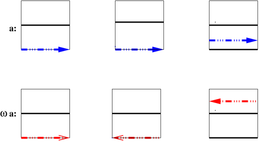
Figure 2: Two distinct brane configurations (denoted by dash-dotted lines): configuration $a$ and its $\omega$ image in the case of D6-branes being split away from the orientifold plane in one, say, third, two-torus. Bold solid lines denote the orientifold planes.

When one moves branes away from the O6-plane in only one two-torus direction, $e.g.$, the third one, there are two distinct configurations: $a$ and $\omega a$ (see Figure 2). However, these configurations are invariant under the two remaining Chan-Paton projections, $i.e.$, $\gamma_{\Omega R\omega}$ and $\gamma_{\theta}$, which yield the symmetry breaking pattern with $Sp$ gauge groups. Specifically, if one takes $2(2k_{i})$-multiples of D6-branes, the symmetry breaking chain is:

$$Sp(2N) \to \hbox{(due to branes on two images)}\,Sp(2N-2k_{i})\times U(2k_{i})\,$$ (9)

$$\to \hbox{(due to}\ \gamma_{\Omega R\omega}\hbox{ and }\gamma_{\theta}\,)\ Sp(2N-2k_{i})\times Sp(2k_{i})~{}.~{}\,$$

More explicitly, the Chan-Paton factor $\lambda$ for the gauge bosons associated with the $2(2k_{i})$ D6-branes moved in one two-torus direction is subject to the following projections:

$$\lambda = -\gamma_{\Omega R}\,\gamma_{\omega}\,\lambda^{T}\,\gamma_{\omega}^{-1}\,\gamma_{\Omega R}^{-1},$$

$$\lambda = \gamma_{\theta}\,\lambda\,\gamma_{\theta}^{-1},$$ (10)

and therefore the final form of $\lambda$ is:

$$\lambda = \pmatrix{A_{1}&0&0&B_{1}\cr 0&A_{2}&B_{2}&0\cr 0&C_{2}&-A_{2}^{T}&0\cr C_{1}&0&0&-A_{1}^{T}\cr}\,,$$ (11)

where $A_{1}$ and $A_{2}$ are arbitrary $k_{i}\times k_{i}$ matrices, and $B_{1}$, $B_{2}$, $C_{1}$ and $C_{2}$ are $k_{i}\times k_{i}$ symmetric matrices. This is precisely the Chan-Paton matrix, which can be cast after a suitable interchange of rows and columns in a block-diagonal form. This structure is associated with the gauge symmetry of configuration $a$, say, the matrices with subscript 1, for the adjoint representation of $Sp(2k_{i})$, and the $\omega\,a$ image, say, the matrices with subscript 2, also for the adjoint representation of $Sp(2k_{i})$. The action of $\gamma_{\omega}$ on the above Chan-Paton matrix precisely interchanges matrices with index 1 and 2: $A_{1}\to A_{2}$, $B_{1}\to-B_{2}$ and $C_{1}\to-C_{2}$, and then effectively maps the Chan-Paton indices of configuration $a$ to those of the image $\omega\,a$. (see Figure 2). Thus, the resulting gauge group is $Sp(2k_{i})$.

The above result is unique. Even though we started with the general $\lambda$, the $\gamma_{\theta}$ and $\gamma_{\Omega\,R\,\omega}$ produced the form in Eq. (11) that can be cast in a block-diagonal form associated with the gauge structure of the $a$ and $\omega\,a$ configurations. The result is the same with the more restricted Ansatz:

$$\lambda = \pmatrix{A_{1}&0&0&B_{1}\cr 0&A_{2}&B_{2}&0\cr 0&C_{2}&D_{2}&0\cr C_{1}&0&0&D_{1}\cr}\,,$$ (12)

where $A_{1,2},\ B_{1,2},\ C_{1,2},\ D_{1,2}$ are general $N\times N$ matrices. This is compatible with the action of $\gamma_{\omega}$, i.e., it interchanges the matrices with index 1 and 2 associated with $a$ and $\omega a$ configurations, respectively. Before the $\gamma_{\theta}$ and $\gamma_{\Omega R\omega}$ projections the gauge group is $U(2k_{i})$, associated with $2k_{i}$ branes for each of the two configurations.

D-Branes splitting in two two-tori

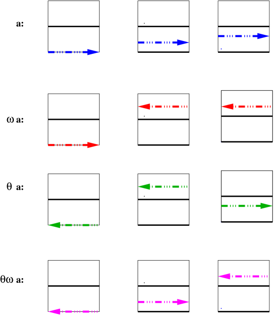
Figure 3: Four distinct brane configurations: $a$ and its $\omega$ , $\theta$ and $\theta\,\omega$ images in the case of D6-branes being split away from the orientifold plane in two two-tori directions, say, in the second and third two-torus.

When one moves branes away from the O6-plane in two two-tori directions, there are four distinct configurations: $a$, $\theta a$, $\omega a$ and $\theta\omega a$ (see Figure 3). The Chan-Paton matrix that reflects the orbifold action on these four configurations can be cast in the form:

$$\lambda = \pmatrix{0&A_{1}&0&0&0&0&B_{1}&0\cr A_{2}&0&0&0&0&0&0&B_{2}\cr 0&0&0&A_{3}&B_{3}&0&0&0\cr 0&0&A_{4}&0&0&B_{4}&0&0\cr 0&0&C_{4}&0&0&D_{4}&0&0\cr 0&0&0&C_{3}&D_{3}&0&0&0\cr C_{2}&0&0&0&0&0&0&D_{2}\cr 0&C_{1}&0&0&0&0&D_{1}&0\cr}\,,$$ (13)

or

$$\lambda = \pmatrix{A_{1}&0&0&0&0&0&B_{1}&0\cr 0&A_{2}&0&0&0&0&0&B_{2}\cr 0&0&A_{3}&0&B_{3}&0&0&0\cr 0&0&0&A_{4}&0&B_{4}&0&0\cr 0&0&C_{3}&0&D_{3}&0&0&0\cr 0&0&0&C_{4}&0&D_{4}&0&0\cr C_{1}&0&0&0&0&0&D_{1}&0\cr 0&C_{2}&0&0&0&0&0&D_{2}\cr}\,,$$ (14)

where $A_{1,2,3,4}$, $B_{1,2,3,4}$, $C_{1,2,3,4}$, and $D_{1,2,3,4}$ are general $k_{i}\times k_{i}$ matrices. The gauge group is $U(2k_{i})$ associated with $(2k_{i})$ branes on each of the four configurations. The $8\times 8$ matrix $\lambda$, whose entries are $k_{i}\times k_{i}$ matrices, can be considered as a $4\times 4$ matrix, where all the entries are $2\times 2$ matrices in which each entry is still a $k_{i}\times k_{i}$ matrix. These $2\times 2$ matrices like in Eq. (14) must be diagonal because the off-diagonal components correspond to the open string states which stretch between the different stacks (images) of D6-branes and then are massive. However, there is still one remaining nontrivial projection on Chan-Paton indices, say, $\gamma_{\Omega R\omega}$ under which these configurations are invariant if branes are moved away in the second and third two-tori directions (see Figure 3). In this case the $\gamma_{\Omega R\omega}$ projection (with representation in Eq. (3)) acts separately on the matrices with indices $1$, $2$, $3$ and $4$, yielding:

$$\lambda = \pmatrix{0&A_{1}&0&0&0&0&B_{1}&0\cr A_{2}&0&0&0&0&0&0&B_{2}\cr 0&0&0&A_{3}&B_{3}&0&0&0\cr 0&0&A_{4}&0&0&B_{4}&0&0\cr 0&0&C_{4}&0&0&-A_{4}^{T}&0&0\cr 0&0&0&C_{3}&-A_{3}^{T}&0&0&0\cr C_{2}&0&0&0&0&0&0&-A_{2}^{T}\cr 0&C_{1}&0&0&0&0&-A_{1}^{T}&0\cr}\,,$$ (15)

or

$$\lambda = \pmatrix{A_{1}&0&0&0&0&0&B_{1}&0\cr 0&A_{2}&0&0&0&0&0&B_{2}\cr 0&0&A_{3}&0&B_{3}&0&0&0\cr 0&0&0&A_{4}&0&B_{4}&0&0\cr 0&0&C_{3}&0&-A_{3}^{T}&0&0&0\cr 0&0&0&C_{4}&0&-A_{4}^{T}&0&0\cr C_{1}&0&0&0&0&0&-A_{1}^{T}&0\cr 0&C_{2}&0&0&0&0&0&-A_{2}^{T}\cr}\,,$$ (16)

where $A_{1,2,3,4}$ are general $k_{i}\times k_{i}$ matrices, and $C_{1,2,3,4}$ and $B_{1,2,3,4}$ are symmetric $k_{i}\times k_{i}$ matrices. Therefore, the gauge symmetry is $Sp(2k_{i})$ with the Chan-Paton matrix associated with all four configurations $a$, $\omega a$, $\theta a$ and $\theta\omega a$.

In this process, one takes $2(4k_{i})$-multiples of branes and the breaking pattern is:

$$Sp(2N) \to \hbox{(due to branes on four images)}\ Sp(2N-4k_{i})\times U(2k_{i})$$ (17)

$$\to \hbox{(due to}\ \gamma_{\Omega R\omega})\ Sp(2N-4k_{i})\times Sp(2k_{i})~{}.~{}\,$$

D-Branes splitting in three two-tori

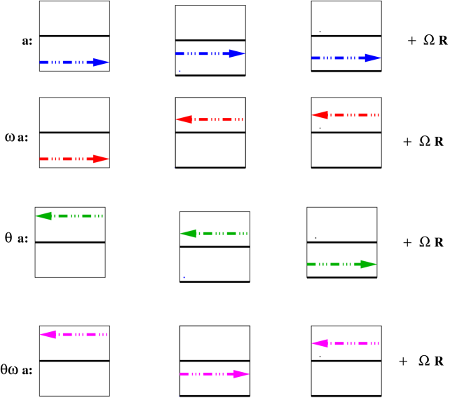
Figure 4: Four distinct brane configurations: $a$ configuration, its $\omega$ , $\theta$ and $\theta\omega$ images as well as four $\Omega\,R$ (not depicted on the figure) in the case of D6-branes being split away from the orientifold plane in all three two-tori directions.

If one splits D6-branes in all three toroidal directions, there are now eight distinct configurations: $a$, $\theta\,a$, $\omega\,a$, ${\omega\,\theta\,a}$, and four new images due to the $\Omega\,R$ action (see Figure 4). Thus one has to move away from the O6-planes at least eight multiples of branes. Since there is no further projection on Chan-Paton indices, moving sets of $2(4k_{i})$ branes away from O6-planes in all three toroidal directions results in the symmetry breaking pattern:

$$Sp(2N)\to\hbox{(due to branes on eight images)}\ Sp(2N-4k_{i})\times U(k_{i})~{}.~{}\,$$ (18)

In general, if we split $2(2k_{i}^{1})$ D6-branes in any one of the three two-tori, $2(4k_{j}^{2})$ D6-branes in any two of the three two-tori, and $2(4k_{l}^{3})$ D6-branes in three two-tori, the gauge symmetry breaking pattern is:

$$Sp(2N) \to Sp(2N-\sum_{i}2k^{1}_{i}-\sum_{j}4k^{2}_{j}-\sum_{l}4k_{l}^{3})\times\prod_{i}Sp(2k^{1}_{i})$$ (19)

$$\times\prod_{j}Sp(2k^{2}_{j})\times\prod_{l}U(k_{l}^{3})~{}.~{}\,$$

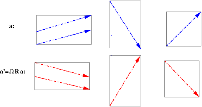
Figure 5: The D6-brane configuration (dash-dotted line) wrapping a (supersymmetric) three-cycle invariant under orbifold projection. The second configuration is its orientifold image.

2.2 D6-Branes not Parallel to O6-Planes

For completeness let us also mention the splitting of D6-branes in stacks that are not parallel to the O6-planes. In particular, one chooses first $2(2N)$ D6-branes, wrapping a factorizable three-cycle that is invariant under the $\bf Z_{2}\times\bf Z_{2}$ action. In this case $2N$ D6-branes wrap the original three-cycle, i.e., configuration $a$, and $2N$ branes wrap a three-cycle that is its $\Omega\,R$ image, i.e., the configuration $a^{\prime}\equiv\Omega\,R\,a$ (see Figure 5). The Chan-Paton matrix can therefore be cast in a block diagonal from:

$$\lambda={\rm diag\,}(A\,;D)\,,$$ (20)

where $A$ and $D$ are general $2N\times 2N$ matrices, associated with the $a$ and $a^{\prime}$ configurations, respectively. Since the $\gamma_{\theta}$ and $\gamma_{\omega}$ matrices in Eq. (3) are also diagonal, it is sufficient to do projections only on the $A$ matrix. (The action on $D$ goes in parallel and just reflects the fact that for each $a$ there is an $a^{\prime}$ image.) Since the $a$ configuration is invariant under $\theta$ and $\omega$ actions, one has to perform the $\gamma_{\theta}$ and $\gamma_{\omega}$ projections on the Chan-Paton indices, yielding the $U(N)$ group factor [7].

D-Branes splitting in one two-torus

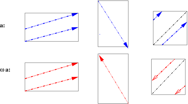
Figure 6: The D6-brane configuration (dash-dotted line) wrapping a (supersymmetric) 3-cycle which is not invariant under the orbifold projection, say in the third two-torus. Its $\omega$ image is therefore a different configuration.

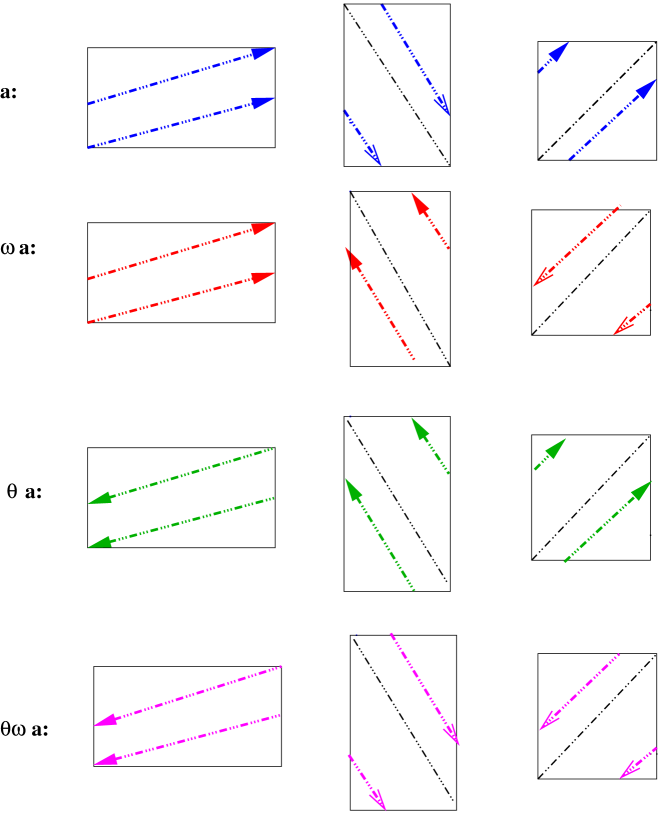
Figure 7: The D6-brane configuration (dash-dotted line) wrapping a (supersymmetric) 3-cycle which is not invariant under the orbifold projection, say in the second and third two-tori. Its three orbifold images are therefore different configurations.

When one moves $2(2k_{i})$ branes in one two-torus direction, e.g., in the third two-torus direction, there is now the $a$-configuration and its $\omega\ a$ image (in addition to the $a^{\prime}$-configuration and $\omega\ a^{\prime}$ image), see Figure 6. It is sufficient to perform the $\theta$ projection on the Chan-Paton matrix $\lambda$, which is a $2k_{i}\times 2k_{i}$ matrix of the form:

$$\lambda = \pmatrix{A_{1}&0\cr 0&A_{2}\cr}\,,$$ (21)

where $A_{1}$ and $A_{2}$ are arbitrary $k_{i}\times k_{i}$ matrices. This restricted form of the matrix is compatible with the action of $\gamma_{\omega}$: $A_{1}\to A_{2}$, mapping the Chan-Paton indices of the $a$ configuration to those of $\omega\,a$. (Actions on orientifold images $D_{1}$ and $D_{2}$ of course go in paprallel.) So, the gauge group is $U(k_{i})$.

The representation of $\gamma_{\theta}$ is only the upper half of the matrix $\gamma_{\theta}$ in Eq. (3) because we neglect the $\Omega\,R$ images. Then the matrix in Eq. (21) is invariant under $\gamma_{\theta}$ projection. Therefore, the gauge symmetry in this case is still $U(k_{i})$ and the breaking pattern is of the form:

$$U(N) \to \hbox{(due to branes on two images)}\,U(N-k_{i})\times U(k_{i})\,$$ (22)

$$\to (\hbox{due to}\ \gamma_{\theta}\ )\ U(N-k_{i})\,\times U(k_{i})\,.$$

D-Branes splitting in two two-tori

When one moves branes in two two-tori directions, there are four distinct configurations: $a$, $\theta\,a$, $\omega\,a$ and $\theta\,\omega\,a$ (and of course four distinct $\Omega R$ images), see Figure 7. In this case, one has to take $2(4k_{i})$ branes and put them on all these distinct configurations (there are no projections on Chan-Paton indices). The symmetry breaking pattern is:

$$U(N)\to\hbox{(due to branes on four images)}\,U(N-2k_{i})\times U(k_{i})\,.$$ (23)

D-Branes splitting in three two-tori

When one moves branes in all three two-torus directions, there are no new images and thus the symmetry breaking pattern is the same as that in Eq. (23). In spite of having the same symmetry breaking pattern, the geometric interpretation of this configuration is of course different from that of the D-brane splitting in two two-tori since now the splitting takes place in all three toroidal directions. On the dual field theory side, we shall see that in this case the deformation in all three toroidal directions corresponds to giving VEV’s to three superfields-moduli in the adjoint representation.

In general, if we split $2(2k_{i}^{1})$ D6-branes in any one of the three two-tori, $2(4k_{j}^{2})$ D6-branes in any two of the three two-tori, and $2(4k_{l}^{3})$ D6-branes in three two-tori, the gauge symmetry breaking pattern is:

$$U(N) \to U(N-\sum_{i}k^{1}_{i}-\sum_{j}2k^{2}_{j}-\sum_{l}2k_{l}^{3})\times\prod_{i}U(k^{1}_{i})$$ (24)

$$\times\prod_{j}U(k^{2}_{j})\times\prod_{l}U(k_{l}^{3})~{}.~{}\,$$

In sum, in the three cases discussed the field theory corresponds to giving VEVs to one, two and three chiral superfields in the anti-symmetric representation of $Sp(2N)$ or adjoint representation of $U(N)$, respectively. A detailed discussion of this field theoretical interpretation via Higgsing will be given in the next Section.

3 Higgsings in Field Theory

3.1 Higgsings for D-Branes Parallel to the O6-Planes

The D6-brane geometric operations discussed in the previous Section are in one-to-one correspondence with the field theory Higgs mechanism, by giving VEVs to three chiral superfields-moduli living on D6-branes. [These three adjoint (or anti-symmetric) chiral super-multiplets for the $U(N)$ (or $Sp(2N)$) group are generated from the decomposition of the original adjoint vector representation of D9-branes, which is caused by the dimensional reduction of D9-branes down to D6-branes due to T-duality in three directions.] For definiteness, we shall focus on the relatively complicated gauge symmetry breaking pattern

$$Sp(4k) \rightarrow Sp(2k)\times Sp(2k)$$ (25)

$$\rightarrow Sp(2k)$$

$$\rightarrow U(k)~{},~{}\,$$

given by Eq. (18). This pattern happens when one moves D6-branes off the O6-planes in all two-tori directions, which requires all three anti-symmetric chiral supermultiplets to obtain VEVs, each one being responsible for one breaking step. The analysis will be very similar for the other gauge symmetry breaking patterns in Eqs. (9) and (17) where one splits the D6-branes off the O6-planes in one and two two-tori, respectively.

To start with, let us review some simple properties of $Sp$ groups. $Sp(2N)$ is defined as the group of pseudo orthogonal transformations preserving the anti-symmetric inner product

$$\eta_{\alpha}\Sigma_{\alpha\beta}\xi_{\beta}~{},~{}$$ (26)

where $\Sigma=\sigma_{2}\bigotimes I_{N\times N}$. The generators must satisfy the algebraic condition

$$T^{T}\Sigma+\Sigma T=0~{}.~{}$$ (27)

Their representations then can be expanded in the direct product form

$$T = I_{2\times 2}\bigotimes T_{a}+\vec{\sigma}\bigotimes\vec{T_{s}}$$ (28)

$$=\left(\matrix{{A_{N}}&{S_{N}^{1}}\cr{S_{N}^{2}}&{-A_{N}^{T}}}\right)~{},~{}$$

where $A_{N}=T_{a}+T_{s}^{3}$, $S_{N}^{1}=T_{s}^{1}-T_{s}^{2}$ and $S_{N}^{2}=T_{s}^{1}+T_{s}^{2}$ are $N\times N$ matrices with $T_{a}=-T_{a}^{T}$ and $T_{s}=T_{s}^{T}$. For the special case $T_{S}^{1}=T_{S}^{2}=0$, the representations are reduced to

$$T=\left(\matrix{{A_{N}}&{0}\cr{0}&{-A_{N}^{T}}}\right)~{},~{}$$ (29)

leaving the $Sp(2N)$ subgroup $U(N)$. For convenience we have taken a real convention for the Pauli matrices,

$$\sigma_{1}=\left(\matrix{{0}&{1}\cr{1}&{0}}\right), \sigma_{2}=\left(\matrix{{0}&{-1}\cr{1}&{0}}\right), \sigma_{3}=\left(\matrix{{1}&{0}\cr{0}&{-1}}\right).$$ (30)

It is convenient to employ a tensor language in which the indices are raised by $\Sigma^{T}$ and lowered by $\Sigma$. The invariant pseudo inner product then can be rewritten as

$$\eta^{\alpha}\xi_{\alpha}~{},~{}$$ (31)

which obeys the transformation laws

$$\xi_{\alpha}\rightarrow\xi_{\alpha}+(T\xi)_{\alpha}~{},~{}$$ (32)

$$\eta^{\alpha}\rightarrow\eta^{\alpha}-(\eta T)^{\alpha}~{}.~{}\,$$ (33)

There are three $N=1$ anti-symmetric chiral supermultiplets for the $Sp$ gauge factor on filler branes. Raising one index of these representations, they will obey the transformation law

$$\Phi_{\alpha}^{\beta}\rightarrow\Phi_{\alpha}^{\beta}+(T\Phi)_{\alpha}^{\beta}-(\Phi T)_{\alpha}^{\beta}~{},~{}$$ (34)

and can be expanded as

$$\Phi_{\alpha}^{\beta}=I\bigotimes\Phi_{s}+\vec{\sigma}\bigotimes\vec{\Phi}_{a}~{},~{}$$ (35)

where $\Phi_{s}^{T}=\Phi_{s}$ and $\vec{\Phi}_{a}^{T}=-\vec{\Phi}_{a}$. $\Phi_{\alpha}^{\beta}$ and the $Sp$ generators $T$ have different expansion forms since they belong to different representations. By giving $\Phi^{a}$, $\Phi^{b}$ and $\Phi^{c}$ VEVs

$$\langle\Phi^{a}\rangle=I\bigotimes v^{a}\left(\matrix{{I_{k}}&{0}\cr{0}&{-I_{k}}}\right)~{},~{}$$ (36)

$$\langle\Phi^{b}\rangle=I\bigotimes v^{b}\left(\matrix{{0}&{I_{k}}\cr{I_{k}}&{0}}\right)~{},~{}$$ (37)

$$\langle\Phi^{c}\rangle=\sigma_{3}\bigotimes v^{c}\left(\matrix{{0}&{I_{k}}\cr{-I_{k}}&{0}}\right)~{},~{}$$ (38)

the original $Sp(4k)$ symmetry will be broken down to $U(k)$ step by step. If we diagonalize the matrices $\langle\Phi^{a}\rangle$, $\langle\Phi^{b}\rangle$ and $\langle\Phi^{c}\rangle$, we obtain two eigenvalues with the same magnitude but opposite sign for each one, which indicates that the D6-branes are split on each two-torus.

To discuss the gauge symmetry breaking, let us explicitly write the direct product expansions for the $Sp(4k)$ adjoint representation

$$T=I\bigotimes\left(\matrix{{(T_{a})_{11}}&{(T_{a})_{12}}\cr{-(T_{a})_{12}^{T}}&{(T_{a})_{22}}}\right)+\vec{\sigma}\bigotimes\left(\matrix{{(\vec{T_{s}})_{11}}&{(\vec{T_{s}})_{12}}\cr{(\vec{T_{s}})_{12}^{T}}&{(\vec{T_{s}})_{22}}}\right)~{},~{}$$ (39)

where the diagonal entries of $T_{a}$ and $T_{s}$ are $k\times k$ matrices which satisfy $(T_{a})_{ii}=-(T_{a})_{ii}^{T}$, $(\vec{T_{s}})_{ii}=(\vec{T_{s}})_{ii}^{T}$ and the off-diagonal entries $(T_{a})_{12}$, $(\vec{T_{s}})_{12}$ are arbitrary. Once $\Phi^{a}$, $\Phi^{b}$ or $\Phi^{c}$ obtains VEVs, only those symmetries commuting with $\langle\Phi^{a}\rangle$, $\langle\Phi^{b}\rangle$ or $\langle\Phi^{c}\rangle$ survive. Given

$$(X_{1}\bigotimes Y_{1})(X_{2}\bigotimes Y_{2})=(X_{1}X_{2})\bigotimes(Y_{1}Y_{2})$$ (40)

$$Tr(X\bigotimes Y)=(TrX)(TrY)~{},~{}$$ (41)

one obtains

$$[T,\langle\Phi^{a}\rangle] = I\bigotimes 2v^{a}\left(\matrix{{0}&{-(T_{a})_{12}}\cr{-(T_{a})_{12}^{T}}&{0}}\right)$$ (42)

$$+\vec{\sigma}\bigotimes 2v^{a}\left(\matrix{{0}&{-(\vec{T_{s}})_{12}}\cr{-(\vec{T_{s}})_{12}^{T}}&{0}}\right)~{},~{}$$

for a given $T$. The surviving symmetries satisfy

$$(T_{a})_{12}=(\vec{T_{s}})_{12}=0~{},~{}$$ (43)

yielding $Sp(2k)\times Sp(2k)$.

Subsequently, a non-zero $\langle\Phi^{b}\rangle$ leads to

$$[T,\langle\Phi^{b}\rangle] = I\bigotimes v^{b}\left(\matrix{{0}&{(T_{a})_{11}-(T_{a})_{22}}\cr{(T_{a})_{22}-(T_{a})_{11}}&{0}}\right)$$ (44)

$$+\vec{\sigma}\bigotimes v^{b}\left(\matrix{{0}&{(\vec{T_{s}})_{11}-(\vec{T_{s}})_{22}}\cr{(\vec{T_{s}})_{22}-(\vec{T_{s}})_{11}}&{0}}\right)~{}.~{}\,$$

The commutator is invariant if and only if

$$(T_{a})_{11}=(T_{a})_{22}, (\vec{T_{s}})_{11}=(\vec{T_{s}})_{22}~{},~{}$$ (45)

which identifies the two surviving gauge symmetries, leaving $Sp(2k)$.

Finally, if $\Phi^{c}$ also obtains a VEV, the new commutator with the $Sp(2k)$ generators will be

$$[T,\langle\Phi^{c}\rangle] = v^{c}[\vec{\sigma},\sigma_{3}]\bigotimes\left(\matrix{{0}&{(\vec{T_{s}})_{11}}\cr{-(\vec{T_{s}})_{11}}&{0}}\right)~{}.~{}\,$$ (46)

It vanishes if and only if

$$(T_{s}^{1})_{11}=(T_{s}^{2})_{11}=0~{},~{}\,$$ (47)

leaving the surviving symmetries

$$T=I\bigotimes\left(\matrix{{(T_{a})_{11}}&{0}\cr{0}&{(T_{a})_{11}}}\right)+\sigma_{3}\bigotimes\left(\matrix{(T_{s}^{3})_{11}&{0}\cr{0}&{(T_{s}^{3})_{11}}}\right)~{}.~{}\,$$ (48)

Referring to Eq. (29), we see that this is the $U(k)$ group.

Next, let us check D- and F-flatness for these breaking patterns. D-flatness can be directly seen from

$$Tr[\langle\Phi^{i}\rangle^{{\dagger}}T\langle\Phi^{i}\rangle]=0~{},~{}$$ (49)

where $i$ runs over $a$, $b$ and $c$. F-flatness is easy to check, too. The superpotential for $\Phi^{i}$’s is

$$W={\rm Tr}(\Phi^{a}\Phi^{b}\Phi^{c}+\Phi^{a}\Phi^{c}\Phi^{b})$$ (50)

instead of the $N=4$ commutator structure. From Eq. (35) one has

$${\rm Tr}(\Phi^{a}\Phi^{b}\Phi^{c})={\rm Tr}(\Phi^{a}\Phi^{c}\Phi^{b})~{}.~{}\,$$ (51)

For example,

$${\rm Tr}[\Phi^{a}\langle\Phi^{b}\rangle\langle\Phi^{c}\rangle]=2v^{b}v^{c}{\rm Tr}[\Phi_{a}^{3}\left(\matrix{{-I_{k}}&{0}\cr{0}&{I_{k}}}\right)]=0~{},~{}$$ (52)

where $\Phi_{a}^{3}$ is the third anti-symmetric component matrix of $\vec{\Phi}^{a}$. Similarly, ${\rm Tr}[\langle\Phi^{a}\rangle\Phi^{b}\langle\Phi^{c}\rangle]={\rm Tr}[\langle\Phi^{a}\rangle\langle\Phi^{b}\rangle\Phi^{c}]={\rm Tr}[\langle\Phi^{a}\rangle\langle\Phi^{b}\rangle\langle\Phi^{c}\rangle]=0$, so F-flatness is also preserved.

This result is consistent with the symmetry breaking pattern due to the brane splitting in the string theory constructions. The F- and D-flatness preserving VEVs for one, two and three chiral superfields in the anti-symmetric representation of the original $Sp$ group is in one-to-one correspondence with the symmetry breaking pattern due to the splitting of D6-branes, parallel with the O6-planes in one-, two- and three- two-torus directions, respectively. In other words, the three chiral superfields are the moduli associated with the parallel motion of D6-branes wrapping (non-rigid) cycles, parallel with the O6-planes. Note that the D- and F-flatness are not automatically guaranteed for Higgsing if two or three chiral superfields in the anti-symmetric representation of $Sp$ branes (or adjoint representation for $U$ branes) obtain VEVs. However, the D- or F-flatness violating Higgsing does not typically correspond to a consistent deformation of D6-brane configurations.

3.2 Higgsings for D-Branes Not Parallel to the O6-Planes

For the sake of completeness, in this subsection we shall also discuss the Higgsing for the D6-branes not parallel to the O6-planes. The string theory aspects of symmetry breaking via such D6-brane splitting have been discussed in Section 2.2. Here we give the dual field theory description of the symmetry breaking via the supersymmetry preserving Higgs mechanism due to the three chiral superfields in the adjoint representation of $U(N)$.

Recall, the $U(N)$ symmetry breaking chain due to brane-splitting is:

$$U(N) \rightarrow U(N-k)\times U(k)$$ (53)

$$\rightarrow U(N-2k)\times U(k)$$

$$\rightarrow U(N-2k)\times U(k)~{}.~{}\,$$

In the canonical generator basis for the $U(N)$ group, we choose the VEVs of $\Phi^{a}$, $\Phi^{b}$ and $\Phi^{c}$ as

$$\langle\Phi^{a}\rangle~{}=~{}\left(\matrix{-v_{a}I_{k\times k}&0_{k\times(N-k)}\cr 0_{(N-k)\times k}&v_{a}I_{(N-k)\times(N-k)}}\right)~{},~{}\,$$ (54)

$$\langle\Phi^{b}\rangle=\left(\matrix{0_{k\times k}&v_{b}I_{k\times k}&0_{k\times(N-2k)}\cr v_{b}I_{k\times k}&0_{k\times k}&0_{k\times(N-2k)}\cr 0_{(N-2k)\times k}&0_{(N-2k)\times k}&0_{(N-2k)\times(N-2k)}}\right)~{},~{}\,$$ (55)

$$\langle\Phi^{c}\rangle=\left(\matrix{0_{k\times k}&-iv_{c}I_{k\times k}&0_{k\times(N-2k)}\cr iv_{c}I_{k\times k}&0_{k\times k}&0_{k\times(N-2k)}\cr 0_{(N-2k)\times k}&0_{(N-2k)\times k}&0_{(N-2k)\times(N-2k)}}\right)~{},~{}\,$$ (56)

where $I_{n\times n}$ is the $n\times n$ identity matrix, and $0_{n\times m}$ is the $n\times m$ matrix in which all the entries are zero.

It can easily be shown that $\Phi^{a}$ breaks the $U(N)$ gauge symmetry down to $U(N-k)\times U(k)$, and $\Phi^{b}$ breaks $U(N-k)\times U(k)$ to $U(N-2k)\times U(k)$. However, $\Phi^{c}$ does not lead to a further breaking of the gauge symmetry, similar to the gauge symmetry breaking via brane splitting.

D-flatness can be obtained from

$$D^{a}\equiv{\rm Tr}\left(\langle\Phi^{i}\rangle^{{\dagger}}[T^{a},\langle\Phi^{i}\rangle]\right)=0~{},~{}$$ (57)

where $i$ runs over $a$, $b$ and $c$, and $T^{a}$ is the generator of $U(N)$.

The superpotential for $\Phi^{i}$’s can be written as (see e.g., [7]):

$$W={\rm Tr}\left(\Phi^{a}\Phi^{b}\Phi^{c}+\Phi^{b}\Phi^{a}\Phi^{c}\right)~{}.~{}\,$$ (58)

The superpotential can easily be seen to vanish when any two (or all three) of $\Phi^{a}$, $\Phi^{b}$ and $\Phi^{c}$ obtain VEVs, demonstrating F-flatness.

4 Standard-like Models and Brane-Splitting

One natural way to obtain the three-family $N=1$ supersymmetric standard-like models via D6-brane-splitting was addressed in [26]. One started with the Pati-Salam gauge symmetry $U(4)\times U(2)_{L}\times U(2)_{R}$ in the observable sector. The left-right symmetric model $SU(3)\times SU(2)_{L}\times SU(2)_{R}\times U(1)_{B-L}$ was then obtained by splitting $U(4)$ branes, and the gauge symmetry $SU(3)_{C}\times SU(2)_{L}\times U(1)_{B-L}\times U(1)_{R}$ was obtained by further splitting $U(2)_{R}$ branes. Finally, the Standard Model gauge symmetry emerged by giving VEV’s to the massless open string states in an $N=2$ subsector, i.e., the field theory analog of brane recombination.

In this Section, we shall further explore the construction of the Standard-like models, by employing the D6-brane splitting mechanism for the $\bf Z_{2}\times\bf Z_{2}$ orientifold models. Here, the electroweak symmetry will emerge primarily from the splitting of D6-branes parallel with the O6-planes. Within the supersymmetric constructions with intersecting D6-branes, this possibility has not been explored, yet. Such Standard-like models shall be generated for two Pati-Salam-like models. For the first example we shall employ the D-brane splitting as discussed in Sections 3 and 4; this procedure of course preserves supersymmetry and corresponds to the consistent string construction. For the second model we will present the Higgs mechanism that breaks it down to the three family Standard Model, but unfortunately it does not preserve the D- and F-flatness condition. This Higgsing procedure therefore does not have an interpretation in terms of a consistent D-brane splitting construction. The main difference in comparison with the models discussed in [26] is that now the starting electroweak symmetry is based on $Sp$ groups, i.e., $U(4)\times Sp(8\ {\rm or}\ 6)_{L}\times Sp(8\ {\rm or}\ 6)_{R}$, and not on $U$ groups, i.e., $U(4)\times U(2)_{L}\times U(2)_{R}$, as in [26]. We shall allow for the brane splitting for all three brane stacks, leading to $SU(3)\times Sp(2)_{L}\times Sp(2)_{R}\times U(1)_{B-L}$, again. In particular, for the four-family supersymmetric model, its observable sector and the hidden sector do not spatially intersect, therefore yielding no massless exotic particles.

The third model presented in Section 4.3 is the three-family Standard-like model based directly on the $Sp(2)_{L}\times Sp(2)_{R}$ brane constrcution. It is related to the local construction in [36, 37]. Our construction is a consistent supersymmetric one, but it suffers from the Standard Model chiral exotics.

4.1 Model I: Four Family Standard-like Model

Table 2: D6-brane configurations and intersection numbers for the four-family Standard-like model. In the table, $\chi_{i}$ is the complex modulus for the $i-$th torus, and $\beta_{i}^{g}$ is the beta function for the $i-$th $Sp$ group from the $i-$th stack of branes.

I	$[U(4)_{C}\times Sp(8)_{L}\times Sp(8)_{R}]_{observed}\times[U(4)\times Sp(8)\times Sp(8)]_{hidden}$
stack	$N$	$(n^{1},l^{1})\times(n^{2},l^{2})\times(n^{3},l^{3})$	$n_{\raisebox{-0.5pt}{\hbox{\rule{0.4pt}{6.5pt}\hskip-0.4pt\rule{6.5pt}{0.4pt}\hskip-6.5pt\rule[6.5pt]{6.5pt}{0.4pt}}\rule[6.5pt]{0.4pt}{0.4pt}\hskip-0.4pt\rule{0.4pt}{6.5pt}}\hskip-0.4pt\raisebox{-0.5pt}{\hbox{\rule{0.4pt}{6.5pt}\hskip-0.4pt\rule{6.5pt}{0.4pt}\hskip-6.5pt\rule[6.5pt]{6.5pt}{0.4pt}}\rule[6.5pt]{0.4pt}{0.4pt}\hskip-0.4pt\rule{0.4pt}{6.5pt}}}$	$n_{\raisebox{-3.5pt}{\hbox{\rule{0.4pt}{6.5pt}\hskip-0.4pt\rule{6.5pt}{0.4pt}\hskip-6.5pt\rule[6.5pt]{6.5pt}{0.4pt}}\rule[6.5pt]{0.4pt}{0.4pt}\hskip-0.4pt\rule{0.4pt}{6.5pt}}\hskip-6.9pt\raisebox{3.0pt}{\hbox{\rule{0.4pt}{6.5pt}\hskip-0.4pt\rule{6.5pt}{0.4pt}\hskip-6.5pt\rule[6.5pt]{6.5pt}{0.4pt}}\rule[6.5pt]{0.4pt}{0.4pt}\hskip-0.4pt\rule{0.4pt}{6.5pt}}}$	$b$	$c$	$d$	$d^{\prime}$	1	2
$a$	8	$(1,0)\times(1,1)\times(1,-1)$	0	0	1	-1	0	0	0	0
$b$	8	$(0,1)\times(1,0)\times(0,-1)$	0	0	-	0	0	0	0	0
$c$	8	$(0,1)\times(0,-1)\times(1,0)$	0	0	-	-	0	0	0	0
$d$	8	$(0,1)\times(1,-1)\times(1,-1)$	0	0	-	-	-	0	-1	1
1	8	$(1,0)\times(1,0)\times(1,0)$	$\chi_{2}=\chi_{3}=1$
2	8	$(1,0)\times(0,-1)\times(0,1)$	$\beta^{g}_{1}=\beta^{g}_{2}=-4$

Model I is a four-family model, with its D6-brane configurations and intersection numbers listed in Table 2. This model contains $U(4)_{C}\times Sp(8)_{L}\times Sp(8)_{R}$ and $U(4)\times Sp(8)\times Sp(8)$ gauge structures in its observable and hidden sectors, respectively. [For technical details and consistency conditions for RR-tadpole free supersymmetric constructions see [7, 22, 26].] From the wrapping numbers of the stacks of D6-branes, it is not hard to check that no intersection happens between these two sectors and thus the chiral Standard Model exotic particles, which had been a generic problem for supersymmetric constructions with intersecting D6-branes, are absent here.

Let us focus on the observable sector first. As discussed in the previous Sections the $Sp(4k)$ group can be broken down to $U(k)$ symmetry by moving D6-branes off O6-planes in all two-tori directions. This indicates that the $Sp(8)_{L}\times Sp(8)_{R}$ gauge factors in this model can be diagonally broken down to $U(2)_{L}\times U(2)_{R}$.

In this case both $U(1)$ factors are non-anomalous since they arise from the non-Abelian, i.e., $Sp$, symmetry. (All non-Abelian gauge symmetries in these string constructions are non-anomalous [7].) Meanwhile, the original chiral supermultiplets , $i.e.$, $(4,8,1;1,1,1)$ and $(4,1,8;1,1,1)$ are decomposed into four identical ones, $i.e.$, $(4,2,1;1,1,1)$ and $(4,1,2;1,1,1)$, respectively. Note that the four families in the effective theory have been obtained from a single family in the original construction. The fact that the number of families can change for this type of Higgsing has the string origin in the original configuration on the top of the O6-plane, i.e., the singular configuration, fixed by the orientifold action. The subsequent splitting of branes away from this singularity in turn allows for the change in the number of chiral families. Furthermore, this specific Higgsing, as discussed in the previous Section, preserves D- and F-flatness and thus the breaking can take place at the string scale. Namely, in the dual string theory, the brane-splitting can take place at any separation of branes, limited only by the size of the internal space.

After the brane-splitting, as discussed above, the resulting “observable sector” is therefore a four-family Pati-Salam model $U(4)\times U(2)_{L}\times U(2)_{R}$. As for the “hidden sector”, all the $Sp$ gauge factors have negative $\beta$ functions and therefore allow for confinement at some intermediate scale and gaugino condensation there. This mechanism would in turn generate a non-perturbative effective superpotential compactification moduli, which could allow for the ground state solution with stabilized moduli. For more details, see [19].

4.2 Model II: Non-Supersymmetric Three Family Standard Model

Table 3: D6-brane configurations and intersection numbers for the three-family Standard-like model. In the table, $\chi_{i}$ is the complex modulus for the $i-$th torus, and $\beta_{i}^{g}$ is the beta function for the $i-$th $Sp$ group from the $i-$th stack of branes. The third torus is tilted, so $l^{3}=n^{3}+2m^{3}$[22].

II	$[U(4)_{C}\times Sp(6)_{L}\times Sp(6)_{R}]_{observed}\times[U(2)\times Sp(4)\times Sp(4)]_{hidden}$
stack	$N$	$(n^{1},l^{1})\times(n^{2},l^{2})\times(n^{3},l^{3})$	$n_{\raisebox{-0.5pt}{\hbox{\rule{0.4pt}{6.5pt}\hskip-0.4pt\rule{6.5pt}{0.4pt}\hskip-6.5pt\rule[6.5pt]{6.5pt}{0.4pt}}\rule[6.5pt]{0.4pt}{0.4pt}\hskip-0.4pt\rule{0.4pt}{6.5pt}}\hskip-0.4pt\raisebox{-0.5pt}{\hbox{\rule{0.4pt}{6.5pt}\hskip-0.4pt\rule{6.5pt}{0.4pt}\hskip-6.5pt\rule[6.5pt]{6.5pt}{0.4pt}}\rule[6.5pt]{0.4pt}{0.4pt}\hskip-0.4pt\rule{0.4pt}{6.5pt}}}$	$n_{\raisebox{-3.5pt}{\hbox{\rule{0.4pt}{6.5pt}\hskip-0.4pt\rule{6.5pt}{0.4pt}\hskip-6.5pt\rule[6.5pt]{6.5pt}{0.4pt}}\rule[6.5pt]{0.4pt}{0.4pt}\hskip-0.4pt\rule{0.4pt}{6.5pt}}\hskip-6.9pt\raisebox{3.0pt}{\hbox{\rule{0.4pt}{6.5pt}\hskip-0.4pt\rule{6.5pt}{0.4pt}\hskip-6.5pt\rule[6.5pt]{6.5pt}{0.4pt}}\rule[6.5pt]{0.4pt}{0.4pt}\hskip-0.4pt\rule{0.4pt}{6.5pt}}}$	$b$	$c$	$d$	$d^{\prime}$	1	2
$a$	8	$(1,0)\times(1,1)\times(1,-1)$	0	0	1	-1	0	0	0	0
$b$	6	$(0,1)\times(1,0)\times(0,-2)$	0	0	-	0	0	0	0	0
$c$	6	$(0,1)\times(0,-1)\times(2,0)$	0	0	-	-	0	0	0	0
$d$	4	$(0,1)\times(1,-1)\times(1,-1)$	$\chi_{2}=\frac{1}{2}\chi_{3}=1$
1	4	$(1,0)\times(1,0)\times(2,0)$	$\beta^{g}_{1}=-5$, $\beta^{g}_{2}=-5$
2	4	$(1,0)\times(0,-1)\times(0,2)$

Model II is a three-family model, with its D6-brane configurations and intersection numbers given in Table 3. This model contains $U(4)_{C}\times Sp(6)_{L}\times Sp(6)_{R}$ and $U(2)\times Sp(4)\times Sp(4)$ gauge structures in its observable and hidden sectors, respectively. This model also shares the advantage of Model I, $i.e.$, there are no massless Standard Model chiral exotics since the branes in the observable and hidden sectors do not intersect at a point in the internal space. [First version had chiral exotics and suffered from the global anomaly [39], due to the odd number of fundamental representations under $Sp(2N)$ symmetries.]

However, in this model the Higgsing down to the Standard Model symmetry with three-families breaks supersymmetry since such a symmetry breaking pattern does not preserve the F- and D-flatness conditions. Alternatively, there is no pallel D-brane splitting that would result in such a symmmetry breaking pattern. Nevertheless let us consider one typical breaking pattern:

$$Sp(6) \rightarrow Sp(2)\times Sp(2)\times Sp(2)$$ (59)

$$\rightarrow Sp(2)\times Sp(2)$$

$$\rightarrow Sp(2)~{}.~{}\,$$

This can be realized by choosing VEVs for three anti-symmetric chiral supermultiplets on branes $\Phi_{a}$, $\Phi_{b}$ and $\Phi_{c}$:

$$\langle\Phi^{a}\rangle=I_{2\times 2}\bigotimes v^{a}\left(\matrix{{1}&{0}&{0}\cr{0}&{-1}&{0}\cr{0}&{0}&{0}}\right)~{},~{}$$ (60)

$$\langle\Phi^{b}\rangle=I_{2\times 2}\bigotimes v^{b}\left(\matrix{{0}&{1}&{0}\cr{1}&{0}&{0}\cr{0}&{0}&{0}}\right)~{},~{}$$ (61)

$$\langle\Phi^{c}\rangle=I_{2\times 2}\bigotimes v^{c}\left(\matrix{{0}&{0}&{0}\cr{0}&{0}&{1}\cr{0}&{1}&{0}}\right)~{},~{}$$ (62)

where $\langle\Phi_{a}\rangle$ breaks $Sp(6)$ into $Sp(2)^{3}$; $\langle\Phi_{b}\rangle$ identifies the first two $Sp(2)$ factors and $\langle\Phi_{c}\rangle$ identifies the last two. We can also choose:

$$\langle\Phi^{b}\rangle=I_{2\times 2}\bigotimes v^{b}\left(\matrix{{0}&{1}&{0}\cr{1}&{0}&{1}\cr{0}&{1}&{0}}\right)$$ (63)

to break $Sp(2)^{3}$ directly down to the diagonal $Sp(2)$. This Higgsing yields the three-family Standard Model, where the three families emerge from a single family in the original string construction. However, let us emphasize again that this proceduere, since it breaks supersymmetry, does not correspond to a consistent D-brane splitting mechanism. F-flatness cannot be preserved even though D-flatness is. By the way, if only $\Phi^{a}$ and $\Phi^{b}$ (or $\Phi^{a}$ and $\Phi^{c}$) obtain VEVs, the $Sp(6)$ gauge symmetry is broken down to $Sp(2)\times Sp(2)$, and the D- and F-flatness can be preserved, i.e., this is the supersymmetry preserving Higgs mechanism.

The model could still be viable if $v^{a}$, $v^{b}$, and $v^{c}$ are all at the TeV scale where supersymmetry is expected to be broken (choosing one or two at a higher scale would introduce a new hierarchy problem). However, this introduces a new difficulty: since the three families emerge from the breaking pattern in Eq. (59), the TeV scale gauge bosons of the broken $Sp(6)$ can mediate potentially dangerous flavor changing neutral (and charged) current transitions between the three families. A detailed investigation would require a full knowledge of the fermion masses and mixings in the model, and is beyond the scope of this paper. However, the decays $K_{L}\rightarrow\mu^{\pm}e^{\mp}$ are especially dangerous since they can occur even in the absence of family mixing. The experimental limit $B<5\times 10^{-12}$ on the branching ratio [40] suggests a lower limit of $\sim(50-100)$ TeV on the masses of these gauge bosons, which is rather high compared to the supersymmetry breaking scale that is usually assumed.

However, even higher scales may be allowable. From the study of the landscape of string theory vacua, i.e., the statistical study of string theory vacua, it was argued recently that the most numerous “acceptable vacua” do not have the low energy supersymmetry [41, 42], i.e., the low energy supersymmetry is not natural, and a phenomenological model has been proposed in which supersymmetry is broken at an intermediate scale [43]. If this were the case this model could be very interesting. The anomalies from $U(1)$ in $U(4)$ are cancelled by the Green-Schwarz mechanism, and the gauge field of $U(1)$ obtains mass via the linear $B\wedge F$ couplings, and thus in the observable sector the gauge symmetry (with massless gauge bosons) is $SU(4)_{C}\times Sp(6)_{L}\times Sp(6)_{R}$. In addition, $SU(4)_{C}$ gauge symmetry can be broken down to the $SU(3)_{C}\times U(1)_{B-L}$ via brane splitting. And the $Sp(6)_{L}$ and $Sp(6)_{R}$ can be broken down to $SU(2)_{L}$ and $SU(2)_{R}$ ($SU(2)\equiv Sp(2)$) via the supersymmetry breaking Higgs mechanism, as discussed above, at the intermediate scale, say, $10^{12}$ GeV. Moreover, the $SU(2)_{R}\times U(1)_{B-L}$ gauge symmetry can be broken down to $U(1)_{Y}$ by the VEVs of the scalar components in the right-handed neutrino superfields, which could also take place at the intermediate scale, say, $10^{12}$ GeV. According to the string landscape arugment such a solution may in turn correspond to a viable string vacuum solution.

4.3 Model III based on $Sp(2)_{L}\times Sp(2)_{R}$

Recently, the locally supersymmetric three-family Standard Model with only one pair of Higgs doublets was presented in [36, 37]. The construction is based on the toroidal Type IIA orientifold with intersecting D6-branes. The electroweak part of the Standard Model is based on $Sp(2)_{L}\times Sp(2)_{R}$ gauge symmetry and arises from D6-branes parallel with the O6-orientifold planes. Unfortunately, the D6-brane configurations of the Standard Model do not cancel the RR tadpoles, which could be cancelled by adding anti-D6-branes. However, in this case the full model is not supersymmetric anymore [36, 37].

Table 4: D6-brane configurations and intersection numbers for the supersymmetric model whose observable sector is similar to the locally supersymmetric Standard Model in [36, 37]. In the table, $\chi_{i}$ is the complex modulus for the $i-$th torus, and $\beta_{i}^{g}$ is the beta function for the $i-$th $Sp$ group from the $i-$th stack of branes. The third two-torus is tilted, so $l^{3}=n^{3}+2m^{3}$[22]

III	$[U(4)_{C}\times SU(2)_{L}\times SU(2)_{R}]_{observable}\times[U(2)\times Sp(8)]_{hidden}$
stack	$N$	$(n^{1},l^{1})\times(n^{2},l^{2})\times(n^{3},l^{3})$	$n_{\raisebox{-0.5pt}{\hbox{\rule{0.4pt}{6.5pt}\hskip-0.4pt\rule{6.5pt}{0.4pt}\hskip-6.5pt\rule[6.5pt]{6.5pt}{0.4pt}}\rule[6.5pt]{0.4pt}{0.4pt}\hskip-0.4pt\rule{0.4pt}{6.5pt}}\hskip-0.4pt\raisebox{-0.5pt}{\hbox{\rule{0.4pt}{6.5pt}\hskip-0.4pt\rule{6.5pt}{0.4pt}\hskip-6.5pt\rule[6.5pt]{6.5pt}{0.4pt}}\rule[6.5pt]{0.4pt}{0.4pt}\hskip-0.4pt\rule{0.4pt}{6.5pt}}}$	$n_{\raisebox{-3.5pt}{\hbox{\rule{0.4pt}{6.5pt}\hskip-0.4pt\rule{6.5pt}{0.4pt}\hskip-6.5pt\rule[6.5pt]{6.5pt}{0.4pt}}\rule[6.5pt]{0.4pt}{0.4pt}\hskip-0.4pt\rule{0.4pt}{6.5pt}}\hskip-6.9pt\raisebox{3.0pt}{\hbox{\rule{0.4pt}{6.5pt}\hskip-0.4pt\rule{6.5pt}{0.4pt}\hskip-6.5pt\rule[6.5pt]{6.5pt}{0.4pt}}\rule[6.5pt]{0.4pt}{0.4pt}\hskip-0.4pt\rule{0.4pt}{6.5pt}}}$	$b$	$c$	$d$	$d^{\prime}$	2
$a$	8	$(1,0)\times(1,3)\times(1,-3)$	0	0	3	-3	0	0	0
$b$	2	$(0,1)\times(1,0)\times(0,-2)$	0	0	-	0	-6	6	0
$c$	2	$(0,1)\times(0,-1)\times(2,0)$	0	0	-	-	-6	6	0
$d$	4	$(2,-1)\times(1,3)\times(1,3)$	$\chi_{1}=24\chi_{3}/(4-9\chi_{3}^{2})$
2	$8$	$(1,0)\times(0,-1)\times(0,2)$	$\chi_{2}=\frac{1}{2}\chi_{3}$, $\beta^{g}_{2}=-5$

Interestingly, this specific Standard Model sector can be implemented into the consistent supersymmetric constructions based on the Type IIA $T^{6}/(\bf Z_{2}\times\bf Z_{2})$ orientifold. The models have an additional gauge sector and unfortunately possess the Standard Model chiral exotics that appear at the intersections of the Standard Model D6-branes with those of the additional gauge sector.

Here we present one such model, with the third two-torus tilted. The D6-brane configurations and intersection numbers are given in Table 4. [The model presented in the first version had a $U(1)$ factor in the hidden sector which introduced odd-number of fundamental representations of the $Sp(2N)$ symmetries, and thus the model possessed the global anomaly [39]; the conditions for the absence of such global anomalies can be derived from K-theory [44] and were given for Type IIA $T^{6}/(\bf Z_{2}\times\bf Z_{2})$ orientifolds in [45].] We assume that the $b$ and $c$ stacks of D6-branes coincide with each other on the first torus. The Standard Model D6-branes have the same wrapping numbers as those of [36, 37]. In the observable sector the gauge symmetry is $U(4)\times Sp(2)_{L}\times Sp(2)_{R}$, where the anomalies from $U(1)$ in $U(4)$ are cancelled by the Green-Schwarz mechanism, and the gauge field of $U(1)$ obtains mass via the linear $B\wedge F$ couplings. Using the equivalence $Sp(2)\equiv SU(2)$, the gauge symmetry (with massless gauge bosons) is then $SU(4)_{C}\times SU(2)_{L}\times SU(2)_{R}$, i.e., the Pati-Salam model. We can further break the $SU(4)_{C}$ symmetry down to the $SU(3)_{C}\times U(1)_{B-L}$ via the D6-brane splitting, which leads to $SU(3)\times SU(2)_{L}\times SU(2)_{R}\times U(1)_{B-L}$ gauge symmetry at the string scale. Since in the Standard Model sector the D6-branes wrap the same three-cycles as those in [36, 37], there are three families of the Standard Model fermions, and one pair of Higgs doublets arising from the open strings which stretch between the $b$ and $c$ stacks of D6-branes. However, in order to cancel the RR tadpoles, we have to introduce an additional gauge sector, in particular, one $U(2)$ and one $Sp$ groups. It turns out that all the Standard Model chiral exotic particles are charged under this $U(2)$, i.e., they appear at the intersection of the Standard Model D6-branes and the $U(2)$ D6-brane. The hope is that they may become massive after the $U(2)$ symmetries are broken. In this case at low energies this model would be very attractive: $SU(2)_{R}\times U(1)_{B-L}$ gauge symmetry can be broken down to the $U(1)_{Y}$ by the VEVs of the scalar components in the right-handed neutrino superfields at several TeV or at an intermediate scale (if one accepts the landscape arguments [41, 42]). Therefore at the electroweak scale one would only have the MSSM-like vacua.

This is only a representative model in this class and one can construct variants of the above model by choosing different wrapping numbers for branes in the gauge sector beyond the Standard Model. However, these models typically possess additional Standard Model exotics.

5 Conclusions

In this paper, we addressed in detail the string and field theory aspects of parallel D-brane splitting in Type IIA orientifolds. This is a specific phenomenon due to the fact that for toroidal orbifolds the cycles wrapped by D-branes are generically not rigid and thus the continuous parallel splitting of branes (consistent with preservation of supersymmetry) can take place. Non-rigid cycles are generic for toroidal/orbifold compactifications, where the conformal field theory techniques can be employed to obtain the spectrum and couplings for four-dimensional models with potentially interesting particle physics properties. Especially, the constructions with the intersecting D6-branes on orientifolds of that type have interesting particle physics implications.

For the sake of concreteness we analyse the D6-brane splitting on ${\bf T}^{6}/(\bf Z_{2}\times\bf Z_{2})$ orientifold (with factorizable ${\bf T}^{6}={\bf T}^{2}\times{\bf T}^{2}\times{\bf T}^{2}$). In particular, the symmetry breaking pattern for D6-branes parallel with the O6-planes is nontrivial, since it involves a combination of the orientifold and orbifold projections on Chan-Paton indices for open string states as well as putting branes in different configurations, related to each other by the geometric actions of the orientifold and orbifold group elements. We analysed all the possible symmetry breaking patterns with D6-brane splitting in one-, two- and three- two-tori, respectively. In a field theory we demonstrate one-to-one correspondence with the supersymmetry preserving Higgs mechanism by giving VEVs to one-, two- and three- chiral superfields, respectively. These superfields in the anti-symmetric representation of the original $Sp$ symmetry are the moduli associated with the parallel splitting of the D6-branes.

This symmetry breaking mechanism within the intersecting D6-brane construction allows for the change in the number of chiral families, which appear at the intersections of the split-branes with another stack of branes. This change in the number of chiral superfields is due to the fact that the original brane configuration on the top of the O6-plane was singular (fixed plane of the orientifold action) and thus the deformation from such a singular D-brane configuration allows for the change in the number of chiral fields.

For the sake of completeness we also address the symmetry breaking pattern for the branes not parallel with the orientifold planes, both in the string theory and field theory. In this case the Higgsing is due to the three chiral superfields in the adjoint representation of the original $U$ symmetry.

As an application of this analysis we present three examples of new supersymmetric Standard-like models where the end-point gauge symmetry and the spectrum is a consequence of brane-splitting, both those parallel with the orientifold planes and those that are not. In particular, we construct a four-family model with no Standard Model chiral exotics where the electroweak symmetry is obtained from the $Sp(2N)_{L}\times Sp(2N)_{R}$ original brane configuration.

We also address a three-family model, again with no massless SM chiral exotics, in which the Standard Model is obtained by non-supersymmetric Higgsing, which however does not have a consistent string theory interpretation in terms of D-brane deformations. Such a model may be viable if the Higgsing occurs at a low or intermediate scale. However, the scale should be at least $\sim(50-100)$ TeV to suppress unwanted flavor changing neutral currents.

In addition, we present a consistent supersymmetric three-family Standard-like model with one vector pair of Higgs doublets and the $Sp(2)_{L}\times Sp(2)_{R}$ electroweak symmetry arising in the original string construction. The wrapping numbers of the branes in the Standard Model sector are the same as those in [36, 37], however, in our construction we found explicit additional brane configurations that cancel all the RR-tadpoles. On the other hand, these additional gauge sectors typically introduce Standard Model chiral exotics.

The study presented in this paper porvides a useful tool for further constructions of intersecting D6-brane models models with potententially realistic particle physics.

References

- [1] C. Angelantonj, I. Antoniadis, E. Dudas and A. Sagnotti, Phys. Lett. B 489, 223 (2000), hep-th/0007090.
- [2] R. Blumenhagen, L. Görlich, B. Körs and D. Lüst, JHEP 0010 (2000) 006,hep-th/0007024.
- [3] G. Aldazabal, S. Franco, L. E. Ibáñez, R. Rabadán and A. M. Uranga, JHEP 0102, 047 (2001), hep-ph/0011132.
- [4] G. Aldazabal, S. Franco, L. E. Ibáñez, R. Rabadán and A. M. Uranga, J. Math. Phys. 42, 3103 (2001), hep-th/0011073.
- [5] R. Blumenhagen, B. Körs and D. Lüst, JHEP 0102 (2001) 030, hep-th/0012156.
- [6] M. Cvetič, G. Shiu and A. M. Uranga, Phys. Rev. Lett. 87, 201801 (2001), hep-th/0107143.
- [7] M. Cvetič, G. Shiu and A. M. Uranga, Nucl. Phys. B615, 3 (2001), hep-th/0107166.
- [8] M. Berkooz, M. R. Douglas and R. G. Leigh, Nucl. Phys. B 480 (1996) 265, hep-th/9606139.
- [9] L. E. Ibáñez, F. Marchesano and R. Rabadán, JHEP 0111, 002 (2001), hep-th/0105155.
- [10] R. Blumenhagen, B. Körs and D. Lüst, T. Ott, Nucl. Phys. B616 (2001) 3,hep-th/0107138.
- [11] D. Cremades, L. E. Ibáñez and F. Marchesano, Nucl. Phys. B643, 93 (2002), hep-th/0205074.
- [12] D. Cremades, L. E. Ibáñez and F. Marchesano, JHEP 0207, 022 (2002), hep-th/0203160.
- [13] D. Bailin, G. V. Kraniotis, and A. Love, Phys. Lett. B 530, 202 (2002); Phys. Lett. B 547, 43 (2002); Phys. Lett. B 553, 79 (2003); JHEP 0302, 052 (2003).
- [14] J. R. Ellis, P. Kanti and D. V. Nanopoulos, Nucl. Phys. B 647, 235 (2002).
- [15] C. Kokorelis, JHEP 0209, 029 (2002); JHEP 0208, 036 (2002); hep-th/0207234; JHEP 0211, 027 (2002); hep-th/0210200.
- [16] T. Li and T. Liu, Phys. Lett. B 573, 193 (2003), hep-th/0304258.
- [17] M. Cvetič, P. Langacker and G. Shiu, Phys. Rev. D 66, 066004 (2002), hep-ph/0205252.
- [18] M. Cvetič, P. Langacker and G. Shiu, Nucl. Phys. B 642, 139 (2002), hep-th/0206115.
- [19] M. Cvetič, P. Langacker and J. Wang, Phys. Rev. D 68, 046002 (2003).
- [20] M. Cvetič and I. Papadimitriou, Phys. Rev. D 68, 046001 (2003),hep-th/0303083.
- [21] M. Cvetič and I. Papadimitriou, Phys. Rev. D67, 126006 (2003), hep-th/0303197.
- [22] M. Cvetič, I. Papadimitriou and G. Shiu, Nucl. Phys. B659, 193 (2003) hep-th/0212177.
- [23] R. Blumenhagen, L. Görlich and T. Ott, JHEP 0301, 021 (2003), hep-th/0211059.
- [24] G. Honecker, Nucl. Phys. B666, 175 (2003), hep-th/0303015.
- [25] G. Honecker and T. Ott, hep-th/0404055.
- [26] M. Cvetič, T. Li and T. Liu, hep-th/0403061.
- [27] R. Blumenhagen, JHEP 0311, 055 (2003), hep-th/0310244.
- [28] I. Brunner, K. Hori, K. Hosomichi and J. Walcher, hep-th/0401137.
- [29] R. Blumenhagen and T. Weigand, JHEP 0402, 041 (2004), hep-th/0401148.
- [30] T. P. T. Dijkstra, L. R. Huiszoon and A. N. Schellekens, hep-th/0403196.
- [31] I. Brunner, A. Hanany, A. Karch and D. Lüst, Nucl. Phys. B 528, 197 (1998), hep-th/9801017.
- [32] J. Erdmenger, Z. Guralnik, R. Helling and I. Kirsch, branes,” JHEP 0404, 064 (2004), hep-th/0309043.
- [33] C. Angelantonj and A. Sagnotti, Phys. Rept. 371, 1 (2002) [Erratum-ibid. 376, 339 (2003)], hep-th/0204089.
- [34] C. Angelantonj, M. Bianchi, G. Pradisi, A. Sagnotti and Y. S. Stanev, Phys. Lett. B 385, 96 (1996), hep-th/9606169.
- [35] M. Cvetič and P. Langacker, Nucl. Phys. B586, 287 (2000) hep-th/0006049.
- [36] D. Cremades, L. E. Ibáñez and F. Marchesano, hep-ph/0212048.
- [37] D. Cremades, L. E. Ibáñez and F. Marchesano, JHEP 0307, 038 (2003), hep-th/0302105.
- [38] M. Cvetič, M. Plümacher and J. Wang, JHEP 0004, 004 (2000), hep-th/9911021.
- [39] E. Witten, Phys. Lett. B 117 (1982) 324.
- [40] S. Eidelman et al., Phys. Lett. B592, 1 (2004).
- [41] L. Susskind, arXiv:hep-th/0405189.
- [42] M. R. Douglas, hep-th/0405279.
- [43] N. Arkani-Hamed and S. Dimopoulos, hep-th/0405159.
- [44] A. M. Uranga, Nucl. Phys. B 598, 225 (2001), hep-th/0011048.
- [45] F. Marchesano and G. Shiu, arXiv:hep-th/0409132.