Towards SD$p-$brane quantization

Abstract

The quantum mechanical analysis of the canonical hamiltonian description of the effective action of a SD$p$-brane in bosonic ten dimensional Type II supergravity in a homogeneous background is given. We find exact solutions for the corresponding quantum theory by solving the Wheeler-deWitt equation in the late-time limit of the rolling tachyon. The probability densities for several values of $p$ are shown and their possible interpretation is discussed. In the process the effects of electromagnetic fields are also incorporated and it is shown that in this case the interpretation of tachyon regarded as “matter clock” is modified.

I Introduction

In recent years a great deal of attention has been paid to open string tachyon states, which arise in unstable D$p$-branes or brane-antibrane systems. These tachyon states have a symmetric potential $V(T)$, with a central maximum and two symmetric minima, and to it D$(p-1)$ branes are associated, which arise as a kink interpolating states between these minima. If the boundary conditions on the tachyon are spacelike, then usual D$(p-1)$-branes arise (for a review, see sennonbps ). However if one of these conditions is timelike, then the tachyon rolls down and time-dependent, spacelike SD$(p-1)$-branes arise gs . These branes are localized in time, i.e. they exist for a short time and, due to the coupling of the tachyon with Ramond-Ramond (RR) fields, they carry the same type of charge as D-branes gs . Moreover, the study of the gravitational backreaction of the tachyon matter has been done.

As soon as the tachyon field rolls down from the top of $V(T)$ towards one of its minima, it starts to excite open and closed string modes in such a way that the energy of the unstable D-brane is radiated away. When the tachyon arrives to its minimum, the radiation is in the form of only closed strings because open strings cannot exist in the bulk. This has been computed explicitly, see malda ; rastelli and references therein. Actually in this context, a dual correspondence between open and closed string modes has been conjectured, which can be very helpful in the computation of the effects when tachyon condensates conjetura . Such a conjecture states that the tree level open string theory provides a description of the rolling tachyon system in terms of the closed string emission conjetura . Moreover this conjecture can be generalized to include quantum corrections and the full tachyon dynamics senconj .

On the other hand, based in previous work tdynamics , Sen proposed a field theory describing the dynamics of the rolling tachyon senthree ; senfour ; senfive . In this context, he found that the tachyon field can be interpreted as the time in quantum cosmology sentime . This was done by coupling the “tachyon matter” to a gravitational field and then performing its canonical quantization. From it, a Wheeler-deWitt equation turns out, which can be regarded as a time-dependent Schrödinger equation for this gravity-tachyon matter system. The coupling of the tachyon to gravity has been studied in connection with classical cosmological evolution gibb ; fquevedo ; revsen . In particular its role related to inflation has been discussed, see revgibb and references therein.

The classical solutions to supergravity including S-branes have been worked out in some cases, see e.g. galtsov ; martin ; fernando . In Ref. buchelone solutions of the Einstein-Maxwell effective description, in four dimensions, of the rolling tachyon of the S0-brane proposed in Ref. gs , have been found.

Further, in peettwo ; bucheltwo ; peetone the bosonic sector of the effective ten dimensional supergravity action, coupled to tachyonic matter, under a maximal symmetric ansatz $ISO(p+1)\times SO(8-p,1)$, has been considered. There, the time-dependent models were extensively studied and some classical solutions to supergravity with SD-branes have been worked out. For recent developments in this direction see Ref. leblond ,

In the present work, we will consider the canonical quantization of the above mentioned effective action. In quantizing the classical field theory in peettwo ; bucheltwo ; peetone , we do not expect to describe rigorously quantum aspects of string theory. Nevertheless, the quantum properties of the considered field theory seem to be an interesting problem by itself, as already pointed out by Sen in Ref. sentime , where he considers a quantum cosmology model coupled to the tachyon matter. The SD$p-$brane model peettwo ; bucheltwo ; peetone we are going to consider can also be understood as cosmology with dilaton and RR fields, driven by the tachyon matter. We show that the proposal by Sen, concerning the interpretation of the tachyon as time, in the late ‘time’ decoupling limit, is valid for the model under consideration. We find an exact wave function, finite and continuous everywhere for the corresponding Schrödinger equation. The associated probability density shows an infinity of continuous degenerated maxima describing a path in minisuperspace. Its behavior with respect to some interesting values of $p$ of the SD$p$-brane is also shown. Moreover, we will show that even for the next order approximation from the late-time decoupling limit (still with $T$ large but with nonvanishing $V(T)$ and $f(T)$, see Ref. senfour ; senfive and Sec. 2 in Ref. sentime ), the RR coupling allows an interpretation of the tachyon as time, in this case with a Schrödinger equation with a time-dependent potential.

It should be remarked however that in the presence of a uniform electric field, the interpretation of the tachyon as time seems to be spoiled. In the late-time limit, the tachyon does not decouple from the electric field. This electric field has been considered, for example in connection with what has been called the carrollian confinement mechanism for open string states yi ; revgibb .

This paper is organized as follows: in section 2 we briefly discuss the model proposed in Refs. peettwo ; bucheltwo for the effective action of a SD$p$-brane. In section 3 we find the hamiltonian constraint for the SD-brane. Section 4 is devoted to the study of quantum solutions with the rolling tachyon approximation in the decoupling limit. We also comment about a possible extension of the interpretation of tachyon as time to a first approximation around the limit at $T\rightarrow\infty$. In section 5, we include electric and magnetic fields and exhibit the relevant part of the Hamiltonian in the late-time limit. Our conclusions are finally presented in section 6.

II The SD$p$-brane Action

The case we analyze here is that of the low energy effective action of the closed string interaction with the rolling tachyon matter. This can be done by means of an action $S_{brane}$ given by the Dirac-Born-Infeld action of the tachyon plus a Wess-Zumino term describing its coupling to the RR fields. To this, the action $S_{bulk}$ of the background ten dimensional supergravity is added, from which we will consider only the bosonic sector. The action proposed in peettwo ; bucheltwo for this theory is:

$$S =S_{bulk}+S_{brane},$$ (1)

$$S_{bulk} =\frac{1}{16\pi G_{10}}\int d^{10}x\sqrt{-g}\left(R-\frac{1}{2}(\partial\phi)^{2}-\frac{e^{a\phi}}{2(p+2)!}F_{p+2}^{2}\right),$$ (2)

$$S_{brane} =\frac{\Lambda}{16\pi G_{10}}\int d^{p+2}x_{\parallel}\widehat{\varrho}_{\perp}\left(-V(T)e^{-\phi}\sqrt{-{\cal A}}\text{ }\right)+\frac{\Lambda}{16\pi G_{10}}\int\widehat{\varrho}_{\perp}\mathcal{F(}T\mathcal{)}dT\wedge C_{p+1},$$ (3)

where $G_{10}$ is the Newton’s constant in the ten-dimensional theory, $a\equiv(3-p)/2$ is the dilaton coupling, ${\cal A}=\det{\cal A}_{\alpha\beta},$ ${\cal A}_{\alpha\beta}=g_{\alpha\beta}e^{\phi/2}+\partial_{\alpha}T\partial_{\beta}T$ is the tachyon metric, $\mathcal{F(}T\mathcal{)}$ is the factor of coupling between the tachyon and the RR fields $C_{p+1}$, and $V(T)$ is the tachyon potential. $\widehat{\varrho}_{\perp}$ is the “density of branes”, which does not depend on the parallel coordinates of the brane $x_{\parallel\text{ }}.$ Greek indices $\alpha,\beta=0,1,\dots,p+1,$ label the time and parallel coordinates (denoted by $\parallel$) to the SD$p$-brane. Latin indices $i,j=1,..,8-p$ label the perpendicular coordinates of the brane (denoted by $\perp$), and capital letters $A,B,\dots,$ etc. stand for space-time coordinates of the bulk.

Following Refs. peettwo ; bucheltwo , the simplest model that we can study is assuming the homogeneous (but non-isotropic) FRW metric. Making the space decomposition into maximal symmetric direct product $ISO(p+1)\times SO(8-p,1)$ we have the metric

$$ds^{2}=-N^{2}(t)dt^{2}+a_{\parallel}^{2}(t)dx_{\parallel}^{2}+a_{\perp}^{2}(t)dx_{\perp}^{2},$$ (4)

where $a_{\parallel}(t)$ and $a_{\perp}(t)$ are the parallel and perpendicular scaling factors of the brane and $N(t)$ is the lapse function. In buchelone ; bucheltwo it was noticed that the SD$p$-brane is not suitable to be localized by means of a delta function, because it could break at short scales the $R$-symmetry present in $SO(8-p,1)$. In order to preserve this symmetry, it was proposed to “smear out” the localization of the brane by a homogeneous distribution along $x_{\perp}.$ Thus the density $\widehat{\varrho}_{\perp}$ is given by

$$\widehat{\varrho}_{\perp}=\rho_{\perp}d^{8-p}x_{\perp},$$ (5)

where $\rho_{\perp}=\rho_{0}\sqrt{g_{H_{8-p}}}=\rho_{0}a_{\perp}^{8-p}$, $\rho_{0}$ is a constant and $g_{H_{8-p}}$ is the determinant of the metric of the hyperbolic space perpendicular to the brane. The $\left(p+2\right)-$form field strength $F_{p+2}$ is given in terms of the $\left(p+1\right)-$form RR potential $C_{p+1}$, which is chosen in a gauge in which the only nonvanishing component is $C_{12\cdots p+1}=C(t),$

$$F_{p+2}^{2}=-N^{-2}\dot{C}_{p+1}^{2}=-N^{-2}\dot{C}^{2}.$$ (6)

In order to preserve homogeneity, the tachyon field is function only of time $T=T(t)$. Hence the tachyon couples to RR fields in the following form

$$dT\wedge C_{p+1}=\dot{T}Cd^{p+2}x_{\parallel}.$$ (7)

In order to simplify the Lagrangian we can introduce the coordinates $\beta_{1},\beta_{2}$ defined as,

$$\beta_{1}=\frac{1}{9}\left[(p+1)\beta_{\parallel}+(8-p)\beta_{\perp}\right],$$ (8)

$$\beta_{2}=\beta_{\parallel}-\beta_{\perp},$$ (9)

where $\beta_{\parallel}=\ln a_{\parallel}$ and $\beta_{\perp}=\ln a_{\perp}.$ Also the space volume is given by $V_{S}=\frac{1}{16\pi G_{10}}\int d^{p+1}x_{\parallel}d^{8-p}x_{\perp}$, so $S=\int d^{10}x\mathcal{L},$ with $\mathcal{L=}V_{S}\int dt\ L.$ In these coordinates and with the ansatz (4) we have the Lagrangian

$$L =-\frac{e^{9\beta_{1}}}{N}\left[72\dot{\beta}_{1}^{2}-\frac{(p+1)(8-p)}{9}\dot{\beta}_{2}^{2}-\frac{1}{2}\dot{\phi}^{2}-\frac{e^{a\phi}}{2(p+2)!}\dot{C}^{2}\right]-\lambda e^{9\beta_{1}-a\phi/2}V(T)\sqrt{N^{2}e^{\phi/2}-\dot{T}^{2}}$$

$$+\lambda e^{(8-p)\left[\beta_{1}-\frac{1}{9}(p+1)\beta_{2}\right]}\mathcal{F(}T\mathcal{)}\dot{T}C.$$ (10)

In order to manage the square root part of the Lagrangian, we introduce a Lagrange multiplier $\Omega$ tseytlin into the Lagrangian (10) as follows,

$$L =-\frac{e^{9\beta_{1}}}{N}\left[72\dot{\beta}_{1}^{2}-\frac{(p+1)(8-p)}{9}\dot{\beta}_{2}^{2}-\frac{1}{2}\dot{\phi}^{2}-\frac{e^{a\phi}}{2(p+2)!}\dot{C}^{2}\right]-\frac{1}{2}\Omega^{-1}\left(N^{2}e^{\phi/2}-\dot{T}^{2}\right)$$

$$-\frac{1}{2}\lambda^{2}e^{18\beta_{1}-a\phi}V^{2}(T)\Omega+\lambda e^{(8-p)\left[\beta_{1}-\frac{1}{9}(p+1)\beta_{2}\right]}\mathcal{F}(T)\dot{T}C,$$ (11)

where $\lambda=\Lambda\rho_{0}.$ As usual, variating this action with respect to $\Omega$, ${\frac{\partial L}{\partial\Omega}}=0$, and substituting $\Omega$ from it into Lagrangian (11) the Lagrangian (10) follows.

III The SD$p$-brane Hamiltonian

In this section we discuss the canonical hamiltonian formalism of the Lagrangian (11). The resulting hamiltonian constraint will be used in the next section to give the corresponding Wheeler-deWitt equation. The canonical momenta obtained from the Lagrangian (11) are given by,

$$P_{1}=\frac{\partial L}{\partial\dot{\beta}_{1}}=-\frac{144}{N}e^{9\beta_{1}}\dot{\beta}_{1},$$

$$P_{2}=\frac{\partial L}{\partial\dot{\beta}_{2}}=\frac{2}{9}\frac{(p+1)(8-p)}{N}e^{9\beta_{1}}\dot{\beta}_{2},$$

$$P_{\phi}=\frac{\partial L}{\partial\dot{\phi}}=\frac{e^{9\beta_{1}}}{N}\dot{\phi},$$

$$P_{C}=\frac{\partial L}{\partial\dot{C}}=\frac{e^{9\beta_{1}+a\phi}}{N(p+2)!}\dot{C},$$

$$P_{T}=\frac{\partial L}{\partial\dot{T}}=\Omega^{-1}\dot{T}+\lambda e^{(8-p)\left[\beta_{1}-\frac{1}{9}(p+1)\beta_{2}\right]}\mathcal{F(}T\mathcal{)}C.$$ (12)

With the constraints $P_{\Omega}=P_{N}=0$ implemented, the Hamiltonian is given by

$$H=\dot{\beta}_{1}P_{1}+\dot{\beta}_{2}P_{2}+\dot{\phi}P_{\phi}+\dot{C}P_{C}+\dot{T}P_{T}-L$$

$$=\frac{N}{2}\left\{-\frac{1}{144}e^{-9\beta_{1}}P_{1}^{2}+\frac{9e^{-9\beta_{1}}}{2(p+1)(8-p)}P_{2}^{2}+e^{-9\beta_{1}}P_{\phi}^{2}+(p+2)!e^{-(9\beta_{1}+a\phi)}P_{C}^{2}\right\}$$

$$+\frac{\lambda^{2}}{2}V^{2}(T)e^{18\beta_{1}-a\phi}\Omega+\frac{N^{2}\Omega^{-1}}{2}e^{\phi/2}+\frac{\Omega}{2}\bigg{[}P_{T}-\lambda e^{(8-p)\left[\beta_{1}-\frac{1}{9}(p+1)\beta_{2}\right]}\mathcal{F(}T\mathcal{)}C\bigg{]}^{2}.$$ (13)

After elimination of $\Omega$ by its equation of motion $\partial H/\partial\Omega=0,$ the Hamiltonian gets the form $H=NH_{0}$, where,

$$H_{0} =-\frac{1}{144}e^{-9\beta_{1}}P_{1}^{2}+\frac{9e^{-9\beta_{1}}}{2(p+1)(8-p)}P_{2}^{2}+e^{-9\beta_{1}}P_{\phi}^{2}+(p+2)!e^{-(9\beta_{1}+a\phi)}P_{C}^{2}$$

$$+2e^{\phi/4}\left\{\lambda^{2}V^{2}(T)e^{18\beta_{1}-a\phi}+[P_{T}-\lambda e^{(8-p)\left[\beta_{1}-\frac{1}{9}(p+1)\beta_{2}\right]}\mathcal{F(}T\mathcal{)}C]^{2}\right\}^{1/2}=0.$$ (14)

is the hamiltonian constraint.

It is worth to notice that when this constraint is applied at the quantum level, the resulting Wheeler-deWitt equation does not provide a time evolution of the system, and the corresponding wave function is not normalizable. This is known as the “time problem” kuchar .

IV Canonical Quantization

Exact expressions for the potential $V(T)$ and the coupling factor $\mathcal{F(}T\mathcal{)}$ are not known. However, their asymptotic form $V(T)=e^{-\alpha\left|T\right|/2}$ and $\mathcal{F(}T\mathcal{)=}{\rm sign}(T)e^{-\alpha\left|T\right|/2}$ as $\left|T\right|\rightarrow\infty,$ is known from string theory senthree ; senfour ; senfive ; sentime . Thus we only assume that $V(T)$ has a maximum at $T=0$ and a minimum at $\left|T\right|\rightarrow\infty$, where $V(T)=0$. Also, we see that in this limit the tachyon decouples also from the RR fields as $\mathcal{F}(T)\rightarrow 0$. The canonical hamiltonian (14) takes in this limit the form

$$H_{0}=-\frac{1}{144}e^{-9\beta_{1}}P_{1}^{2}+\frac{9}{2}\frac{e^{-9\beta_{1}}}{(p+1)(8-p)}P_{2}^{2}+e^{-9\beta_{1}}P_{\phi}^{2}+(p+2)!e^{-\left(9\beta_{1}+a\phi\right)}P_{C}^{2}+2e^{\phi/4}P_{T}=0.$$ (15)

The resulting equation is the Wheeler-deWitt equation,

$$\widehat{H}_{0}\Psi=0,$$ (16)

where $\widehat{H}_{0}$ is given by (15), with $P_{1}=-i\frac{\partial}{\partial\beta_{1}},P_{2}=-i\frac{\partial}{\partial\beta_{2}},P_{C}=-i\frac{\partial}{\partial C}$ and $P_{T}=-i\frac{\partial}{\partial T}.$ Assuming that the dilaton field is given by its vacuum expectation value, i.e. $g_{s}=e^{\left\langle\phi\right\rangle}$, where $g_{s}$ is the string coupling constant, then $P_{\phi}=0$, and we have (with a particular factor ordering),

$$e^{-9\beta_{1}}\left[C_{1}\frac{\partial^{2}\Psi}{\partial\beta_{1}^{2}}-C_{2}\frac{\partial^{2}\Psi}{\partial\beta_{2}^{2}}-C_{3}\frac{\partial^{2}\Psi}{\partial C^{2}}\right]=iC_{4}\frac{\partial\Psi}{\partial T},$$ (17)

where $C_{1}=\frac{1}{144},C_{2}=\frac{9}{2(p+1)(8-p)},C_{3}=(p+2)!g_{s}^{-a},C_{4}=2g_{s}^{1/4}.$ Now, we see that the Wheeler-deWitt equation (16) leads to a Schrödinger-like equation.

Thus in this limit, the tachyon is a scalar field which provides a useful parametrization of time, because the tachyon momentum enters linearly in (15). This can be interpreted as a “matter clock”. In string theory, the corresponding low energy effective action contains the action of the brane, in which the tachyon arises. This matter accompanies gravitation ($S_{bulk}$) in a natural and consistent manner. On the other hand, as mentioned, the tachyon momentum appears linearly in (17). So it seems that at least some of the criticisms and problems related to a “matter clock” can be in this case avoided. Moreover, Sen senfive showed that for large values of time $x_{0}$, the classical tachyon solution goes as $T\simeq x_{0}+\mathcal{O}(e^{-\alpha x_{0}})$ thus, this result provide us another way to recognize $T$ as a time.

The solution of (17) is straightforward. Assuming separation of variables for $\Psi$ is of the form: $\Psi=$ $\psi_{\beta_{1}}(\beta_{1})\psi_{\beta_{2}}(\beta_{2})\psi_{T}(T)\psi_{C}(C)$ we can rewrite the equation (17) as

$$e^{-9\beta_{1}}\left[C_{1}\frac{\psi_{\beta_{1}}^{\prime\prime}}{\psi_{\beta_{1}}}-C_{2}\frac{\psi_{\beta_{2}}^{\prime\prime}}{\psi_{\beta_{2}}}-C_{3}\frac{\psi_{C}^{\prime\prime}}{\psi_{C}}\right]=iC_{4}\frac{\psi_{T}^{\prime}}{\psi_{T}}=-\mu,$$ (18)

where $\mu$ is a separation constant, which we take to be real. Thus, the tachyon wave function is given by

$$\psi_{T}(T)=e^{i\left(\mu/C_{4}\right)T}.$$ (19)

Similarly, we find for the other field components

$$\psi_{\beta_{2}}(\beta_{2}) =e^{\pm i\sqrt{\frac{\sigma}{C_{2}}}\beta_{2}},$$ (20)

$$\psi_{C}(C) =e^{\pm i\sqrt{\frac{\xi}{C_{3}}}C},$$ (21)

with $\lambda=\xi+\sigma\geq 0$. Thus the remaining equation is given by

$$C_{1}\frac{\psi_{\beta_{1}}^{\prime\prime}}{\psi_{\beta_{1}}}+\mu e^{9\beta_{1}}+\lambda=0.$$ (22)

This equation has as solution the modified Bessel function

$$\psi_{\beta_{1}}(\beta_{1})=K_{i\nu}\bigg{(}\frac{8}{3}\sqrt{\mu}e^{\frac{9}{2}\beta_{1}}\bigg{)},$$ (23)

where $\nu=\frac{2}{9}\sqrt{\frac{\lambda}{C_{1}}}.$ The general solutions are then,

$$\Psi^{\pm}=\mathcal{N}e^{i\left(\mu/C_{4}\right)T}e^{\pm i\sqrt{\frac{\xi}{C_{3}}}C}e^{\pm i\sqrt{\frac{\sigma}{C_{2}}}\beta_{2}}K_{i\nu}\bigg{(}\frac{8}{3}\sqrt{\mu}e^{\frac{9}{2}\beta_{1}}\bigg{)},$$ (24)

where $\mathcal{N}$ is a normalization constant. This is a plane wave, that represents a free particle, with respect to the variables $C$ and $\beta_{2}$ and with $T$ playing the role of time. In terms of the radii $a_{\parallel}$ and $a_{\perp}$ we have,

$$\Psi^{\pm}=\mathcal{N}e^{i(\mu g_{s}^{-1/4})\,T}e^{\pm i\sqrt{\xi/(p+2)!}C}\left(\frac{a_{\parallel}}{a_{\perp}}\right)^{\pm\frac{i}{3}\sqrt{2(p+1)(8-p)\sigma}}K_{i\nu}\left(\frac{8}{3}\sqrt{\mu a_{\parallel}^{p+1}a_{\perp}^{8-p}}\right).$$ (25)

If we compute the expectation value of $a_{\parallel}$, for a certain constant value of $a_{\perp}$, we have

$$\langle a_{\parallel}\rangle=\mathcal{N}\int_{0}^{\infty}\Phi^{\ast}a_{\parallel}\Phi da_{\parallel}=\mathcal{N}\int_{0}^{\infty}\left[K_{i\nu}\left(\frac{8}{3}\sqrt{\mu a_{\parallel}^{p+1}a_{\perp}^{8-p}}\right)\right]^{2}a_{\parallel}da_{\parallel}.$$ (26)

From which we get

$$\langle a_{\parallel}\rangle=\mathcal{N}\sqrt{\pi}\frac{\Gamma\left(\frac{2}{p+1}\right)\Gamma\left(\frac{2}{p+1}+i\nu\right)\Gamma\left(\frac{2}{p+1}-i\nu\right)}{(3-p)\Gamma\left(\frac{3-p}{2(p+1)}\right)}\left(\frac{9}{64\mu\langle a_{\perp}\rangle^{8-p}}\right)^{\frac{2}{p+1}}.$$ (27)

This relation can also be written as a sort of uncertainty relation between the two radii $\langle a_{\parallel}\rangle\sim\langle a_{\perp}\rangle^{-2\frac{8-p}{p+1}}$, where the proportionality factor is, for $\nu=1$, of the order of $10^{-2}$ $\mathcal{N}$ and decreases exponentially as $\nu$ increases. Note that the denominator in (27) does not diverge at $p=3$ due to the properties of the Gamma function, in fact $(3-p)\Gamma\left(\frac{3-p}{2(p+1)}\right)=2(p+1)\Gamma\left(\frac{5+p}{2(p+1)}\right)$.

In Figure 1, we plotted the probability density $|\Psi|^{2}$ for the physical (‘realistic’) case of $p=3$, where it is shown a continuum of maxima in the $a_{\perp}-a_{\parallel}$ plane, following a path in minisuperspace and showing an inverse relation between the two radii given by Eq. (27). Figure 2 and Figure 3 show two extreme cases with $p=1$ and $p=8$, respectively. These figures also shown that, for $p=1$, the probability density is almost projected on the $a_{\perp}$-axis, that is, for large values of $a_{\parallel}$, it is almost independent on it. Figure 3, is the case for $p=8$ and it shows that the probability density $|\Psi|^{2}$ is independent on $a_{\perp}$ and therefore is projected on the $a_{\parallel}$-axis. All these figures are plotted for the specific values of the parameters given by $\mu=0.1$ and $\nu=0.7$.

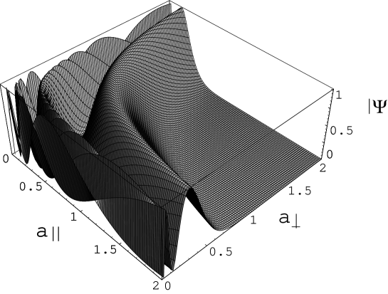
Figure 1: The figure shows the probability density $|\Psi|^{2}$ For the ’physical’ case of a SD3-brane ($p=3$) (with $\mu=0.1$ and $\nu=0.7$) and its variation with respect to the radii $a_{\perp}$ and $a_{\parallel}$. The maxima of the quantum solution $\Psi$ determines a trajectory in the $a_{\perp}-a_{\parallel}$ plane. These maxima satisfy an inverse relation between both radii as shown in Eq. (27).

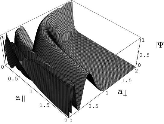
Figure 2: The probability density $|\Psi|^{2}$ (also with $\mu=0.1$ and $\nu=0.7$) for one extreme case with $p=1$. The solution shows that for this case, the maxima of $|\Psi|^{2}$ determines an evolution which is almost projected on the axis $a_{\perp}$, that is, for large values of $a_{\perp}$ it is almost independent on $a_{\parallel}$.

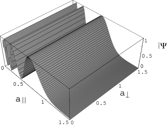
Figure 3: The figure corresponds with the other extreme case with $p=8$ which shows that the probability density $|\Psi|^{2}$ is independent on $a_{\perp}$. This corresponds with a wave function $\Psi$ describing an evolution whose maxima are localized around fixed values of $a_{\parallel}$.

Let us now consider the next leading order of the approximation of the hamiltonian (14), in which $V^{2}(T)$ is neglected with respect to the $V(T)$ or $\mathcal{F}(T)$. As we mentioned in the introduction, this approximation corresponds to the first order correction from the late-time decoupling limit with $T$ still large but nonvanishing $V(T)$ and $f(T)$. This configuration was considered previously by Sen in Refs. senfour ; senfive ; sentime . In this case we have,

$$H_{0} =2e^{\phi/4}P_{T}-\frac{1}{144}e^{-9\beta_{1}}P_{1}^{2}+\frac{9e^{-9\beta_{1}}}{2(p+1)(8-p)}P_{2}^{2}+e^{-9\beta_{1}}P_{\phi}^{2}+(p+2)!e^{-(9\beta_{1}+a\phi)}P_{C}^{2}$$

$$-2\lambda e^{\phi/4}e^{(8-p)\left[\beta_{1}-\frac{1}{9}(p+1)\beta_{2}\right]-\frac{\alpha T}{2}}C=0.$$ (28)

After quantization, we obtain from this hamiltonian again a Schrödinger equation, now with a time dependent potential for the RR field. It is interesting to note that in this case, the term coming from the RR coupling still allows to interpret the tachyon field as time, because its moment still appears linearly, but in this case Eq. (28) leads to a Schrödinger equation with a time-dependent potential. Of course in the absence of RR and dilaton fields, the tachyon field is coupled only to gravity and we recover the situation discussed by Sen in Refs. senfour ; senfive ; sentime .

One way to solve equation (28), could be by traying the time-dependent term as a perturbation. In this case we could look for a solution of the form,

$$\Psi(T,\beta_{1},\beta_{2},C)=\psi(T,\beta_{1},\beta_{2},C)+e^{-\frac{\alpha T}{2}+\frac{i}{2}\mu g_{S}^{1/4}T}\psi_{1}(\beta_{1},\beta_{2},C).$$ (29)

However, when substituted into (28), it gives an equation for $\psi_{1}$ too complicated for an exact solution. The probability density obtained from (29) $|\Psi|^{2}\simeq|\psi|^{2}+2{\rm Re}[\,e^{-\frac{1}{2}(\alpha-i\mu g_{S}^{1/4})T}\overline{\psi}\psi_{1}]$, contains time dependent interference terms corresponding to interactions of the tachyon matter (open strings) with background fields (closed strings). This interference represents a manifestation of the quantum backreaction of the tachyon field by the background.

V Inclusion of electromagnetic fields

We want to see in this section how the tachyon dynamics is modified in the presence of electromagnetic fields. Let us consider the case in which electric and magnetic fields $f_{\alpha\beta}$ are included. The brane action $S_{Brane}$ from Eq. (3) is modified as follows senmuk ; roy ; rey ,

$$S_{Brane}=\frac{\Lambda}{16\pi G_{10}}\int d^{p+2}x_{\parallel}\widehat{\varrho}_{\perp}\left(-V(T)e^{-\phi}\sqrt{-{\cal A}}\text{ }\right)+\frac{\Lambda}{16\pi G_{10}}\int\widehat{\varrho}_{\perp}\mathcal{F(}T\mathcal{)}dT\wedge C_{p+1}\wedge e^{f},$$ (30)

where now the tachyon metric is ${\cal A}_{\alpha\beta}=g_{\alpha\beta}e^{\phi/2}+\partial_{\alpha}T\partial_{\beta}T+f_{\alpha\beta}$ and $f=f_{\alpha\beta}dx^{\alpha}\wedge dx^{\beta}$. For simplicity, we will consider only one nonvanishing component for the electric and magnetic fields, $E=f_{01}=\partial_{0}A_{1}$ and $B=f_{12}=-\partial_{2}A_{1}$. With this choice, the exponential $e^{f}$ in the last term of action (30) contributes only with a factor one. This can be obtained by direct calculation or following peetone , taking into account the ansatz $ISO(p+1)\times SO(8-p,1)$. After integration of the space coordinates, we get the Lagrangian

$$L_{brane}=\lambda e^{(8-p)\left[\beta_{1}-\frac{1}{9}(p+1)\beta_{2}\right]}\mathcal{F}(T)\dot{T}C$$

$$-\lambda\,e^{9\beta_{1}-a\phi/2}\,V(T)\left[\bigg{(}N^{2}e^{\phi/2}-\dot{T}^{2}\bigg{)}\bigg{(}1+e^{-2\left(\beta_{1}+\frac{8-p}{9}\beta_{2}+\phi/4\right)}B^{2}\bigg{)}-E^{2}\right]^{1/2}.$$ (31)

Making the same procedure of introducing a Lagrange multiplier $\Omega$ we found in the late-time limit ($V(T)\rightarrow 0$ as $\left|T\right|\rightarrow\infty$) that the relevant part of the hamiltonian turns out to be,

$$H_{\begin{subarray}{c}brane\\ \left|T\right|\rightarrow\infty\end{subarray}}=2e^{\phi/4}\left[\left(1+e^{-2\left(\beta_{1}+\frac{8-p}{9}\beta_{2}+\phi/4\right)}B^{2}\right)P_{T}^{2}+\Pi^{2}\right]^{1/2},$$ (32)

where $\Pi$ is the momentum conjugated to $A_{1}$. From this expression, we see that the tachyon would decouple only if $\Pi$ vanishes. Thus, under the presence of electromagnetic fields, the tachyon cannot be identified with time in the sense of a Schrödinger-type equation even in the late-time limit.

VI Conclusions

In this work, we have provided an exact solution to the canonical quantization of the SD$p$-brane model gs ; buchelone ; peettwo ; bucheltwo ; peetone . For this effective action, a Wheeler-deWitt equation has been obtained from the hamiltonian analysis. Following Ref. tseytlin , the square root in the tachyonic matter action (10) was eliminated by the introduction of a Lagrange multiplier $\Omega$. From the resulting action the Hamiltonian (14) has been computed and the decoupling late-time limit ($\left|T\right|\rightarrow\infty$) has been done. Even though we have considered the canonical quantization of the effective action with a maximally symmetric metric (4), the quantum version of this field theory and in particular of the model under consideration is interesting on its own right sentime . Moreover, it could provide some insight on string theory beyond the classical limit.

Further we show that the proposal by Sen, concerning the interpretation of the tachyon as time, in the late-time decoupling limit, is valid for this model. In this limit we find an exact wave function for the corresponding Schrödinger equation. The associated probability density is a finite and continuous function of the radii $a_{\parallel}$ and $a_{\perp}$, it shows (a non-singular) continuum of maxima along a definite trajectory, in such a way that if the mean value of one of the radii increases, the mean value of the other one decreases, as shown in Figure 1 for $p=3$ and in Figure 2 and Figure 3 for the extreme cases of $p=1$ and $p=8$, respectively. We have also considered the situation beyond the late-time decoupling limit in which still $T$ is large but $V(T)$ and $f(T)$ are nonvanishing. The coupling of the tachyon with the RR fields allows us still to interpret the tachyon as time. However in this case the Wheeler-deWitt equation (28) leads to a Schrödinger equation with a time-dependent potential. This situation has been already discussed in Refs. senfour ; senfive ; sentime at the classical level. If quantum corrections of the string theory have to be taken into account and if the open-closed duality holds (see remarks of review, revsen ), it would be very interesting to explore if solutions of the Schrödinger equation (28), or its generalizations (representing open-closed states), correspond to a description (at the lowest level) of the physics of the quantum string theory associated to SD$p$-branes.

Finally, we have also shown that in the presence of electromagnetic fields, the interpretation of the tachyon as time seems to be spoiled. Indeed, as can be seen from Eq. (32) that even in the late-time limit the tachyon does not decouple from the electric field.

Acknowledgments

This work was supported in part by CONACyT México Grants Nos. 37851E and 41993F, PROMEP and Gto. University Projects.

References

- (1) A. Sen, “Non-BPS States and Branes in String Theory”, Published in Cargese 1999, Progress in string theory and M-theory, pp 187-234, hep-th/9904207.
- (2) M. Gutperle and A. Strominger, “Spacelike Branes” JHEP 0204 (2002) 018, hep-th/0202210.
- (3) N. Lambert, H. Liu and J. Maldacena, hep-th/0303139.
- (4) D. Gaiotto, N. Itzhaki and L. Rastelli, Nucl. Phys. B 688 (2004) 70, hep-th/0304192.
- (5) A. Sen, Phys. Rev. D 68 (2003) 106003, hep-th/0305011; Phys. Rev. Lett. 91 (2003) 181601, hep-th/0306137.
- (6) A. Sen, “Open Closed Duality: Lessons from Matrix Model”, Mod. Phys. Lett. A 19 (2004) 841, hep-th/0308068.
- (7) M.R. Garousi, Nucl. Phys. B 584 (2000) 284; E.A. Bergshoeff, M. de Roo, T.C. de Wit, E. Eyras and S. Panda, JHEP 0005 (2000) 009; J. Kluson, Phys. Rev. D 62 (2000) 126003; G.W. Gibbons, K. Hori and P. Yi, Nucl. Phys. B 596 (2001) 136.
- (8) A. Sen, “Rolling Tachyon”, JHEP 0204 (2002) 048, hep-th/0203211.
- (9) A. Sen, “Tachyon Matter”, JHEP 0207 (2002) 065, hep-th/0203265.
- (10) A. Sen, “Field Theory of Tachyon Matter”, Mod. Phys. Lett. A 17 (2002) 1797, hep-th/0204143.
- (11) A. Sen, “Time and Tachyon”, Int. J. Mod. Phys. A 18 (2003) 4869, hep-th/0209122.
- (12) F. Quevedo, “Lectures on String/Brane Cosmology”, Class. Quant. Grav. 19 (2002) 5721, hep-th/0210292.
- (13) A. Sen, “Remarks on Tachyon Driven Cosmology”, Talk at Nobel Symposium on Cosmology and String Theory and IIT Kanpur workshop on String Theory, hep-th/0312153.
- (14) G.W. Gibbons, “Cosmological Evolution of the Rolling Tachyon”, Phys. Lett. B 537 (2002) 1, hep-th/0204008.
- (15) G.W. Gibbons, “Thoughts of Tachyon Cosmology”, Class. Quant. Grav. 20 (2003) S321, hep-th/0301117.
- (16) C.-M. Chen, D.V. Galtsov and M. Gutperle, “S-branes Solutions in Supergravity Theories , Phys. Rev. D 66 (2002) 024043, hep-th/0204071.
- (17) M. Kruczenski, R.C. Myers and A.W. Peet, JHEP 0205 (2002) 039, hep-th/0204144.
- (18) F. Quevedo, G. Tasinato and I. Zavala C., “-branes, Negative Tension Branes and Cosmology”, hep-th/0211031.
- (19) A. Buchel, P. Langfelder and J. Walcher, “Does the Tachyon Matter?”, Annals Phys. 302 (2002) 78, hep-th/0207235; A. Buchel and J. Walcher, “The Tachyon does Matter”, Fortsch. Phys. 51 (2003) 885, hep-th/0212150.
- (20) F. Leblond and A.W. Peet, “SD-brane Gravity Fields and Rolling Tachyons”, JHEP 0304 (2003) 048, hep-th/0303035.
- (21) A. Buchel and J. Walcher, “Comments on Supergravity Description of S-branes”, JHEP 0305 (2003) 069, hep-th/0305055.
- (22) F. Leblond and A.W. Peet, “A Note on the Singularity Theorem for Supergravity SD-branes”, JHEP 0404 (2004) 022, hep-th/0305059.
- (23) F. Leblond, “Mirage Resolution of Cosmological Singularities”, hep-th/0403221.
- (24) G.W. Gibbons, K. Hashimoto and P. Yi, “Tachyon Condensates, Carrollian Contraction of Lorentz Group, and Fundamental Strings”, JHEP 0209 (2002) 061, hep-th/0209034.
- (25) A.A. Tseytlin, Nucl. Phys. B 469 (1996) 51.
- (26) K.V. Kuchar, “Time and Interpretations in Quantum Gravity”, in proceedings of the 4th conference on General Relativity and Relativistic Astrophysics, eds G. Kunstatter, D. Vincent and J. Williams (World Scientific, Singapore 1992).
- (27) P. Mukhopadhyay and A. Sen, JHEP 0211 (2002) 047, hep-th/0208142.
- (28) S. Bhattacharya, S. Mukherji and S. Roy, “On the Effective Action of Space-like Brane”, Phys. Lett. B 584 (2004) 163, hep-th/0308069.
- (29) S.-J. Rey and S. Sugimoto, “Rolling Tachyon with Electric and Magnetic Fields- T-duality Approach-”, Phys. Rev. D 67 (2003) 086008, hep-th/0301049.