Noncommutative Correction to the Aharonov-Bohm Scattering: a Field Theory Approach

Abstract

We study a noncommutative nonrelativistic theory in 2+1 dimensions of a scalar field coupled to the Chern-Simons field. In the commutative situation this model has been used to simulate the Aharonov-Bohm effect in the field theory context. We verified that, contrarily to the commutative result, the inclusion of a quartic self-interaction of the scalar field is not necessary to secure the ultraviolet renormalizability of the model. However, to obtain a smooth commutative limit the presence of a quartic gauge invariant self-interaction is required. For small noncommutativity we fix the corrections to the Aharonov-Bohm scattering and prove that up to one-loop the model is free from dangerous infrared/ultraviolet divergences.

I Introduction

Noncommutative field theories present a series of unusual and intriguing properties (see Douglas for some reviews). From a conceptual standpoint the inherent nonlocality of these theories lead to an entanglement of scales so that some ultraviolet (UV) divergences of their commutative counterparts appear as infrared (IR) singularities. In general they are damaging to the perturbative expansions although in some supersymmetric models gomes2 ; bichl ; gomes3 they could be under control. Noncommutative field theories have also been used to clarify condensed matter phenomena as the fractional Hall susskind and Aharonov-Bohm (AB) chaichian ; Gamboa effects.

In the context of nonrelativistic quantum mechanics, previous study on the noncommutative AB effect have shown that, in contrast with the commutative situation, the cross section for the scattering of scalar particles by a thin solenoid does not vanish even when the magnetic field assumes certain discrete values Gamboa .

In this work we will proceed further the investigations on the changes on the AB effect due to the noncommutativity of the space. In our study the effect will be simulated by a nonrelativistic field theory describing spin zero particles interacting through a Chern-Simons (CS) field. It is worth to recall that in the commutative scenario, to cancel ultraviolet divergences and to obtain accordance with the exact result, it was necessary to introduce a quartic self-interaction for the scalar field lozano . This result was reobtained by considering the low momentum limit of the full relativistic theory boz . Even in the case of U(1) gauge symmetry to which we will restrict our considerations, due to the noncommutativity, the CS field is similar to a non-Abelian gauge field so that we will be actually dealing with a non-Abelian AB effect lee (see bergman for studies on the non-Abelian commutative AB effect using the CS field). Besides, because of the change in the character of some divergences, from ultraviolet to infrared, the renormalizability of the model may be in jeopardy. However, in the present situation there are two possible orderings for the quartic self-interactions. There is one more free parameter and this could help to formulate a consistent model. In any case, as the limit of small noncommutativity is singular, features different from those in Gamboa emerge from our analysis.

In this work all calculations are performed in the Coulomb gauge which for nonrelativistic studies seems to be more adequate. We show that up to the one-loop order the UV divergences of the planar contributions are canceled in the calculation of the four-point function and, contrary to the commutative case, do not have a conformal anomaly. Hence, the planar part is renormalizable without the contact interaction needed in the commutative situation. Nevertheless, as mentioned before, the nonplanar part presents logarithmic infrared divergences as the noncommutative parameter tends to zero. To eliminate these divergences we introduce in the Lagrangian quartic interactions of the type $\frac{\lambda_{1}}{8}[\phi,\phi^{\dagger}]_{\ast}\ast[\phi,\phi^{\dagger}]_{\ast}$ and $\frac{\lambda_{2}}{8}\{\phi,\phi^{\dagger}\}_{\ast}\ast\{\phi,\phi^{\dagger}\}_{\ast}$, all field products being Moyal ones. For general values of $\lambda_{1}$ and $\lambda_{2}$ gauge invariance will be broken and UV divergences originated from the quartic terms occur. However, it turns out that, for the special values $\lambda_{1}=\lambda_{2}=\lambda$, for which the action is gauge invariant, these UV divergences are eliminated. We prove then that IR divergences in the scattering amplitude disappear for special values of the coupling constant $\lambda$.

The paper is organized as follows. In section II, we introduce the model, present its Coulomb gauge Feynman rules and discuss some aspects of the renormalization program for the model. In section III, we compute the particle-particle scattering up to order one-loop. We calculate the scattering amplitude by separating the planar and nonplanar parts and complete the one-loop analysis of the IR/UV divergences initiated in the previous section. Some integrals needed in the calculations are collected in the Appendix. Final comments are made in the Conclusions.

II Noncommutative Perturbative Theory

We consider the noncommutative version of the theory of a nonrelativistic scalar field coupled with a CS field in 2+1 dimensions described by the action

$$S[A,\phi] = \int d^{3}x\left[\frac{\kappa}{2}\varepsilon^{\mu\nu\lambda}\left(A_{\mu}\ast\partial_{\nu}A_{\lambda}+\frac{2ig}{3}A_{\mu}\ast A_{\nu}\ast A_{\lambda}\right)-\frac{1}{2\xi}\partial_{i}A^{i}\ast\partial_{j}A^{j}\right.$$ (1)

$$+\left.i\phi^{\dagger}\ast D_{t}\phi-\frac{1}{2m}(\mathbf{D}\phi)^{\dagger}\ast(\mathbf{D}\phi)-\frac{\lambda_{1}}{8}[\phi,\phi^{\dagger}]_{\ast}\ast[\phi,\phi^{\dagger}]_{\ast}\right.$$

$$-\left.\frac{\lambda_{2}}{8}\{\phi,\phi^{\dagger}\}_{\ast}\ast\{\phi,\phi^{\dagger}\}_{\ast}+\partial^{i}\bar{c}\ast\partial_{i}c+ig\partial^{i}\bar{c}\ast[A_{i},c]\right],$$

where a Coulomb gauge fixing and the corresponding Faddeev-Popov terms are already included. The fields $\phi$ and $\phi^{\dagger}$ belong to the fundamental representation of the $U(1)$ gauge group

$$\phi\rightarrow(e^{i\Lambda})_{\ast}\ast\phi,$$ (2)

$$\phi^{\dagger}\rightarrow\phi^{\dagger}\ast(e^{-i\Lambda})_{\ast},$$ (3)

whereas the gauge field transforms as

$$A_{\mu}\rightarrow({\textrm{e}}^{i\Lambda})_{\ast}\ast A_{\mu}\ast({\textrm{e}}^{-i\Lambda})_{\ast}+i[\partial_{\mu}({\textrm{e}}^{i\Lambda})_{\ast}]\ast({\textrm{e}}^{-i\Lambda})_{\ast}.$$ (4)

The covariant derivatives are given by

$$D_{t}\phi = \partial_{t}\phi+igA_{0}\ast\phi,$$

$$D_{i}\phi = \partial_{i}\phi+igA_{i}\ast\phi.$$ (5)

Notice that there are two different orderings for the quartic self-interaction. In (1) they were written in terms of Moyal commutators and anticommutators of the scalar fields.

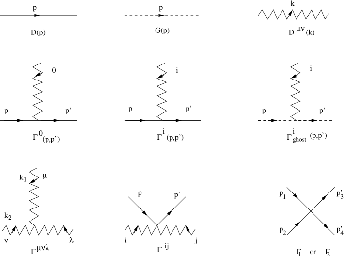
Figure 1: Feynman rules for the action (1).

For convenience, we will work in a strict Coulomb gauge obtained by letting $\xi\rightarrow 0$. Furthermore, we will use a graphical notation where the CS field, the matter field and the ghost field propagators are represented by wavy, continuous and dashed lines respectively. The graphical representation for the Feynman rules is given in Fig. 1 and the corresponding analytical expression are:

(i) The matter field propagator:

$$D(p)=\frac{i}{p_{0}-\frac{\mathbf{p}^{2}}{2m}+i\epsilon},$$ (6)

(ii) The ghost field propagator:

$$G(p)=-\frac{i}{\mathbf{p}^{2}},$$ (7)

(iii) The gauge field propagator in the limit $\xi\rightarrow 0$ is

$$D_{\mu\nu}(k)=\frac{\varepsilon_{\mu\nu\lambda}\bar{k}^{\lambda}}{\kappa\mathbf{k}^{2}},$$ (8)

where $\bar{k}^{\lambda}$=$(0,{\bf k})$.

(iv) The analytical expressions associated with the vertices are:

$$\Gamma^{0}(p,p^{\prime})=-ige^{ip\theta p^{\prime}},$$ (9)

$$\Gamma^{i}(p,p^{\prime})=\frac{ig}{2m}(p+p^{\prime})^{i}e^{ip\theta p^{\prime}},$$ (10)

$$\Gamma^{i}_{ghost}(p,p^{\prime})=-2gp^{\prime i}\sin(p\theta p^{\prime}),$$ (11)

$$\Gamma^{\mu\nu\lambda}(k_{1},k_{2})=2ig\kappa\varepsilon^{\mu\nu\lambda}\sin(k_{1}\theta k_{2}),$$ (12)

$$\Gamma^{ij}(k_{1},k_{2},p,p^{\prime})=-\frac{ig^{2}}{m}\cos(k_{1}\theta k_{2})e^{ip\theta p^{\prime}}\delta^{ij},$$ (13)

$$\Gamma_{1}(p_{1},p_{3}^{\prime},p_{2},p_{4}^{\prime})=i\lambda_{1}[\sin(p_{1}\theta p_{3}^{\prime})\sin(p_{2}\theta p_{4}^{\prime})+\sin(p_{1}\theta p_{4}^{\prime})\sin(p_{2}\theta p_{3}^{\prime})],$$ (14)

$$\Gamma_{2}(p_{1},p_{3}^{\prime},p_{2},p_{4}^{\prime})=-i\lambda_{2}[\cos(p_{1}\theta p_{3}^{\prime})\cos(p_{2}\theta p_{4}^{\prime})+\cos(p_{1}\theta p_{4}^{\prime})\cos(p_{2}\theta p_{3}^{\prime})].$$ (15)

In these expressions we have defined $k_{1}\theta k_{2}\equiv\frac{1}{2}\theta^{\mu\nu}k_{1\mu}k_{2\nu}$, where $\theta^{\mu\nu}$ is the anti-symmetric matrix which characterize the noncommutativity of the underlying space. For simplicity we assume that $\theta^{0i}=0$ and $\theta^{ij}=\theta\epsilon^{ij}$ with $\epsilon^{ij}$ being the two dimensional Levi-Cività symbol, normalized as $\epsilon^{12}=1$.

In the one-loop approximation there are quadratic divergences, associated with the two point functions of the gauge and scalar fields, linear divergences, associated with the scalar field four point function and logarithmic divergences, associated with the three point functions $<A_{\mu}\phi\phi^{\dagger}>$. In the sequel we shall analyze each one of these divergences.

(1) Gauge and scalar fields two-point functions. The graph in Fig. 2$a$ which contributes to the gauge field two point function is planar so that it can be eliminated by an adequate counterterm. Specifically, the only one-loop nonvanishing contribution is given by

$$\Pi_{a}^{ij} = -\frac{ig^{2}\delta^{ij}}{2m}\int\frac{d^{2}{\bf{k}}}{(2\pi)^{2}}=-\frac{ig^{2}\delta^{ij}\Lambda^{2}}{8\pi m}.$$ (16)

This is a gauge noninvariant term and shall be removed by a $A_{i}A_{i}$ counterterm so that gauge (BRST) invariance remains unbroken.

The diagram in Fig 2$b$ which contributes to the scalar field two-point function have both planar and nonplanar parts. As before, the planar part can be eliminated by a counterterm. For general values of $\lambda_{1}$ and $\lambda_{2}$ , the nonplanar part although ultraviolet finite may generate nonintegrable infrared singularities. These nonplanar parts are however canceled if one chooses $\lambda_{1}=\lambda_{2}$ which is also the condition to enforce gauge invariance.

(2) As Lorentz invariance is broken, the three point function $<TA_{\mu}\phi\phi^{\dagger}>$ presents two types of divergences:

(a) The one-loop contribution to $<TA_{0}\phi\phi^{\dagger}>$, drawn in Fig. 3$a$ is given by

$$\Gamma^{0} =- \frac{g^{3}e^{ip\theta p^{\prime}}}{2\kappa}\lim_{\mu\rightarrow 0}\int\frac{d^{2}{\bf{k}}}{(2\pi)^{2}}\frac{({\bf{q}}\wedge{\bf{k}})[1-e^{-2iq\theta k}]}{{\bf{k}}^{2}[({\bf{k}}-{\bf{q}})^{2}+\mu^{2}]},$$ (17)

where we introduced the parameter $\mu$ to regulate possible infrared divergences in the intermediary steps of the calculation. For small $\theta$ we obtain

$$\Gamma^{0} = \frac{ig^{3}\theta{\bf{q}}^{2}e^{ip\theta p^{\prime}}}{8\pi\kappa}\left[\ln\left(\frac{\theta{\bf{q}}^{2}}{2}\right)+\gamma-1\right],$$ (18)

where $\gamma$ is the Euler-Mascheroni constant. Notice that $\Gamma^{0}$ is finite in the infrared limit.

(b) Concerning the three point function $<TA^{i}\phi\phi^{\dagger}>$, we found two contributions

$$\Gamma^{i}_{1}=\frac{g^{3}e^{ip\theta p^{\prime}}}{2m\kappa}\lim_{\mu\rightarrow 0}\int\frac{d^{2}{\bf{k}}}{(2\pi)^{2}}\frac{[({\bf{p}}-{\bf{k}})\wedge{\bf{p}}^{\prime}][1-e^{-2iq\theta k}]}{{\bf{k}}^{2}[({\bf{k}}-{\bf{q}})^{2}+\mu^{2}]}k^{i},$$ (19)

$$\Gamma^{i}_{2}=-\frac{g^{3}e^{ip\theta p^{\prime}}}{2m\kappa}\lim_{\mu\rightarrow 0}\int\frac{d^{2}{\bf{k}}}{(2\pi)^{2}}\frac{({\bf{p}}\wedge{\bf{k}})[1-e^{-2iq\theta k}]}{{\bf{k}}^{2}[({\bf{k}}-{\bf{q}})^{2}+\mu^{2}]}(k^{i}-q^{i}),$$ (20)

associated with the graphs in the Figs. 3$b$ and 3$c$, respectively. For small $\theta$ the calculation of these amplitudes furnishes the following results for their planar and nonplanar parts

(b1) Planar parts:

$$\Gamma^{i}_{planar\,1}=-\frac{g^{3}e^{ip\theta p^{\prime}}}{8\pi m\kappa}\left\{q^{i}\frac{{\bf{p}}\wedge{\bf{p}}^{\prime}}{{\bf{q}}^{2}}\ln\left(\frac{\mu^{2}}{{\bf{q}}^{2}}\right)+\varepsilon^{in}p^{\prime{n}}\left[\ln\left(\frac{\mu^{2}}{\Lambda^{2}}\right)-2\right]\right\},$$ (21)

$$\Gamma^{i}_{planar\,2}=-\frac{g^{3}e^{ip\theta p^{\prime}}}{8\pi m\kappa}\varepsilon^{in}p^{n}\left[\ln\left(\frac{\Lambda^{2}}{{\bf{q}}^{2}}\right)+2\right].$$ (22)

(b2) Nonplanar parts:

$$\!\!\!\!\!\Gamma^{i}_{nplanar\,1} = \frac{g^{3}e^{ip\theta p^{\prime}}}{8\pi m\kappa}\left\{({\bf{p}}\wedge{\bf{p}}^{\prime})\left[\frac{q^{i}}{{\bf{q}}^{2}}\ln\left(\frac{\mu^{2}}{{\bf{q}}^{2}}\right)-i{\tilde{q}}^{i}\left(\ln\left(\frac{\theta{\bf{q}}^{2}}{2}\right)+\gamma-1\right)\right]\right.$$ (23)

$$+\left.\varepsilon^{in}p^{\prime{n}}\left[\ln\left(\frac{\mu^{2}}{{\bf{q}}^{2}}\right)+\ln\left(\frac{\theta{\bf{q}}^{2}}{2}\right)+1+\gamma\right]\right\},$$

$$\!\!\!\!\!\Gamma^{i}_{nplanar\,2} = \!\!-\frac{g^{3}e^{ip\theta p^{\prime}}}{8\pi m\kappa}\left\{[\varepsilon^{in}p^{n}\!+i\theta q^{i}({\bf{p}}.{\bf{q}})]\left[\ln\left(\frac{\theta{\bf{q}}^{2}}{2}\right)\!+\gamma\right]\!+\![\varepsilon^{in}p^{n}-i\theta q^{i}({\bf{p}}.{\bf{q}})]\right\}\!,$$ (24)

where we have defined ${\tilde{q}}^{i}\equiv\theta^{ij}q_{j}$.

Summing up these parts we get the total contribution for small $\theta$

$$\Gamma^{i} = \Gamma^{i}_{planar}+\Gamma^{i}_{nplanar}$$ (25)

$$= -\frac{ig^{3}e^{ip\theta p^{\prime}}}{8\pi m\kappa}[{\tilde{q}}^{i}({\bf{p}}\wedge{\bf{p}}^{\prime})+\theta q^{i}({\bf{p}}.{\bf{q}})]\left[\ln\left(\frac{\theta{\bf{q}}^{2}}{2}\right)+\gamma-1\right]$$

$$-\frac{g^{3}e^{ip\theta p^{\prime}}\varepsilon^{in}q^{n}}{8\pi m\kappa}\left[\ln\left(\frac{\Lambda^{2}\theta}{2}\right)+\gamma+3\right].$$

Notice that the final results do not depend on $\mu$. The infrared divergences being only logarithmic are harmless whereas the ultraviolet divergence has to be eliminated by a counterterm. It remains to analyze the four point function but that will be done in the next section together with the computation of the two body scattering matrix.

III Particle-Particle Scattering

The object that we wish to analyze is the four point function associated with the scattering of two identical particles in the center-of-mass frame. The relevant diagrams are depicted in Figs. 4 and 5 but for sake of simplicity we have drawn only the $s$-channel processes. In the tree approximation the gauge part of the two body scattering amplitude is given by (see Fig. 4$a$),

$${\cal{A}}_{a}^{0}(\varphi)=-\frac{2ig^{2}({\bf{p}}_{1}\wedge{\bf{p}}_{3})}{m\kappa}\left[\frac{e^{i(p_{1}\theta p_{3}+p_{2}\theta p_{4})}}{({\bf{p}}_{1}-{\bf{p}}_{3})^{2}}-\frac{e^{-i(p_{1}\theta p_{3}+p_{2}\theta p_{4})}}{({\bf{p}}_{1}+{\bf{p}}_{3})^{2}}\right],$$ (26)

where ${\bf{p}}_{1}$, ${\bf{p}}_{2}$ and ${\bf{p}}_{3}$, ${\bf{p}}_{4}$ are the incoming and outgoing momenta. Since $\theta_{ij}=\theta\varepsilon_{ij}$, the phase is

$$p_{1}\theta p_{3}+p_{2}\theta p_{4}=\theta({\bf{p}}_{1}\wedge{\bf{p}}_{3})=\theta{\bf{p}}^{2}\sin\varphi=\bar{\theta}\sin\varphi,$$ (27)

where we have defined $\bar{\theta}\equiv\theta{\bf{p}}^{2}$, ${\bf{p}}^{2}\equiv{\bf{p}}^{2}_{1}={\bf{p}}^{2}_{3}$ and $\varphi$ is the scattering angle. Therefore, Eq. (26) can be rewritten as

$${\cal{A}}_{a}^{0}(\varphi)=-\frac{ig^{2}}{m\kappa}\left[\frac{e^{i\bar{\theta}\sin\varphi}}{1-\cos\varphi}-\frac{e^{-i\bar{\theta}\sin\varphi}}{1+\cos\varphi}\right]\sin\varphi,$$ (28)

which for small $\bar{\theta}$ gives ${\cal{A}}_{a}^{0}(\varphi)\approx-\frac{2ig^{2}}{m\kappa}(\cot\varphi+i\bar{\theta}$).

By taking into account the quartic self-interaction we have the additional contribution

$${\cal{A}}_{b}^{0}(\varphi) = \lambda_{1}[\sin(p_{1}\theta p_{3})\sin(p_{2}\theta p_{4})+\sin(p_{1}\theta p_{4})\sin(p_{2}\theta p_{3})]$$ (29)

$$-\lambda_{2}[\cos(p_{1}\theta p_{3})\cos(p_{2}\theta p_{4})+\cos(p_{1}\theta p_{4})\cos(p_{2}\theta p_{3})]$$

$$= 2\lambda_{1}\sin^{2}\left(\frac{\bar{\theta}\sin\varphi}{2}\right)-2\lambda_{2}\cos^{2}\left(\frac{\bar{\theta}\sin\varphi}{2}\right),$$

coming from the graph in Fig. 4$b$. Thus, the full tree level amplitude is

$${\cal{A}}(\varphi) = -\frac{ig^{2}}{m\kappa}\left[\cot\left(\frac{\varphi}{2}\right)e^{i\bar{\theta}\sin\varphi}-\tan\left(\frac{\varphi}{2}\right)e^{-i\bar{\theta}\sin\varphi}\right]$$ (30)

$$+2\lambda_{1}\sin^{2}\left(\frac{\bar{\theta}\sin\varphi}{2}\right)-2\lambda_{2}\cos^{2}\left(\frac{\bar{\theta}\sin\varphi}{2}\right).$$

The one-loop contribution to the scattering amplitude is depicted in the Fig. 5 (all other possible one-loop graphs vanish). The analytic expressions associated with these graphs, after performing the $k_{0}$ integration, are

1. For the triangle graph shown in Fig. 5$a$:

$${\cal{A}}_{a}(\varphi) = -\frac{g^{4}}{4m\kappa^{2}}e^{i(p_{1}\theta p_{3}+p_{2}\theta p_{4})}\int\frac{d^{2}{\bf{k}}}{(2\pi)^{2}}\frac{{\bf{k}}.({\bf{k}}-{\bf{q}})}{{\bf{k}}^{2}({\bf{k}}-{\bf{q}})^{2}}\left[1+e^{-2iq\theta k}\right]$$ (31)

$$+(p_{1}\leftrightarrow p_{2})+(p_{3}\leftrightarrow p_{4})+\left(p_{1}\leftrightarrow p_{2}\quad\mbox{and}\quad p_{3}\leftrightarrow p_{4}\right),$$

where ${\bf{q}}={\bf{p}}_{1}-{\bf{p}}_{3}$ is the momentum transferred,

2. For the trigluon graph shown in Fig. 5$b$ (${\bf{q}}^{\prime}={\bf{p}}_{1}+{\bf{p}}_{3}$):

$${\cal{A}}_{b}(\varphi)={\cal{A}}^{1}_{b}(\varphi)+{\cal{A}}^{2}_{b}(\varphi)+{\cal{A}}^{3}_{b}(\varphi),$$ (32)

where

$${\cal{A}}^{1}_{b}(\varphi) = \frac{g^{4}}{4m\kappa^{2}}e^{i(p_{1}\theta p_{3}+p_{2}\theta p_{4})}\int\frac{d^{2}{\bf{k}}}{(2\pi)^{2}}\left[\frac{{\bf{k}}^{2}{\bf{q}}^{2}-({\bf{k}}.{\bf{q}})^{2}+({\bf{k}}.{\bf{q}}^{\prime})({\bf{k}}.{\bf{q}})-({\bf{k}}.{\bf{q}}^{\prime}){\bf{q}}^{2}}{{\bf{k}}^{2}{\bf{q}}^{2}({\bf{k}}-{\bf{q}})^{2}}\right]$$

$$\times\left[1-e^{-2iq\theta k}\right]+(p_{1}\leftrightarrow p_{2})+(p_{3}\leftrightarrow p_{4})+(p_{1}\leftrightarrow p_{2}\quad\mbox{and}\quad p_{3}\leftrightarrow p_{4}),$$

$${\cal{A}}^{2}_{b}(\varphi) = \frac{g^{4}}{4m\kappa^{2}}e^{i(p_{1}\theta p_{3}+p_{2}\theta p_{4})}\int\frac{d^{2}{\bf{k}}}{(2\pi)^{2}}\left[\frac{{\bf{k}}^{2}{\bf{q}}^{2}-2({\bf{k}}.{\bf{q}})({\bf{k}}.{\bf{p}}_{1})}{{\bf{k}}^{2}{\bf{q}}^{2}({\bf{k}}-{\bf{q}})^{2}}\right]\left[1-e^{-2iq\theta k}\right]$$

$$+(p_{1}\leftrightarrow p_{2})+(p_{3}\leftrightarrow p_{4})+(p_{1}\leftrightarrow p_{2}\quad\mbox{and}\quad p_{3}\leftrightarrow p_{4}),$$

$${\cal{A}}^{3}_{b}(\varphi) = -\frac{g^{4}}{4m\kappa^{2}}e^{i(p_{1}\theta p_{3}+p_{2}\theta p_{4})}\int\frac{d^{2}{\bf{k}}}{(2\pi)^{2}}\left[\frac{({\bf{k}}.{\bf{q}}^{\prime}){\bf{q}}^{2}}{{\bf{k}}^{2}{\bf{q}}^{2}({\bf{k}}-{\bf{q}})^{2}}\right]\left[1-e^{-2iq\theta k}\right]$$ (33)

$$+(p_{1}\leftrightarrow p_{2})+(p_{3}\leftrightarrow p_{4})+(p_{1}\leftrightarrow p_{2}\quad\mbox{and}\quad p_{3}\leftrightarrow p_{4}),$$

3. For the bubble graph shown in Fig. 5$c$:

$${\cal{A}}_{c}(\varphi) = \int\frac{d^{2}{\bf{k}}}{(2\pi)^{2}}\left\{4m(\lambda_{1}-\lambda_{2})^{2}-8m(\lambda_{1}^{2}-\lambda_{2}^{2})\cos(2k\theta p_{1})\right.$$ (34)

$$+\left.2m(\lambda_{1}+\lambda_{2})^{2}[\cos(2k\theta q)+\cos(2k\theta q^{\prime})]\right\}\frac{1}{({\bf{k}}^{2}-{\bf{p}}^{2}-i\epsilon)}.$$

The above integrals being logarithmically divergent need a regularization. Thus, although not indicated, a cutoff regularization is being implicitly assumed.

4. For the box graph in Fig. 5$d$:

$${\cal{A}}_{d}(\varphi)={\cal{A}}_{d}^{1}(\varphi)+{\cal{A}}_{d}^{2}(\varphi),$$ (35)

where

$${\cal{A}}_{d}^{1}(\varphi)=\frac{4g^{4}}{m\kappa^{2}}\int\frac{d^{2}{\bf{k}}}{(2\pi)^{2}}\frac{({\bf{p}}_{1}\wedge{\bf{k}})({\bf{p}}_{3}\wedge{\bf{k}})e^{2iq\theta k}}{({\bf{k}}-{\bf{p}}_{1})^{2}({\bf{k}}-{\bf{p}}_{3})^{2}({\bf{k}}^{2}-{\bf{p}}^{2}-i\epsilon)},$$ (36)

$${\cal{A}}_{d}^{2}(\varphi)=-\frac{4g^{4}}{m\kappa^{2}}\int\frac{d^{2}{\bf{k}}}{(2\pi)^{2}}\frac{({\bf{p}}_{1}\wedge{\bf{k}})({\bf{p}}_{3}\wedge{\bf{k}})e^{-2iq^{\prime}\theta k}}{({\bf{k}}+{\bf{p}}_{1})^{2}({\bf{k}}-{\bf{p}}_{3})^{2}({\bf{k}}^{2}-{\bf{p}}^{2}-i\epsilon)}.$$ (37)

To compute the above integrals, we separate their planar and nonplanar contributions. A simplifying aspect is that the box graph is purely nonplanar.

III.1 Planar Contribution

In the perturbative expansion there is one planar contribution containing phase factors which depend only on the external momenta. Although the interaction induced by the noncommutativity is nonlocal, the divergences in the momentum integration for closed internal loops are the same as for the commutative theory.

The calculations of the planar contributions are standard so that we just list the results:

1. The planar part of the triangle graph,

$${\cal{A}}_{a}^{p}(\varphi) = -\frac{g^{4}}{4m\kappa^{2}}\int\frac{d^{2}{\bf{k}}}{(2\pi)^{2}}\left[\frac{{\bf{k}}.({\bf{k}}-{\bf{q}})e^{i\bar{\theta}\sin\varphi}}{{\bf{k}}^{2}({\bf{k}}-{\bf{q}})^{2}}+\frac{{\bf{k}}.({\bf{k}}+{\bf{q}}^{\prime})e^{-i\bar{\theta}\sin\varphi}}{{\bf{k}}^{2}({\bf{k}}+{\bf{q}}^{\prime})^{2}}\right.$$ (38)

$$+\left.({\bf{q}}\rightarrow-{\bf{q}},\quad{\bf{q}}^{\prime}\rightarrow-{\bf{q}}^{\prime})\right],$$

gives

$${\cal{A}}_{a}^{p}(\varphi) = -\frac{g^{4}}{4\pi m\kappa^{2}}[\cos(\bar{\theta}\sin\varphi)\ln\left(\frac{\Lambda^{2}}{{\bf{p}}^{2}}\right)$$ (39)

$$-\ln|2\sin(\varphi/2)|e^{i\bar{\theta}\sin\varphi}-\ln|2\cos(\varphi/2)|e^{-i\bar{\theta}\sin\varphi}].$$

2. The planar part of the trigluon graph is more intricate being given by

$${\cal{A}}_{b}^{p}(\varphi)={\cal{A}}_{b}^{1p}(\varphi)+{\cal{A}}_{b}^{2p}(\varphi)+{\cal{A}}_{b}^{3p}(\varphi),$$ (40)

where

$${\cal{A}}_{b}^{1p}(\varphi) = \frac{g^{4}}{4m\kappa^{2}}\int\frac{d^{2}{\bf{k}}}{(2\pi)^{2}}\left[\frac{({\bf{k}}^{2}{\bf{q}}^{2}-({\bf{k}}.{\bf{q}})^{2})e^{i\bar{\theta}\sin\varphi}}{{\bf{k}}^{2}{\bf{q}}^{2}({\bf{k}}-{\bf{q}})^{2}}+\frac{({\bf{k}}^{2}{\bf{q}}^{\prime 2}-({\bf{k}}.{\bf{q}}^{\prime})^{2})e^{-i\bar{\theta}\sin\varphi}}{{\bf{k}}^{2}{\bf{q}}^{\prime 2}({\bf{k}}-{\bf{q}}^{\prime})^{2}}\right]$$ (41)

$$+({\bf{q}}\rightarrow-{\bf{q}},\quad{\bf{q}}^{\prime}\rightarrow-{\bf{q}}^{\prime}),$$

$${\cal{A}}_{b}^{2p}(\varphi) = \frac{g^{4}}{4m\kappa^{2}}\int\frac{d^{2}{\bf{k}}}{(2\pi)^{2}}\left[\frac{{\bf{k}}^{2}{\bf{q}}^{2}-2({\bf{k}}.{\bf{q}})({\bf{p}}_{1}.{\bf{k}})}{{\bf{k}}^{2}{\bf{q}}^{2}({\bf{k}}-{\bf{q}})^{2}}e^{i\bar{\theta}\sin\varphi}+\frac{{\bf{k}}^{2}{\bf{q}}^{\prime 2}-2({\bf{k}}.{\bf{q}}^{\prime})({\bf{p}}_{2}.{\bf{k}})}{{\bf{k}}^{2}{\bf{q}}^{\prime 2}({\bf{k}}-{\bf{q}}^{\prime})^{2}}e^{-i\bar{\theta}\sin\varphi}\right]$$ (42)

$$+({\bf{q}}\rightarrow-{\bf{q}},\quad{\bf{q}}^{\prime}\rightarrow-{\bf{q}}^{\prime}),$$

$${\cal{A}}_{b}^{3p}(\varphi) = -\frac{g^{4}}{4m\kappa^{2}}\int\frac{d^{2}{\bf{k}}}{(2\pi)^{2}}\left[\left(\frac{({\bf{k}}.{\bf{q}}^{\prime})}{{\bf{k}}^{2}({\bf{k}}-{\bf{q}})^{2}}-\frac{({\bf{k}}.{\bf{q}}^{\prime})}{{\bf{k}}^{2}({\bf{k}}+{\bf{q}})^{2}}\right)e^{i\bar{\theta}\sin\varphi}\right.$$ (43)

$$+\left.\left(\frac{({\bf{k}}.{\bf{q}})}{{\bf{k}}^{2}({\bf{k}}-{\bf{q}}^{\prime})^{2}}-\frac{({\bf{k}}.{\bf{q}})}{{\bf{k}}^{2}({\bf{k}}+{\bf{q}}^{\prime})^{2}}\right)e^{-i\bar{\theta}\sin\varphi}\right].$$

and the final result is

$${\cal{A}}_{b}^{p}(\varphi) = \frac{g^{4}}{4\pi m\kappa^{2}}[\cos(\bar{\theta}\sin\varphi)\left[\ln\left(\frac{\Lambda^{2}}{{\bf{p}}^{2}}\right)+1\right]$$ (44)

$$-\ln|2\sin(\varphi/2)|e^{i\bar{\theta}\sin\varphi}-\ln|2\cos(\varphi/2)|e^{-i\bar{\theta}\sin\varphi}].$$

Notice now that the sum of the planar contribution, ${\cal{A}}_{a}^{p}(\varphi)$ and ${\cal{A}}_{b}^{p}(\varphi)$, is

$${\cal{A}}_{a+b}^{p}(\varphi)=\frac{g^{4}}{4\pi m\kappa^{2}}\cos(\bar{\theta}\sin\varphi),$$ (45)

so that the divergent parts of these graphs mutually cancel, unlike in the commutative case bergman . Thus, to eliminate the ultraviolet divergences a quartic self-interaction does not seem to be necessary. However, we should be cautious because as remarked before some ultraviolet divergences have been transmuted into infrared ones so that the quartic self-interaction may still be needed.

3. The contribution of planar part of the bubble graph is logarithmically divergent and is equal to

$${\cal{A}}_{c}^{p}(\varphi)=\frac{4m(\lambda_{1}-\lambda_{2})^{2}}{(2\pi)^{2}}\int d^{2}{\bf{k}}\frac{1}{{(\bf{k}}^{2}-{\bf{p}}^{2}-i\epsilon)}=\frac{m(\lambda_{1}-\lambda_{2})^{2}}{\pi}\left[\ln\left(\frac{\Lambda^{2}}{{\bf{p}}^{2}}\right)+i\pi\right].$$ (46)

We can get rid of the divergence by setting $\lambda_{1}=\lambda_{2}=\lambda$. The total planar part of the amplitude is therefore

$${\cal{A}}_{\mbox{1-loop}}^{p}(\varphi) = -\frac{ig^{2}}{m\kappa}[\cot(\varphi/2)e^{i\bar{\theta}\sin\varphi}-\tan(\varphi/2)e^{-i\bar{\theta}\sin\varphi}]$$ (47)

$$-2\lambda\cos(\bar{\theta}\sin\varphi)+\frac{g^{4}}{4\pi m\kappa^{2}}\cos(\bar{\theta}\sin\varphi),$$

furnishing up to first order in the parameter $\bar{\theta}$,

$${\cal{A}}_{\mbox{1-loop}}^{p}(\varphi) = -\frac{ig^{2}}{m\kappa}\left[\cot\left(\frac{\varphi}{2}\right)-\tan\left(\frac{\varphi}{2}\right)+i\bar{\theta}\sin\varphi\left[\cot\left(\frac{\varphi}{2}\right)+\tan\left(\frac{\varphi}{2}\right)\right]\right]$$ (48)

$$-2\lambda+\frac{g^{4}}{4\pi m\kappa^{2}},$$

$$= -\frac{i2g^{2}}{m\kappa}\left[\cot\varphi+i\bar{\theta}\right]-2\lambda+\frac{g^{4}}{4\pi m\kappa^{2}}.$$

III.2 Nonplanar Contribution

The nonplanar contributions are given by terms which contain extra phase factors depending on the internal (loop) momenta. For the graphs (5$a$) these contributions are

$${\cal{A}}_{a}^{np}(\varphi) = -\frac{g^{4}}{4m\kappa^{2}}e^{i\bar{\theta}\sin\varphi}\int\frac{d^{2}{\bf{k}}}{(2\pi)^{2}}\frac{{\bf{k}}.({\bf{k}}-{\bf{q}})}{{\bf{k}}^{2}({\bf{k}}-{\bf{q}})^{2}}e^{-2iq\theta k}$$ (49)

$$+(p_{1}\leftrightarrow p_{2})+(p_{3}\leftrightarrow p_{4})+(p_{1}\leftrightarrow p_{2}\quad\mbox{and}\quad p_{3}\leftrightarrow p_{4}),$$

Let us begin by computing the first term in the r.h.s. of the above expression. This is done straightforwardly by using Feynman parameterization and the result Gel

$$\int\frac{d^{n}k}{(2\pi)^{n}}\frac{e^{ik_{\alpha}\tilde{p}^{\alpha}}}{[k^{2}-M^{2}]^{\lambda}}=i(-1)^{\lambda}\frac{M^{n/2-\lambda}}{2^{\lambda-1}(2\pi)^{n/2}\Gamma[\lambda]}\frac{K_{n/2-\lambda}\left(\sqrt{-M^{2}{\tilde{p}}^{2}}\right)}{(-{\tilde{p}^{2}})^{n/2-\lambda}},$$ (50)

where $K_{\nu}$ is the modified Bessel function of order $\nu$. Proceeding in this way we obtain

$${\cal{A}}_{a1}^{np}(\varphi)=-\frac{g^{4}}{4\pi m\kappa^{2}}\int_{0}^{1}dx\left[K_{0}(\sqrt{a^{2}\bar{\theta}^{2}})-\sqrt{a^{2}\bar{\theta}^{2}}K_{1}(\sqrt{a^{2}\bar{\theta}^{2}})\right]e^{i\bar{\theta}\sin\varphi},$$ (51)

where $a^{2}=16x(1-x)\sin^{4}(\varphi/2)$. Collecting this with the results for the other terms then provides

$${\cal{A}}_{a}^{np}(\varphi) = -\frac{g^{4}}{4\pi m\kappa^{2}}\int_{0}^{1}dx\left\{\left[K_{0}(\sqrt{a^{2}\bar{\theta}^{2}})-\sqrt{a^{2}\bar{\theta}^{2}}K_{1}(\sqrt{a^{2}\bar{\theta}^{2}})\right]e^{i\bar{\theta}\sin\varphi}\right.$$ (52)

$$+\left.\left[K_{0}(\sqrt{b^{2}\bar{\theta}^{2}})-\sqrt{b^{2}\bar{\theta}^{2}}K_{1}(\sqrt{b^{2}\bar{\theta}^{2}})\right]e^{-i\bar{\theta}\sin\varphi}\right\},$$

with $b^{2}=16x(1-x)\cos^{4}(\varphi/2)$.

Let us turn now to the computation of the nonplanar part of the graph with the trigluon vertex. We have

$${\cal{A}}_{b}^{np}(\varphi)={\cal{A}}_{b}^{1np}(\varphi)+{\cal{A}}_{b}^{2np}(\varphi)+{\cal{A}}_{b}^{3np}(\varphi),$$ (53)

where

$${\cal{A}}_{b}^{1np}(\varphi) = -\frac{g^{4}}{4m\kappa^{2}}e^{i\bar{\theta}\sin\varphi}\int\frac{d^{2}{\bf{k}}}{(2\pi)^{2}}\left[\frac{{\bf{k}}^{2}{\bf{q}}^{2}-({\bf{k}}.{\bf{q}})^{2}+({\bf{k}}.{\bf{q}}^{\prime})({\bf{k}}.{\bf{q}})-({\bf{k}}.{\bf{q}}^{\prime}){\bf{q}}^{2}}{{\bf{k}}^{2}{\bf{q}}^{2}({\bf{k}}-{\bf{q}})^{2}}\right]e^{-2iq\theta k}$$

$$+(p_{1}\leftrightarrow p_{2})+(p_{3}\leftrightarrow p_{4})+(p_{1}\leftrightarrow p_{2}\quad\mbox{and}\quad p_{3}\leftrightarrow p_{4}),$$

$${\cal{A}}_{b}^{2np}(\varphi) = -\frac{g^{4}}{4m\kappa^{2}}e^{i\bar{\theta}\sin\varphi}\int\frac{d^{2}{\bf{k}}}{(2\pi)^{2}}\left[\frac{{\bf{k}}^{2}{\bf{q}}^{2}-2({\bf{k}}.{\bf{q}})({\bf{k}}.{\bf{p}}_{1})}{{\bf{k}}^{2}{\bf{q}}^{2}({\bf{k}}-{\bf{q}})^{2}}\right]e^{-2iq\theta k}$$

$$+(p_{1}\leftrightarrow p_{2})+(p_{3}\leftrightarrow p_{4})+(p_{1}\leftrightarrow p_{2}\quad\mbox{and}\quad p_{3}\leftrightarrow p_{4}),$$

$${\cal{A}}_{b}^{3np}(\varphi) = \frac{g^{4}}{4m\kappa^{2}}e^{i\bar{\theta}\sin\varphi}\int\frac{d^{2}{\bf{k}}}{(2\pi)^{2}}\left[\frac{({\bf{k}}.{\bf{q}}^{\prime}){\bf{q}}^{2}}{{\bf{k}}^{2}{\bf{q}}^{2}({\bf{k}}-{\bf{q}})^{2}}\right]e^{-2iq\theta k}$$ (54)

$$+(p_{1}\leftrightarrow p_{2})+(p_{3}\leftrightarrow p_{4})+(p_{1}\leftrightarrow p_{2}\quad\mbox{and}\quad p_{3}\leftrightarrow p_{4}).$$

We calculate these contributions by following the same steps described for the previous case. Thus, we obtain

$${\cal{A}}_{b}^{np}(\varphi) = -\frac{g^{4}}{4\pi m\kappa^{2}}\int_{0}^{1}dx\left[[(3+2i\bar{\theta}\sin\varphi)K_{0}(\sqrt{a^{2}\bar{\theta}^{2}})\right.$$ (55)

$$-\left.\sqrt{a^{2}\bar{\theta}^{2}}K_{1}(\sqrt{a^{2}\bar{\theta}^{2}})]e^{i\bar{\theta}\sin\varphi}+[(3-2i\bar{\theta}\sin\varphi)K_{0}(\sqrt{b^{2}\bar{\theta}^{2}})\right.$$

$$-\left.\sqrt{b^{2}\bar{\theta}^{2}}K_{1}(\sqrt{b^{2}\bar{\theta}^{2}})]e^{-i\bar{\theta}\sin\varphi}\right],$$

which for small $\bar{\theta}$ behaves as

$${\cal{A}}_{a+b}^{np}(\varphi) = \left[\ln\left(\frac{\bar{\theta}}{2}\right)+\gamma\right]\left[\frac{2g^{4}}{\pi m\kappa^{2}}\right]+\frac{2g^{4}}{\pi m\kappa^{2}}\ln(2\sin\varphi)$$ (56)

$$+i\frac{2\bar{\theta}\sin\varphi g^{4}}{\pi m\kappa^{2}}\ln[\tan(\varphi/2)]+\frac{2g^{4}}{\pi m\kappa^{2}}+O({\bar{\theta}}^{2}).$$

The nonplanar contribution of the bubble graph is

$${\cal{A}}_{c}^{np}(\varphi) = \frac{m}{(2\pi)^{2}}\int d^{2}{\bf{k}}\left[\frac{2(\lambda_{1}+\lambda_{2})^{2}[\cos(2k\theta q)+\cos(2k\theta q^{\prime})]}{{(\bf{k}}^{2}-{\bf{p}}^{2})}\right.$$ (57)

$$-\left.\frac{8(\lambda_{1}^{2}-\lambda_{2}^{2})\cos(2k\theta p_{1})}{{(\bf{k}}^{2}-{\bf{p}}^{2})}\right].$$

By integrating over the internal momenta we get

$${\cal{A}}_{c}^{np}(\varphi)=\frac{m}{\pi}[(\lambda_{1}+\lambda_{2})^{2}[K_{0}(i2\sin(\varphi/2)\bar{\theta})+K_{0}(i2\cos(\varphi/2)\bar{\theta})]-4(\lambda_{1}^{2}-\lambda_{2}^{2})K_{0}(i\bar{\theta})],$$ (58)

which, for small $\bar{\theta}$, is given by

$${\cal{A}}_{c}^{np}(\varphi) = -\left[\ln\left(\frac{\bar{\theta}}{2}\right)+\gamma\right]\left[\frac{2m}{\pi}(\lambda_{1}+\lambda_{2})^{2}-\frac{4m}{\pi}(\lambda_{1}^{2}-\lambda_{2}^{2})\right]-\frac{m}{\pi}(\lambda_{1}+\lambda_{2})^{2}\ln[2\sin\varphi]$$ (59)

$$-im(\lambda_{1}+\lambda_{2})^{2}+2im(\lambda_{1}^{2}-\lambda_{2}^{2}).$$

Setting $\lambda_{1}=\lambda_{2}=\lambda$, that, as remarked before, eliminates the ultraviolet divergence of the planar part of the same graph, yields

$${\cal{A}}_{c}^{np}(\varphi)=-\frac{8m\lambda^{2}}{\pi}\left[\ln\left(\frac{\bar{\theta}}{2}\right)+\gamma\right]-\frac{4m\lambda^{2}}{\pi}\ln[2\sin\varphi]-4im\lambda^{2}.$$ (60)

For small $\theta$ the amplitudes (36) and (37) associated with the box graph are

$${\cal{A}}_{d}^{1}(\varphi)=\frac{4g^{4}}{m\kappa^{2}}\int\frac{d^{2}{\bf{k}}}{(2\pi)^{2}}\frac{({\bf{p}}_{1}\wedge{\bf{k}})({\bf{p}}_{3}\wedge{\bf{k}})[1+i\theta({\bf{p}}_{1}-{\bf{p}}_{3})\wedge{\bf{k}]}}{({\bf{k}}-{\bf{p}}_{1})^{2}({\bf{k}}-{\bf{p}}_{3})^{2}({\bf{k}}^{2}-{\bf{p}}^{2}-i\epsilon)},$$ (61)

and

$${\cal{A}}_{d}^{2}(\varphi)=-\frac{4g^{4}}{m\kappa^{2}}\int\frac{d^{2}{\bf{k}}}{(2\pi)^{2}}\frac{({\bf{p}}_{1}\wedge{\bf{k}})({\bf{p}}_{3}\wedge{\bf{k}})[1-i\theta({\bf{p}}_{1}+{\bf{p}}_{3})\wedge{\bf{k}}]}{({\bf{k}}+{\bf{p}}_{1})^{2}({\bf{k}}-{\bf{p}}_{3})^{2}({\bf{k}}^{2}-{\bf{p}}^{2}-i\epsilon)}.$$ (62)

The $\theta$ independent part of these expressions give

$${\cal{A}}^{1}_{d}(\varphi)|_{\theta=0} = -\frac{g^{4}}{m\kappa^{2}}\int_{0}^{\Lambda^{2}}\frac{d{\bf{k}}^{2}}{(2\pi)^{2}}\frac{[I_{2}-\cos(\varphi)I_{0}]}{({\bf{k}}^{2}-{\bf{p}}^{2}-i\epsilon)}$$ (63)

$$= -\frac{g^{4}}{4\pi m\kappa^{2}}\left[2\ln\left(2\sin\left(\varphi/2\right)\right)+i\pi\right],$$

$${\cal{A}}^{2}_{d}(\varphi)|_{\theta=0} = -\frac{g^{4}}{m\kappa^{2}}\int_{0}^{\Lambda^{2}}\frac{d{\bf{k}}^{2}}{(2\pi)^{2}}\frac{[{\cal I}_{2}-\cos(\varphi){\cal I}_{0}]}{({\bf{k}}^{2}-{\bf{p}}^{2}-i\epsilon)}$$ (64)

$$= -\frac{g^{4}}{4\pi m\kappa^{2}}\left[2\ln\left(2\cos\left(\varphi/2\right)\right)+i\pi\right],$$

where $I_{0}$, $I_{2}$, ${\cal I}_{0}$ and ${\cal I}_{2}$ are defined in the appendix A. Summing the above results we get

$${\cal A}_{d}(\varphi)|_{\theta=0}={\cal{A}}^{1}_{d}(\varphi)|_{\theta=0}+{\cal{A}}^{2}_{d}(\varphi)|_{\theta=0}=-\frac{g^{4}}{2\pi m\kappa^{2}}\left[\ln(2\sin\varphi)+i\pi\right].$$ (65)

Concerning the terms proportional to $\theta$ we have

$${\cal{A}}_{\theta d}^{1}(\varphi) = \frac{4i\theta g^{4}}{m\kappa^{2}}\int\frac{d^{2}{\bf{k}}}{(2\pi)^{2}}\frac{({\bf{p}}_{1}\wedge{\bf{k}})({\bf{p}}_{3}\wedge{\bf{k}})({\bf{p}}_{1}-{\bf{p}}_{3})\wedge{\bf{k}}}{({\bf{k}}-{\bf{p}}_{1})^{2}({\bf{k}}-{\bf{p}}_{3})^{2}({\bf{k}}^{2}-{\bf{p}}^{2}-i\epsilon)}$$ (66)

$$= -\frac{i\theta g^{4}\sin(\varphi/2)}{m\kappa^{2}}\int_{0}^{\Lambda^{2}}\frac{d{\bf{k}}^{2}}{(2\pi)^{2}}\frac{|{\bf{k}}||{\bf{p}}|[I_{1}-2\cos(\varphi)I_{1}+I_{3}]}{({\bf{k}}^{2}-{\bf{p}}^{2}-i\epsilon)}$$

$$= -\frac{i\bar{\theta}g^{4}\sin\varphi}{2\pi m\kappa^{2}}[i\pi+1+2\ln\left[2\sin(\varphi/2)\right],$$

and

$${\cal{A}}_{\theta d}^{2}(\varphi) = \frac{4i\theta g^{4}}{m\kappa^{2}}\int\frac{d^{2}{\bf{k}}}{(2\pi)^{2}}\frac{({\bf{p}}_{1}\wedge{\bf{k}})({\bf{p}}_{3}\wedge{\bf{k}})({\bf{p}}_{1}+{\bf{p}}_{3})\wedge{\bf{k}}}{({\bf{k+p}}_{1})^{2}({\bf{k}}-{\bf{p}}_{3})^{2}({\bf{k}}^{2}-{\bf{p}}^{2}-i\epsilon)},$$ (67)

$$= \frac{i\theta g^{4}\cos(\varphi/2)}{m\kappa^{2}}\int_{0}^{\Lambda^{2}}\frac{d{\bf{k}}^{2}}{(2\pi)^{2}}\frac{|{\bf{k}}||{\bf p}|[I_{3}^{\prime}-I_{1}^{\prime}-2\cos(\varphi)I_{1}^{\prime}]}{({\bf{k}}^{2}-{\bf{p}}^{2}-i\epsilon)},$$

$$= \frac{i\bar{\theta}g^{4}\sin\varphi}{2\pi m\kappa^{2}}[i\pi+1+2\ln\left[2\cos(\varphi/2)\right]].$$

Adding these contributions, we obtain

$${\cal{A}}_{\theta d}(\varphi) = {\cal{A}}_{\theta d}^{1}(\varphi)+{\cal{A}}_{\theta d}^{2}(\varphi)$$ (68)

$$= -\frac{i\bar{\theta}g^{4}\sin\varphi}{\pi m\kappa^{2}}\ln\left[\tan\left(\frac{\varphi}{2}\right)\right],$$

Therefore, the total amplitude for the box graph is finite and, up to order $\bar{\theta}$, is given by

$${\cal{A}}_{d}(\varphi)=-\frac{g^{4}}{2\pi m\kappa^{2}}\left[\ln(2\sin\varphi)+i\pi\right]-\frac{i\bar{\theta}g^{4}\sin\varphi}{\pi m\kappa^{2}}\ln\left[\tan\left(\frac{\varphi}{2}\right)\right].$$ (69)

Summing all the contributions, we get the total one-loop amplitude

$${\cal{A}}_{\mbox{1-loop}}(\varphi) = {\cal{A}}_{\mbox{1-loop}}^{p}(\varphi)+{\cal{A}}_{\mbox{1-loop}}^{np}(\varphi)+{\cal{A}}_{d}(\varphi)$$ (70)

$$= -\frac{2ig^{2}}{m\kappa}\cot\varphi+\frac{2\bar{\theta}g^{2}}{m\kappa}-2\lambda-\frac{ig^{4}}{2m\kappa^{2}}-4im\lambda^{2}+\frac{9g^{4}}{4\pi m\kappa^{2}}$$

$$+\left(\frac{2g^{4}}{\pi m\kappa^{2}}-\frac{8m\lambda^{2}}{\pi}\right)\left[\ln\left(\frac{\bar{\theta}}{2}\right)+\gamma\right]+\left(\frac{3g^{4}}{2\pi m\kappa^{2}}-\frac{4m\lambda^{2}}{\pi}\right)\ln[2\sin\varphi]$$

$$+\frac{i\bar{\theta}g^{4}\sin\varphi}{\pi m\kappa^{2}}\ln\left[\tan\left(\frac{\varphi}{2}\right)\right]+O(\bar{\theta}^{2}).$$

Notice the logarithmic singularity at $\bar{\theta}=0$. This is an example of the aforementioned transmutation of ultraviolet singularities into infrared ones. Had we used $\theta$ just as a regularization parameter then a fortiori we should remove such singularity which implies that $\lambda=\pm\frac{g^{2}}{2m\kappa}$.

IV Conclusions

In this work we studied the nonrelativistic and noncommutative theory of scalar particles minimally coupled to a CS field and also subject to a quartic self-interaction. In opposition to the commutative case, the ultraviolet renormalizability of the model does not require the presence of the quartic self-interaction of the scalar field. However, the inclusion of a gauge invariant self-interaction is obligatory if a smooth commutative limit is demanded. In fact, the complete elimination of both ultraviolet and infrared singularities only occurs for a critical value, $\lambda=$$\pm\frac{g^{2}}{2m\kappa}$, of the gauge invariant quartic self-interaction. For small values of $\theta$ there are corrections which modify qualitative and quantitative aspects of the commutative AB effect, as it should be expected due to the nonlocal character of the noncommutative interaction. In the tree approximation and to first order in the noncommutative parameter the correction to the two body scattering is isotropic. This is in qualitative accord with the results of holonomy calculations  chaichian ; Gamboa . However, in various aspects our result differs from Gamboa . For example, except for the special values of the quartic self-coupling, $\lambda=$$\pm\frac{g^{2}}{2m\kappa}$, our scattering amplitude is not analytical for small $\theta$. Furthermore, for small scattering angle $\varphi$, the noncommutative correction found by us shows a $\varphi\ln\varphi$ dependence. These features are not present in Gamboa and may be traced to the use of different formalisms. In fact, due to the inherent nonlocality of the noncommutative situation different results may arise from the use of otherwise equivalent procedures Gamboa1 .

Appendix A Integrals

We evaluate the following integrals

$$I_{n} = \int_{0}^{2\pi}d\alpha\frac{\cos(n\alpha)}{[2\cos(\alpha-\varphi/2)-f][2\cos(\alpha+\varphi/2)-f]}$$ (A.1)

$$= \frac{2\pi}{B_{+}\sin(\varphi/2)\sqrt{f^{2}-4}}\left[Z_{-}^{n-1}\sin\left[(n+1)\frac{\varphi}{2}\right]+Z_{-}^{n+1}\sin\left[(n-1)\frac{\varphi}{2}\right]\right],$$

$${\cal{I}}_{n} = \int_{0}^{2\pi}d\alpha\frac{\cos(n\alpha)}{[2\cos(\alpha-\varphi/2)-f][2\cos(\alpha+\varphi/2)+f]}$$ (A.2)

$$= -\frac{\pi\left[1+(-1)^{n}\right]}{2\cos(\varphi/2)B_{-}\sqrt{f^{2}-4}}\left[Z_{-}^{n-1}\cos\left[(n+1)\frac{\varphi}{2}\right]+Z_{-}^{n+1}\cos\left[(n-1)\frac{\varphi}{2}\right]\right],$$

$$I_{n}^{\prime} = \int_{0}^{2\pi}d\alpha\frac{\sin(n\alpha)}{[2\cos(\alpha-\varphi/2)-f][2\cos(\alpha+\varphi/2)+f]}$$ (A.3)

$$= -\frac{\pi\left[1-(-1)^{n}\right]}{\cos(\varphi/2)B_{-}\sqrt{f^{2}-4}}\left[Z_{-}^{n-1}\sin\left[(n+1)\frac{\varphi}{2}\right]+Z_{-}^{n+1}\sin\left[(n-1)\frac{\varphi}{2}\right]\right],$$

where

$$Z=\exp(i\alpha)\quad{\mbox{and}}\quad W=\exp(i\varphi/2),$$ (A.4)

$$Z_{\pm}=\frac{1}{2}\left[f\pm\sqrt{f^{2}-4}\right],$$ (A.5)

$$B_{\pm}=f^{2}-2(1\pm\cos\varphi),\quad f=\frac{{\bf{k}}^{2}+{\bf{p}}^{2}}{|{\bf{k}}||{\bf{p}}|}.$$ (A.6)

For $n=0,1,2$ and $3$ these formula furnish

$$I_{0}=\frac{2\pi f}{B_{+}\sqrt{f^{2}-4}},\quad{\cal{I}}_{0}=-\frac{2\pi f}{B_{-}\sqrt{f^{2}-4}},\quad I_{0}^{\prime}=0,$$ (A.7)

$$I_{1}=\frac{2\cos(\varphi/2)I_{0}}{f},\quad{\cal{I}}_{1}=0,\quad I_{1}^{\prime}=-\frac{4\pi\sin\left(\varphi/2\right)}{B_{-}\sqrt{f^{2}-4}},$$ (A.8)

$$I_{2}=I_{0}-\frac{\pi f}{\sqrt{f^{2}-4}}+\pi,\quad{\cal{I}}_{2}=-{\cal{I}}_{0}-\frac{\pi f}{\sqrt{f^{2}-4}}+\pi,\quad I_{2}^{\prime}=0,$$ (A.9)

$$I_{3}=\left[1+B_{+}-\frac{B_{+}f^{2}}{2}\right]I_{1}+2\pi\cos(\varphi/2)f,\quad{\cal{I}}_{3}=0,$$

$$I_{3}^{\prime}=-\left[1+B_{-}-\frac{B_{-}f^{2}}{2}\right]I_{1}^{\prime}+2\pi\sin(\varphi/2)f.$$

Figure 2: One-loop contributions to the gauge and scalar field propagators.

Figure 3: One-loop contributions to the three point vertex function. The numerals correspond to the indices of the gauge field propagator.

Figure 4: Tree level scattering.

Figure 5: One-loop scattering.