Loop Quantum Gravity and the Cyclic Universe

Abstract

Loop quantum gravity introduces strong non-perturbative modifications to the dynamical equations in the semi-classical regime, which are responsible for various novel effects, including resolution of the classical singularity in a Friedman universe. Here we investigate the modifications for the case of a cyclic universe potential, assuming that we can apply the four-dimensional loop quantum formalism within the effective four-dimensional theory of the cyclic scenario. We find that loop quantum effects can dramatically alter the near-collision dynamics of the cyclic scenario. In the kinetic-dominated collapse era, the scalar field is effectively frozen by loop quantum friction, so that the branes approach collision and bounce back without actual collision.

I Introduction

Despite the dramatic advances in high-precision data and our ability to tie down the cosmological parameters with growing accuracy, there remain a number of deep unresolved puzzles in our understanding of the universe. These include the origin of the universe, the fundamental theory that underlies inflation – or that provides an alternative to inflation, and the origin and nature of the dark energy. A bold attempt to tackle these problems is the ekpyrotic/ cyclic scenario ekcyc , which invokes ideas from M theory to construct an alternative to the standard inflationary paradigm.

A crucial issue for the cyclic scenario is how to process the cosmological dynamics and perturbations through the singularity at the instant of brane collision. One possible resolution of this problem is that quantum gravity effects will in fact prevent a collision, and thereby avoid a singularity in the higher-dimensional spacetime. In the absence of a higher-dimensional non-perturbative quantum gravity formalism, we use a four-dimensional approach and apply it to the effective four-dimensional description of the cyclic scenario.

The effective four-dimensional description of the cyclic scenario involves a scalar moduli field $\varphi$ on the visible brane that encodes the brane separation. Its effective potential $V(\varphi)$ determines the inter-brane distance, and it dominates the dynamics on the visible brane around the time of approach to collision. We seek to investigate possible non-perturbative (but semi-classical) quantum corrections during this time.

Loop quantum gravity is a four-dimensional non-perturbative candidate theory of quantization of spacetime rovelli_thomas , whose successes include prediction of a discrete spectrum for geometrical operators geometrical_op , matter Hamiltonians that are free from ultraviolet divergences thiemann_matter and derivation of the Bekenstein-Hawking entropy formula bek_hawking . Recently, loop quantum gravity has been applied to cosmology (for reviews see lqc_review ; icgc ), leading to a resolution of cosmological singularities singularity and a new view on initial conditions Initial . In general, singularity avoidance entails a breakdown of smooth classical spacetime structure and the quantum geometric discretization of spacetime. Loop quantum cosmology derives a difference equation for the wave function whose evolution does not stop where the classical singularity would be. The system then continues to a new branch after which a semi-classical description may be used Semi .

Loop cosmology predicts that as we approach smaller scales the classical continuous spacetime picture is replaced by quantum discrete spacetime. However there is an intermediate region in this transition where evolution can be described by a continuous spacetime with non-perturbative quantum modifications. This implies that one can use effective classical equations with a coordinate time parameter rather than wave functions for the analysis, which simplifies the calculations considerably. One can understand the effective classical equations as describing the position of a wave packet moving in coordinate time, as elaborated in more detail in Time . In this regime the geometrical density has a very non-classical behavior in the sense that it starts decreasing as the scale factor decreases InvScale . For a Friedman-Robertson-Walker (FRW) universe with a scalar field this effect changes the frictional term to anti-frictional (or vice-versa) in the Klein-Gordon equation below a critical scale factor inf_martin .

This mechanism has various interesting applications. For example, it drives a short period of super-inflation during which the inflaton is pushed up its potential hill inf_martin , thus providing a new perspective on how initial conditions may be set for standard inflation inf_cmb . The mechanism is robust to various quantization freedoms inf_amb and can in principle leave a small observational signature on the largest scales in the cosmic microwave background anisotropies inf_cmb . Another application of loop effects is the resolution of the big crunch problem: closed collapsing FRW universes always bounce and escape the crunch, irrespective of initial conditions bounce_closed . The mechanism has also been applied to study inflation for oscillating closed universes closed_inf_osc , and to resolve chaotic behavior and singularities in anisotropic models bianchi .

In the cyclic scenario, visible and shadow 4-dimensional branes move in a 5-dimensional bulk, with their separation determined by a moduli field $\varphi$, driven by a potential $V(\varphi)$ which is slightly positive for $\varphi>0$ and asymptotes to zero as $\varphi\to-\infty$ (see Fig. 1). For $\varphi$ negative the potential is very steep and negative, turning around and increasing as $|\varphi|$ increases. The turn-around corresponds to close approach of the branes, at the string scale, where quantum effects begin to dominate. In the effective theory, $\varphi$ moves rapidly through this turn-around, and the branes collide as $\varphi\to-\infty$. This in turn initiates a hot radiation era on the physical brane, leading to standard cosmological evolution as the branes separate. The cycle is repeated as the expansion turns around on the visible brane and collapse sets in, with the shadow brane once more approaching for another collision.

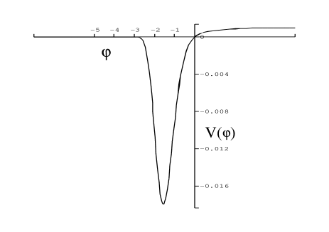
Figure 1: Typical cyclic potential [corresponding to parameters $V_{0}=10^{-3},m_{1}=0.2$ and $m_{2}=20/21$ in Eq. (14)].

In the 5-dimensional frame, the density and curvature on the visible brane remain finite at collision ekcyc . However, the fifth dimension itself degenerates at collision, and there is no well-posed Cauchy problem. The scale factor vanishes at collision, but the matter and radiation densities do not diverge at the instant of collision, owing to the coupling of $\varphi$ with matter and radiation. This evades the usual 4-dimensional singularity, but the problem re-appears as a singularity in the extra dimension. The key issue for the cyclic scenario is to find a 5-dimensional way through the collision, so as to be able to predict the cosmological perturbation spectra.

Our aim here is different. We are interested in the possible role of non-perturbative quantum corrections as the branes approach, i.e., near the steep minimum in the potential. To this end, we investigate how 4-dimensional loop quantum effects will alter the effective 4-dimensional dynamics of the cyclic scenario (since there is no 5-dimensional non-perturbative formalism).

The key point is that the steep negative potential produces a strong kinetic regime for the moduli field, and so we expect strong loop quantum corrections to be triggered. Previous results suggest that these corrections will prevent the singularity, i.e., the branes will come close but not actually collide. Essentially we confirm this expectation. However, we also find that it is difficult to achieve the bounce without passing from the semi-classical regime to the high-energy fully quantum regime, where our use of the effective 4-dimensional theory breaks down. The problem is that the kinetic energy and the Hubble rate typically reach Planckian scale as the branes approach, and then we have no handle on the dynamics and are unable to make predictions.

In the semi-classical regime where we can apply the loop corrections, brane collision is prevented. We cannot make predictions for the subsequent evolution since we neglect the radiation on the brane. Our results only apply in the near-brane regime where the moduli field is dominant.

II Dynamics in loop cosmology

The main modification in the classical general relativistic equations implied by loop quantum cosmology is that inverse powers of the scale factor in the matter Hamiltonian are replaced by a bounded function InvScale ; icgc . This can be interpreted as a curvature cut-off naturally following from the discrete structure underlying the loop quantization. For a scalar field the Hamiltonian is

$${\cal H}=\frac{1}{2}d(a)p_{\varphi}^{2}+a^{3}V(\varphi)\,,$$ (1)

where $p_{\varphi}$ is the momentum canonically conjugate to $\varphi$, and $d(a)$, which is classically $1/a^{3}$, encodes the quantum corrections. In the semi-classical regime, where spacetime may be treated as continuous, it is given by

$$d(a)={D(q)\over a^{3}}\,,~{}q={a^{2}\over a_{*}^{2}}\,,~{}a_{*}=\sqrt{{\gamma j\over 3}}\,\ell_{\rm Pl}\,.$$ (2)

where $j$ (a half integer) is a quantization parameter, $\gamma\approx 0.13$ is the Barbero-Immirzi parameter, $\ell_{\rm Pl}$ is the Planck length and

$$D(q)=q^{-3/2}\left\{\frac{3}{2l}\left({1\over l+2}\left[(q+1)^{l+2}-|q-1|^{l+2}\right]\right.\right.$$

$$-\left.\left.\frac{q}{1+l}\left[(q+1)^{l+1}-{\rm sgn}(q-1)|q-1|^{l+1}\right]\right)\right\}^{3/(2-2l)}\!.$$ (3)

Here $l$ is another quantization parameter, with $0<l<1$. This expression for $D(q)$ was derived in InvScale for $l=3/4$ as an approximation to the eigenvalues of inverse scale factor operators in loop quantum cosmology, and generalized in icgc to arbitrary $0<l<1$. The approximation to the eigenvalues becomes better for values of $j$ larger than the minimal one, $1/2$.

The scale below which non-perturbative modifications become important is given by $a_{*}$. Typically, one chooses $j\gg 1$, so that $a_{*}\gg\ell_{\rm Pl}$. The Planck scale marks the onset of discrete spacetime effects. For $\ell_{\rm Pl}<a\ll a_{*}$, we are in the semi-classical non-perturbative regime, where the geometrical density behaves as

$$d(a)\sim\left[\left({3\over 1+l}\right)^{3/(2-2l)}\left({a\over a_{*}}\right)^{3(2-l)/(1-l)}\right]{1\over a^{3}}\,.$$ (4)

The Hamiltonian determines the dynamics completely. The matter Hamiltonian leads to the Klein-Gordon equation via the Hamiltonian equations of motion. This first equation gives

$$\dot{\varphi}=\{\varphi,{\cal H}\}=d(a)p_{\varphi}\,.$$ (5)

The second Hamiltonian equation of motion for $p_{\varphi}$ can then be recast into a second order equation for $\varphi$ inf_martin ; inf_cmb ; bounce_closed ,

$$\ddot{\varphi}+\left(3H-\frac{\dot{D}}{D}\right)\dot{\varphi}+D\,V_{,\varphi}=0\,.$$ (6)

For $\ell_{\rm Pl}<a\ll a_{*}$, we find that $\dot{D}/D>3H$, and this leads to the classical frictional term for an expanding universe becoming anti-frictional, or vice versa if the universe is contracting.

The Friedman equation follows by equating the matter Hamiltonian and the gravitational contribution $3\dot{a}^{2}a$,

$$H^{2}=\frac{8\pi G}{3}\left[\frac{\dot{\varphi}^{2}}{2D(a)}+V(\varphi)\right]\,.$$ (7)

Finally, the Raychaudhuri equation follows from a Hamiltonian equation of motion for the gravitational Hamiltonian constraint:

$$\frac{\ddot{a}}{a}=-\frac{8\pi G}{3}\left[\frac{\dot{\varphi}^{2}}{D}\,\left(1-\frac{\dot{D}}{4HD}\right)-V(\varphi)\right]\,.$$ (8)

The Friedman equation implies that a bounce in the scale factor, i.e., $\dot{a}=0$ and $\ddot{a}>0$, requires a negative potential. (In a closed model, the curvature term allows for a bounce with positive potential bounce_closed .) This occurs for a negative cosmological constant or the potential considered in cyclic models. Vanishing Hubble parameter at the bounce implies

$$\dot{\varphi}^{2}={-2D(a)V(\varphi)}\,,$$ (9)

so that at the bounce,

$$\frac{\ddot{a}}{a}=\frac{4\pi G}{3}\left(6-\frac{{\mathrm{d}}\ln D}{{\mathrm{d}}\ln a}\right)V\,.$$ (10)

Thus classically, i.e., for $D=1$, a bounce for a negative $V(\varphi)$ is not allowed. With the modified $D(a)$, however, ${\mathrm{d}}\ln D/{\mathrm{d}}\ln a>6$ will hold for sufficiently small $a$, so that $\ddot{a}>0$ is possible. Thus, the universe has to collapse sufficiently deep into the modified regime before it can bounce back. In this regime, $D(a)$ is decreasing with shrinking scale factor, so that $\dot{\varphi}^{2}$ around the bounce, given by Eq. (9), is very small. Thus the scalar field almost freezes, which can also be seen as a consequence of the loop quantum friction effect in the Klein-Gordon equation for a contracting universe. In general relativity, the corresponding term is strongly anti-frictional during collapse, so that $\dot{\varphi}^{2}$ increases and no turn-around is possible.

After the bounce, $\varphi$ unfreezes and continues its motion with $|\dot{\varphi}|$ becoming larger. Another consequence of the Friedman equation with a negative scalar potential, is that $\dot{\varphi}$ cannot become exactly zero, so that $\varphi$ will not turn around and just slow down during the bounce. The bounce in scale factor is not a bounce in $\varphi$. Some time after the bounce, the universe may recollapse, which also is possible only for a negative potential. In contrast to the bounce, however, this is a purely classical effect, since the volume has become large.

III Loop quantum effects for a cyclic potential

We start with a simple illustration for the case of constant negative potential (or a negative cosmological constant), which will be followed by a typical potential used in the cyclic scenario.

III.1 Negative cosmological constant

For a free massless scalar field in a constant negative potential $V=\Lambda/8\pi G\equiv\lambda$, the Klein-Gordon equation (6) can be integrated once to obtain $\dot{\varphi}=CD(a)/a^{3}$, where $C$ is a constant. Inserting this into the Friedman equation (7) gives

$$\dot{a}^{2}-\frac{8\pi G}{3}\left[C^{2}\frac{D(a)}{2a^{4}}+\lambda a^{2}\right]=0\,.$$ (11)

The evolution of the scale factor is determined by the effective potential

$$V_{\rm eff}=-\frac{C^{2}}{2}\frac{D(a)}{a^{4}}-\lambda a^{2}\,.$$ (12)

This potential already demonstrates the difference between the classical and the loop quantum cases. Classically, the first term dominates at small $a$, so that $V_{\rm eff}\to-\infty$. Thus $a\to 0$ and a singularity follows. With the quantum modified $D(a)$, however, the potential approaches zero at $a=0$, and there is a barrier of positive potential at small $a$. At intermediate $a$, extending from the modified region to large $a$, there is a classically allowed region which describes the periodic motion of the scalar. At large $a$ there is a turning point in both the classical and the effective case.

Since the maximal scale factor $a_{\rm max}$ lies in the classical regime, we have $D(a_{\rm max})\approx 1$ at $V_{\rm eff}(a_{\rm max})=0$, so that $a_{\rm max}\approx(-C^{2}/2\lambda)^{1/6}$. The minimum scale factor $a_{\rm min}$ lies in the modified regime. For $(\ell_{\rm Pl}<)a_{\rm min}\ll a_{*}$, we can use Eq. (4) to obtain $D(a_{\rm min})\approx Ba^{3(2-l)/(1-l)}$, where $B\equiv[3/(1+l)]^{3/(2-2l)}$. By Eq. (12), $a_{\rm min}\approx(-2\lambda/BC^{2})^{(1-l)/3l}$. Thus, the cosmological constant must be small enough, $|\lambda|<C^{2}B^{(2-2l)/(2-l)}/2$ for a consistent solution, i.e., $a_{\rm min}<a_{\rm max}$.

The equations of motion can be solved in this case up to integrations. From Eq. (11) we obtain $t(a)=\int{\mathrm{d}}a[-V_{\rm eff}(a)]^{-1/2}$, which upon inversion leads to $a(t)$ so that $\dot{\varphi}=CD(a)/a^{3}$ can be integrated. The resulting motion for $a$ is periodic, while $\varphi$ changes monotonically (with periodic $\dot{\varphi}$). The period is given by

$$T = 2\int_{a_{\rm min}}^{a_{\rm max}}\frac{{\mathrm{d}}a}{\dot{a}}$$ (13)

$$= \sqrt{3}\int_{a_{\rm min}}^{a_{\rm max}}\frac{{\mathrm{d}}a}{\sqrt{\pi G(C^{2}a^{-4}D(a)-2|\lambda|a^{2})}}\,.$$

III.2 Cyclic potential

When the potential is negative but non-constant, the scale factor still behaves cyclically, but non-periodically. The size of the scale factor at recollapse changes between cycles in a way depending on the potential. This case is in particular relevant for cyclic models which consider the potential (see Fig. 1)

$$V(\varphi)=V_{0}\,(1-e^{-\varphi/m_{1}})\exp(-e^{-\varphi/m_{2}})\,,$$ (14)

where $m_{i}$ are two energy scales, and we are using Planck units. This models an inter-brane attractive potential for the moduli field $\varphi$, which describes the brane separation via $e^{\varphi}$, so that the branes collide for $\varphi\to-\infty$. At the same time, the scale factor approaches zero following the classical equations of motion. However, the matter and radiation densities on the brane do not diverge.

This scenario critically relies on unknown and non-classical dynamics which occurs when branes collide and then re-emerge to move apart. Non-perturbative quantum corrections are needed to resolve this issue, but no suitable 5-dimensional formalism is available. Instead, one can try to apply the 4-dimensional loop quantum formalism as a non-perturbative correction to the effective 4-dimensional theory of the cyclic scenario.

We now have a detailed prescription for quantum gravity effects in the semi-classical regime which modify the scalar field dynamics describing this situation. Before $\varphi$ reaches $-\infty$, the scale factor enters the regime where the frictional term in the modified Klein-Gordon equation slows down the scalar $\varphi$ while $a$ bounces back. Subsequently, $\varphi$ does not turn around but continues to decrease. The comparative evolution of the scale factor, moduli field and Hubble rate, with and without loop quantum effects, is illustrated in Figs. 2–4. The classical cyclic universe has $a\to 0$ in a finite time, whereas for the same set of parameters but with loop quantum corrections, the universe bounces back before a singularity occurs. In the standard cyclic scenario, as $\varphi$ runs down the steep negative potential, the Hubble parameter exceeds the Planck energy in the 4-dimensional frame, but this can be avoided via loop quantum corrections if the initial scale factor at the onset of collapse is small enough rn (see the solid curve in Fig. 4 compared to the classical dashed curve).

Since the potential is not constant, the behavior of expansion and recollapse of the scale factor will not be periodic but will still be cyclic. The constant potential indicates that the smaller the magnitude of the potential, the larger the expansion between a bounce and the following recollapse, which is also suggested by the figures. However, we are unable to draw definite conclusions about the behaviour after the first avoidance of collision, since we have neglected the matter and radiation on the visible brane, so that we cannot predict the late-time expansion and subsequent recollapse. From the quantum modification in the near-brane regime where $\varphi$ dominates, it follows that the bounce is non-singular and the singularity is removed. Note that there is a series of bounces at finite values of $\varphi$, and due to the slowing down of $\varphi$ during bounces, the moduli field does not reach $-\infty$ as in the standard case (see the solid curve in Fig. 3). In this sense $\varphi\to-\infty$ is not a singularity but rather a boundary at infinity.

Figure 2: The evolution of the scale factor $a(t)$ from a small initial value, for the cyclic potential. The dashed curve shows the standard case, while the solid curve incorporates loop quantum corrections, which stop the branes from colliding. The loop parameters are $j=120$ and $l=3/4$ and the cyclic parameters are $V_{0}=10^{-3}$, $m_{1}=0.2$, $m_{2}=20/21$.

Figure 3: Evolution of the moduli field $\varphi(t)$ for the case described in Fig. 2.

Figure 4: Evolution of the Hubble rate $H(t)$ for the case described in Fig. 2.

IV Conclusions

The problem of unknown dynamics near brane collisions has been a constraint on developments for the cyclic scenario. It is expected that quantum gravity will resolve this issue, but no fully non-perturbative higher-dimensional formalism has been available for tackling this problem. In the absence of such a formalism, we have applied loop quantum gravity to find non-perturbative corrections (in the semi-classical regime, $\ell_{\rm Pl}<a\ll a_{*}$) to the effective 4-dimensional theory of the cyclic scenario, using a typical potential. These non-perturbative corrections lead to very different dynamics compared to the standard classical effective dynamics.

We have considered the regime where branes are close to each other and the moduli field is dominant over matter and radiation, which we have neglected. As the branes approach each other and the moduli field runs down the steep negative potential, the kinetic term becomes dominant and the loop quantum effects freeze the field. Classically, in the 4-dimensional frame the cyclic universe would have gone into a big crunch with the Hubble parameter rapidly becoming much bigger than Planck energy (in the 5-dimensional frame this corresponds to brane collision with no singularity on the branes ekcyc ). However, the loop quantum gravity effects avoid the big crunch. The Hubble parameter can be kept below the Planck energy by choosing the initial scale factor small enough. If the scale factor is much larger than $a_{*}$ at the instant when collapse starts, then the Hubble parameter will violate the Planck bound, and we cannot apply the semi-classical equations used here, since spacetime becomes discretized. This is an unavoidable restriction for the potential considered, and shows that fully quantum gravity dynamics are needed to study the general problem. However, our limited results suggest that avoidance of brane collision may be a general feature. Moreover, since in the cases studied here the bounce value of the scale factor lies well above the Planck regime, we can trust the effective semi-classical equations used throughout, and do not have to refer to a more complicated analysis in terms of wave functions.

It would be interesting to see whether further input from string/ M theory leads to similar conclusions. This would introduce new ingredients via the intrinsic properties of branes as quantum objects. In order to make a more meaningful comparison however, it would be necessary to go beyond the 4-dimensional approach used here, and derive a 5-dimensional loop quantum gravity scheme for the full bulk spacetime. The spatial inhomogeneity of the bulk represents a considerable challenge to this project. But the importance of the project goes beyond the cyclic scenario – a higher-dimensional loop quantum gravity formalism may provide the basis for useful interaction between this approach and the string theory approach to quantum gravity.

Acknowledgements: We thank Jim Lidsey, David Mulryne, Nelson Nunes and Reza Tavakol for helpful discussions. RM’s work is supported by PPARC. PS thanks Max-Planck-Institut für Gravitationsphysik, Portsmouth University and Queen Mary, University of London for supporting visits and for warm hospitality during various stages of this work.

References

- (1) J. Khoury et al., Phys. Rev. D 64, 123522 (2001) [arXiv:hep-th/0103239]; P. J. Steinhardt & N. Turok, arXiv:hep-th/0111030; Phys. Rev. D 65, 126003 (2002) [arXiv:hep-th/0111098]; J. Khoury, P. J. Steinhardt & N. Turok, Phys. Rev. Lett. 92, 031302 (2004) [arXiv:hep-th/0307132].
- (2) C. Rovelli, Liv. Rev. Rel. 1, 1 (1998) [arXiv:gr-qc/9710008]; T. Thiemann, Lect. Notes Phys. 631, 41 (2003) [arXiv:gr-qc/0210094]; A. Ashtekar and J. Lewandowski, Class. Quant. Grav. 21, R53 (2004) [arXiv:gr-qc/0404018].
- (3) C. Rovelli & L. Smolin, Nucl. Phys. B 442, 593 (1995) [arXiv:gr-qc/9411005]; A. Ashtekar & J. Lewandowski, Class. Quant. Grav. 14, A55 (1997) [arXiv:gr-qc/9602046]; T. Thiemann, J. Math. Phys. 39, 3347 (1998) [arXiv:gr-qc/9606091].
- (4) T. Thiemann, Class. Quant. Grav. 15, 1281 (1998) [arXiv:gr-qc/9705019].
- (5) K. Krasnov, Gen. Rel. Grav. 30, 53 (1998) [arXiv:gr-qc/9605047]; C. Rovelli, Phys. Rev. Lett. 77, 3288 (1996) [arXix:gr-qc/9603063]; A. Ashtekar, J. Baez, A. Corichi & K. Krasnov, Phys. Rev. Lett. 80, 904 (1998) [arXiv:gr-qc/9710007].
- (6) M. Bojowald & H. A. Morales-Técotl, Lect. Notes Phys. 646, 421 (2004) [arXiv:gr-qc/0306008].
- (7) M. Bojowald, Pramana (in press) [arXiv:gr-qc/0402053].
- (8) M. Bojowald, Phys. Rev. Lett. 86, 5227 (2001) [arXiv:gr-qc/0102069]; M. Bojowald, Class. Quant. Grav. 19, 2717 (2002) [arXiv:gr-qc/0202077]; A. Ashtekar, M. Bojowald & J. Lewandowski, Adv. Theor. Math. Phys. 7, 233 (2003) [arXiv:gr-qc/0304074]; M. Bojowald, Class. Quant. Grav. 20, 2595 (2003); M. Bojowald, G. Date & K. Vandersloot, Class. Quant. Grav. 21, 1253 (2004) [arXiv:gr-qc/0311004].
- (9) M. Bojowald, Phys. Rev. Lett. 87, 121301 (2001) [arXiv:gr-qc/0104072]; M. Bojowald, Gen. Rel. Grav. 35, 1877 (2003) [arXiv:gr-qc/0305069]; D. Cartin, G. Khanna and M. Bojowald, Class. Quant. Grav. 21, 4495 (2004) [arXiv:gr-qc/0405126].
- (10) M. Bojowald, Class. Quant. Grav. 18, L109 (2001) [arXiv:gr-qc/0105113].
- (11) M. Bojowald, P. Singh and A. Skirzewski, gr-qc/0408094.
- (12) M. Bojowald, Phys. Rev. D 64, 084018 (2001) [arXiv:gr-qc/0105067]; M. Bojowald, Class. Quant. Grav. 19, 5113 (2002) [arXiv:gr-qc/0206053].
- (13) M. Bojowald, Phys. Rev. Lett. 89, 261301 (2002) [arXiv:gr-qc/0206054]; M. Bojowald & K. Vandersloot, Phys. Rev. D 67, 124023 (2003) [arXiv:gr-qc/0303072].
- (14) S. Tsujikawa, P. Singh & R. Maartens, arXiv:astro-ph/0311015.
- (15) M. Bojowald et al., Phys. Rev. D 70, 043530 (2004) [arXiv:gr-qc/0403106].
- (16) P. Singh & A. Toporensky, Phys. Rev. D 69, 104008 (2004) [arXiv:gr-qc/0312110]; G. V. Vereshchagin, JCAP 0407, 013 (2004) [arXiv:gr-qc/0406108].
- (17) J. Lidsey, D. Mulryne, N. Nunes, R. Tavakol, Phys. Rev. D 70, 063521 (2004) [arXiv: gr-qc/0406042].
- (18) M. Bojowald & G. Date, Phys. Rev. Lett. 92, 071302 (2004) [arXiv:gr-qc/0311003]; M. Bojowald, G. Date & G. Hossain, Class. Quant. Grav. 21, 3541 (2004) [arXiv:gr-qc/0404039].
- (19) This was pointed out to us by J. Lidsey, D. Mulryne, N. Nunes and R. Tavakol.