hep-th/0407101

AEI-2004-040

DAMTP 2004-52

$E_{10}$ and $SO(9,9)$ invariant supergravity
A. Kleinschmidt
Department of Applied Mathematics and Theoretical Physics
Centre for Mathematical Sciences, Wilberforce Road, Cambridge CB3 0WA, U.K.
a.kleinschmidt@damtp.cam.ac.uk

H. Nicolai
Max-Planck-Institut für Gravitationsphysik
Mühlenberg 1, D-14476 Golm, Germany
nicolai@aei.mpg.de

We show that (massive) $D=10$ type IIA supergravity possesses a hidden rigid $D_{9}\equiv SO(9,9)$ symmetry and a hidden local $SO(9)\times SO(9)$ symmetry upon dimensional reduction to one (time-like) dimension. We explicitly construct the associated locally supersymmetric Lagrangian in one dimension, and show that its bosonic sector, including the mass term, can be equivalently described by a truncation of an $E_{10}/K(E_{10})$ non-linear ${\sigma}$-model to the level $\ell\leq 2$ sector in a decomposition of $E_{10}$ under its $D_{9}$ subalgebra. This decomposition is presented up to level $\ell=10$, and the even and odd level sectors are identified tentatively with the Neveu–Schwarz and Ramond sectors, respectively. Further truncation to the level $\ell=0$ sector yields a model related to the reduction of $D=10$ type I supergravity. The hyperbolic Kac–Moody algebra $DE_{10}$, associated to the latter, is shown to be a proper subalgebra of $E_{10}$, in accord with the embedding of type I into type IIA supergravity. The corresponding decomposition of $DE_{10}$ under $D_{9}$ is presented up to level $\ell=5$.

1 Introduction

Dimensional reduction of supergravity theories has proved to be not only a way of constructing lower dimensional theories with extended supersymmetry, but also a way of revealing hidden symmetries [1, 2]. The example studied most thoroughly in this context is that of maximal eleven dimensional supergravity [3], which upon dimensional reduction gives rise to the chain of exceptional hidden symmetries $E_{n(n)}$. Below three uncompactified dimensions, the relevant Kac–Moody algebras are infinite dimensional [4].

In one dimension, the expected hidden symmetry is the elusive hyperbolic $E_{10}$ symmetry whose root space geometry is known to govern the behavior of cosmological solutions of $D=11$ supergravity near a space-like singularity [5, 6, 7]. These so-called cosmological billiards were also studied in the context of other over-extended Kac–Moody algebras, see [8, 9, 10, 11, 12]. In the toroidal compactification of $D=11$ supergravity to one time dimension there is a manifest $GL(10;{\mathbb{R}})$ symmetry acting on the internal components. By making use of a ‘level expansion’ of $E_{10}$ in terms of $GL(10;{\mathbb{R}})$ tensors, it was shown in [13] that the equations of motion of a ${\sigma}$-model on the $E_{10}/K(E_{10})$ coset space, when truncated to the first three levels, are equivalent to a restricted version of the bosonic equations of motion of $D=11$ supergravity where only the fields and their first order spatial gradients at a given spatial point are retained. It was furthermore shown there that the level decomposition of $E_{10}$ contains representations that can be naturally associated to the spatial gradients of the bosonic $D=11$ supergravity fields. This observation gave rise to the conjecture that the geodesic motion on the $E_{10}/K(E_{10})$ coset manifold can capture the full space-time dependence of the $D=11$ supergravity fields, such that the standard BKL approximation is recovered via a ‘small tension expansion’ in spatial gradients. However, the $E_{10}$ $\sigma$-model is expected to contain many further degrees of freedom, because the representations corresponding to spatial gradients constitute only a tiny subset of the $E_{10}$ Lie algebra [14].

The aim of the present paper is two-fold. First, we demonstrate that (massive) type IIA supergravity [15] reduced to one time-like dimension admits a hidden symmetry $SO(9,9)/SO(9)\times SO(9)$. The same symmetry appears already for the reduction of type I supergravity to one dimension, which is obtained from the IIA theory by restricting to the Neveu–Schwarz type fields. These results extend earlier ones on the emergence of $SO(n,n)$ symmetries in dimensionally reduced type I supergravity [16, 17, 18]. The hidden $SO(9,9)$ symmetry group has a natural interpretation in string theory, being the continuous T-duality group of the low energy effective action of the two type II string theories reduced to one dimension, whose discrete subgroup $SO(9,9;{\mathbb{Z}})$ is known to be a good quantum symmetry of the perturbative string spectrum [19, 20].

The second main result of this paper is an analysis of the $E_{10}/K(E_{10})$ coset model at low levels in terms of a level decomposition of $E_{10}$ under its $D_{9}\equiv SO(9,9)$ subgroup, complementing the results of [13] where a level decomposition of $E_{10}$ w.r.t. its $A_{9}\equiv SL(10;{\mathbb{R}})$ subgroup was used. Just like $SL(10,{\mathbb{R}})$, the group $SO(9,9)$ is a regular subgroup of $E_{10}$, and its maximal compact subgroup $SO(9)\times SO(9)$ is a subgroup of $K(E_{10})$, the maximal compact subgroup of $E_{10}$. Accordingly, we now decompose $E_{10}$ into an infinite tower of $SO(9,9)$ representations, with the level as the ‘floor number’. We then proceed to use this decomposition to compare the dynamics of the truncated ${\sigma}$-model to the reduced bosonic equations of motion.

In comparison with [13], the present results reveal several new facets. In particular, the decomposition of $E_{10}$ into $SO(9,9)$ assigns a special role to the $10$-th spatial dimension. The compact $SO(9)\times SO(9)$ subgroup has as its diagonal subgroup $SO(9)_{\rm diag\,}$, which is the remnant of the Lorentz group acting on nine compact spatial dimensions only. The last coordinate direction corresponds to a dilatonic field ${\varphi}$ (not the standard IIA dilaton), which is orthogonal to $SO(9,9)$ and algebraically provides the desired grading of $E_{10}$ w.r.t. its $D_{9}$ subalgebra. Another new feature is the appearance of spinorial representations of $SO(9,9)$ at odd levels in the level decomposition: while the vectorial representations corresponding to the Neveu–Schwarz-Neveu–Schwarz (NSNS) fields appear at even levels, the Ramond-Ramond (RR) type fields are associated with the odd levels. Our terminology here is loose in the sense that we refer to any state composed as a product of two vectorial representations of $SO(9)$ as an NSNS field, and to any state composed out of two spinorial representations of $SO(9)$ as an RR field. Restricting to the even level NSNS sector, one obtains the non-maximal type I theory which is simpler to study in the present context. Its reduction to one dimension likewise admits a $SO(9,9)/SO(9)\times SO(9)$ invariant formulation. In the corresponding $E_{10}$ model, the type I theory corresponds to level $\ell=0$ in the decomposition which forms a closed subalgebra of ${\mathfrak{e}}_{10}$. Because $SO(9,9)$ is also contained in $DE_{10}$, which has been conjectured to be a hidden symmetry of type I supergravity reduced to one dimension [4, 5], analogous statements hold true for the coset $DE_{10}/K(DE_{10})$. The mutual consistency of these conjectures is a consequence of the fact that $DE_{10}$ is generated by a proper (irregular) subalgebra of ${\mathfrak{e}}_{10}$. When extending these results to type IIA supergravity we have to embed RR fields into representations of $SO(9,9)$, which we are able to do by adding their duals and a Romans mass term (which in the present context is best understood in terms of a 9-form [15, 23, 24, 25]). This is in precise agreement with the structure found at $\ell=1$ in the decomposition of $E_{10}$ under its $D_{9}$ subalgebra, and shows that massive IIA supergravity, too, can be accommodated within $E_{10}$.

Unlike previous work, our analysis also includes the fermionic degrees of freedom, albeit only ‘at level $\ell=0$’. In particular, we demonstrate that the fermions can also be placed into multiplets of $SO(9)\times SO(9)$ in this approach. Furthermore, we determine the relevant $\sigma$-model quantities from the supersymmetry variations; the bosonic equations of motion, which were used for this purpose in [13], then provide an additional and independent consistency check. While the supersymmetry algebra in the type I case closes on shell on the finite set of fields obtained by reduction of type I supergravity, it acquires new terms in the type II case, which no longer close on the finite set of fields obtained by $SO(9)\times SO(9)$ ‘covariantization’ of the type II supergravity fields. The necessity of (in fact, infinitely many) new fields follows algebraically by noting that, unlike the level 0 representations, the level $\ell=-1,0,1$ representations do not form a subalgebra of ${\mathfrak{e}}_{10}$, but instead generate all of the ${\mathfrak{e}}_{10}$ algebra. However, it must be stressed that even the most basic aspects of the fermionic sector in relation to the hyperbolic symmetry remain to be understood. Whereas it is known at least in principle how to recursively construct the additional bosonic degrees of freedom in the $E_{10}$ model (cf. the tables of [14] and appendices B and C of this paper), it remains an outstanding challenge to also extend the fermionic $SO(9)\times SO(9)$ multiplets to a full spinor (i.e. double valued) representation of $K(E_{10})$, and to write down a locally supersymmetric model compatible with local $K(E_{10})$ symmetry.

A non-linear realization of massive IIA supergravity [26], and the embedding of the bosonic sector of type I into that of type II supergravity [27] were already investigated in the context of an earlier, and conceptually different, proposal concerning the realization of hidden Kac–Moody symmetries in M-theory [28, 29, 30, 31] (see also [32, 33, 34]). According to that proposal, $D=11$ supergravity admits an M-theoretic extension possessing an even larger symmetry containing a hidden $E_{11}$, which is also supposed to accommodate type IIB supergravity [34]. The indefinite Kac–Moody algebra $E_{11}$ is not hyperbolic any more, but belongs to a class of Lorentzian Kac–Moody algebras called very extended algebras [35]. In a related development, the Weyl group of $E_{11}$ was shown to act on the moduli of Kasner solutions [36] and to generate the intersection rules for branes [37]. A $\sigma$-model approach, which aims to merge the proposals of [13] and [28] by introducing an unphysical auxiliary parameter, was recently formulated and studied in [38, 39].

For $E_{10}$, a ‘brany’ interpretation of the imaginary roots has been proposed in [40]; furthermore, these authors conjecture that essential information about M-theory compactified on $T^{10}$ is contained in a generalized modular form over the coset space $E_{10}({\mathbb{Z}})\!\setminus\!E_{10}/K(E_{10})$. This modular form can be viewed as the solution of the Wheeler–DeWitt equation that is (formally) obtained by quantizing the Hamiltonian constraint of [13]. Very similar ideas have been put forth in [41]. Finally, an attempt to merge M(atrix) theory and $E_{11}$ has been made in [42].

The paper is organized as follows. We first explain our conventions and notations in section 2. In section 3 the $SO(9,9)$ invariance of reduced type I and type IIA supergravity is studied indicating the necessity of introducing additional fields to obtain an $SO(9,9)$ invariant, locally supersymmetric theory in the latter case. This could be provided for by studying the $E_{10}$ model and we carry out the required decomposition in section 4. These results are then exploited in section 5 to give the equations of motion of the truncated ${\sigma}$-model based on $E_{10}$ where the resulting dynamics are linked to the reduced supergravities from section 3. In appendix A, we fix our choice of gamma matrices. Appendices B and C contain the details of the decomposition of $E_{10}$ and $DE_{10}$ with respect to their regular $D_{9}$ subalgebras. This decompositions are presented up to levels $\ell=10$ for $E_{10}$ and $\ell=5$ for $DE_{10}$ in this paper.

2 Conventions

The action of $D=11$, $N=1$ supergravity to second order in fermions [3] in our conventions is

$$S = \int d^{11}xE\left(-\frac{1}{4\kappa_{11}^{2}}R-\frac{i}{2}\bar{\Psi}_{M}\Gamma^{MNP}\nabla_{N}\Psi_{P}-\frac{1}{48}F_{MNPQ}F^{MNPQ}\right){}$$

$$-\frac{i\kappa_{11}}{96}\int d^{11}xE\left(\bar{\Psi}_{M}{\Gamma}^{MNPQRS}\Psi_{S}+12\bar{\Psi}^{N}{\Gamma}^{PQ}\Psi^{R}\right)F_{NPQR}$$

$$+\frac{2\kappa_{11}}{(144)^{2}}\int d^{11}x{\epsilon}^{M_{1}\ldots M_{11}}F_{M_{1}\ldots M_{4}}F_{M_{5}\ldots M_{8}}A_{M_{9}\ldots M_{11}}+\ldots.{}$$

We will set Newton’s constant to $\kappa_{11}=1$. The ellipsis denotes additional couplings and higher order Fermi terms which will not be of relevance in our analysis. The above action is invariant under the supersymmetry variations [3]

$${\delta}{E_{M}}^{A} = i\bar{\epsilon}{\Gamma}^{A}\Psi_{M},$$ (2.2a)

$${\delta}A_{MNP} = \frac{3}{2}i\bar{\epsilon}{\Gamma}_{[MN}\Psi_{P]},$$ (2.2b)

$${\delta}\Psi_{M} = \left(\partial_{M}{\epsilon}+\frac{1}{4}\omega_{M\,AB}{\Gamma}^{AB}{\epsilon}\right)-\frac{1}{144}\big{(}{{\Gamma}_{M}}^{NPQR}-8{\delta}_{M}^{N}{\Gamma}^{PQR}\big{)}{\epsilon}F_{NPQR},$$ (2.2c)

where we have only kept terms up to linear order in fermions in the variation of the fermions.

From (2) we deduce the bosonic equations of motions

$$\partial_{M}\big{(}EF^{MNPQ}\big{)} = -\frac{1}{576}E{\epsilon}^{NPQR_{1}\ldots R_{4}S_{1}\ldots S_{4}}F_{R_{1}\ldots R_{4}}F_{S_{1}\ldots S_{4}},$$ (2.3a)

$$R_{MN} = -\frac{1}{3}F_{MP_{1}P_{2}P_{3}}F_{N}{}^{P_{1}P_{2}P_{3}}+\frac{1}{36}G_{MN}F_{P_{1}P_{2}P_{3}P_{4}}F^{P_{1}P_{2}P_{3}P_{4}}.$$ (2.3b)

In addition we have the Bianchi identity

$$\partial_{[M}F_{NPQR]}=0.$$ (2.4)

Let us also fix our notations for the reduction from eleven to one dimension at this point. We perform a $(1+9+1)$ split of the coordinates and label the coordinates of the three different sectors according to the following list:

$$\begin{array}[]{rclll}M,N,...&=&t,\tilde{1},...,{\widetilde{10}}&&\mbox{curved indices in $D=11$}\\ A,B,...&=&0,1,...,10&&\mbox{flat indices in $D=11$}\\ {\hat{m}},{\hat{n}},...&=&\tilde{1},...,{\widetilde{10}}&&\mbox{curved spatial indices in $D=11$}\\ {\hat{a}},{\hat{b}},...&=&1,...,10&&\mbox{flat spatial indices in $D=11$}\\ m,n,...&=&\tilde{1},...,\tilde{9}&&\mbox{curved spatial indices in $D=10$}\\ a,b,...&=&1,...,9&&\mbox{flat spatial indices in $D=10$}\end{array}{}$$ (2.11)

To distinguish flat indices from curved ones, we will put a tilde on the latter, e.g. ${\widetilde{10}}$. Below, we will furthermore need indices pertaining to the $SO(9,9)/SO(9)\times SO(9)$ coset space; these are

$$\begin{array}[]{rclll}I,J,...&\in&\{1,...,18\}&&\mbox{for $SO(9,9)$}\\ i,j,...&\in&\{1,...,9\}&&\mbox{for the first $SO(9)$}\\ {\bar{\imath}},{\bar{\jmath}\,},...&\in&\{\bar{1},...,\bar{9}\}\equiv\{10,...,18\}&&\mbox{for the second $SO(9)$}\\ {\alpha},{\beta},...&\in&\{1,...,16\}&&\mbox{spinor indices for the first $SO(9)$}\\ {\bar{\alpha}},{\bar{\beta}},...&\in&\{1,...,16\}&&\mbox{spinor indices for the second $SO(9)$}\end{array}{}$$ (2.17)

Finally, in later sections, we will also use indices $A,B,...$ for the 256-dimensional chiral spinor representations of $SO(9,9)$ and ${\dot{A}},{\dot{B}},...$ for the conjugate spinor. Our ${\gamma}$-matrix conventions for the orthogonal groups $SO(9)$, $SO(1,10)$ and $SO(9,9)$ are listed in the separate appendix A.

3 $SO(9,9)$ invariant supergravity in one dimension

In this section we study the dimensional reduction of (2) to one timelike dimension, but in a setting that is appropriate to IIA supergravity, and the $SO(9,9)$ symmetry which we wish to exhibit. To this end we perform a (9+1) split of the ten spatial coordinates taking us through $D=10$ supergravity. We first study the type I theory and find that it can be written as a coset model on the space $SO(9,9)/SO(9)\times SO(9)$ with additional dilaton. Extending the analysis to type IIA supergravity the additional fields generate new terms both in the Lagrangian and the supersymmetry variations and a locally supersymmetric version as a coset model is no longer possible with a finite dimensional coset space.

We first consider the reduction of the elfbein degrees of freedom in the $(1+9+1)$ split of the coordinates. Keeping an arbitrary lapse function $N$ and setting the shift variables to zero, the elfbein of $D=11$ supergravity reads

$${E_{M}}^{A}=\left(\begin{array}[]{cc}N&0\\ 0&{\hat{E}_{\hat{m}}}{}^{{\hat{a}}}\end{array}\right)\quad\Longrightarrow\quad G_{MN}=\left(\begin{array}[]{cc}-N^{2}&0\\ 0&\hat{G}_{{\hat{m}}{\hat{n}}}\end{array}\right).$$ (3.5)

$N$ is a Lagrange multiplier enforcing reparametrisation invariance w.r.t. to the diffeomorphisms generated by timelike vector fields. Next we perform a (9+1) split of the spatial part of the elfbein in triangular gauge:

$${\hat{E}_{\hat{m}}}{}^{{\hat{a}}}=\left(\begin{array}[]{cc}{E_{m}}^{a}&e^{\frac{1}{2}\phi}A_{m}\\ 0&e^{\frac{1}{2}\phi}\end{array}\right)\quad\Longrightarrow\quad{\hat{E}_{\hat{a}}}{}^{{\hat{m}}}=\left(\begin{array}[]{cc}{E_{a}}^{m}&-{E_{a}}^{m}A_{m}\\ 0&e^{-\frac{1}{2}\phi}\end{array}\right).$$ (3.10)

The spatial metric and its inverse are given by

$$\hat{G}_{{\hat{m}}{\hat{n}}}=\left(\begin{array}[]{cc}G_{mn}+e^{\phi}A_{m}A_{n}&e^{\phi}A_{m}\\ e^{\phi}A_{n}&e^{\phi}\end{array}\right)\quad\Longrightarrow\quad\hat{G}^{{\hat{m}}{\hat{n}}}=\left(\begin{array}[]{cc}G^{mn}&-A^{m}\\ -A^{n}&e^{-\phi}+A^{r}A_{r}\end{array}\right).$$ (3.15)

Here, the index on $A^{m}$ has been raised with $G^{mn}$. In order to end up with a Lagrangian that has the required symmetries, we must still redefine the metric $G_{mn}$ and the dilaton $\phi$. The properly redefined fields $g_{mn}$ and ${\varphi}$ of the reduced theory are

$$e^{\varphi}=G^{-\frac{1}{2}}e^{-\frac{3}{4}\phi}\quad,\qquad{e_{m}}^{a}=e^{\frac{1}{4}\phi}{E_{m}}^{a}\quad\Longrightarrow\quad g_{mn}=e^{\frac{1}{2}\phi}G_{mn}.$$ (3.16)

By $G$ and $g$, we denote the determinants of $G_{mn}$ and $g_{mn}$, respectively; thus $g=e^{\frac{9}{2}\phi}G$. Inverting these relations, we obtain

$$G_{mn}=g^{\frac{1}{6}}e^{-\frac{1}{3}{\varphi}}g_{mn}\quad,\qquad e^{\phi}=g^{\frac{1}{3}}e^{\frac{2}{3}{\varphi}}.$$ (3.17)

While the field $\phi$ thus is just the standard dilaton, our ‘dilaton’ ${\varphi}$ differs from it by its additional dependence on the 9-metric $g_{mn}$. For this reason, ${\varphi}$ will appear in the Lagrangian in a way different from the way in which $\phi$ appears in the standard type I and type IIA Lagrangians.

A short calculation now shows that the reduction of Einstein’s action to one dimension indeed becomes diagonal in terms of the fields $g$, ${\varphi}$ and $A_{m}$, viz.

$$\hat{G}^{{\hat{m}}{\hat{n}}}{\partial_{t}}{\hat{G}}_{{\hat{n}}{\hat{p}}}\hat{G}^{{\hat{p}}{\hat{q}}}{\partial_{t}}{\hat{G}}_{\hat{\hat{q}}{\hat{m}}}-\left(\hat{G}^{{\hat{m}}{\hat{n}}}{\partial_{t}}{\hat{G}}_{{\hat{m}}{\hat{n}}}\right)^{2} = g^{mn}{\partial_{t}}{g}_{np}g^{pq}{\partial_{t}}{g}_{qn}-4{\partial_{t}}{\varphi}{\partial_{t}}{\varphi}{}$$ (3.18)

$$+2e^{{\varphi}}g^{\frac{1}{2}}g^{mn}{\partial_{t}}{A}_{m}{\partial_{t}}{A}_{n}.$$

Next, we turn to reduction of the eleven dimensional gravitino $\Psi_{M}$. Its temporal component $\Psi_{t}$, with 32 real spinor components, is a Lagrange multiplier field (enforcing the supersymmetry constraint), while its spatial components constitute a vector spinor of $SO(10)$ with a total of $10\times 32=320$ real components, corresponding to the $\bf{32}$ and $\bf{288}$ representations of $SO(10)$. A 32-component Majorana spinor in eleven dimensions reduces to two 16-component real spinors of $SO(9)$, while the vector part reduces to a vector plus a scalar. The subscript $t$ is to indicate the transformation properties of $\Psi_{t}$ under reparametrizations of the time coordinate $t$; the corresponding ‘flat’ object is $\Psi_{0}=N^{-1}\Psi_{t}$. With this split of the coordinates we introduce redefined fermion fields as

$${\tilde{\Psi}}_{t} = {\hat{G}}^{-\frac{1}{4}}\Big{(}\Psi_{t}-{\Gamma}_{t}{\Gamma}^{a}\Psi_{a}-{\Gamma}_{t}{\Gamma}^{10}\Psi_{10}\Big{)},$$ (3.19a)

$${\tilde{\Psi}}_{a} = {\hat{G}}^{\frac{1}{4}}\Big{(}\Psi_{a}+\frac{1}{2}{\Gamma}_{a}{\Gamma}^{10}\Psi_{10}\Big{)},$$ (3.19b)

$${\tilde{\Psi}}_{10} = {\hat{G}}^{\frac{1}{4}}\Big{(}-\frac{3}{2}\Psi_{10}-{\Gamma}_{10}{\Gamma}^{a}\Psi_{a}\Big{)},$$ (3.19c)

with ${\hat{G}}=\det{\hat{G}}_{{\hat{m}}{\hat{n}}}=Ge^{\phi}$. Inverting these formula, we obtain

$$\Psi_{t} = {\hat{G}}^{\frac{1}{4}}{\tilde{\Psi}}_{t}-\frac{1}{6}{\hat{G}}^{-\frac{1}{4}}{\Gamma}_{t}{\Gamma}^{a}{\tilde{\Psi}}_{a}-\frac{7}{6}{\hat{G}}^{-\frac{1}{4}}{\Gamma}_{t}{\Gamma}^{10}{\tilde{\Psi}}_{10},$$ (3.20a)

$$\Psi_{a} = {\hat{G}}^{-\frac{1}{4}}\Big{(}{\tilde{\Psi}}_{a}-\frac{1}{6}{\Gamma}_{a}{\Gamma}^{b}{\tilde{\Psi}}_{b}-\frac{1}{6}{\Gamma}_{a}{\Gamma}^{10}{\tilde{\Psi}}_{10}\Big{)},$$ (3.20b)

$$\Psi_{10} = {\hat{G}}^{-\frac{1}{4}}\Big{(}\frac{1}{3}{\tilde{\Psi}}_{10}+\frac{1}{3}{\Gamma}_{10}{\Gamma}^{a}{\tilde{\Psi}}_{a}\Big{)}.$$ (3.20c)

With the above redefinitions one can check that the derivative part of the fermion kinetic term reduces as

$$-\frac{i}{2}N{\sqrt{\hat{G}}}\bar{\Psi}_{A}{\Gamma}^{ABC}\partial_{B}\Psi_{C}=\frac{i}{2}{\tilde{\Psi}}_{a}^{T}{\partial_{t}}{\tilde{\Psi}}_{a}-\frac{i}{2}{\tilde{\Psi}}_{10}^{T}{\partial_{t}}{\tilde{\Psi}}_{10},$$ (3.21)

where we have used that $\bar{\Psi}=\Psi^{T}{\Gamma}^{0}$ in our conventions. The connection terms (of type $\omega\Psi^{2}$) in the kinetic term will be shown below to combine with the $F\Psi^{2}$ terms in (2) to give an $SO(9)\times SO(9)$-covariantization of the derivative above.

In the supersymmetry variations, the above redefinitions must be accompanied by the following rescaling of the supersymmetry transformation parameter with the opposite power of ${\hat{G}}$

$${\epsilon}\longrightarrow\varepsilon\equiv{\hat{G}}^{-1/4}{\epsilon}.$$ (3.22)

It is noteworthy that the redefinitions of the fermionic variables are the ones that one would expect on account of the corresponding formulae in higher dimensions; for instance, the general formula for the redefinitions of the gravitino field and the supersymmetry transformations parameter in Kaluza–Klein supergravity read

$$\psi^{\prime}_{\mu}={\hat{G}}^{\frac{1}{4}\frac{1}{2-d}}{e^{\prime}_{\mu}}^{\alpha}\big{(}\Psi_{\alpha}+\frac{1}{d-2}\Gamma_{\alpha}\Gamma^{a}\Psi_{a}\big{)}\quad,\qquad\varepsilon^{\prime}={\hat{G}}^{-\frac{1}{4}\frac{1}{2-d}}\varepsilon$$ (3.23)

where $\alpha$ and $a$ label the (flat) uncompactified and compactified coordinates, respectively, $d$ is the number of uncompactified dimensions, and ${\hat{G}}$ the determinant of the compactified part of the metric. Although these formulae obviously fail for $d=2$ they do work again for $d=1$!

3.1 Type I theory

We first restrict to the case of type I supergravity and show that it can be written with local $SO(9)\times SO(9)$ invariance in both the bosonic and the fermionic sector.

The bosonic fields of this theory are the zehnbein, an antisymmetric 2-form field and a dilaton, referred to as Neveu–Schwarz-Neveu–Schwarz fields in IIA string theory. Therefore we set the Kaluza–Klein vector of the metric $A_{m}=0$ in this section. The 2-form field of type I supergravity originates from the 3-form field $A_{MNP}$ in eleven dimensions, with $P={\widetilde{10}}$; all other components of the 3-form will be set to zero for the type I theory. The corresponding terms are most conveniently derived by first writing the relevant term in eleven dimensions with flat indices, and then reconverting to curved indices by means of the appropriate rescaled vielbeine. For the field $b_{mn}=2A_{mn{\widetilde{10}}}$ and adopting the Coulomb gauge $A_{tmn}=0$, this procedure yields for the kinetic term

$$\frac{1}{12}N{\sqrt{\hat{G}}}{\hat{G}}^{tt}G^{{\hat{m}}{\hat{q}}}G^{{\hat{n}}\hat{r}}G^{{\hat{p}}\hat{s}}F_{t\,{\hat{m}}{\hat{n}}{\hat{p}}}F_{t\,{\hat{q}}\hat{r}\hat{s}} \rightarrow$$

$$-\frac{1}{4}N^{-1}{\sqrt{\hat{G}}}{\hat{G}}^{mp}{\hat{G}}^{nq}{\hat{G}}^{\tilde{10}\tilde{10}}F_{t\,mn\tilde{10}}F_{t\,pq\tilde{10}} = -\frac{1}{16}N^{-1}\sqrt{\hat{G}}g^{mp}g^{nq}{\partial_{t}}b_{mn}{\partial_{t}}b_{pq};$$ (3.24)

note that the dilaton factor in the inverse metric prefactors cancels by virtue of our redefinition (3.16). Combining this with the result for the reduced Einstein action (3.18) the reduced action for the type I theory therefore reads

$$\frac{1}{16}\int dt\,N^{-1}{\sqrt{\hat{G}}}\left(g^{mn}{\partial_{t}}{g}_{np}g^{pq}{\partial_{t}}{g}_{qm}-g^{mn}{\partial_{t}}{b}_{np}g^{pq}{\partial_{t}}{b}_{qm}-4{\partial_{t}}{\varphi}{\partial_{t}}{\varphi}\right).$$ (3.25)

In string frame the type I bosonic Lagrangian comes with a dilatonic prefactor [43]. Here, however, we do not want such a factor, because we wish to embed this Lagrangian into an $E_{10}/K(E_{10})$ ${\sigma}$-model such that the level $\ell$ terms appear with a factor $e^{\ell{\varphi}}$, and therefore there should be no dilatonic prefactor for $\ell=0$ Lagrangian, corresponding to type I. For this reason we redefine the lapse according to

$$N=\sqrt{\hat{G}}\cdot n$$ (3.26)

with the new lapse function $n(t)$ (the gauge used in the cosmological billiard description [7] is then $n=1$). The supersymmetry partner of the latter is the redefined gravitino

$${\tilde{\Psi}}_{t}\equiv N{\tilde{\Psi}}_{0}=n{\hat{G}}^{\frac{1}{4}}\Big{(}\Psi_{0}-{\Gamma}_{0}{\Gamma}^{a}\Psi_{a}-{\Gamma}_{0}{\Gamma}^{10}\Psi_{10}\Big{)}$$ (3.27)

The bosonic type I Lagrangian (3.25) possesses a hidden $SO(9,9)$ symmetry which we can exhibit explicitly by parametrising the fields $g$ and $b$ in terms of a representative of the coset space ${\cal E}\in SO(9,9)/SO(9)\times SO(9)$

$${\cal E}(t)=\frac{1}{2}\left(\begin{array}[]{cc}1&1\\ -1&1\end{array}\right)\left(\begin{array}[]{cc}e^{-1}&-e^{-1}b\\ 0&e^{T}\end{array}\right)\left(\begin{array}[]{cc}1&-1\\ 1&1\end{array}\right)$$ (3.34)

in self-explanatory matrix notation (the calculation is analogous to the one in [17]). Because there are now two $SO(9)$ groups, we will use unbarred and barred $SO(9)$ indices $i,j,...$ and ${\bar{\imath}},{\bar{\jmath}\,},...$, respectively, to distinguish them; the previous $SO(9)$ indices $a,b,...$ then refer to the diagonal subgroup of $SO(9)\times SO(9)$. The metric $g_{mn}=e_{m}{}^{a}e_{n}{}^{a}$ can be read off from

$${\cal E}^{T}{\cal E}=\frac{1}{2}\left(\begin{array}[]{cc}1&1\\ -1&1\end{array}\right)\left(\begin{array}[]{cc}g^{-1}&-g^{-1}b\\ bg^{-1}&g-bg^{-1}b\end{array}\right)\left(\begin{array}[]{cc}1&-1\\ 1&1\end{array}\right).$$ (3.41)

To write down the Lagrangian, we need

$${\partial_{t}}{\cal E}{\cal E}^{-1}={\textstyle{\frac{1}{2}}}Q^{ij}X_{ij}+{\textstyle{\frac{1}{2}}}Q_{{\bar{\imath}}{\bar{\jmath}\,}}X^{{\bar{\imath}}{\bar{\jmath}\,}}+P_{i{\bar{\jmath}\,}}Y^{i{\bar{\jmath}\,}}.$$ (3.42)

where $(Q_{ij},Q_{{\bar{\imath}}{\bar{\jmath}\,}})$ is the gauge field for the compact $SO(9)\times SO(9)$ subgroup. The Lie algebra elements $X^{ij}$ and $X^{{\bar{\imath}}{\bar{\jmath}\,}}$ are the generators of the compact $SO(9)\times SO(9)$ subgroup and the $Y^{i{\bar{\jmath}\,}}$ are the remaining (broken) generators of the full $SO(9,9)$. The explicit expressions are

$$Q_{ij} = {e_{[i}}^{m}{\partial_{t}}e_{mj]}+\frac{1}{2}{e_{i}}^{m}{e_{j}}^{n}{\partial_{t}}b_{mn},$$ (3.43a)

$$Q_{{\bar{\imath}}{\bar{\jmath}\,}} = {e_{[i}}^{m}{\partial_{t}}e_{mj]}-\frac{1}{2}{e_{i}}^{m}{e_{j}}^{n}{\partial_{t}}b_{mn},$$ (3.43b)

$$P_{i{\bar{\jmath}\,}} = {e_{(i}}^{m}{\partial_{t}}e_{mj)}-\frac{1}{2}{e_{i}}^{m}{e_{j}}^{n}{\partial_{t}}b_{mn}.$$ (3.43c)

Not forgetting the dilaton, which transforms as a singlet under $SO(9,9)$, and whose kinetic term appears with a minus sign, the bosonic Lagrangian from equation (3.25) can be written as

$${\cal L}_{I}=\frac{1}{4}n^{-1}\big{(}P_{i{\bar{\jmath}\,}}P_{i{\bar{\jmath}\,}}-{\partial_{t}}{\varphi}{\partial_{t}}{\varphi}\big{)}$$ (3.44)

where $n$ is a lapse function already introduced above.

To exhibit the $SO(9)\times SO(9)$ invariance of the fermionic sector, we regroup the 320 gravitino components into irreducible multiplets of $SO(9)\times SO(9)$. Because a 32-component Majorana spinor in $D=11$ reduces to two 16-component $D=10$ spinors and a $D=10$ vector reduces to a $D=9$ vector and a scalar, we split the spatial components of the $D=11$ gravitino as follows:

$$\begin{array}[]{ccccccccc}{\bf 320}\rightarrow&({\bf 9},{\bf 16})&+&({\bf 1},{\bf 16})&+&({\bf 16},{\bf 9})&+&({\bf 16},{\bf 1})\\ &\chi_{i{\bar{\alpha}}}&&\chi_{{\bar{\alpha}}}&&\chi_{{\bar{\imath}}{\alpha}}&&\chi_{{\alpha}}\end{array}$$ (3.47)

The essential point here is that the vector and spinor indices are now decreed to transform under two different $SO(9)$ groups as indicated by the replacement of $a$ by $i$ and ${\bar{\imath}}$, respectively, and the split of $SO(1,10)$ spinor indices into ${\alpha}$ and ${\bar{\alpha}}$. The consistency of these assignments does not follow from dimensional reduction alone, but must instead be verified by direct computation. The kinetic term for the fermions from equation (3.21) can be written as

$$\frac{i}{2}\tilde{\Psi}_{a}^{T}\partial_{t}\tilde{\Psi}_{a}-\frac{i}{2}\tilde{\Psi}^{T}\partial_{t}\tilde{\Psi}=\frac{i}{2}\chi_{i{\bar{\alpha}}}{\partial_{t}}\chi_{i{\bar{\alpha}}}+\frac{i}{2}\chi_{{\bar{\imath}}{\alpha}}{\partial_{t}}\chi_{{\bar{\imath}}{\alpha}}-\frac{i}{2}\chi_{\alpha}{\partial_{t}}\chi_{\alpha}-\frac{i}{2}\chi_{\bar{\alpha}}{\partial_{t}}\chi_{\bar{\alpha}},$$ (3.48)

exhibiting global $SO(9)\times SO(9)$ invariance . The derivative terms in (3.48) combine with the contributions from the spin connection and $F\Psi^{2}$ terms in the $D=11$ supergravity theory in such a way as to give a covariantization of the derivative under local $SO(9)\times SO(9)$ transformations. As we are considering the type I theory in this section, we retain only one chiral half of the fermions, say $\chi_{\alpha}$ and $\chi_{{\bar{\jmath}\,}{\alpha}}$, from (3.48).

The supersymmetry transformations (2.2) determine the transformations of the reduced fields which we also need to re-express in our new set of variables. From the variation (2.2a) in $D=11$ we obtain

$${E_{(a}}^{m}{\delta}E_{mb)}=i\bar{\epsilon}{\Gamma}_{(a}\Psi_{b)}\quad,\qquad{\delta}\phi=2i\bar{\epsilon}{\Gamma}^{10}\Psi_{10}.$$ (3.49)

For the first relation a compensating $SO(10)$ rotation for maintaining the triangular gauge of the zehnbein $\hat{E}_{\hat{m}}{}^{\hat{a}}$ was necessary. Together with the redefinitions from eq. (3.16), (3.19) and (3.22) this yields

$${e_{(a}}^{m}{\delta}e_{mb)}=i\bar{\varepsilon}{\Gamma}_{(a}\tilde{\Psi}_{b)}\quad,\qquad{\delta}{\varphi}=-i\bar{\varepsilon}{\Gamma}_{10}\tilde{\Psi}_{10}.$$ (3.50)

For the Lagrange multiplier $n=N\hat{G}^{-1/2}$, an analogous calculation leads to the simple result

$${\delta}n=-i\varepsilon_{\alpha}\psi_{t{\alpha}}.$$ (3.51)

For the variation of the three form field $A_{mn{\widetilde{10}}}$, we similarly obtain

$${\delta}A_{mn{\widetilde{10}}}=\frac{1}{2}{\delta}b_{mn}=\frac{1}{2}i\bar{\epsilon}{\Gamma}_{mn}\Psi_{{\widetilde{10}}}+i\bar{\epsilon}{\Gamma}_{{\widetilde{10}}}{\Gamma}_{[m}\Psi_{n]}=i\bar{\varepsilon}{\Gamma}_{{\widetilde{10}}}{\Gamma}_{[m}\tilde{\Psi}_{n]}$$ (3.52)

Because the matrix ${\Gamma}_{10}$ separates the two $SO(9)$’s (cf. appendix A.2), we can cast these variations into an $SO(9)\times SO(9)$ covariant form by means of the redefined fermions and supersymmetry parameters (of course, retaining only one chiral half of (3.47)) and obtain

$${e_{(i}}^{m}{\delta}e_{mj)}-\frac{1}{2}{e_{i}}^{m}{e_{j}}^{n}\,{\delta}b_{mn}=i\varepsilon_{\alpha}{\gamma}_{i{\alpha}{\beta}}\chi_{{\bar{\jmath}\,}{\beta}}\equiv\Lambda_{i{\bar{\jmath}\,}},$$ (3.53a)

$${\delta}{\varphi}=i{\epsilon}_{\alpha}\chi_{\alpha}.$$ (3.53b)

The variations of the metric $g_{mn}$ and the NS 2-form can thus be recast into a manifestly $SO(9)\times SO(9)$ covariant form

$${\delta}{\cal E}{\cal E}^{-1}=\Lambda_{i{\bar{\jmath}\,}}Y^{i{\bar{\jmath}\,}}.$$ (3.54)

whence

$${\delta}P_{i{\bar{\jmath}\,}} = D_{t}\Lambda_{i{\bar{\jmath}\,}}\equiv{\partial_{t}}\Lambda_{i{\bar{\jmath}\,}}+Q_{ik}\Lambda_{k{\bar{\jmath}\,}}+Q_{{\bar{\jmath}\,}{\bar{k}}}\Lambda_{i{\bar{k}}},$$ (3.55a)

$${\delta}Q_{ij} = -2\Lambda_{[i|{\bar{k}}|}P_{j]{\bar{k}}}\quad,\qquad{\delta}Q_{{\bar{\imath}}{\bar{\jmath}\,}}=-2\Lambda_{k[{\bar{\imath}}}P_{|k|{\bar{\jmath}\,}]}.$$ (3.55b)

where $D_{t}$ is a $SO(9)\times SO(9)$ covariant derivative.

The variations of the fermions can be likewise determined from eq. (2.2c), making use of all the redefinitions introduced above. Again, one finds (after some computation) that all formulae can be cast into a manifestly $SO(9)\times SO(9)$ covariant form. Because the calculation is completely analogous to the one for the bosonic fields, we refrain from presenting further details here, but simply collect the pertinent formulae in (3.59) below.

In summa, we obtain the following Lagrangian for type I reduced to one dimension with local $SO(9)\times SO(9)$ invariance

$${\cal L}_{{\rm I}} = \frac{1}{4}n^{-1}\big{(}P_{i{\bar{\jmath}\,}}P_{i{\bar{\jmath}\,}}-\dot{\varphi}^{2}\big{)}-\frac{i}{2}\chi_{\alpha}D_{t}\chi_{\alpha}+\frac{i}{2}\chi_{{\bar{\jmath}\,}{\alpha}}D_{t}\chi_{{\bar{\jmath}\,}{\alpha}}{}$$ (3.56)

$$+\frac{i}{2}n^{-1}\psi_{t{\alpha}}\chi_{\alpha}{\dot{\varphi}}-\frac{i}{2}n^{-1}\psi_{t{\alpha}}{\gamma}_{i{\alpha}{\beta}}\chi_{{\bar{\jmath}\,}{\beta}}P_{i{\bar{\jmath}\,}}+\ldots$$

modulo higher order fermionic corrections. The derivatives on the fermions are $SO(9)\times SO(9)$ covariant, for instance

$$D_{t}\chi_{{\bar{\imath}}{\alpha}}=\partial_{t}\chi_{{\bar{\imath}}{\alpha}}+{\textstyle{\frac{1}{4}}}Q_{jk}{\gamma}^{jk}_{{\alpha}{\beta}}\chi_{{\bar{\imath}}{\beta}}+Q_{{\bar{\imath}}{\bar{\jmath}\,}}\chi_{{\bar{\jmath}\,}{\alpha}}.$$ (3.57)

The supersymmetry variations, which leave ${\cal L}_{{\rm I}}$ invariant, are, for the bosonic fields,

$${\delta}P_{i{\bar{\jmath}\,}} = D_{t}(i\varepsilon{\gamma}_{i}\chi_{{\bar{\jmath}\,}}),$$ (3.58a)

$${\delta}{\varphi} = i\varepsilon\chi,$$ (3.58b)

$${\delta}n = -i\varepsilon\psi_{t}.$$ (3.58c)

The fermionic variations, with the cubic corrections needed for the closure of the supersymmetry algebra below, read

$${\delta}\psi_{t{\alpha}} = D_{t}\varepsilon_{\alpha}-\frac{i}{4}n({\gamma}_{ij}\varepsilon)_{\alpha}\,\chi{\gamma}_{ij}\chi+\frac{i}{4}n({\gamma}_{ij}\varepsilon)_{\alpha}\,\chi_{{\bar{k}}}{\gamma}_{ij}\chi_{{\bar{k}}},$$ (3.59a)

$${\delta}\chi_{\alpha} = -\frac{1}{2}n^{-1}\varepsilon_{\alpha}(\dot{\varphi}-i\psi_{t}\chi),$$ (3.59b)

$${\delta}\chi_{{\bar{\jmath}\,}{\alpha}} = -\frac{1}{2}n^{-1}({\gamma}_{i}\varepsilon)_{\alpha}(P_{i{\bar{\jmath}\,}}-i\psi_{t}{\gamma}_{i}\chi_{{\bar{\jmath}\,}}).$$ (3.59c)

Modulo the fermionic equations of motion, the supersymmetry algebra closes and is $SO(9)\times SO(9)$ covariant on all fields

$$[{\delta}_{1},{\delta}_{2}]n =\partial_{t}(\xi^{t}n), [{\delta}_{1},{\delta}_{2}]\psi_{t{\alpha}} =0,{}$$

$${}[{\delta}_{1},{\delta}_{2}]\varphi =\xi^{t}\partial_{t}{\varphi}+{\delta}_{\varepsilon^{\prime}}{\varphi}, [\delta_{1},\delta_{2}]\chi_{\alpha} =0,$$ (3.60)

$${}[{\delta}_{1},{\delta}_{2}]P_{i{\bar{\jmath}\,}} =\partial_{t}(\xi^{t}P_{i{\bar{\jmath}\,}})+{\delta}_{\varepsilon^{\prime}}P_{i{\bar{\jmath}\,}}+{\delta}_{\omega}P_{i{\bar{\jmath}\,}}, [\delta_{1},\delta_{2}]\chi_{{\bar{\jmath}\,}{\alpha}} =0,{}$$

where $\xi^{t}:=-in^{-1}\varepsilon_{2{\alpha}}\varepsilon_{1{\alpha}}$ is the standard (time) translation parameter, $\varepsilon^{\prime}_{\alpha}=-\xi^{t}\psi_{t{\alpha}}$ a new local supersymmetry transformation parameter, and $\omega$ an $SO(9)\times SO(9)$ transformation with parameters

$$\omega_{ij} = \xi^{t}Q_{ij}-2\chi_{\bar{k}}{\gamma}_{i}\varepsilon_{[1}\,\varepsilon_{2]}{\gamma}_{j}\chi_{\bar{k}},$$ (3.61a)

$$\omega_{{\bar{\imath}}{\bar{\jmath}\,}} = \xi^{t}Q_{{\bar{\imath}}{\bar{\jmath}\,}}-2\chi_{k}{\gamma}_{{\bar{\imath}}}\varepsilon_{[1}\,\varepsilon_{2]}{\gamma}_{{\bar{\jmath}\,}]}\chi_{k}.$$ (3.61b)

This is precisely the form of the standard supersymmetry algebra in theories of supergravity (in an on-shell formulation such as ours): the commutator of two supersymmetry transformations yields a translation term with parameter $\xi^{\mu}=i\varepsilon_{1}{\gamma}^{\mu}\varepsilon_{2}$, a local supersymmetry transformation with parameter $\varepsilon^{\prime}=-\xi^{\mu}\psi_{\mu}$ (see e.g. [46], section 1.9) and a local gauge transformation, here in the form of a local $SO(9)\times SO(9)$ transformation with parameters $(\omega_{ij},\omega_{{\bar{\imath}}{\bar{\jmath}\,}})$. The on-shell vanishing of the algebra (3.1) on the fermion fields is a consequence of this general structure in the reduction to one dimension. For example, on the Lagrange multiplier $\psi_{t}$, the contributions cancel by virtue of

$$D_{t}{\epsilon}^{\prime}_{\alpha}+D_{t}(\xi^{t}\psi_{t{\alpha}})=0.$$ (3.62)

The closure on the matter fermions $\chi$ and $\chi_{\bar{\jmath}\,}$ requires in addition the fermionic field equations

$$D_{t}\chi_{\alpha}+\frac{1}{2}n^{-1}\psi_{t{\alpha}}\dot{\varphi} = 0,$$ (3.63a)

$$D_{t}\chi_{{\bar{\jmath}\,}{\alpha}}+\frac{1}{2}({\gamma}_{i}\psi_{t})_{\alpha}P_{i{\bar{\jmath}\,}} = 0.$$ (3.63b)

3.2 Type IIA theory

To extend type I to type IIA supergravity, we must complement the type I fermions by those of the opposite chirality, and incorporate the Kaluza–Klein vector $A_{m}$ together with the remaining components of the 3-form field in eleven dimensions, namely $A_{mnp}$. In string theory both arise from the Ramond-Ramond (RR) sector; for this reason we will refer to them as RR type fields. With the Coulomb (temporal) gauge $A_{t}=A_{tmn}=0$, the time derivatives of the RR fields coincide with the field strengths of the unreduced theory

$$F_{tmnp}\equiv{\partial_{t}}A_{mnp}=\frac{1}{2}{\partial_{t}}a_{mnp}\quad;\qquad F_{tm}\equiv{\partial_{t}}a_{m}.$$ (3.64)

Repeating the calculation leading to (3.1), the combined contribution of the Kaluza–Klein vector $a_{m}\equiv A_{m}$ from (3.18) and of $a_{mnp}\equiv 2A_{mnp}$ is thus equal to

$$\frac{1}{4}n^{-1}e^{{\varphi}}g^{\frac{1}{2}}\left(\frac{1}{2}\cdot\frac{1}{3!}g^{mq}g^{nr}g^{ps}{\partial_{t}}a_{mnp}{\partial_{t}}a_{qrs}+\frac{1}{2}g^{mn}{\partial_{t}}a_{m}{\partial_{t}}a_{n}\right),$$ (3.65)

Observe that the dilaton prefactor in (3.65) is the same for the 3-form and the Kaluza Klein vector, and is indeed the desired prefactor for level $\ell=1$. In addition, there is a common factor of ${\sqrt{g}}$, which will turn out to be precisely what is required for the $\sigma$-model (and can be viewed as originating from a ‘spinorial metric’ acting on the odd level fields). As anticipated, our dilaton ${\varphi}$ (defined by Eq. (3.16)) couples in a way different from the standard type IIA dilaton: in string frame, the latter does not appear in front of the RR kinetic terms [43].

The RR form potentials thus give rise to the $SO(9)$ tensors $a^{(p)}$ for $p=1$ and $p=3$. By themselves, these fields are not enough to allow for the larger symmetry $SO(9)\times SO(9)$ or global $SO(9,9)$. However, we can enhance the symmetry group in the desired way by adding forms of degree $p=5,7$ and $9$. Namely, these fields can be then combined into a single irreducible spinor representation of $SO(9,9)$, which under the $SO(9)\times SO(9)$ subgroup becomes the $({\bf 16},{\bf 16})$ bispinor representation, and under the diagonal $SO(9)_{\rm diag\,}$ subgroup decomposes as

$$\bf{16}\otimes\bf{16}=\bf{1}\oplus\bf{9}\oplus\bf{36}\oplus\bf{84}\oplus{126}$$ (3.66)

At the linearized level, we thus assemble the RR degrees of freedom into

$$\phi_{{\alpha}{\bar{\alpha}}}\equiv\phi_{{\alpha}{\bar{\alpha}}}^{{\rm(IIA)}}=\sum_{p=1,3,5,7,9}\frac{1}{p!}\,{\gamma}^{a_{1}\ldots a_{p}}_{{\alpha}{\bar{\alpha}}}a_{a_{1}\ldots a_{p}}^{(p)}.$$ (3.67)

As we will see, this is precisely the structure arising at level $\ell=1$ in the decomposition of $E_{10}$ under its $SO(9,9)$ subgroup. Under the diagonal $SO(9)$ subgroup of $SO(9)\times SO(9)$ we thus recover the required representations for forms with odd $p$. The 5- and 7-forms will be interpreted as the dual RR forms, respectively, which in the reduced theory are associated to the first order spatial gradients of $a_{m}$ and $a_{mnp}$. The 9-form, on the other hand, does not appear in $D=11$ supergravity, but is associated with the Romans’ type mass term in the IIA theory [15, 23, 25]. In contrast to the $A_{9}$ decomposition of [13], where the fields and their duals appeared at different levels, the level $\ell=1$ sector thus contains both the RR type fields and their duals. By contrast, the dual degrees of freedom for the $\ell=0$ NSNS fields appear only at level $\ell=2$. The formula (3.67) also admits a type IIB interpretation: by means of the formulae of Appendix A.1 we can rewrite it as a sum over even $p$,

$$\phi_{{\alpha}{\bar{\alpha}}}^{{\rm(IIB)}}=\sum_{p=0,2,4,6,8}\frac{1}{p!}\,{\gamma}^{a_{1}\ldots a_{p}}_{{\alpha}{\bar{\alpha}}}{\tilde{a}}_{a_{1}\ldots a_{p}}^{(p)}.$$ (3.68)

This rewriting simply reflects the equivalence of the type IIA and IIB supergravity theories upon dimensional reduction.

In order to properly identify the RR degrees of freedom at the non-linear level, we adopt a procedure that differs from [13] in so far as we deduce the relevant expressions from the supersymmetry variations, and not by direct comparison with the (bosonic) equations of motion. Instead, the latter, which we will study in section 4, will provide us with an independent consistency check. Accordingly, we proceed from the following ansatz for the fermionic variations of the type II theory, encompassing the NSNS and RR degrees of freedom up to level $\ell=1$,

$${\delta}\psi_{t{\alpha}} = D_{t}\varepsilon_{\alpha}+e^{\frac{1}{2}{\varphi}}P_{{\alpha}{\bar{\alpha}}}\varepsilon_{\bar{\alpha}},$$ (3.69a)

$${\delta}\psi_{t{\bar{\alpha}}} = D_{t}\varepsilon_{\bar{\alpha}}-e^{\frac{1}{2}{\varphi}}\varepsilon_{\alpha}P_{{\alpha}{\bar{\alpha}}},$$ (3.69b)

$${\delta}\chi_{\alpha} = -\frac{1}{2}n^{-1}\dot{\varphi}\varepsilon_{\alpha}-\frac{1}{2}n^{-1}e^{\frac{1}{2}{\varphi}}P_{{\alpha}{\bar{\alpha}}}\varepsilon_{\bar{\alpha}},$$ (3.69c)

$${\delta}\chi_{\bar{\alpha}} = -\frac{1}{2}n^{-1}\dot{\varphi}\varepsilon_{\bar{\alpha}}+\frac{1}{2}n^{-1}e^{\frac{1}{2}{\varphi}}P_{{\alpha}{\bar{\alpha}}}\varepsilon_{\alpha},$$ (3.69d)

$${\delta}\chi_{i{\bar{\alpha}}} = -\frac{1}{2}n^{-1}P_{i{\bar{\jmath}\,}}{\gamma}_{{\bar{\jmath}\,}{\bar{\alpha}}{\bar{\beta}}}\varepsilon_{\bar{\beta}}-\frac{1}{2}n^{-1}\varepsilon_{\beta}{\gamma}_{i{\beta}{\alpha}}e^{\frac{1}{2}{\varphi}}P_{{\alpha}{\bar{\alpha}}},$$ (3.69e)

$${\delta}\chi_{{\bar{\jmath}\,}{\alpha}} = -\frac{1}{2}n^{-1}P_{i{\bar{\jmath}\,}}{\gamma}_{i{\alpha}{\beta}}\varepsilon_{\beta}+\frac{1}{2}n^{-1}\varepsilon_{\bar{\beta}}{\gamma}_{{\bar{\jmath}\,}{\bar{\beta}}{\bar{\alpha}}}e^{\frac{1}{2}{\varphi}}P_{{\alpha}{\bar{\alpha}}},$$ (3.69f)

where $P_{{\alpha}{\bar{\alpha}}}$ is the full nonlinear extension of the time derivative of the RR field $\phi_{{\alpha}{\bar{\alpha}}}$ in (3.67). (Below, we will separately discuss the level $\ell=2$ contributions to these variations, which correspond to the spatial gradients of the NSNS fields.) The terms involving NSNS degrees of freedom in (3.69) are simply obtained by ‘doubling’ the corresponding variations of the type I theory derived in the previous section. As for the RR type fields, consistency with local $SO(9)\times SO(9)$ invariance requires that they all appear via the single field strength $P_{{\alpha}{\bar{\alpha}}}$. For instance, the contributions from $F_{tmnp}$ to the variations of the redefined fermions are found to be (after some algebra, and using flat indices)

$${\delta}{\tilde{\Psi}}_{t} \ni \frac{1}{12}{\Gamma}^{abc}\varepsilon\,F_{tabc},$$ (3.70a)

$${\delta}{\tilde{\Psi}}_{a} \ni -\frac{1}{24}n^{-1}{\Gamma}^{bcd}{{\Gamma}_{a}}\varepsilon\,F_{tbcd},$$ (3.70b)

$${\delta}{\tilde{\Psi}}_{10} \ni \frac{1}{24}n^{-1}{\Gamma}_{10}{\Gamma}^{0}{\Gamma}^{bcd}\varepsilon\,F_{tbcd}.$$ (3.70c)

Rewriting this in terms of curved indices and the redefined neunbein and dilaton we obtain

$${\Gamma}^{abc}\varepsilon\,F_{tabc} = {\Gamma}^{abc}\varepsilon\,\big{(}{E_{a}}^{m}{E_{b}}^{n}{E_{c}}^{p}F_{tmnp}+3{E_{a}}^{m}{E_{b}}^{n}{E_{c}}^{\widetilde{10}}F_{tmn{\widetilde{10}}}\big{)}{}$$ (3.71)

$$= {\Gamma}^{abc}\varepsilon\,e^{\frac{3}{4}\phi}e_{a}{}^{m}e_{b}{}^{n}e_{c}{}^{p}G_{tmnp}={\Gamma}^{abc}\varepsilon\,e^{\frac{1}{2}{\varphi}}g^{\frac{1}{4}}e_{a}{}^{m}e_{b}{}^{n}e_{c}{}^{p}G_{tmnp}$$

with

$$G_{tmnp}:=F_{tmnp}-3A_{[m}F_{np]t{\widetilde{10}}}.$$ (3.72)

Comparing with (3.69) we can read off the corresponding contribution to $P_{{\alpha}{\bar{\alpha}}}$ and check that the field strength $G_{tmnp}$ (and hence also $F_{tmnp}$) indeed appears with the same coefficient in all variations.

The redefinition (3.72) is due to the reconversion from flat back to curved indices by means of the rescaled neunbeine ${e_{m}}^{a}$ from (3.16). Together with the analogous redefinition

$$G_{mnpq}:=F_{mnpq}+4A_{[m}F_{npq]{\widetilde{10}}},$$ (3.73)

it is well known from Kaluza Klein theory and ensures that these field strengths do not transform under reparametrizations of the 10-th spatial coordinate ${\delta}x^{{\widetilde{10}}}=\xi^{{\widetilde{10}}}(t)$. Note that the NSNS field strength $F_{tmn{\widetilde{10}}}$ and the Kaluza–Klein fields $F_{tm}$ and $F_{mn}$ do not receive any corrections of this form. The new field strengths obey the modified Bianchi identities (cf. (2.4))

$${\partial_{t}}G_{mnpq}-4\partial_{[m}G_{|t|npq]} = 4F_{t[m}F_{npq]{\widetilde{10}}}+6F_{[mn}F_{pq]t{\widetilde{10}}}{}$$ (3.74)

$$\qquad+4A_{[m}{\partial_{t}}F_{npq]{\widetilde{10}}}-12A_{[m}\partial_{n}F_{pq]t{\widetilde{10}}}$$

The remaining contributions from $F_{tm}$ and the (gauge invariant) spatial gradients $F_{mn}$ and $G_{mnpq}$ are worked out similarly. The Kaluza–Klein vector $A_{m}$ appears via the coefficients of anholonomity

$$\Omega_{0a\,10} = N^{-1}e^{\frac{3}{4}\phi}\cdot{e_{a}}^{m}F_{tm}$$ (3.75a)

$$\Omega_{ab\,10} = e^{\phi}\cdot{e_{a}}^{m}{e_{b}}^{n}F_{mn}$$ (3.75b)

Some further calculation then yields the final result

$$P_{{\alpha}{\bar{\alpha}}} = g^{\frac{1}{4}}\Bigg{[}ne^{-{\varphi}}M{\delta}_{{\alpha}{\bar{\alpha}}}+\frac{1}{4}{\gamma}^{m}_{{\alpha}{\bar{\alpha}}}F_{tm}+\frac{1}{8}{\gamma}^{mn}_{{\alpha}{\bar{\alpha}}}ne^{-{\varphi}}F_{mn}+{}$$ (3.76)

$$\qquad\qquad+\frac{1}{12}{\gamma}^{mnp}_{{\alpha}{\bar{\alpha}}}G_{tmnp}-\frac{1}{48}{\gamma}^{mnpq}_{{\alpha}{\bar{\alpha}}}ne^{-{\varphi}}G_{mnpq}\Bigg{]},$$

where we now and henceforth set ${\gamma}^{m}={\gamma}^{a}e_{a}{}^{m}$ etc., using the redefined neunbein fields (3.16). The (constant) $M$ corresponds to a Romans type mass term, which exists only for type IIA supergravity in ten dimensions, but vanishes for $D=11$ supergravity. Note also the prefactors of $ne^{-{\varphi}}$ in front of the terms containing even degree ${\gamma}$-matrices, i.e. spatial gradients.

Although (3.76) is the most convenient form to check against the equations of motion and Bianchi identities (see section 4), it is also straightforward to rewrite this expression in the form (3.67), dualizing the 4-, 2- and 0-forms into 5-, 7- and 9-forms by means of the formulae of the appendix. For instance, for the 4-form $G_{mnpq}$ we obtain (keeping track of the extra vielbein factor ${E_{\widetilde{10}}}^{10}$!)

$$G_{m_{1}\ldots m_{4}} = E_{m_{1}}{}^{a_{1}}\cdots E_{m_{4}}{}^{a_{4}}{\epsilon}_{a_{1}\ldots a_{4}}{}^{b_{1}\ldots b_{5}}N^{-1}E_{b_{1}}{}^{n_{1}}\cdots E_{b_{5}}{}^{n_{5}}e^{-\frac{1}{2}\phi}{\tilde{F}}_{tn_{1}\ldots n_{5}{\widetilde{10}}}{}$$ (3.77)

$$= N^{-1}e^{-\frac{1}{4}\phi}e_{m_{1}}{}^{a_{1}}\cdots e_{m_{4}}{}^{a_{4}}{\epsilon}_{a_{1}\ldots a_{4}}{}^{b_{1}\ldots b_{5}}e_{b_{1}}{}^{n_{1}}\cdots e_{b_{5}}{}^{n_{5}}{\tilde{F}}_{tn_{1}\ldots n_{5}{\widetilde{10}}}$$

or

$$G_{m_{1}\ldots m_{4}}=n^{-1}e^{\varphi}\cdot{e_{m_{1}}}^{a_{1}}\cdots{e_{m_{4}}}^{a_{4}}{\epsilon}_{a_{1}\ldots a_{4}}{}^{b_{1}\ldots b_{5}}e_{b_{1}}{}^{n_{1}}\cdots e_{b_{5}}{}^{n_{5}}{\tilde{F}}_{tn_{1}\ldots n_{5}{\widetilde{10}}}.$$ (3.78)

The prefactor $n^{-1}e^{\varphi}$ here conveniently cancels the dilaton dependence in front of $F_{mnpq}$ in (3.76). Similarly, when dualizing the exact Kaluza–Klein vector field strength by

$$e^{\phi}F_{mn}=E_{m}{}^{a}E_{n}{}^{b}{\epsilon}_{ab}{}^{c_{1}\ldots c_{7}}N^{-1}e^{-\frac{1}{2}\phi}E_{c_{1}}{}^{m_{1}}\cdots E_{c_{7}}{}^{m_{7}}{\tilde{F}}_{tm_{1}\ldots m_{7}{\widetilde{10}}},$$ (3.79)

we find

$$F_{mn} = N^{-1}e^{-\frac{1}{4}\phi}e_{m}{}^{a}e_{n}{}^{b}{\epsilon}_{ab}{}^{c_{1}\ldots c_{7}}e_{c_{1}}{}^{m_{1}}\cdots e_{c_{7}}{}^{m_{7}}{\tilde{F}}_{tm_{1}\ldots m_{7}{\widetilde{10}}}{}$$ (3.80)

$$= n^{-1}e^{\varphi}\cdot e_{m}{}^{a}e_{n}{}^{b}{\epsilon}_{ab}{}^{c_{1}\ldots c_{7}}e_{c_{1}}{}^{m_{1}}\cdots e_{c_{7}}{}^{m_{7}}{\tilde{F}}_{tm_{1}\ldots m_{7}{\widetilde{10}}}$$

again cancelling the prefactor in (3.76). An analogous calculation works for the prefactor of the Romans mass $M$ after dualization to a $9$-form. Hence, we can rewrite the expansion (3.76) in the form

$$P_{{\alpha}{\bar{\alpha}}} = g^{\frac{1}{4}}\Bigg{[}\frac{1}{4}{\gamma}^{m_{1}}_{{\alpha}{\bar{\alpha}}}F_{tm_{1}}+\frac{1}{12}{\gamma}^{m_{1}\ldots m_{3}}_{{\alpha}{\bar{\alpha}}}G_{tm_{1}\ldots m_{3}}-\frac{1}{48}{\gamma}^{m_{1}\ldots m_{5}}_{{\alpha}{\bar{\alpha}}}F_{tm_{1}\ldots m_{5}}{}$$ (3.81)

$$\qquad\qquad+\frac{1}{4\cdot 7!}{\gamma}^{m_{1}\ldots m_{7}}_{{\alpha}{\bar{\alpha}}}F_{tm_{1}\ldots m_{7}}+\frac{1}{9!}{\gamma}^{m_{1}\ldots m_{9}}_{{\alpha}{\bar{\alpha}}}F_{tm_{1}\ldots m_{9}}\Bigg{]},$$

where we have dropped additional ${\widetilde{10}}$ indices and tildes on the dual fields. This formula entails kinetic terms for the dual field strengths of the form

$$n^{-1}e^{\varphi}g^{m_{1}n_{1}}\cdots g^{m_{p}n_{p}}{F}_{tm_{1}\ldots m_{p}}F_{tn_{1}\ldots n_{p}},$$ (3.82)

for $p=5,7,9$ supplementing and generalizing the terms in (3.65).

After these preparations we are now ready to give the supersymmetry variations of the bosonic degrees of freedom, as well as the type II Lagrangian. The variation of the bosonic type I fields are again obtained by ‘doubling’ since we now have to include two sets of fermions, and read

$${\delta}n = -i(\varepsilon_{\alpha}\psi_{t{\alpha}}+\varepsilon_{\bar{\alpha}}\psi_{t{\bar{\alpha}}}),$$ (3.83a)

$${\delta}{\varphi} = i(\varepsilon_{\alpha}\chi_{\alpha}+\varepsilon_{\bar{\alpha}}\chi_{\bar{\alpha}}),$$ (3.83b)

$${\delta}P_{i{\bar{\jmath}\,}} = D_{t}(i\varepsilon_{\alpha}{\gamma}_{i{\alpha}{\beta}}\chi_{{\bar{\jmath}\,}{\beta}}+i\varepsilon_{\bar{\alpha}}{\gamma}_{{\bar{\jmath}\,}{\bar{\alpha}}{\bar{\beta}}}\chi_{i{\bar{\beta}}}).$$ (3.83c)

From the variations (2.2a) and (2.2b) we furthermore deduce the following transformation of the RR fields

$${\delta}\big{(}e^{\frac{1}{2}{\varphi}}P_{{\alpha}{\bar{\alpha}}}\big{)} = 2D_{t}\Big{[}i(\varepsilon_{\alpha}\chi_{\bar{\alpha}}-\varepsilon_{\bar{\alpha}}\chi_{\alpha})+i(\varepsilon_{\beta}{\gamma}_{i{\beta}{\alpha}}\chi_{i{\bar{\alpha}}}-\varepsilon_{\bar{\beta}}{\gamma}_{{\bar{\jmath}\,}{\bar{\beta}}{\bar{\alpha}}}\chi_{{\bar{\jmath}\,}{\alpha}})\Big{]}.$$ (3.84)

Note the minus signs and the dilaton coupling in front of the RR terms; we will always treat $e^{\frac{1}{2}{\varphi}}P_{{\alpha}{\bar{\alpha}}}$ as a field on the same footing as the type I fields.

The $SO(9)\times SO(9)$ invariant Lagrangian for the type II theory requires keeping both chiralities of the reduced fermion kinetic term (3.48) and appropriate extra Noether terms involving fermions of opposite chirality and the new field strength $e^{\frac{1}{2}{\varphi}}P_{{\alpha}{\bar{\alpha}}}$. Like the type I Lagrangian and the fermionic variations of the RR fields, the extra terms in this Lagrangian can be checked against the corresponding terms obtained by directly reducing (2); here again, the redefinitions of the fields found before are essential in order to obtain complete agreement. Our construction thus makes use of both dimensional reduction and the supersymmetric completion of the ‘doubled’ type I Lagrangian by means of the supersymmetry transformations (3.69). The result is (modulo higher fermionic terms)

$${\cal L}_{{\rm II}} = \frac{1}{4}n^{-1}\left(P_{i{\bar{\jmath}\,}}P_{i{\bar{\jmath}\,}}-{\dot{\varphi}}^{2}\right)+\frac{1}{8}n^{-1}e^{{\varphi}}P_{{\alpha}{\bar{\alpha}}}P_{{\alpha}{\bar{\alpha}}}$$ (3.85)

$$-\frac{i}{2}\chi_{\alpha}D_{t}\chi_{\alpha}+\frac{i}{2}\chi_{{\bar{\jmath}\,}{\alpha}}D_{t}\chi_{{\bar{\jmath}\,}{\alpha}}-\frac{i}{2}\chi_{\bar{\alpha}}D_{t}\chi_{\bar{\alpha}}+\frac{i}{2}\chi_{i{\bar{\alpha}}}D_{t}\chi_{i{\bar{\alpha}}}{}$$

$$-ie^{\frac{1}{2}{\varphi}}\chi_{\alpha}\chi_{\bar{\alpha}}P_{{\alpha}{\bar{\alpha}}}+ie^{\frac{1}{2}{\varphi}}(\chi_{\bar{\jmath}\,}{\gamma}_{i})_{\alpha}({\gamma}_{\bar{\jmath}\,}\chi_{i})_{\bar{\alpha}}P_{{\alpha}{\bar{\alpha}}}{}$$

$$+\frac{i}{2}n^{-1}\big{(}\psi_{t{\alpha}}\chi_{\alpha}+\psi_{t{\bar{\alpha}}}\chi_{\bar{\alpha}}\big{)}{\dot{\varphi}}-\frac{i}{2}n^{-1}\big{(}\psi_{t{\alpha}}{\gamma}_{i{\alpha}{\beta}}\chi_{{\bar{\jmath}\,}{\beta}}P_{i{\bar{\jmath}\,}}+\psi_{t{\bar{\alpha}}}{\gamma}_{{\bar{\imath}}{\bar{\alpha}}{\bar{\beta}}}\chi_{j{\bar{\beta}}}P_{{\bar{\imath}}j})\big{)}$$

$$+\frac{i}{2}n^{-1}\big{(}\psi_{t{\bar{\alpha}}}\chi_{\alpha}-\psi_{t{\alpha}}\chi_{\bar{\alpha}}+\psi_{t{\bar{\beta}}}{\gamma}_{{\bar{\jmath}\,}{\bar{\beta}}{\bar{\alpha}}}\chi_{{\bar{\jmath}\,}{\alpha}}-\psi_{t{\beta}}{\gamma}_{i{\beta}{\alpha}}\chi_{i{\bar{\alpha}}}\big{)}e^{\frac{1}{2}{\varphi}}P_{{\alpha}{\bar{\alpha}}}+\ldots$$

which is manifestly invariant under local $SO(9)\times SO(9)$ transformations. From (3.85), we can also check that our identification (3.76) for the decomposition of $P_{{\alpha}{\bar{\alpha}}}$ with all numerical coefficients is consistent with the reduction of the kinetic terms for the three form and the Kaluza–Klein vector given in (3.65).

When studying the supersymmetry of the Lagrangian (3.65) up to linear order in the fermions, we find that many cancellations work as before, but there are also some new features. For instance, variation of the new Noether term coupling fermions of opposite chirality produces (amongst other terms) a contribution

$$\frac{i}{4}n^{-2}e^{\varphi}P_{{\alpha}{\bar{\alpha}}}P_{{\beta}{\bar{\alpha}}}\Big{[}-\psi_{t{\alpha}}\varepsilon_{\beta}+(\psi_{t}{\gamma}_{j})_{\alpha}({\gamma}_{j}\varepsilon)_{\beta}\Big{]}$$ (3.86)

and an analogous term with the opposite chiralities. After an $SO(9)$ Fierz rearrangement this becomes

$$\frac{i}{8}n^{-2}e^{\varphi}P_{{\alpha}{\bar{\alpha}}}P_{{\beta}{\bar{\alpha}}}\Big{[}(\psi_{t}\varepsilon)\cdot{\delta}_{{\alpha}{\beta}}-(\psi_{t}{\gamma}_{j}\varepsilon)\cdot{\gamma}^{j}_{{\alpha}{\beta}}\Big{]}$$ (3.87)

The first term cancels against the variation of $n$ in the ‘kinetic term’ for $P_{{\alpha}{\bar{\alpha}}}$, but there is no other contribution to cancel the second term. Instead this term vanishes by itself on account of the specific form (3.81) of $P_{{\alpha}{\bar{\alpha}}}$: because there are only odd order ${\gamma}$-matrices, the contributions that survive in the trace vanish by symmetry.

Secondly, we have no complete cancellation of all terms (even neglecting higher order fermionic terms), and therefore no complete supersymmetry. This is because we are left with the following terms

$${\delta}{\cal L}_{{\rm II}} = -\frac{i}{2}n^{-1}{\gamma}^{ik}_{{\alpha}{\beta}}\varepsilon_{\beta}P_{k{\bar{\jmath}\,}}{\gamma}_{{\bar{\jmath}\,}{\bar{\alpha}}{\bar{\beta}}}\chi_{i{\bar{\beta}}}e^{\frac{1}{2}{\varphi}}P_{{\alpha}{\bar{\alpha}}}-\frac{i}{2}n^{-1}{\gamma}^{{\bar{\jmath}\,}{\bar{k}}}_{{\bar{\alpha}}{\bar{\beta}}}\varepsilon_{\bar{\beta}}P_{i{\bar{k}}}{\gamma}_{i{\alpha}{\beta}}\chi_{{\bar{\jmath}\,}{\beta}}e^{\frac{1}{2}{\varphi}}P_{{\alpha}{\bar{\alpha}}}{}$$ (3.88)

$$+\frac{i}{2}n^{-1}e^{\varphi}(\varepsilon{\gamma}_{\bar{\jmath}\,})_{\bar{\alpha}}P_{{\alpha}{\bar{\alpha}}}{\gamma}_{i{\alpha}{\beta}}P_{{\beta}{\bar{\gamma}}}({\gamma}_{\bar{\jmath}\,}\chi_{i})_{\bar{\gamma}}-\frac{i}{2}n^{-1}e^{\varphi}({\gamma}_{i}\chi_{\bar{\jmath}\,})_{\alpha}P_{{\alpha}{\bar{\alpha}}}{\gamma}_{{\bar{\jmath}\,}{\bar{\alpha}}{\bar{\beta}}}P_{{\beta}{\bar{\beta}}}({\gamma}_{i}\varepsilon)_{\beta}{}$$

$$-\frac{i}{2}n^{-1}e^{\varphi}\varepsilon_{\bar{\beta}}P_{{\beta}{\bar{\beta}}}{\gamma}_{i{\beta}{\alpha}}\chi_{i{\bar{\alpha}}}P_{{\alpha}{\bar{\alpha}}}-\frac{i}{2}n^{-1}e^{\varphi}\varepsilon_{\beta}P_{{\beta}{\bar{\beta}}}{\gamma}_{{\bar{\jmath}\,}{\bar{\beta}}{\bar{\alpha}}}\chi_{{\bar{\jmath}\,}{\alpha}}P_{{\alpha}{\bar{\alpha}}}.$$

These terms apparently cannot be cancelled with the present fields, because the only coupling between $\chi_{i}$, $\chi_{\bar{\jmath}\,}$ and $P_{{\alpha}{\bar{\alpha}}}$ is the one given in the Lagrangian. We interpret this as an indication of the need to introduce additional fermionic fields for the type II theory, a fact which is further supported by an analysis of the supersymmetry algebra.

On investigating the closure of the supersymmetry algebra we find that it no longer closes into time translations and gauge transformations as the type I superalgebra, even disregarding higher order fermionic contributions. For instance, the commutator on the RR fields gives

$$[{\delta}_{1},{\delta}_{2}]\big{(}e^{\frac{1}{2}{\varphi}}P_{{\alpha}{\bar{\alpha}}}\big{)} = iD_{t}\Big{[}n^{-1}\Big{(}\varepsilon_{2{\alpha}}\varepsilon_{1{\beta}}e^{\frac{1}{2}{\varphi}}P_{{\beta}{\bar{\alpha}}}+\varepsilon_{2{\bar{\alpha}}}\varepsilon_{1{\bar{\beta}}}e^{\frac{1}{2}{\varphi}}P_{{\alpha}{\bar{\beta}}}\Big{)}{}$$ (3.89)

$$-n^{-1}\big{(}\varepsilon_{2{\beta}}{\gamma}_{i{\beta}{\alpha}}\varepsilon_{1{\delta}}{\gamma}_{i{\delta}{\gamma}}e^{\frac{1}{2}{\varphi}}P_{{\gamma}{\bar{\alpha}}}+\varepsilon_{2{\bar{\beta}}}{\gamma}_{{\bar{\jmath}\,}{\bar{\beta}}{\bar{\alpha}}}\varepsilon_{1{\bar{\delta}}}{\gamma}_{{\bar{\jmath}\,}{\bar{\delta}}{\bar{\gamma}}}e^{\frac{1}{2}{\varphi}}P_{{\alpha}{\bar{\gamma}}}\big{)}\Big{]}.$$

minus a term with $\varepsilon_{1}$ and $\varepsilon_{2}$ exchanged (and a term where the gauge fields are varied). After an $SO(9)$ Fierz rearrangement, we obtain

$$[{\delta}_{1},{\delta}_{2}]\big{(}e^{\frac{1}{2}{\varphi}}P_{{\alpha}{\bar{\alpha}}}\big{)} = D_{t}\Big{[}\xi^{t}e^{\frac{1}{2}{\varphi}}P_{{\alpha}{\bar{\alpha}}}-\xi^{i}{\gamma}_{i{\alpha}{\beta}}e^{\frac{1}{2}{\varphi}}P_{{\beta}{\bar{\alpha}}}-\xi^{\bar{\jmath}\,}{\gamma}_{{\bar{\jmath}\,}{\bar{\alpha}}{\bar{\beta}}}e^{\frac{1}{2}{\varphi}}P_{{\alpha}{\bar{\beta}}}\Big{]}.$$ (3.90)

Here

$$\xi^{t}=-in^{-1}(\varepsilon_{2{\alpha}}\varepsilon_{1{\alpha}}+\varepsilon_{2{\bar{\alpha}}}\varepsilon_{1{\bar{\alpha}}})$$ (3.91)

is the expected (doubled) time translation parameter. In addition, we now have the two new parameters

$$\xi_{i}=-in^{-1}\varepsilon_{2{\alpha}}{\gamma}_{i{\alpha}{\beta}}\varepsilon_{1{\beta}}\quad;\qquad\xi_{\bar{\jmath}\,}=-in^{-1}\varepsilon_{2{\bar{\alpha}}}{\gamma}_{{\bar{\jmath}\,}{\bar{\alpha}}{\bar{\beta}}}\varepsilon_{1{\bar{\beta}}}$$ (3.92)

which look like spatial translations! The correct interpretation of these terms remains an open problem for the time being.

We conclude this subsection with some comments on the level $\ell=2$ sector of the $E_{10}$ coset model which contains the spatial gradients of the NSNS fields, and which we have analysed only partially (see also section 5). As we saw above, the supersymmetry variations (3.69) of the fermions only include the contributions from the NSNS fields, but not their dual fields, whereas the RR sector at $\ell=1$ contains both the time derivatives of the RR fields and their first order spatial gradients via $P_{{\alpha}{\bar{\alpha}}}$. At level $\ell=2$, the relevant representation of $SO(9,9)$ is an antisymmetric $3$-tensor $P_{IJK}\equiv P^{(2)}_{IJK}$ containing the spatial components ${\omega}_{a\,bc}$ of the spin connection and the (gauge invariant) spatial gradients $F_{mnp{\widetilde{10}}}$ of the NSNS $2$-form $b_{mn}$. As with the $A_{9}$ decomposition of [13], we cannot so far accommodate the trace components ${\omega}_{a\,ab}$ and ${\omega}_{10\,10b}$ (the latter being directly related to the spatial gradients $\partial_{i}{\varphi}$ of the dilaton ${\varphi}$). We will thus consider only the traceless part

$${\tilde{\omega}}_{a\,bc}={\omega}_{a\,bc}+\frac{1}{8}({\delta}_{ab}{\omega}_{d\,cd}-{\delta}_{ac}{\omega}_{d\,bd}).$$ (3.93)

which contains the fully antisymmetric part ${\tilde{\omega}}_{[a\,bc]}$ as well as a mixed Young tableau representation.

As before, we determine the relevant expressions for the NSNS gradients from the supersymmetry variations (2.2c), rather than the equations of motion. Evaluating (2.2c), we find the following contributions

$${\delta}{\tilde{\Psi}}_{10} \ni {\hat{G}}^{\frac{1}{2}}\Big{(}-\frac{1}{4}{\tilde{\omega}}_{a\,bc}{\Gamma}_{10}{\Gamma}^{abc}-\frac{1}{12}F_{10abc}{\Gamma}^{abc}\Big{)}\varepsilon$$ (3.94a)

$${\delta}{\tilde{\Psi}}_{a} \ni {\hat{G}}^{\frac{1}{2}}\Big{(}\frac{1}{4}{\tilde{\omega}}_{a\,bc}{\Gamma}^{bc}-\frac{1}{4}F_{10abc}{\Gamma}^{10}{\Gamma}^{bc}\Big{)}\varepsilon,$$ (3.94b)

$${\delta}{\tilde{\Psi}}_{t} \ni N\Big{(}-\frac{1}{4}{\tilde{\omega}}_{a\,bc}{\Gamma}_{0}{\Gamma}^{abc}-\frac{1}{12}F_{10abc}{\Gamma}_{0}{\Gamma}^{10}{\Gamma}^{abc}\Big{)}\varepsilon.$$ (3.94c)

We note that, converting back to curved indices, the prefactors are of the desired form; for instance, the coefficient of the two-form gradient $F_{mnp{\widetilde{10}}}$ above comes out to be

$${\hat{G}}^{\frac{1}{2}}e^{\frac{1}{4}\phi}=e^{-{\varphi}}.$$ (3.95)

We make the following ansatz for the $\ell=2$ contributions ${\delta}^{(2)}$ to the supersymmetry variations:

$${\delta}^{(2)}\chi_{\alpha} = n^{-1}e^{\varphi}P_{ijk}{\gamma}^{ijk}_{{\alpha}{\beta}}\varepsilon_{\beta},$$ (3.96a)

$${\delta}^{(2)}\chi_{\bar{\alpha}} = -n^{-1}e^{\varphi}P_{{\bar{\imath}}{\bar{\jmath}\,}{\bar{k}}}{\gamma}^{{\bar{\imath}}{\bar{\jmath}\,}{\bar{k}}}_{{\bar{\alpha}}{\bar{\beta}}}\varepsilon_{\bar{\beta}},$$ (3.96b)

$${\delta}^{(2)}\chi_{{\bar{\imath}}{\alpha}} = n^{-1}e^{\varphi}P_{{\bar{\imath}}jk}{\gamma}^{jk}_{{\alpha}{\beta}}\varepsilon_{\beta},$$ (3.96c)

$${\delta}^{(2)}\chi_{i{\bar{\alpha}}} = -n^{-1}e^{\varphi}P_{i{\bar{\jmath}\,}{\bar{k}}}{\gamma}^{{\bar{\jmath}\,}{\bar{k}}}_{{\bar{\alpha}}{\bar{\beta}}}\varepsilon_{\bar{\beta}},$$ (3.96d)

$${\delta}^{(2)}\psi_{t{\alpha}} = e^{\varphi}P_{ijk}{\gamma}^{ijk}_{{\alpha}{\beta}}\varepsilon_{\beta},$$ (3.96e)

$${\delta}^{(2)}\psi_{t{\bar{\alpha}}} = -e^{\varphi}P_{{\bar{\imath}}{\bar{\jmath}\,}{\bar{k}}}{\gamma}^{{\bar{\imath}}{\bar{\jmath}\,}{\bar{k}}}_{{\bar{\alpha}}{\bar{\beta}}}\varepsilon_{\bar{\beta}}.$$ (3.96f)

Note that these are indeed the only $SO(9)\times SO(9)$-covariant expressions one can write down for the variations. Combining the ansatz with our results (3.94), we can read off the expressions for the components of $P_{IJK}$ in the $SO(9)\times SO(9)$ decomposition, viz.

$$P_{ijk} = ne^{-2{\varphi}}e_{i}{}^{m}e_{j}{}^{n}e_{k}{}^{p}\left(\frac{1}{4}{\tilde{\omega}}_{m\,np}-\frac{1}{12}F_{mnp{\widetilde{10}}}\right),$$ (3.97a)

$$P_{ij{\bar{k}}} = ne^{-2{\varphi}}e_{i}{}^{m}e_{j}{}^{n}e_{k}{}^{p}\left(\frac{1}{4}{\omega}_{m\,np}+\frac{1}{4}F_{mnp{\widetilde{10}}}\right),$$ (3.97b)

$$P_{i{\bar{\jmath}\,}{\bar{k}}} = ne^{-2{\varphi}}e_{i}{}^{m}e_{j}{}^{n}e_{k}{}^{p}\left(\frac{1}{4}{\tilde{\omega}}_{m\,np}-\frac{1}{4}F_{mnp{\widetilde{10}}}\right),$$ (3.97c)

$$P_{{\bar{\imath}}{\bar{\jmath}\,}{\bar{k}}} = ne^{-2{\varphi}}e_{i}{}^{m}e_{j}{}^{n}e_{k}{}^{p}\left(\frac{1}{4}{\tilde{\omega}}_{m\,np}+\frac{1}{12}F_{mnp{\widetilde{10}}}\right).$$ (3.97d)

(Only the components with both barred and unbarred indices contain the mixed Young tableau representation in ${\omega}_{m\,np}$.)

We will check these results against the bosonic equations of motion in section 5. Observe also that including the NSNS gradients might affect the closure of the supersymmetry algebra, but cannot affect the extra terms (3.88) in the variation of the Lagrangian.

Finally, the appearance of the combination

$${\delta}\psi_{t{\alpha}}=D_{t}{\epsilon}_{\alpha}+e^{\frac{1}{2}{\varphi}}P_{{\alpha}{\bar{\alpha}}}{\epsilon}_{\bar{\alpha}}+e^{\varphi}P_{ijk}{\gamma}^{ijk}_{{\alpha}{\beta}}{\epsilon}_{\beta}.$$ (3.98)

in the supersymmetry variations (3.69) combined with (3.96) signals the beginning of an enlargement of the $SO(9)\times SO(9)$ covariant derivative to a derivative which is also covariant w.r.t. the RR fields $e^{\frac{1}{2}{\varphi}}P_{{\alpha}{\bar{\alpha}}}$ on level 1 and the level 2 fields $e^{\varphi}P_{IJK}$. These should be interpreted as the first terms beyond the $SO(9)\times SO(9)$ covariantization in a $K(E_{10})$ covariant derivative acting on the $K(E_{10})$ spinor representation of which the fermions above make up a small part (the grading being kept track of by the dilaton factors). Similar recombinations occur in the Lagrangian (3.85) for the kinetic terms of the fermion fields.

4 Level decomposition of ${\mathfrak{e}}_{10}$ under its $\mathfrak{so}(9,9)$ subalgebra

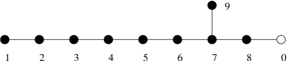
Figure 1: The Dynkin diagram of ${\mathfrak{e}}_{10}$ with the regular $D_{9}$ subalgebra indicated by the solid nodes.

In this section we prepare the analysis of the $E_{10}/K(E_{10})$ $\sigma$-model by studying the decomposition of the hyperbolic KM algebra ${\mathfrak{e}}_{10}$ under its $D_{9}\equiv\mathfrak{so}(9,9)$ subalgebra. This will pave the way for the next section, where we will establish the matching between the equations of motion of the $E_{10}/K(E_{10})$ at the first two levels with the appropriately truncated bosonic equations of motion of $D=11$ supergravity. This matching is analogous to the one obtained w.r.t. the $A_{9}$ decomposition in [13]. The $D_{9}$ decomposition of $E_{10}$ also allows for a simple proof that the second simply-laced maximal rank hyperbolic Kac Moody algebra $DE_{10}$ is actually a proper subalgebra of $E_{10}$ — in agreement with the embedding of type I into type II supergravity.

The (split) algebra ${\mathfrak{e}}_{10}$ is the Kac-Moody algebra defined by the Dynkin diagram of figure 1, where we have marked the nodes which define the regular subalgebra of type $D_{9}$, numbering them from $i=1,...,9$; the remaining node will be labeled by ‘0’. The $D_{9}$ subalgebra appears not in its compact form $\mathfrak{so}(18)$, but via its split form $\mathfrak{so}(9,9)\subset{\mathfrak{e}}_{10}$ — in fact, the compact algebra $\mathfrak{so}(18)$ is not a subalgebra of ${\mathfrak{e}}_{10}$ (whereas $\mathfrak{so}(16)\subset\mathfrak{e}_{8(8)}$ obviously is). The algebra ${\mathfrak{e}}_{10}$ can now be decomposed into an infinite sum of irreducible representations of $\mathfrak{so}(9,9)$. For the determination of the latter one can use the same techniques as the ones that were used in [14] to work out the level decomposition of ${\mathfrak{e}}_{10}$ w.r.t. its $A_{9}$ subalgebra to rather high levels. The results are tabulated in appendix B, which also gives the outer multiplicities of the relevant representations, i.e. the number of times they appear at a given level. Observe that at even levels we have only vectorial representations, whereas at odd levels all $SO(9,9)$ representations are spinorial. Under the $SO(9)\times SO(9)$ subgroup these appear as the product of two spinorial $SO(9)$ representations and therefore as tensorial (single-valued) representations of the diagonal $SO(9)$. We will thus associate the even level representations with the NSNS type fields, and the odd level ones with the RR type fields.

4.1 $E_{10}$ at low levels

We first spell out the relation between the ${\mathfrak{e}}_{10}$ Chevalley generators and the $SO(9,9)$ generators used in the supersymmetric ${\sigma}$-model description. To begin with, we would like to identify the $D_{9}$ Chevalley generators $e_{i},f_{i}$ and $h_{i}$ with $i=1,\ldots,9$ in terms of the $SO(9,9)$ generators $M^{IJ}=-M^{JI}$ obeying the standard commutation relations

$$\left[M^{IJ},M^{KL}\right]=\eta^{KI}M^{JL}-\eta^{KJ}M^{IL}-\eta^{LI}M^{JK}+\eta^{LJ}M^{IK},$$ (4.1)

with

$$\eta^{IJ}={\rm diag}\,\big{[}(+)^{9},(-)^{9}\big{]}\quad\Longleftrightarrow\quad\eta^{ij}={\delta}^{ij}=-\eta^{{\bar{\imath}}{\bar{\jmath}\,}}\;\;;\;\;\eta^{i{\bar{\jmath}\,}}=\eta^{{\bar{\imath}}j}=0$$ (4.2)

where we made use of the $SO(9)\times SO(9)$ indices $I\equiv(i,{\bar{\imath}})$ already introduced before. We use $\eta$ to raise and lower indices in the standard fashion. With the Cartan–Killing form

$$(M^{IJ}|M^{KL})=\eta^{KJ}\eta^{IL}-\eta^{KI}\eta^{JL}$$ (4.3)

we can split the generators into compact and non-compact ones

$$X^{ij}=M^{ij}\quad,\quad X^{{\bar{\imath}}{\bar{\jmath}\,}}=-M^{{\bar{\imath}}{\bar{\jmath}\,}}\quad;\qquad Y^{i{\bar{\jmath}\,}}=M^{i{\bar{\jmath}\,}}.$$ (4.4)

The inner product of the non-compact generators is then

$$(Y^{i{\bar{\jmath}\,}}|Y^{k{\bar{l}}})={\delta}^{ik}{\delta}^{{\bar{\jmath}\,}{\bar{l}}}.$$ (4.5)

The $\mathfrak{so}(9,9)$ Chevalley generators are obtained by setting (recall that ${\bar{\imath}}\equiv i+8$, etc.)

$$e_{i} = \frac{1}{2}\Big{(}M^{\overline{i+1},{\bar{\imath}}}-M^{i+1,i}+M^{i+1,{\bar{\imath}}}-M^{\overline{i+1},i}\Big{)}$$ (4.6a)

$$f_{i} = \frac{1}{2}\Big{(}M^{i+1,{\bar{\imath}}}-M^{\overline{i+1},i}-M^{\overline{i+1},{\bar{\imath}}}+M^{i+1,i}\Big{)}$$ (4.6b)

$$h_{i} = M^{i+1,\overline{i+1}}-M^{i,{\bar{\imath}}}$$ (4.6c)

for $i=1,\ldots,8$ and

$$e_{9} = \frac{1}{2}\Big{(}M^{\overline{9},\overline{8}}+M^{9,8}-M^{9,\overline{8}}-M^{\overline{9},8}\Big{)}$$ (4.7a)

$$f_{9} = -\frac{1}{2}\Big{(}M^{9,\overline{8}}+M^{\overline{9},8}+M^{\overline{9},\overline{8}}+M^{9,8}\Big{)}$$ (4.7b)

$$h_{9} = -M^{8,\overline{8}}-M^{9,\overline{9}}.$$ (4.7c)

With the $SO(9,9)$ commutation relations given above it is straightforward to check that they indeed satisfy the generating relations. Furthermore, the standard invariant bilinear form is precisely the one given by (4.3).

The remaining independent generator at level $\ell=0$ is the Cartan subalgebra generator $T$ corresponding to the fundamental weight $\lambda_{0}$ associated to the node marked $0$ in figure 1, whose explicit form is

$$T=-h_{1}-2h_{2}-3h_{3}-4h_{4}-5h_{5}-6h_{6}-7h_{7}-\frac{9}{2}h_{8}-\frac{7}{2}h_{9}-2h_{0}.$$ (4.8)

It generates a $GL(1)\equiv{\mathbb{R}}^{+}$ subgroup which commutes with and is orthogonal to the $\mathfrak{so}(9,9)$ subalgebra, and is normalized according to

$$(T|M^{IJ})=0,\quad,\qquad(T|T)=-1.$$ (4.9)

The maximal compact subalgebra is the invariant subalgebra w.r.t. the Chevalley involution

$${\omega}(e_{i})=-f_{i}\;\;,\quad{\omega}(f_{i})=-e_{i}\;\;,\quad{\omega}(h_{i})=-h_{i}\;\;;\quad$$ (4.10)

and is therefore spanned by the multiple commutators of the $(e_{i}-f_{i})$. From

$$e_{i}-f_{i} = M^{\overline{i+1},{\bar{\imath}}}-M^{i+1,i}{}$$

$$e_{9}-f_{9} = M^{\bar{9},\bar{8}}+M^{9,8}.$$ (4.11a)

we see that the combinations $(e_{8}-f_{8})\pm(e_{9}-f_{9})$ are Lorentz generators solely containing barred $M^{\bar{9},\bar{8}}$ or unbarred indices $M^{9,8}$, respectively. Under further commutation with the remaining $(e_{i}-f_{i})$ we can thus obtain any Lorentz generator with only barred or unbarred indices. This identifies the maximal compact subalgebra as $\mathfrak{so}(9)\oplus\mathfrak{so}(9)$, as anticipated.

Performing a decomposition of ${\mathfrak{e}}_{10}$ into representations of $\mathfrak{so}(9,9)$ we obtain the table given in appendix B whose first four entries we reproduce here for convenience. (All fields occur with outer multiplicity one.)

$\ell$	$[p_{1}\ldots p_{9}]$	$SO(9,9)$ generator	Transposed generator at level $-\ell$
0	[010000000]	$M^{IJ}$	$M_{IJ}={\omega}(M^{IJ})$
0	[000000000]	$T$	$T$
1	[000000010]	$E_{A}$	$F_{\dot{A}}$
2	[001000000]	$E^{IJK}$	$F_{IJK}$

Having already discussed $\ell=0$ above, we see from the table, there is only one representation at level $\ell=1$, with Dynkin label $[000000001]$. This is the ${\bf 256_{s}}$ spinor representation $E_{A}$ of $\mathfrak{so}(9,9)$; the Chevalley generator $e_{0}$ of ${\mathfrak{e}}_{10}$ corresponds to the highest weight state of this representation. The components of the spinor $E_{A}$ carry $GL(1)$ charge $\frac{1}{2}$ with our choice for $T$. Using the Weyl spinor notation of appendix A, we thus have

$$\left[M^{IJ},E_{A}\right] = -{\textstyle{\frac{1}{2}}}{\Sigma}^{IJ}_{AB}E_{B},$$ (4.12a)

$$\left[T,E_{A}\right] = {\textstyle{\frac{1}{2}}}E_{A}.$$ (4.12b)

The conjugate generators $-{\omega}(E_{A})={\cal C}_{A{\dot{B}}}F_{\dot{B}}$ at level $\ell=-1$ belong to the conjugate spinor representation $\bf{256}_{c}$. This follows from the fact that the Chevalley involution reverses chirality, which itself is a consequence of the fact that the chirality operator $\widehat{\Gamma}^{*}$ (see appendix A) is represented as the product over an odd number of Cartan subalgebra generators in terms of $\widehat{\Gamma}^{IJ}$, which implies

$${\omega}(h_{1}\cdots h_{9})=-h_{1}\cdots h_{9}$$ (4.13)

which in turn requires that on the spinor representations

$${\omega}(\widehat{\Gamma}^{*})=-\widehat{\Gamma}^{*}$$ (4.14)

Using dotted indices, we have the commutation relations

$$\left[M^{IJ},F_{{\dot{A}}}\right] = -{\textstyle{\frac{1}{2}}}\bar{{\Sigma}}^{IJ}_{{\dot{A}}{\dot{B}}}F_{{\dot{B}}},$$ (4.15a)

$$\left[T,F_{{\dot{A}}}\right] = -{\textstyle{\frac{1}{2}}}F_{{\dot{A}}}.$$ (4.15b)

The commutator of level $\ell=1$ with level $\ell=-1$ is

$$\left[E_{A},F_{{\dot{B}}}\right] = \frac{1}{4}({\Sigma}^{IJ}{\cal C})_{A{{\dot{B}}}}M_{IJ}-\frac{1}{2}{\cal C}_{A{{\dot{B}}}}T,$$ (4.16)

where the constants are determined from the inner product of these fields within ${\mathfrak{e}}_{10}$

$$(E_{A}|F_{{\dot{B}}})={\cal C}_{A{\dot{B}}}.$$ (4.17)

At $\ell=2$ we have the $\mathfrak{so}(9,9)$ representation with Dynkin label $[001000000]$, i.e. a 3-form generator $E^{IJK}$ with commutation relations

$$\left[M^{IJ},E^{KLM}\right] = 3\eta^{I[K}E^{LM]J}-3\eta^{J[K}E^{LM]I},$$ (4.18a)

$$\left[T,E^{KLM}\right] = E^{KLM}.$$ (4.18b)

It is generated by taking the commutator of two $\ell=1$ generators

$$\left[E_{A},E_{B}\right] = \frac{1}{6}({{\Sigma}}_{IJK}{\bar{\cal C}})_{AB}E^{IJK}.$$ (4.19)

Note that ${\Sigma}^{IJK}{\bar{\cal C}}$ is indeed antisymmetric as required for consistency. The transposed field

$$F_{IJK}:=-\omega(E^{IJK})$$ (4.20)

(note the position of indices) satisfies

$$\left[M^{IJ},F^{KLM}\right] = 3\eta^{I[K}F^{LM]J}-3\eta^{J[K}F^{LM]I}$$ (4.21a)

$$\left[T,F^{KLM}\right] = -F^{KLM}$$ (4.21b)

$$\left[F_{{\dot{A}}},F_{{\dot{B}}}\right] = -\frac{1}{6}(\bar{{\Sigma}}^{IJK}{\cal C})_{{\dot{A}}{\dot{B}}}F_{IJK}$$ (4.21c)

To determine the proper normalization of the level 2 generators, we observe that the combination

$$v=E^{123}+E^{\bar{1}23}+E^{1\bar{2}3}+E^{12\bar{3}}+E^{1\bar{2}\bar{3}}+E^{\bar{1}2\bar{3}}+E^{\bar{1}\bar{2}3}+E^{\bar{1}\bar{2}\bar{3}}\;,$$ (4.22)

is the lowest weight vector of the representation with basis elements $E^{IJK}$. Normalizing it according to $-(v|{\omega}(v))=1$ we deduce the inner product of $E^{IJK}$ and $F_{LMN}$

$$(E^{IJK}|F_{LMN}) = \frac{3}{4}\,\delta^{IJK}_{LMN},$$ (4.23)

This normalization was also used to fix the constants in (4.19) and (4.21c).

The remaining commutators up to level $\ell=2$ are

$$\left[E^{IJK},F_{\dot{A}}\right] = \frac{1}{8}{\Sigma}^{IJK}_{B{\dot{A}}}E_{B},$$ (4.24a)

$$\left[F^{IJK},E_{A}\right] = -\frac{1}{8}\bar{{\Sigma}}^{IJK}_{{\dot{B}}A}F_{\dot{B}},$$ (4.24b)

$$\left[E^{IJK},F_{LMN}\right] = -\frac{3}{4}\,{\delta}^{IJK}_{LMN}T-\frac{9}{4}{\delta}^{[IJ}_{[LM}{M^{K]}}_{N]}.$$ (4.24c)

Finally, let us have a look at the ‘affine representations’ analogous to those identified in [13], and proposed there to be associated to the spatial gradients. In the present decomposition, they are ($n\geq 0$)

$$\ell=2n+1\qquad \longleftrightarrow \qquad[n00000010]$$ (4.25a)

$$\ell=2n+2\qquad \longleftrightarrow \qquad[n01000000]$$ (4.25b)

Like the corresponding representations in [13], they appear all with outer multiplicity one. Trying a similar interpretation, we are led to associate ($I=1,\ldots,18$)

$${\partial}_{I_{1}}\cdots{\partial}_{I_{n}}P_{{\alpha}{\bar{\alpha}}}\qquad \longleftrightarrow \qquad[n00000010],$$ (4.26a)

$${\partial}_{I_{1}}\cdots{\partial}_{I_{n}}P_{JKL}\qquad \longleftrightarrow \qquad[n01000000],$$ (4.26b)

since the generator $E_{A}-{\cal C}_{A{\dot{A}}}F_{\dot{A}}$ multiplies a field strength $P^{A}=P_{{\alpha}{\bar{\alpha}}}$ under $SO(9)\times SO(9)$. As these are representations of $SO(9,9)$ they come with an additional tracelessness constraint, for example

$$\hat{{\Gamma}}^{I}_{{\alpha}{\bar{\alpha}}\,{\beta}{\bar{\beta}}}{\partial}_{I}P_{{\beta}{\bar{\beta}}}=0.$$ (4.27)

Notice that these are now 18-dimensional ‘gradients’, and therefore an interpretation along the lines of [13] is more subtle. Splitting the $18$ components into $9+9$, and recalling that the two $SO(9)$ groups act on left and right moving sectors of the superstring, respectively, we are led to tentatively associate these representations to the derivatives w.r.t. the left and right moving target space coordinates $x^{i}$ and $x^{\bar{\imath}}=\tilde{x}^{i}$ (where the latter are defined by the worldsheet duality relation ${\partial}_{\pm}x^{i}=\pm{\partial}_{\pm}\tilde{x}^{i}$). We see no direct trace of the derivatives w.r.t. the circle in the eleventh direction, but we know from the $GL(10)$ analysis of [13] that they are present.

4.2 Type I $\subset$ Type II, and $DE_{10}\subset E_{10}$

Type I supergravity is a subsector of the type II theory and is conjectured to possess a hidden Kac–Moody symmetry $DE_{10}$ in one dimension [4]. The Dynkin diagram of the hyperbolic over-extension $DE_{10}=D_{8}^{++}$ is displayed in figure 2. Here we show that the conjectured $DE_{10}$ symmetry is completely consistent with the $E_{10}$ symmetry of the type IIA theory by proving that $\mathfrak{de}_{10}$ is a subalgebra of ${\mathfrak{e}}_{10}$ . More specifically, the elements $DE_{10}$ form a subset of the NSNS sector of $E_{10}$, corresponding to the even levels in the $D_{9}$ decomposition of $E_{10}$. We note that the analogous embedding of $DE_{11}$ into $E_{11}$ was recently established in [27] also by invoking the embedding of type I into type IIA supergravity, but the level decomposition via their common $D_{10}$ has so far not been studied in any detail.

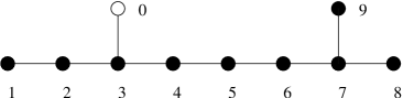
Figure 2: The Dynkin diagram of $DE_{10}=D_{8}^{++}$ with the regular $D_{9}$ subalgebra indicated by the solid nodes. This subalgebra is identical to the one of $E_{10}$ in figure 1.

It is evident from figure 2 that $DE_{10}$ has a regular $D_{9}$ subalgebra, and therefore also admits a decomposition into $SO(9,9)$ tensors. To facilitate the comparison with $E_{10}$, we have chosen the same labeling conventions for both Dynkin diagrams. In order to distinguish the two decompositions, we will in this subsection denote by $\ell^{D}$ the level in the decomposition of $DE_{10}$ with respect to $D_{9}$ and by $\ell^{E}$ the level of the $E_{10}$ decomposition. The level $\ell^{E}=\ell^{D}=0$ sectors contain the adjoint of $\mathfrak{so}(9,9)$ and a scalar in both decompositions. Since we tentatively identified these fields in the $E_{10}$ decomposition with the type I fields, the two $\mathfrak{so}(9,9)$ are naturally identified. In order to retrieve $DE_{10}$ in $E_{10}$ all that remains to be done is to identify the simple root ${\alpha}_{0}^{D}$ of $DE_{10}$ as a real root in the $E_{10}$ root lattice; the subalgebra property is then a simple consequence of Thm. 3.1 of [45].

The type I fields are (contained in) the NSNS fields which belong to the even levels $\ell^{E}\in 2{\mathbb{Z}}$ of the $E_{10}$ decomposition. The only representation at level $\ell^{E}=2$ has Dynkin labels $[001000000]$ and is generated by a highest weight vector in the root space of

$${\alpha}_{0}^{D}\equiv{\alpha}_{4}+2{\alpha}_{5}+3{\alpha}_{6}+4{\alpha}_{7}+3{\alpha}_{8}+2{\alpha}_{9}+2{\alpha}_{0}^{E}=:2{\alpha}_{0}+\sum_{i=1}^{9}n_{i}{\alpha}_{i}$$ (4.28)

in the $E_{10}$ root lattice. This formula is easily read off from the list of highest weight vectors (see appendix B), and it is also easy to check that ${\alpha}_{0}^{D}$ is a real root. This root also appeared in [27] in the context of very-extended symmetries of type I theories as a subsector of type II. We can thus adjoin this root to the nine (common) simple roots of $\mathfrak{so}(9,9)$ called ${\alpha}_{i}$ ($i=1,\ldots,9$). Using the inner product in $E_{10}$ one verifies that their inner product matrix is just the Cartan matrix of $DE_{10}$; hence, the ten elements ${\alpha}_{0}^{D}$, ${\alpha}_{i}$ constitute a set of simple roots within $E_{10}$ as none of their differences is a root. Therefore [45], they generate a subalgebra of $E_{10}$ which is just $DE_{10}$. This could have been guessed already by inspection of the $DE_{10}$ diagram, where the representation at $\ell^{D}=1$ corresponding to the simple root ${\alpha}_{0}^{D}$ is easily is seen to be $[001000000]$, which is also the only representation appearing at level $\ell^{E}=2$ for $E_{10}$.

We note a few immediate consequences of the embedding $DE_{10}\subset E_{10}$. First of all, if a root ${\alpha}$ is a root of both $DE_{10}$ and $E_{10}$, and therefore belongs to the root lattice of $DE_{10}$ embedded in the $E_{10}$ root lattice, the multiplicity of ${\alpha}$ as root of $DE_{10}$ cannot exceed its multiplicity as an $E_{10}$ root

$${\rm mult}_{DE_{10}}(\alpha)\leq{\rm mult}_{E_{10}}(\alpha).$$ (4.29)

We recall that the condition for a positive $DE_{10}$ root ${\alpha}=\sum_{a=0}^{9}m_{a}^{D}{\alpha}_{a}^{D}$ to contain a highest weight vector for a $\mathfrak{so}(9,9)$ representation with Dynkin labels $[p_{1}\ldots p_{9}]$ at level $\ell^{D}=m_{0}^{D}$ is [13, 14]

$$m_{i}^{D}=-\sum_{j=1}^{9}S^{-1}_{ij}p_{j}+S^{-1}_{i3}\ell^{D},$$ (4.30)

for $i=1,\ldots,9$, where $S$ is the Cartan matrix of $D_{9}$. Similarly, the condition for $E_{10}$ and the same representation is

$$m_{i}^{E}=-\sum_{j=1}^{9}S^{-1}_{ij}p_{j}+S^{-1}_{i9}\ell^{E}.$$ (4.31)

Subtracting the two conditions, and using $\ell^{E}=2\ell^{D}$ from the explicit form in (4.28), we find

$$m_{i}^{E}=m_{i}^{D}+\ell^{D}n_{i},$$ (4.32)

in agreement with the embedding of the lattices. Consequently, any admissible representation in the $DE_{10}$ decomposition yields an allowed representation in the $E_{10}$ representation. The converse can be shown to be true using the hyperbolicity of $DE_{10}$.

Using the embedding it is also evident that for each admissible representation of both $DE_{10}$ and $E_{10}$, the outer multiplicities obey an inequality analogous to (4.29), namely

$${\mu}_{DE_{10}}({\alpha})\leq{\mu}_{E_{10}}({\alpha}).$$ (4.33)

This inequality follows from the fact that all representations in $DE_{10}$ are obtained from commutation of the $\ell^{D}=1$ representation and this representations is present on $\ell^{E}=2$ in $E_{10}$ obeying the same commutation relations. Additional fields in $E_{10}$ can arise by taking commutators of odd level elements into account, thereby increasing the outer multiplicity compared to its value in $DE_{10}$ decomposition. The effect of these additional fields in view of (4.33) can be studied in the tables of appendices B and C.

As a ten dimensional string theory, type I is obtained from type IIA by gauging a combination between world-sheet parity and space-time parity. (This breaks the Poincaré symmetry in ten dimensions; also clear since the $32$ D8-branes required for the only consistent $SO(32)$ gauge group, act as domain walls. Actually, one should start from IIB but after compactification they are equivalent anyway.) This parity is seen to leave all the NSNS-fields intact and we can study (at least empirically) the question if the type I NSNS fields are all fields on the even levels of $E_{10}$ decomposed with respect to $\mathfrak{so}(9,9)$. (Algebraically, this question is equivalent to studying the obvious subalgebra given by all even levels $\ell^{E}\in 2{\mathbb{Z}}$ and asking whether it is identical to $DE_{10}$.) From the tables in appendices B and C, it is apparent that there are fields in $E_{10}$ which qualify as NSNS fields but which do not derive from the type I subalgebra. An example of such a field is the representation $[000000100]$ on level $\ell^{E}=6$ ($\ell^{D}=3$). Assuming the validity of $E_{10}$ as a symmetry of M-theory we can therefore learn something about the additional degrees of freedom from studying these tables.

Finally, we note that the decomposition of $E_{10}$ under its regular $A_{9}$ subalgebra, as studied in [13, 14], can be used to establish that (the non-hyperbolic, over-extended) $AE_{10}$ is a subalgebra of $E_{10}$ as well. This was already shown in [32] for all very-extended algebras where this subalgebra corresponded to the gravity subsector of the generalised M-theories. The new simple root is now

$${\alpha}_{0}^{A}={\alpha}_{3}+2{\alpha}_{4}+3{\alpha}_{5}+4{\alpha}_{6}+5{\alpha}_{7}+3{\alpha}_{8}+{\alpha}_{9}+3{\alpha}_{0}^{E}$$ (4.34)

As in [32], $AE_{10}$ is associated with the gravity sector here, too (see also [6]). The levels containing fields belonging to that subalgebra are multiples of three: $\ell=3n$. The embedding $AE_{10}\subset E_{10}$ implies inequalities analogous to (4.29) and (4.33).

5 $E_{10}/K(E_{10})$ coset space dynamics

5.1 The $E_{10}/K(E_{10})$ ${\sigma}$-model at levels $\ell=0,\pm 1$

In [13] it was shown that a truncated version of the $D=11$ supergravity equations of motion, where one retains only the fields and their first order spatial gradients, can be mapped onto a constrained null geodesic motion in the infinite dimensional coset space $E_{10}({\mathbb{R}})/K(E_{10})$. The detailed comparison there was based on a level expansion in terms of the $A_{9}$ subalgebra of ${\mathfrak{e}}_{10}$ up to level $\ell=3$, or alternatively up to height 30 in the roots of ${\mathfrak{e}}_{10}$. Here, we will repeat this analysis, but now in terms of the level expansion of ${\mathfrak{e}}_{10}$ w.r.t. its $D_{9}$ subalgebra, using the results of the foregoing sections. While the $A_{9}$ decomposition is appropriate to the direct reduction from eleven to one dimensions, with the $GL(10)$ global symmetry acting in the obvious way on the spatial zehnbein, the $D_{9}$ decomposition is linked to the reduction of the IIA theory from ten to one dimensions, and hence by duality also to the type IIB theory, as we have explained. Apart from technical differences, such as the appearance of spinor representations of $D_{9}$ at odd levels, the $D_{9}$ decomposition thus provides a different, and more ‘stringy’ perspective, because the group $SO(9,9,{\mathbb{Z}})$ is the T-duality symmetry known to arise in the compactification of the IIA superstring to one dimension. Indeed, extra work was required to bring the dimensionally reduced Lagrangian into an $SO(9,9)$ resp. $SO(9)\times SO(9)$ invariant form, because only the global $SL(9,{\mathbb{R}})\subset SO(9,9)$ and the local $SO(9)\equiv{\rm diag}\,[SO(9)\times SO(9)]$ are manifest in the dimensional reduction. Accordingly, the $\ell=0$ sector already contains part of the 3-form field $A_{MNP}$, whereas in the $A_{9}$ decomposition it only contains the metric (zehnbein) degrees of freedom. Here, we will analyse the $\ell=0,1$ sector, and perform some partial checks for the $\ell=2$ sector.

For this purpose, we slightly adapt the method of [13]: we will not use a background metric in order to be able to avoid having to introduce a ‘spinorial metric’ to deal with the odd level spinorial representations (for the $A_{9}$ decomposition this problem does not arise because $SL(10)$ does not have spinorial representations). Let us also emphasize once more that the identification of the relevant ${\sigma}$-model quantities (cf. (5.1) below) with the corresponding field strengths of $D=11$ supergravity was derived via an analysis of the supersymmetry transformations, so the comparison with the bosonic equations of motion we are about to perform serves as an additional consistency check.

As for finite dimensional ${\sigma}$-models, we describe the bosonic degrees of freedom in terms of a ‘matrix’ ${\cal V}(t)\in E_{10}$ depending on one time parameter $t$. The quantity ${\partial_{t}}{\cal V}{{\cal V}}^{-1}$ then belongs to the Lie algebra ${\mathfrak{e}}_{10}$ and can be decomposed into a connection ${\cal Q}$ in the maximal compact subalgebra $\mathfrak{ke}_{10}$, and a coset component ${\cal P}$:

$${\partial_{t}}{\cal V}{\cal V}^{-1}={\cal Q}+{\cal P}.$$ (5.1)

In order to make the grading and dilaton dependence more explicit, we parametrize the coset element as

$${\cal V}=e^{{\varphi}T}\tilde{{\cal V}}$$ (5.2)

by factoring out the dilaton. With this definition, the terms at level $\ell$ in (5.1) will be dressed with an explicit factor $e^{\frac{\ell}{2}{\varphi}}$. In a triangular gauge, where the ${\cal V}$ is the exponential of a Borel subalgebra with only contributions from levels $\ell\geq 0$, we thus obtain

$${\partial_{t}}{\cal V}{\cal V}^{-1} = {\partial_{t}}{\varphi}\cdot T+e^{{\varphi}T}\big{(}{\partial_{t}}\tilde{\cal V}\tilde{\cal V}^{-1}\big{)}e^{-{\varphi}T}{}$$ (5.3)

$$= {\partial_{t}}{\varphi}\cdot T+P_{i{\bar{\jmath}\,}}Y^{i{\bar{\jmath}\,}}+e^{\frac{1}{2}{\varphi}}P^{(1)}_{A}E^{A}+e^{{\varphi}}P^{(2)}_{IJK}E^{IJK}+\dots$$

where the dots stand for higher level contributions which we neglect, and the superscripts indicate the level for $\ell>0$. Splitting the terms on the r.h.s. according to whether they belong to the compact subalgebra or the coset, we get

$${\cal Q} = {\textstyle{\frac{1}{2}}}Q_{ij}X^{ij}+{\textstyle{\frac{1}{2}}}Q_{{\bar{\imath}}{\bar{\jmath}\,}}X^{{\bar{\imath}}{\bar{\jmath}\,}}+{\textstyle{\frac{1}{2}}}e^{{\textstyle{\frac{{\varphi}}{2}}}}P^{(1)}_{A}(E_{A}-{\cal C}_{A{\dot{B}}}F_{\dot{B}})+{\textstyle{\frac{1}{2}}}e^{\varphi}P^{(2)}_{IJK}(E^{IJK}-F_{IJK})+\dots$$

$${\cal P} = {\partial_{t}}{\varphi}\cdot T+P_{i{\bar{\jmath}\,}}Y^{i{\bar{\jmath}\,}}+{\textstyle{\frac{1}{2}}}e^{{\textstyle{\frac{{\varphi}}{2}}}}P^{(1)}_{A}(E_{A}+{\cal C}_{A{\dot{B}}}F_{\dot{B}})+{\textstyle{\frac{1}{2}}}e^{\varphi}P^{(2)}_{IJK}(E^{IJK}+F_{IJK})+\dots$$ (5.4)

For any variation along the coset

$${\delta}{\cal V}{\cal V}^{-1}={\Lambda}\equiv{\Lambda}_{i{\bar{\jmath}\,}}Y^{i{\bar{\jmath}\,}}+{\textstyle{\frac{1}{2}}}{\Lambda}_{A}(E_{A}+{\cal C}_{A{\dot{B}}}F_{\dot{B}})+{\textstyle{\frac{1}{2}}}{\Lambda}_{IJK}(E^{IJK}+F_{IJK})\dots,$$ (5.5)

with $-{\omega}({\Lambda})={\Lambda}$, we therefore have

$${\delta}\left({\partial_{t}}{\cal V}{\cal V}^{-1}\right)={\partial_{t}}{\Lambda}-[{\cal Q},{\Lambda}]-[{\cal P},{\Lambda}]$$ (5.6)

Thus, the local supersymmetry variations at levels $\ell=0$ and $\ell=1$ are identified as follows, cf. (3.53) and (3.84),

$${\Lambda}_{i{\bar{\jmath}\,}} = i\varepsilon_{\alpha}{\gamma}_{i{\alpha}{\beta}}\chi_{{\bar{\jmath}\,}{\beta}}+i\varepsilon_{\bar{\alpha}}{\gamma}_{{\bar{\jmath}\,}{\bar{\alpha}}{\bar{\beta}}}\chi_{i{\bar{\beta}}}$$ (5.7a)

$${\Lambda}_{A} = {\Lambda}_{{\alpha}{\bar{\alpha}}}=2i\Big{[}\varepsilon_{\alpha}\chi_{\bar{\alpha}}-\varepsilon_{\bar{\alpha}}\chi_{\alpha}+\varepsilon_{\beta}{\gamma}_{i{\beta}{\alpha}}\chi_{i{\bar{\alpha}}}-\varepsilon_{\bar{\beta}}{\gamma}_{{\bar{\jmath}\,}{\bar{\beta}}{\bar{\alpha}}}\chi_{{\bar{\jmath}\,}{\alpha}}\Big{]},$$ (5.7b)

where we have rewritten the $SO(9,9)$ spinor as an $({\bf 16},{\bf 16})$ bispinor under $SO(9)\times SO(9)$ as before. The above formulae are convenient both for deriving the equations of motion as well as keeping track of the dilaton dependence in the variations of the $P$’s. For instance, we have

$${\delta}P_{i{\bar{\jmath}\,}} = D_{t}{\Lambda}_{i{\bar{\jmath}\,}}{}$$

$${\delta}\big{(}e^{\frac{1}{2}{\varphi}}P_{A}^{(1)}E^{A}\big{)} = D_{t}{\Lambda}_{A}E^{A}+\frac{1}{2}e^{\frac{1}{2}{\varphi}}\big{[}P_{A}^{(1)}(E^{A}-{\cal C}^{A{\dot{B}}}F_{\dot{B}})\,,\,{\Lambda}_{i{\bar{\jmath}\,}}Y^{i{\bar{\jmath}\,}}\big{]}+\dots$$ (5.8)

The (bosonic) null geodesic motion in $E_{10}/K(E_{10})$ is governed by the Lagrange function [13]

$${\cal L}=\frac{1}{4}n^{-1}({\cal P}|{\cal P})$$ (5.9)

which gives rise to the $K(E_{10})$-covariant equations of motion in the standard fashion:

$${\cal D}_{t}(n^{-1}{\cal P})\equiv{\partial_{t}}(n^{-1}{\cal P})-n^{-1}[{\cal Q},{\cal P}]=0.$$ (5.10)

Since we understand the Kac–Moody algebra ${\mathfrak{e}}_{10}$ at the very lowest levels only, we truncate the expansion (5.1) and the evaluation of (5.10) after some level to obtain an approximation to the dynamics. Notice that the higher level terms come with additional powers of the ‘string coupling’ $e^{\frac{1}{2}{\varphi}}$ (recall, however, that our dilaton is different from the standard IIA string dilaton), which would be suppressed for $\langle{\varphi}\rangle<0$. In order to write the equations of motion we explicitly covariantize with respect to $SO(9)\times SO(9)$ by replacing ${\partial_{t}}$ by the $SO(9)\times SO(9)$ covariant $D_{t}$ and leaving out the contribution from $Q_{ij}$ and $Q_{{\bar{\imath}}{\bar{\jmath}\,}}$ on the r.h.s. of (5.10). This results in expressions like (3.57) for spinor and vector indices.

The expansion of the coset Lagrange function up to level $\ell=1$ yields

$${\cal L}=\frac{1}{4}n^{-1}\Big{(}P_{i{\bar{\jmath}\,}}P_{i{\bar{\jmath}\,}}-({\partial_{t}}{\varphi})^{2}\Big{)}+\frac{1}{8}n^{-1}e^{\varphi}P_{{\alpha}{\bar{\alpha}}}P_{{\alpha}{\bar{\alpha}}}\;,$$ (5.11)

and this agrees indeed with the first line of the reduced type II Lagrangian (3.85). Note that $P_{A}^{(1)}=P_{{\alpha}{\bar{\alpha}}}$ is to be expanded in terms of odd degree ${\gamma}$-matrices since all ${\varphi}$-dependence resides in the prefactor $e^{\varphi}$.

From (5.10) we can derive the $\sigma$-model equations of motion for levels $\ell\leq 1$, and compare them with those of massive IIA supergravity. The bosonic equations of motion at levels $\ell=0,1$ that follow from (5.10), with contributions up to $|\ell|=2$, read

$${\partial}_{t}\big{(}n^{-1}{\partial_{t}}{\varphi}\big{)} = -\frac{1}{4}n^{-1}e^{\varphi}P_{{\alpha}{\bar{\alpha}}}P_{{\alpha}{\bar{\alpha}}}+$$

$$\qquad+\frac{1}{24}n^{-1}e^{2{\varphi}}\Big{(}P_{ijk}P_{ijk}-3P_{ij{\bar{k}}}P_{ij{\bar{k}}}+3P_{i{\bar{\jmath}\,}{\bar{k}}}P_{i{\bar{\jmath}\,}{\bar{k}}}-P_{{\bar{\imath}}{\bar{\jmath}\,}{\bar{k}}}P_{{\bar{\imath}}{\bar{\jmath}\,}{\bar{k}}}\Big{)}+\ldots{}$$

$$D_{t}\big{(}n^{-1}P_{i{\bar{\jmath}\,}}\big{)} = \frac{1}{4}n^{-1}e^{\varphi}{\gamma}^{i}_{{\alpha}{\beta}}{\gamma}^{\bar{\jmath}\,}_{{\bar{\alpha}}{\bar{\beta}}}P_{{\alpha}{\bar{\alpha}}}P_{{\beta}{\bar{\beta}}}-$$

$$\qquad-\frac{1}{4}n^{-1}e^{2{\varphi}}\Big{(}P_{ikl}P_{{\bar{\jmath}\,}kl}-2P_{ik{\bar{l}}}P_{{\bar{\jmath}\,}k{\bar{l}}}+P_{i{\bar{k}}{\bar{l}}}P_{{\bar{\jmath}\,}{\bar{k}}{\bar{l}}}\Big{)}+\ldots{}$$

$$D_{t}\big{(}n^{-1}e^{\varphi}P_{{\alpha}{\bar{\alpha}}}\big{)} = \frac{1}{2}{\gamma}^{i}_{{\alpha}{\beta}}{\gamma}^{\bar{\jmath}\,}_{{\bar{\alpha}}{\bar{\beta}}}n^{-1}e^{\varphi}P_{i{\bar{\jmath}\,}}P_{{\beta}{\bar{\beta}}}+$$

$$\!\!\!\!\!\!\!\!\!\!\!\!\!\!\!\!\!\!\!\!\!\!\!\!\!\!\!\!\!\!\!\!\!\!\!\!\!\!\!\!\!\!\!\!\!\!+\frac{1}{8}n^{-1}e^{2{\varphi}}P_{{\beta}{\bar{\beta}}}\Big{(}-P_{ijk}{\gamma}^{ijk}_{{\alpha}{\beta}}{\delta}_{{\bar{\alpha}}{\bar{\beta}}}+3P_{ij{\bar{k}}}{\gamma}^{ij}_{{\alpha}{\beta}}{\gamma}^{\bar{k}}_{{\bar{\alpha}}{\bar{\beta}}}-3P_{i{\bar{\jmath}\,}{\bar{k}}}{\gamma}^{i}_{{\alpha}{\beta}}{\gamma}^{{\bar{\jmath}\,}{\bar{k}}}_{{\bar{\alpha}}{\bar{\beta}}}+P_{{\bar{\imath}}{\bar{\jmath}\,}{\bar{k}}}{\gamma}^{{\bar{\imath}}{\bar{\jmath}\,}{\bar{k}}}_{{\bar{\alpha}}{\bar{\beta}}}{\delta}_{{\alpha}{\beta}}\Big{)}+\dots$$

where we have now dropped the superscripts indicating the level for simplicity of notation, and where, for instance, the last line is obtained by expanding out $\Gamma^{IJK}_{AB}P^{(1)}_{B}P^{(2)}_{IJK}$ in terms of $SO(9)\times SO(9)$ indices. We have included the $\ell=2$ contributions for completeness but will only make partial use of these terms when relating (5.12) to the reduced massive ${\rm IIA}$ equations of motion.

5.2 Equivalence to type II supergravity

For the comparison with massive IIA supergravity, we first note that the correctness of the $\ell=0$ truncation already follows from our rewriting of the reduced Lagrangian into ${\sigma}$-model form. In particular, the $SO(9)\times SO(9)$ covariant derivative $D_{t}$ takes care not only of the terms involving the spin connection, but also the couplings of the NSNS field $A_{mn{\widetilde{10}}}$.

We will now demonstrate in examples that the ${\sigma}$-model equations (5.12) coincide with the various components of the bosonic $D=11$ supergravity equations of motion (2.3) and the Bianchi identities (2.4). For the latter we will use flat indices, which results in extra contributions from the spatial components of the spin connection, as in (3.74). For the contributions generated by the Romans mass $M$, we merely check the couplings against the results of [15], but not the precise numerical coefficients.

At level $\ell=0$, we deduce the following equations of motion for $P_{i{\bar{\jmath}\,}}$ and ${\varphi}$ from our definitions (3.43),

$$\frac{1}{2}nD_{t}\big{(}n^{-1}(P_{i{\bar{\jmath}\,}}+P_{j{\bar{\imath}}})\big{)} = -N^{2}\big{(}R_{ij}+\frac{1}{2}{\delta}_{ij}R_{10,10}-2e_{i}{}^{m}e_{j}{}^{n}g^{pq}F_{tmp{\widetilde{10}}}F_{tnq{\widetilde{10}}}\big{)},$$ (5.13a)

$$\frac{1}{2}nD_{t}\big{(}n^{-1}(P_{i{\bar{\jmath}\,}}-P_{j{\bar{\imath}}})\big{)} = -n{\partial_{t}}\big{(}n^{-1}g^{mp}g^{nq}F_{tpq{\widetilde{10}}}\big{)},$$ (5.13b)

$$n{\partial_{t}}\big{(}n^{-1}{\partial_{t}}{\varphi}\big{)} = -N^{2}\big{(}-\frac{3}{2}R_{10,10}-{\delta}^{ab}R_{ab}\big{)}.$$ (5.13c)

We have separated the symmetric and anti-symmetric part of the equation for $P_{i{\bar{\jmath}\,}}$ since it is clear from (3.43) that the first will correspond to Einstein’s equation of motion while the latter should reduce to the equation for the NSNS 2-form. It is easy to check from (2.3) that they are equivalent to the vanishing of the equations (5.13) if one considers only contributions from $\ell=0$. Note that the combination of Ricci tensors in (5.13a) is correct in that it cancels contributions of the form ${\delta}_{ij}g^{mn}g^{pq}F_{tmp{\widetilde{10}}}F_{tnq{\widetilde{10}}}$ from (2.3b) as required, since (5.12) does not have any such trace terms. The contribution to (5.13a) from the RR fields at $\ell=1$ on the r.h.s. of (5.12) yields, taking $G_{tmnp}$ as an example,

$$-n^{-1}e^{\varphi}g^{\frac{1}{2}}g^{mn}g^{pq}G_{timp}G_{tjnq}+\frac{1}{6}n^{-1}e^{\varphi}g^{\frac{1}{2}}{\delta}_{ij}g^{mn}g^{pq}g^{rs}G_{tmpr}G_{tnqs}.$$ (5.14)

(note the appearance of the redefined field strength (3.72)). This coincides indeed with the corresponding term on the r.h.s. of Einstein’s equations (2.3b). The other contributions work analogously.

To analyse the $\ell=1$ equations for $P_{{\alpha}{\bar{\alpha}}}$, we make use of the expansion (3.76) (rather than (3.81)) and first write out the covariantizations containing the $\ell=0$ fields

$$\!\!\!\!\!nD_{t}(n^{-1}e^{\varphi}P_{{\alpha}{\bar{\alpha}}})-\frac{1}{2}e^{\varphi}P_{i{\bar{\jmath}\,}}\big{(}{\gamma}^{i}P{\gamma}^{\bar{\jmath}\,}\big{)}_{{\alpha}{\bar{\alpha}}}=n{\partial_{t}}(n^{-1}e^{\varphi}P_{{\alpha}{\bar{\alpha}}})+\frac{1}{4}e^{\varphi}{e_{i}}^{m}{\partial_{t}}e_{mj}\,\big{[}{\gamma}^{ij},P\big{]}_{{\alpha}{\bar{\alpha}}}+{}$$

$$\,\,+\frac{1}{4}e^{\varphi}F_{tij{\widetilde{10}}}\,\big{\{}{\gamma}^{ij},P\big{\}}_{{\alpha}{\bar{\alpha}}}-\frac{1}{2}e^{\varphi}{e_{i}}^{m}{\partial_{t}}e_{jm}\,\big{(}{\gamma}^{(i}P{\gamma}^{j)}\big{)}_{{\alpha}{\bar{\alpha}}}+\frac{1}{2}e^{\varphi}F_{tij{\widetilde{10}}}\,\big{(}{\gamma}^{[i}P{\gamma}^{j]}\big{)}_{{\alpha}{\bar{\alpha}}}$$ (5.15)

The structure of this equation explains the necessity of the factor $g^{\frac{1}{4}}$ which we first encountered in (3.76): contracting ${e_{(i}}^{m}{\partial_{t}}e_{mj)}$ with the trace term coming from

$${\gamma}^{i}{\gamma}^{(p)}{\gamma}^{j}=(-1)^{p}{\delta}^{ij}{\gamma}^{(p)}+\dots$$ (5.16)

produces a contribution which either cancels the derivative ${\partial_{t}}g^{1/4}$ in ${\partial_{t}}P_{{\alpha}{\bar{\alpha}}}$ for even $p$ (and thus gives the Bianchi identities) or enhances it to the desired ${\partial_{t}}g^{1/2}$ required by (3.65) for odd $p$ (and thus the equations of motion). Furthermore, the other terms involving the time derivative of the neunbein $e_{im}$ conspire to give either derivatives of the curved ‘momenta’ with upper indices for odd $p$, corresponding to equations of motion, or with lower indices, corresponding to Bianchi identities. Note also the occurrences of the factors $n^{-1}$ and $e^{\varphi}$ in agreement with our calculations in section 3 leading to (3.76): For even $p$, all $n$ and ${\varphi}$ dependence in the derivative cancels in addition to the disappearance of the $g^{\frac{1}{4}}$.

It is quite remarkable how the various $\gamma$-matrix structures in (5.2) conspire not only to give the correct factors of the metric determinant, but also the correct contributions to the equations of motion. For instance, with a little more ${\gamma}$-matrix algebra one can now check that the terms in (5.2) involving the NSNS field strength $F_{tij{\widetilde{10}}}$ likewise reduce to the corresponding terms obtained by writing out the relevant components of the equations of motion (2.3a). Evaluating (5.2) for the term containing ${\gamma}^{(3)}$ and using the coefficients from (3.76) we find up to $\ell=1$

$${\partial_{t}}\big{(}n^{-1}e^{\varphi}g^{\frac{1}{2}}g^{m_{1}n_{1}}g^{m_{2}n_{2}}g^{m_{3}n_{3}}G_{tn_{1}n_{2}n_{3}}\big{)}=\frac{1}{24}g^{\frac{1}{2}}{\epsilon}^{m_{1}m_{2}m_{3}s_{1}s_{2}r_{1}r_{2}r_{3}r_{4}}F_{tr_{1}r_{2}{\widetilde{10}}}F_{s_{1}s_{2}s_{3}s_{4}}.$$ (5.17)

(The appearance of $F_{s_{1}s_{2}s_{3}s_{4}}$ rather than $G_{s_{1}s_{2}s_{3}s_{4}}$ here is explained by having reconverted back to curved indices.) This is in precise agreement with (2.3a) evaluated for $NPQ=m_{1}m_{2}m_{3}$. Actually, this evaluation produces two contributions on the r.h.s.: one with $t$ and ${\widetilde{10}}$ in the same field strength, and one where the $t$ and ${\widetilde{10}}$ are in the two different field strength factors. In the latter, $F_{mnp{\widetilde{10}}}$ corresponds to gradients of the NSNS two-form, and hence to a the contribution coming from the level 2 field $P_{IJK}$ from the r.h.s. of the $\ell=1$ equation of motion (5.12); and the contribution to (2.3a) has the correct structure to agree with the ${\sigma}$-model.

Evaluating eq. (5.2) for the term ${\gamma}^{(p)}$ with $p=1$ gives

$${\partial_{t}}\big{(}n^{-1}e^{\varphi}g^{\frac{1}{2}}g^{mn}F_{tn}\big{)}=2n^{-1}g^{\frac{1}{2}}e^{\varphi}g^{mn}g^{pq}g^{rs}G_{tnpr}F_{tqs{\widetilde{10}}}.$$ (5.18)

This can be shown to be equivalent to the equation of motion of the Kaluza–Klein vector by reducing the eleven dimensional Einstein equation (2.3b) to the type ${\rm IIA}$ equation.

For $p=4$ eq. (5.2) yields

$${\partial_{t}}G_{mnpq}=6{\partial_{t}}F_{[mn}F_{pq]t{\widetilde{10}}},$$ (5.19)

From (3.74) we see that this is indeed the correct form of the Bianchi identity, because the r.h.s. of (5.19) is just the second term on the r.h.s. of (3.74). Similarly, the first term on the r.h.s.of (3.74) is reproduced by the level $\ell=2$ contribution in (5.12).

The equation for the field strength of the Kaluza–Klein vector ($p=2$) is

$${\partial_{t}}F_{np}=-8M{\partial_{t}}F_{tnp{\widetilde{10}}}\;,$$ (5.20)

where $M$ is the Romans mass from (3.76); for $M=0$ it reduces to the Bianchi identity for the Kaluza Klein vector.

Finally, the equation of the Romans parameter is

$${\partial_{t}}M=0$$ (5.21)

which makes it to a constant parameter of the theory, as required by [15].

The contributions of $M$ to the equations of ${\varphi}$ and $P_{i{\bar{\jmath}\,}}$ from (5.12) work out correctly as well. For example, for ${\varphi}$ we get a quadratic mass contribution of the form

$$n{\partial_{t}}(n^{-1}{\partial_{t}}{\varphi})=-4M^{2}g^{\frac{1}{2}}n^{2}e^{-{\varphi}}+\dots$$ (5.22)

whose structure agrees with [15]. Similarly, our theory also reproduces the quadratic mass contribution to the equation of $P_{i{\bar{\jmath}\,}}$ and therefore to the Einstein equation.

In conclusion, the ${\sigma}$-model on $E_{10}/K(E_{10})$ correctly reproduces the bosonic equations of motion of massive IIA supergravity in this truncation.

6 Discussion

The fact that the reduction of $N=1$, $D=11$ supergravity to one (time-like) dimension with a mass term in the reduced theory admits a local $SO(9)\times SO(9)$ invariance was shown to be in perfect agreement with a ${\sigma}$-model on $E_{10}/K(E_{10})$, if one restricts to the bosonic sector and truncates at $|\ell|=1$ in the decomposition of $E_{10}$ under its $D_{9}$ subalgebra. Our partial checks of the $\ell=2$ sector containing the spatial gradients of the NSNS fields indicate that the agreement persists to higher levels as well. Our analysis also incorporates the fermionic degrees of freedom, which could be fitted into irreducible representations of $SO(9)\times SO(9)$, such that the resulting theory for the type I theory was locally supersymmetric to linear fermion order. Adding the RR fields from level $\ell=1$ in $E_{10}$ to extend to the full (massive) type II theory was accompanied by including the necessary second set of chiral fermionic fields, and we noted that the resulting Lagrangian was not completely supersymmetric any more. From the ${\sigma}$-model viewpoint this is clearly related to the need of introducing all the infinitely many other fields contained in $E_{10}$ which can be generated by commutators of $\ell=1$ fields. In order to obtain a fully supersymmetric model one would need to also include infinitely many new fermionic degrees of freedom, extending the finite dimensional spinor representations of $SO(9)\times SO(9)$ to a single irreducible infinite dimensional spinor representation of $K(E_{10})$. Constructing such a representation is one of the tantalizing challenges in the current framework.

As we mentioned in the introduction, the $D_{9}$ decomposition is thought to be ‘stringier’ than the one in terms of $SL(10)$ representations because $SO(9,9,{\mathbb{Z}})$ is directly identified as a string T-duality group. One would thus hope that the decomposition of $E_{10}$ under its $D_{9}$ subalgebra would eventually provide more insight into the higher level fields, partly because of the analogy with NSNS and RR fields on even and odd levels. However, we have not been able so far to detect traces of massive string states in the tables of appendix B. The special role assigned to the $10$-th spatial direction necessary for the $SO(9,9)$ decomposition makes the gradient conjecture of [13] more elusive. The relevant representations are now $18$ component derivatives, which we tentatively associated with left and right derivatives along the remaining nine spatial directions, modulo a tracelessness condition. The ‘gradient’ w.r.t. the dilaton direction remains mysterious in this set-up.

Finally, we recall that $N=1,D=11$ supergravity can be viewed as a strong coupling limit of type IIA supergravity via the identification [48]

$$R_{11}=({\alpha}^{\prime})^{1/2}g_{s}^{2/3},\qquad\kappa_{11}=({\alpha}^{\prime})^{9/2}g_{s}^{3},$$ (6.1)

where $R_{11}$ is the radius of the compactified 10-th spatial dimension. Thus the small tension limit ${\alpha}^{\prime}\rightarrow\infty$ at fixed string coupling $g_{s}=e^{2\langle\phi\rangle}$ corresponds to the decompactification limit $R_{11}\rightarrow\infty$. The level decomposition with the power of the dilaton as the grading resembles an expansion in powers of the string coupling constant, even though the algebraic dilaton ${\varphi}$ is different from the string dilaton $\phi$. This is another point which deserves further study.

Acknowledgments: We would like to thank Thibault Damour, Peter Goddard and Marc Henneaux for discussions and comments. AK would like to thank the Albert-Einstein-Institut, Golm, for its hospitality and support during a number of visits while this work was conceived, and is also grateful to the Institute for Advanced Study, Princeton, for hospitality and support while part of this work was carried out. The research of AK was supported by the Studienstiftung des deutschen Volkes.

Appendix A Gamma matrix conventions

We here summarize our conventions for the three types of ${\gamma}$-matrices needed in this paper, namely for $SO(9)$, $SO(1,10)$, and $SO(9,9)$, respectively.

A.1 $SO(9)$

The $SO(9)$ ${\gamma}$-matrices ${\gamma}^{i}$ are real symmetric $16\times 16$ matrices obeying

$$\{{\gamma}^{i},{\gamma}^{j}\}=2{\delta}^{ij}\;\;\;,\quad{\gamma}^{1}\cdots{\gamma}^{9}={\bf 1}$$ (A.1)

where ${\bf 1}$ is the $16\times 16$ unit matrix. A complete set of $16\times 16$ matrices is is obtained by forming the standard antisymmetric combinations ${\gamma}^{ij}\equiv{\gamma}^{[i}{\gamma}^{j]}$, etc. Among these, ${\bf 1}$, ${\gamma}^{i}$, and ${\gamma}^{ijkl}$ are symmetric, while ${\gamma}^{ij}$ and ${\gamma}^{ijk}$ are antisymmetric. We thus have the completeness relation

$$T_{{\alpha}{\beta}} = \frac{1}{16}{\delta}_{{\alpha}{\beta}}T_{{\gamma}{\gamma}}+\frac{1}{16}{\gamma}^{i}_{{\alpha}{\beta}}{\gamma}^{i}_{{\gamma}{\delta}}T_{{\delta}{\gamma}}-\frac{1}{2!\cdot 16}{\gamma}^{ij}_{{\alpha}{\beta}}{\gamma}^{ij}_{{\gamma}{\delta}}T_{{\delta}{\gamma}}$$ (A.2)

$$-\frac{1}{3!\cdot 16}{\gamma}^{ijk}_{{\alpha}{\beta}}{\gamma}^{ijk}_{{\gamma}{\delta}}T_{{\delta}{\gamma}}+\frac{1}{4!\cdot 16}{\gamma}^{ijkl}_{{\alpha}{\beta}}{\gamma}^{ijkl}_{{\gamma}{\delta}}T_{{\delta}{\gamma}}\quad,$$

where $T_{{\alpha}{\beta}}$ is any real $16\times 16$ matrix. When we are dealing with $SO(9)\times SO(9)$, the second set of $SO(9)$ ${\gamma}$-matrices is labeled with barred vector and spinor indices, i.e. we write ${\gamma}^{\bar{\imath}}_{{\bar{\alpha}}{\bar{\beta}}}$.

Note also that the matrices ${\gamma}^{ij}$ and ${\gamma}^{i}$ together generate the non-compact group $SO(1,9)$.

A.2 $SO(1,10)$

The $SO(1,10)$ ${\gamma}$-matrices will be designated by ${\Gamma}^{A}$ (with $A,B,...=0,1,\dots,10$). They obey

$$\left\{{\Gamma}^{A},{\Gamma}^{B}\right\}=2\eta^{AB}$$ (A.3)

with the “mostly positive” metric $\eta^{AB}$. In a Majorana representation where ${\Gamma}^{0}={\cal C}$ (the charge conjugation matrix) we can express them directly in terms of the $SO(9)$ ${\gamma}$-matrices introduced above

$${\Gamma}^{i} = \left(\begin{array}[]{cc}0&{\gamma}^{i}\\ {\gamma}^{i}&0\end{array}\right)={\sigma}_{1}\otimes{\gamma}^{i}$$ (A.6)

$${\Gamma}^{10} = \left(\begin{array}[]{cc}{\bf 1}&0\\ 0&-{\bf 1}\end{array}\right)={\sigma}_{3}\otimes{\bf 1}$$ (A.9)

$${\Gamma}^{0} = \left(\begin{array}[]{cc}0&-{\bf 1}\\ {\bf 1}&0\end{array}\right)={\epsilon}\otimes{\bf 1}={\cal C}$$ (A.12)

with the standard ${\sigma}$-matrices

$${\sigma}_{1}=\left(\begin{array}[]{cc}0&1\\ 1&0\end{array}\right)\qquad{\epsilon}=\left(\begin{array}[]{cc}0&-1\\ 1&0\end{array}\right)\qquad{\sigma}_{3}=\left(\begin{array}[]{cc}1&0\\ 0&-1\end{array}\right)$$ (A.19)

A.3 $SO(9,9)$

The $SO(9,9)$ ${\gamma}$-matrices are real $512\times 512$ matrices, and are conveniently written as direct products of the $SO(9)$ ${\gamma}$-matrices given above. To distinguish the $SO(9,9)$ ${\gamma}$-matrices from the previous matrices, we put a hat on them. We have

$$\widehat{\Gamma}^{i}={\sigma}_{1}\otimes{\gamma}^{i}\otimes{\bf 1}\;\;,\quad\widehat{\Gamma}^{{\bar{\imath}}}={\epsilon}\otimes{\bf 1}\otimes{\gamma}^{i}$$ (A.20)

with $(i,{\bar{\imath}})=I\in\{1,\dots,9,\bar{1},\dots,\bar{9}\}\equiv\{1,\dots,18\}$. One easily checks that with (4.2)

$$\left\{\widehat{\Gamma}^{I},\widehat{\Gamma}^{J}\right\}=2\eta^{IJ}$$ (A.21)

as required. The representations relevant for the decomposition of $E_{10}$ are the chiral eigenspinors of

$$\widehat{\Gamma}^{*}:=\widehat{\Gamma}^{1}\cdots\widehat{\Gamma}^{9}\widehat{\Gamma}^{\bar{1}}\cdots\widehat{\Gamma}^{\bar{9}}={\sigma}_{3}\otimes{\bf 1}\otimes{\bf 1}.$$ (A.22)

The two representations will be denoted by $\bf{256}_{s}$ and $\bf{256}_{c}$, respectively. We also need the charge conjugation matrix of $SO(9,9)$, which in this notation is given by

$${\widehat{\cal C}}={\epsilon}\otimes{\bf 1}\otimes{\bf 1}.$$ (A.23)

and obeys

$${\widehat{\cal C}}\,\widehat{\Gamma}^{I}{\widehat{\cal C}}^{-1}=-(\widehat{\Gamma}^{I})^{T}\quad,\qquad{\widehat{\cal C}}\,\widehat{\Gamma}^{*}+\widehat{\Gamma}^{*}{\widehat{\cal C}}=0.$$ (A.24)

Our representation of the $SO(9,9)$ ${\gamma}$-matrices is adapted to chiral spinor representations. In terms of $256\times 256$ ‘${\sigma}$-matrices’ à la Weyl-van der Waerden, and using undotted indices $A,B,...\in\{1,...,256\}$ and dotted indices ${\dot{A}},{\dot{B}},...\in\{1,...,256\}$ they can can be written as

$$\widehat{\Gamma}^{I}=\left(\begin{array}[]{cc}0&{\Sigma}^{I}_{A{\dot{B}}}\\ \bar{{\Sigma}}^{I}_{{\dot{A}}B}&0\end{array}\right);\qquad\qquad{\widehat{\cal C}}=\left(\begin{array}[]{cc}0&{\cal C}_{A{\dot{B}}}\\ {\bar{\cal C}}_{{\dot{A}}B}&0\end{array}\right)$$ (A.29)

where ${\cal C}_{A{\dot{B}}}={\delta}_{A{\dot{B}}}$ with our choice of basis, $\bar{{\Sigma}}^{i}=\big{(}{\Sigma}^{i}\big{)}^{T}$ and $\bar{{\Sigma}}^{\bar{\imath}}=-\big{(}{\Sigma}^{\bar{\imath}}\big{)}^{T}$. In $SO(9)\times SO(9)$ bispinor notation we have

$${\Sigma}^{i}_{{\alpha}{\bar{\alpha}},{\beta}{\bar{\beta}}}={\gamma}^{i}_{{\alpha}{\beta}}{\delta}_{{\bar{\alpha}}{\bar{\beta}}}=+\bar{{\Sigma}}^{i}_{{\alpha}{\bar{\alpha}},{\beta}{\bar{\beta}}}\quad,\qquad{\Sigma}^{\bar{\imath}}_{{\alpha}{\bar{\alpha}},{\beta}{\bar{\beta}}}={\delta}_{{\alpha}{\beta}}{\gamma}^{\bar{\imath}}_{{\bar{\alpha}}{\bar{\beta}}}=-\bar{{\Sigma}}^{\bar{\imath}}_{{\alpha}{\bar{\alpha}},{\beta}{\bar{\beta}}}.$$ (A.30)

The Clifford relation (A.21) then reads

$$\bar{{\Sigma}}^{I}_{{\dot{A}}C}{\Sigma}^{J}_{C{\dot{B}}}+\bar{{\Sigma}}^{J}_{{\dot{A}}C}{\Sigma}^{I}_{C{\dot{B}}} = 2\eta^{IJ}{\delta}_{{\dot{A}}{\dot{B}}},$$ (A.31)

$${\Sigma}^{I}_{A{\dot{C}}}\bar{{\Sigma}}^{J}_{{\dot{C}}B}+{\Sigma}^{J}_{A{\dot{C}}}\bar{{\Sigma}}^{I}_{{\dot{C}}B} = 2\eta^{IJ}{\delta}_{AB}.$$ (A.32)

Furthermore, we define

$${\Sigma}^{IJ}_{AB}:={\Sigma}^{[I}_{A{\dot{C}}}\bar{{\Sigma}}^{J]}_{{\dot{C}}B}\quad,\qquad\bar{{\Sigma}}^{IJ}_{{\dot{A}}{\dot{B}}}:=\bar{{\Sigma}}^{[I}_{{\dot{A}}C}{{\Sigma}}^{J]}_{C{\dot{B}}}.$$ (A.33)

The product $\bf{256}_{s}\otimes\bf{256}_{c}$ contains the singlet ${\cal C}_{A{\dot{B}}}:={\delta}_{A{\dot{B}}}$ which can be used to convert dotted into undotted indices, and vice versa. We have for example

$${\Sigma}^{IJ}+{\cal C}\big{(}\bar{\Sigma}^{IJ}\big{)}^{T}{\cal C}^{-1}=0.$$ (A.34)

Appendix B Decomposition of $E_{10}$ with respect to $D_{9}$

In this appendix we present the first few complete levels of the decomposition of $E_{10}$ into representations of its $D_{9}$ subalgebra indicated in figure 1. The $GL(1)$ charge in our conventions is always equal to $\ell/2$ where $\ell$ is the level in the table below, i.e. the number of times the root ${\alpha}_{0}$ appears in the decomposition of a root

$${\alpha}=\ell{\alpha}_{0}+\sum_{i=1}^{9}m_{i}{\alpha}_{i}\;.{}$$

Furthermore, $\mu$ denotes the outer multiplicity with which a given $D_{9}$ representation occurs. For the decomposition technique see [13, 14, 32, 29]. This computation can be carried out much further.

$\ell$	Dynkin $[p_{s}]$	$\alpha\in E_{10}$	$\alpha^{2}$	mult$(\alpha)$	$\mu$	dim
1	[000000010]	(0,0,0,0,0,0,0,0,0,1)	2	1	1	256
2	[001000000]	(0,0,0,1,2,3,4,3,2,2)	2	1	1	816
2	[100000000]	(0,1,2,3,4,5,6,4,3,2)	0	8	0	18
3	[100000010]	(0,1,2,3,4,5,6,4,3,3)	2	1	1	4352
3	[000000001]	(1,2,3,4,5,6,7,5,3,3)	0	8	0	256
4	[000001000]	(1,2,3,4,5,6,8,6,4,4)	2	1	1	18564
4	[101000000]	(0,1,2,4,6,8,10,7,5,4)	2	1	1	11475
4	[000100000]	(1,2,3,4,6,8,10,7,5,4)	0	8	0	3060
4	[200000000]	(0,2,4,6,8,10,12,8,6,4)	0	8	0	170
4	[010000000]	(1,2,4,6,8,10,12,8,6,4)	-2	44	1	153
4	[000000000]	(2,4,6,8,10,12,14,9,7,4)	-4	192	0	1
5	[001000001]	(1,2,3,5,7,9,11,8,5,5)	2	1	1	169728
5	[200000010]	(0,2,4,6,8,10,12,8,6,5)	2	1	1	39168
5	[010000010]	(1,2,4,6,8,10,12,8,6,5)	0	8	1	34560
5	[100000001]	(1,3,5,7,9,11,13,9,6,5)	-2	44	1	4352
5	[000000010]	(2,4,6,8,10,12,14,9,7,5)	-4	192	1	256
6	[010010000]	(1,2,4,6,8,11,14,10,7,6)	2	1	1	930240
6	[100000011]	(1,3,5,7,9,11,13,9,6,6)	2	1	1	707200
6	[100001000]	(1,3,5,7,9,11,14,10,7,6)	0	8	1	293760
6	[201000000]	(0,2,4,7,10,13,16,11,8,6)	2	1	1	90288
6	[000000020]	(2,4,6,8,10,12,14,9,7,6)	0	8	0	24310
6	[000000002]	(2,4,6,8,10,12,14,10,6,6)	0	8	0	24310
6	[011000000]	(1,2,4,7,10,13,16,11,8,6)	0	8	1	67830
6	[000000100]	(2,4,6,8,10,12,14,10,7,6)	-2	44	2	31824
6	[100100000]	(1,3,5,7,10,13,16,11,8,6)	-2	44	2	45696
6	[000010000]	(2,4,6,8,10,13,16,11,8,6)	-4	192	1	8568
6	[300000000]	(0,3,6,9,12,15,18,12,9,6)	0	8	0	1122
6	[110000000]	(1,3,6,9,12,15,18,12,9,6)	-4	192	2	1920
6	[001000000]	(2,4,6,9,12,15,18,12,9,6)	-6	727	3	816
6	[100000000]	(2,5,8,11,14,17,20,13,10,6)	-8	2472	1	18
7	[100100010]	(1,3,5,7,10,13,16,11,8,7)	2	1	1	8186112
7	[000001001]	(2,4,6,8,10,12,15,11,7,7)	2	1	1	2558976
7	[020000001]	(1,2,5,8,11,14,17,12,8,7)	2	1	1	1740800
7	[000010010]	(2,4,6,8,10,13,16,11,8,7)	0	8	1	1410048
7	[101000001]	(1,3,5,8,11,14,17,12,8,7)	0	8	2	2276352
7	[000100001]	(2,4,6,8,11,14,17,12,8,7)	-2	44	2	574464
7	[300000010]	(0,3,6,9,12,15,18,12,9,7)	2	1	1	248064
7	[110000010]	(1,3,6,9,12,15,18,12,9,7)	-2	44	3	413440
7	[001000010]	(2,4,6,9,12,15,18,12,9,7)	-4	192	4	169728
7	[200000001]	(1,4,7,10,13,16,19,13,9,7)	-4	192	3	39168
7	[010000001]	(2,4,7,10,13,16,19,13,9,7)	-6	727	6	34560
7	[100000010]	(2,5,8,11,14,17,20,13,10,7)	-8	2472	6	4352
7	[000000001]	(3,6,9,12,15,18,21,14,10,7)	-10	7749	4	256
8	[000101000]	(2,4,6,8,11,14,18,13,9,8)	2	1	1	26686260
8	[110000100]	(1,3,6,9,12,15,18,13,9,8)	2	1	1	43084800
8	[001000020]	(2,4,6,9,12,15,18,12,9,8)	2	1	1	13579566
8	[001000002]	(2,4,6,9,12,15,18,13,8,8)	2	1	1	13579566
8	[001000100]	(2,4,6,9,12,15,18,13,9,8)	0	8	1	17005950
8	[101100000]	(1,3,5,8,12,16,20,14,10,8)	2	1	1	13590225
8	[110010000]	(1,3,6,9,12,16,20,14,10,8)	0	8	2	10340352
8	[000200000]	(2,4,6,8,12,16,20,14,10,8)	0	8	0	2174436
8	[200000011]	(1,4,7,10,13,16,19,13,9,8)	0	8	2	6096948
8	[001010000]	(2,4,6,9,12,16,20,14,10,8)	-2	44	3	3837240
8	[010000011]	(2,4,7,10,13,16,19,13,9,8)	-2	44	4	5290740
8	[200001000]	(1,4,7,10,13,16,20,14,10,8)	-2	44	3	2494206
8	[010001000]	(2,4,7,10,13,16,20,14,10,8)	-4	192	5	2131800
8	[030000000]	(1,2,6,10,14,18,22,15,11,8)	2	1	1	261800
8	[301000000]	(0,3,6,10,14,18,22,15,11,8)	2	1	1	516800
8	[100000020]	(2,5,8,11,14,17,20,13,10,8)	-4	192	3	393822
8	[100000002]	(2,5,8,11,14,17,20,14,9,8)	-4	192	3	393822
8	[111000000]	(1,3,6,10,14,18,22,15,11,8)	-2	44	3	709632
8	[100000100]	(2,5,8,11,14,17,20,14,10,8)	-6	727	9	510510
8	[200100000]	(1,4,7,10,14,18,22,15,11,8)	-4	192	4	373065
8	[002000000]	(2,4,6,10,14,18,22,15,11,8)	-4	192	2	188955
8	[010100000]	(2,4,7,10,14,18,22,15,11,8)	-6	727	9	302328
8	[100010000]	(2,5,8,11,14,18,22,15,11,8)	-8	2472	10	132600
8	[000000011]	(3,6,9,12,15,18,21,14,10,8)	-8	2472	7	43758
8	[000001000]	(3,6,9,12,15,18,22,15,11,8)	-10	7749	10	18564
8	[400000000]	(0,4,8,12,16,20,24,16,12,8)	0	8	0	5814
8	[210000000]	(1,4,8,12,16,20,24,16,12,8)	-6	726	5	14212
8	[020000000]	(2,4,8,12,16,20,24,16,12,8)	-8	2472	4	8550
8	[101000000]	(2,5,8,12,16,20,24,16,12,8)	-10	7747	14	11475
8	[000100000]	(3,6,9,12,16,20,24,16,12,8)	-12	22725	9	3060
8	[200000000]	(2,6,10,14,18,22,26,17,13,8)	-12	22712	4	170
8	[010000000]	(3,6,10,14,18,22,26,17,13,8)	-14	63085	11	153
8	[000000000]	(4,8,12,16,20,24,28,18,14,8)	-16	167133	1	1
9	[010001010]	(2,4,7,10,13,16,20,14,10,9)	2	1	1	266342400
9	[001100001]	(2,4,6,9,13,17,21,15,10,9)	2	1	1	177365760
9	[200010001]	(1,4,7,10,13,17,21,15,10,9)	2	1	1	167443200
9	[010010001]	(2,4,7,10,13,17,21,15,10,9)	0	8	2	138498048
9	[111000010]	(1,3,6,10,14,18,22,15,11,9)	2	1	1	127918336
9	[100000012]	(2,5,8,11,14,17,20,14,9,9)	2	1	1	47297536
9	[100000110]	(2,5,8,11,14,17,20,14,10,9)	0	8	2	52093440
9	[002000010]	(2,4,6,10,14,18,22,15,11,9)	0	8	1	33196800
9	[200100010]	(1,4,7,10,14,18,22,15,11,9)	0	8	2	64204800
9	[100001001]	(2,5,8,11,14,17,21,15,10,9)	-2	44	4	38697984
9	[010100010]	(2,4,7,10,14,18,22,15,11,9)	-2	44	5	51270912
9	[100010010]	(2,5,8,11,14,18,22,15,11,9)	-4	192	8	20837376
9	[120000001]	(1,3,7,11,15,19,23,16,11,9)	0	8	2	16450560
9	[201000001]	(1,4,7,11,15,19,23,16,11,9)	-2	44	5	17199104
9	[000000021]	(3,6,9,12,15,18,21,14,10,9)	-2	44	2	3055104
9	[000000003]	(3,6,9,12,15,18,21,15,9,9)	0	8	0	1244672
9	[011000001]	(2,4,7,11,15,19,23,16,11,9)	-4	192	8	12729600
9	[000000101]	(3,6,9,12,15,18,21,15,10,9)	-4	192	4	3394560
9	[100100001]	(2,5,8,11,15,19,23,16,11,9)	-6	727	15	8186112
9	[000001010]	(3,6,9,12,15,18,22,15,11,9)	-6	727	8	2558976
9	[400000010]	(0,4,8,12,16,20,24,16,12,9)	2	1	1	1240320
9	[210000010]	(1,4,8,12,16,20,24,16,12,9)	-4	192	7	2937600
9	[000010001]	(3,6,9,12,15,19,23,16,11,9)	-8	2472	13	1410048
9	[020000010]	(2,4,8,12,16,20,24,16,12,9)	-6	727	10	1740800
9	[101000010]	(2,5,8,12,16,20,24,16,12,9)	-8	2472	24	2276352
9	[000100010]	(3,6,9,12,16,20,24,16,12,9)	-10	7749	22	574464
9	[300000001]	(1,5,9,13,17,21,25,17,12,9)	-6	726	6	248064
9	[110000001]	(2,5,9,13,17,21,25,17,12,9)	-10	7747	30	413440
9	[001000001]	(3,6,9,13,17,21,25,17,12,9)	-12	22725	31	169728
9	[200000010]	(2,6,10,14,18,22,26,17,13,9)	-12	22712	23	39168
9	[010000010]	(3,6,10,14,18,22,26,17,13,9)	-14	63085	39	34560
9	[100000001]	(3,7,11,15,19,23,27,18,13,9)	-16	167116	35	4352
9	[000000010]	(4,8,12,16,20,24,28,18,14,9)	-18	425227	18	256
10	[100010100]	(2,5,8,11,14,18,22,16,11,10)	2	1	1	1522105200
10	[011000011]	(2,4,7,11,15,19,23,16,11,10)	2	1	1	1655413760
10	[010110000]	(2,4,7,10,14,19,24,17,12,10)	2	1	1	748261800
10	[100100011]	(2,5,8,11,15,19,23,16,11,10)	0	8	3	1024287264
10	[201001000]	(1,4,7,11,15,19,24,17,12,10)	2	1	1	848300544
10	[000001002]	(3,6,9,12,15,18,22,16,10,10)	2	1	1	150760896
10	[000001020]	(3,6,9,12,15,18,22,15,11,10)	2	1	1	150760896
10	[011001000]	(2,4,7,11,15,19,24,17,12,10)	0	8	2	613958400
10	[000001100]	(3,6,9,12,15,18,22,16,11,10)	0	8	1	154187280
10	[100020000]	(2,5,8,11,14,19,24,17,12,10)	0	8	1	195699240
10	[100101000]	(2,5,8,11,15,19,24,17,12,10)	-2	44	5	359165664
10	[210000002]	(1,4,8,12,16,20,24,17,11,10)	2	1	1	232792560
10	[210000020]	(1,4,8,12,16,20,24,16,12,10)	2	1	1	232792560
10	[020000002]	(2,4,8,12,16,20,24,17,11,10)	0	8	1	136334016
10	[020000020]	(2,4,8,12,16,20,24,16,12,10)	0	8	1	136334016
10	[000010011]	(3,6,9,12,15,19,23,16,11,10)	-2	44	4	164466432
10	[210000100]	(1,4,8,12,16,20,24,17,12,10)	0	8	2	293862816
10	[101000002]	(2,5,8,12,16,20,24,17,11,10)	-2	44	5	174888350
10	[101000020]	(2,5,8,12,16,20,24,16,12,10)	-2	44	5	174888350
10	[020000100]	(2,4,8,12,16,20,24,17,12,10)	-2	44	5	171348100
10	[101000100]	(2,5,8,12,16,20,24,17,12,10)	-4	192	11	217443600
10	[120100000]	(1,3,7,11,16,21,26,18,13,10)	2	1	1	106419456
10	[003000000]	(2,4,6,11,16,21,26,18,13,10)	2	1	1	19969950
10	[000011000]	(3,6,9,12,15,19,24,17,12,10)	-4	192	5	50605056
10	[201100000]	(1,4,7,11,16,21,26,18,13,10)	0	8	2	95178240
10	[000100020]	(3,6,9,12,16,20,24,16,12,10)	-4	192	5	42401502
10	[011100000]	(2,4,7,11,16,21,26,18,13,10)	-2	44	4	66853248
10	[000100002]	(3,6,9,12,16,20,24,17,11,10)	-4	192	5	42401502
10	[000100100]	(3,6,9,12,16,20,24,17,12,10)	-6	727	14	51395760
10	[210010000]	(1,4,8,12,16,21,26,18,13,10)	-2	44	5	69227298
10	[020010000]	(2,4,8,12,16,21,26,18,13,10)	-4	192	6	39673920
10	[100200000]	(2,5,8,11,16,21,26,18,13,10)	-4	192	5	28139760
10	[300000011]	(1,5,9,13,17,21,25,17,12,10)	-2	44	4	37209600
10	[101010000]	(2,5,8,12,16,21,26,18,13,10)	-6	727	19	47837592
10	[110000011]	(2,5,9,13,17,21,25,17,12,10)	-6	727	24	60648588
10	[001000011]	(3,6,9,13,17,21,25,17,12,10)	-8	2472	28	24186240
10	[300001000]	(1,5,9,13,17,21,26,18,13,10)	-4	192	6	15049216
10	[110001000]	(2,5,9,13,17,21,26,18,13,10)	-8	2472	31	24066900
10	[000110000]	(3,6,9,12,16,21,26,18,13,10)	-8	2472	14	9883800
10	[001001000]	(3,6,9,13,17,21,26,18,13,10)	-10	7749	36	9302400
10	[130000000]	(1,3,8,13,18,23,28,19,14,10)	0	8	1	2154240
10	[401000000]	(0,4,8,13,18,23,28,19,14,10)	2	1	1	2386800
10	[200000002]	(2,6,10,14,18,22,26,18,12,10)	-8	2472	14	3401190
10	[200000020]	(2,6,10,14,18,22,26,17,13,10)	-8	2472	14	3401190
10	[211000000]	(1,4,8,13,18,23,28,19,14,10)	-4	192	7	4558176
10	[021000000]	(2,4,8,13,18,23,28,19,14,10)	-6	727	10	2474010
10	[200000100]	(2,6,10,14,18,22,26,18,13,10)	-10	7747	37	4377296
10	[010000002]	(3,6,10,14,18,22,26,18,12,10)	-10	7747	27	2956096
10	[010000020]	(3,6,10,14,18,22,26,17,13,10)	-10	7749	29	2956096
10	[102000000]	(2,5,8,13,18,23,28,19,14,10)	-8	2472	14	2217072
10	[300100000]	(1,5,9,13,18,23,28,19,14,10)	-6	726	9	2188800
10	[010000100]	(3,6,10,14,18,22,26,18,13,10)	-12	22725	56	3779100
10	[110100000]	(2,5,9,13,18,23,28,19,14,10)	-10	7747	42	3281850
10	[001100000]	(3,6,9,13,18,23,28,19,14,10)	-12	22725	37	1116288
10	[200010000]	(2,6,10,14,18,23,28,19,14,10)	-12	22712	41	1108536
10	[010010000]	(3,6,10,14,18,23,28,19,14,10)	-14	63085	74	930240
10	[100000011]	(3,7,11,15,19,23,27,18,13,10)	-14	63085	75	707200
10	[100001000]	(3,7,11,15,19,23,28,19,14,10)	-16	167116	86	293760
10	[500000000]	(0,5,10,15,20,25,30,20,15,10)	0	8	0	25194
10	[310000000]	(1,5,10,15,20,25,30,20,15,10)	-8	2464	8	78336
10	[120000000]	(2,5,10,15,20,25,30,20,15,10)	-12	22712	24	84150
10	[201000000]	(2,6,10,15,20,25,30,20,15,10)	-14	63020	49	90288
10	[011000000]	(3,6,10,15,20,25,30,20,15,10)	-16	167099	63	67830
10	[000000002]	(4,8,12,16,20,24,28,19,13,10)	-16	167116	25	24310
10	[000000020]	(4,8,12,16,20,24,28,18,14,10)	-16	167133	26	24310
10	[000000100]	(4,8,12,16,20,24,28,19,14,10)	-18	425227	63	31824
10	[100100000]	(3,7,11,15,20,25,30,20,15,10)	-18	425156	96	45696
10	[000010000]	(4,8,12,16,20,25,30,20,15,10)	-20	1044218	60	8568
10	[300000000]	(2,7,12,17,22,27,32,21,16,10)	-16	166840	15	1122
10	[110000000]	(3,7,12,17,22,27,32,21,16,10)	-20	1043926	66	1920
10	[001000000]	(4,8,12,17,22,27,32,21,16,10)	-22	2485020	66	816
10	[100000000]	(4,9,14,19,24,29,34,22,17,10)	-24	5750072	27	18

Appendix C Decomposition of $DE_{10}$ with respect to $D_{9}$

In this appendix we present the first few complete levels of the decomposition of $DE_{10}$ into representations of its $D_{9}$ subalgebra indicated in figure 2. From the embedding $DE_{10}\subset E_{10}$ it is clear that level $\ell$ here has to be compared with representations on level $2\ell$ in the preceding appendix B.

$\ell$	Dynkin $[p_{s}]$	$\alpha\in DE_{10}$	$\alpha^{2}$	mult$(\alpha)$	$\mu$	dim
1	[001000000]	(0,0,0,0,0,0,0,0,0,1)	2	1	1	816
1	[100000000]	(0,1,2,2,2,2,2,1,1,1)	0	8	0	18
2	[000001000]	(1,2,3,2,1,0,0,0,0,2)	2	1	1	18564
2	[101000000]	(0,1,2,2,2,2,2,1,1,2)	2	1	1	11475
2	[000100000]	(1,2,3,2,2,2,2,1,1,2)	0	8	0	3060
2	[200000000]	(0,2,4,4,4,4,4,2,2,2)	0	8	0	170
2	[010000000]	(1,2,4,4,4,4,4,2,2,2)	-2	44	1	153
2	[000000000]	(2,4,6,6,6,6,6,3,3,2)	-4	192	0	1
3	[010010000]	(1,2,4,3,2,2,2,1,1,3)	2	1	1	930240
3	[100000011]	(1,3,5,4,3,2,1,0,0,3)	2	1	1	707200
3	[100001000]	(1,3,5,4,3,2,2,1,1,3)	0	8	1	293760
3	[201000000]	(0,2,4,4,4,4,4,2,2,3)	2	1	1	90288
3	[000000020]	(2,4,6,5,4,3,2,0,1,3)	0	8	0	24310
3	[000000002]	(2,4,6,5,4,3,2,1,0,3)	0	8	0	24310
3	[011000000]	(1,2,4,4,4,4,4,2,2,3)	0	8	1	67830
3	[000000100]	(2,4,6,5,4,3,2,1,1,3)	-2	43	1	31824
3	[100100000]	(1,3,5,4,4,4,4,2,2,3)	-2	44	2	45696
3	[000010000]	(2,4,6,5,4,4,4,2,2,3)	-4	188	1	8568
3	[300000000]	(0,3,6,6,6,6,6,3,3,3)	0	8	0	1122
3	[110000000]	(1,3,6,6,6,6,6,3,3,3)	-4	192	2	1920
3	[001000000]	(2,4,6,6,6,6,6,3,3,3)	-6	711	2	816
3	[100000000]	(2,5,8,8,8,8,8,4,4,3)	-8	2408	1	18
4	[000101000]	(2,4,6,4,3,2,2,1,1,4)	2	1	1	26686260
4	[110000100]	(1,3,6,5,4,3,2,1,1,4)	2	1	1	43084800
4	[001000020]	(2,4,6,5,4,3,2,0,1,4)	2	1	1	13579566
4	[001000002]	(2,4,6,5,4,3,2,1,0,4)	2	1	1	13579566
4	[001000100]	(2,4,6,5,4,3,2,1,1,4)	0	8	1	17005950
4	[101100000]	(1,3,5,4,4,4,4,2,2,4)	2	1	1	13590225
4	[110010000]	(1,3,6,5,4,4,4,2,2,4)	0	8	2	10340352
4	[000200000]	(2,4,6,4,4,4,4,2,2,4)	0	8	0	2174436
4	[200000011]	(1,4,7,6,5,4,3,1,1,4)	0	8	2	6096948
4	[001010000]	(2,4,6,5,4,4,4,2,2,4)	-2	44	3	3837240
4	[010000011]	(2,4,7,6,5,4,3,1,1,4)	-2	43	3	5290740
4	[200001000]	(1,4,7,6,5,4,4,2,2,4)	-2	44	3	2494206
4	[010001000]	(2,4,7,6,5,4,4,2,2,4)	-4	188	4	2131800
4	[030000000]	(1,2,6,6,6,6,6,3,3,4)	2	1	1	261800
4	[301000000]	(0,3,6,6,6,6,6,3,3,4)	2	1	1	516800
4	[100000020]	(2,5,8,7,6,5,4,1,2,4)	-4	184	2	393822
4	[100000002]	(2,5,8,7,6,5,4,2,1,4)	-4	184	2	393822
4	[111000000]	(1,3,6,6,6,6,6,3,3,4)	-2	44	3	709632
4	[100000100]	(2,5,8,7,6,5,4,2,2,4)	-6	699	7	510510
4	[200100000]	(1,4,7,6,6,6,6,3,3,4)	-4	192	4	373065
4	[002000000]	(2,4,6,6,6,6,6,3,3,4)	-4	192	2	188955
4	[010100000]	(2,4,7,6,6,6,6,3,3,4)	-6	711	8	302328
4	[100010000]	(2,5,8,7,6,6,6,3,3,4)	-8	2376	8	132600
4	[000000011]	(3,6,9,8,7,6,5,2,2,4)	-8	2335	4	43758
4	[000001000]	(3,6,9,8,7,6,6,3,3,4)	-10	7317	7	18564
4	[400000000]	(0,4,8,8,8,8,8,4,4,4)	0	8	0	5814
4	[210000000]	(1,4,8,8,8,8,8,4,4,4)	-6	726	5	14212
4	[020000000]	(2,4,8,8,8,8,8,4,4,4)	-8	2408	3	8550
4	[101000000]	(2,5,8,8,8,8,8,4,4,4)	-10	7426	11	11475
4	[000100000]	(3,6,9,8,8,8,8,4,4,4)	-12	21394	6	3060
4	[200000000]	(2,6,10,10,10,10,10,5,5,4)	-12	21680	3	170
4	[010000000]	(3,6,10,10,10,10,10,5,5,4)	-14	59095	8	153
4	[000000000]	(4,8,12,12,12,12,12,6,6,4)	-16	155514	0	1
5	[100010100]	(2,5,8,6,4,3,2,1,1,5)	2	1	1	1522105200
5	[011000011]	(2,4,7,6,5,4,3,1,1,5)	2	1	1	1655413760
5	[010110000]	(2,4,7,5,4,4,4,2,2,5)	2	1	1	748261800
5	[100100011]	(2,5,8,6,5,4,3,1,1,5)	0	8	3	1024287264
5	[201001000]	(1,4,7,6,5,4,4,2,2,5)	2	1	1	848300544
5	[000001002]	(3,6,9,7,5,3,2,1,0,5)	2	1	1	150760896
5	[000001020]	(3,6,9,7,5,3,2,0,1,5)	2	1	1	150760896
5	[011001000]	(2,4,7,6,5,4,4,2,2,5)	0	8	2	613958400
5	[000001100]	(3,6,9,7,5,3,2,1,1,5)	0	8	1	154187280
5	[100020000]	(2,5,8,6,4,4,4,2,2,5)	0	8	1	195699240
5	[100101000]	(2,5,8,6,5,4,4,2,2,5)	-2	44	5	359165664
5	[210000002]	(1,4,8,7,6,5,4,2,1,5)	2	1	1	232792560
5	[210000020]	(1,4,8,7,6,5,4,1,2,5)	2	1	1	232792560
5	[020000002]	(2,4,8,7,6,5,4,2,1,5)	0	8	1	136334016
5	[020000020]	(2,4,8,7,6,5,4,1,2,5)	0	8	1	136334016
5	[000010011]	(3,6,9,7,5,4,3,1,1,5)	-2	43	3	164466432
5	[210000100]	(1,4,8,7,6,5,4,2,2,5)	0	8	2	293862816
5	[101000002]	(2,5,8,7,6,5,4,2,1,5)	-2	43	4	174888350
5	[101000020]	(2,5,8,7,6,5,4,1,2,5)	-2	43	4	174888350
5	[020000100]	(2,4,8,7,6,5,4,2,2,5)	-2	43	4	171348100
5	[101000100]	(2,5,8,7,6,5,4,2,2,5)	-4	188	10	217443600
5	[120100000]	(1,3,7,6,6,6,6,3,3,5)	2	1	1	106419456
5	[003000000]	(2,4,6,6,6,6,6,3,3,5)	2	1	1	19969950
5	[000011000]	(3,6,9,7,5,4,4,2,2,5)	-4	188	4	50605056
5	[201100000]	(1,4,7,6,6,6,6,3,3,5)	0	8	2	95178240
5	[000100020]	(3,6,9,7,6,5,4,1,2,5)	-4	184	4	42401502
5	[011100000]	(2,4,7,6,6,6,6,3,3,5)	-2	44	4	66853248
5	[000100002]	(3,6,9,7,6,5,4,2,1,5)	-4	184	4	42401502
5	[000100100]	(3,6,9,7,6,5,4,2,2,5)	-6	699	11	51395760
5	[210010000]	(1,4,8,7,6,6,6,3,3,5)	-2	44	5	69227298
5	[020010000]	(2,4,8,7,6,6,6,3,3,5)	-4	188	6	39673920
5	[100200000]	(2,5,8,6,6,6,6,3,3,5)	-4	192	5	28139760
5	[300000011]	(1,5,9,8,7,6,5,2,2,5)	-2	44	4	37209600
5	[101010000]	(2,5,8,7,6,6,6,3,3,5)	-6	711	17	47837592
5	[110000011]	(2,5,9,8,7,6,5,2,2,5)	-6	699	19	60648588
5	[001000011]	(3,6,9,8,7,6,5,2,2,5)	-8	2335	20	24186240
5	[300001000]	(1,5,9,8,7,6,6,3,3,5)	-4	192	6	15049216
5	[110001000]	(2,5,9,8,7,6,6,3,3,5)	-8	2376	26	24066900
5	[000110000]	(3,6,9,7,6,6,6,3,3,5)	-8	2376	12	9883800
5	[001001000]	(3,6,9,8,7,6,6,3,3,5)	-10	7317	28	9302400
5	[130000000]	(1,3,8,8,8,8,8,4,4,5)	0	8	1	2154240
5	[401000000]	(0,4,8,8,8,8,8,4,4,5)	2	1	1	2386800
5	[200000002]	(2,6,10,9,8,7,6,3,2,5)	-8	2344	11	3401190
5	[200000020]	(2,6,10,9,8,7,6,2,3,5)	-8	2344	11	3401190
5	[211000000]	(1,4,8,8,8,8,8,4,4,5)	-4	192	7	4558176
5	[021000000]	(2,4,8,8,8,8,8,4,4,5)	-6	711	9	2474010
5	[200000100]	(2,6,10,9,8,7,6,3,3,5)	-10	7340	27	4377296
5	[010000002]	(3,6,10,9,8,7,6,3,2,5)	-10	7204	18	2956096
5	[010000020]	(3,6,10,9,8,7,6,2,3,5)	-10	7204	18	2956096
5	[102000000]	(2,5,8,8,8,8,8,4,4,5)	-8	2408	13	2217072
5	[300100000]	(1,5,9,8,8,8,8,4,4,5)	-6	726	9	2188800
5	[010000100]	(3,6,10,9,8,7,6,3,3,5)	-12	21121	40	3779100
5	[110100000]	(2,5,9,8,8,8,8,4,4,5)	-10	7426	36	3281850
5	[001100000]	(3,6,9,8,8,8,8,4,4,5)	-12	21394	29	1116288
5	[200010000]	(2,6,10,9,8,8,8,4,4,5)	-12	21472	34	1108536
5	[010010000]	(3,6,10,9,8,8,8,4,4,5)	-14	58468	54	930240
5	[100000011]	(3,7,11,10,9,8,7,3,3,5)	-14	57786	47	707200
5	[100001000]	(3,7,11,10,9,8,8,4,4,5)	-16	152634	57	293760
5	[500000000]	(0,5,10,10,10,10,10,5,5,5)	0	8	0	25194
5	[310000000]	(1,5,10,10,10,10,10,5,5,5)	-8	2464	8	78336
5	[120000000]	(2,5,10,10,10,10,10,5,5,5)	-12	21680	20	84150
5	[201000000]	(2,6,10,10,10,10,10,5,5,5)	-14	59361	38	90288
5	[011000000]	(3,6,10,10,10,10,10,5,5,5)	-16	154174	47	67830
5	[000000002]	(4,8,12,11,10,9,8,4,3,5)	-16	150996	15	24310
5	[000000020]	(4,8,12,11,10,9,8,3,4,5)	-16	150996	15	24310
5	[000000100]	(4,8,12,11,10,9,8,4,4,5)	-18	382919	34	31824
5	[100100000]	(3,7,11,10,10,10,10,5,5,5)	-18	386560	67	45696
5	[000010000]	(4,8,12,11,10,10,10,5,5,5)	-20	935832	38	8568
5	[300000000]	(2,7,12,12,12,12,12,6,6,5)	-16	156416	12	1122
5	[110000000]	(3,7,12,12,12,12,12,6,6,5)	-20	943724	44	1920
5	[001000000]	(4,8,12,12,12,12,12,6,6,5)	-22	2213755	39	816
5	[100000000]	(4,9,14,14,14,14,14,7,7,5)	-24	5086640	16	18

References

• [1] E. Cremmer and B. Julia, The $N=8$ supergravity theory, 1. The Lagrangian, Phys. Lett. B80 (1978) 48
• [2] B. Julia, In: S. W. Hawking and M. Rocek (eds.), Superspace and Supergravity, Cambridge University Press (1981).
• [3] E. Cremmer, B. Julia and J. Scherk, Supergravity Theory in 11 Dimensions, Phys. Lett. B76 (1978) 409โ€“412
• [4] B. Julia, Kac-Moody Symmetry Of Gravitation And Supergravity Theories, invited talk given at AMS-SIAM Summer Seminar on Applications of Group Theory in Physics and Mathematical Physics, Chicago, Ill., Jul 6โ€“16, 1982; in: Vertex Operators in Mathematics and Physics, Publications of the Mathematical Sciences Research Institute no 3, Springer Verlag (1984);
• [5] T. Damour and M. Henneaux, $E_{10}$, $BE_{10}$ and Arithmetical Chaos in Superstring Cosmology, Phys. Rev. Lett. 86 (2001) 4749โ€“4752, hep-th/0012172
• [6] T. Damour, M. Henneaux, B. Julia and H. Nicolai, Hyperbolic Kac-Moody Algebras and Chaos in Kaluza-Klein Models, Phys. Lett. B509 (2001) 323โ€“330, hep-th/0103094
• [7] T. Damour, M. Henneaux and H. Nicolai, Cosmological Billiards, Class. Quant. Grav. 20 (2003) R145โ€“R200, hep-th/0212256
• [8] T. Damour, S. de Buyl, M. Henneaux and C. Schomblond, Einstein billiards and overextensions of finite-dimensional simple Lie algebras, JHEP 0208 (2002) 030, hep-th/0206125
• [9] M. Henneaux and B. Julia, Hyperbolic billiards of pure $D=4$ supergravities, JHEP 0305 (2003) 047, hep-th/0304233
• [10] S. de Buyl, G. Pinardi and C. Schomblond, Einstein billiards and spatially homogeneous cosmological models, Class. Quant. Grav. 20 (2003) 5141, hep-th/0306280
• [11] S. de Buyl, M. Henneaux, B. Julia and L. Paulot, Cosmological billiards and oxidation, Proceedings of the 27th John Hopkins Workshop and Proceedings of the 36th International Symposium Ahrenshoop, hep-th/0312251
• [12] S. de Buyl and C. Schomblond, Hyperbolic Kac Moody Algebras and Einstein Billiards, hep-th/0403285
• [13] T. Damour, M. Henneaux and H. Nicolai, $E_{10}$ and a โ€œsmall tension expansionโ€ of M Theory, Phys. Rev. Lett. 89 (2002): 221601, hep-th/0207267
• [14] H. Nicolai and T. Fischbacher, Low Level representations of $E_{10}$ and $E_{11}$, in Proceedings of the Ramanujan International Symposium on Kac-Moody Lie Algebras and Related Topics, eds. N. Sthanumoorthy and K.C.Misra, Contemporary Mathematics, Vol. 343, American Mathematical Society, hep-th/0301017
• [15] L. J. Romans, Massive N=2a Supergravity In Ten-Dimensions, Phys. Lett. B169 (1986) 374
• [16] A.ย H.ย Chamseddine, $N=4$ Supergravity coupled to $N=4$ Matter and Hidden Symmetries, Nucl. Phys. B185 (1981) 403โ€“415
• [17] J. Maharana and J. H. Schwarz, Noncompact Symmetries in String Theory, Nucl. Phys. B390 (1993) 3โ€“32; hep-th/9207016
• [18] J. H. Schwarz and A. Sen, Duality Symmetries of 4d Heterotic Strings, Phys. Lett. B312 (1993) 105, hep-th/9305185
• [19] K.ย S.ย Narain, New heterotic string theories in uncompactified dimensions $<10$, Phys. Lett. B169 (1986) 41
• [20] K.ย S.ย Narain, M.ย H.ย Sarmadi and E. Witten, A note on toroidal compactification of heterotic string theory, Nucl. Phys. B279 (1987) 369
• [21] H.ย Nicolai and H.ย Samtleben, Integrability and canonical structure of $d=2,N=16$ supergravity, Nucl. Phys. B533 (1998) 210, hep-th/9804152
• [22] H. Nicolai and H. Samtleben, On $K(E_{9})$, hep-th/0407055
• [23] E. Bergshoeff, M. de Roo, M. B. Green, G. Papadopoulos and P. K. Townsend, Duality of Type II 7-branes and 8-branes, Nucl. Phys. B470 (1996) 113, hep-th/9601150
• [24] N. A. Obers, B. Pioline and E. Rabinovici, M-theory and U-duality on $T^{d}$ with Gauge Backgrounds, Nucl. Phys. B525 (1998) 163โ€“181, hep-th/9712084
• [25] N. A. Obers and B. Pioline, U-duality and M-theory, Phys. Rept. 318 (1999) 113โ€“225, hep-th/9809039
• [26] I. Schnakenburg and P. West, Massive IIA supergravity as a non-linear realisation, Phys. Lett. B540 (2002) 421โ€“428, hep-th/0204207
• [27] I.ย Schnakenburg and P.ย West, Kac-Moody symmetries of ten-simensional non-maximal supergravity theories, JHEP 0405 (2004) 019, hep-th/0401196
• [28] P. West, $E_{11}$ and M-theory, Class. Quant. Grav. 18 (2001) 3143โ€“3158, hep-th/0104081
• [29] P. West, Very Extended $E_{8}$ and $A_{8}$ at low levels, Gravity and Supergravity, Class. Quant. Grav. 20 (2003) 2393โ€“2406, hep-th/0212291
• [30] P. West, $E_{11}$, SL(32) and Central Charges, Phys. Lett. B575 (2003) 333, hep-th/0307098
• [31] P. West, The IIA, IIB and eleven dimensional theories and their common $E_{11}$ origin, hep-th/0402140
• [32] A. Kleinschmidt, I. Schnakenburg and P. West, Very-extended Kac-Moody algebras and their interpretation at low levels, Class. Quant. Grav. 21 (2004) 2493โ€“2525, hep-th/0309198
• [33] A. Kleinschmidt and P. West, Representations of ${\cal G}^{+++}$ and the role of spacetime, JHEP 0204 (2004) 033, hep-th/0312247
• [34] I. Schnakenburg and P. West, Kac-Moody Symmetries of IIB Supergravity, Phys. Lett. B517 (2001) 137โ€“145, hep-th/0107181
• [35] M. R. Gaberdiel, D. I. Olive and P. West, A class of Lorentzian Kac-Moody algebras, Nucl. Phys. B645 (2002) 403โ€“437, hep-th/0205068
• [36] F. Englert, L. Houart, A. Taormina and P. West, The Symmetry of M-theories, JHEP 0309 (2003) 020, hep-th/0304206
• [37] F. Englert, L. Houart and P. West, Intersection rules, dynamics and symmetries, JHEP 0308 (2003) 025, hep-th/0307024
• [38] F. Englert and L. Houart, ${\cal G}^{+++}$ invariant formulation of gravity and M-theories: exact BPS solutions, JHEP 0401 (2004) 002, hep-th/0311255; From brane dynamics to a Kac-Moody invariant formulation of M-theories, hep-th/0402076
• [39] F. Englert and L. Houart, ${\cal G}^{+++}$-invariant formulation of gravity and M-theories: exact intersecting brane solutions, JHEP 0405 (2004) 059, hep-th/0405082
• [40] J. Brown, O. Ganor and C. Helfgott, M-theory and $E_{10}$: Billiards, Branes, and Imaginary Roots, hep-th/0401053
• [41] B.ย Pioline and A.ย Waldron, Quantum cosmology and conformal invariance, Phys. Rev. Lett. 90 (2002) 031302, hep-th/0209044
• [42] S.ย Chaudhuri, Hidden Symmetry Unmasked: Matrix Theory and $E_{11}=E_{8}^{(3)}$, hep-th/0404235
• [43] J. Polchinski, String Theory, Vol. II, Cambridge University Press (1998)
• [44] A. Miemic and I. Schnakenburg, Killing Spinor Equations from Nonlinear Realisations, hep-th/0404091
• [45] A. Feingold and H. Nicolai, Subalgebras of hyperbolic Kac Moody algebras, in Proceedings of the Ramanujan International Symposium on Kac-Moody Lie Algebras and Related Topics, eds. N. Sthanumoorthy and K. C. Misra, Contemporary Mathematics, Vol. 343, American Mathematical Society, math.qa/0303179
• [46] P. van Nieuwenhuizen, Supergravity, Phys. Rept. 68 (1981) 189
• [47] A. Kleinschmidt, PhD thesis, Cambridge University.
• [48] E.ย Witten, String theory dynamics in various dimensions, Nucl. Phys. B443 (1995) 85โ€“126, hep-th/9503124