hep-th/0407094

New Phases of Near-Extremal Branes on a Circle

Troels Harmark and Niels A. Obers

The Niels Bohr Institute

Blegdamsvej 17, 2100 Copenhagen Ø, Denmark

harmark@nbi.dk, obers@nbi.dk

Abstract

We study the phases of near-extremal branes on a circle, by which we mean near-extremal branes of string theory and M-theory with a circle in their transverse space. We find a map that takes any static and neutral Kaluza-Klein black hole, i.e. any static and neutral black hole on Minkowski-space times a circle $\mathcal{M}^{d}\times S^{1}$, and map it to a corresponding solution for a near-extremal brane on a circle. The map is derived using first a combined boost and U-duality transformation on the Kaluza-Klein black hole, transforming it to a solution for a non-extremal brane on a circle. The resulting solution for a near-extremal brane on a circle is then obtained by taking a certain near-extremal limit. As a consequence of the map, we can transform the neutral non-uniform black string branch into a new non-uniform phase of near-extremal branes on a circle. Furthermore, we use recently obtained analytical results on small black holes in Minkowski-space times a circle to get new information about the localized phase of near-extremal branes on a circle. This gives in turn predictions for the thermal behavior of the non-gravitational theories dual to these near-extremal branes. In particular, we give predictions for the thermodynamics of supersymmetric Yang-Mills theories on a circle, and we find a new stable phase of $(2,0)$ Little String Theory in the canonical ensemble for temperatures above its Hagedorn temperature.

1 Introduction

It has been established in recent years that near-extremal branes in string theory and M-theory provide a link between black hole phenomena in gravity and the thermal physics of non-gravitational theories. Among the most prominent examples is the duality between near-extremal D3-branes and $\mathcal{N}=4$ supersymmetric Yang-Mills theory [1, 2, 3, 4]. More generally, for all the supersymmetric branes in string/M-theory one has dualities between the near-extremal limit of the brane and a non-gravitational theory [5].

In this paper, we use U-duality to find a map from static and neutral Kaluza-Klein black holes to near-extremal branes on a transverse circle. This gives a precise connection between phases of static and neutral Kaluza-Klein black holes and the thermodynamic behavior of certain non-gravitational theories. The non-gravitational theories include ($p+1$)-dimensional supersymmetric Yang-Mills theories with 16 supercharges compactified on a circle, the uncompactified ($2+1$)-dimensional supersymmetric Yang-Mills theory with 16 supercharges, and $(2,0)$ Little String Theory.

Static and neutral Kaluza-Klein black holes is the term we use for static solutions of pure gravity with an event horizon and asymptoting to $d$-dimensional Minkowski-space times a circle $\mathcal{M}^{d}\times S^{1}$, i.e. Kaluza-Klein space, with $d\geq 4$. Kaluza-Klein black holes have been studied from several points of view. In [7, 8] Gregory and Laflamme found that a uniform black string wrapped on the circle is classically unstable if the mass is sufficiently small. A consequence of this is that there exists a non-uniform black string solution, i.e. a string wrapping the circle but without translational invariance along the circle. This has been found in [9, 10, 11, 12]. Furthermore, the black hole branch has been studied [14, 15, 16, 17, 18, 19]. In this branch, the black hole is localized on the circle contrary to the string branches. Finally, static solutions including both event horizons and Kaluza-Klein bubbles, called bubble-black hole sequences, have been constructed [20, 21, 22]. All these different types of solutions correspond to points in the $(\mu,n)$ phase diagram introduced in [23, 24] (see also [15]), where $\mu$ is the mass, rescaled to make it dimensionless, and $n$ is the relative tension, i.e. the ratio of the tension along the circle-direction and the mass.

The class of supersymmetric branes that we consider in this paper, is the set of $1/2$ BPS branes of type IIA/B string theory and M-theory. For these branes we consider the situation in which we have a circle in the transverse space and a non-zero temperature. We denote this class as non-extremal branes on a circle in the paper. We consider furthermore the near-extremal limit of the non-extremal branes on a circle. The near-extremal limit that we take is defined such that one keeps the non-trivial physics related to the presence of the circle. We denote this class of near-extremal branes as near-extremal branes on a circle. The dual non-gravitational theories of these branes are the ones listed above.

In order to set up a theoretical framework in which we can analyze these two classes of brane solutions, we define phase diagrams for the non- and near-extremal branes on a circle. In particular for near-extremal branes on a circle we define the $(\epsilon,r)$ phase diagram, where $\epsilon$ is the energy, rescaled to be dimensionless, and the relative tension $r$ which is the ratio between the tension of the brane along the transverse circle and the energy. The tension is measured using the general tension formula found in [25].

Two of the main results of this paper are then:

• It is shown that one can transform any static and neutral Kaluza-Klein black hole to a non-extremal brane on a circle by a combined boost and U-duality transformation.

• By taking a particular near-extremal limit of the map to non-extremal branes, it is shown that one can transform any static and neutral Kaluza-Klein black hole to a near-extremal brane on a circle. In particular, we find a map relating points in the $(\mu,n)$ phase diagram to points in the $(\epsilon,r)$ phase diagram.

This has the consequence that any Kaluza-Klein black hole solution in $d+1$ dimensions can be mapped to a corresponding solution describing non- or near-extremal $p$-branes on a circle. Here $d$ and $p$ are related by $D=d+p+1$ with $D=10$ for string theory and $D=11$ for M-theory. Therefore, we can map all the known phases of Kaluza-Klein black holes into phases of non- or near-extremal branes on a circle.

This map is a development of an earlier result in [14]. In [14] it was observed that for the class of Kaluza-Klein black holes that fall into the $SO(d-1)$-symmetric ansatz of Ref. [14], one can map any solution into a corresponding non- and near-extremal solution. While this observation was made at the level of the equations of motion, we show in this paper that it follows more generally from a combined boost and U-duality transformation, thus revealing the physical reason behind the existence of this map. The boost/U-duality map of this paper is an extension of the map of [14] since it works for any static and neutral Kaluza-Klein black hole.

If we apply the map to the uniform string branch we recover the known phase of non- and near-extremal branes smeared on a circle, which we call the uniform phase. However, by applying the map to the non-uniform black string branch we generate a new phase of non- and near-extremal branes, which we denote as the non-uniform phase. We use the map to study the thermodynamics of this new phase in detail, both for the non- and near-extremal $p$-branes on a circle. In particular, using the results of Ref. [12] for $4\leq d\leq 9$ we obtain the first correction around the point where the non-uniform phase emanates from the uniform phase. For the particular case of the M5-brane on a circle we can go even further and use the numerically obtained $d=5$ non-uniform branch of Wiseman [11] to obtain the corresponding near-extremal non-uniform phase.

In particular, the Gregory-Laflamme mass $\mu_{\rm GL}$ of the uniform black string branch is mapped into a critical mass $\bar{\mu}_{c}$ of the uniform non-extremal branch and a critical energy $\epsilon_{c}$ of the uniform near-extremal branch. $\bar{\mu}_{c}$ and $\epsilon_{c}$ mark where the non-uniform phase connects to the uniform phase for the non- and near-extremal branes on a circle, respectively. The existence of this new non-uniform phase suggests that non- and near-extremal branes smeared on a circle have a critical mass/energy below which they are classically unstable. This seems to provide a counter-example to the Gubser-Mitra conjecture [27, 28, 29, 30].

As a second application of the map we apply it to the small black hole branch. This generates non- and near-extremal localized on a circle, and we denote this as the localized phase. For this phase we use the analytical results of Ref. [18] to explicitly compute the first correction to the solution for the non- and near-extremal branes localized on a circle. We also study the thermodynamics in detail, obtaining the first correction due to the presence of the circle.

The results for the non-uniform and localized phase of near-extremal branes are particularly interesting, since they provide us with new information about the dual non-gravitational theories at finite temperature. In particular, we study:

• The M5-brane on a circle, which is dual to thermal (2,0) Little String Theory (LST).

• The D$(p-1)$-brane on circle, which is dual to thermal $(p+1)$-dimensional supersymmetric Yang-Mills (SYM) theory on $\mathbb{R}^{p-1}\times S^{1}$.

• The M2-brane on a circle, which is dual to thermal $(2+1)$-dimensional SYM theory on $\mathbb{R}^{2}$.

In these dual non-gravitational theories, the localized phase corresponds to the low temperature/low energy regime of the dual theory, whereas the uniform phase corresponds to the high temperature/high energy regime of the theory. The non-uniform phase appears instead for intermediate temperatures/energies.

In particular, by translating the results for the thermodynamics of the localized and non-uniform phase in terms of the dual non-gravitational theories we find:

• The first correction to the thermodynamics for the localized phase of the SYM theories.

• A prediction of a new non-uniform phase of the SYM theories including the first correction around the point where the non-uniform phase emanates from the uniform phase.

• Using the numerical data of Wiseman [11] for the $d=5$ non-uniform branch we numerically compute the corresponding thermodynamics in $(2,0)$ LST. This gives a new stable phase of $(2,0)$ LST in the canonical ensemble, for temperatures above its Hagedorn temperature. We furthermore compute the first correction to the thermodynamics in the infrared region, when moving away from the infrared fixed point, which is superconformal $(2,0)$ theory.

The outline of this paper is as follows. In Section 2 we review the current knowledge on phases of static and neutral Kaluza-Klein black holes. This is important since these are the phases that later in the paper are transformed to phases of non- and near-extremal branes on a circle. We review in particular the $(\mu,n)$ phase diagram introduced in [23], with $\mu$ being the rescaled mass and $n$ the relative tension. Moreover, we review the ansatz of [14] for Kaluza-Klein black holes with $SO(d-1)$ symmetry.

In Section 3 we describe in detail the class of non-extremal branes that we consider in this paper, i.e. the non-extremal branes on a circle. We furthermore define a $(\bar{\mu},\bar{n})$ phase diagram for non-extremal branes on a circle for a given rescaled charge $q$, where $\bar{\mu}$ and $\bar{n}$ are the rescaled mass and the relative tension, respectively.

In Section 4 we first describe the combined boost and U-duality transformation on a static and neutral Kaluza-Klein black hole that maps it to a solution for non-extremal branes on a circle. Then we find the induced map from the $(\mu,n)$ phase diagram to the $(\bar{\mu},\bar{n})$ phase diagram for non-extremal branes on a circle, for a given rescaled charge $q$. Finally, we notice that by using the ansatz of [14] for Kaluza-Klein black holes with $SO(d-1)$ symmetry, we get an ansatz for non-extremal branes on a circle that was also proposed in [14], though on rather different grounds.

In Section 5 we describe the near-extremal limit taken on non-extremal branes on a circle that defines the class of near-extremal branes, i.e. near-extremal branes on a circle, that we consider in this paper. We define the $(\epsilon,r)$ phase diagram, with $\epsilon$ being the rescaled energy above extremality and $r$ the relative tension. This is done using the general definition of gravitational tension given in [25].

In Section 6 we take the near-extremal limit of the map of Section 4 from the neutral to the non-extremal case, giving a map from static and neutral Kaluza-Klein black holes to near-extremal branes on a circle. We derive the induced map from the $(\mu,n)$ phase diagram to the $(\epsilon,r)$ phase diagram. This map has the simple form

$$\epsilon=\frac{d+n}{2(d-1)}\mu\ ,\ \ r=2\frac{(d-1)n}{d+n}\ ,\ \ \hat{\mathfrak{t}}=\mathfrak{t}\sqrt{\mathfrak{t}\mathfrak{s}}\ ,\ \ \hat{\mathfrak{s}}=\frac{\mathfrak{s}}{\sqrt{\mathfrak{t}\mathfrak{s}}}\ ,$$

where $\mathfrak{t}$, $\mathfrak{s}$ and $\hat{\mathfrak{t}}$, $\hat{\mathfrak{s}}$ are the rescaled temperature, entropy of the Kaluza-Klein black hole and near-extremal brane on a circle, respectively. We furthermore use the map on the ansatz of [14] for Kaluza-Klein black holes with $SO(d-1)$ symmetry, getting the ansatz for near-extremal branes on a circle proposed in [14].

In Section 7 we explore the consequences of the map of Section 6 for the general understanding of near-extremal branes on a circle. We find several features that are analogous to static and neutral Kaluza-Klein black holes, including physical bounds on the relative tension $r$, a generalized Smarr formula and from that an intersection rule for the $(\epsilon,r)$ phase diagram. We furthermore examine the general conditions for the pressure on the world-volume of the near-extremal branes to be positive.

In Section 8 we first review the recently obtained analytical results [18] (see also [19]) for the corrected metric and thermodynamics of the black hole on cylinder branch. We then use these together with the U-duality mapping of Sections 4 and 6 to obtain the corrected metric and thermodynamics of non- and near-extremal branes localized on a circle. In particular, we obtain the leading correction to the entropy and free energy of the localized phase of near-extremal branes. This is applied in Sections 11 and 12 to find the corrected free energy of the dual non-gravitational theories in the localized phase.

In Section 9 we first review the behavior of the non-uniform string branch near the Gregory-Laflamme point on the uniform string branch, using the numerical results for $4\leq d\leq 9$ obtained by Sorkin [12]. These first order results are then used together with the U-duality map, to show that there exists a non-uniform phase for non-/near-extremal branes on a circle, emanating from the uniform phase at a critical mass/energy that is related to the Gregory-Laflamme mass. In particular, for the near-extremal case the resulting corrections to the entropy and free energy are analyzed in detail. Finally, a possible violation of the Gubser-Mitra conjecture [27, 28, 29, 30] is pointed out.

Section 10 is devoted to a special study of the non-uniform phase of near-extremal M5-branes on a circle. This case is particularly interesting for two reasons. First, the thermodynamics of the uniform phase of the near-extremal M5-brane on a circle, which is related to that of the NS5-brane, is of a rather singular nature. Moreover, we can use the numerical data that are available for the non-uniform black string branch with $d=5$ [11] to map these to the corresponding non-uniform phase of near-extremal M5-branes on a circle. In this way, we are able to find detailed information on the phase diagram and thermodynamics of this non-uniform phase.

In Section 11 we apply the results of Section 10 to study the thermal behavior of the non-gravitational dual [31, 32] of the near-extremal M5-brane on a circle, which is $(2,0)$ LST [33, 34, 35]. It is shown that the interpretation of the non-uniform phase is the existence of a new stable phase of $(2,0)$ LST in the canonical ensemble for temperatures above its Hagedorn temperature [39, 31]. We give a quantitative prediction for the free energy for temperatures near the Hagedorn temperature. We also use the results obtained in Section 8 for the localized phase of near-extremal M5-branes to give a prediction for the first correction to the thermodynamics of the superconformal (2,0) theory, as one moves away from the infrared fixed point. The correction depends on the dimensionless parameter $\hat{T}/\hat{T}_{\rm hg}$.

In Section 12 we use the localized and non-uniform phase of the near-extremal D0, D1, D2, D3 and M2-brane on a circle, to obtain non-trivial predictions for the thermodynamics of the corresponding dual SYM theories [1, 5]. Here, the localized phase corresponds to the low temperature/low energy regime and the non-uniform phase emerges from the uniform phase, which corresponds to the high temperature/high energy regime. For the near-extremal D($p-1)$-brane on a circle the dual is thermal ($p+1$)-dimensional SYM on $\mathbb{R}^{p-1}\times S^{1}$, and we give quantitative predictions for the first correction to the free energy in both phases. The dimensionless expansion parameter in the localized phase is $\hat{T}/\hat{T}_{0}$ with $\hat{T}_{0}=\sqrt{2\pi}(\lambda\hat{L}^{3-p})^{-1/2}\hat{L}^{-1}$, with $\lambda$ the ’t Hooft coupling of the gauge theory and $\hat{L}$ the circumference of the field theory circle. The critical temperature that characterizes the emergence of the non-uniform phase is $\hat{T}_{c}=\hat{T}_{0}\hat{\mathfrak{t}}_{c}$, with $\hat{\mathfrak{t}}_{c}$ a numerically determined constant that depends on $p$. For the near-extremal M2-brane on a circle the dual is (uncompactified) thermal ($2+1$)-dimensional SYM on $\mathbb{R}^{2}$. Also in this case do we give quantitative predictions for the corrected free energy in the two phases. In particular, it is found that the dimensionless expansion parameter in the localized phase is $\hat{T}/\hat{T}_{0}$, with $\hat{T}_{0}=\lambda/(2\pi N^{3/2})$ and the critical temperature of the non-uniform phase is $\hat{T}_{c}=0.97\hat{T}_{0}$.

We conclude in Section 13 with a discussion of some of our results and outlook for future developments.

Two appendices are included. In Appendix A we give a direct computation of the energy and tension (using the formulas of [40] and [25] respectively) for the class of near-extremal branes that fall into the ansatz of [14]. This provides an important consistency check on our near-extremal map. In Appendix B we review the flat space metric of $\mathcal{M}^{d}\times S^{1}$ in the special coordinates used in [18] to write down the metric of small black holes on the cylinder. This is relevant for the corrected metric of non- and near-extremal branes localized on a circle.

Note added

While this paper was in its final stages of preparation, the papers [41, 42] appeared, discussing related matters.

2 Review of phases of Kaluza-Klein black holes

In this section we briefly review the main ideas and results of [14, 23, 24, 22] for use below.

We consider in this section static solutions of the vacuum Einstein equations (i.e. pure gravity) that have an event horizon, and that asymptote to Minkowski-space times a circle $\mathcal{M}^{d}\times S^{1}$, i.e. Kaluza-Klein space, with $d\geq 4$. We call these solutions static and neutral Kaluza-Klein black holes.

We write here the metric for $\mathcal{M}^{d}\times S^{1}$ as

$$ds^{2}=-dt^{2}+dr^{2}+r^{2}d\Omega_{d-2}^{2}+dz^{2}\ .$$ (2.1)

Here $t$ is the time-coordinate, $r$ is the radius on $\mathbb{R}^{d-1}$ and $z$ is the coordinate of the circle. We define $L$ to be the circumference of the circle. Then for any given Kaluza-Klein black hole solution with metric $g_{\mu\nu}$ we can write

$$g_{tt}\simeq-1+\frac{c_{t}}{r^{d-3}}\ ,\ \ g_{zz}\simeq 1+\frac{c_{z}}{r^{d-3}}\ ,$$ (2.2)

as the asymptotics for $r\rightarrow\infty$. In terms of $c_{t}$, $c_{z}$ the mass $M$ and the tension $\mathcal{T}$ along the $z$-direction are given by [23, 15]

$$M=\frac{\Omega_{d-2}L}{16\pi G_{\rm N}}\left[(d-2)c_{t}-c_{z}\right]\ ,\ \ \mathcal{T}=\frac{\Omega_{d-2}}{16\pi G_{\rm N}}\left[c_{t}-(d-2)c_{z}\right]\ .$$ (2.3)

It is useful to work only with dimensionless quantities when discussing the solutions since two solutions can only be truly physically different if they have some dimensionless parameter (made out of physical observables) that is different for the two solutions. We use therefore instead the rescaled mass $\mu$ and the relative tension $n$ [23] given by

$$\mu=\frac{16\pi G_{\rm N}}{L^{d-2}}M=\frac{\Omega_{d-2}}{L^{d-3}}\left[(d-2)c_{t}-c_{z}\right]\ ,\ \ n=\frac{\mathcal{T}L}{M}=\frac{c_{t}-(d-2)c_{z}}{(d-2)c_{t}-c_{z}}\ .$$ (2.4)

The program set forth in [23] is to find all possible phases of Kaluza-Klein black holes and draw them in a $(\mu,n)$ phase diagram. An advantage of using $n$ as a parameter is that it satisfies the bounds [23]

$$0\leq n\leq d-2\ .$$ (2.5)

We also have the bound $\mu\geq 0$. Thus, the $(\mu,n)$ diagram is restricted to these ranges on $n$ and $\mu$ which helps to decide how many branches of solutions exist.

According to the present knowledge of phases of static and neutral Kaluza-Klein black holes, the $(\mu,n)$ phase diagram appears to be divided into two separate regions [22, 43]:

• The region $0\leq n\leq 1/(d-2)$ contains solutions without Kaluza-Klein bubbles, and the solutions have a local $SO(d-1)$ symmetry. These solutions are the subject of [23, 24] where they are called black holes and strings on cylinders (since $\mathcal{M}^{d}\times S^{1}$ is the cylinder $\mathbb{R}^{d-1}\times S^{1}$ for a fixed time). Due to the $SO(d-1)$ symmetry there are only two types of event horizon topologies: The event horizon topology is $S^{d-1}$ ($S^{d-2}\times S^{1}$) for the black hole (string) on a cylinder.

• The region $1/(d-2)<n\leq d-2$ contains solutions with Kaluza-Klein bubbles. This part of the phase diagram is the subject of [22]. We do not consider this class of solutions in this paper. See the conclusions in Section 13 for further remarks on these solutions.

In the rest of this section we review some additional facts on the region $0\leq n\leq 1/(d-2)$ of the $(\mu,n)$ phase diagram that are important for this paper. Three branches are known for $0\leq n\leq 1/(d-2)$:

• The uniform black string branch. The uniform black string has the metric

  $$ds^{2}=-\left(1-\frac{r_{0}^{d-3}}{r^{d-3}}\right)dt^{2}+\left(1-\frac{r_{0}^{d-3}}{r^{d-3}}\right)^{-1}dr^{2}+r^{2}d\Omega_{d-2}^{2}+dz^{2}\ .$$ (2.6)

  From the metric it is easy to see that uniform black string has $n=1/(d-2)$. As discovered by Gregory and Laflamme [7, 8], the uniform string branch is classically stable for $\mu>\mu_{\rm GL}$ and classically unstable for $\mu<\mu_{\rm GL}$ where $\mu_{\rm GL}$ can be obtained numerically for each dimension $d$. See Table 1 in Section 9.1 for the numerical values of $\mu_{\rm GL}$ for $4\leq d\leq 9$.

• The non-uniform black string branch. This branch was discovered in [9, 10]. It starts at $\mu=\mu_{\rm GL}$ with $n=1/(d-2)$ in the uniform string branch. The approximate behavior near the Gregory-Laflamme point $\mu=\mu_{\rm GL}$ is studied in [10, 11, 12]. For $4\leq d\leq 9$ the results are that the branch moves away from the Gregory-Laflamme point $\mu=\mu_{\rm GL}$ with decreasing $n$ and increasing $\mu$. As shown in [23] this means that the uniform string branch has higher entropy than the non-uniform string branch for a given mass. For $d=5$ a large piece of the branch was found numerically in [11] thus providing detailed knowledge of the behavior of the branch away from $\mu=\mu_{\rm GL}$. We give further details on this branch in Section 9.1.

• The black hole on cylinder branch. This branch has been studied analytically in [14, 18, 15, 24, 19] (see also [23]) and numerically for $d=4$ in [16] and for $d=5$ in [17]. The branch starts in $(\mu,n)=(0,0)$ and then has increasing $n$ and $\mu$. The first part of the branch has been found analytically in [18, 19]. We review the computations and results of Ref. [18] in Section 8.1.

In Figure 1 we have displayed the $(\mu,n)$ phase diagram for $d=5$ for the known solutions with $0\leq n\leq 1/3$. The non-uniform black string branch was drawn in [23] using the data of Wiseman [11].

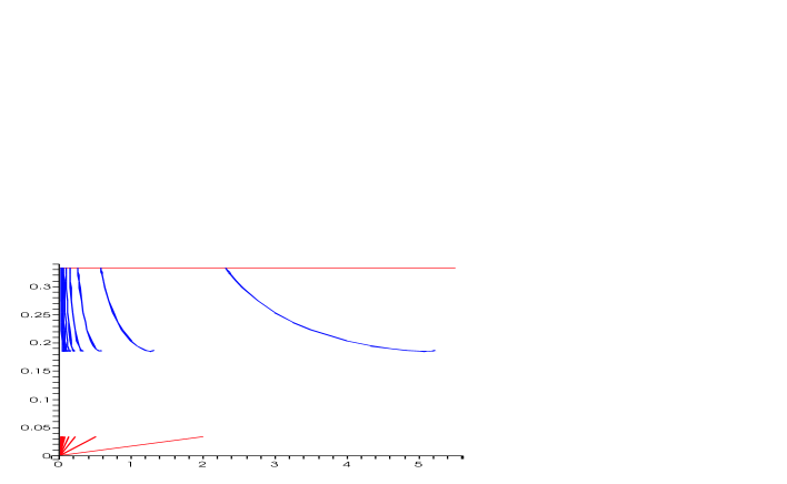
Figure 1: Phase diagram for $d=5$ in the region $n\leq 1/3$.

Thermodynamics

For a neutral Kaluza-Klein black hole with a single connected horizon, we can find the temperature $T$ and entropy $S$ directly from the metric. It is useful to define the rescaled temperature $\mathfrak{t}$ and entropy $\mathfrak{s}$ by

$$\mathfrak{t}=LT\ ,\ \ \mathfrak{s}=\frac{16\pi G_{\rm N}}{L^{d-1}}S\ .$$ (2.7)

In terms of these quantities, the Smarr formula for Kaluza-Klein black holes is given by [23, 15]

$$\mathfrak{t}\mathfrak{s}=\frac{d-2-n}{d-1}\mu\ .$$ (2.8)

The first law of thermodynamics is

$$\delta\mu=\mathfrak{t}\,\delta\mathfrak{s}\ .$$ (2.9)

Combining (2.8) and (2.9), we get the useful relation

$$\frac{\delta\log\mathfrak{s}}{\delta\log\mu}=\frac{d-1}{d-2-n}\ ,$$ (2.10)

so that, given a curve $n(\mu)$ in the phase diagram, the entire thermodynamics can be obtained.

As seen in [22], there are also neutral Kaluza-Klein black hole solution with more than one connected event horizon. The generalization of the Smarr formula (2.8) and first law (2.9) were found in [22] for the specific class of solutions considered there.

The ansatz

As mentioned above, the solutions with $0\leq n\leq 1/(d-2)$ have, to our present knowledge, a local $SO(d-1)$ symmetry. Using this symmetry it has been shown [44, 24] that the metric of these solutions can be written in the form

$$ds^{2}_{d+1}=-fdt^{2}+\frac{L^{2}}{(2\pi)^{2}}\left[\frac{A}{f}dR^{2}+\frac{A}{K^{d-2}}dv^{2}+KR^{2}d\Omega_{d-2}^{2}\right]\ ,\ \ f=1-\frac{R_{0}^{d-3}}{R^{d-3}}\ ,$$ (2.11)

where $R_{0}$ is a dimensionless parameter, $R$ and $v$ are dimensionless coordinates and the metric is determined by the two functions $A=A(R,v)$ and $K=K(R,v)$. The form (2.11) was originally proposed in Ref. [14] as an ansatz for the metric of black holes on cylinders.

The properties of the ansatz (2.11) were extensively considered in [14]. It was found that the function $A=A(R,v)$ can be written explicitly in terms of the function $K(R,v)$ thus reducing the number of free unknown functions to one. The functions $A(R,v)$ and $K(R,v)$ are periodic in $v$ with the period $2\pi$. Note that $R=R_{0}$ is the location of the horizon in (2.11).

The asymptotic region, i.e. the region far away from the black hole or string, is located at $R\rightarrow\infty$. We demand that $r/R\rightarrow L/(2\pi)$ and $z/v\rightarrow L/(2\pi)$ for $R\rightarrow\infty$. This is equivalent to demanding that $A,K\rightarrow 1$ for $R\rightarrow\infty$. Since $K(R,v)$ in principle determines the complete metric (2.11), we can read off the asymptotic quantities $\mu$ and $n$ from the first correction to $K(R,v)$. We define the parameter $\chi$ from $K(R,v)$ in the limit $R\rightarrow\infty$ by

$$K(R,v)=1-\chi\frac{R_{0}^{d-3}}{R^{d-3}}+\mathcal{O}(R^{-2(d-3)})\ .$$ (2.12)

Then, using (2.4), we can write the rescaled mass $\mu$ and relative tension $n$ in terms of $R_{0}$ and $\chi$ as

$$\mu=\frac{(d-3)\Omega_{d-2}}{(2\pi)^{d-3}}R_{0}^{d-3}\left[\frac{d-2}{d-3}-\chi\right]\ ,\ \ n=\frac{1-(d-2)(d-3)\chi}{d-2-(d-3)\chi}\ .$$ (2.13)

If we consider instead the solution near the horizon at $R=R_{0}$, we can read off the temperature and entropy in a precise manner. To this end, define

$$A_{h}\equiv A(R,v)|_{R=R_{0}}\ .$$ (2.14)

This is a meaningful definition since, as shown in [14], $A(R,v)$ is independent of $v$ on the horizon $R=R_{0}$. The thermodynamics [14, 23] is then

$$\mathfrak{t}=\frac{d-3}{2\sqrt{A_{h}}R_{0}}\ ,\ \ \mathfrak{s}=\frac{4\pi\Omega_{d-2}}{(2\pi)^{d-2}}\sqrt{A_{h}}R_{0}^{d-2}\ ,$$ (2.15)

in terms of the rescaled temperature and entropy defined in (2.7).

Copies

Finally, we note that for any solution in the ansatz (2.11) one can generate an infinite number of copies. This was found in [45, 24]. We refer to Ref. [24] for the transformation of the solution and mention here the relation between the physical quantities of the original solution and those of the copies

$$\mu^{\prime}=\frac{\mu}{k^{d-3}}\ ,\ \ n^{\prime}=n\ ,\ \ \mathfrak{t}^{\prime}=k\mathfrak{t}\ ,\ \ \mathfrak{s}^{\prime}=\frac{\mathfrak{s}}{k^{d-2}}\ ,$$ (2.16)

where $k$ is any positive integer. In Figure 1 we depicted the copies of the black hole on cylinder and non-uniform black string branches for $d=5$.

3 Defining a phase diagram for non-extremal branes on a circle

We define in this section what we precisely mean by a non-extremal brane on a circle. We define furthermore the asymptotic parameters that we use to categorize the solutions.

3.1 $1/2$ BPS branes of String/M-theory

Before defining more precisely the class of non-extremal branes that we consider, we begin by specifying what class of extremal branes they are thermal excitations of. As we explain in the following, the class of branes that we consider are thermal excitations of the $1/2$ BPS branes of Type IIA and IIB string theory and M-theory.

We consider singly-charged dilatonic $p$-branes in a $D$-dimensional space-time which are solutions to the equations of motion of the action

$$I_{D}=\frac{1}{16\pi G_{D}}\int d^{D}x\sqrt{-g}\left(R-\frac{1}{2}\partial_{\mu}\phi\partial^{\mu}\phi-\frac{1}{2(p+2)!}e^{a\phi}(F_{(p+2)})^{2}\right)\ ,$$ (3.1)

with $\phi$ the dilaton field and $F_{(p+2)}$ a $(p+2)$-form field strength with $F_{(p+2)}=dA_{(p+1)}$ where $A_{(p+1)}$ is the corresponding $(p+1)$-form gauge field. The action (3.1) is for $D=10$ the bosonic part of the low energy action of Type IIA and IIB string theory (in the Einstein-frame) when only one of the gauge-fields is present, and for $D=11$ it is the low energy action of M-theory, for suitable choices of $a$ and $p$. For use below we write the Einstein equations that follow from (3.1)

$$R_{\mu\nu}-\frac{1}{2}g_{\mu\nu}R=8\pi G_{D}T^{\rm mat}_{\mu\nu}=8\pi G_{D}(T^{\rm dil}_{\mu\nu}+T^{\rm el}_{\mu\nu})\ ,$$ (3.2)

$$\begin{array}[]{c}\displaystyle 8\pi G_{D}T^{\rm dil}_{\mu\nu}=-\frac{1}{4}g_{\mu\nu}\partial^{\rho}\phi\partial_{\rho}\phi+\frac{1}{2}\partial_{\mu}\phi\partial_{\nu}\phi\ ,\\ \displaystyle 8\pi G_{D}T^{\rm el}_{\mu\nu}=-\frac{1}{2}g_{\mu\nu}\frac{1}{2(p+2)!}e^{a\phi}(F_{(p+2)})^{2}+\frac{1}{2(p+1)!}e^{a\phi}F_{\mu}^{\ \rho_{1}\cdots\rho_{p+1}}F_{\nu\rho_{1}\cdots\rho_{p+1}}\ ,\end{array}$$ (3.3)

where $T^{\rm mat}_{\mu\nu}$ is the “matter” part of the action (3.1) consisting of the dilaton part $T^{\rm dil}_{\mu\nu}$ and the “electric” part $T^{\rm el}_{\mu\nu}$ due to the $(p+1)$-form gauge field .

We write in the following $d=D-p-1$ as the number of directions transverse to the $p$-brane.

The extremal $1/2$ BPS $p$-brane solutions in string theory and M-theory are then given by

$$ds^{2}=H^{-\frac{d-2}{D-2}}\left[-dt^{2}+\sum_{i=1}^{p}(du^{i})^{2}+Hds_{d}^{2}\right]\ ,$$ (3.4)

$$e^{2\phi}=H^{a}\ ,\ \ A_{(p+1)}=(H^{-1}-1)dt\wedge du^{1}\wedge\cdots\wedge du^{p}\ ,$$ (3.5)

with $\nabla^{2}H=0$ (away from the sources) where $ds_{d}^{2}$ is the (flat) metric and $\nabla^{2}$ the Laplacian for the $d$-dimensional transverse space. These solutions correspond to $1/2$ BPS extremal $p$-branes of String/M-theory when $D=10,11$ and

$$a^{2}=4-2\frac{(p+1)(d-2)}{D-2}\ .$$ (3.6)

Thus with (3.6) obeyed we get for $D=10$ the D-branes, NS5-brane and the F-string of Type IIA and IIB string theory, and for $D=11$ the M2-brane and M5-brane of M-theory. Note that the string theory solutions are written here in the Einstein frame.

We see that for the extremal solution (3.4)-(3.5) we can in particular consider the extremal $p$-branes to have $\mathbb{R}^{d-1}\times S^{1}$ as the transverse space. The thermal excitations of this class of extremal branes are precisely the non-extremal branes that we consider below.

3.2 Measuring asymptotic quantities

As mentioned above, the class of non-extremal branes we consider are thermal excitations of the extremal $1/2$ BPS branes in Type IIA/IIB String theory and M-theory with transverse space $\mathbb{R}^{d-1}\times S^{1}$. Therefore, since these non-extremal branes have a transverse circle we refer to them as non-extremal branes on a circle in this paper.

Clearly, for a given $p$-brane solution of this type we have that the solution asymptotes to $\mathcal{M}^{D-1}\times S^{1}=\mathcal{M}^{p+1}\times\mathbb{R}^{d-1}\times S^{1}$ far away from the brane, where the $p$-brane world-volume is along the $\mathcal{M}^{p+1}$ part. To be more specific, write the metric of $\mathcal{M}^{p+1}\times\mathbb{R}^{d-1}\times S^{1}$ as

$$ds^{2}=-dt^{2}+\sum_{i=1}^{p}(du^{i})^{2}+dr^{2}+r^{2}d\Omega_{d-2}^{2}+dz^{2}\ .$$ (3.7)

Here $t$ parameterizes the time, $u^{i}$, $i=1,..,p$, parameterize $\mathbb{R}^{p}$ (the spatial part of the world-volume), $r$ is the radius on $\mathbb{R}^{d-1}$ and $z$ is a periodic coordinate with period $L$ that parameterizes $S^{1}$. The $p$-brane metric thus asymptotes to the metric (3.7) far away from the brane.

In the discussion below it is useful, however, to consider each spatial world-volume direction $u^{i}$ of the $p$-brane to be compactified on a circle of length $L_{i}^{(u)}$. The solution then asymptotes to $\mathcal{M}^{d}\times\mathbb{T}^{p}\times S^{1}$ where $\mathbb{T}^{p}$ is a rectangular torus with volume $V_{p}=\prod_{i=1}^{p}L_{i}^{(u)}$.

For a given $p$-brane solution we consider the asymptotic region defined by $r\rightarrow\infty$. For $r\rightarrow\infty$ we have to leading order

$$g_{tt}\simeq-1+\frac{\bar{c}_{t}}{r^{d-3}}\ ,\ \ g_{zz}\simeq 1+\frac{\bar{c}_{z}}{r^{d-3}}\ ,\ \ g_{ii}\simeq 1+\frac{\bar{c}_{u}}{r^{d-3}}\ ,\ \ i=1\ldots p\ ,$$ (3.8)

for the metric and

$$A_{(p+1)}\simeq\frac{\bar{c}_{A}}{r^{d-3}}dt\wedge du^{1}\wedge\cdots\wedge du^{p}\ ,\ \ \phi\simeq\frac{\bar{c}_{\phi}}{r^{d-3}}\ ,$$ (3.9)

for the gauge field and dilaton. By writing the leading part of the gauge field $A_{(p+1)}$ as in (3.9) we have specified that it is only charged along the $p$-plane spanned by the $u^{1},...,u^{p}$ directions. We now explain how to measure the various asymptotic quantities in terms of $\bar{c}_{t}$, $\bar{c}_{z}$, $\bar{c}_{u}$, $\bar{c}_{A}$ and $\bar{c}_{\phi}$.

It is clear that we can use the general formulas of [25] (see also [46, 47]) to find the total mass $\bar{M}$, the total tension $\mathcal{T}_{i}^{(u)}$ along the $i$’th world-volume direction and the tension $\bar{\mathcal{T}}$ along the $z$-direction. This gives

$$\bar{M}=\frac{V_{p}L\Omega_{d-2}}{16\pi G_{D}}\left[(d-2)\bar{c}_{t}-\bar{c}_{z}-p\bar{c}_{u}\right]\ ,\ \ \bar{\mathcal{T}}=\frac{V_{p}\Omega_{d-2}}{16\pi G_{D}}\left[\bar{c}_{t}-(d-2)\bar{c}_{z}-p\bar{c}_{u}\right]\ ,$$ (3.10)

$$L_{i}^{(u)}\mathcal{T}_{i}^{(u)}=\frac{V_{p}L\Omega_{d-2}}{16\pi G_{D}}\left[\bar{c}_{t}-\bar{c}_{z}-(D-4)\bar{c}_{u}\right]\ .$$ (3.11)

Moreover, the charge $Q=\frac{V_{p}}{16\pi G_{D}}\int e^{a\phi}*\!F$ is measured to be

$$Q=\frac{V_{p}L\Omega_{d-2}}{16\pi G_{D}}(d-3)|\bar{c}_{A}|\ .$$ (3.12)

We can furthermore split up the mass in a gravitational, a dilatonic and an electric part as $\bar{M}=M^{\rm gr}+M^{\rm dil}+M^{\rm el}$, following (3.2)-(3.3). Similarly, we can split up the tension along the world-volume as $\mathcal{T}_{i}^{(u)}=(\mathcal{T}_{i}^{(u)})^{\rm gr}+(\mathcal{T}_{i}^{(u)})^{\rm dil}+(\mathcal{T}_{i}^{(u)})^{\rm el}$. We now explain how to measure $M^{\rm el}$ and $(\mathcal{T}_{i}^{(u)})^{\rm el}$.

It is useful in the following to apply the “principle of equivalent sources” and think of the total energy-momentum tensor $T_{\mu\nu}=T^{\rm gr}_{\mu\nu}+T^{\rm dil}_{\mu\nu}+T^{\rm el}_{\mu\nu}$ as the sum of a gravitational, a dilatonic and an electric part. Then we can write $M^{\rm gr}=\int T^{\rm gr}_{00}$, $M^{\rm dil}=\int T^{\rm dil}_{00}$ and $M^{\rm el}=\int T^{\rm el}_{00}$, and moreover $L_{i}^{(u)}(\mathcal{T}_{i}^{(u)})^{\rm gr}=-\int T^{\rm gr}_{ii}$, $L_{i}^{(u)}(\mathcal{T}_{i}^{(u)})^{\rm dil}=-\int T^{\rm dil}_{ii}$ and $L_{i}^{(u)}(\mathcal{T}_{i}^{(u)})^{\rm el}=-\int T^{\rm el}_{ii}$.

If we consider the electric part of the energy-momentum tensor $T^{\rm el}_{\mu\nu}$ in (3.3), we require boost invariance on the world-volume. This means that $T^{\rm el}_{00}=-T^{\rm el}_{ii}$ for all $i=1,...,p$. We see that this fixes

$$M^{\rm el}=L_{i}^{(u)}(\mathcal{T}_{i}^{(u)})^{\rm el}\ .$$ (3.13)

We require furthermore that the gravitational parts of the energy and tensions do not affect the world-volume directions, i.e. $\bar{c}^{\rm gr}_{u}=0$. Since from [25] we have that $\nabla^{2}g_{ii}=-16\pi G_{D}(T_{ii}-\frac{1}{D-2}T^{\rho}{}_{\rho})$ we see that this implies $T^{\rm gr}_{ii}=\frac{1}{D-2}(T^{\rm gr})^{\rho}{}_{\rho}$. Since furthermore one can see from (3.3) that $T^{\rm dil}_{ii}=\frac{1}{D-2}(T^{\rm dil})^{\rho}{}_{\rho}$, we have that $(T^{\rm gr}+T^{\rm dil})_{ii}=\frac{1}{D-2}(T^{\rm gr}+T^{\rm dil})^{\rho}{}_{\rho}$. This gives the condition

$$L_{i}^{(u)}(\mathcal{T}_{i}^{(u)}-(\mathcal{T}_{i}^{(u)})^{\rm el})=\frac{1}{d-1}(\bar{M}-M_{\rm el}+L\bar{\mathcal{T}})\ .$$ (3.14)

We get therefore

$$M_{\rm el}=\frac{1}{d-2}\left[(d-1)L_{i}^{(u)}\mathcal{T}_{i}^{(u)}-\bar{M}-\bar{\mathcal{T}}\right]\ ,$$ (3.15)

where $i$ can correspond to any of the world-volume directions. Using now (3.10)-(3.11) we get

$$M_{\rm el}=-\frac{V_{p}L\Omega_{d-2}}{16\pi G_{D}}\frac{(D-2)(d-3)}{d-2}\bar{c}_{u}\ .$$ (3.16)

It is important to note that, for the class of non-extremal $p$-branes that we consider here, $\bar{c}_{u}$ and $\bar{c}_{\phi}$ are not independent. We have the relation

$$\bar{c}_{u}=-\frac{d-2}{D-2}\frac{2\bar{c}_{\phi}}{a}\ ,$$ (3.17)

where $a$ is the constant defined in (3.1) determining the type of brane. This relation follows from the fact that we are looking at $p$-branes which are thermally excited supersymmetric $p$-branes, for which this relation applies.

The relation (3.17) is important for the D0-brane since $\bar{c}_{u}$ cannot be measured in that case. However, one can measure $\bar{c}_{\phi}$ and use (3.17) to find $\bar{c}_{u}$ and use this in the formulas (3.10)-(3.12).

Defining dimensionless quantities

Instead of using $\bar{M}$, $Q$, $\bar{\mathcal{T}}$ and $L_{i}^{(u)}\mathcal{T}_{i}^{(u)}$, it is useful to introduce the dimensionless quantities

$$\bar{\mu}=\frac{16\pi G_{D}}{V_{p}L^{d-2}}\bar{M}\ ,\ \ q=\frac{16\pi G_{D}}{V_{p}L^{d-2}}Q\ ,\ \ \bar{\mu}_{\rm el}=\frac{16\pi G_{D}}{V_{p}L^{d-2}}M^{\rm el}\ ,$$ (3.18)

$$\bar{n}=\frac{L\bar{\mathcal{T}}}{\bar{M}-M_{\rm el}}\ ,\ \ \bar{n}_{i}=\frac{L_{i}^{(u)}(\mathcal{T}_{i}^{(u)}-(\mathcal{T}_{i}^{(u)})^{\rm el})}{\bar{M}-M_{\rm el}}\ ,$$ (3.19)

where $\bar{\mu}$ is the rescaled mass, $q$ the rescaled charge, $\bar{n}$ the relative tension along the $z$-direction and $\bar{n}_{i}$ the relative tension along the $u^{i}$ world-volume direction.

We get from (3.10)-(3.12) the results

$$\bar{\mu}=\frac{\Omega_{d-2}}{L^{d-3}}\left[(d-2)\bar{c}_{t}-p\bar{c}_{u}-\bar{c}_{z}\right]\ ,\ \ q=\frac{\Omega_{d-2}}{L^{d-3}}(d-3)|\bar{c}_{A}|\ ,$$ (3.20)

$$\bar{n}=\frac{\bar{c}_{t}-(d-2)\bar{c}_{z}-p\bar{c}_{u}}{(d-2)\bar{c}_{t}-\bar{c}_{z}+\frac{d^{2}-4d-p+3}{d-2}\bar{c}_{u}}\ ,$$ (3.21)

which enable the determination of the three independent physical quantities $(\bar{\mu},\bar{n},q)$ from the asymptotics of the metric.

The relative tension $\bar{n}_{i}$ along each of the world-volume directions is

$$\bar{n}_{i}=\frac{1+\bar{n}}{d-1}\ ,\ \ i=1,\ldots,p\ .$$ (3.22)

Eq. (3.22) shows that the relative tension $\bar{n}_{i}$ is affected by the tension in the transverse direction. The physical reason is that extra tension is necessary in order to keep the $p$-brane directions flat while increasing the tension in the transverse direction. We also see from (3.22) that $\bar{n}=0$ correctly gives $\bar{n}_{i}=1/(d-1)$, reproducing the known result for $p$-branes [46]. On the other hand, substituting $\bar{n}=1/(d-2)$ gives $\bar{n}_{i}=1/(d-2)$, which is the correct result for a $(p+1)$-brane which is uniform in all directions. Note that from (3.13), (3.14) and the definitions (3.18), (3.19) it follows that the total dimensionless world-volume tension is

$$\tau_{(u)}\equiv\frac{16\pi G_{D}}{V_{p}L^{d-2}}L_{i}^{(u)}\mathcal{T}_{i}^{(u)}=\bar{n}_{i}(\bar{\mu}-\bar{\mu}_{\rm el})+\bar{\mu}_{\rm el}=\frac{1+\bar{n}}{d-1}\bar{\mu}+\frac{d-2-\bar{n}}{d-1}\bar{\mu}_{\rm el}\ ,$$ (3.23)

where we used the expression (3.22) for the relative tension $\bar{n}_{i}$ along the world-volume direction in terms of the relative tension in the transverse direction.

Bounds on $\bar{n}$

We examine now the general bounds [25]

$$\bar{M}\geq\frac{1}{D-3}\left(\sum_{i=1}^{p}L_{i}^{(u)}\mathcal{T}_{i}^{(u)}+L\bar{\mathcal{T}}\right)\ ,\ \ \mathcal{T}_{i}^{(u)}\geq 0\ ,\ \ \bar{\mathcal{T}}\geq 0\ ,$$ (3.24)

which we require to hold separately for all three contributions to the mass and tension. Firstly, for the electric contribution to the mass and tension it is easy to see that both bounds are trivially satisfied since $M_{\rm el}=L_{i}^{(u)}(\mathcal{T}_{i}^{(u)})^{\rm el}\geq 0$. If we consider (3.24) for the gravitational plus the dilatonic contributions together, these conditions are easily seen to be equivalent to the conditions

$$0\leq\bar{n}\leq d-2\ ,$$ (3.25)

using (3.19) and (3.22). The upper bound on $\bar{n}$ implies the bound $\tau_{(u)}\leq\bar{\mu}$ for the dimensionless world-volume tension.

Thermodynamics

It will also be useful to define, in analogy with (2.7), the dimensionless temperature and entropy for non-extremal branes

$$\bar{\mathfrak{t}}=L\bar{T}\ ,\ \ \bar{\mathfrak{s}}=\frac{16\pi G_{D}}{V_{p}L^{d-1}}\bar{S}\ ,$$ (3.26)

where $\bar{T}$ and $\bar{S}$ are the temperature and entropy of a non-extremal brane on a circle. Here we assume that we have only one connected event horizon. For more event horizons, one should consider more temperatures and entropies. The first law of thermodynamics, for constant charge $q$, takes the form

$$\delta\bar{\mu}=\bar{\mathfrak{t}}\,\delta\bar{\mathfrak{s}}\ .$$ (3.27)

The analogue of the neutral Smarr formula (2.8) follows easily from the general Smarr formula of [25] and the definitions (3.18), (3.19) and (3.26). The resulting non-extremal Smarr formula then takes the form

$$\bar{\mathfrak{t}}\bar{\mathfrak{s}}=\frac{d-2-\bar{n}}{d-1}\left(\bar{\mu}-\bar{\mu}_{\rm el}\right)\ ,$$ (3.28)

which is consistent with the bounds on $\bar{n}$ in (3.25).

World-volume tension is free energy

The dimensionless Helmholtz free energy is defined by

$$\bar{\mathfrak{f}}\equiv\bar{\mu}-\bar{\mathfrak{t}}\bar{\mathfrak{s}}\ .$$ (3.29)

Using the non-extremal Smarr formula (3.28) and comparing to (3.23) it immediately follows that

$$\tau_{(u)}=\bar{\mathfrak{f}}\ .$$ (3.30)

This shows that the world-volume tension is equal to the free energy for the general class of near-extremal brane that we have defined. Note in particular that this relation is a direct consequence of the physical properties that we have imposed on the branes.

Categorizing solutions

The program for non-extremal branes on a circle can now be formulated as taking any solution of the class defined above and reading off $\bar{\mu}$, $\bar{n}$ and $q$ using (3.20), (3.21). We can then consider all possible solutions for a given charge $q$ and draw a $(\bar{\mu},\bar{n})$ phase diagram depicting the values of $\bar{\mu}$ and $\bar{n}$ for all possible solutions. In this way we can categorize non-extremal branes on a circle in much the same way as for neutral and static Kaluza-Klein black holes.

Note that we can immediately dismiss certain values of $\bar{\mu}$ and $\bar{n}$ as being realized for physically viable solutions. We need clearly that $\bar{\mu}\geq q$ due to the fact that our non-extremal branes are thermal excitations of the supersymmetric branes with $\bar{\mu}=q$. Moreover, from (3.25) we have the bounds $0\leq\bar{n}\leq d-2$.

The question is now what one can say about the phase structure for a given charge $q$: How many solutions are known and how does the $(\bar{\mu},\bar{n})$ diagram look. In Section 4 we show that we can get at least part of the $(\bar{\mu},\bar{n})$ phase diagram by U-dualizing neutral and static Kaluza-Klein black holes.

4 Generating non-extremal branes

In this section we demonstrate that any static and neutral Kaluza-Klein black hole solution can be mapped to a solution for a non-extremal brane on a circle in Type IIA/B String theory and M-theory via U-duality. That one can “charge up” neutral solutions in this fashion was originally conceived in [49] where U-duality was used to obtain black $p$-branes from neutral black holes. Using this result we then prove that there is a map from the $(\mu,n)$ phase diagram for Kaluza-Klein black holes to the $(\bar{\mu},\bar{n})$ phase diagram for non-extremal branes on a circle. Finally, we show that one can use the map on the ansatz (2.11) to get an ansatz for certain phases of non-extremal branes on a circle.

4.1 Charging up solutions via U-duality

Consider a static and neutral Kaluza-Klein black hole solution, i.e. a static vacuum solution of $(d+1)$-dimensional General Relativity that asymptotes to $\mathcal{M}^{d}\times S^{1}$. We can always write the metric of such a solution in the form

$$ds^{2}_{d+1}=-Udt^{2}+\frac{L^{2}}{(2\pi)^{2}}V_{ab}dx^{a}dx^{b}\ ,$$ (4.1)

where $a,b=1,...,d$ and $V_{ab}$ is a symmetric tensor. Moreover, $U$ and $V_{ab}$ are functions of $x^{1},..,x^{d}$. In the asymptotic region we have that $U\rightarrow 1$ and $L^{2}(2\pi)^{-2}V_{ab}dx^{a}dx^{b}$ describes the cylinder $\mathbb{R}^{d-1}\times S^{1}$. The factor $L^{2}/(2\pi)^{2}$, where $L$ is the circumference of the circle in $\mathcal{M}^{d}\times S^{1}$, has been included in (4.1) for later convenience.

Using the $(d+1)$-dimensional metric we can construct the eleven-dimensional metric

$$ds^{2}_{11}=-Udt^{2}+\frac{L^{2}}{(2\pi)^{2}}V_{ab}dx^{a}dx^{b}+dy^{2}+\sum_{i=1}^{9-d}(du^{i})^{2}\ .$$ (4.2)

The metric (4.2) is clearly a vacuum solution of M-theory. Make now a Lorentz-boost along the $y$-axis so that

$$\left(\begin{array}[]{c}t_{\rm new}\\ y_{\rm new}\end{array}\right)=\left(\begin{array}[]{cc}\cosh\alpha&\sinh\alpha\\ \sinh\alpha&\cosh\alpha\end{array}\right)\left(\begin{array}[]{c}t_{\rm old}\\ y_{\rm old}\end{array}\right)\ .$$ (4.3)

This gives the boosted metric

$$ds^{2}_{11} = \left(-U\cosh^{2}\alpha+\sinh^{2}\alpha\right)dt^{2}+2(1-U)\cosh\alpha\sinh\alpha\,dtdy$$ (4.4)

$$+\left(-U\sinh^{2}\alpha+\cosh^{2}\alpha\right)dy^{2}+\frac{L^{2}}{(2\pi)^{2}}V_{ab}dx^{a}dx^{b}+\sum_{i=1}^{9-d}(du^{i})^{2}\ .$$

Since we have an isometry in the $y$-direction we can now make an S-duality in the $y$-direction to obtain a solution of type IIA string theory. This gives

$$ds^{2}=-H^{-\frac{1}{2}}Udt^{2}+H^{\frac{1}{2}}\left(\frac{L^{2}}{(2\pi)^{2}}V_{ab}dx^{a}dx^{b}+\sum_{i=1}^{9-d}(du^{i})^{2}\right)\ ,$$ (4.5)

$$H=1+\sinh^{2}\alpha\,(1-U)\ ,\ \ e^{2\phi}=H^{\frac{3}{2}}\ ,\ \ A=\coth\alpha\,(H^{-1}-1)dt\ .$$ (4.6)

This is a non-extremal D0-brane solution in type IIA string theory. For $d<9$ the D0-branes are uniformly smeared along an $\mathbb{R}^{9-d}$ space and they have transverse space $\mathbb{R}^{d-1}\times S^{1}$, i.e. they have a transverse circle. The solution (4.5)-(4.6) is written in the string-frame.

We can now use U-duality to transform the solution (4.5)-(4.6) into a D$p$-brane solution, an F-string solution or an NS5-brane solution of Type IIA/B String theory, or to an M2-brane or M5-brane solution of M-theory. In general, we U-dualize into the class of non-extremal branes on a circle defined in Section 3, which are non-extremal singly charged $p$-branes on a circle in $D$ dimensions with $D=d+p+1$ (for String/M-theory we have $D=10$/$D=11$). We can then write all these solutions as solutions to the EOMs of the action (3.1), as explained in Section 3.1. Thus, by U-duality we get

$$ds^{2}=H^{-\frac{d-2}{D-2}}\left(-Udt^{2}+\sum_{i=1}^{p}(du^{i})^{2}+\frac{L^{2}}{(2\pi)^{2}}H\,V_{ab}dx^{a}dx^{b}\right)\ ,$$ (4.7)

$$H=1+\sinh^{2}\alpha\,(1-U)\ ,$$ (4.8)

$$e^{2\phi}=H^{a}\ ,\ \ A_{(p+1)}=\coth\alpha\,(H^{-1}-1)dt\wedge du^{1}\wedge\cdots\wedge du^{p}\ .$$ (4.9)

This solution is a non-extremal $p$-brane with a transverse circle. It is written in the Einstein frame for the Type IIA/B String theory solutions.

In conclusion, we have shown by employing a boost and a U-duality transformation that we can transform any static and neutral Kaluza-Klein black hole solution (4.1) into the solution (4.7)-(4.9) describing non-extremal $p$-branes on a circle. This is one of the central results of this paper. Note that the transformation only works if $U$ is non-constant.

We also see that if we have an event horizon in the metric (4.1), $U\rightarrow 0$ near the event horizon. This translates into an event horizon in the non-extremal solution (4.7)-(4.9). Since the harmonic function (4.8) stays finite and non-zero for $U\rightarrow 0$, we see from this that the source for the electric potential $A_{(p+1)}$ in (4.9) is hidden behind the event horizon.

Finally, we note that if we have a number of event horizons defined by $U=0$, then from (4.9) we can measure the chemical potential $\nu$ to be

$$\nu=-A_{tu^{1}\cdots u^{p}}|_{U=0}=\tanh\alpha\ .$$ (4.10)

Thus, for the class of non-extremal solutions (4.7)-(4.9), obtained by a boost/U-duality transformation on neutral Kaluza-Klein black holes, we have that the chemical potential is given by (4.10). Therefore, even though we might have several disconnected event horizons, we have that $\nu=\tanh\alpha$ on all of them.

In the following we assume that we have at least one event horizon present.

4.2 Mapping of phase diagram

Given the above map from neutral Kaluza-Klein black holes to non-extremal branes on a circle, we now use the results of Section 3 to find the induced map for the physical quantities. Our goal in the following is: Given $\mu$ and $n$ for the Kaluza-Klein black hole, find $\bar{\mu}$ and $\bar{n}$ for the corresponding non-extremal brane on a circle for a given charge $q$.

We begin by expressing the leading-order behavior of the non-extremal solution (4.7)-(4.9) in terms of that of the neutral solution (4.1), for which we have the asymptotics (2.2). We have

$$U=-g_{tt}=1-\frac{c_{t}}{r^{d-3}}+\mathcal{O}(r^{-2(d-3)})\ ,$$ (4.11)

and hence

$$H=1+\frac{c_{t}\sinh^{2}\alpha}{r^{d-3}}+\mathcal{O}(r^{-2(d-3)})\ .$$ (4.12)

Moreover, for the spatial part $V_{ab}$ of the neutral metric, we only need that in spherically symmetric coordinates at infinity, $g_{zz}=1+c_{z}/r^{d-3}+\mathcal{O}(r^{-2(d-3)})$. Substituting this into (4.7)-(4.9) and comparing to (3.8), (3.9) then gives the relations

$$\bar{c}_{t}=c_{t}+\frac{d-2}{D-2}c_{t}\sinh^{2}\alpha\ ,\ \ \bar{c}_{z}=c_{z}+\frac{p+1}{D-2}c_{t}\sinh^{2}\alpha\ ,$$ (4.13)

$$\bar{c}_{u}=-\frac{d-2}{D-2}c_{t}\sinh^{2}\alpha\ ,\ \ |\bar{c}_{A}|=c_{t}\cosh\alpha\sinh\alpha\ ,$$ (4.14)

and $\bar{c}_{\phi}$ related to $\bar{c}_{u}$ by (3.17). Using these expressions in (3.18), (3.19) we can then write the three independent physical parameters $(\bar{\mu},\bar{n},q)$ of the non-extremal brane in terms of the boost parameter $\alpha$ and the two independent quantities $c_{t}$, $c_{z}$ of the neutral solution. Using (2.4), the latter two can be eliminated in favor of the physical parameters $(\mu,n)$ of the neutral solution, yielding the result

$$\bar{\mu}=\mu\left(1+\frac{d-2-n}{d-1}\sinh^{2}\alpha\right)\ ,\ \ q=\mu\frac{d-2-n}{d-1}\cosh\alpha\,\sinh\alpha\ ,\ \ \bar{n}=n\ .$$ (4.16)

We can now solve the second relation in (4.16) for $\alpha$,

$$\cosh\alpha(\mu,n,q)=\frac{1+b+\sqrt{1+b^{2}}}{2\sqrt{b(1+\sqrt{1+b^{2}})}}\ ,\ \ b\equiv\frac{d-2-n}{2(d-1)}\frac{\mu}{q}\ .$$ (4.17)

Substituting Eq. (4.17) in Eqs. (4.16) we obtain the map

$$\bar{\mu}=q+\frac{(d+n)}{2(d-1)}\mu+\frac{\left(\frac{d-2-n}{2(d-1)}\right)^{2}\frac{\mu^{2}}{q}}{1+\sqrt{1+\left(\frac{(d-2-n)\mu}{2(d-1)q}\right)^{2}}}\ ,\ \ \bar{n}=n\ .$$ (4.18)

Thus, given a neutral Kaluza-Klein black hole with mass $\mu$ and relative tension $n$, the transformation (4.18) gives us the mass $\bar{\mu}$ and relative tension $\bar{n}$ for the corresponding non-extremal $p$-brane on a circle for a given charge $q$. Note that we can also write $\bar{\mu}=\mu+\nu(\mu,n,q)q$ where $\nu(\mu,n,q)=\tanh\alpha(\mu,n,q)$.

As a consequence of the map (4.18) we see that from knowing the phase structure of the $(\mu,n)$ phase diagram for neutral Kaluza-Klein black holes we get at least part of the phase structure of the $(\bar{\mu},\bar{n})$ phase diagram for non-extremal branes on a circle.

Mapping of thermodynamics

If we assume that the neutral Kaluza-Klein black hole with metric (4.1) has a single connected event horizon defined by $U=0$, we can measure the (rescaled) temperature $\mathfrak{t}$ and entropy $\mathfrak{s}$. For the corresponding solution of non-extremal branes on a circle (4.7)-(4.9) we can then read off the (rescaled) temperature $\bar{\mathfrak{t}}$ and entropy $\bar{\mathfrak{s}}$. By using that $H=\coth^{2}\alpha$ on the horizon, it is then easily seen that we get the map

$$\bar{\mathfrak{t}}\bar{\mathfrak{s}}=\mathfrak{t}\mathfrak{s}\ ,\ \ \bar{\mathfrak{t}}\cosh\alpha=\mathfrak{t}\ ,$$ (4.19)

where $\alpha$ is given in (4.17) in terms of $\mu$, $n$ and $q$.

Tension on world-volume

For use below we also give the expression of the tension in the spatial world-volume of the brane

$$\tau_{(u)}=\mu\left(\frac{1+n}{d-1}+\frac{d-2-n}{d-1}\sinh^{2}\alpha\right)\ ,$$ (4.20)

which follows from (3.23) and (4.16). Using (4.17) to eliminate $\alpha$, we get

$$\tau_{(u)}=q+\frac{(4-d+3n)}{2(d-1)}\mu+\frac{\left(\frac{d-2-n}{2(d-1)}\right)^{2}\frac{\mu^{2}}{q}}{1+\sqrt{1+\left(\frac{(d-2-n)\mu}{2(d-1)q}\right)^{2}}}\ ,$$ (4.21)

which shows a similar structure as the mass $\bar{\mu}$ in (4.18).

4.3 Ansatz for non-extremal branes on a circle

As reviewed in Section 2 we can write all Kaluza-Klein black hole solutions with a local $SO(d-1)$ symmetry, which seems to apply to all solutions with $n\leq 1/(d-2)$, with the metric in the form of the ansatz (2.11). Now, using this $(d+1)$-dimensional metric (2.11) we can apply the same boost/U-duality transformation as for the general metric (4.1). Using (4.7)-(4.9) we get the following $p$-brane solution in $D=d+p+1$ dimensions

$$ds^{2}=H^{-\frac{d-2}{D-2}}\left(-fdt^{2}+\sum_{i=1}^{p}(du^{i})^{2}+H\frac{L^{2}}{(2\pi)^{2}}\left[\frac{A}{f}dR^{2}+\frac{A}{K^{d-2}}dv^{2}+KR^{2}d\Omega_{d-2}^{2}\right]\right)\ ,$$ (4.22)

$$e^{2\phi}=H^{a}\ ,\ \ A_{(p+1)}=\coth\alpha\,(H^{-1}-1)dt\wedge du^{1}\wedge\cdots\wedge du^{p}\ ,$$ (4.23)

$$f=1-\frac{R_{0}^{d-3}}{R^{d-3}}\ ,\ \ H=1+\sinh^{2}\alpha\frac{R_{0}^{d-3}}{R^{d-3}}\ .$$ (4.24)

This solution describes non-extremal $p$-branes on a circle. It is written in the Einstein frame for the Type IIA/B String theory solutions.

It is interesting to notice that this correspondence was already discovered in Ref. [14]. In Ref. [14] it was shown at the level of equations of motion that for any solution that can be written in the ansatz (2.11) a corresponding non-extremal $p$-brane solution of string theory or M-theory could be obtained. The above boost/U-duality derivation thus provides us with a physical understanding of this correspondence.

Regarding the topology of the horizon for the non-extremal solution (4.22)-(4.24) we note that if the neutral solution (2.11) is a black hole (black string) on a cylinder it has horizon topology $S^{d-1}$ ($S^{d-2}\times S^{1}$) and then the topology of the horizon in the non-extremal $p$-brane solution (4.22)-(4.24) is $\mathbb{R}^{p}\times S^{d-1}$ ($\mathbb{R}^{p}\times S^{d-2}\times S^{1}$).

The dimensionless physical quantities $\bar{\mu}$, $\bar{n}$, $\bar{\mathfrak{t}}$, $\bar{\mathfrak{s}}$, $\nu$ and $q$ can now be found directly for a given solution in the ansatz (4.22)-(4.24). Defining $\chi$ and $A_{h}$ as in (2.12) and (2.14), we find [14]

$$\bar{\mu}=\frac{(d-3)\Omega_{d-2}}{(2\pi)^{d-3}}R_{0}^{d-3}\left[\frac{d-2}{d-3}-\chi+\sinh^{2}\alpha\right]\ ,\ \ \bar{n}=\frac{1-(d-2)(d-3)\chi}{d-2-(d-3)\chi}\ ,$$ (4.25)

$$\bar{\mathfrak{t}}=\frac{d-3}{2\sqrt{A_{h}}R_{0}\cosh\alpha}\ ,\ \ \bar{\mathfrak{s}}=\frac{4\pi\Omega_{d-2}}{(2\pi)^{d-2}}\sqrt{A_{h}}R_{0}^{d-2}\cosh\alpha\ ,$$ (4.26)

$$\nu=\tanh\alpha\ ,\ \ q=\frac{(d-3)\Omega_{d-2}}{(2\pi)^{d-3}}R_{0}^{d-3}\cosh\alpha\,\sinh\alpha\ .$$ (4.27)

It is easy to see that Eqs. (4.25)-(4.27) are consistent with the transformation rules (4.16) and (4.19) using the thermodynamics (2.13), (2.15) for the ansatz (2.11) for Kaluza-Klein black holes.

As stated in Section 2 we have three phases of Kaluza-Klein black holes with local $SO(d-1)$ symmetry: The uniform black string, the non-uniform black string and the black hole on cylinder branch. Via the map of Section 4.1, all these branches generate a non-extremal solutions that fit into the ansatz (4.22)-(4.24).

We treat the non-extremal branch generated from the black hole on cylinder in Section 8 (the localized phase) and the non-extremal branch generated from the non-uniform black string in Section 9 (the non-uniform phase). The non-extremal branch generated from the uniform black string branch is treated below.

The uniform phase: Non-extremal branes smeared on a circle

We use here the boost/U-duality map discussed above on the uniform black string branch. This generates non-extremal branes smeared on a circle. We refer to this as the uniform phase of non-extremal branes on a circle.

The uniform black string branch is obtained in the ansatz (2.11) by putting $A(R,v)=K(R,v)=1$. Therefore, we obtain the solution for non-extremal branes smeared on a circle by setting $A(R,v)=K(R,v)=1$ in Eqs. (4.22)-(4.24), yielding

$$ds^{2}=H^{-\frac{d-2}{D-2}}\left(-fdt^{2}+\sum_{i=1}^{p}(du^{i})^{2}+H\frac{L^{2}}{(2\pi)^{2}}\left[\frac{1}{f}dR^{2}+dv^{2}+R^{2}d\Omega_{d-2}^{2}\right]\right)\ ,$$ (4.28)

$$e^{2\phi}=H^{a}\ ,\ \ A_{(p+1)}=\coth\alpha\,(H^{-1}-1)dt\wedge du^{1}\wedge\cdots\wedge du^{p}\ ,$$ (4.29)

$$f=1-\frac{R_{0}^{d-3}}{R^{d-3}}\ ,\ \ H=1+\sinh^{2}\alpha\frac{R_{0}^{d-3}}{R^{d-3}}\ .$$ (4.30)

This solution is well known, but we write it here explicitly for the sake of clarity. Note that comparing with (3.7) for $R\rightarrow\infty$ we see that $R=2\pi r/L$ and $v=2\pi z/L$. The physical quantities for this solution can easily be found by setting $\chi=0$ and $A_{h}=1$ in Eqs. (4.25)-(4.27).

5 Defining a phase diagram for near-extremal branes on a circle

In Section 3 we defined the class of non-extremal $p$-branes that we consider in the main part of this paper to be thermally excited states of the $1/2$ BPS branes of String and M-theory. In this class of branes, we can define a near-extremal brane to be a non-extremal brane with infinitesimally small temperature, or, equivalently, a non-extremal brane with infinitely high charge. As we shall see in Section 6, it is possible for any of the phases of non-extremal branes on a circle obtained from the map of Section 4.1 to take a near-extremal limit and obtain a corresponding phase of a near-extremal brane on a circle. Therefore, we define in this section what we mean by a near-extremal brane on a circle and how to measure the energy and tension for such a brane. This defines a new two-dimensional phase diagram for near-extremal branes on a circle, analogous to the two-dimensional $(\mu,n)$ phase diagram for static and neutral Kaluza-Klein black holes.

Near-extremal branes on a circle

Consider a given non-extremal $p$-brane on a circle, as defined in Section 3. We can write the metric as

$$ds^{2}=C^{(f)}\bigg{(}-C^{(t)}dt^{2}+\sum_{i=1}^{p}(du^{i})^{2}+\sum_{a,b=1}^{d}C^{(x)}_{ab}dx^{a}dx^{b}\bigg{)}\ ,$$ (5.1)

where $t$ is the time-direction, $u^{i}$ the spatial world-volume directions, $x^{a}$ the transverse directions parameterizing $\mathbb{R}^{d-1}\times S^{1}$ in the asymptotic region, and $C^{(f)}$, $C^{(t)}$, $C^{(x)}_{ab}$ are functions of $x^{1},...,x^{d}$. For such a solution, we want to take a near-extremal limit such that the size of the circle has the same scale as the excitations of the energy above extremality. This is because we want to keep the non-trivial physics related to the presence of the circle. Therefore, for a non-extremal $p$-brane with volume $V_{p}$, circumference $L$ and rescaled charge $q$, the near-extremal limit is

$$q\rightarrow\infty\ ,\ \ L\rightarrow 0\ ,\ \ g\equiv\frac{16\pi G_{D}}{V_{p}L^{d-2}}\ \,\mbox{fixed }\ ,\ \ l\equiv L\sqrt{q}\ \,\mbox{fixed }\ ,\ \ x^{a}\ \,\mbox{fixed }\ .$$ (5.2)

Note that in the metric (5.1) we keep $C^{(t)}(x^{1},...,x^{d})$ and $C^{(x)}_{ab}(x^{1},...,x^{d})$ fixed in the near-extremal limit (5.2). As we shall see below, the near-extremal limit (5.2) is defined so that the energy above extremality $\bar{\mu}-q$ is finite.

In the near-extremal limit (5.2) we rescale the metric in the transverse directions $x^{a}$. Given a non-extremal brane, this means that after the near-extremal limit the asymptotics of the solution has changed, and we find below how the asymptotic region looks for near-extremal branes on a circle. For the non-extremal branes we use the asymptotic coordinate system (3.7). Therefore, following (5.1) and (5.2), we should rescale $\hat{r}=2\pi r/L$ and $\hat{z}=2\pi z/L$. From this we see that the circumference of the circle transverse to the branes has the length $2\pi$. We also see that the asymptotic region for the near-extremal branes is $\hat{r}\rightarrow\infty$.

To understand better the near-extremal limit (5.2) it is important to consider this limit taken on an extremal brane on a circle, both since that can tell us about the asymptotic region $\hat{r}\rightarrow\infty$ of general near-extremal branes on a circle and also since it will be the reference space when measuring asymptotic physical quantities, as we shall see below.

The solution of extremal branes on a circle is given in Eqs. (3.4)-(3.5). Taking the near-extremal limit (5.2) of this solution, we get

$$ds^{2}=\hat{H}^{-\frac{d-2}{D-2}}\left(-dt^{2}+\sum_{i=1}^{p}(du^{i})^{2}+\hat{H}\left[d\hat{r}^{2}+\hat{r}^{2}d\Omega_{d-2}^{2}+d\hat{z}^{2}\right]\right)\ ,$$ (5.3)

$$e^{2\phi}=\hat{H}^{a}\ ,\ \ A_{(p+1)}=\hat{H}^{-1}dt\wedge du^{1}\wedge\cdots\wedge du^{p}\ ,$$ (5.4)

$$\hat{H}=\frac{\hat{h}_{d}}{\hat{r}^{d-3}}\ ,\ \ \hat{h}_{d}\equiv\frac{l^{2}(2\pi)^{d-5}}{(d-3)\Omega_{d-2}}\ ,$$ (5.5)

for $\hat{r}\rightarrow\infty$. Note that we defined $\hat{H}=HL^{2}/(2\pi)^{2}$ and that the solution is written in units of $L/(2\pi)$, which means that we have rescaled the fields with powers of $L/(2\pi)$. The solution (5.3)-(5.5) is exact for an extremal brane smeared uniformly on the circle, while there are for example corrections for an extremal brane localized at one point of the circle. In general all extremal branes localized in a point of the $\mathbb{R}^{d-1}$ of the cylinder $\mathbb{R}^{d-1}\times S^{1}$ are described by the solution (5.3)-(5.4) with

$$\hat{H}=\frac{\hat{h}_{d}}{\hat{r}^{d-3}}\left(1+\mathcal{O}(e^{-\hat{r}})\right)\ ,$$ (5.6)

for $\hat{r}\rightarrow\infty$. Thus, the first correction to the solution (5.3)-(5.5) comes in at order $e^{-\hat{r}}$. This will be important below since we use the extremal solution as the reference space for measuring asymptotic physical quantities.

If we consider now a near-extremal brane on a circle, we have that in the asymptotic region $\hat{r}\rightarrow\infty$, the solution asymptotes to that given by Eqs. (5.3)-(5.5), for a given value of $l$. We clearly see that the near-extremal solutions asymptote to a non-flat space-time described by the metric (5.3). As opposed to the extremal case, the first correction for a near-extremal brane on a circle to the solution given by Eqs. (5.3)-(5.5) will in general appear at order $\hat{r}^{-(d-3)}$ relative to the leading order solution.

Measuring energy and tension

Let a near-extremal brane on a circle be given. We can then define asymptotic physical quantities by comparing the solution to the extremal reference background given by Eqs. (5.3)-(5.4) and (5.6). Using the definition of energy in [40] and the definition of tension in [25] we have that the energy $E$, the tension $\hat{\mathcal{T}}$ along $z$ and the tension $\hat{\mathcal{T}}_{i}^{(u)}$ in a world-volume direction $u^{i}$, are given by

$$E=-\frac{2}{(2\pi)^{d-2}gV_{p}}\int_{S^{\infty}_{t}}N_{t}\left({\cal{K}}^{(D-2)}-{\cal{K}}_{0}^{(D-2)}\right)\ ,$$ (5.7)

$$\hat{\mathcal{T}}=-\frac{2}{(2\pi)^{d-2}gV_{p}}\int_{\hat{S}^{\infty}_{z}}N_{z}\left({\cal{K}}^{(D-2)}-{\cal{K}}_{0}^{(D-2)}\right)\ ,$$ (5.8)

$$\hat{\mathcal{T}}_{i}^{(u)}=-\frac{2}{(2\pi)^{d-2}gV_{p}}\int_{\hat{S}^{\infty}_{u}}N_{u}\left({\cal{K}}^{(D-2)}-{\cal{K}}_{0}^{(D-2)}\right)\ .$$ (5.9)

Here $N_{t}$, $N_{z}$ and $N_{u}$ are the lapse functions in the $t$, $z$ and $u^{i}$ directions, respectively. $S^{\infty}_{t}$ is a $(D-2)$-dimensional surface at infinity (i.e. with $\hat{r}\rightarrow\infty$) transverse to the $t$-direction. $\hat{S}^{\infty}_{z}$ and $\hat{S}^{\infty}_{u}$ are instead $(D-3)$-dimensional surfaces transverse to the $z$ and $u^{i}$ directions, respectively, and both transverse to the $t$-direction since we do not want to integrate over the time-direction. Moreover, ${\cal{K}}^{(D-2)}$ is the extrinsic curvature of the near-extremal brane solution while ${\cal{K}}_{0}^{(D-2)}$ is the extrinsic curvature of the reference space, which is the extremal brane solution given by (5.3)-(5.4) and (5.6). In Appendix A we compute $E$, $\hat{\mathcal{T}}$ and $\hat{\mathcal{T}}_{i}^{(u)}$ using Eqs. (5.7)-(5.9) for a particular class of solutions.

We define now the rescaled energy $\epsilon$, the relative tension $r$ and the relative world-volume tension $r_{u}$ as

$$\epsilon=gE\ ,\ \ r=\frac{2\pi\hat{\mathcal{T}}}{E}\ ,\ \ r_{u}=\frac{L_{i}^{(u)}\hat{\mathcal{T}}_{i}^{(u)}}{E}\ .$$ (5.10)

These quantities are useful since they are dimensionless.

Given any near-extremal brane on a circle, we can read off the two quantities $(\epsilon,r)$. Therefore, we can make an $(\epsilon,r)$ phase diagram for all the near-extremal brane on a circle. The program for near-extremal branes on a circle can now be formulated as taking any solution of the class defined above, and depicting the corresponding values for $\epsilon$ and $r$ in a $(\epsilon,r)$ phase diagram for all possible solutions. This is analogous to the $(\mu,n)$ phase diagram for neutral and static Kaluza-Klein black holes reviewed in Section 2.

In Sections 6-9 we show that many of the features of the $(\mu,n)$ phase diagram for neutral and static Kaluza-Klein black holes are carried over to the near-extremal branes on a circle. In particular, we show in Section 6 that we have a map that gives a near-extremal brane on a circle from a neutral and static Kaluza-Klein black hole solution.

For a given near-extremal brane on a circle with a single connected horizon we can also read off the temperature $\hat{T}$ and entropy $\hat{S}$. It is useful to define the dimensionless versions of the temperature and entropy

$$\hat{\mathfrak{t}}=l\,\hat{T}\ ,\ \ \hat{\mathfrak{s}}=\frac{g}{l}\hat{S}\ ,$$ (5.11)

since $l$ and $g$ in (5.2) have dimension length. The first law of thermodynamics for near-extremal branes then takes the form

$$\delta\epsilon=\hat{\mathfrak{t}}\,\delta\hat{\mathfrak{s}}\ .$$ (5.12)

Finally, we note that one can get the physical quantities for the near-extremal brane directly from the physical quantities of the non-extremal brane in the near-extremal limit (5.2). We have

$$E=\lim_{L\rightarrow 0}\left(\bar{M}-Q\right)\ ,\ \ \hat{\mathcal{T}}=\lim_{L\rightarrow 0}\frac{L}{2\pi}\bar{\mathcal{T}}\ ,\ \ L_{i}^{(u)}\hat{\mathcal{T}}_{i}^{(u)}=\lim_{L\rightarrow 0}\left(L_{i}^{(u)}\mathcal{T}_{i}^{(u)}-Q\right)\ ,$$ (5.13)

$$\hat{T}=\lim_{L\rightarrow 0}\bar{T}\ ,\ \ \hat{S}=\lim_{L\rightarrow 0}\bar{S}\ .$$ (5.14)

We only prove the validity of these relations for a special class of solutions in this paper, namely for the near-extremal limit of the non-extremal branes on a circle that can be written in the ansatz (4.22)-(4.24). However, from a physical perspective, these relations are expected to hold for the complete class of non-extremal branes on a circle in the near-extremal limit (5.2).

Note that as a consequence of the first relation in (5.13) we have that

$$\epsilon=\lim_{L\rightarrow 0}(\bar{\mu}-q)\ .$$ (5.15)

It follows from this that the energy above extremality $\bar{\mu}-q$ is finite in the near-extremal limit.

6 Generating near-extremal branes

We constructed in Section 4 a map that takes a given neutral and static Kaluza-Klein black hole and transforms it into a solution for non-extremal branes on a circle, using a boost/U-duality transformation. In this section, we take the near-extremal limit of this map and thereby obtain a map that instead takes a given Kaluza-Klein black hole solution to a solution for near-extremal branes on a circle. This in turn induces a map from the $(\mu,n)$ phase diagram for Kaluza-Klein black holes to the $(\epsilon,r)$ phase diagram for near-extremal branes on a circle. Finally, we show that one can use the map on the ansatz (2.11) to get an ansatz for certain phases of near-extremal branes on a circle.

6.1 Near-extremal limit of U-dual brane solution

Let a static and neutral Kaluza-Klein black hole be given. The metric can be written in the form (4.1). In Section 4 we learned that we can transform the Kaluza-Klein black hole into the solution (4.7)-(4.9) describing non-extremal $p$-branes on a circle. We now take the near-extremal limit (5.2) of (4.7)-(4.9). Note first that we need to write $U$ and $V_{ab}$ as functions of the dimensionless variables $x^{1},...,x^{d}$. In this way $U$ and $V_{ab}$ do not change under the near-horizon limit (5.2). Note also that $\hat{r}=2\pi r/L$ and $\hat{z}=2\pi z/L$ can be used as two of these dimensionless variables. Then, from (2.2) we see that

$$U=1-\frac{\hat{c}_{t}}{\hat{r}^{d-3}}+\mathcal{O}(\hat{r}^{-2(d-3)})\ ,\ \ \hat{c}_{t}\equiv c_{t}\frac{L^{d-3}}{(2\pi)^{d-3}}\ ,$$ (6.1)

for $\hat{r}\rightarrow\infty$. Using now (3.20) and (4.14) we get that the charge $q$ can be written

$$q=\frac{(d-3)\Omega_{d-2}}{(2\pi)^{d-3}}\hat{c}_{t}\cosh\alpha\sinh\alpha\ .$$ (6.2)

Since $L\sqrt{q}$ should be fixed in the limit $L\rightarrow 0$ we see that $\alpha\rightarrow\infty$ with $Le^{\alpha}$ being fixed. Define the rescaled harmonic function

$$\hat{H}\equiv\lim_{L\rightarrow 0}\frac{L^{2}}{(2\pi)^{2}}H\ .$$ (6.3)

One can check that $\hat{H}$ is finite in the near-extremal limit (5.2). We can then write the resulting solution for near-extremal $p$-branes on a circle as

$$ds^{2}=\hat{H}^{-\frac{d-2}{D-2}}\left(-Udt^{2}+\sum_{i=1}^{p}(du^{i})^{2}+\hat{H}V_{ab}dx^{a}dx^{b}\right)\ ,$$ (6.4)

$$e^{2\phi}=\hat{H}^{a}\ ,\ \ A_{(p+1)}=\hat{H}^{-1}dt\wedge du^{1}\wedge\cdots\wedge du^{p}\ ,$$ (6.5)

where

$$\hat{H}=\hat{h}_{d}\frac{1-U}{\hat{c}_{t}}\ ,\ \ \hat{h}_{d}\equiv\frac{l^{2}(2\pi)^{d-5}}{(d-3)\Omega_{d-2}}\ .$$ (6.6)

Here the fields in (6.4)-(6.5) have been written in units of $L/(2\pi)$, i.e. we have rescaled the fields with the appropriate powers of $L/(2\pi)$ to get a finite solution.

It is important to note that, using (6.1) and (6.6), we have to leading order for $\hat{r}\rightarrow\infty$

$$\hat{H}=\frac{\hat{h}_{d}}{\hat{r}^{d-3}}+\mathcal{O}(\hat{r}^{-2(d-3)})\ ,$$ (6.7)

which agrees with the leading order harmonic function of the near-horizon limit of the extremal case, as given in (5.3)-(5.5). As a consequence, the near-extremal $p$-brane solutions generated this way correctly asymptote to the near-extremal limit of the extremal $p$-brane on a transverse circle, which is taken as the reference space when calculating energy and tensions.

In conclusion, we have that for any neutral Kaluza-Klein black hole with metric (4.1) we get the solution (6.4)-(6.6) describing near-extremal $p$-branes on a circle. This is one of the central results of this paper since it enables us to find new phases of near-extremal branes on a circle from the known phases of neutral Kaluza-Klein black holes. In particular, in the following we study the near-extremal $p$-brane solutions that follow from the black hole on cylinder branch and the non-uniform black string branch. The resulting solutions are respectively the phase for near-extremal branes localized on the circle (see Section 8) and a new non-uniform phase for near-extremal branes (see Section 9).

6.2 Mapping of phase diagram

We have shown above that any neutral Kaluza-Klein black hole can be mapped into a solution for near-extremal branes on a circle. As a consequence of this, we show in this section that we can map the physical parameters $\mu$ and $n$ for the neutral Kaluza-Klein black hole into $\epsilon$ and $r$ for the near-extremal branes on a circle. We furthermore find a map for the thermodynamics.

To find this map, we first note that we can easily read off what $\epsilon=\bar{\mu}-q$ becomes in terms of $\mu$ and $n$ using (4.18), since $q\rightarrow\infty$ in the near-extremal limit (5.2). For the tension, on the other hand, we can use that it follows from (3.10), (4.13) and (4.14) that

$$\bar{\mathcal{T}}=\frac{V_{p}\Omega_{d-2}}{16\pi G_{D}}\left[c_{t}-(d-2)c_{z}\right]\ ,$$ (6.8)

for non-extremal branes on a circle related to neutral Kaluza-Klein black holes by the map in Section 4.1. Then, using the near-extremal limit (5.2) and (5.13) we get

$$\hat{\mathcal{T}}=\frac{\mu n}{2\pi g}\ .$$ (6.9)

Collecting the above observations, we see that given a neutral Kaluza-Klein black hole with mass $\mu$ and relative tension $n$ we find that the corresponding near-extremal $p$-brane on a circle ($D=d+p+1$) has energy $\epsilon$ and relative tension $r$ given by

$$\epsilon=\frac{d+n}{2(d-1)}\mu\ ,\ \ r=2\frac{(d-1)n}{d+n}\ .$$ (6.10)

We remind the reader that the energy $\epsilon$ and relative tension $r$ are defined in (5.10).

The near-extremal map (6.10) is another of the central results of this paper since it gives a direct way to get the near-extremal $(\epsilon,r)$ phase diagram from the $(\mu,n)$ phase diagram for neutral Kaluza-Klein black holes.

For a solution with a single connected event horizon (defined by $U=0$) we have furthermore, that for a neutral Kaluza-Klein black hole with (rescaled) temperature $\mathfrak{t}$ and entropy $\mathfrak{s}$ the corresponding near-extremal brane on a circle has the (rescaled) temperature $\hat{\mathfrak{t}}$ and entropy $\hat{\mathfrak{s}}$ given by

$$\hat{\mathfrak{t}}\hat{\mathfrak{s}}=\mathfrak{t}\mathfrak{s}\ ,\ \ \hat{\mathfrak{t}}=\mathfrak{t}\sqrt{\mathfrak{t}\mathfrak{s}}\ .$$ (6.11)

To show this, one first finds that $\hat{\mathfrak{t}}=\bar{\mathfrak{t}}\sqrt{q}$ and $\hat{\mathfrak{s}}=\bar{\mathfrak{s}}/\sqrt{q}$ using (3.26), (5.2), (5.11) and (5.14). Then one finds from (4.16) and (2.8) that $q/\cosh^{2}\alpha\rightarrow\mathfrak{t}\mathfrak{s}$ in the near-extremal limit (5.2). Using this together with (4.19), one derives the map (6.11).

World-volume tension

Besides the mapping (6.10), it is also interesting to compute the near-extremal limit (5.2) of the expression (4.21) for the world-volume tension of non-extremal branes. In terms of the relative world-volume tension $r_{u}$ defined in (5.10) we find that

$$r_{u}=\frac{4-d+3n}{d+n}\ .$$ (6.12)

This is not an independent quantity for the near-extremal brane, since $r_{u}$ is related to relative tension in the transverse direction via

$$r_{u}=\frac{4-d+2r}{d}\ ,$$ (6.13)

which follows using (6.10) in (6.12). This relation is the analogue of (3.22) for non-extremal branes, which physically expresses the fact that the gravitational part of energy and tension does not affect the world-volume directions (see Section 3.2). Note that while the relation (3.22) follows in full generality from our definition of non-extremal branes on a circle, the relation (6.13) is proven here only for the class of near-extremal branes obtained in Section 6.1 via U-duality and the near-extremal limit.

6.3 Ansatz for near-extremal branes on a circle

For the neutral Kaluza-Klein black holes with local $SO(d-1)$ symmetry we can write the metric in the ansatz (2.11), as reviewed in Section 2. We can therefore use the map (6.4)-(6.6) to near-extremal $p$-branes on a circle. The resulting near-extremal $p$-brane solution is ($D=d+p+1$)

$$ds^{2}=\hat{H}^{-\frac{d-2}{D-2}}\left(-fdt^{2}+\sum_{i=1}^{p}(du^{i})^{2}+\hat{H}\left[\frac{A}{f}dR^{2}+\frac{A}{K^{d-2}}dv^{2}+KR^{2}d\Omega_{d-2}^{2}\right]\right)\ ,$$ (6.14)

$$e^{2\phi}=\hat{H}^{a}\ ,\ \ A_{(p+1)}=\hat{H}^{-1}dt\wedge du^{1}\wedge\cdots\wedge du^{p}\ ,$$ (6.15)

$$f=1-\frac{R_{0}^{d-3}}{R^{d-3}}\ ,\ \ \hat{H}=\frac{\hat{h}_{d}}{R^{d-3}}\ ,\ \ \hat{h}_{d}\equiv\frac{l^{2}(2\pi)^{d-5}}{(d-3)\Omega_{d-2}}\ .$$ (6.16)

Note that it can also be obtained directly from (4.22)-(4.24) in the near-extremal limit (5.2).

The ansatz (6.14)-(6.16) for near-extremal branes on a circle was in fact already obtained in [14]. Here we see that it origins from the ansatz (2.11) for neutral Kaluza-Klein black holes with $SO(d-1)$ symmetry by first doing the boost/U-duality transformation of Section 4.1, and then the near-extremal limit (5.2). This gives a physical understanding of the consistency of the ansatz (6.14)-(6.16).

We can now find the energy $\epsilon$, relative tension $r$, temperature $\hat{\mathfrak{t}}$, entropy $\hat{\mathfrak{s}}$ and relative world-volume tension $r_{u}$ directly from the ansatz (6.14)-(6.16). Defining $\chi$ and $A_{h}$ as in (2.12) and (2.14), we find [14]

$$\epsilon=\frac{(d-3)\Omega_{d-2}}{(2\pi)^{d-3}}R_{0}^{d-3}\left[\frac{d-1}{2(d-3)}-\chi\right]\ ,\ \ r=2\frac{1-(d-2)(d-3)\chi}{d-1-2(d-3)\chi}\ ,$$ (6.17)

$$\hat{\mathfrak{t}}=\frac{(d-3)^{3/2}\sqrt{\Omega_{d-2}}}{2(2\pi)^{(d-3)/2}}\frac{1}{\sqrt{A_{h}}}R_{0}^{\frac{d-5}{2}}\ ,\ \ \hat{\mathfrak{s}}=\frac{2\sqrt{\Omega_{d-2}}}{(2\pi)^{(d-3)/2}\sqrt{d-3}}\sqrt{A_{h}}R_{0}^{\frac{d-1}{2}}\ ,$$ (6.18)

$$r_{u}=\frac{5-d-2(d-3)\chi}{d-1-2(d-3)\chi}\ .$$ (6.19)

One can easily check that (6.17)-(6.19) are consistent with the mapping relations (6.10), (6.11) and (6.12), and Eqs. (2.13)-(2.15) for neutral Kaluza-Klein black holes described by the ansatz (2.11).

It is important to notice that there are two ways of computing $\epsilon$ and $r$. One can apply (5.7) and (5.8) directly to find $E$ and $\hat{\mathcal{T}}$. This is done in Appendix A. Alternatively, one can use (4.25) and (4.27) to find $E$ and $\hat{\mathcal{T}}$ via (5.13). That these two ways of finding the energy and tension give the same result is important since it shows the consistency of the near-extremal limit, and in particular the validity of the relations (5.13).

7 General consequences of near-extremal map

Before examining some specific applications of the map from neutral Kaluza-Klein black holes to near-extremal branes on a circle found in Section 6.1, and the induced map of the phase diagrams (6.10), we first discuss here some further general properties and consequences.

7.1 General features of the $(\epsilon,r)$ phase diagram

We begin by discussing some general features of the $(\epsilon,r)$ phase diagram that one can derive from the map of the phase diagrams (6.10).

We first notice that if we use the bounds (2.5) on $n$ for neutral Kaluza-Klein black holes, we get from the map (6.10) the bounds

$$0\leq r\leq d-2\ ,$$ (7.1)

for the relative tension $r$ of near-extremal branes on a circle. Clearly the bounds (7.1) are derived here for the class of near-extremal branes that is generated by the U-duality map and near-extremal limit. We believe, however, that (7.1) is generally valid, and it would be interesting to show this from the general definitions of energy and tension in Section 5. Note that the upper bound on $r$ also makes physical sense in view of the near-extremal Smarr formula (7.9) that we find below.

The results of Section 6 mean that we can map all the phases of neutral Kaluza-Klein black holes to phases of near-extremal branes on a circle. In this paper we map all three known phases of Kaluza-Klein black holes with $n\leq 1/(d-2)$ to phases of near-extremal branes on a circle. Since we have from (6.10) that $n=1/(d-2)$ maps to $r=2/(d-1)$, we see that all near-extremal branes on a circle obtained here have $0\leq r\leq 2/(d-1)$. We deal with the known phases with $n>1/(d-2)$, which consist of solutions that have Kaluza-Klein bubbles present, in a future publication [50]. Notice that these phases have $2/(d-1)<r\leq d-2$.

As reviewed in Section 2, the known phases of Kaluza-Klein black holes with $n\leq 1/(d-2)$ consist of three phases: The uniform black string branch, the non-uniform black string branch and the black hole on cylinder branch. These are the three known phases with a local $SO(d-1)$ symmetry, and we can thus in all three cases use the ansatz (2.11) for the neutral solution, mapping to the near-extremal ansatz (6.14)-(6.16). From the map in Section 6, we now get the following three phases of near-extremal branes on a circle:

• The uniform phase. This phase is a near-extremal brane uniformly smeared on the transverse circle. It comes from the uniform black string, so it is given by the ansatz (6.14)-(6.16) with $A(R,v)=K(R,v)=1$. For completeness, we write the solution here:

  $$ds^{2}=\hat{H}^{-\frac{d-2}{D-2}}\left(-fdt^{2}+\sum_{i=1}^{p}(du^{i})^{2}+\hat{H}\left[\frac{1}{f}dR^{2}+dv^{2}+R^{2}d\Omega_{d-2}^{2}\right]\right)\ ,$$ (7.2)

  $$e^{2\phi}=\hat{H}^{a}\ ,\ \ A_{(p+1)}=\hat{H}^{-1}dt\wedge du^{1}\wedge\cdots\wedge du^{p}\ ,$$ (7.3)

  $$f=1-\frac{R_{0}^{d-3}}{R^{d-3}}\ ,\ \ \hat{H}=\frac{\hat{h}_{d}}{R^{d-3}}\ ,\ \ \hat{h}_{d}\equiv\frac{l^{2}(2\pi)^{d-5}}{(d-3)\Omega_{d-2}}\ .$$ (7.4)

  Using $n=1/(d-2)$ in (6.10) and (6.12) gives the relative tension $r=2/(d-1)$ and the relative world-volume tension $r_{u}=-(d-5)/(d-1)$. The thermodynamics for the uniform phase is

  $$\hat{\mathfrak{s}}_{u}(\epsilon)=\frac{4\pi}{\sqrt{d-3}}(\Omega_{d-2})^{-\frac{1}{d-3}}\left(\frac{2\,\epsilon}{d-1}\right)^{\frac{d-1}{2(d-3)}}\ ,$$ (7.5)

  $$\hat{\mathfrak{f}}_{u}(\hat{\mathfrak{t}})=-\frac{d-5}{2}(\Omega_{d-2})^{-\frac{2}{d-5}}\left(\frac{4\pi\,\hat{\mathfrak{t}}}{(d-3)^{3/2}}\right)^{\frac{2(d-3)}{d-5}}\ .$$ (7.6)

  Note that we discuss a possible classical instability of the uniform phase in Section 9.

• The non-uniform phase. This phase is a configuration of near-extremal branes that are non-uniformly distributed around a circle. This phase is obtained by applying the near-extremal map of Section 6.1 to the non-uniform black string branch reviewed in Section 2, and in more detail in Section 9.1. We consider the non-uniform phase in detail in Section 9.

• The localized phase. This phase is a near-extremal brane localized on a transverse circle. It is obtained by applying the map to the black hole on cylinder branch. Since the black hole on cylinder branch starts in $(\mu,n)=(0,0)$, we get from the map (6.10) that the localized phase starts in $(\epsilon,r)=(0,0)$. That the tension along the transverse circle is zero is expected since the brane becomes completely localized on the circle in the limit $\epsilon\rightarrow 0$. Note that from (6.13) this corresponds to the relative world-volume tension $r_{u}=-(d-4)/d$, in agreement with the result when we do not have any transverse circle (see e.g. [25]). We consider the localized phase in detail in Section 8.

Copies of near-extremal branes on a circle

Since we know that for any Kaluza-Klein black hole in the ansatz (2.11) we have an infinite number of copies [45, 24], it also follows that we have an infinite number of copies of near-extremal branes in the ansatz (6.14)-(6.16). Using the transformation (2.16) and the map (4.18) we can easily determine the corresponding expressions for the physical quantities of the near-extremal copies

$$\epsilon^{\prime}=k^{-(d-3)}\epsilon\ ,\ \ r^{\prime}=r\ ,\ \ \hat{\mathfrak{t}}^{\prime}=k^{-\frac{d-5}{2}}\hat{\mathfrak{t}}\ ,\ \ \hat{\mathfrak{s}}^{\prime}=k^{-\frac{d-1}{2}}\hat{\mathfrak{s}}\ ,$$ (7.7)

in terms of $(\epsilon,r,\hat{\mathfrak{t}},\hat{\mathfrak{s}})$ of the original near-extremal solution, with $k$ being a positive integer.

Mapping of curves

In specific applications, it is useful to convert the near-extremal map (6.10) to a map of curves from the neutral $(\mu,n)$ phase diagram to the non-extremal $(\epsilon,r)$ diagram. Given curves $\mu(n)$, $\mathfrak{s}(n)$ of Kaluza-Klein black holes we get

$$\epsilon(r)=\frac{d}{2(d-1)-r}\mu\Big{(}\frac{dr}{2(d-1)-r}\Big{)}\ ,\ \ \hat{\mathfrak{s}}(r)=\left(\frac{2(d-1)-r}{2(d-2-r)}\right)^{1/2}\frac{\mathfrak{s}\Big{(}\frac{dr}{2(d-1)-r}\Big{)}}{\mu^{1/2}\Big{(}\frac{dr}{2(d-1)-r}\Big{)}}\ ,$$ (7.8)

and $\hat{\mathfrak{t}}$ can then be found from the near-extremal Smarr formula (7.9).

7.2 Thermodynamics

We consider here the some general features of the thermodynamics for near-extremal branes on a circle, following from the maps (6.10) and (6.11).

We first consider the Smarr formula. Using the Smarr formula (2.8) of the neutral case and the maps (6.10) and (6.11) we obtain the near-extremal Smarr formula

$$\hat{\mathfrak{t}}\hat{\mathfrak{s}}=2\frac{d-2-r}{d}\epsilon\ .$$ (7.9)

This formula holds for all near-extremal branes generated via U-duality and the near-extremal limit. Using this in the first law (5.12), one finds that

$$\frac{\delta\log\hat{\mathfrak{s}}}{\delta\log\epsilon}=\frac{d}{2(d-2-r)}\ .$$ (7.10)

A consequence of this is that given a curve $r(\epsilon)$ in the near-extremal phase diagram, we can calculate the entropy function $\hat{\mathfrak{s}}(\epsilon)$ by integration and hence obtain the entire thermodynamics.

It is important to realize that if we take two neutral Kaluza-Klein black hole solutions with same mass $\mu$ and use the map (6.10) the two solutions do in general not have the same energy $\epsilon$. This means that one cannot directly translate comparison of entropies between branches from the neutral case to the near-extremal case. Thus, if one has two Kaluza-Klein black hole branches A and B with branch A having higher entropy than B, then after the map (6.10), this might be reversed so that branch B has the higher entropy for a given energy $\epsilon$. However, thanks to the following Intersection Rule for near-extremal branes on a circle, some features of comparison between entropies of different branches still hold.

Consider two branches A and B that intersect in the same solution with energy $\epsilon_{*}\neq 0$. Using the first law of thermodynamics (5.12) and subsequently the Smarr formula (7.9) we have

$$\frac{\mathfrak{s}_{A}(\epsilon)}{\mathfrak{s}_{B}(\epsilon)}=1+\int_{\epsilon_{*}}^{\epsilon}d\epsilon^{\prime}\frac{\hat{\mathfrak{t}}_{B}\hat{\mathfrak{s}}_{B}-\hat{\mathfrak{t}}_{A}\hat{\mathfrak{s}}_{A}}{\hat{\mathfrak{t}}_{A}\hat{\mathfrak{t}}_{B}\hat{\mathfrak{s}}_{B}^{2}}=1+\int_{\epsilon_{*}}^{\epsilon}d\epsilon^{\prime}\frac{2\epsilon^{\prime}}{d\,\hat{\mathfrak{t}}_{A}\hat{\mathfrak{t}}_{B}\hat{\mathfrak{s}}_{B}^{2}}(r_{A}-r_{B})\ .$$ (7.11)

From this we get

• The Intersection Rule. For two branches A and B that intersect in the same solution with energy $\epsilon_{*}\neq 0$ we have the following rule: If we have $r_{A}(\epsilon^{\prime})>r_{B}(\epsilon^{\prime})$ for all $\epsilon^{\prime}$ with $\epsilon_{*}<\epsilon^{\prime}<\epsilon$, we have that $\hat{\mathfrak{s}}_{A}(\epsilon)>\hat{\mathfrak{s}}_{B}(\epsilon)$. On the other hand, if we have $r_{A}(\epsilon^{\prime})>r_{B}(\epsilon^{\prime})$ for all $\epsilon^{\prime}$ with $\epsilon<\epsilon^{\prime}<\epsilon_{*}$, we have instead that $\hat{\mathfrak{s}}_{A}(\epsilon)<\hat{\mathfrak{s}}_{B}(\epsilon)$.

Note that this is completely analogous to the Intersection Rule for neutral Kaluza-Klein black holes found in [23].

We now turn to the canonical ensemble and consider the free energy. The Helmholtz free energy is defined as

$$\hat{\mathfrak{f}}=\epsilon-\hat{\mathfrak{t}}\hat{\mathfrak{s}}\ ,\ \ \delta\hat{\mathfrak{f}}=-\hat{\mathfrak{s}}\,\delta\hat{\mathfrak{t}}\ .$$ (7.12)

Using the Smarr formula (7.9) one finds

$$\hat{\mathfrak{f}}=\frac{4-d+2r}{d}\epsilon\ .$$ (7.13)

In parallel with (7.10) we then have

$$\frac{\delta\log\hat{\mathfrak{f}}}{\delta\log\hat{\mathfrak{t}}}=2\frac{d-2-r}{d-4-2r}\ .$$ (7.14)

This shows that if we know the curve $r(\hat{\mathfrak{t}})$ the free energy $\hat{\mathfrak{f}}(\hat{\mathfrak{t}})$ can be directly calculated by integration.

7.3 World-volume tension, pressure and free energy

We consider in this section the consequences of (6.12) and (6.13) for the world-volume tension and relative tension that we defined in (5.9) and (5.10).

We first note that for near-extremal branes the world-volume tension is generally negative (see also below). This is contrary to the non-extremal case, where the world-volume tension is always positive. It is therefore more natural to introduce the pressure, which is related to minus the tension and hence generally positive. Another reason to introduce the pressure is that this quantity has direct physical relevance in the field theory dual to the near-extremal brane.

In terms of the relative world-volume tension $r_{u}$ the dimensionless pressure is

$$\mathfrak{p}=-r_{u}\epsilon\ .$$ (7.15)

Using the relation (6.13) between world-volume and transverse tension, and comparing with the free energy in (7.13) we observe

$$\mathfrak{p}=-\hat{\mathfrak{f}}\ ,$$ (7.16)

so that world-volume pressure is minus the free energy. Note that the same result was found for non-extremal branes in (3.30). The result (7.16) can be equivalently stated by saying that the Gibbs free energy $G=E-TS+PV$ vanishes for all near-extremal $p$-branes on a transverse circle. For the standard near-extremal $p$-branes this was shown in [25]. It would be interesting to understand the general property we have found here from the dual field theories.

We now further examine the consequences of the expression for pressure in (7.15). For (7.15) to make physically sense from the dual field theory point of view, we should be in a regime where the world-volume tension is negative and hence the pressure positive. From the mapping relation (6.12) this means that the original Kaluza-Klein black hole solution should have

$$n\leq\frac{d-4}{3}\ ,$$ (7.17)

or, in terms of the relative tension,

$$r\leq\frac{d-4}{2}\ .$$ (7.18)

Note that when the bound is saturated the free energy (and pressure) is zero. Taken together with the bounds (2.5) on $n$, we find that the way we can satisfy (7.17) is highly dependent on the dimension $d$ and hence on the dimension of the brane:

• For $d=4$ the bound (7.17) is only satisfied for $n=0$, which corresponds to a near-extremal brane localized on the transverse circle (in the decompactification limit). This case thus corresponds to the near-extremal NS5-brane in type II string theory. Indeed, the thermodynamics of the near-extremal NS5-brane is known to be degenerate with vanishing free energy.

• For $d=5$ the bound (7.17) becomes $n\leq 1/3$, so we need to take Kaluza-Klein black holes with tensions not exceeding that of the uniform black string. So only the Kaluza-Klein black holes with $SO(d-1)$ symmetry are allowed. The limiting case $n=1/3$ corresponds to the M5-brane uniformly smeared on the transverse circle, and has the same thermodynamics as the NS5-brane. The lower limit $n=0$ is that of the standard near-extremal M5-brane with negative free energy.

• For $d\geq 6$ it is not difficult to see that the entire black hole/string region $0\leq n\leq 1/(d-2)$ is included, as well as a subset of the region $1/(d-2)\leq n\leq d-2$ containing Kaluza-Klein bubbles, namely $1/(d-2)<n\leq(d-4)/3$. This case includes e.g. phases of near-extremal D$p$-branes with $0\leq p\leq 4$, the F-string and the near-extremal M2-brane.

Note that at present we only know explicit solutions in the Kaluza-Klein bubble region $1/(d-2)<n\leq d-2$ for the cases $d=4$ and 5. This part of the phase diagram was recently considered in detail in [22]. However, the considerations above show that it would be very interesting to obtain such configurations for $d\geq 6$. Near-extremal solutions with black holes and Kaluza-Klein bubbles will be discussed in a forthcoming work [50].

8 Near-extremal branes localized on the circle

In this section we use the analytical results of Ref. [18] for small black holes on the cylinder together with the U-duality mapping of Sections 4 and 6 to obtain the first correction to the solution and thermodynamics of non- and near-extremal branes localized on a circle. We refer to this as the localized phase of non- and near-extremal branes.

8.1 Review of small black holes on cylinders

We begin by reviewing the metric for small black holes on cylinders, obtained in Ref. [18]. This metric was obtained in the ansatz

$$ds^{2}=-fdt^{2}+\frac{L^{2}}{(2\pi)^{2}}\left[\frac{\tilde{A}}{f}d\tilde{\rho}^{2}+\frac{\tilde{A}}{\tilde{K}^{d-2}}\tilde{\rho}^{2}d\tilde{\theta}^{2}+\tilde{K}\tilde{\rho}^{2}\sin^{2}\tilde{\theta}d\Omega_{d-2}^{2}\right]\ ,\ \ f=1-\frac{\rho_{0}^{d-2}}{\tilde{\rho}^{d-2}}\ ,$$ (8.1)

obtained from the original ansatz (2.11) via the coordinate transformation

$$R^{d-3}=k_{d}\tilde{\rho}^{d-2}\ ,\ \ v=\pi-\frac{d-2}{d-3}k_{d}^{-1}\int_{x=0}^{\tilde{\theta}}dx(\sin x)^{d-2}\ ,\ \ k_{d}\equiv\frac{1}{2\pi}\frac{d-2}{d-3}\frac{\Omega_{d-1}}{\Omega_{d-2}}\ .$$ (8.2)

We thus have the relation $\rho_{0}^{d-2}=k_{d}^{-1}R_{0}^{d-3}$ for the horizon radius. The new coordinates $(\tilde{\rho},\tilde{\theta})$ are more suitable than the $(R,v)$ coordinates since the solution should approach the black hole metric on $\mathbb{R}^{d}$ as the mass becomes smaller. Indeed, the $(\tilde{\rho},\tilde{\theta})$ coordinates become like spherical coordinates as $\rho_{0}\rightarrow 0$.

The flat space limit $\mathcal{M}^{d}\times S^{1}$ of the metric in the $(\tilde{\rho},\tilde{\theta})$ coordinate system is reviewed in Appendix B. This takes the form of (8.1) with $\rho_{0}=0$ ($f=1$) and the functions $\tilde{A}=\tilde{A}_{0}(\tilde{\rho},\tilde{\theta})$, $\tilde{K}=\tilde{K}_{0}(\tilde{\rho},\tilde{\theta})$ given in (B.9). By considering the Newtonian limit of the Einstein equations, the leading correction to the metric for small black holes on cylinders is for $\tilde{\rho}\gg\rho_{0}$ given by

$$\tilde{A}=\tilde{A}_{0}-\frac{\tilde{\rho}}{2(d-2)}\frac{\rho_{0}^{d-2}}{\tilde{\rho}^{d-2}}\partial_{\tilde{\rho}}\tilde{A}_{0}\ ,\ \ \tilde{K}=\tilde{K}_{0}-\frac{\tilde{\rho}}{2(d-2)}\frac{\rho_{0}^{d-2}}{\tilde{\rho}^{d-2}}\partial_{\tilde{\rho}}\tilde{K}_{0}\ .$$ (8.3)

which holds to first order in $\rho_{0}^{d-2}$ when $\rho_{0}\ll 1$. Using the $\tilde{\rho}\ll 1$ expansion of $\tilde{A}_{0}$ and $\tilde{K}_{0}$ reviewed in (B.10)-(B.11) this becomes

$$\tilde{A}=1+\frac{2(d-1)\zeta(d-2)}{(d-2)(2\pi)^{d-2}}\left[2\tilde{\rho}^{d-2}-\rho_{0}^{d-2}\right]+\mathcal{O}(\tilde{\rho}^{d})\ ,$$ (8.4)

$$\tilde{K}=1+\frac{2\zeta(d-2)}{(d-2)(2\pi)^{d-2}}\left[2\tilde{\rho}^{d-2}-\rho_{0}^{d-2}\right]+\mathcal{O}(\tilde{\rho}^{d})\ .$$ (8.5)

which describe the metric for $\rho_{0}\ll\tilde{\rho}\ll 1$.

The metric for small black holes on cylinders for $\rho_{0}\leq\tilde{\rho}\ll 1$ was then found by solving the vacuum Einstein equations and using the fact that in this range $\tilde{A},\tilde{K}$ are independent of $\tilde{\theta}$. The result is given by

$$\tilde{A}^{-\frac{d-2}{2(d-1)}}=\tilde{K}^{-\frac{d-2}{2}}=\frac{1-w^{2}}{w}\frac{\tilde{\rho}^{d-2}}{\rho_{0}^{d-2}}+w\ ,$$ (8.6)

with $w$ a constant. This constant was subsequently fixed by comparing (8.6) to (8.4)-(8.5) yielding

$$w=1+\frac{\zeta(d-2)}{(2\pi)^{d-2}}\rho_{0}^{d-2}+\mathcal{O}(\rho_{0}^{2(d-2)})\ .$$ (8.7)

We recall that the metric for larger $\tilde{\rho}$ is given by (8.3) in the ansatz (8.1).

The result may then be summarized as follows: For $\rho_{0}\leq\tilde{\rho}\ll 1$ the metric of a small black hole on a cylinder $\mathbb{R}^{d-1}\times S^{1}$ is given by [18]

$$ds^{2}=-fdt^{2}+f^{-1}G^{-\frac{2(d-1)}{d-2}}d\tilde{\rho}^{2}+G^{-\frac{2}{d-2}}\tilde{\rho}^{2}\left(d\tilde{\theta}^{2}+\sin^{2}\tilde{\theta}\,d\Omega_{d-2}^{2}\right)\ ,$$ (8.8)

$$f=1-\frac{\rho_{0}^{d-2}}{\tilde{\rho}^{d-2}}\ ,\ \ G(\tilde{\rho})=\frac{1-w^{2}}{w}\frac{\tilde{\rho}^{d-2}}{\rho_{0}^{d-2}}+w\ ,\ \ w=1+\frac{\zeta(d-2)}{(2\pi)^{d-2}}\rho_{0}^{d-2}+\mathcal{O}(\rho_{0}^{2(d-2)})\ ,$$ (8.9)

to first order in $\rho_{0}^{d-2}$. Since $M\propto\rho_{0}^{d-2}$ this means that we have the complete metric for small black holes on cylinders to first order in the mass. Notice also that $w=1$ in the metric above yields the $(d+1)$-dimensional Schwarzschild black hole metric, so that the small black hole metric correctly asymptotes to that metric in the limit $\rho_{0}\rightarrow 0$.

The corrected thermodynamics can then be computed from (8.8), and we refer to Ref. [18] for the expressions of $(\mu,n,\mathfrak{t},\mathfrak{s})$ in terms of $\rho_{0}$, including the first correction. The results are nicely summarized by the simple relation

$$n(\mu)=\frac{(d-2)\zeta(d-2)}{2(d-1)\Omega_{d-1}}\,\mu+\mathcal{O}(\mu^{2})\ .$$ (8.10)

This shows that to first order, the relative tension increases linearly with the (rescaled) mass, and, in particular, gives an analytic expression for the slope, which we define by

$$\lambda_{d}\equiv\frac{(d-2)\zeta(d-2)}{2(d-1)\Omega_{d-1}}\ .$$ (8.11)

See Fig. 1 for a plot of (8.10) in the phase diagram for $d=5$.

From (8.10) and the first law of thermodynamics (2.8) we then find [18]

$$\frac{\delta\log\mathfrak{s}}{\delta\log\mu}=\frac{d-1}{d-2}\left(1+\frac{\zeta(d-2)}{2(d-1)\Omega_{d-1}}\,\mu+\mathcal{O}(\mu^{2})\right)\ .$$ (8.12)

This relation can be integrated to give

$$\mathfrak{s}(\mu)=C_{1}^{(d)}\mu^{\frac{d-1}{d-2}}\left(1+\frac{\zeta(d-2)}{2(d-2)\Omega_{d-1}}\,\mu+\mathcal{O}(\mu^{2})\right)\ ,\ \ C_{1}^{(d)}\equiv 4\pi(\Omega_{d-1})^{-\frac{1}{d-2}}(d-1)^{-\frac{d-1}{d-2}}\ ,$$ (8.13)

where the constant of integration is fixed by the physical requirement that in the limit of vanishing mass we should recover the thermodynamics of a Schwarzschild black hole in $(d+1)$-dimensional Minkowski space.

8.2 Localized phase of non- and near-extremal branes

We can now use the general U-duality results (4.7)-(4.9) and the ansatz (8.1) to obtain the metric for a non-extremal $p$-brane solution in $D=d+p+1$ dimensions, localized on a circle. The non-extremal solution then takes the form

$$ds^{2}=H^{-\frac{d-2}{D-2}}\left(-fdt^{2}+\sum_{i=1}^{p}(du^{i})^{2}+H\frac{L^{2}}{(2\pi)^{2}}\left[\frac{\tilde{A}}{f}d\tilde{\rho}^{2}+\frac{\tilde{A}}{\tilde{K}^{d-2}}d\tilde{\theta}^{2}+\tilde{K}\tilde{\rho}^{2}d\Omega_{d-2}^{2}\right]\right)\ ,$$ (8.14)

$$e^{2\phi}=H^{a}\ ,\ \ A_{(p+1)}=\coth\alpha\,(H^{-1}-1)dt\wedge du^{1}\wedge\cdots\wedge du^{p}\ ,$$ (8.15)

$$f=1-\frac{\rho_{0}^{d-2}}{\tilde{\rho}^{d-2}}\ ,\ \ H=1+\sinh^{2}\alpha\frac{\rho_{0}^{d-2}}{\tilde{\rho}^{d-2}}\ ,$$ (8.16)

with $\tilde{A},\;\tilde{K}$ given by the expressions in (8.3) and (8.6).

The mass $\bar{\mu}$ and relative tension $\bar{n}$ now follow immediately by substituting the relative tension (8.10) in the general map (4.18). Moreover, we can eliminate $\mu$ and $n$ completely and obtain for a given $q$ the curve $\bar{n}(\bar{\mu};q)$ in the non-extremal $(\bar{\mu},\bar{n})$ phase diagram. After some straightforward algebra, the result is

$$\bar{n}(\bar{\mu};q)=\frac{2(d-1)}{d}\lambda_{d}(\bar{\mu}-q)+{\cal{O}}\Big{(}(\bar{\mu}-q)^{2}\Big{)}\ ,$$ (8.17)

where $\lambda_{d}$ is defined in (8.11). Here we have expanded to first order in $\bar{\mu}-q$, keeping in mind that the neutral relation (8.10) is the linear approximation in terms of the neutral mass $\mu$. Eq. (8.17) thus shows that this branch is the linear approximation around the extremal point $(\bar{\mu},\bar{n})=(q,0)$. Thus in the $(\bar{\mu},\bar{n})$ phase diagram, this phase of non-extremal branes localized on a circle starts in the extremal point and goes upwards with a slope that can be read off from (8.17). The corresponding entropy and temperature of the branch can also be computed from the neutral thermodynamics (8.13) and the mapping relations (4.19).

We recall that an essential ingredient in finding the neutral black hole on cylinder branch was the (consistent) assumption that in the limit of vanishing mass the black hole behaves as a point-like object. We see here that this assumption translates into the property that a non-extremal $p$-brane localized on a circle becomes point-like in the extremal limit, i.e. for small temperatures.

It is important to notice that a non-extremal $p$-brane on a circle in the localized phase has an event horizon with topology $\mathbb{R}^{p}\times S^{d-1}$.

Near-extremal branes localized on a circle

The most interesting application is to near-extremal branes. Using (8.1) in the general expression (6.14)-(6.16) for the near-extremal branes on a circle in the ansatz, we find

$$ds^{2}=\hat{H}^{-\frac{d-2}{D-2}}\left(-fdt^{2}+\sum_{i=1}^{p}(du^{i})^{2}+\hat{H}\left[\frac{\tilde{A}}{f}d\tilde{\rho}^{2}+\frac{\tilde{A}}{\tilde{K}^{d-2}}d\tilde{\theta}^{2}+\tilde{K}\tilde{\rho}^{2}d\Omega_{d-2}^{2}\right]\right)\ ,$$ (8.18)

$$e^{2\phi}=\hat{H}^{a}\ ,\ \ A_{(p+1)}=\hat{H}^{-1}dt\wedge du^{1}\wedge\cdots\wedge du^{p}\ ,$$ (8.19)

$$f=1-\left(\frac{\rho_{0}}{\tilde{\rho}}\right)^{d-2}\ ,\ \ \hat{H}=\frac{\hat{h}_{d}}{k_{d}\tilde{\rho}^{d-2}}\ ,\ \ \hat{h}_{d}\equiv\frac{l^{2}(2\pi)^{d-5}}{(d-3)\Omega_{d-2}}\ ,$$ (8.20)

with $k_{d}$ defined in (8.2).

More explicitly, we can substitute the result (8.8) in (8.18), giving

$$ds^{2} = \hat{H}^{-\frac{d-2}{D-2}}\left(-fdt^{2}+\sum_{i=1}^{p}(du^{i})^{2}\right.$$ (8.21)

$$\left.+\hat{H}\left[f^{-1}G^{-\frac{2(d-1)}{d-2}}d\tilde{\rho}^{2}+G^{-\frac{2}{d-2}}\tilde{\rho}^{2}\left(d\tilde{\theta}^{2}+\sin^{2}\tilde{\theta}\,d\Omega_{d-2}^{2}\right)\right]\right)\ ,$$

where the functions $f$ and $G$ are given in (8.9). This background thus describes a near-extremal $p$-brane localized on a transverse circle.

The energy $\epsilon$ and relative tension $r$ of this near-extremal solution follow immediately by substituting the relative tension (8.10) in the general map (6.10). Again, we can eliminate $\mu$ and $n$ completely, so that we obtain

$$r(\epsilon)=\frac{4(d-1)^{2}}{d^{2}}\lambda_{d}\epsilon+{\cal{O}}(\epsilon^{2})\ ,$$ (8.22)

where $\lambda_{d}$ is defined in (8.11). Here, we have kept only the linear term in $\epsilon$, in accordance with the fact that the neutral solution contains only the first order correction in $\mu$.

This equation is an important result as it determines the first order correction to the relative tension for near-extremal branes localized on a transverse circle. As for the neutral black hole localized on a circle [18], we observe that $r\rightarrow 0$ for $\epsilon\rightarrow 0$. This means that as the energy above extremality goes to zero the near-extremal brane becomes more and more like a near-extremal $p$-brane in asymptotically flat space.

The relation (8.22) enables the determination of the entire thermodynamics, using for example (7.10). Alternatively, one can use the neutral thermodynamics (8.13) and the near-extremal map (6.10). In particular, using (8.22) in (7.10) we find the corrected entropy function

$$\hat{\mathfrak{s}}(\epsilon)=\hat{C}_{1}^{(d)}\epsilon^{\frac{d}{2(d-2)}}\left(1+\frac{(d-1)\zeta(d-2)}{d(d-2)\Omega_{d-1}}\epsilon+{\cal{O}}(\epsilon^{2})\right)\ ,\ \ \hat{C}_{1}^{(d)}\equiv\frac{4\pi(\Omega_{d-1})^{-\frac{1}{d-2}}}{\sqrt{d-2}}\left(\frac{2}{d}\right)^{\frac{d}{2(d-2)}}\ .$$ (8.23)

Here the constant of integration $\hat{C}_{1}^{(d)}$ is fixed by the physical requirement that in the limit of vanishing energy we should recover the thermodynamics of the $p$-brane in asymptotically flat space.

From (8.23) one finds using the first law of thermodynamics (5.12) that

$$\hat{\mathfrak{t}}(\epsilon)=\frac{2(d-2)}{d\hat{C}_{1}^{(d)}}\epsilon^{\frac{d-4}{2(d-2)}}\left(1-\frac{(d-1)(3d-4)\zeta(d-2)}{d^{2}(d-2)\Omega_{d-1}}\epsilon+{\cal{O}}(\epsilon^{2})\right)\ .$$ (8.24)

From this and (8.22) the free energy can be computed, either by integrating (7.14), or by inverting and directly using (7.13). We find that the free energy of the localized phase of near-extremal $p$-branes is to first order given by

$$\hat{\mathfrak{f}}(\hat{\mathfrak{t}})=-\hat{K}_{1}^{(d)}\hat{\mathfrak{t}}^{\frac{2(d-2)}{d-4}}\left(1+\frac{2(d-1)\zeta(d-2)\hat{K}_{1}^{(d)}}{(d-4)^{2}\Omega_{d-1}}\hat{\mathfrak{t}}^{\frac{2(d-2)}{d-4}}+{\cal{O}}\Big{(}(\hat{\mathfrak{t}}^{\frac{2(d-2)}{d-4}})^{2}\Big{)}\right)\ ,$$ (8.25)

$$\hat{K}_{1}^{(d)}\equiv\frac{d-4}{2}(\Omega_{d-1})^{-\frac{2}{d-4}}\left(\frac{4\pi}{(d-2)^{3/2}}\right)^{\frac{2(d-2)}{d-4}}\ .$$ (8.26)

This expression for the free energy including the first correction at low temperatures for the localized phase of near-extremal branes is one of the central results of the paper.

Since the near-extremal branes localized on a circle, fall into the ansatz (6.14)-(6.16), it follows from the results of Section 7.1 that we have an infinite number of copies for near-extremal brane localized on a circle. The corresponding thermodynamics of these copies can be easily found using the mapping relation (7.7) and the thermodynamics obtained above.

As an important application of the results above, we compute in Sections 11 and 12 the resulting expressions for the corrected free energy for the field theories that are dual to respectively the M5-brane, D-branes and M2-brane on a transverse circle. In particular, for the case of the M5-brane the result is relevant for thermal (2,0) Little String Theory, for D$(p-1)$-branes the above results are relevant for the localized phase of thermal $(p+1)$-dimensional supersymmetric Yang-Mills theory on $\mathbb{R}^{p-1}\times S^{1}$ and for the M2-brane we find new results in uncompactified thermal $(2+1)$-dimensional supersymmetric Yang-Mills theory on $\mathbb{R}^{2}$.

9 New non-uniform phase for near-extremal branes on a circle

Another interesting branch of neutral and static solutions on $\mathcal{M}^{d}\times S^{1}$ to map to near-extremal solutions is the non-uniform string branch. As reviewed in Section 2, it was found in [9, 10, 11, 12] that a neutral and static non-uniform string branch will emerge out of the neutral and static uniform string branch at the Gregory-Laflamme mass $\mu=\mu_{\rm GL}$. Thus, there exist in particular non-uniform string branches on $\mathcal{M}^{d}\times S^{1}$ with $4\leq d\leq 9$. Using the maps of Section 4 and 6, this means that we get new non-extremal and near-extremal $p$-brane solutions on a circle that have horizons connected around the circle but that are not translationally invariant along the circle. We refer below to a $p$-brane configuration in such a new type of phase as being in the non-uniform phase.

This section is structured as follows. In Section 9.1 we review certain important facts about the non-uniform string branch for $4\leq d\leq 9$. In Section 9.2 we consider the map to non-extremal branes on a circle, and in Section 9.3 to near-extremal branes on a circle. We treat the case $d=5$ in detail in Section 10.

9.1 Review of non-uniform black string branch

We give in this section further details on the non-uniform string branch, focusing on the behavior near the Gregory-Laflamme point $\mu=\mu_{\rm GL}$.

As reviewed in Section 2, the non-uniform string branch starts at $\mu=\mu_{\rm GL}$ with $n=1/(d-2)$ in the uniform string branch and continues with decreasing $n$. We can therefore write $n(\mu)$ for the non-uniform string branch near the Gregory-Laflamme point as

$$n(\mu)=\frac{1}{d-2}-\gamma(\mu-\mu_{\rm GL})+\mathcal{O}((\mu-\mu_{\rm GL})^{2})\ ,\ \ 0\leq\mu-\mu_{\rm GL}\ll 1\ .$$ (9.1)

The approximate behavior of the branch near the Gregory-Laflamme point $\mu=\mu_{\rm GL}$ is studied for $d=4$ in [10], for $d=5$ in [11] and for general $d$ in [12]. These computations give the values for the constant $\gamma$ in (9.1) as listed in Table 1 for $4\leq d\leq 9$. We see that since $\gamma$ is positive we have that the non-uniform branch has decreasing $n$ and increasing $\mu$ for $4\leq d\leq 9$.

$d$	$4$	$5$	$6$	$7$	$8$	$9$
$\mu_{\rm GL}$	$3.52$	$2.31$	$1.74$	$1.19$	$0.79$	$0.55$
$\gamma$	$0.14$	$0.17$	$0.21$	$0.31$	$0.47$	$0.74$

Table 1: The critical masses $\mu_{\rm GL}$ for the Gregory-Laflamme instability and the constant $\gamma$ determining the behavior of the non-uniform branch for $0\leq\mu-\mu_{\rm GL}\ll 1$.

Using (2.10) with (9.1), we get the following expansion of the entropy around $\mu=\mu_{\rm GL}$

$$\frac{\mathfrak{s}(\mu)}{\mathfrak{s}_{\rm GL}}=1+\frac{d-2}{d-3}\frac{\mu-\mu_{\rm GL}}{\mu_{\rm GL}}+\frac{d-2}{(d-3)^{2}}\left(1-\frac{d-2}{d-1}\gamma\mu_{\rm GL}\right)\frac{(\mu-\mu_{\rm GL})^{2}}{2\,\mu_{\rm GL}^{2}}+\mathcal{O}((\mu-\mu_{\rm GL})^{3})\ ,$$ (9.3)

with $\mathfrak{s}_{\rm GL}$ being the entropy for the uniform black string at the Gregory-Laflamme point, given by

$$\mathfrak{s}_{\rm GL}=4\pi(\Omega_{d-2})^{-\frac{1}{d-3}}(d-2)^{-\frac{d-2}{d-3}}\mu_{\rm GL}^{\frac{d-2}{d-3}}\ .$$ (9.4)

If we compare the entropy of the non-uniform branch to the entropy $\mathfrak{s}_{\rm u}(\mu)$ of the uniform branch, we get

$$\frac{\mathfrak{s}(\mu)}{\mathfrak{s}_{\rm u}(\mu)}=1-\frac{(d-2)^{2}}{2(d-1)(d-3)^{2}}\frac{\gamma}{\mu_{\rm GL}}(\mu-\mu_{\rm GL})^{2}+\mathcal{O}((\mu-\mu_{\rm GL})^{3})$$ (9.5)

We see from this that the difference in entropy appears only at the second order in $\mu-\mu_{\rm GL}$. Note that the entropy for the non-uniform branch is less than the entropy of the uniform branch, for a given mass $\mu$, as also mentioned in Section 2.

In the following two sections we use the formula (9.1) for the non-uniform string branch together with the mapping of solutions and the phase diagrams, to find the solutions and phase diagrams for non-extremal and near-extremal branes on a circle.

9.2 Non-uniform phase of non-extremal branes on a circle

We first remind the reader that the neutral uniform string branch is mapped to what we can call the uniform phase of the non-extremal $p$-brane on a circle. I.e. it is really a $(p+1)$-brane since it is uniformly distributed on the transverse circle. As already explained in Section 3 the uniform phase has $\bar{n}=1/(d-2)$. In terms of solutions we have that the uniform string branch can be written in the ansatz (2.11) with $A=K=1$. We have therefore that the uniform phase of a non-extremal brane on a circle can be written in the ansatz (4.22)-(4.24) with $A(R,v)=K(R,v)=1$.

We now turn to the neutral non-uniform string branch. As reviewed above, solutions for $4\leq d\leq 9$ were found in [10, 11, 12] near the Gregory-Laflamme mass, i.e. for $|\mu-\mu_{\rm GL}|\ll 1$. These solutions can be written in the ansatz (2.11) since, as already explained in Section 2, any solution with $SO(d-1)$ symmetry can be written in that ansatz.

Take now a neutral non-uniform string solution for a particular $d$. Using the boost/U-duality transformation of Section 4.1 we can clearly transform this solution to a corresponding solution for a non-extremal $p$-brane on a circle (with $D=d+p+1$). More specifically, we can write this solution in the ansatz (4.22)-(4.24) using the same functions $A(R,v)$ and $K(R,v)$ as for the neutral solution.

Thus, we have shown that we have a new branch of solutions for non-extremal branes on a circle that are non-uniformly distributed on the circle. We denote this branch as the non-uniform phase. Moreover, we have shown that it can be written in the ansatz (4.22)-(4.24). We now study the properties of this new branch of solutions.

The physics of the neutral non-uniform string branch near $\mu=\mu_{\rm GL}$ is captured by the formula (9.1). Using the map (4.18) from the neutral case to the non-extremal case we see that the new branch emerges out of the uniform phase (with $\bar{n}=1/(d-2)$) at the critical mass

$$\bar{\mu}_{\rm c} = \mu_{\rm GL}+\nu(\mu_{\rm GL},1/(d-2),q)q$$ (9.6)

$$= q+\frac{(d-1)}{2(d-2)}\mu_{\rm GL}+\frac{b_{c}^{2}}{1+\sqrt{1+b_{c}^{2}}}q\ ,\ \ b_{c}\equiv\frac{(d-3)\mu_{\rm GL}}{2(d-2)q}\ .$$

Note that $\bar{\mu}_{c}-q\simeq\mu_{\rm GL}$ for $q\ll 1$ and that $\bar{\mu}_{c}-q\simeq\mu_{\rm GL}(d-1)/(2(d-2))$ for $q\gg 1$, thus the value of $\bar{\mu}_{c}$ is decreasing as the charge $q$ increases. We can furthermore use the map (4.18) on Eq. (9.1). This gives

$$\bar{n}(\bar{\mu};q)=\frac{1}{d-2}-\bar{\gamma}(q)(\bar{\mu}-\bar{\mu}_{c})\ ,\ \ 0\leq\bar{\mu}-\bar{\mu}_{c}\ll 1\ ,$$ (9.7)

$$\bar{\gamma}(q)=\gamma\left[\frac{d-1}{2(d-2)}-\frac{\gamma\mu_{\rm GL}}{2(d-1)}+\frac{b_{c}}{\sqrt{1+b_{c}^{2}}}\frac{(d-1)(d-3)+(d-2)\gamma\mu_{\rm GL}}{2(d-1)(d-2)}\right]^{-1}\ .$$ (9.8)

From Eq. (9.7) one can see the behavior of the non-uniform phase of non-extremal branes on a circle for masses slightly higher than $\bar{\mu}=\bar{\mu}_{c}$. Note that $\bar{\gamma}(q)\rightarrow\gamma$ for $q\rightarrow 0$, as expected. We see from (9.7) that non-uniform phase starts in $(\bar{\mu},\bar{n})=(\bar{\mu}_{c},1/(d-2))$ and continues with increasing $\bar{\mu}$ and decreasing $\bar{n}$ with a slope given by $\bar{\gamma}(q)$. One can now straightforwardly use Eq. (9.7) along with the first law of thermodynamics (3.27) and the Smarr formula (3.28) to get the thermodynamics of the non-uniform phase for $0\leq\bar{\mu}-\bar{\mu}_{c}\ll 1$. Using this one can derive that the uniform phase has higher entropy than the non-uniform phase for same mass $\bar{\mu}$, just as in the neutral case.

Finally, we note that there is a natural physical interpretation of the mass $\bar{\mu}_{c}$ given in Eq. (9.6) as being a Gregory-Laflamme critical mass of non-extremal branes uniformly distributed on a circle (i.e. the uniform phase). This should be understood in the sense that for $\bar{\mu}<\bar{\mu}_{c}$ the uniform non-extremal branch, as given by the solution (4.28)-(4.30), is classically unstable, while it is classically stable for $\bar{\mu}>\bar{\mu}_{c}$. This seems natural from many points of view: $\bar{\mu}_{c}$ is the mass in which the non-uniform non-extremal branch starts, and this points to having a marginal deformation for the uniform non-extremal branch in that mass, which precisely is what one expects for a Gregory-Laflamme critical mass. Moreover, one can show that the entropy of the localized phase is higher than that of the uniform phase for a given mass $\bar{\mu}-q\ll 1$, which suggests a decay of the uniform phase just as in the neutral case. We note also that it seems that one can make a precise argument in favor of $\bar{\mu}_{c}$ being a Gregory-Laflamme critical mass by taking the unstable mode for the neutral uniform black string and use the boost and U-duality transformation of Section 4.1 to transform it into an unstable mode for non-extremal branes on a circle. This would be interesting to pursue further.

9.3 Non-uniform phase of near-extremal branes on a circle

As explained in Section 7.1, the uniform black string phase of neutral Kaluza-Klein black holes is mapped onto the uniform phase of near-extremal branes on a circle, obtained as the near-extremal limit of non-extremal branes smeared on a circle. The uniform phase of near-extremal branes on a circle is described by (7.2)-(7.4), and it has relative tension $r=2/(d-1)$.

If we instead consider the map of Section 6.1 from the neutral to the near-extremal case applied to the non-uniform black string phase of neutral Kaluza-Klein black holes, we clearly have that this phase is mapped to a non-uniform phase of near-extremal branes on a circle. A near-extremal $p$-brane on a circle in this non-uniform phase is characterized by having an event horizon with topology $\mathbb{R}^{p}\times S^{d-2}\times S^{1}$, and by not having translational invariance along the transverse circle. We remark that since we can write the non-uniform black string branch in the ansatz (2.11), it follows that the non-uniform phase of near-extremal branes on a circle can be written in the ansatz (6.14)-(6.16).

We can now use the map (6.10) to obtain the $(\epsilon,r)$ phase diagram for the non-uniform phase of near-extremal branes on a circle. We first note that the point $(\mu_{\rm GL},1/(d-2))$ in which the non-uniform black string branch emanates from the uniform black string branch, is mapped to the point $(\epsilon_{c},2/(d-1))$ in the $(\epsilon,r)$ phase diagram with critical energy

$$\epsilon_{c}=\frac{d-1}{2(d-2)}\mu_{\rm GL}\ .$$ (9.9)

We then use the map (6.10) on the first part of the non-uniform black string branch, which is described by (9.1). This gives

$$r(\epsilon)=\frac{2}{d-1}-\hat{\gamma}(\epsilon-\epsilon_{c})+\mathcal{O}((\epsilon-\epsilon_{c})^{2})\ ,\ \ 0\leq\epsilon-\epsilon_{c}\ll 1\ ,$$ (9.10)

with $\hat{\gamma}$ given by

$$\hat{\gamma}=\frac{4d(d-2)^{3}}{(d-1)^{2}}\frac{\gamma}{(d-1)^{2}-(d-2)\gamma\mu_{\rm GL}}\ .$$ (9.11)

In Table 2 we have listed the explicit values of the two key numbers $\epsilon_{c}$ and $\hat{\gamma}$ which characterize the behavior of the non-uniform phase of near-extremal branes on a circle for $0\leq\epsilon-\epsilon_{c}\ll 1$.

$d$	$4$	$5$	$6$	$7$	$8$	$9$
$\epsilon_{c}$	$2.64$	$1.54$	$1.09$	$0.71$	$0.46$	$0.31$
$\hat{\gamma}$	$0.25$	$0.39$	$0.55$	$0.88$	$1.42$	$2.33$
$\hat{\mathfrak{t}}_{c}$	$0.75$	$1$	$1.07$	$1.05$	$0.97$	$0.89$
$\hat{\mathfrak{s}}_{c}$	$2.33$	$1.54$	$1.22$	$0.91$	$0.68$	$0.53$
$c$	$-433$	$6.46$	$3.06$	$1.77$	$1.14$	$0.79$

Table 2: In this table we list the critical energy $\epsilon_{c}$ and the constant $\hat{\gamma}$ determining the non-uniform phase of near-extremal branes on a circle for $0\leq\epsilon-\epsilon_{c}\ll 1$. In addition we list the critical temperature $\hat{\mathfrak{t}}_{c}$ and the critical entropy $\hat{\mathfrak{s}}_{c}$, as well as the heat capacity $c$ of the non-uniform phase at the critical point.

From (9.10) we see that the non-uniform phase of near-extremal branes on a circle starts out at $(\epsilon,r)=(\epsilon_{c},2/(d-1))$ and then continues with increasing $\epsilon$ and decreasing $r$, since $\hat{\gamma}$ is positive.

In Section 10 we treat the case $d=5$ in detail, since we can use the maps (6.10) and (6.11) on Wiseman’s numerical data for the non-uniform black string on $\mathcal{M}^{5}\times S^{1}$ to get an $(\epsilon,r)$ phase diagram in the near-extremal case. The $(\epsilon,r)$ diagram for $d=5$ is depicted in Figure 2.

As in the non-extremal case, the natural interpretation of the critical energy $\epsilon_{c}$ is that of a Gregory-Laflamme type critical energy for near-extremal branes smeared on a circle, i.e. the uniform phase. Assuming this is the right interpretation of $\bar{\mu}_{c}$ for non-extremal branes smeared on a circle, that feature should still be true after the near-extremal limit. Thus, it seems evident that the solution describing near-extremal branes smeared on a circle is classically unstable for small energies $\epsilon<\epsilon_{c}$, and classically stable for large energies $\epsilon>\epsilon_{c}$. The fact that the non-uniform phase emanates from the uniform phase in $(\epsilon_{c},2/(d-1))$ then corresponds to the existence of a marginal deformation of the near-extremal uniform phase for $\epsilon=\epsilon_{c}$.

Thermodynamics of non-uniform phase

We consider first the thermodynamics in the microcanonical ensemble, i.e. for fixed energy $\epsilon$. Using (9.10) in (7.10) we find the expansion of the entropy for the non-uniform phase expanded around $\epsilon=\epsilon_{c}$ to be

$$\frac{\hat{\mathfrak{s}}(\epsilon)}{\hat{\mathfrak{s}}_{c}}=1+\frac{d-1}{2(d-3)}\frac{\epsilon-\epsilon_{c}}{\epsilon_{c}}-\left[\frac{(d-1)(d-5)}{4(d-3)^{2}}+\frac{(d-1)^{2}\hat{\gamma}\epsilon_{c}}{2d(d-3)^{2}}\right]\frac{(\epsilon-\epsilon_{c})^{2}}{2\,\epsilon_{c}^{2}}+\mathcal{O}((\epsilon-\epsilon_{c})^{3})\ ,$$ (9.12)

with $\hat{\mathfrak{s}}_{c}$ the critical entropy

$$\hat{\mathfrak{s}}_{c}=\frac{4\pi}{\sqrt{d-3}}(\Omega_{d-2})^{-\frac{1}{d-3}}\left(\frac{2\,\epsilon_{c}}{d-1}\right)^{\frac{d-1}{2(d-3)}}\ .$$ (9.13)

The numerical values of $\hat{\mathfrak{s}}_{c}$ are listed in Table 2. Comparing the entropy $\hat{\mathfrak{s}}(\epsilon)$ of the non-uniform phase to the entropy $\hat{\mathfrak{s}}_{u}(\epsilon)$ in (7.5) of the uniform phase we get

$$\frac{\hat{\mathfrak{s}}(\epsilon)}{\hat{\mathfrak{s}}_{u}(\epsilon)}=1-\frac{(d-1)^{2}}{4d(d-3)^{2}}\frac{\hat{\gamma}}{\epsilon_{c}}(\epsilon-\epsilon_{c})^{2}+\mathcal{O}((\epsilon-\epsilon_{c})^{3})\ .$$ (9.14)

We see from this that the entropy of the non-uniform phase is less than the entropy of the uniform phase for a given energy $\epsilon$. This can also be seen directly from (9.10) using the Intersection Rule for near-extremal branes on a circle derived in Section 7.2. Notice that the entropy of the non-uniform phase deviates from that of the uniform phase only to second order.

We now turn to the canonical ensemble, i.e. the thermodynamics with fixed temperature $\hat{\mathfrak{t}}$. The critical temperature $\hat{\mathfrak{t}}_{c}$ at which the non-uniform phase emanates from the uniform phase is given by

$$\hat{\mathfrak{t}}_{c}=\frac{(d-3)^{\frac{3}{2}}}{4\pi}(\Omega_{d-2})^{\frac{1}{d-3}}\left(\frac{2\,\epsilon_{c}}{d-1}\right)^{\frac{d-5}{2(d-3)}}\ .$$ (9.15)

The numerical values of $\hat{\mathfrak{t}}_{c}$ are listed in Table 2. From (9.12) we find the free energy $\hat{\mathfrak{f}}=\epsilon-\hat{\mathfrak{t}}\hat{\mathfrak{s}}$ of the non-uniform phase for $0\leq\hat{\mathfrak{t}}-\hat{\mathfrak{t}}_{c}\ll 1$ to be

$$\hat{\mathfrak{f}}(\hat{\mathfrak{t}})=-\frac{d-5}{d-1}\epsilon_{c}-\hat{\mathfrak{s}}_{c}(\hat{\mathfrak{t}}-\hat{\mathfrak{t}}_{c})-\frac{c}{2\hat{\mathfrak{t}}_{c}}(\hat{\mathfrak{t}}-\hat{\mathfrak{t}}_{c})^{2}+\mathcal{O}((\hat{\mathfrak{t}}-\hat{\mathfrak{t}}_{c})^{3})\ ,$$ (9.16)

with

$$c=\frac{d(d-1)\hat{\mathfrak{s}}_{c}}{d(d-5)+2(d-1)\hat{\gamma}\epsilon_{c}}\ ,$$ (9.17)

where $c=\hat{\mathfrak{t}}\delta\hat{\mathfrak{s}}/\delta\hat{\mathfrak{t}}$ is the heat capacity of the non-uniform phase for $\hat{\mathfrak{t}}=\hat{\mathfrak{t}}_{c}$ (see Table 2 for numerical values). Note that the heat capacity $c$ is positive for $d\geq 5$. The free energy $\hat{\mathfrak{f}}_{u}(\hat{\mathfrak{t}})$ for the uniform phase around $\hat{\mathfrak{t}}=\hat{\mathfrak{t}}_{c}$ is also given by (9.16), but with the heat capacity being $c_{u}=(d-1)\hat{\mathfrak{s}}_{c}/(d-5)$. Comparing the free energy $\hat{\mathfrak{f}}(\hat{\mathfrak{t}})$ for the non-uniform phase with the free energy $\hat{\mathfrak{f}}_{u}(\hat{\mathfrak{t}})$ for the uniform phase, we see that $\hat{\mathfrak{f}}(\hat{\mathfrak{t}})>\hat{\mathfrak{f}}_{u}(\hat{\mathfrak{t}})$ for $d>5$. This means that for $d>5$ the uniform phase is thermodynamically preferred over the non-uniform phase, since the free energy of the uniform phase is less than the free energy of the non-uniform phase.

In Section 10 we go into more detail with the case $d=5$. This case is of particular interest since the thermodynamical behavior is quite different than for $d>5$, and furthermore since we have a greater knowledge of the phase diagram for $d=5$.

Copies of the non-uniform phase

As reviewed in Section 2, the neutral non-uniform black string branch has copies, with the physical parameters given by (2.16) [45, 24]. This means that the non-uniform phase of near-extremal branes on a circle also has copies, which can be written in the ansatz (6.14)-(6.16). The physical parameters $\epsilon$, $r$, $\hat{\mathfrak{t}}$ and $\hat{\mathfrak{s}}$ can be found using the relation (7.7) in Section 7.1.

From (7.7) we see that the energy at which the $k$’th copy of the non-uniform starts is $k^{-(d-3)}\epsilon_{c}$. Then from (9.10) we see that the $k$’th copy for $0\leq\epsilon-k^{-(d-3)}\epsilon_{c}\ll 1$ has

$$r(\epsilon)=\frac{2}{d-1}-\hat{\gamma}\left(k^{d-3}\epsilon-\epsilon_{c}\right)+\mathcal{O}((\epsilon-k^{-(d-3)}\epsilon_{c})^{2})\ .$$ (9.18)

This determines the behavior of the $k$’th copy of the non-uniform phase of near-extremal branes on a circle close to the point $(\epsilon,r)=(k^{-(d-3)}\epsilon_{c},2/(d-1))$. One now easily finds the entropy as function of energy and the free energy as function of temperature for the $k$’th copy.

In the right part of Figure 2 we depicted the $(\epsilon,r)$ phase diagram including the copies for the case $d=5$.

Possible violation of the Gubser-Mitra conjecture

In [27, 28] Gubser and Mitra made the following general conjecture about black branes:

• A black brane with a non-compact translational symmetry is free of dynamical instabilities if and only if it is locally thermodynamically stable.

This conjecture claims a connection between the thermodynamics of a black brane and the classical stability of the solution under small fluctuations. A more precise argument for this conjecture was given in [29] and further considered in [30].

However, above we have argued that the near-extremal $p$-brane smeared on a circle (i.e. the uniform phase) is classically unstable for $\epsilon<\epsilon_{c}$. On the other hand, we have that the heat capacity for the near-extremal $p$-brane smeared on a circle in general is given by $c_{u}=(d-1)\hat{\mathfrak{s}}_{c}/(d-5)$ which means that it is positive and finite for $d>5$. We see that the near-extremal $p$-brane smeared on a circle gives an example of a black brane with a translational symmetry that is classically unstable but locally thermodynamically stable.

Now, consider a near-extremal $p$-brane with $d>5$ smeared on a non-compact direction. This will inherit the classical instability of the near-extremal brane smeared on a circle (for $\epsilon<\epsilon_{c}$). But it will also inherit the local thermodynamical stability. This thus seems to directly violate the Gubser-Mitra conjecture stated above.

We note here that these arguments rest on the assumption that the non- and near-extremal $p$-branes smeared on a circle have a Gregory-Laflamme instability. It would be interesting to check if the predicted unstable mode in these solutions really exists. This would enable one to prove the existence of a counter-example to the Gubser-Mitra conjecture.

10 Non-uniform phase of M5-branes on a circle

In this section we consider M5-branes on a circle, corresponding to the case $d=5$ for our general class of solutions. By M/IIA S-duality M5-branes on a circle are dual to coincident NS5-branes in type IIA string theory. By learning about the thermal phases of M5-branes on a circle we can thus learn about the thermal phases of NS5-branes in type IIA string theory. We consider in the following only near-extremal M5-branes on a circle. However, one could easily use the results above to examine also the non-extremal case.

As we shall see, there are at least two reasons why the $d=5$ case, i.e. the case of M5-branes on a circle, is of particular interest. One reason is that for $d=5$ we can map the numerical data of Wiseman for the non-uniform black string on $\mathcal{M}^{5}\times S^{1}$ to the non-uniform phase with $d=5$. Another reason is that the behavior of the thermodynamics of the uniform phase with $d=5$ is of a rather singular nature, thus making the behavior of the thermodynamics of the non-uniform phase particularly interesting to study.

Moreover, it is important to remark that the interesting consequences for the thermodynamics of the near-extremal M5-branes on a circle will again have interesting interpretations for the thermal behavior of $(2,0)$ Little String Theory. This we discuss in detail in Section 11.

10.1 Phase diagram for near-extremal M5-branes on a circle

We find in this section the $(\epsilon,r)$ phase diagram for near-extremal M5-branes on a circle (with $r\leq 1/2$).

We consider first the uniform phase, as reviewed in Section 7.1. This phase correspond to near-extremal M5-branes smeared on a circle, as also explained above. This is dual to the standard solution for near-extremal NS5-branes in type IIA string theory. The uniform phase has $r=1/2$, whereas the energy $\epsilon$ can take all positive values. We depicted the uniform phase in the $(\epsilon,r)$ phase diagram for near-extremal M5-branes on a circle in Figure 2.

For the non-uniform phase we first note that (9.10) gives us the starting point and starting slope of the non-uniform phase in the $(\epsilon,r)$ phase diagram. However, for $d=5$ we have in addition the numerical data of Wiseman [11] (see Figure 1 for the $(\mu,n)$ phase diagram for these data). Using the map (6.10) we can now map the data of Wiseman to data for the $d=5$ non-uniform phase in the $(\epsilon,r)$ phase diagram. This is depicted in Figure 2. We see that the non-uniform phase starts out in $\epsilon_{c}\simeq 1.54$, and then continues with decreasing $r$ and increasing $\epsilon$ until the endpoint which is $(\epsilon,r)=(3.39,0.29)$.

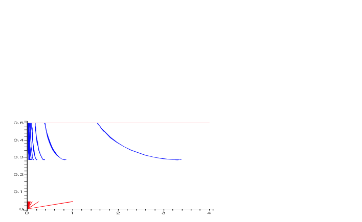
Figure 2: Phase diagram for near-extremal M5-branes on a circle.

In addition to the uniform and non-uniform phase, we also have the localized phase, corresponding to near-extremal M5-branes localized on a circle. This phase is considered in detail in Section 8.2. From (8.22) we see that $r\simeq 0.044\,\epsilon$ corresponds to the leading slope of the curve for the localized phase. This is also depicted in Figure 2.

We also have the copies of the localized and non-uniform phase, as explained above in Section 7.1 and 9.3. These are also depicted in Figure 2.

To draw all phases in the $(\epsilon,r)$ phase diagram for near-extremal M5-branes on a circle one would have to also consider solutions with Kaluza-Klein bubbles, i.e. with $r>1/2$. This we consider in a forthcoming publication [50].

10.2 Thermodynamics of non-uniform phase

Uniform phase

Before considering the thermodynamics of the non-uniform phase, we first review the thermodynamics of the uniform phase. The thermodynamics is

$$\hat{\mathfrak{t}}=1\ ,\ \ \hat{\mathfrak{f}}=0\ ,\ \ \hat{\mathfrak{s}}_{u}(\epsilon)=\epsilon\ .$$ (10.1)

Thus, the temperature is constant, the free energy is zero and the entropy grows linearly with energy. As we mention in Section 11 this is a signature of Hagedorn behavior of the thermodynamics with $\hat{\mathfrak{t}}=1$ being the Hagedorn temperature.

We see that the thermodynamics (10.1) of the uniform phase is of a rather singular nature. In the microcanonical ensemble we can put in an arbitrary amount of energy into the system without affecting the temperature. In the canonical ensemble we see that the temperature is fixed, so the heat capacity is infinite. One should therefore understand the thermodynamics (10.1) as being a special limit of the thermodynamics of near-extremal M5-branes on a circle. I.e. the hope is to find corrections to (10.1) or other phases of near-extremal M5-branes on a circle that describe the thermodynamics for temperatures $\hat{\mathfrak{t}}\neq 1$. For $\hat{\mathfrak{t}}\ll 1$ we have the localized phase, as considered in Section 8.2 (see also Section 11), but for $\hat{\mathfrak{t}}>1$ we need new input to determine the physics. This will be provided below.

Thermodynamics of non-uniform phase in microcanonical ensemble

We first consider the microcanonical ensemble, i.e. the thermodynamics for fixed energy. We use now the map (6.11) to find the temperature $\hat{\mathfrak{t}}$ and entropy $\hat{\mathfrak{s}}$ of the non-uniform phase of near-extremal M5-branes on a circle, using the data of Wiseman [11] for the temperature and entropy of the non-uniform black string branch. Using this we plot the non-uniform phase in the $(\epsilon,\hat{\mathfrak{s}})$ diagram as depicted in Figure 3. In this figure we also plotted the uniform phase using the thermodynamics (10.1), giving a straight line in the $(\epsilon,\hat{\mathfrak{s}})$ diagram.

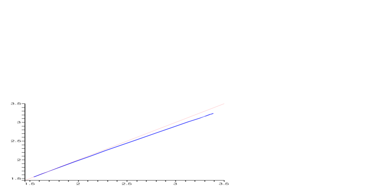
Figure 3: The entropy $\hat{\mathfrak{s}}(\epsilon)$ as a function of energy for near-extremal M5-branes on a circle.

As we clearly see in Figure 3 the non-uniform phase emanates from the uniform phase at the energy $\epsilon=\epsilon_{c}$, and has lower entropy than the uniform phase for a given energy $\epsilon$. Therefore, in the microcanonical ensemble the uniform phase is the dominant phase since it has higher entropy.

If we consider the behavior of the entropy near the energy $\epsilon=\epsilon_{c}$, we see from (9.14) that

$$\frac{\hat{\mathfrak{s}}(\epsilon)}{\hat{\mathfrak{s}}_{u}(\epsilon)}=1-0.05\cdot(\epsilon-\epsilon_{c})^{2}\ ,\ \ \epsilon_{c}=1.54\ .$$ (10.2)

for $0\leq\epsilon-\epsilon_{c}\ll 1$. This is in accordance with the numerical data plotted in Figure 3.

Thermodynamics of non-uniform phase in canonical ensemble

We now turn to the canonical ensemble, i.e. thermodynamics for fixed temperature. As stated above, we can use the map (6.11) to find the temperature $\hat{\mathfrak{t}}$ and entropy $\hat{\mathfrak{s}}$ for the non-uniform phase, from the data of Wiseman on non-uniform black strings [11]. Using in addition (6.10) to get the energy $\epsilon$, we can also find the free energy $\hat{\mathfrak{f}}=\epsilon-\hat{\mathfrak{t}}\hat{\mathfrak{s}}$. Therefore, we find the free energy as function of temperature $\hat{\mathfrak{f}}(\hat{\mathfrak{t}})$ for the non-uniform phase. This is plotted in Figure 4. Note that also the copies of the non-uniform phase are plotted in Figure 4, using that for the $k$’th copy $\hat{\mathfrak{f}}^{\prime}=k^{-2}\hat{\mathfrak{f}}$ and $\hat{\mathfrak{t}}^{\prime}=\hat{\mathfrak{t}}$.

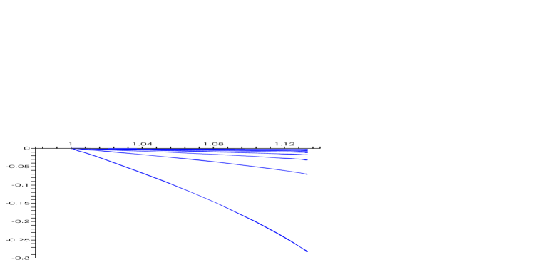
Figure 4: The free energy $\hat{\mathfrak{f}}(\hat{\mathfrak{t}})$ as a function of temperature for the non-uniform phase of near-extremal M5-branes on a circle, and for the copies of the non-uniform phase.

We see in Figure 4 that the free energy of the non-uniform phase is negative. This is also the case for the copies, although the free energy for these is higher. Therefore, the system prefers to be in the non-uniform phase rather than in one of its copy-phases, since the non-uniform phase has the lowest free energy.

We can also consider the heat capacity $c=\hat{\mathfrak{t}}\delta\hat{\mathfrak{s}}/\delta\hat{\mathfrak{t}}$ of the system. We have plotted this in Figure 5 for the non-uniform phase as a function of the temperature $\hat{\mathfrak{t}}$.

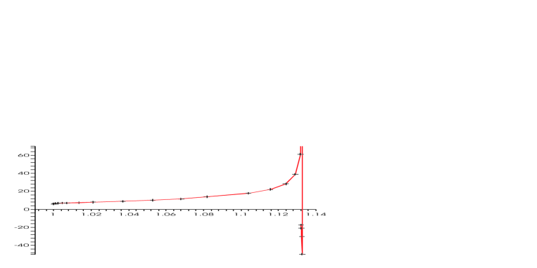
Figure 5: The heat capacity $c$ as function of the temperature $\hat{\mathfrak{t}}$ for the non-uniform phase of near-extremal M5-branes on a circle.

We see from Figure 5 that the heat capacity is positive, at least for $\hat{\mathfrak{t}}<1.13$. This means that the non-uniform phase is in fact a stable phase for near-extremal M5-branes on a circle, with temperatures $\hat{\mathfrak{t}}>1$. This is highly interesting since so far the only known stable phase for M5-branes on a circle has been the low temperature phase for $\hat{\mathfrak{t}}\ll 1$ where the M5-brane localizes on the circle. Here we see that there is a new stable phase with temperatures above the critical temperature $\hat{\mathfrak{t}}=1$.

In conclusion, it seems that the non-uniform phase for near-extremal M5-branes on a circle plays a crucial role for the thermal phase structure of near-extremal M5-branes on a circle in the canonical ensemble, since it provides a new phase with temperatures $\hat{\mathfrak{t}}>1$. This will be further commented on in Section 11, where we also relate it to the dual non-gravitational theory living on the NS5-brane.

Finally, we note that if we consider the free energy for $0\leq\hat{\mathfrak{t}}-1\ll 1$ we see from (9.16) that

$$\hat{\mathfrak{f}}(\hat{\mathfrak{t}})=-1.54\cdot(\hat{\mathfrak{t}}-1)-3.23\cdot(\hat{\mathfrak{t}}-1)^{2}$$ (10.3)

The numerical values in the expression can be found using Table 2.

11 New results for $(2,0)$ LST from M5-branes on a circle

In Section 8.2 and Section 10 we discussed the localized and non-uniform phases of near-extremal M5-branes on a circle. As we explain below, we have a duality between near-extremal M5-branes on a circle and $(2,0)$ Little String Theory. In the following we use this to give predictions for the thermal behavior of $(2,0)$ Little String Theory, using the results on near-extremal M5-branes on a circle.

M5-branes on a circle and $(2,0)$ LST

The $(2,0)$ Little String Theory (LST) is a $5+1$ dimensional non-gravitational string theory that is conjectured to live on the world-volume of the type IIA NS5-brane. The precise definition of $(2,0)$ LST (of type $A_{N-1}$) is that it is the $g_{s}\rightarrow 0$ limit of $N$ coincident NS5-branes with $l_{s}$ being fixed [33, 34, 35]. Here $g_{s}$ is the string coupling and $l_{s}$ is the string length.

$N$ coincident type IIA NS5-branes are S-dual to $N$ coincident M5-branes on a (transverse) circle, with the circumference of the circle $L$ related to the eleventh dimensional Planck length $l_{p}$ and the string coupling $g_{s}$ and string length $l_{s}$ as $l_{s}^{2}=2\pi l_{p}^{3}/L$ and $g_{s}^{2}=L^{3}/(2\pi l_{p})^{3}$. Therefore, we can alternatively define $(2,0)$ LST of type $A_{N-1}$ as being the $l_{p}\rightarrow 0$ limit of $N$ coincident M5-branes on a circle, with the circumference $L$ of the circle going to zero such that $L/l_{p}^{3}$ is fixed.

As conjectured in [31, 32], the near horizon limit of $N$ coincident M5-branes located at a point on a (transverse) circle is the supergravity dual of $(2,0)$ LST for large $N$. The low energy phase in the supergravity side corresponds to $AdS_{7}\times S^{4}$. This is dual to the 5+1 dimensional superconformal $(2,0)$ theory which is the low energy phase of $(2,0)$ LST. The high energy phase is the near-horizon limit of an M5-brane smeared on the circle, which is the S-dual supergravity solution to the type IIA NS5-brane. As explained in [14] the supergravity description of $(2,0)$ LST does not break down in the transition between the low- and high energy phases since the curvature of the eleven dimensional supergravity solution is always small.

If we turn on a temperature, the following duality is conjectured to be true [31, 32] (see also [14])

• Thermal $(2,0)$ LST of type $A_{N-1}$ is dual to $N$ coincident near-extremal M5-branes on a circle, for $N\gg 1$.

As for the zero-temperature duality, one expects the smeared M5-brane solution, which is S-dual to near-extremal type IIA NS5-branes, to be valid at high energies. The near-extremal NS5-brane has a constant temperature and the entropy is proportional to the energy (see (10.1)). This fits well with the conjecture that this solution is dual to a non-gravitational string theory [39, 31].

However, the fact that the temperature is constant (or, equivalently that the free energy is zero) for the near-extremal NS5-brane means that any correction to the thermodynamics, no matter how small, will contribute to the leading order behavior of the thermodynamics. Thus, to understand the thermodynamics of near-extremal NS5-branes, it seems crucial to study the corrections to the solution.

In [36, 37, 38] string corrections to the supergravity description were considered, with the result that the leading correction gives rise to a negative specific heat of the NS5-brane, and that the temperature of the near-extremal NS5-brane is larger than $\hat{T}_{\rm hg}$ [38].

In [14] it was advocated that one instead should look for a non-uniform phase of near-extremal M5-branes on a circle, in order to find a dual to the thermal $(2,0)$ LST. The expectation of [14] was that such a non-uniform phase would have positive specific heat, and could therefore provide a dual of thermal $(2,0)$ LST in a stable phase.

In the following we shall see that the new non-uniform phase of near-extremal M5-branes on a circle found in Section 10 provides a stable phase of $(2,0)$ LST in the canonical ensemble for a certain range of temperatures. This confirms in part the ideas of [14] since we find a new dual of thermal $(2,0)$ LST from a non-uniform phase.

Interpretation of non-uniform phase for $(2,0)$ LST

We now make the statement of the duality between $(2,0)$ LST of type $A_{N-1}$ and the near-extremal limit of $N$ coincident M5-branes on a circle more precise. We have defined the near-extremal limit by (5.2). By employing the IIA/M S-duality, one gets that the fixed quantities $g$ and $l$ in (5.2) are given as

$$g=\frac{(2\pi)^{5}l_{s}^{6}}{V_{5}}\ ,\ \ l=2\pi l_{s}\sqrt{N}\ .$$ (11.1)

where $l_{s}$ is the string length in type IIA string theory, that is kept fixed in the limit defining $(2,0)$ LST. One can now use (11.1) together with (5.10) and (5.11) as a dictionary between dimensionless and dimensionful quantities. Considering the thermodynamics of the uniform phase (10.1), we see that in dimensionful quantities we have

$$\hat{T}=\hat{T}_{\rm hg}\equiv\frac{1}{2\pi l_{s}\sqrt{N}}\ ,\ \ \hat{F}=0\ ,\ \ \hat{S}=\frac{1}{\hat{T}_{\rm hg}}E\ .$$ (11.2)

We see that this corresponds to the thermodynamics of a system near a Hagedorn temperature $\hat{T}_{\rm hg}$, since the entropy is proportional to the energy [39, 31].

We can now interpret the non-uniform phase of near-extremal M5-branes on a circle found in Section 10. If we consider the canonical ensemble, we found in Section 10 that the heat capacity is positive (see Figure 5), the free energy is negative (see Figure 4) and the temperature can vary in the range $[\hat{T}_{\rm hg},1.13\hat{T}_{\rm hg}]$ (using that $\hat{\mathfrak{t}}=\hat{T}/\hat{T}_{\rm hg}$). This means that this is a stable phase of near-extremal M5-branes on a circle, and by the duality conjecture this should describe thermal $(2,0)$ LST in that temperature range. We have thus found a stable phase of $(2,0)$ LST in the canonical ensemble for temperature above the Hagedorn temperature $\hat{T}_{\rm hg}$.

Notice that the copies of the non-uniform phase, as depicted in Figure 4 have positive heat capacity and they exist in the same temperature range, so they also correspond to stable phases of thermal $(2,0)$ LST. However, the free energy of these phases are higher than that of the non-uniform phase, so the non-uniform phase dominates over its copies.

Translating the dimensionless expression (10.3) for the free energy into dimensionful quantities, we see that the free energy for temperatures near the Hagedorn temperature, i.e. $0\leq\hat{T}-\hat{T}_{\rm hg}\ll\hat{T}_{\rm hg}$, is

$$\hat{F}(\hat{T})=-2\pi V_{5}N^{3}\hat{T}_{\rm hg}^{6}\left[1.54\cdot\left(\frac{\hat{T}}{\hat{T}_{\rm hg}}-1\right)+3.23\cdot\left(\frac{\hat{T}}{\hat{T}_{\rm hg}}-1\right)^{2}\right]\ .$$ (11.3)

It would interesting if one could reproduce this expression from the $(2,0)$ LST side.

Turning to the microcanonical ensemble, we see from Figure 3 that the uniform phase dominates over the non-uniform phase, since the uniform phase has higher entropy. Thus, for a fixed energy, the temperature is expected from this to decrease down to the Hagedorn temperature. It would be interesting to understand what the physics behind this is. Perhaps the resolution of this could be that the localized phase also exists in the same energy range as the non-uniform phase, but with higher entropy than the uniform phase.

Prediction for thermodynamics at low temperatures in $(2,0)$ LST

In addition to the new non-uniform phase that we interpreted above, we also have the new results for the localized phase found in Section 8.2.

The localized phase of near-extremal M5-branes on a circle corresponds to the low temperature/low energy phase of thermal $(2,0)$ LST. This is consistent with the fact that the localized phase dominates over the uniform phase, both in the canonical and microcanonical ensembles, for low temperature/low energy. Note that the infrared fixed point of $(2,0)$ LST is the superconformal $(2,0)$ theory, thus by considering the localized phase of near-extremal M5-branes for low temperatures (or energies) we find the corrections to the thermodynamics of the superconformal $(2,0)$ theory, as one moves away from the infrared fixed point.

The corrected free energy of the localized near-extremal M5-brane is computed from (8.25) with $d=5$ using the translation dictionary (11.1) to go to dimensionful quantities. In the canonical ensemble we then find the following expression for the corrected thermodynamics of the superconformal $(2,0)$ theory

$$\hat{F}(\hat{T})=-k_{\rm M5}V_{5}N^{3}\hat{T}^{6}\left[1+\frac{3\zeta(3)k_{\rm M5}}{2\pi^{3}}\left(\frac{\hat{T}}{\hat{T}_{\rm hg}}\right)^{6}+{\cal{O}}\left(\left(\frac{\hat{T}}{\hat{T}_{\rm hg}}\right)^{12}\right)\right]\ ,\ \ k_{\rm M5}=\frac{2^{6}\pi^{3}}{3^{7}}\ .$$ (11.4)

This shows that the dimensionless expansion parameter is $\delta=\hat{T}/\hat{T}_{\rm hg}$, as expected on physical grounds.

Note that one can obtain the free energy for the $k$’th copy of the localized phase from

$$\hat{F}_{(k)}(\hat{T})=k^{-2}\hat{F}(\hat{T})\ ,$$ (11.5)

for $k=1,2,...$. We see that the copy-phases have higher free energy than the localized phase, so the localized phase dominates over the copies.

We list here only the results for the canonical ensemble, both since this is the most interesting for comparison with calculations on the $(2,0)$ LST side, but also since one in any case easily can transform the result for the canonical ensemble to that of the microcanonical ensemble.

12 Predictions for supersymmetric Yang-Mills theories

In this section we apply the new results on near-extremal D-branes and the M2-brane on a transverse circle to obtain non-trivial predictions for the thermodynamics of the corresponding dual non-gravitational theories that live on these branes.

We first treat the case of near-extremal D0, D1, D2 and D3-branes on a circle. Then we discuss the case of the near-extremal M2-brane on a circle.

12.1 $(p+1)$-dimensional Yang-Mills theory on a circle

If we take the near-extremal limit of a D$p$-brane it is well known that the bulk dynamics decouples from the supersymmetric Yang-Mills (SYM) theory living on the brane. The near-extremal D$p$-brane is therefore conjectured to be a dual description of the strongly coupled large $N$ limit of ($p+1$)-dimensional SYM with 16 supercharges (on the manifold $\mathbb{R}^{p}$ for the spatial directions) [1, 5].

To determine what the dual field theories are for near-extremal D-branes on a circle we use T-duality. A near-extremal D$(p-1)$-brane on a transverse circle is T-dual to a D$p$-brane wrapped on a circle. It follows from this that the field theory dual of a near-extremal D$(p-1)$-brane on a transverse circle is that of a near-extremal D$p$-brane with a circle along the world-volume. We see from this that $N$ coincident near-extremal D$(p-1)$-branes on a transverse circle should be dual to $(p+1)$-dimensional SYM on $\mathbb{R}^{p-1}\times S^{1}$ with gauge group $SU(N)$ and 16 supercharges.

In particular, the phases of near-extremal D2-branes on a transverse circle are dual to those of ${\cal{N}}=4$ SYM theory in 3+1 dimensions on $\mathbb{R}^{2}\times S^{1}$ . Including the thermal time direction the field theory lives on $\mathbb{R}^{2}\times T^{2}$, where we define the torus here as $T^{2}\equiv S^{1}\times S^{1}_{T}$. Two other interesting examples are near-extremal D1 and D0-branes on a transverse circle which are respectively dual to 2+1 dimensional SYM on $\mathbb{R}\times S^{1}$ (i.e. including the thermal time direction on $\mathbb{R}\times T^{2}$) and 1+1 dimensional SYM theory on $S^{1}$ (i.e. including the thermal time direction on the torus $T^{2}$). In this section we restrict ourselves to the D0, D1, D2 and D3-branes on a circle.

We can thus use the results of Sections 8 and 9 to obtain predictions for the thermodynamics of the dual gauge theories described above. In particular, the localized phase should correspond to the low temperature/low energy regime, while the non-uniform phase corresponds to a new phase, emerging from the uniform phase, which describes the high temperature/high energy regime.

In order to make precise predictions for the SYM theory we should first understand better the dictionary between near-extremal D$(p-1)$-branes on a (transverse) circle and the SYM theory. To this end, define $L$ to be the circumference of the circle transverse to the D$(p-1)$-branes, $g_{s}$ to be the string coupling and $l_{s}$ the string length. In the T-dual theory, with the T-duality along the circle direction, we define instead $\hat{L}$ to be the circumference of the T-dual circle and $\hat{g}_{s}$ to be the T-dual string coupling. We have then that $L\hat{L}=(2\pi l_{s})^{2}$ and $g_{s}\hat{L}=2\pi l_{s}\hat{g}_{s}$. Using this along with the quantization condition for $N$ D$p$-branes in the T-dual theory, the near-extremal limit (5.2) and the definition of $l$ in (5.5), we get that $g$ and $l$ are given as

$${\rm D}(p-1)\;\,\mbox{on circle}\;\,:\qquad g=\frac{1}{(2\pi)^{3}N^{2}}\frac{\hat{L}^{p}}{V_{p-1}}\left(\lambda\hat{L}^{3-p}\right)^{2}\ ,\ \ l=\frac{\hat{L}}{\sqrt{2\pi}}\sqrt{\lambda\hat{L}^{3-p}}\ .$$ (12.1)

Here we wrote $g$ and $l$ in terms of the SYM theory variables, i.e. $N$ is the rank of the $SU(N)$ gauge group, $\lambda=g_{\rm YM}^{2}N$, $g_{\rm YM}^{2}=(2\pi)^{p-2}\hat{g}_{s}l_{s}^{p-3}$ and $\hat{L}$ is the circumference of the field theory circle $S^{1}$.

Note in particular that from $g$, $l$ and $\hat{T}$ we can form two independent dimensionless parameters, $l/g$ and $l\hat{T}$. These two parameters will play a physical role in the field theory expressions below.

We can now reinstate the dimensions in the thermodynamics, so that it can be written in terms of SYM variables. For this we recall the definition of $\epsilon$ in (5.10), of $\hat{\mathfrak{t}}$, $\hat{\mathfrak{s}}$ in (5.11) and of $\hat{\mathfrak{f}}$ in (7.12). It follows that given the thermodynamic functions $\hat{\mathfrak{s}}(\epsilon)$ and $\hat{\mathfrak{f}}(\hat{\mathfrak{t}})$ that we computed before, we can compute the entropy $\hat{S}$ and free energy $\hat{F}$ of the dual field theory with

$$\hat{S}(E)=\frac{l}{g}\hat{\mathfrak{s}}(gE)\ ,\ \ \hat{F}(\hat{T})=\frac{1}{g}\hat{\mathfrak{f}}(l\hat{T})\ ,$$ (12.2)

where $E$ and $\hat{T}$ are the energy and temperature in the field theory.

We now present the new results for ($p+1$)-dimensional SYM theory on $\mathbb{R}^{p-1}\times S^{1}$ that follow from the localized and non-uniform phases of near-extremal D$(p-1)$-branes. We remind the reader that these phases are directly linked via U-duality and the near-extremal limit to the localized black hole phase and non-uniform black string phase of pure gravity on $\mathcal{M}^{10-p}\times S^{1}$. In the quantitative analysis below we focus on the canonical ensemble.

Uniform phase: High temperature phase of SYM on a circle

We begin by considering the uniform phase of near-extremal D$(p-1)$-branes on a circle. This corresponds to the high temperature phase of ($p+1$)-dimensional SYM theory on $\mathbb{R}^{p-1}\times S^{1}$. This is easily understood on physical grounds since high temperatures correspond to short distances, and this means that one does not see the compact direction in $\mathbb{R}^{p-1}\times S^{1}$, i.e. the circumference $\hat{L}$ should only appear as a trivial proportionality factor in the free energy. This is precisely what we get for the uniform phase since it corresponds to a uniformly smeared near-extremal D$(p-1)$-brane, which has the same thermodynamics as a near-extremal D$p$-brane. It is not difficult to check this explicitly using the thermodynamics (7.6) and the translation dictionary (12.2). The result for the free energy in the uniform phase is then

$$\hat{F}^{\rm u}_{{\rm SYM}(p+1)}(\hat{T})=\hat{F}^{\rm u}_{{\rm D}(p-1)}(\hat{T})=-k_{p}V_{p-1}\hat{L}N^{2}\lambda^{-\frac{3-p}{5-p}}\hat{T}^{2\frac{7-p}{5-p}}\ ,$$ (12.3)

where the coefficients $k_{p}$ are given in Table 3. The expression (12.3) is indeed the familiar result for the free energy of the D$p$-brane theory, with $V_{p}=V_{p-1}\hat{L}$.

Localized phase: Low temperature phase of SYM on a circle

We now turn to the localized phase, corresponding to the low temperature phase of ($p+1$)-dimensional SYM theory on $\mathbb{R}^{p-1}\times S^{1}$. Low temperatures correspond to large distances in the SYM theory, so in this regime the presence of the circle enters in a non-trivial manner. If one consider free ($p+1$)-dimensional SYM theory on $\mathbb{R}^{p-1}\times S^{1}$, it is clear that one has a tower of Kaluza-Klein states for the circle, and that the lowest Kaluza-Klein mode corresponds to free $p$-dimensional SYM theory on $\mathbb{R}^{p-1}$. Similarly, we shall see below that for the temperature $\hat{T}$ going to zero, the leading order thermodynamics for the localized phase of D$(p-1)$-branes on a circle corresponds to the thermodynamics of a near-extremal D$(p-1)$-brane, which is dual to strongly coupled $p$-dimensional SYM theory on $\mathbb{R}^{p-1}$. The corrections to the leading order thermodynamics for the localized phase found in Section 8 then correspond to including corrections from the Kaluza-Klein modes on the circle.

Using the expressions for the corrected free energy in (8.25) along with the translation dictionary (12.2), (12.1) we find for the localized phase of thermal ($p+1$)-dimensional SYM theory on $\mathbb{R}^{p-1}\times S^{1}$ the free energy

$$\hat{F}^{\rm loc}_{{\rm SYM}(p+1)}(\hat{T})=\hat{F}^{\rm loc}_{{\rm D}(p-1)}(\hat{T})$$ (12.4)

$$\simeq-k_{p-1}V_{p-1}N^{2}\left(\frac{\lambda}{\hat{L}}\right)^{-\frac{4-p}{6-p}}\hat{T}^{2\frac{8-p}{6-p}}\left\{1+\frac{2(9-p)\zeta(8-p)k_{p-1}}{(6-p)^{2}(2\pi)^{3}\Omega_{9-p}}\left[\hat{L}\hat{T}\sqrt{\lambda\hat{L}^{3-p}}\right]^{2\frac{8-p}{6-p}}\right\}\ .$$

Here the coefficients $k_{p}$ are listed in Table 3.

$p$	0	1	2	3	4
$k_{p}$	$(2^{21}3^{2}5^{7}7^{-19}\pi^{14})^{1/5}$	$2^{4}3^{-4}\pi^{5/2}$	$(2^{13}3^{5}5^{-13}\pi^{8})^{1/3}$	$2^{-3}\pi^{2}$	$2^{5}3^{-7}\pi^{2}$

Table 3: Coefficients for the free energy of D$p$-branes.

Note first of all that the leading term in (12.4) is in perfect agreement with the expected result for the strong coupling limit of the $p$-dimensional SYM theory. In particular, we observe the correct ’t Hooft coupling $\lambda/\hat{L}$ that follows from compactifying the $(p+1)$-dimensional theory. Moreover, (12.4) gives a quantitative prediction for the first correction term in terms of the dimensionless parameter

$$\delta=\hat{L}\hat{T}\sqrt{\lambda\hat{L}^{3-p}}\ .$$ (12.5)

The next corrections will be of order $(\delta^{2\frac{8-p}{6-p}})^{2}$. It would be highly interesting if one could find a way to reproduce the corrections computed above from the field theory side.

The explicit expressions of (12.4) for the cases $p=1,2,3$ and 4 are

$$\hat{F}^{\rm loc}_{{\rm SYM}(1+1)}(\hat{T})=\hat{F}^{\rm loc}_{{\rm D}0}(\hat{T})$$ (12.6)

$$=-k_{0}N^{2}\left(\frac{\lambda}{\hat{L}}\right)^{-3/5}\hat{T}^{14/5}\left\{1+\frac{21\zeta(7)k_{0}}{80\pi^{7}}(\lambda^{1/2}\hat{L}^{2}\hat{T})^{14/5}+{\cal{O}}\left((\lambda^{1/2}\hat{L}^{2}\hat{T})^{28/5}\right)\right\}\ ,$$

$$\hat{F}^{\rm loc}_{{\rm SYM}(2+1)}(\hat{T})=\hat{F}^{\rm loc}_{{\rm D}1}(\hat{T})$$ (12.7)

$$=-k_{1}V_{1}N^{2}\left(\frac{\lambda}{\hat{L}}\right)^{-1/2}\hat{T}^{3}\left\{1+\frac{k_{1}}{2880\pi}\left(\lambda^{1/2}\hat{L}^{3/2}\hat{T}\right)^{3}+{\cal{O}}\left((\lambda^{1/2}\hat{L}^{3/2}\hat{T})^{6}\right)\right\}\ ,$$

$$\hat{F}^{\rm loc}_{{\rm SYM}(3+1)}(\hat{T})=\hat{F}^{\rm loc}_{{\rm D}2}(\hat{T})$$ (12.8)

$$=-k_{2}V_{2}N^{2}\left(\frac{\lambda}{\hat{L}}\right)^{-1/3}\hat{T}^{10/3}\left\{1+\frac{5\zeta(5)k_{2}}{32\pi^{6}}\left(\lambda^{1/2}\hat{L}\hat{T}\right)^{10/3}+{\cal{O}}\left((\lambda^{1/2}\hat{L}\hat{T})^{20/3}\right)\right\}\ ,$$

$$\hat{F}^{\rm loc}_{{\rm SYM}(4+1)}(\hat{T})=\hat{F}^{\rm loc}_{{\rm D}3}(\hat{T})$$ (12.9)

$$=-k_{3}V_{3}N^{2}\hat{T}^{4}\left\{1+\frac{k_{3}}{288\pi^{2}}\left(\lambda^{1/2}\hat{L}^{1/2}\hat{T}\right)^{4}+{\cal{O}}\left((\lambda^{1/2}\hat{L}^{1/2}\hat{T})^{8}\right)\right\}\ ,$$

where we recall that in each case $\lambda$ is the ’t Hooft coupling of the ($p+1$)-dimensional SYM theory.

We note that the corresponding results in the microcanonical ensemble are easily obtained using the corrected entropy (8.24) of the localized near-extremal branes and (12.1), (12.2).

Non-uniform phase: New phase in SYM on a circle

Turning to the non-uniform phase of near-extremal $D(p-1)$-branes on a circle, we have that the results of Section 9 for the non-uniform phase give us i) a prediction of the existence of a new phase of ($p+1$)-dimensional SYM theory on $\mathbb{R}^{p-1}\times S^{1}$ at intermediate temperatures, and ii) the first correction to the thermodynamics around the point where this phase connects to the uniform phase.

In particular, using the expressions for the corrected free energy in (9.16) along with the translation dictionary (12.2), (12.1) we find for the non-uniform phase of thermal ($p+1$)-dimensional SYM theory on $\mathbb{R}^{p-1}\times S^{1}$ the free energy

$$F^{\rm nu}_{{\rm SYM}(p+1)}(\hat{T})=F^{\rm nu}_{{\rm D}(p-1)}(\hat{T})$$ (12.10)

$$\simeq-(2\pi)^{3}V_{p-1}N^{2}\lambda\hat{L}^{3-2p}\left[\frac{5-p}{9-p}\epsilon_{c}+\hat{\mathfrak{t}}_{c}\hat{\mathfrak{s}}_{c}\left(\frac{\hat{T}}{\hat{T}_{c}}-1\right)+\frac{\hat{\mathfrak{t}}_{c}c}{2}\left(\frac{\hat{T}}{\hat{T}_{c}}-1\right)^{2}\right]\ .$$

Here the critical temperature is given by

$$\hat{T}_{c}=\frac{\hat{\mathfrak{t}}_{c}}{\hat{L}}\sqrt{\frac{2\pi}{\lambda\hat{L}^{3-p}}}\ .$$ (12.11)

and the values for $\hat{\mathfrak{t}}_{c}$, $\epsilon_{c}$, $\hat{\mathfrak{s}}_{c}$ and $c$ can be read off from Table 2 using $d=10-p$. Note that the first term in the expression (12.10) corresponds to $\hat{F}^{\rm u}_{{\rm SYM}(p+1)}(\hat{T}_{c})$, i.e. the free energy (12.3) of the uniform phase evaluated at the critical temperature, while the second term is $-\hat{S}^{\rm u}_{{\rm SYM}(p+1)}(\hat{T}_{c})(\hat{T}-\hat{T}_{c})$, and hence involves the entropy of the uniform phase evaluated at the critical temperature. The third term contains the departure of the free energy of the uniform phase in this non-uniform phase.

As for the localized phase, the corresponding results for the non-uniform phase in the microcanonical ensemble are not difficult to obtain using the corrected entropy (9.14) of the localized near-extremal branes and (12.2), (12.1).

It would be very interesting to understand the new results (12.4) and (12.10) for thermal $(p+1)$-dimensional SYM theory on $\mathbb{R}^{p-1}\times S^{1}$ from the gauge theory side.

Copies of the localized and non-uniform phase

Since both the localized and non-uniform phase of near-extremal branes have copies, we also have copies of the thermal $(p+1)$-dimensional SYM phases obtained above. Using (7.7) the free energy of the $k$’th copy is given by

$$(\hat{F}_{{\rm SYM}(p+1)})_{(k)}(\hat{T})=k^{p-7}\hat{F}_{{\rm SYM}(p+1)}(k^{(5-p)/2}\hat{T})\ ,\ \ k=1,2,3,...\ ,$$ (12.12)

in terms of either $\hat{F}_{{\rm SYM}(p+1)}^{\rm loc}$ given in (12.4) or $\hat{F}_{{\rm SYM}(p+1)}^{\rm nu}$ given in (12.10)

12.2 New results in (2+1)-dimensional Yang-Mills theory

In this section we consider near-extremal M2-branes on a circle. By IIA/M S-duality, this is dual to a near-extremal D2-brane. Therefore, it is conjectured that $N$ coincident near-extremal M2-branes on a circle are dual to (2+1)-dimensional SYM theory with 16 supercharges with gauge group $SU(N)$ (on the non-compact space $\mathbb{R}^{2}$), $N\gg 1$ [1, 5]. We see that this is analogous to the near-extremal M5-brane on a circle and the duality to $(2,0)$ LST in Section 11.

In more detail, we take the circle transverse to the M2-brane to have circumference $L=2\pi g_{s}l_{s}$, and using the quantization condition on the M2-branes together with (5.2) and (5.5) we get

$$g=\frac{(2\pi)^{2}}{V_{2}}\frac{N^{3}}{\lambda^{3}}\ ,\ \ l=2\pi\frac{N^{3/2}}{\lambda}\ ,$$ (12.13)

where $\lambda=g_{\mathrm{YM}}^{2}N=g_{s}l_{s}^{-1}N$. This provides the dictionary for translating the results of the near-extremal M2-branes on a circle to the SYM theory.

As we shall see, the localized and non-uniform phase of the near-extremal M2-brane on a circle provide us with new information for thermal (2+1)-dimensional SYM theory on $\mathbb{R}^{2}$. Note that the results below are written in the canonical ensemble.

Uniform phase: High temperature phase

The uniform phase of near-extremal M2-branes on a circle corresponds to the high temperature/high energy limit of thermal (2+1)-dimensional SYM, i.e. the field theory dual of near-extremal D2-branes. We can check this explicitly using the thermodynamics (7.6) together with (12.2) and (12.13). The result for the free energy in the uniform phase is

$$\hat{F}^{\rm UV}_{\rm SYM(2+1)}(\hat{T})=\hat{F}^{\rm u}_{{\rm M}2}(\hat{T})=-k_{2}V_{2}N^{2}\lambda^{-1/3}\hat{T}^{10/3}\ ,$$ (12.14)

where the coefficient $k_{2}$ is given in Table 3. This is indeed the familiar result for the free energy of the near-extremal D2-brane theory.

Localized phase: Low temperature phase

The localized phase of near-extremal M2-branes on a circle corresponds to the low temperature/low energy limit of thermal (2+1)-dimensional SYM. The infrared fixed point of (2+1)-dimensional SYM is a superconformal field theory with $SO(8)$ R-symmetry, which for large $N$ is dual to the near-extremal M2-brane solution. The corrections obtained for the localized phase thus compute the corrections to the M2-brane theory as we move away from the infrared fixed point.

In particular, using $d=8$ in (8.25) together with (12.2) and (12.13) we then obtain the corrected free energy of the localized M2-brane phase as

$$\hat{F}_{{\rm SYM}(2+1)}^{\rm IR}(\hat{T})=\hat{F}_{\rm M2}^{\rm loc}(\hat{T})$$ (12.15)

$$=-k_{\rm M2}V_{2}N^{3/2}\hat{T}^{3}\left[1+\frac{\pi^{4}k_{\rm M2}}{90}\left(\frac{N^{3/2}\hat{T}}{\lambda}\right)^{3}+{\cal{O}}\left(\left(\frac{N^{3/2}\hat{T}}{\lambda}\right)^{6}\right)\right]\ ,\ \ k_{\rm M2}=\frac{2^{7/2}\pi^{2}}{3^{4}}\ .$$

Note that the dimensionless expansion parameter is $\delta=N^{3/2}\hat{T}/\lambda$ where $\lambda$ is the ’t Hooft coupling of the (2+1)-dimensional SYM theory.

Non-uniform phase: New phase in 2+1 dimensional SYM

For the non-uniform phase of the near-extremal M2-brane on a circle, the results of Section 9 give us i) a prediction of the existence of a new non-uniform phase of uncompactified ($2+1$)-dimensional SYM theory on $\mathbb{R}^{2}$ at intermediate temperatures and ii) the first correction to the thermodynamics around the point where this phase connects to the uniform phase.

In particular, using the expressions for the corrected free energy in (9.16) along with the translation dictionary (12.2), (12.13) we find for the non-uniform phase of thermal ($2+1$)-dimensional SYM theory on $\mathbb{R}^{2}$ the free energy

$$\hat{F}^{\rm UV^{\prime}}_{{\rm SYM}(2+1)}(\hat{T})=\hat{F}^{\rm nu}_{{\rm M}2}(\hat{T})\simeq-\frac{V_{2}}{(2\pi)^{2}}\frac{\lambda^{3}}{N^{3}}\left[\frac{3}{7}\epsilon_{c}+\hat{\mathfrak{t}}_{c}\hat{\mathfrak{s}}_{c}\left(\frac{\hat{T}}{\hat{T}_{c}}-1\right)+\frac{\hat{\mathfrak{t}}_{c}c}{2}\left(\frac{\hat{T}}{\hat{T}_{c}}-1\right)^{2}\right]$$ (12.16)

Here the critical temperature is given by

$$\hat{T}_{c}=\frac{\lambda}{2\pi N^{3/2}}\hat{\mathfrak{t}}_{c}\ ,\ \ \hat{\mathfrak{t}}_{c}=0.97\ ,$$ (12.17)

and one should substitute $\epsilon_{c}=0.46$, $\hat{\mathfrak{s}}_{c}=0.68$ and $c=1.14$ which are read off for $d=8$ from Table 2.

As for the case of SYM on a circle, it would be interesting to understand the new results (12.15) and (12.16) for uncompactified (2+1)-dimensional SYM theory from the gauge theory side.

Copies of the localized and non-uniform phase

Since both the localized and non-uniform phase of near-extremal branes have copies, we also have copies of the thermal uncompactified ($2+1$)-dimensional SYM phases obtained above. Using (7.7) the free energy of the $k$’th copy is given by

$$(\hat{F}_{{\rm SYM}(2+1)})_{(k)}(\hat{T})=\frac{1}{k^{5}}\hat{F}_{{\rm SYM}(p+1)}(k^{3/2}\hat{T})\ ,\ \ k=1,2,3,...\ ,$$ (12.18)

in terms of either $\hat{F}_{{\rm SYM}(p+1)}^{\rm IR}$ given in (12.15) or $\hat{F}_{{\rm SYM}(p+1)}^{\rm UV^{\prime}}$ given in (12.16)

13 Discussion and conclusions

We conclude the paper with the following remarks and open problems:

Comparison to weakly coupled SYM theory on a circle: In Section 12.1 we saw that we can give quantitative predictions for the thermodynamics of $(p+1)$-dimensional SYM theory on $\mathbb{R}^{p-1}\times S^{1}$, using the results on Kaluza-Klein black holes. One of the central ingredients is that the free energy is expressible as a function of the variable $\hat{\mathfrak{t}}\sim\sqrt{\lambda\hat{L}^{3-p}}\hat{L}\hat{T}$. Here $\lambda\hat{L}^{3-p}$ should be large in order for the supergravity description to hold, which means the SYM theory is in the strongly coupled regime. Thus, the scale in which we shift between the low temperature and high temperature regimes is around $\hat{\mathfrak{t}}\sim 1$, i.e. when $\hat{L}\hat{T}\sim 1/\sqrt{\lambda\hat{L}^{3-p}}$. We thus see that this scale is lower than for the free field theory, where it is instead at $\hat{L}\hat{T}\sim 1$. Also, for the localized phase we see that the expansion of the free energy for low temperatures is in powers of $\hat{\mathfrak{t}}$. Therefore, it is not clear if the predictions of Section 12.1 can be connected to thermodynamics of weakly coupled field theory in a quantitative manner. Perhaps a double-scaling limit could be engineered to make such a quantitative connection. However, it would in any case be interesting to examine free $(p+1)$-dimensional SYM on $\mathbb{R}^{p-1}\times S^{1}$ to see if there should be at least a qualitative similarity of the thermodynamics. In particular, it would be interesting if one could find a similar new non-uniform phase as the one we predicted should be there in the strongly coupled regime.

$(2,0)$ LST and near-extremal M5-branes on a circle: We have seen in Sections 10 and 11 that the non-uniform phase of near-extremal M5-branes on a circle predicts a new stable phase for the dual $(2,0)$ LST in the canonical ensemble, with temperatures above the Hagedorn temperature. This would be interesting to understand from the Little String Theory side.

Gregory-Laflamme type instability and Gubser-Mitra conjecture: We have shown that one non-trivial consequence of the map from Kaluza-Klein black holes to non- and near-extremal branes is that there exists a non-uniform phase for both these classes of branes, emanating from the uniform phase. In particular, the Gregory-Laflamme mass $\mu_{\rm GL}$ of the uniform black string branch is mapped onto a critical mass $\bar{\mu}_{c}$ of the uniform non-extremal branch and a critical energy $\epsilon_{c}$ of the uniform near-extremal branch. This, together with the fact that the entropy of the localized phase is higher than that of the uniform phase for small energies (above extremality), strongly suggests that non-/near-extremal branes on a circle have a critical mass/energy below which the uniform phase is classically unstable. It seems possible that one could use the boost and U-duality transformation of Section 4.1 to show that the unstable mode for the neutral uniform black string transforms into an unstable mode of the non-/near-extremal brane on a circle. It would be interesting to further examine this.

A related issue is the possibility of a counter-example to the Gubser-Mitra conjecture [27, 28, 29], stating that a black brane with a non-compact translational symmetry is free of dynamical instabilities if and only if it is locally thermodynamically stable. The uniform near-extremal branch has a translational symmetry and (for $d>5$) a positive heat capacity, so if indeed near-extremal branes are classically unstable for energies below $\epsilon_{c}$, this would be in contradiction to the conjecture.

On conjectures of Horowitz and Maeda: Another interesting consequence of the results of this paper is obtained if we revisit the results and conjectures of Horowitz and Maeda in [13, 26]. In [13] it was conjectured that there exists a non-uniform black string branch for arbitrarily small masses, with entropy higher than that of the uniform black string branch. This conjecture was based on the result that it would take infinite “time” (i.e. affine parameter on the horizon) to change the topology of the horizon in a classical evolution. Furthermore, in [26] it was conjectured that for the D3, M2 and M5-branes on a (transverse) circle, new non-uniform phases exist with arbitrarily small energy and with entropy higher than that of the uniform phase. The conjecture was based on a construction of suitable initial data and on the conjecture of [13].

But if we assume that the conjecture of [13] is correct, we see that using the map from static and neutral Kaluza-Klein black holes to near-extremal branes on a circle, we get immediately that the conjectured small mass non-uniform black string branch implies the existence of a low-energy non-uniform phase of near-extremal branes on a circle, with entropy higher than that of the uniform phase. This includes in particular the D3, M2 and M5-branes, but in addition also the other $1/2$ BPS branes of string theory and M-theory.

However, it is important to emphasize that it is unclear whether the conjecture of [13] is correct. The above point is therefore, so far, more of a theoretical nature.

Non- and near-extremal bubble-black hole sequences: Recently, it was found [22] that in the region $1/(d-2)<n\leq d-2$ of the $(\mu,n)$ phase diagram of Kaluza-Klein black holes involve solutions that combine event horizons and static Kaluza-Klein bubbles. We leave the application of the map to these bubble-black hole sequences to a future publication [50].

New phases: More generally, we emphasize that any new phase that one may find in the $(\mu,n)$ phase diagram, analytically or numerically, will immediately generate via the map new non- and near-extremal phases. Moreover, any such new phase would immediately have consequences for the non-gravitational theories dual to the near-extremal phases. Finally, it should be clear that any non-trivial phase structure and phase transition for Kaluza-Klein black holes, such as the conjectured topology-changing black string/hole transition, will have an interesting counterpart in the dual non-gravitational theories.

Appendix A Energy and tension for near-extremal branes

In this appendix we use the general expressions (5.7), (5.8) to compute the energy and tension for the class of near-extremal branes on a circle that fall into the ansatz (6.14)-(6.16). As remarked at the end of Section 6.3, this is an important check on the consistency of the near-extremal limit. Moreover, since these branes are not asymptotically flat, it also provides a useful illustration of the general formula for tension in non-asymptotically flat spaces given in Ref. [25]. Following the discussion of Section 5, the reference space that we use for the near-extremal $p$-brane is the near-horizon limit of the extremal $p$-brane on a circle, the asymptotics of which is given in (5.3)-(5.5).

To compute the energy and tension, we first recall a useful expression for the extrinsic curvature $\mathcal{K}^{(D-2)}$ entering the computation of these quantities. We have

$$\mathcal{K}^{(D-2)}=\frac{1}{\sqrt{g_{RR}}}\partial_{R}\log\sqrt{h}\ .$$ (A.1)

Here $h=\sqrt{\det h^{D-2}}$ with $h^{D-2}$ the metric obtained from $g$ by omitting $t,R$ when computing $E$ and omitting $v,r$ when computing $\hat{\mathcal{T}}$. For clarity we denote the corresponding expressions by $\mathcal{K}_{t}$ and $\mathcal{K}_{v}$ respectively.

For the computation below we use that in the metric (6.14)-(6.16) we have asymptotically

$$g_{tt}\simeq\hat{H}^{-\frac{d-2}{D-2}}\left(-1+\frac{\hat{c}_{t}}{R^{d-3}}\right)\ ,\ \ g_{uu}\simeq\hat{H}^{-\frac{d-2}{D-2}}\ ,$$ (A.2)

$$g_{RR}\simeq\hat{H}^{\frac{p+1}{D-2}}\left(1+\frac{\hat{c}_{R}}{R^{d-3}}\right)\ ,\ \ g_{vv}\simeq\hat{H}^{\frac{p+1}{D-2}}\left(1+\frac{\hat{c}_{v}}{R^{d-3}}\right)\ ,\ \ g_{\Omega\Omega}\simeq\hat{H}^{\frac{p+1}{D-2}}R^{2}\left(1+\frac{\hat{c}_{\Omega}}{R^{d-3}}\right)\ ,$$ (A.3)

with

$$\hat{c}_{t}=R_{0}^{d-3}\ ,\ \ \hat{c}_{R}=(1-\chi)R_{0}^{d-3}\ ,\ \ \hat{c}_{v}=(d-3)\chi R_{0}^{d-3}\ ,\ \ \hat{c}_{\Omega}=-\chi R_{0}^{d-3}\ ,$$ (A.4)

where we used (2.12). It is then not difficult to use (A.1) and compute

$$\mathcal{K}_{t}\simeq\left[\hat{H}^{\frac{p+1}{D-2}}(R_{\rm m})\left(1+\frac{\hat{c}_{R}}{R_{\rm m}^{d-3}}\right)\right]^{-1/2}\frac{1}{R_{\rm m}}\left[\frac{d-1}{2}-\frac{d-3}{2R_{\rm m}^{d-3}}(\hat{c}_{v}+\hat{c}_{\Omega})\right]\ ,$$ (A.5)

$$\mathcal{K}_{v}=\left[\hat{H}^{\frac{p+1}{D-2}}(R_{\rm m})\left(1+\frac{\hat{c}_{R}}{R_{\rm m}^{d-3}}\right)\right]^{-1/2}\frac{1}{R_{\rm m}}\left[d-2-\frac{d-3}{2R_{\rm m}^{d-3}}(-\hat{c}_{t}+\hat{c}_{\Omega})\right]\ ,$$ (A.6)

where $R_{m}$ is sent to infinity. Next we compute the extrinsic curvature of the reference space in both cases, giving

$$\mathcal{K}_{t}^{(0)}=\left[\hat{H}^{\frac{p+1}{D-2}}(R_{\rm eff})\right]^{-1/2}\frac{d-1}{2\,R_{\rm eff}}\ ,\ \ \mathcal{K}_{v}^{(0)}=\left[\hat{H}^{\frac{p+1}{D-2}}(R_{\rm eff})\right]^{-1/2}\frac{d-2}{R_{\rm eff}}\ ,$$ (A.7)

where we used that asymptotically $\hat{r}\simeq R$ and $\hat{z}\simeq v$ [14]. The relation between $R_{\rm m}$ and $R_{\rm eff}$ is obtained by imposing that the radius of the $S^{d-2}$ in the brane space time is equal to that of the radius of the $S^{d-2}$ in the reference space. This gives

$$\left[\hat{H}^{\frac{p+1}{D-2}}(R_{\rm eff})\right]^{1/2}R_{\rm eff}=\left[\hat{H}^{\frac{p+1}{D-2}}(R_{\rm m})\left(1+\frac{\hat{c}_{\Omega}}{R_{\rm m}^{d-3}}\right)\right]^{1/2}R_{\rm m}\ ,$$ (A.8)

and a little algebra then shows

$$\mathcal{K}_{t}-\mathcal{K}_{t}^{(0)}\simeq\frac{1}{2\,R_{\rm m}^{d-2}}\left[\hat{H}^{\frac{p+1}{D-2}}(R_{\rm m})\right]^{-1/2}\left[\frac{d-1}{2}(\hat{c}_{\Omega}-\hat{c}_{R})-(d-3)(\hat{c}_{v}+(d-2)\hat{c}_{\Omega})\right]\ ,$$ (A.9)

$$\mathcal{K}_{v}-\mathcal{K}_{v}^{(0)}\simeq\frac{1}{2\,R_{\rm m}^{d-2}}\left[\hat{H}^{\frac{p+1}{D-2}}(R_{\rm m})\right]^{-1/2}\left[(d-2)(\hat{c}_{\Omega}-\hat{c}_{R})-(d-3)(-\hat{c}_{t}+(d-2)\hat{c}_{\Omega})\right]\ .$$ (A.10)

Finally, we need for each case the lapse functions and integration measures: $N_{t}=(g_{tt}^{(0)})^{1/2}=\hat{H}^{-\frac{d-2}{2(D-2)}}$, $\sqrt{g_{D-2}}=\sqrt{\hat{H}}R^{d-2}$ for the energy and $N_{v}=(g_{vv}^{(0)})^{1/2}=\hat{H}^{\frac{p+1}{2(D-2)}}$, $\sqrt{g_{D-2}}=R^{d-2}$ for the tension. Using all this in (5.7), (5.8) we have the final results

$$E=\frac{\Omega_{d-2}}{(2\pi)^{d-3}g}\left[\frac{d-1}{2}(\hat{c}_{R}-\hat{c}_{\Omega})+(d-3)(\hat{c}_{v}+(d-2)\hat{c}_{\Omega})\right]\ ,$$ (A.11)

$$\hat{\mathcal{T}}=\frac{\Omega_{d-2}}{(2\pi)^{d-2}g}\left[(d-2)(\hat{c}_{R}-\hat{c}_{\Omega})+(d-3)(-\hat{c}_{t}+(d-2)\hat{c}_{\Omega})\right]\ ,$$ (A.12)

for the energy and tension for near-extremal $p$-branes on a circle. Substituting the values (A.4) and using the definitions (5.10) we then find the results given in (6.17) for $\epsilon$ and $r$.

We also quote the result for the tension in the world volume of the brane

$$L_{i}^{(u)}\hat{\mathcal{T}}_{i}^{(u)}=\frac{\Omega_{d-2}}{(2\pi)^{d-3}g}\left[\frac{d-1}{2}(\hat{c}_{R}-\hat{c}_{\Omega})+(d-3)(-\hat{c}_{t}+\hat{c}_{v}+(d-2)\hat{c}_{\Omega})\right]\ ,$$ (A.13)

which easily follows from a similar computation as the one given above. Substituting the values (A.4) and using the definitions (5.10) this gives the expression for $r_{u}$ given in (6.19).

Appendix B Flat space in $(\tilde{\rho},\tilde{\theta})$ coordinates

In this appendix we review the flat space metric of $\mathcal{M}^{d}\times S^{1}$ in the $(\tilde{\rho},\tilde{\theta})$ coordinates which was used in [18] to write down the metric of small black holes on the cylinder.

To write down the metric we need the function [14]

$$F(r,z)=\sum_{k=-\infty}^{\infty}\frac{1}{(r^{2}+(z-2\pi k)^{2})^{\frac{d-2}{2}}}\ ,$$ (B.1)

that enters the Newtonian potential for a black hole on the cylinder. This definition employs cylindrical coordinates $(r,z)$, which are related to spherical coordinates $(\rho,\theta)$ via

$$r=\rho\sin\theta\ ,\ \ z=\rho\cos\theta\ .$$ (B.2)

In terms of the latter coordinates the function in (B.1) is denoted by $F(\rho,\theta)$, which for $\rho\ll 1$ can be expanded as

$$F(\rho,\theta)=\frac{1}{\rho^{d-2}}+\frac{2\zeta(d-2)}{(2\pi)^{d-2}}+\frac{\zeta(d)}{(2\pi)^{d}}(d-2)\left[d\cos^{2}\theta-1\right]\rho^{2}+\mathcal{O}(\rho^{4})\ .$$ (B.3)

The function $F(\rho,\theta)$ enters the coordinate transformation to the final $(\tilde{\rho},\tilde{\theta})$ coordinates, which are given by

$$\tilde{\rho}^{d-2}=\frac{1}{F(\rho,\theta)}\ ,$$ (B.4)

$$(\sin\tilde{\theta})^{d-2}\partial_{\rho}\tilde{\theta}=\frac{\rho^{d-3}}{d-2}(\sin\theta)^{d-2}\partial_{\theta}F\ ,\ \ (\sin\tilde{\theta})^{d-2}\partial_{\theta}\tilde{\theta}=-\frac{\rho^{d-1}}{d-2}(\sin\theta)^{d-2}\partial_{\rho}F\ .$$ (B.5)

Using the expansion (B.3) this can be expanded for $\rho\ll 1$ as

$$\rho=\tilde{\rho}\left(1+\frac{2\zeta(d-2)}{(d-2)(2\pi)^{d-2}}\tilde{\rho}^{d-2}+\mathcal{O}(\tilde{\rho}^{d})\right)\ ,$$ (B.6)

$$\sin^{2}\theta=\sin^{2}\tilde{\theta}\left(1+\frac{4\zeta(d)}{(2\pi)^{d}}\cos^{2}\tilde{\theta}\tilde{\rho}^{d}+\mathcal{O}(\tilde{\rho}^{d+2})\right)\ .$$ (B.7)

Finally, the flat space metric of $\mathcal{M}^{d}\times S^{1}$ in $(\tilde{\rho},\tilde{\theta})$ coordinates takes the form [18]

$$ds^{2}=-dt^{2}+\tilde{A}_{0}d\tilde{\rho}^{2}+\frac{\tilde{A}_{0}}{\tilde{K}_{0}^{d-2}}\tilde{\rho}^{2}d\tilde{\theta}^{2}+\tilde{K}_{0}\tilde{\rho}^{2}\sin^{2}\tilde{\theta}d\Omega_{d-2}^{2}\ ,$$ (B.8)

where

$$\tilde{K}_{0}=\frac{\rho^{2}\sin^{2}\theta}{\tilde{\rho}^{2}\sin^{2}\tilde{\theta}}\ ,\ \ \tilde{A}_{0}=\left[(\partial_{\rho}\tilde{\rho})^{2}+\tilde{\rho}^{2}\tilde{K}_{0}^{-(d-2)}(\partial_{\rho}\tilde{\theta})^{2}\right]^{-1}\ .$$ (B.9)

In particular, one may use the expansions (B.6), (B.7) to obtain the $\rho\ll 1$ expressions

$$\tilde{A}_{0}(\tilde{\rho},\tilde{\theta})=1+\frac{4(d-1)\zeta(d-2)}{(d-2)(2\pi)^{d-2}}\tilde{\rho}^{d-2}+\mathcal{O}(\tilde{\rho}^{d})\ ,$$ (B.10)

$$\tilde{K}_{0}(\tilde{\rho},\tilde{\theta})=1+\frac{4\zeta(d-2)}{(d-2)(2\pi)^{d-2}}\tilde{\rho}^{d-2}+\mathcal{O}(\tilde{\rho}^{d})\ .$$ (B.11)

References

- [1] J. Maldacena, “The large N limit of superconformal field theories and supergravity,” Adv. Theor. Math. Phys. 2 (1998) 231–252, hep-th/9711200.
- [2] S. S. Gubser, I. R. Klebanov, and A. M. Polyakov, “Gauge theory correlators from noncritical string theory,” Phys. Lett. B428 (1998) 105, hep-th/9802109.
- [3] E. Witten, “Anti-de Sitter space and holography,” Adv. Theor. Math. Phys. 2 (1998) 253, hep-th/9802150.
- [4] E. Witten, “Anti-de Sitter space, thermal phase transition, and confinement in gauge theories,” Adv. Theor. Math. Phys. 2 (1998) 505, hep-th/9803131.
- [5] N. Itzhaki, J. M. Maldacena, J. Sonnenschein, and S. Yankielowicz, “Supergravity and the large limit of theories with sixteen supercharges,” Phys. Rev. D58 (1998) 046004, hep-th/9802042.
- [6] O. Aharony, S. S. Gubser, J. Maldacena, H. Ooguri, and Y. Oz, “Large field theories, string theory and gravity,” Phys. Rept. 323 (2000) 183, hep-th/9905111.
- [7] R. Gregory and R. Laflamme, “Black strings and p-branes are unstable,” Phys. Rev. Lett. 70 (1993) 2837–2840, hep-th/9301052.
- [8] R. Gregory and R. Laflamme, “The instability of charged black strings and p-branes,” Nucl. Phys. B428 (1994) 399–434, hep-th/9404071.
- [9] R. Gregory and R. Laflamme, “Hypercylindrical black holes,” Phys. Rev. D37 (1988) 305.
- [10] S. S. Gubser, “On non-uniform black branes,” Class. Quant. Grav. 19 (2002) 4825–4844, hep-th/0110193.
- [11] T. Wiseman, “Static axisymmetric vacuum solutions and non-uniform black strings,” Class. Quant. Grav. 20 (2003) 1137–1176, hep-th/0209051.
- [12] E. Sorkin, “A critical dimension in the black-string phase transition,” hep-th/0402216.
- [13] G. T. Horowitz and K. Maeda, “Fate of the black string instability,” Phys. Rev. Lett. 87 (2001) 131301, hep-th/0105111.
- [14] T. Harmark and N. A. Obers, “Black holes on cylinders,” JHEP 05 (2002) 032, hep-th/0204047.
- [15] B. Kol, E. Sorkin, and T. Piran, “Caged black holes: Black holes in compactified spacetimes. I: Theory,” Phys. Rev. D69 (2004) 064031, hep-th/0309190.
- [16] E. Sorkin, B. Kol, and T. Piran, “Caged black holes: Black holes in compactified spacetimes. II: 5d numerical implementation,” Phys. Rev. D69 (2004) 064032, hep-th/0310096.
- [17] H. Kudoh and T. Wiseman, “Properties of Kaluza-Klein black holes,” Prog. Theor. Phys. 111 (2004) 475–507, hep-th/0310104.
- [18] T. Harmark, “Small black holes on cylinders,” Phys. Rev. D69 (2004) 104015, hep-th/0310259.
- [19] D. Gorbonos and B. Kol, “A dialogue of multipoles: Matched asymptotic expansion for caged black holes,” hep-th/0406002.
- [20] R. Emparan and H. S. Reall, “Generalized Weyl solutions,” Phys. Rev. D65 (2002) 084025, hep-th/0110258.
- [21] H. Elvang and G. T. Horowitz, “When black holes meet Kaluza-Klein bubbles,” Phys. Rev. D67 (2003) 044015, hep-th/0210303.
- [22] H. Elvang, T. Harmark, and N. A. Obers, “Sequences of bubbles and holes: New phases of Kaluza-Klein black holes,” hep-th/0407050.
- [23] T. Harmark and N. A. Obers, “New phase diagram for black holes and strings on cylinders,” Class. Quantum Grav. 21 (2004) 1709–1724, hep-th/0309116.
- [24] T. Harmark and N. A. Obers, “Phase structure of black holes and strings on cylinders,” Nucl. Phys. B684 (2004) 183–208, hep-th/0309230.
- [25] T. Harmark and N. A. Obers, “General definition of gravitational tension,” JHEP 05 (2004) 043, hep-th/0403103.
- [26] G. T. Horowitz and K. Maeda, “Inhomogeneous near-extremal black branes,” Phys. Rev. D65 (2002) 104028, hep-th/0201241.
- [27] S. S. Gubser and I. Mitra, “Instability of charged black holes in anti-de Sitter space,” hep-th/0009126.
- [28] S. S. Gubser and I. Mitra, “The evolution of unstable black holes in anti-de Sitter space,” JHEP 08 (2001) 018, hep-th/0011127.
- [29] H. S. Reall, “Classical and thermodynamic stability of black branes,” Phys. Rev. D64 (2001) 044005, hep-th/0104071.
- [30] J. P. Gregory and S. F. Ross, “Stability and the negative mode for Schwarzschild in a finite cavity,” Phys. Rev. D64 (2001) 124006, hep-th/0106220.
- [31] J. M. Maldacena and A. Strominger, “Semiclassical decay of near-extremal fivebranes,” JHEP 12 (1997) 008, hep-th/9710014.
- [32] O. Aharony, M. Berkooz, D. Kutasov, and N. Seiberg, “Linear dilatons, NS5-branes and holography,” JHEP 10 (1998) 004, hep-th/9808149.
- [33] N. Seiberg, “New theories in six-dimensions and matrix description of M theory on and ,” Phys. Lett. B408 (1997) 98–104, hep-th/9705221.
- [34] M. Berkooz, M. Rozali, and N. Seiberg, “Matrix description of M theory on and ,” Phys. Lett. B408 (1997) 105–110, hep-th/9704089.
- [35] R. Dijkgraaf, E. Verlinde, and H. Verlinde, “Notes on matrix and micro strings,” Nucl. Phys. Proc. Suppl. 62 (1998) 348–362, hep-th/9709107.
- [36] T. Harmark and N. A. Obers, “Hagedorn behaviour of little string theory from string corrections to NS5-branes,” Phys. Lett. B485 (2000) 285, hep-th/0005021.
- [37] M. Berkooz and M. Rozali, “Near Hagedorn dynamics of NS fivebranes, or a new universality class of coiled strings,” JHEP 05 (2000) 040, hep-th/0005047.
- [38] D. Kutasov and D. A. Sahakyan, “Comments on the thermodynamics of little string theory,” hep-th/0012258.
- [39] J. M. Maldacena, “Statistical entropy of near extremal five-branes,” Nucl. Phys. B477 (1996) 168–174, hep-th/9605016.
- [40] S. W. Hawking and G. T. Horowitz, “The gravitational Hamiltonian, action, entropy and surface terms,” Class. Quant. Grav. 13 (1996) 1487–1498, gr-qc/9501014.
- [41] P. Bostock and S. F. Ross, “Smeared branes and the Gubser-Mitra conjecture,” hep-th/0405026.
- [42] O. Aharony, J. Marsano, S. Minwalla, and T. Wiseman, “Black hole - black string phase transitions in thermal 1+1 dimensional supersymmetric Yang-Mills theory on a circle,” hep-th/0406210.
- [43] H. Elvang, T. Harmark, and N. A. Obers, “Phases of Kaluza-Klein black holes,” Class. Quant. Grav. 21 (2004) S1509–S1516.
- [44] T. Wiseman, “From black strings to black holes,” Class. Quant. Grav. 20 (2003) 1177–1186, hep-th/0211028.
- [45] G. T. Horowitz, “Playing with black strings,” hep-th/0205069.
- [46] P. K. Townsend and M. Zamaklar, “The first law of black brane mechanics,” Class. Quant. Grav. 18 (2001) 5269–5286, hep-th/0107228.
- [47] J. H. Traschen and D. Fox, “Tension perturbations of black brane spacetimes,” Class. Quant. Grav. 21 (2004) 289–306, gr-qc/0103106.
- [48] N. A. Obers and B. Pioline, “U-duality and M-theory,” Phys. Rept. 318 (1999) 113, hep-th/9809039.
- [49] S. F. Hassan and A. Sen, “Twisting classical solutions in heterotic string theory,” Nucl. Phys. B375 (1992) 103–118, hep-th/9109038.
- [50] T. Harmark and N. A. Obers. Work in progress.
- [51] L. Susskind, “Matrix theory black holes and the Gross-Witten transition,” hep-th/9805115.
- [52] J. L. F. Barbon, I. I. Kogan, and E. Rabinovici, “On stringy thresholds in SYM/AdS thermodynamics,” Nucl. Phys. B544 (1999) 104, hep-th/9809033.
- [53] M. Li, E. J. Martinec, and V. Sahakian, “Black holes and the SYM phase diagram,” Phys. Rev. D59 (1999) 044035, hep-th/9809061.
- [54] E. J. Martinec and V. Sahakian, “Black holes and the SYM phase diagram. II,” Phys. Rev. D59 (1999) 124005, hep-th/9810224.
- [55] E. J. Martinec, “Black holes and the phases of brane thermodynamics,” hep-th/9909049.
- [56] L. Fidkowski and S. Shenker, “D-brane instability as a large phase transition,” hep-th/0406086.
- [57] T. Harmark and N. A. Obers, “Thermodynamics of spinning branes and their dual field theories,” JHEP 01 (2000) 008, hep-th/9910036.
- [58] O. Aharony, J. Marsano, S. Minwalla, K. Papadodimas, and M. Van Raamsdonk, “The Hagedorn/deconfinement phase transition in weakly coupled large N gauge theories,” hep-th/0310285.
- [59] B. Kol, “Topology change in general relativity and the black-hole black-string transition,” hep-th/0206220.
- [60] T. Harmark and N. A. Obers, “Black holes and black strings on cylinders,” Fortsch. Phys. 51 (2003) 793–798, hep-th/0301020.
- [61] B. Kol and T. Wiseman, “Evidence that highly non-uniform black strings have a conical waist,” Class. Quant. Grav. 20 (2003) 3493–3504, hep-th/0304070.
- [62] M. W. Choptuik et al., “Towards the final fate of an unstable black string,” Phys. Rev. D68 (2003) 044001, gr-qc/0304085.