Horizon Formation
in High-Energy Particles Collision

Abstract

We investigate a classical formation of a trapped surface in 4-dimensional flat space-time in a process of a non-head-on collision of two high-energy particles which are treated as Aichelburg-Sexl shock waves. From the condition of the horizon volume local maximality an equation for the trapped surface is deduced. Using a known solution on the shocks we find a time-dependent solution describing the trapped surface between the shocks. We analyze the horizon appearance and evolution. Obtained results may describe qualitatively the horizon formation in higher dimensional space-time.

1 Introduction

There is a significant interest to the processes of a black hole production in ultra-relativistic particle collisions. Expectations exist that on small distances space-time has more than four dimensions, the Planck scale lowers to ${\cal O}(TeV)$ and black holes can be produced at future accelerators [1, 2].

Eardley and Giddings in [3] proposed a classical description of a $D$-dimensional black holes production in a high-energy collision of two particles which are treated as Aichelburg-Sexl shock waves. They used a trapped surface method and constructed an analytical solution for a non-head-on collision in $D=4$. Yoshino and Nambu in [4] tried to use this method to describe a horizon dynamic in a head-on collision but made a mistake in border conditions. The correct results were obtained in [5].

In this work we use the $(D=4)$-solution of [3] as border conditions on the shocks to obtain an analytical solution for the trapped surface between the shocks. This time-depended solution describes a formation and dynamic of the horizon at non-zero impact parameter.

The paper is organized as follows. In Section 2, we describe the Aichelburg-Sexl metric. In Section 3, we reformulate the $(D=4)$-solution (border conditions) of [3] on the shocks in a form convenient for further calculations. In Section 4, we use an extremum volume method to obtain an equation for the inner trapped surface. We find a solution satisfying the border conditions on the shocks. In Section 5, we analyze this solution and the appearance and further evolution of the trapped surfaces.

2 Shock waves metric

We use a Minkowski coordinate system $({\bar{u}}={\bar{t}}-{\bar{z}},{\bar{v}}={\bar{t}}+{\bar{z}},{\bar{x}}^{i})$, $i=1,2$. The particles are moving along ${\bar{z}}$ axis in the opposite directions with an impact parameter $b$ and transverse coordinates (${\bar{x}}^{1}=\pm b/2,{\bar{x}}^{2}=0$).

The gravitational solution for a particle of total energy $\mu$ moving in the $+z$ direction with ${\bar{x}}^{1,2}=0$ is the Aichelburg-Sexl metric [6, 7]

$${\mathrm{d}}{}s^{2}=-{\mathrm{d}}{\bar{u}}{\mathrm{d}}{\bar{v}}+{\mathrm{d}}{\bar{x}}^{i2}+\Phi({\bar{x}}^{i})\delta({\bar{u}}){\mathrm{d}}{\bar{u}}^{2}\ .$$ (1)

Function $\Phi=-2a\ln({\bar{r}})$ depends only on the transverse radius ${\bar{r}}=\sqrt{{\bar{x}}^{i}{\bar{x}}_{i}}$. Here $a=4G\mu$ and $G$ is the gravitational constant.

It is possible to remove singularity in the metric (1) by introducing new coordinates ($u,v,x^{i}$) defined by

$${\bar{u}}=u\ ,\ \ {\bar{v}}=v+\Phi\theta(u)+\frac{u\theta(u)(\nabla\Phi)^{2}}{4}\ ,\ \ {\bar{x}}^{i}=x^{i}+\frac{u}{2}\nabla_{i}\Phi\theta(u)\ .$$ (2)

(here $\theta$ is the Heaviside step function). In these coordinates, geodesics and their tangents are continuous across the shock plane at $u=0$.

Metric (1) is flat everywhere except the null plane ${\bar{u}}=0$ of the shock wave. So, in order to obtain a two shock waves metric for time ${\bar{t}}<0$ preceding the collision we can combine it with another similar metric corresponding to the particle moving along ${\bar{v}}=0$ in the $-z$ direction by matching together the regions of flat space which precede each of two waves.

3 Outer trapped surfaces

We shall consider the following slice of space-time:

$${\rm region~{}R_{+}:}\quad t=z,\qquad t\leq T\ ,$$

$${\rm region~{}R_{I}:}\quad t=T,\quad T\leq z\leq-T\ ,$$ (3)

$${\rm region~{}R_{-}:}\quad t=-z,\quad t\leq T\ .$$

Here $T\leq 0$ and the collision of the shocks takes place at ($T=0,\ z=0$).

Define outer trapped surfaces ${\cal M}_{+}$ and ${\cal M}_{-}$ in the regions $R_{+}$ and $R_{-}$ by expressions

$$u=+0\ ,\quad v=-\Psi_{+}(x^{1},x^{2})\ \qquad{\rm and}\qquad v=+0\ ,\quad u =-\Psi_{-}(x^{1},x^{2})$$ (4)

correspondingly.

At the moment of the collision the trapped surfaces ${\cal M}_{\pm}$ must combine into a unified continuous and smooth trapped surface. This demand is sufficient for the determination of the functions $\Psi_{\pm}$. They were found in [3] and may be written as

$$\Psi_{\pm}=-a\ln\left[\frac{e^{2k(\pm x^{1}-b/2)}-2e^{k(\pm x^{1}-b/2)}\cos(kx^{2})+1}{1-e^{-kb}}\right]$$ (5)

where $k$ is determined by

$$e^{kb}-1=(ka)^{2}\ .$$ (6)

The trapped surfaces ${\cal M}_{\pm}$ intersect borders $(z=\pm T)$ of the region $R_{I}$ in closed contours ${\cal C}_{\pm}$ defined by expressions

$$\cosh[k(x^{1}\mp x_{b})]=e^{k(b/2-x_{b})}\cos(kx^{2}),\quad 1-e^{k(x_{b}-b/2)}=\left(1-e^{-kb}\right)e^{2T/a}\ .$$ (7)

4 Inner trapped surface

According to the slice (3), we define a trapped surface ${\cal M}_{I}$ in the region $R_{I}$ as

$$t=T=const\ ,\qquad z=f(x^{1},x^{2})\ .$$ (8)

A null normal $N$ to this surface is given by

$$N=\left[N^{t},\ N^{z},\ N^{x^{1}},\ N^{x^{2}}\right]=\left[1,\frac{1}{\sqrt{1+|\vec{\nabla}f|^{2}}},\ -\frac{f_{x^{1}}}{\sqrt{1+|\vec{\nabla}f|^{2}}},\ -\frac{f_{x^{2}}}{\sqrt{1+|\vec{\nabla}f|^{2}}}\right]$$ (9)

where $|\vec{\nabla}f|=\sqrt{f_{x^{1}}^{2}+f_{x^{2}}^{2}}$.

A null geodesic which normally crosses the trapped surface (8) at ($T,x^{1}_{0},x^{2}_{0},z_{0}=f(x^{1}_{0},x^{2}_{0})\equiv f_{0}$) is a straight line described by expressions

$$t =T+\tau,$$ (10)

$$\vec{r} =[z,x^{1},x^{2}]=\left[f_{0}+\frac{\tau}{\sqrt{1+|\vec{\nabla}f|^{2}_{0}}}\ ,\ x^{1}_{0}-\frac{\tau f_{x^{1}_{0}}}{\sqrt{1+|\vec{\nabla}f|^{2}_{0}}}\ ,\ x^{2}_{0}-\frac{\tau f_{x^{2}_{0}}}{\sqrt{1+|\vec{\nabla}f|^{2}_{0}}}\right]$$

in which subscript “0” denotes values on the surface ${\cal M}_{I}$ and $\tau$ is a time parameter.

Such geodesics transfer the trapped surface ${\cal M}_{I}$ on the distance $\tau$ to the surface ${\cal M}_{I}(\tau)$. Introducing a metric tensor $g_{ij}$ on the ${\cal M}_{I}(\tau)$ as

$$({\mathrm{d}}\vec{r},{\mathrm{d}}\vec{r})=g_{ij}{\mathrm{d}}{}x_{0}^{i}{\mathrm{d}}{}x_{0}^{j}$$ (11)

we may write an area of ${\cal M}_{I}(\tau)$

$$S_{I}(\tau)=\int\sqrt{\left|g_{11}g_{22}-g_{12}g_{12}\right|}\ {\mathrm{d}}{}x^{1}_{0}{\mathrm{d}}{}x^{2}_{0}\ .$$ (12)

Light geodesics that cross orthogonally a trapped surface converge locally in the future-time direction [8]. This suggests that the area $S_{I}(\tau)$ decreases as the small distance $|\tau|$ increases for both signs of $\tau$. So, an equation for $f$ can be obtained by expanding the right part of (12) as a power series in $\tau$ and setting a $\tau$-linear term equal to zero [5]

$$\bigl{(}1+{f_{x^{2}}}^{2}\bigr{)}f_{x^{1}x^{1}}+\bigl{(}1+{f_{x^{1}}}^{2}\bigr{)}f_{x^{2}x^{2}}-2f_{x^{1}}f_{x^{2}}f_{x^{1}x^{2}}=0\ .$$ (13)

In fact, this calculation is equivalent to finding a form of a soap film or minimal surface and (13) is a well known equation for a two-dimensional minimal surface in three-dimensional euclidian space [9].

To find a form of the inner trapped surface ${\cal M}_{I}$ it is necessary to solve the equation (13) in the region $R_{I}$ with a function $f$ taking values $\pm T$ on the border contours ${\cal C}_{\pm}$. We shall search the function $f(x^{1},x^{2})=z$ in an implicit form using the following ansatz

$$\cosh\left[k\left(x^{1}-x_{m}(kz)\right)\right]=p(kz)\cos\left(kx^{2}\right)\ .$$ (14)

It gives a solution of (13) if functions $x_{m}$ and $p$ satisfy equations

$${x_{m}}^{\prime\prime}\left(p^{2}-1\right)-2{x_{m}}^{\prime}pp^{\prime}=0\ ,\quad\left(p^{\prime\prime}-p\left(1+{{x_{m}}^{\prime}}^{2}\right)\right)\left(p^{2}-1\right)-2p{p^{\prime}}^{2}=0\ .$$ (15)

Solution of (15) may be written in a parametric form as

$$kz(p) ={\rm sign}(z)\int^{p}_{p_{0}}\;\cfrac{p_{0}^{2}-1}{\xi^{2}-1}\;\cfrac{{\mathrm{d}}\xi}{\sqrt{(\xi^{2}-p_{0}^{2})\left(k^{2}c^{2}+\cfrac{p_{0}^{2}-1}{\xi^{2}-1}\right)}}\ ,$$ (16)

$$x_{m}(p) =-{\rm sign}(z)\int^{p}_{p_{0}}\;\cfrac{c\,{\mathrm{d}}\xi}{\sqrt{(\xi^{2}-p_{0}^{2})\left(k^{2}c^{2}+\cfrac{p_{0}^{2}-1}{\xi^{2}-1}\right)}}\ .$$ (17)

Parameters $c$, $p_{0}$ depend on $T$ and are determined by trapped surface continuity conditions on the borders of the inner and outer regions; that is, (14) must take the form of (7) on ${\cal C}_{\pm}$

$$|z(p_{b})|=-T\ ,\quad|x_{m}(p_{b})|=x_{b}\ ,\quad p_{b}=e^{k(b/2-x_{b})}\ .$$ (18)

Fig. 1 displays an example of the inner trapped surface shape.

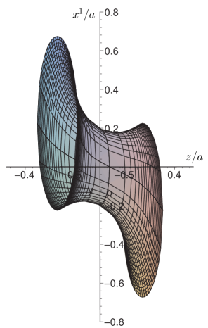
Figure 1: The trapped surface for $b=b_{max}=0.8045a$ at the moment of appearance $T=T_{min}(b_{max})=0.228a$ .

5 Trapped surface formation

The dependence (6) of $b/a$ on $ka$ (Fig. 2) shows that for a given $b$ there are two values of $k:k_{1}(b)<k_{2}(b)$ . The impact parameter $b$ reaches its maximum value $b_{max}=0.8047a$ at $k=1.98/a$. This limits a cross-section of a black hole production in a two shocks impact [3].

The trapped surface appears at $T=T_{min}$. For a given $b$ there are two values of $T_{min}:T_{min\,1}<T_{min\,2}$ corresponding to $k_{1}(b)$ and $k_{2}(b)$ respectively (Fig. 3). The relation between parameter $c$ and $T$ is also two-valued (Fig. 4).

On the whole, the process of the horizon formation looks as follows. The horizon appears at $T=T_{min\,1}$. At $T_{min\,1}<T<T_{min\,2}$ two trapped surfaces exist. One on them (internal) is located inside another one (external). Their evolution is illustrated in Fig. 5B, where ($x^{2}=0$)-sections of the trapped surfaces at different times are presented. As time $T$ increases ($z=0$)-diameter of the internal and external surfaces decreases and increases respectively. At $T=T_{min\,2}$ two other trapped surfaces appear with similar properties (Fig. 5A).

So, at $T>T_{min\,2}$ we have four different trap surfaces. The biggest one of them is the external surface that appears at $T=T_{min\,1}$. It may be considered as a horizon. Others are spaced inside it. It is possible that in more realistic model the number of the trapped surfaces will be less and the horizon may be defined more precisely.

According to the results of [5] where the head-on collision was investigated we may expect that the results obtained above may be qualitatively correct in higher dimensions.

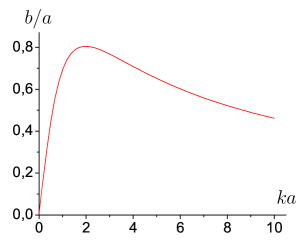
Figure 2: The dependence of $b/a$ on $ka$. $(b/a)_{max}=0.8047$ at $ka=1.9803$

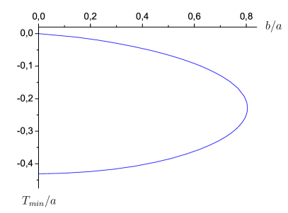
Figure 3: The dependence of $T_{min}/a$ on $b/a$ .

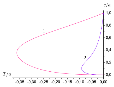
Figure 4: The dependences of $c/a$ on $T/a$ for $b/a=0.6$. 1 – $k_{1}=0.76$, 2 – $k_{2}=6.04$ .

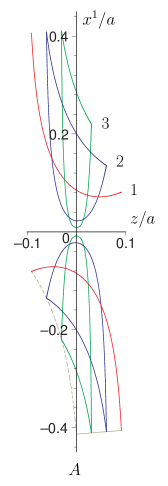
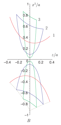
Figure 5: The ($x^{2}=0$)-sections of the trapped surfaces for $b=0.6$ at different times $T$. $A$ — $k_{2}=6.04,\ T_{min\,2}/a=-0.092$; $B$ — $k_{1}=0.76,\ T_{min\,2}/a=-0.362$ . 1 — $T=T_{min}$; 2 — $T=2T_{min}/3$; 3 — $T=T_{min}/3$. For $T>T_{min}$ there are external and internal surfaces corresponding to $c>c(T_{min)}$ and $c<c(T_{min})$ respectively (Fig.4). In the low parts of the graphics trajectories of endpoints are shown by dot lines.

References

[1] S. B. Giddings
“High-energy black hole production”,
arXiv:0709.1107 [hep-ph].
[2] P. Kanti,
“Black Holes at the LHC”, arXiv:0802.2218 [hep-th].
[3] D. M. Eardley and S. B. Giddings,
“Classical black hole production in high-energy
collisions”, arXiv:gr-qc/0201034.
[4]
H. Yoshino, Y. Nambu, “High-energy head-on collisions of
particles and hoop conjecture”, Phys.Rev. D 66 (2002)
065004 [arXiv:gr-qc/0204060].
[5] O. I. Vasilenko,
“Trap Surface Formation in High-Energy Black Holes
Collision”, arXiv:hep-th/0305067; Vestnik Moskovskogo
Universiteta. Fizika. Astronomia. 4, 42 (2004)
[6]
P. C. Aichelburg and R. U. Sexl, “On The Gravitational Field
Of A Massless Particle”, Gen. Rel. Grav. 2, 303
(1971).
[7]
T. Dray and G. ‘t Hooft, “The Gravitational Shock Wave of a
Massless Particle,” Nuclear Physics B 235, 173–188
(1985).
[8] R. Penrose, “Structure of Space-Time”,
in Battelle Rencontres (edit. by C. M. DeWitt and
J. A. Wheeler) (Benjamin, New York, 1968).
[9]
B. A. Dubrovin, S. P. Novikov, A. T. Fomenko, “Sovremennaya
geometriya”, Nauka, Moskva (1979); “Modern
Geometry-Methods and Applications, Part I: The Geometry of
Surfaces, Transformation Groups, and Fields”, Springer Verlag,
2-nd edition (January 1992).