${\cal N}=(1,1)$ super Yang–Mills theory in 1+1 dimensions at finite temperature

John R. Hiller

Department of Physics
University of Minnesota Duluth
Duluth MN 55812

Yiannis Proestos, Stephen Pinsky, and Nathan Salwen

Department of Physics
Ohio State University
Columbus OH 43210

We present a formulation of ${\cal N}=(1,1)$ super Yang–Mills theory in 1+1 dimensions at finite temperature. The partition function is constructed by finding a numerical approximation to the entire spectrum. We solve numerically for the spectrum using Supersymmetric Discrete Light-Cone Quantization (SDLCQ) in the large-$N_{c}$ approximation and calculate the density of states. We find that the density of states grows exponentially and the theory has a Hagedorn temperature, which we extract. We find that the Hagedorn temperature at infinite resolution is slightly less than one in units of $\sqrt{g^{2}N_{\rm c}/\pi}$. We use the density of states to also calculate a standard set of thermodynamic functions below the Hagedorn temperature. In this temperature range, we find that the thermodynamics is dominated by the massless states of the theory.

1 Introduction

In ${\cal N}=4$ super Yang–Mills theory at large $N_{c}$, there is a known mismatch between weak and strong coupling by a factor of 3/4 in the free energy [1]. The weak-coupling result is calculable in perturbation theory; the strong-coupling result comes from black-hole thermodynamics. It would be interesting to be able to directly solve this theory at all couplings and see the transition between the weak-coupling and strong-coupling limits [2]. Analytically this is generally not possible, although there have been a number of early discussions of methods for finite-temperature solutions to supersymmetric quantum field theory [3]. We will instead consider a numerical method based on Supersymmetric Discrete Light-Cone Quantization (SDLCQ) [4, 5], which preserves the supersymmetry exactly. Currently this is the only method available for numerically solving strongly coupled super Yang–Mills theories. Conventional lattice methods have difficulty with supersymmetric theories because of the asymmetric way that fermions and bosons are treated, and progress [6] in supersymmetric lattice gauge theory has been relatively slow.

Given that SDLCQ makes use of light-cone coordinates, with $x^{+}=(x^{0}+x^{3})/\sqrt{2}$ the time variable and $p^{-}=(p^{0}-p^{3})/\sqrt{2}$ the energy, we must take some care in defining thermodynamic quantities. The seemingly natural choice [7] of $e^{-\beta_{{}_{\rm LC}}p^{-}}$ as the partition function has been shown by Alves and Das [8] to lead to singular results for well known quantities that are finite in the equal-time approach. They argue that using $e^{-\beta_{{}_{\rm LC}}p^{-}}$ for the partition function implies that the physical system is in contact with a heat bath that has been boosted to the light-cone frame and that this is not equivalent to the physics of a system in contact with a heat bath at rest.

A more direct way to see this is that, since the light-cone momentum $p^{+}=(p^{0}+p^{3})/\sqrt{2}$ is conserved, the partition function must include it in the form $Z=e^{-\beta_{{}_{\rm LC}}(p^{-}+\mu p^{+})}$, with $\mu$ its chemical potential. The interpretation of the chemical potential is that of a rotation of the quantization axis. Thus $\mu=1$ corresponds to quantization in an equal-time frame, where the heat bath is at rest and the inverse temperature $\beta=\sqrt{2}\beta_{{}_{\rm LC}}$, and $\mu\neq 1$ corresponds to quantization in a boosted frame where the heat bath is not at rest. Thus $\mu$ corresponds to a continuous rotation of the axis of quantization, and $\mu=0$ would correspond to rotation all the way to the light-cone frame. A rotation from an equal-time frame to the light-cone frame is not a Lorentz transformation. It is known that such a transformation can give rise to singular results for physical quantities. This appears to be consistent with the results found in [8]. A number of related issues have been extensively discussed by Weldon [9]. The method has also recently been applied to the Nambu–Jona-Lasinio model [10].

These difficulties are avoided if we compute the equal-time partition function $Z=e^{-\beta p^{0}}$, as was proposed much earlier by Elser and Kalloniatis [11]. The computation may, of course, still use light-cone coordinates. Elser and Kalloniatis did this with ordinary DLCQ [12, 13] as the numerical approximation to (1+1)-dimensional quantum electrodynamics. Here we will follow a similar approach using SDLCQ to calculate the spectrum of ${\cal N}=(1,1)$ super Yang–Mills theory in 1+1 dimensions [14]. Though this calculation is done in 1+1 dimensions, it is known that SDLCQ can be extended in a straightforward manner to higher dimensions [15, 16, 17].

We have discussed the SDLCQ numerical method in a number of other places, and we will not present a detailed discussion of the method here; for a review, see [5]. For those familiar with DLCQ [12, 13], it suffices to say that SDLCQ is similar; both have discrete momenta and cutoffs in momentum space, $x^{-}\in[-L,L]$. In 1+1 dimensions the discretization is specified by a single integer $K=(L/\pi)P^{+}$, the resolution, such that longitudinal momentum fractions are integer multiples of $1/K$. However, SDLCQ is formulated in such a way that the theory is also exactly supersymmetric. Exact supersymmetry brings a number of very important numerical advantages to the method; in particular, theories with enough supersymmetry are finite. We have also seen greatly improved numerical convergence in this approach.

In Sec. 2 we briefly review super Yang–Mills theory in 1+1 dimensions. The discussion in Sec. 3 describes the method we use to extract the density of states from the numerical spectrum. The calculation of the density of states is presented in Sec. 4. We fit the data to smooth analytical functions, and we find that the theory has a Hagedorn temperature $T_{H}$ [18], which we calculate. In Sec. 5, we use the analytic fit to the density of states to calculate the free energy, the energy, and the specific heat, up to the Hagedorn temperature. Section 6 contains a discussion of our results and the prospects for future work using these methods.

2 Super Yang–Mills theory

We will start by providing a brief review of ${\cal N}=(1,1)$ supersymmetric Yang–Mills in 1+1 dimensions. The Lagrangian of this theory is

$${\cal L}={\rm Tr}\left(-\frac{1}{4}F_{\mu\nu}F^{\mu\nu}+i\bar{\Psi}\gamma_{\mu}D^{\mu}\Psi\right).$$ (1)

The two components of the spinor $\Psi=2^{-1/4}({\psi\atop\chi})$ are in the adjoint representation, and we will work in the large-$N_{c}$ limit. The field strength and the covariant derivative are $F_{\mu\nu}=\partial_{\mu}A_{\nu}-\partial_{\nu}A_{\mu}+ig[A_{\mu},A_{\nu}]$ and $D_{\mu}=\partial_{\mu}+ig[A_{\mu},~{}]$. The most straightforward way to formulate the theory in 1+1 dimensions is to start with the theory in 2+1 dimensions and then simply dimensionally reduce to 1+1 dimensions by setting $\phi=A_{2}$ and $\partial_{2}\rightarrow 0$ for all fields. In the light-cone gauge, $A^{+}=0$, we find

$$Q^{-}=2^{3/4}g\int dx^{-}{\rm Tr}\left(i[\phi,\partial_{-}\phi]\frac{1}{\partial_{-}}\psi+2\psi\psi\frac{1}{\partial_{-}}\psi\right).$$ (2)

The mode expansions in two dimensions are

$$\phi_{ij}(0,x^{-}) = \frac{1}{\sqrt{2\pi}}\int_{0}^{\infty}\frac{dk^{+}}{\sqrt{2k^{+}}}\left[a_{ij}(k^{+})e^{-{\rm i}k^{+}x^{-}}+a^{\dagger}_{ji}(k^{+})e^{{\rm i}k^{+}x^{-}}\right],$$

$$\psi_{ij}(0,x^{-}) = \frac{1}{2\sqrt{\pi}}\int_{0}^{\infty}dk^{+}\left[b_{ij}(k^{+})e^{-{\rm i}k^{+}x^{-}}+b^{\dagger}_{ji}(k^{+})e^{{\rm i}k^{+}x^{-}}\right].$$ (3)

To obtain the spectrum, we solve the mass eigenvalue problem

$$2P^{+}P^{-}|\varphi\rangle=\sqrt{2}P^{+}(Q^{-})^{2}|\varphi\rangle=M^{2}|\varphi\rangle.$$ (4)

This theory has two discrete symmetries, besides supersymmetry, that we use to reduce the size of the Hamiltonian matrix we have to calculate. $S$-symmetry, which is associated with the orientation of the large-$N_{c}$ string of partons in a state [19], gives a sign when the color indices are permuted

$$S:a_{ij}(k)\rightarrow-a_{ji}(k),\qquad b_{ij}(k)\rightarrow-b_{ji}(k).$$ (5)

$P$-symmetry is what remains of parity in the $x^{2}$ direction after dimensional reduction

$$P:a_{ij}(k)\rightarrow-a_{ij}(k),\qquad b_{ij}(k)\rightarrow b_{ij}(k).$$ (6)

All of our states can be labeled by the $P$ and $S$ sector in which they appear.

We convert the mass eigenvalue problem $2P^{+}P^{-}|M\rangle=M^{2}|M\rangle$ to a matrix eigenvalue problem by introducing a discrete basis where $P^{+}$ is diagonal. We will always state $M^{2}$ in units of $g^{2}N_{c}/\pi$. In SDLCQ the discrete basis is introduced by first discretizing the supercharge $Q^{-}$ and then constructing $P^{-}$ from the square of the supercharge: $P^{-}=(Q^{-})^{2}/\sqrt{2}$. To discretize the theory, we impose periodic boundary conditions on the boson and fermion fields alike and obtain an expansion of the fields with discrete momentum modes. We define the discrete longitudinal momenta $k^{+}$ as fractions $nP^{+}/K$ of the total longitudinal momentum $P^{+}$, where $K$ is an integer that determines the resolution of the discretization and is known in DLCQ as the harmonic resolution [12]. Because light-cone longitudinal momenta are always positive, $K$ and each $n$ are positive integers; the number of constituents is then bounded by $K$. The continuum limit is recovered by taking the limit $K\rightarrow\infty$.

In constructing the discrete approximation, we drop the longitudinal zero-momentum mode. For some discussion of dynamical and constrained zero modes, see the review [13] and previous work [20]. Inclusion of these modes would be ideal, but the techniques required to include them in a numerical calculation have proved to be difficult to develop, particularly because of nonlinearities. For DLCQ calculations that can be compared with exact solutions, the exclusion of zero modes does not affect the massive spectrum [13]. In scalar theories it has been known for some time that constrained zero modes can give rise to dynamical symmetry breaking [13], and work continues on the role of zero modes and near zero modes in these theories [21, 22, 23, 24, 25].

3 Density of states

The thermodynamic functions will be written as sums over the spectrum $\{M_{n}\}$ of the theory. The most convenient way to calculate such sums is to represent each sum as an integral over a density of states $\rho(M^{2})$,

$$\sum_{n=1}^{\infty}\rightarrow\int\rho(M^{2})dM^{2}.$$ (7)

From our numerical solutions we can approximate the density of states by a continuous function. The remaining integrals in the thermodynamic functions are then done by standard numerical integration techniques, which are fast and convenient.

We can look at the density for a series of increasing resolutions $K$ in the SDLCQ approximation and thereby discuss the convergence of the density in the limit $K\rightarrow\infty$. The maximum mass that we can reach in the SDLCQ approximation increases as we increase the resolution. We report results for $11\leq K\leq 17$.

Convenient functions to extract from the spectral data [26] are the cumulative distribution function (CDF) $N(M^{2},K)$ and the normalized cumulative distribution function (NCDF) $f(M^{2},K,M^{2}_{r})$. The CDF is the number of massive states at or below $M^{2}$ at resolution $K$, and the NCDF is this number divided by the total number of massive states below an arbitrary normalization point $M^{2}_{r}$, again at resolution $K$:

$$f(M^{2},K,M^{2}_{r})=\frac{N(M^{2},K)}{N(M^{2}_{r},K)}.$$ (8)

The function $f$ turns out to be very smooth and can be fit by a single smooth analytic form. By definition, the density of states is given by

$$\rho(M^{2},K)=\frac{dN\left(M^{2},K\right)}{dM^{2}}.$$ (9)

It is also convenient to define a normalized density of states [26]

$$\tilde{\rho}(M^{2},K,M^{2}_{r})=\frac{df\left(M^{2},K,M^{2}_{r}\right)}{dM^{2}}.$$ (10)

It is well known that if the density of states grows exponentially with the mass of the state,

$$\rho(M^{2})\sim{\rm{exp}}(M/T_{\rm{H}}),$$ (11)

the theory will have a Hagedorn temperature, $T_{\rm{H}}$ [18]. Above the temperature $T_{H}$, the thermodynamic integrals diverge.

4 Numerical results for the density of states

The numerical results presented in this section are the first from our new code, which was rewritten to run on clusters. Most of these results were produced on our six-processor development cluster. While this cluster was sufficient for this problem, we expect to be able to handle larger problems by moving to larger clusters. In fact, it is now so easy to generate the Hamiltonian up to resolution $K=17$, that we only used one node in our cluster for that purpose. What made this calculation challenging numerically was that we needed to extract a large number of eigenvalues. For the largest values of the resolution, this was done with a specially tuned Lanczos diagonalization code based on the techniques of Cullum and Willoughby [27]. We should note that, prior to the development of the new matrix-generation code, the highest resolution results presented for this theory were for resolution $K=10$ [14]. Here we will present only resolutions $K\geq 11$. All our earlier results are now trivially reproduced.

(a)	(b)

Figure 1: The distribution functions (a) $N(M^{2},K)$ for $K=12$ and (b) $f(M^{2},K,100)$ for $K=12$, 14, and 17, as functions of $M^{2}$ in units of $g^{2}N_{c}/\pi$. In (a) we also show the error-function fit $a\,{\rm erf}(b(x-c))+d$, and in (b), a polynomial fit.

In the SDLCQ approximation, the portion of the spectrum that we can see at any finite resolution will naturally be cut off. As we approach the cutoff, the approximation limits the number of states that are available and distorts the density of states. In Fig. 1a, we present the data for the CDF at resolution $K=12$, where we can diagonalize the entire Hamiltonian. We clearly see evidence of this distortion. By the midpoint, the cutoff is already diminishing the number of states available in the approximation. Interestingly, we can find a fit to this data with a simple universal function of the form $a\,{\rm erf}(b(x-c))+d$. Clearly the fit shown is excellent; the fit is so good that one cannot separately see the data and the fitted curve on this scale.

At low masses, there is a mass gap, which has been discussed elsewhere [5]. The mass gap closes linearly with $1/K$. For very small values of $M^{2}$, the decrease of the mass gap with increasing resolution adversely affects the quality of the universal fit, and it is convenient in that region to improve the quality of the fit by using a polynomial function of the form

$$f(x,K,100)=\sum_{p=0}^{p(K)}\alpha_{p}\,x^{\delta_{K}+p}\Theta(x-x_{\rm min}(K)).$$ (12)

In Fig. 1b we show the fit to the NCDF for some representative values of the resolution $K$. We have only shown the data at resolutions $K=12$, 14, and 17 to keep the figure uncluttered. One can see how the endpoints tend to lower values as the mass gap closes with increasing $K$.

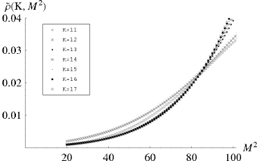
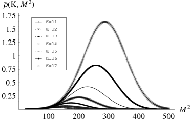
(a)	(b)

Figure 2: The normalized density of states (a) for $M^{2}\leq 100$ and (b) extrapolated to all masses. The data points are a convenient way of displaying the continuous functions calculated from the fits to the CDF.

At larger values of $K$ it is difficult to completely diagonalize the entire Hamiltonian. We have limited ourselves to states with $M^{2}\leq 100$. However, once we know the universal form of the function that fits the CDF, we can fit just the region $M^{2}\leq 100$ and extrapolate to all masses. At large $M^{2}$, the CDF approaches the total number of bound states. The total number of states in the SDLCQ approximation at any resolution, and, in any symmetry sector in the large-$N_{c}$ approximation, is exactly calculable; the general results will be discussed elsewhere. We use this asymptotic value of the CDF, in addition to the behavior for $M^{2}\leq 100$, in making the fits. We have done this at all resolutions up to $K=17$. In Fig. 2a we show the normalized density of states calculated from the NCDF, for $M^{2}\leq 100$. In Fig. 2b we show the normalized density of states for $11\leq K\leq 17$, extrapolated to the full range of masses.

(a)	(b)

Figure 3: The Hagedorn temperature $T_{H}$, as obtained from exponential fits, $\alpha\,{\rm{exp}}\left(\frac{M}{T_{\rm H}}\right)-\alpha$, to the universal fits to $N(M^{2},K)$, as shown in (a) for $K=17$, and (b) a linear plot against $1/K$ for fits in the range $11\leq K\leq 17$.

Inspecting these curves, we see that on the up-slope part of the density of states, where we believe our numerical approximation is a valid approximation to the actual density of states, the shape appears exponential. As we go to larger and larger values of the resolution $K$, the size of this region grows. This suggests that the density of states ultimately becomes simply an exponential, and, therefore, this theory has a Hagedorn temperature. To find the Hagedorn temperature, we fit the NCDF in this up-slope region with a function of the form

$$f(M^{2},K,100)=\alpha\,{\rm{exp}}\left(\frac{M}{T_{\rm H}}\right)-\alpha.$$ (13)

In Fig. 3b we plot $T_{H}$ against $1/K$. This yields a good linear fit, which we extrapolate to infinite resolution. We find that the Hagedorn temperature at infinite resolution is slightly less than one in units of $\sqrt{g^{2}N_{\rm c}/\pi}$. This value serves as a limiting temperature for the region of validity in the calculation of thermodynamic quantities.

5 Finite temperature in 1+1 dimensions

In the large-$N_{c}$ approximation, the numerical solution of a theory is a set of non-interacting bound states. Therefore, the thermodynamics of such supersymmetric theories is simply the thermodynamics of a gas of a large number of species of degenerate bosons and fermions. In principle, one could go beyond the calculation of the standard set of the thermodynamic functions and calculate a variety of matrix elements. These calculations would require the wave functions of the bound states, which can be calculated as part of the SDLCQ calculation. We will, however, not exploit this detailed information here. We will focus on the calculation of standard thermodynamic quantities that can be obtained from the density of states. The light cone plays no role beyond the calculation of the density; the thermodynamics is that of a system at rest.

Let us now briefly review the thermodynamics of free bosons and fermions. We assume that our system has constant volume $V$ and is in contact with a heat bath of constant temperature $T$. The free energy in units with $k_{B}=1$ is

$${\cal{F}}(T,V)=-T\ln Z.$$ (14)

The contribution of a single bosonic oscillator to the free energy $F_{B}$ is

$$F_{B}=2VT\int_{0}^{\infty}{\frac{dp_{3}}{2\pi}{\ln{\left(1-e^{-p_{0}/T}\right)}}},$$ (15)

where $p_{0}=\sqrt{M^{2}+p_{3}^{2}}$ and the factor of 2 compensates for integrating over only positive values of $p_{3}$. It is convenient to change variables from $p_{3}$ to $p_{0}$:

$$dp_{3}=\frac{p_{0}}{\sqrt{p_{0}^{2}-M^{2}}}dp_{0}.$$ (16)

The limits of integration are changed from $0\leq p_{3}<\infty$ to $M\leq p_{0}<\infty$. We may also use the following representation for the logarithm that appears in the integrand

$${\ln{\left(1-e^{-p_{0}/T}\right)}}=-\sum_{j=1}^{\infty}\frac{e^{-jp_{0}/T}}{j},$$ (17)

since $p_{0}$ is positive and $0\leq e^{-p_{0}/T}<1$. Finally, we obtain an expression for the total bosonic free energy just by summing over the energy spectrum

$${\cal{F}}_{B}=-\frac{VT}{\pi}\sum_{n=1}^{\infty}{\sum_{j=1}^{\infty}}\int_{M_{n}}^{\infty}{dp_{0}\frac{p_{0}}{\sqrt{p_{0}^{2}-M_{n}^{2}}}{\left(\frac{e^{-jp_{0}/T}}{j}\right)}}.$$ (18)

The calculation of the fermionic contribution to the free energy proceeds analogously, and we find the identical result with the exception that there is a factor of $(-1)^{j}$ inside the summation. We can separate out the massless states from these expressions and calculate their contribution explicitly. We know that for resolution $K$ there are $(K-1)$ massless bosons and $(K-1)$ massless fermions. Thus the contribution to the free energy from massless states is

$${\cal{F}}^{0}_{B}=-\frac{(K-1)\pi}{6}VT^{2},\quad{\cal{F}}^{0}_{F}=-\frac{(K-1)\pi}{12}VT^{2}.$$ (19)

After doing the integral over $p_{0}$, we find for the total free energy

$$\frac{{\cal{F}}(T,V)}{VT^{2}}=-\frac{(K-1)\pi}{4}-\frac{2}{T\pi}\sum_{n=1}^{\infty}{\sum_{l=0}^{\infty}}M_{n}\frac{K_{1}\left((2l+1)\frac{M_{n}}{T}\right)}{(2l+1)}.$$ (20)

The even terms, where $j=2l$ in the original sum, cancel between the fermion and boson contributions. We have also factored out the temperature dependence of the massless contribution and the volume dependence.

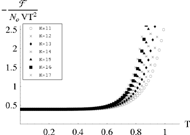
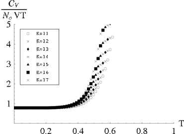
(a)	(b)

Figure 4: The free energy (a) and the heat capacity (b) as functions of temperature for each resolution. Both functions are normalized to the number of massless states, $N_{0}=2(K-1)$. The data points are a convenient way to display the continuous functions calculated from fits to the CDF.

We can now rewrite the free energy in terms of the density of states. The sums involving the Bessel function are cut off at a few terms; generally $l_{\rm cut}\leq 2$ will be sufficient. We find

$$\frac{{\cal F}(T,V)}{VT^{2}}=-\frac{(K-1)\pi}{4}-\frac{2}{\pi T}\int_{M_{\rm min}^{2}}^{\infty}dM^{2}\rho(M^{2})M\sum_{l=0}^{l_{\rm cut}}\frac{K_{1}\left((2l+1)\frac{M}{T}\right)}{(2l+1)}.$$ (21)

The free energy may now be used to calculate all the thermodynamic functions. The internal energy and heat capacity are given by,

$${\cal E}(T,V)=T^{2}\left(\frac{\partial{\ln Z}}{\partial{T}}\right)_{\rm V},\quad{\cal C}_{\rm V}(T,V)=\left(\frac{\partial{{\cal E}}}{\partial{T}}\right)_{\rm V}.$$ (22)

It is straightforward, given the density of states, to calculate the thermodynamic functions. Fig. 4a shows the free energy, and Fig. 4b shows the heat capacity. We expect the free energy to diverge as $N_{c}^{2}$ and therefore must normalize our results to extract a finite number. In most of the region below the Hagedorn temperature the thermodynamic functions are totally dominated by the massless states. It therefore seems appropriate to normalize the thermodynamic functions to the total number of massless bound states, which is a function of the resolution and is $2(K-1)$. Alternatively, we could normalize by the number of states in any region. It is conceivable that at very high resolutions, where the mass gap is significantly less than one, that the massive states may make an important contribution to the thermodynamics. In that case we would not choose to normalize by the massless states.

6 Discussion

The large-$N_{c}$ SDLCQ solution of ${\cal N}=(1,1)$ super Yang–Mills theory in 1+1 dimensions gives a set of non-interacting bound states. From this set of bound states it is in principle possible to calculate the thermodynamics of this theory. Central to this calculation is the calculation of the density of states. At resolutions $K=12$ and below, where we can completely diagonalize the Hamiltonian, we find that the entire cumulative distribution function can be fit with a single erf function. From the cumulative distribution function, it is straightforward to calculate the density of states. For $K$ larger than 12, it is difficult to calculate the entire spectrum; therefore, our calculations are confined to a fixed range of masses, $M^{2}\leq 100\,g^{2}N_{c}/\pi$. Using the known form of the distribution, we only need to fit a section of the cumulative distribution function to get a very good fit to the entire distribution. We know analytically the total number of bound states at any resolution, and this information can also be used in conjunction with a fit to a section of the distribution to produce the fit to the entire distribution.

The density of states that are found by this procedure grow sharply at small masses, then level off and decrease at larger masses. The peak of the density of states grows as we increase the resolution. Our understanding of this behavior is that the cutoff of the theory is forcing the density of states to level off, turn over, and then decrease. The true behavior of the density of states is reflected in the region of the density of states that is rapidly increasing, because it is this region that is increasing in size with the resolution $K$.

It appears that the cumulative distribution function, and, therefore, the density of states, are growing exponentially with the mass. To confirm this and find the asymptotic values of this growth, we fit the cumulative distribution function with an exponential at each $K$. We extrapolate these results to infinite resolution to find the asymptotic behavior of the density of states. The coefficient of the exponential growth is the reciprocal of the Hagedorn temperature. We find that this temperature is about $0.854\,\sqrt{g^{2}N_{c}/\pi}/k_{B}$. The thermodynamic functions calculated from this data are expected to produce valid results up to a temperature that is around $T_{\rm H}$.

It is now straightforward to calculate a standard set of thermodynamic functions from this density of states. The best estimate of the thermodynamics is obtained by using the exponential fits to the density of states. What we see is that, for resolutions up to $K=17$, all of the massive bound states are well above the Hagedorn temperature. The thermodynamics below $T_{H}$ is therefore controlled by the $K-1$ massless boson bound states and $K-1$ massless fermion bound states.

We can speculate on what will happen as the resolution goes to infinity. We have seen that the mass gap closes linearly with $1/K$. So, for a resolution of order 100, there will be massive bound states below the Hagedorn temperature. This, of course, assumes that the estimate of the Hagedorn temperature is not changed by the higher resolution calculations. We found, however, that the actual number of massive bound states in a fixed mass range may grow slowly. For resolutions 11 to 17 we are able to find excellent fits with both exponential and linear growth as a function of the resolution $K$ for masses with $M^{2}\leq 100$. If the number of massive states grows only linearly with $K$, the contribution to the thermodynamic functions below $T_{H}$ might become significant but not dominant.

These calculations indicate that ${\cal N}=(1,1)$ super Yang–Mills theory in 1+1 dimensions has a Hagedorn temperature of about one in units of $\sqrt{g^{2}N_{c}/\pi}/k_{B}$. More generally, we found that SDLCQ can be used to find interesting properties of finite-temperature supersymmetric field theories. The extension of this method to theories with more supersymmetry and in higher dimensions appears to be straightforward but may be computationally challenging.

References

- [1] S. S. Gubser, I. R. Klebanov, and A. W. Peet, Phys. Rev. D 54, 3915 (1996) [arXiv:hep-th/9602135].
- [2] M. Li, JHEP 9903, 004 (1999) [arXiv:hep-th/9807196]; A.A. Tseytlin and S. Yankielowicz, D3-brane Nucl. Phys. B 541, 145-162 (1999) [arXiv:hep-th/9809032]; A. Fotopoulos and T.R. Taylor, at finite temperature,” Phys. Rev. D 59, 061701 (1999) [arXiv:hep-th/9811224].
- [3] A. Das and M. Kaku, Phys. Rev. D 18, 4540 (1978).
- [4] Y. Matsumura, N. Sakai, and T. Sakai, Phys. Rev. D 52, 2446 (1995) [arXiv:hep-th/9504150].
- [5] O. Lunin and S. Pinsky, AIP Conf. Proc. 494, 140 (1999) [arXiv:hep-th/9910222].
- [6] A. G. Cohen, D. B. Kaplan, E. Katz, and M. Unsal, [arXiv:hep-lat/0302017]; A. Feo, to appear in the proceedings of the 20th International Symposium on Lattice Field Theory (LATTICE 2002), Boston, Massachusetts, 24-29 Jun 2002, [arXiv:hep-lat/0210015]; I. Montvay, Nucl. Phys. B 466, 259 (1996) [arXiv:hep-lat/9510042].
- [7] S. J. Brodsky, Nucl. Phys. Proc. Suppl. 108, 327 (2002) [arXiv:hep-ph/0112309].
- [8] V. S. Alves, A. Das, and S. Perez, Phys. Rev. D 66, 125008 (2002) [arXiv:hep-th/0209036]; A. Das and X. X. Zhou, Phys. Rev. D 68, 065017 (2003) [arXiv:hep-th/0305097]; A. Das, arXiv:hep-th/0310247.
- [9] H. A. Weldon, Phys. Rev. D 26, 1394 (1982); 67, 085027 (2003) [arXiv:hep-ph/0302147]; 67, 128701 (2003) [arXiv:hep-ph/0304096].
- [10] M. Beyer, S. Mattiello, T. Frederico, and H. J. Weber, [arXiv:hep-ph/0310222].
- [11] S. Elser and A. C. Kalloniatis, Phys. Lett. B 375, 285 (1996) [arXiv:hep-th/9601045].
- [12] H.-C. Pauli and S.J. Brodsky, Phys. Rev. D 32, 1993 (1985); 32, 2001 (1985);
- [13] S.J. Brodsky, H.-C. Pauli, and S.S. Pinsky, Phys. Rep. 301, 299 (1998) [arXiv:hep-ph/9705477].
- [14] F. Antonuccio, O. Lunin, and S. S. Pinsky, Phys. Lett. B 429, 327 (1998) [arXiv:hep-th/9803027]. F. Antonuccio, O. Lunin, and S. Pinsky, Phys. Rev. D 58, 085009 (1998) [arXiv:hep-th/9803170].
- [15] F. Antonuccio, O. Lunin, and S. Pinsky, Phys. Rev. D 59, 085001 (1999) [arXiv:hep-th/9811083].
- [16] P. Haney, J. R. Hiller, O. Lunin, S. Pinsky, and U. Trittmann, Phys. Rev. D 62, 075002 (2000) [arXiv:hep-th/9911243].
- [17] J. R. Hiller, S. Pinsky, and U. Trittmann, Phys. Rev. D 64, 105027 (2001) [arXiv:hep-th/0106193].
- [18] R. Hagedorn, Nuovo Cimento Suppl. 3, 147 (1965); R. Hagedorn, Nuovo Cimento 56A, 1027 (1968).
- [19] D. Kutasov, Phys. Rev. D48, 4980 (1993) [arXiv:hep–th/9306013].
- [20] F. Antonuccio, O. Lunin, S. Pinsky, and S. Tsujimaru, Phys. Rev. D 60, 115006 (1999) [arXiv:hep-th/9811254].
- [21] J. S. Rozowsky and C. B. Thorn, Phys. Rev. Lett. 85, 1614 (2000) [arXiv:hep-th/0003301].
- [22] S. Salmons, P. Grange, and E. Werner, Phys. Rev. D 65, 125014 (2002) [arXiv:hep-th/0202081].
- [23] T. Heinzl, arXiv:hep-th/0310165.
- [24] A. Harindranath, L. Martinovic, and J. P. Vary, Phys. Lett. B 536, 250 (2002); V. T. Kim, G. B. Pivovarov, and J. P. Vary, Phys. Rev. D 69, 085008 (2004) [arXiv:hep-th/0310216].
- [25] D. Chakrabarti, A. Harindranath, L. Martinovic, and J. P. Vary, Phys. Lett. B 582, 196 (2004) [arXiv:hep-th/0309263].
- [26] O. Lunin and S. Pinsky, Phys. Rev. D 63, 045019 (2001) [arXiv:hep-th/0005282].
- [27] J. Cullum and R.A. Willoughby, in Large-Scale Eigenvalue Problems, eds. J. Cullum and R.A. Willoughby, Math. Stud. 127 (Elsevier, Amsterdam, 1986), p. 193.