On Localized Tachyon Condensation in $\mathbb{C}^{2}/\mathbb{Z}_{n}$ and $\mathbb{C}^{3}/\mathbb{Z}_{n}$

1 Introduction

In recent years, the issue of tachyon condensation on unstable backgrounds has been studied extensively in string theory, and has led to a number of useful insights. In open string theory, this problem has been investigated by using various techniques, such as the boundary state formalism and boundary string field theory, following the pioneering work of Sen [1]. Tachyon condensation in closed string theory was first studied by Adams, Polchinski and Silverstein (APS) in [3], and subsequently in [4],[5], using different tools.

Whereas open string tachyon condensation typically involves a change in the D-brane configuration of the system, the corresponding situation in the case of closed strings is very different. In general, condensation of closed string tachyons leads to a decay of the space-time itself. This can be difficult to study in general in the presence of bulk tachyons, but the situation is considerably simplified if the tachyons are localized on defects, such as orbifolds. The presence of tachyons will generically break space-time supersymmetry, but a lot of information can still be obtained by using world sheet RG flow methods.

The problem originally considered in [3] was string theory in the background of $\mathbb{R}^{1,7}\times\mathbb{C}/\mathbb{Z}_{n}$. This is the well known conical singularity with a deficit angle related to $n$. In this case, demanding that all the tachyonic modes are localized at the orbifold fixed point requires that $n$ is odd. It was shown in [3] that the $\mathbb{C}/\mathbb{Z}_{n}$ orbifold decays with time, i.e the original background decays into orbifolds of lower rank, and this process continues till we finally reach flat space-time. In terms of the conical geometry, this implies that the tip of the cone smooths out, and at the end of the decay we are left with flat space.

The situation is more complicated for higher dimensional singularities. Whereas for the $\mathbb{C}/\mathbb{Z}_{n}$ singularities, as we will discuss in a while, analysis of the conformal field theory (CFT) of the string world sheet shows that all the twisted sectors of the theory are tachyonic (i.e all the twist operators give rise to tachyons in space-time), for $\mathbb{C}^{2}/\mathbb{Z}_{n}$ orbifolds, certain twisted sectors might be marginal, and the theory can decay via the excitation of marginal deformations. Further, the decay process for these orbifolds stop once the system reaches a supersymmetric configuration, unlike the one-dimensional case, where the unique endpoint of tachyon condensation is flat space-time. Also, in certain examples, one finds that the $\mathbb{C}^{2}/\mathbb{Z}_{n}$ singularity may decay into a lower dimensional orbifold of the form $\mathbb{C}/\mathbb{Z}_{m}$. Expectedly, closed string tachyon condensation on non-supersymmetric orbifolds of the form $\mathbb{C}^{3}/\mathbb{Z}_{n}$ has an even richer structure [6], since the resolution of these singularities is not canonical, unlike the lower dimensional examples. It has been shown that in this case the endpoint of tachyon condensation may include terminal singularities.

We should also mention that the physics of tachyon condensation has contributed importantly to the understanding of some deep mathematical results on the resolution of singularities in complex two and three-fold orbifolds. In the mathematics literature, there exists a beautiful correspondence between the K-theory of the resolution of these orbifolds and the representation theory of the orbifolding group. This is known as the McKay correspondence, and it has been well known from the study of supersymmetric orbifolds that D-branes provide a physical realisation of this correspondence, in terms of branes wrapping cycles of the resolved singularity. It turns out that closed string tachyon condensation provides a way to understand a quantum version of the McKay correspondence [7], [8].

Much of the physics of closed string tachyon condensation can be captured by studying the worldsheet Gauged Linear Sigma Model (GLSM) of Witten [9] with non-supersymmetric orbifold backgrounds. This model, which we will describe in details in the course of the paper is also intimately related to toric constructions of these orbifolds [10].

Although much has been done in the above context, there are certain issues that still need to be explored. For example, consider the fact that the world sheet CFT description of orbifolds has a product structure, i.e various operators in higher dimensional theories can be constructed by simply combining lower dimensional ones. We see a reflection of this fact in the GLSM and toric constructions. One might expect that the GLSM corresponding to a supersymmetric orbifold of $\mathbb{C}^{3}$ can be obtained by adding an appropriate field to that corresponding to a non-supersymmetric $\mathbb{C}^{2}$ orbifold, and conversely, removing (i.e giving a vev) to certain fields in the GLSM might result in a lower dimensional orbifold. It is natural to ask whether this feature is more generic, i.e if higher dimensional orbifold theories can be thought of as certain combinations of lower dimensional ones. It turns out that this is indeed the case, and certain constructions of $\mathbb{C}^{3}$ orbifolds by a suitable combination of $\mathbb{C}^{2}$ orbifolds has already been performed in [11]. Although this has been constructed from the point of view of obtaining a crepant resolution to complex three-fold orbifolds, it might nevertheless be useful for our purposes, i.e for understanding closed string tachyon condensation in higher dimensional orbifolds in terms of lower dimensional ones.

In this paper, we set out to understand certain issues relating to the decay of non-supersymmetric orbifolds in lines with the above discussion. Our aim would be to extend and further develop certain ideas explored in [4],[7] in order to gain a better understanding of such decays. Further, we would explore the idea of studying the decay of higher dimensional orbifolds in terms of lower dimensional ones.

The paper is organised as follows. Section 2 is a review section, meant to set the notations and conventions used in the remainder of the paper. In section 3, we begin with the GLSM method of studying the fate of non-supersymmetric orbifolds by exploring background sigma model metrics of these models for orbifolds of $\mathbb{C}^{2}$ and $\mathbb{C}^{3}$ (this method has been employed in studying the decay of $\mathbb{C}/\mathbb{Z}_{n}$ in [12]). Section 4 deals with the understanding of certain field theory aspects of the GLSM for unstable backgrounds, using the methods of [4]. In section 5, we turn to toric geometry methods of studying the same, and then develop upon the idea of studying flows of $\mathbb{C}^{3}/\mathbb{Z}_{n}$ orbifolds in terms of orbifolds of $\mathbb{C}^{2}$. We conclude the paper with section 6, by summarising our results, and suggesting some future directions.

While this paper was being completed, reference [6] appeared, which has considered localized tachyon condensation on $\mathbb{C}^{3}/\mathbb{Z}_{n}$ orbifolds, and we have attempted to reconcile our results with theirs, wherever applicable.

2 Closed String Tachyon condensation on $\mathbb{C}^{r}/\mathbb{Z}_{n}$

In this section, we review some known facts about closed string tachyon condensation on orbifolds of the form $\mathbb{C}^{r}/\mathbb{Z}_{n}$, in order to set the notation and conventions used in the rest of the paper. For this purpose, we will mostly deal with the $\mathbb{C}/\mathbb{Z}_{n}$ and $\mathbb{C}^{2}/\mathbb{Z}_{n}$ orbifolds. We will come back to the case $r=3$ in details later in the paper. All the material of this section can be found in [3],[5], [4],[7],[10].

2.1 Review of the APS method

String theory in the background of orbifold singularities of the form $\mathbb{C}^{r}/\mathbb{Z}_{n}$ can be studied in various ways. In the sub-stringy regime, we expect the world volume gauge theory of D-branes probing these orbifolds to be an useful tool in the study. Indeed, by constructing the world volume gauge theories on D-p branes probing these orbifolds a’la Douglas and Moore [13], we can get very useful insights into the geometry of the resolutions, which in turn have descriptions in terms of certain toric varieties for $r>1$ . This is an open string description; an equivalent closed string picture of these orbifold singularities can be obtained in terms of the closed string world sheet super conformal field theory (SCFT) which enjoys $N=(2,2)$ worldsheet supersymmetry. By studying the twisted sectors of these SCFTs, we can read off the geometrical structure of the singularity.

Let us begin by describing string theory on $\mathbb{R}^{7,1}\times\mathbb{C}/\mathbb{Z}_{n}$ where $\mathbb{R}^{7,1}$ denotes eight dimensional Minkowski space labelled by $\left(X^{0},\cdots X^{7}\right)$, and the quotienting group acts on the complexified direction $Z=X^{8}+iX^{9}$ by the action

$$Z\to\omega Z$$ (1)

where $\omega=\mbox{e}^{\frac{2\pi i}{n}}$. This orbifold action breaks space-time supersymmetry, and introduces tachyons in all the twisted sectors of the orbifold conformal field theory. In order to have the tachyons localized at the fixed point of this orbifold we require $n$ to be odd for type II string theories [3]. If we consider a D-p brane probe of this singularity where the brane is located at the orbifold fixed point and the world volume directions are entirely in the transverse space, we can, following [13], construct the world volume gauge theory on the brane, by considering the action of $\mathbb{Z}_{n}$ on the world volume fields, and retaining those fields that are invariant under the action of the group. In this way, we obtain a quiver gauge theory of the massless world volume scalars. By giving vaccum expectation values (vevs) to certain scalars in the theory, we can determine (by examining the classical potential for the scalars) those scalars that become massive in the process (and hence can be integrated out), thus resulting in the quiver gauge theory of a lower rank orbifold [3]. The fermionic quivers can also be determined in a similar way by studying the Yukawa terms in the gauge theory. This construction is valid at substringy regimes, and far from this regime, when gravity effects become large, one has to resort to a full supergravity analysis. APS showed that these two regimes together give a consistent picture of the conical singularity decaying into flat space-time.

A similar analysis can be done for the complex two-dimensional orbifold, by considering string theory in the background of $\mathbb{R}^{5,1}\times\mathbb{C}^{2}/\mathbb{Z}_{n}$, where $\mathbb{R}^{5,1}$ is flat Minkowski space of six dimensions, labelled by the coordinates $X^{0},\cdots X^{5}$, and the orbifolding group acts on the complexified directions denoted by $Z^{1}=X^{6}+iX^{7}$ and $Z^{2}=X^{8}+iX^{9}$ as

$$\left(Z^{1},Z^{2}\right)\to\left(\omega Z^{1},\omega^{k}Z^{2}\right)$$ (2)

where $\omega=\mbox{e}^{\frac{2\pi i}{n}}$. When $k\neq\pm 1$, this action breaks space-time supersymmetry, and the orbifold is generically denoted by $\mathbb{C}^{2}/\mathbb{Z}_{n(k)}$. In this case, it is difficult to classify the flows by implementing the tachyonic vevs directly, as in the $\mathbb{C}/\mathbb{Z}_{n}$ example. The APS procedure here is to generate vevs for the fields in the theory in such a way as to maintain a certain quantum symmetry of the initial orbifolding group. This corresponds to the turning on of an appropriate (marginal) deformation in the CFT which breaks the other part of the group action. As in the $\mathbb{C}/\mathbb{Z}_{n}$ examples, one can analyse the classical substringy regime by resorting to brane probe techniques, and study the decay of these singularities, via the quiver gauge theories on the world volume of the probe branes. The gauge theory can be seen to give rise to the toric data for the resolution of the orbifold, as in the supersymmetric cases.

As an example, let us consider type II string theory in the background of the non-supersymmetric orbifold $\mathbb{C}^{2}/\mathbb{Z}_{8(3)}$. The action of the quotienting group is

$$\left(Z^{1},Z^{2}\right)\to\left(\omega Z^{1},\omega^{3}Z^{2}\right)$$ (3)

where $\omega=\mbox{e}^{\frac{2\pi i}{8}}$. This orbifold has seven twisted sectors of which the fourth twisted sector is marginal. By working out the discrete group action on the world-volume scalars, and retaining those fields that are invariant under this action, we find that the world volume gauge theory of a D-brane probing this orbifold has sixteen surviving components, charged under the $U(1)^{8}$ gauge group. The APS procedure is then to give vevs to a subset of these fields so as to maintain a certain quantum $U(1)^{4}$ symmetry, the vevs breaking the other part of the gauge group. This corresponds to the turning on of the marginal deformation corresponding to the fourth twisted sector of the orbifold CFT. These vevs can be turned on either via the surviving components of $Z^{1}$ or those of $Z^{2}$, and there are two distinct configurations into which the original theory can decay into. In this case, it turns out that the decay products obtained by turning on the said marginal deformation is [3]

$$\mathbb{C}^{2}/\mathbb{Z}_{8(3)}\to\mathbb{C}^{2}/\mathbb{Z}_{4(1)}\oplus\mathbb{C}^{2}/\mathbb{Z}_{4(1)}$$ (4)

The r.h.s of the above equation corresponds to two (infinitely separated) orbifolds that are supersymmetric with the opposite supersymmetry (i.e a change of complex structure makes the theory supersymmetric) compared to the usual supersymmetric $\mathbb{C}^{2}/\mathbb{Z}_{4(-1)}$ orbifold. If we choose one particular complex structure, these will be non-supersymmetric orbifolds that will further decay into flat space. In general, when the decay products are themselves non-supersymmetric, we can turn on further perturbations, marginal or tachyonic, in order to reach a final supersymmetric configuration, which might be flat space or a supersymmetric orbifold of lower rank.

Tachyon condensation in orbifolds of the form $\mathbb{C}^{3}/\mathbb{Z}_{n}$ can be similarly considered, and has a richer structure than the lower dimensional examples [6]. The orbifold action in this case is given by

$$\left(Z^{1},Z^{2},Z^{3}\right)\to\left(\omega Z^{1},\omega^{p_{1}}Z^{2},\omega^{p_{2}}Z^{3}\right)$$ (5)

where, like before, the $Z^{i}$s are the orbifolded directions and the transverse space is now four-dimensional. As explained in [6], the situation here is more subtle, since there is no canonical resolution of orbifolds of $\mathbb{C}^{3}$, and the decay process depends crucially on the condensation of the most relevant tachyon, i.e the tachyon with the highest negative mass squared. We will come back in details to three-fold orbifolds later in the paper.

We now move on to the description of these orbifolds in terms of the world sheet CFT of closed strings, which is intimately related to the toric geometry of the resolution of these singularities.

2.2 World Sheet CFT Analysis

In most cases, an equivalent picture of the APS description of the decay of unstable non-supersymmetric orbifolds can be obtained by examining the world sheet orbifold conformal field theory of closed strings, which in turn is related to methods of toric geometry in two and three (complex) dimensions. Let us begin with the orbifold $\mathbb{C}/\mathbb{Z}_{n}$. We will deal with type 0 theory here, with the delocalised untwisted sector tachyon tuned to zero. In the NSR formalism, we are dealing with a single world sheet chiral superfield $\Phi$ (which corresponds to the coordinate $\mathbb{C}$), and the orbifold action is $\Phi\to\omega\Phi$, with $\omega$ being the n-th root of unity. There are $(n-1)$ twisted sectors, and we can construct [16],[5] the twist operators

$$Y_{j}=\sigma_{j/n}{\mbox{exp}}\left[i\left(\frac{j}{n}\right)\left(H-{\bar{H}}\right)\right]$$ (6)

where $\sigma_{j/n}$ is the bosonic twist-j operator and $H$ and ${\bar{H}}$ denote the bosonised fermions. The operators in (6) are chiral, with R-charges $\frac{j}{n}$ in the $j$th twisted sector, and give rise to tachyons in space-time, with masses [5]

$$\frac{\alpha^{\prime}}{4}M_{j}^{2}=-\frac{1}{2}\left(1-\frac{j}{n}\right)$$ (7)

Note that the most tachyonic sector is, in this case, the first twisted sector, with the least R-charge, and the absolute value of the mass squared of the tachyon is proportional to the deficit angle of the conical singularity which this orbifold represents.

The decay of this orbifold is studied by perturbing the worldsheet Lagrangian by the vertex operators (6) with appropriate couplings, and studying the deformation of the chiral ring of the CFT due to this perturbation.

Higher (complex) dimensional orbifolds can also be studied in the same way. Here, the geometrical structure is richer, and in particular the CFT methods correspond nicely to tools of toric geometry used to study the resolution of these orbifold. Consider the orbifold $\mathbb{C}^{2}/\mathbb{Z}_{n}$. The twisted sector chiral operators are, in this case, given by combining the twist fields $Y^{(1)}$ and $Y^{(2)}$ of (6) corresponding to the two complexified directions as,

$$Y_{j}=Y_{\frac{j}{n}}^{(1)}Y_{\{\frac{jp}{n}\}}^{(2)}$$ (8)

where $j=1,\cdots(n-1)$ corresponds to the $(n-1)$ twisted sectors in the theory, and $\{x\}$ denotes the fractional part of the real number $x$ (the integral part of the real number $x$ is denoted by $\left[x\right]$). Orbifolds of this form have a convenient description in terms of toric geometry, via the Hirzebruch-Jung continued fraction.

In general, for orbifolds of the form $\mathbb{C}^{2}/\mathbb{Z}_{n(k)}$, where $k\neq n-1$, the resolution of the singularity can be succinctly described by the Hirzebruch-Jung continued function,

$$\frac{n}{k}=a_{1}-\frac{1}{a_{2}-\frac{1}{a_{3}-\frac{1}{...\frac{1}{a_{r}}}}}$$ (9)

where $a_{i}$ are integers, $a_{i}\geq 2$. The number of these integers $r$ determines the number of $\mathbb{P}^{1}$s that need to be blown up in order to resolve the singularity completely, and the integers $a_{i}$ determine the self intersection numbers of these $\mathbb{P}^{1}$s. These singularities are described in toric geometry by a data matrix that consists of a set of points in a two dimensional $SL(2,\mathbb{Z})$ lattice, and is of the form

$${\cal T}=\pmatrix{v_{0},v_{1}&v_{2}&v_{3}&...&v_{r+1}\cr}$$ (10)

where the interior vectors $v_{i},~{}i=1,\cdots,r$ satisfy the relation

$$a_{i}v_{i}=v_{i-1}+v_{i+1}$$ (11)

where $v_{0}=(0,-1),~{}v_{r+1}=(n,-k)$, and the $a_{i}$s are determined from the continued fraction (9). Equivalently, the toric data can be constructed following the prescription of [19].

Let us first examine the supersymmetric case, i.e when $(1+p)=0({\mbox{mod}}~{}n)$. We can consider either type 0 or type II theories. From the above discussion, we see that these orbifolds, which are of the type $\mathbb{C}^{2}/\mathbb{Z}_{n(-1)}$, are described in toric geometry by a data matrix given by

$${\cal T}=\pmatrix{1&0&-1&-2&-3&...&-(n-1)\cr 0&1&2&3&4&...&n\cr}$$ (12)

which corresponds to the fact that in this case, the Hirzebruch-Jung continued fraction is $\frac{n}{(n-1)}=[2^{n-1}]$.

The kernel of this matrix specifies the $U(1)$ charges of the chiral fields in a gauged linear sigma model that describes this orbifold, which we describe momentarily. Note however that in this case, since the toric data is a $2\times(n+1)$ matrix, the charge matrix will be $(n-1)\times n$ dimensional. Hence, the resolution of the singularity will be described by a $U(1)^{n-1}$ GLSM. Indeed, it is well known that a deformation of the orbifold by the $(n-1)$ marginal twist operators resolves this singularity into the $A_{n-1}$ ALE manifold. Decay of these orbifolds can be studied in the way mentioned before, namely, we can perturb the world sheet Lagrangian by chiral operators (all of which are marginal in this case). This amounts to blowing up certain $\mathbb{P}^{1}$s in the Hirzebruch-Jung geometry to infinite size [7].

Next, we examine non-supersymmetric orbifolds. Let us mention at the outset that the analysis of localised tachyon condensation for non-supersymmetric orbifolds is different for type 0 and type II theories. This is related to the fact that chiral GSO projections of the latter can remove some of the generators of the chiral ring of the CFT [7]. This implies that the resolution of the singularity cannot be described entirely by Kähler deformations. These issues have been considered in details in [5],[7].

Here, the toric data matrix can be calculated from equations (9) and (11). For example, for the orbifold $\mathbb{C}^{2}/\mathbb{Z}_{8(3)}$ that we have considered in the previous subsection, the continued fraction is $\frac{8}{3}=\left[3,3\right]$, and the toric data is given by the matrix

$${\cal T}~{}=~{}\pmatrix{1&0&-1&-3\cr 0&1&3&8\cr}$$ (13)

This corresponds to the fact that in order to completely resolve the singularity of the orbifold $\mathbb{C}^{2}/\mathbb{Z}_{8(3)}$, one has to blow up two $\mathbb{P}^{1}$s, with self intersection numbers $(-3,-3)$. In general, if the Hirzebruch-Jung continued fraction contains $r$ integers $a_{1},\cdots a_{r}$, implying that a total of $r$ $\mathbb{P}^{1}$s have to be blown up in order to resolve the singularity completely, the toric data matrix will have dimensions $2\times(r+2)$, and this means that the corresponding GLSM will have the gauge group $U(1)^{r}$.

There is an apparent puzzle here. The number of $\mathbb{P}^{1}$s needed to completely resolve this singularity appears to be less than the rank $n$ of the compactly supported K-theory lattice of the resolved space, and hence there is a mismatch between the number of D-brane charges one gets on the resolution and the number of independent brane charges of the orbifold. These missing charges can be located on the Coulomb branch of the GLSM, as shown in [7], as opposed to the case of supersymmetric orbifolds, where all the D-brane charges are located in the Higgs branch of the GLSM.

The toric data for the resolution of an orbifold singularity can also be obtained by the brane probe procedure for type II backgrounds. Consider, for example, a D-p brane probing an orbifold of the form $\mathbb{C}^{2}/\mathbb{Z}_{n(k)}$. We can construct the gauge theory living on the world volume of the probe brane (which is obtained by orbifolding the D-brane gauge theory on flat space) by following the well known procedure advocated in [13],[20]. The gauge theory, which is completely specified by its matter content (D-terms) and interactions (F-terms) can be used to extract information about the resolution of the orbifold singularity that the brane probes. This is best illustrated by an example.

Consider D branes background of the non-supersymmetric orbifold $\mathbb{R}^{5,1}\times\mathbb{C}^{2}/\mathbb{Z}_{8(3)}$ for which the toric data is given in eq. (12). The low energy theory is an orbifold of the D-brane gauge theory in flat space and is obtained by the action of the quotienting group on the coordinates and the Chan Paton indices. It is described by the analogues of the usual D and F terms as in the supersymmetric cases studied in [13],[20]. The D-terms contain information about the charges of the $16$ surviving fields under the gauge group, which is $U(1)^{8}$ in this case, and let us denote it by the matrix $\Delta$.

As in the supersymmetric case, the F-term constraints, of the form $\left[Z^{1},Z^{2}\right]=0$ are not all independent, and can be solved in terms of $9$ independent fields, which we denote by $v_{j},~{}j=1,\cdots 9$. The linear dependence of the variables in the F-term constraints in terms of the $v_{j}$ can be can be encoded as a matrix $K$, such that $X_{i}=\prod_{j}v_{j}^{K_{ij}}$, where we have denoted the surviving components of the $Z$ fields collectively by $X_{i},~{}i=1\cdots 16$. The procedure of [20] is to calculate the dual of this matrix (to avoid possible singularities) by introducing a set of new variables, which is a matrix $T$ satisfying ${\vec{K}}.{\vec{T}}\geq 0$. The dual matrix defines a new set of fields $p_{\alpha}$, such that $v_{j}=\prod_{\alpha}p_{\alpha}^{T_{j\alpha}}$. Typically, the number of new fields $p_{\alpha}$ is greater than the number of independent fields $v_{j}$, hence there are new redundancies, which have to be taken care of by introducing an additional set of $U(1)$ (or equivalently $C^{*}$) actions.

We can calculate the charges of the variables $p_{\alpha}$ under the set of the new $U(1)$s and call the resulting matrix $V_{1}$. The charges of the $p_{\alpha}$ under the original $U(1)^{8}$ can also be easily determined, and gives rise to the matrix $V_{2}$. Concatenating $V_{1}$ and $V_{2}$, and taking its kernel gives rise to the geometrical data for the resolution of the singularity $\mathbb{C}^{2}/\mathbb{Z}_{8(3)}$ and is given by

$${\cal T}~{}=~{}\pmatrix{1&0&-1&-1&-3\cr 0&1&4&3&8\cr}$$ (14)

By comparing with the toric data for the same orbifold given in (13), we notice that the data obtained from the D-brane gauge theory contains an additional point, corresponding to the marginal deformation by the fourth twisted sector, and hence describes a non-minimal resolution of the orbifold. Eq. (13) describes the minimal resolution corresponding to the Hirzebruch-Jung continued fraction $[3,3]$, whereas eq. (14) describes the non-minimal resolution corresponding to the continued fraction $[4,1,4]$. This is actually a generic feature of D-brane gauge theories for branes probing non-supersymmetric orbifolds in two and three complex dimensions [10].

2.3 GLSM methods

There is a third and very powerful method to study closed string tachyon condensation, using the gauged linear sigma models (GLSM) [9]. Worldsheet theories that enjoy $(2,2)$ supersymmetry can be described in terms of the GLSM and this can be used to study the condensation of closed string tachyons in target space [4], and yield results equivalent to [3], [5]. Since some of the details of the GLSM will be important for our future discussions, let us begin by summarising some salient features of the GLSM. For the details, the reader is referred to [9][18].

2.3.1 The GLSM and its classical limits

Generically, the moduli space of type II string theories compactified on Calabi-Yau three folds contain different “phases.” In certain regions of the Kähler moduli space, the theory might appear to be geometric, i.e described by a non-linear sigma model with Calabi-Yau target space, and in other regions, the world sheet CFT appears to be non-geometric and hence described by a Landau-Ginzburg theory. The GLSM of [9] describes a method to study the transitions between the various phases, as one moves around in moduli space. The idea is to introduce a $d=2$, $N=2$ supersymmetric field theory (obtained by dimensional reduction from a $d=4$, $N=1$ theory), with a certain number of chiral and vector multiplets. One further introduces a Fayet-Iliapoulos (F.I) D-term and a $\theta$ term. The action for a $U(1)^{r}$ GLSM is conveniently written in terms of the chiral superfields $\Phi_{i}$, the twisted chiral superfields $\Sigma_{a}$, and the vector superfields $V_{a}$ as

$$S = \int d^{2}zd^{4}\theta\left[\sum_{i=1}^{n}{\overline{\Phi}}_{i}{\mbox{exp}}\left(2\sum_{a}Q_{i}^{a}V_{a}\right)\Phi_{i}-\sum_{a}\frac{1}{4e_{a}^{2}}{\overline{\Sigma}_{a}}\Sigma_{a}\right]$$ (15)

$$~{}~{}~{}~{}-\sum_{a}\int d^{2}z\left(-r_{a}D_{a}+\frac{\theta_{a}}{2\pi i}v^{a}_{01}\right)$$

where $a=1,\cdots,r$ denotes the $U(1)$ index, and in the second line $D_{a}$ is the Fayet-Iliapoulos D-term corresponding to the $a$th $U(1)$, that appears with $r_{a}$, the $a$th Kähler parameter. Also, $v^{a}_{01}$ denotes a boundary electric field that can be turned on in a two dimensional theory, with the coupling $\theta_{a}$. The $r_{a}$ and $\theta_{a}$ can be combined to form a complexified Kähler parameter.

The Calabi-Yau Landau-Ginzburg correspondence can be obtained by considering the classical theory in the limits $r\gg 0$ and $r\ll 0$, for a theory with an additional superpotential interaction in eq. (15) [9]. Choosing a superpotential appropriately, the model is seen to interpolate between a geometric phase (Calabi-Yau) and a non-geometric phase (Landau-Ginzburg). The geometry is effectively captured by the D-term constraint

$$\sum_{i}Q_{i}^{a}|\phi_{i}|^{2}+r=0,~{}~{}~{}~{}\forall a$$ (16)

The superpotential is chosen in such a way that it is gauge invariant, and the sum of the total $U(1)$ charges for each $U(1)$ is zero. This latter condition, in fact, ensures that the theory enjoys anomaly free R-invariance. For GLSMs describing non-supersymmetric orbifolds, this condition is violated, as we will see shortly.

For most of our discussion, we will be interested in a model without a superpotential. In such cases, the target space is a non-compact orbifold. Let us illustrate this with an example, following [4]. Consider a $U(1)$ GLSM, with $3$ charged fields $\phi_{-n}$, $\phi_{1}$ and $\phi_{2}$ with charges given by

$$Q=\left(-n,k_{1},k_{2}\right)$$ (17)

with $n,k_{1},k_{2}$ being positive, and $n>k_{1},k_{2}$. The $U(1)$ action on the fields being given by

$$\left(\phi_{-n},\phi_{1},\phi_{2}\right)\to\left(e^{-in\theta}\phi_{n},e^{ik_{1}\theta}\phi_{1},e^{ik_{2}\theta}\phi_{2}\right)$$ (18)

The D-term constraint, is, in this case, from eq. (16)

$$-n|\phi_{-n}|^{2}+k_{1}|\phi_{1}|^{2}+k_{2}|\phi_{2}|^{2}+r=0$$ (19)

In the limit $r\gg 0$, for eq. (19) to be satisfied, we require $\phi_{-n}$ to take a large vev. In this case, the $U(1)$ is broken down to $\mathbb{Z}_{n}$, as can be seen from eq. (18). The fields $\phi_{1}$ and $\phi_{2}$ then transform under the $\mathbb{Z}_{n}$ group as

$$\left(\phi_{1},\phi_{2}\right)\to\left(e^{2\pi i\frac{k_{1}}{n}}\phi_{1},e^{2\pi i\frac{k_{2}}{n}}\phi_{2}\right)$$ (20)

which is the orbifold $\mathbb{C}^{2}/\mathbb{Z}_{n(k_{1},k_{2})}$

Here, we have considered the specific example of the two dimensional orbifold. One and three dimensional orbifolds can be considered in an entirely analogous fashion.

2.3.2 The Sigma Model Metric

We now describe another important aspect of the GLSM which we will use in the following sections. For a GLSM without a superpotential, the effective metric of the background can be computed in the limit of infinite gauge coupling. Starting from a $U(1)$ GLSM, if we set the gauge coupling $e\to\infty$, then the kinetic term for the vector multiplet vanishes, and hence the fields in the gauge multiplet become Lagrange multipliers. Hence, we can now solve for the fields in the chiral multiplet in terms of the gauge multiplet fields, and putting this back into the kinetic term for the chiral multiplet, we can read off the sigma model metric. Let us illustrate this with the example of the $\mathbb{C}/\mathbb{Z}_{n}$ orbifold [12]. This can be described by a GLSM with a single $U(1)$, with two chiral fields given by charges $\left(-n,1\right)$ under this $U(1)$. There is a single Fayet-Iliopoulos parameter corresponding to the $U(1)$, and the D-term constraint is given by

$$|\phi_{1}|^{2}-n|\phi_{-n}|^{2}+r=0$$ (21)

where the labels with the fields denote their $U(1)$ charges. As explained before, we can take two classical limits of this GLSM, with $r\gg 0$ or $r\ll 0$. The solutions for the fields will be different for these two limits. Let us first consider the case $r\gg 0$. Here, we can solve for the fields $\phi$ as

$$\phi_{1}=\rho e^{i\theta_{1}},~{}~{}~{}\phi_{-n}=\sqrt{\frac{\rho^{2}+r}{n}}e^{i\theta_{n}}$$ (22)

where $\rho$ and $\theta$ parametrise the (orbifolded) complex plane. Substituting this solution into the kinetic term for the chiral fields

$$L=-\int d^{2}zg_{\mu\nu}D_{\alpha}\phi^{\mu}D^{\alpha}\phi^{\nu}$$ (23)

we can read off the sigma model metric $g_{\mu\nu}$, remembering that the fields in the vector multiplet are now solved in terms of those in the chiral multiplet. For this example, we can solve for the gauge fields as

$$v_{\alpha}=\frac{\rho^{2}\partial_{\alpha}\theta_{1}-\left(\rho^{2}+r\right)\partial_{\alpha}\theta_{n}}{(n+1)\rho^{2}+nr}$$ (24)

putting this back into the Lagrangian (23) we get, in the limit of large $r$, the sigma model metric

$$ds^{2}=d\rho^{2}+\frac{\rho^{2}}{n^{2}}d\theta^{2}$$ (25)

which corresponds to a cone with deficit angle $2\pi\left(1-\frac{1}{n}\right)$. In the limit when $r\ll 0$, we have a different solution for the fields $\phi$, given by

$$\phi_{n}=\rho^{\prime}e^{i\theta_{-n}},~{}~{}~{}\phi_{1}=\sqrt{n\rho^{\prime 2}+|r|}e^{i\theta_{1}}$$ (26)

and using the same methods as before, we obtain, in the limit $r\to-\infty$, the metric for flat space. This gives a nice picture of the decay of the orbifold $\mathbb{C}/\mathbb{Z}_{n}$, in agreement with APS [12].

We are now ready to address some relevant issues for tachyon condensation in non-supersymmetric non-compact orbifolds. We begin with a calculation of the sigma model metric for the orbifolds $\mathbb{C}^{2}/\mathbb{Z}_{n}$ and $\mathbb{C}^{3}/\mathbb{Z}_{n}$.

3 Sigma Model Metrics for $\mathbb{C}^{2}/\mathbb{Z}_{n}$ and $\mathbb{C}^{3}/\mathbb{Z}_{n}$

In this section, we compute the sigma model metric for complex two-fold and three-fold orbifolds, using GLSM methods, generalising the $\mathbb{C}/\mathbb{Z}_{n}$ example of [12]. This is expected to give us results equivalent to those obtained under worldsheet RG flows. First we consider complex two-fold orbifolds, with the action of the orbifolding group being given by eq. (2). Before we proceed with the metric computation, let us address a few relevant issues about the closed string GLSM for these orbifolds, which will be useful for our discussion later.

In general, an orbifold of the form $\mathbb{C}^{2}/\mathbb{Z}_{n(k)}$ will be described by a GLSM with multiple $U(1)$ fields. One way to understand this is via the toric description of these orbifolds. As we have already mentioned, the resolution of these singularities, can, via methods of toric geometry be entirely specified by certain combinatorial data [14],[15]. This data can be used to compute the charge matrix of the GLSM, and the gauge group is $U(1)^{r}$, where $r$ is the number of integers appearing in the continued fraction expansion of $\frac{n}{k}$. We must keep in mind that for the orbifolds under consideration, the above results can be obtained by the brane probe analysis (by constructing the D-brane gauge theories a’la Douglas and Moore [13]) in the substringy regime (i.e when the expectation value of the tachyonic perturbation is small compared to the string scale). Far from the substringy regime, when the $\alpha^{\prime}$ corrections are large, the brane probe picture is not very useful, and one has to revert to a full time dependent analysis in the gravity regime. Such an analysis turns out to be difficult, and one usually replaces time dependence with the RG flow equations and then study the fate of the unstable orbifold. Recently there have been some work [21],[22] where a low energy supergravity action has been employed with the tachyon acting as a source term for massless fields, in order to obtain a somewhat controlled description of the decay of non-supersymmetric orbifolds.

The computation of sigma-model metrics cannot track the decay of the orbifolds fully, but nonetheless it is instructive to study these in the classical limits, i.e in the UV and the IR, as has been done in [12] for the case of the $\mathbb{C}/\mathbb{Z}_{n}$ orbifolds. These will give results on the end points of the worldsheet RG flows, although quantum corrections of the RG cannot be studied using these methods. We consider the GLSM with a single $U(1)$ describing the $\mathbb{C}^{2}/\mathbb{Z}_{n(k)}$ orbifold. This has three fields charged under the $U(1)$, the charges being $\left(-n,1,k\right)$. Turning on a single $U(1)$ does not amount to a full resolution of the singularity, since we turn on only one of the various Fayet-Iliapoulos parameters. The D-term constraint is

$$|\phi_{1}|^{2}+k|\phi_{k}|^{2}-n|\phi_{-n}|^{2}+r=0$$ (27)

We solve for the fields as

$$\phi_{1}=\rho_{1}e^{i\theta_{1}},~{}~{}\phi_{k}=\rho_{k}e^{i\theta_{k}},~{}~{}\phi_{-n}=\sqrt{\frac{r+\rho_{1}^{2}+k\rho_{k}^{2}}{n}}e^{i\theta_{n}}$$ (28)

where again the labels on the components $\rho$ and $\theta$ denote, in an obvious way, the $U(1)$ charges associated with the fields $\phi_{i}$. The kinetic term of the fields $\phi_{i}$ in the Lagrangian now becomes

$$L_{kin} = \left(\partial_{\alpha}\rho_{1}\right)^{2}+\rho_{1}^{2}\left(\partial_{\alpha}\theta_{1}-v_{\alpha}\right)^{2}+\left(\partial_{\alpha}\rho_{k}\right)^{2}+\rho_{k}^{2}\left(\partial_{\alpha}\theta_{k}-kv_{\alpha}\right)^{2}$$ (29)

$$+ \frac{1}{n\left(r+\rho_{1}^{2}+\rho_{k}^{2}\right)}\left(\rho_{1}\partial_{\alpha}\rho_{1}+\rho_{1}\partial_{\alpha}\rho_{k}\right)^{2}$$

$$+ \frac{\left(r+\rho_{1}^{2}+\rho_{k}^{2}\right)}{n}\left(\partial_{\alpha}\theta_{n}+nv_{\alpha}\right)^{2}$$

From this, the equation of motion for the $v_{\alpha}$ can be determined (in the limit of the gauge coupling going to infinity) and gives

$$v_{\alpha}=\frac{\rho_{1}^{2}\partial_{\alpha}\theta_{1}+k\rho_{k}^{2}\partial_{\alpha}\theta_{k}-\left(r+\rho_{1}^{2}+\rho_{k}^{2}\right)\left(\partial_{\alpha}\theta_{n}\right)}{(n+1)\rho_{1}^{2}+(nk+k^{2})\rho_{k}^{2}+nr}$$ (30)

Putting the expression (30) back in (29), we can read off the sigma model metric. The general expression is complicated, but in the limit $r\gg 0$, which is what we will be interested in, the metric is given by

$$ds^{2}=d\rho_{1}^{2}+\frac{\rho_{1}^{2}}{n^{2}}d{\tilde{\theta_{1}}}^{2}+d\rho_{k}^{2}+\frac{\rho_{k}^{2}}{(n/k)^{2}}d{\tilde{\theta_{2}}}^{2}$$ (31)

where ${\tilde{\theta_{1}}}=n\theta_{1}+\theta_{n}$ and ${\tilde{\theta_{2}}}=\frac{n}{k}\theta_{k}+\theta_{n}$ are gauge invariant variables. The geometry can be most clearly seen by making a gauge choice so as to fix $\phi_{-n}$ to be real and positive, i.e setting $\theta_{n}=0$. This leads to the metric

$$ds^{2}=d\rho_{1}^{2}+\rho_{1}^{2}d\theta_{1}^{2}+d\rho_{2}^{2}+\rho_{2}^{2}d\theta_{2}^{2}$$ (32)

with the simultaneous identification

$$\theta_{1}\simeq\theta_{1}+\frac{2\pi}{n}$$

$$\theta_{k}\simeq\theta_{k}+\frac{2\pi k}{n}$$ (33)

It is now natural to ask what happens in the IR, i.e when $r\to-\infty$. In this regime, we can let either $\phi_{1}$ or $\phi_{k}$ to be very large. In the first case, we write the solution of the D-term constraint (27) as

$$\phi_{1}=\sqrt{|r|+n\rho_{n}^{2}-k^{2}\rho_{k}^{2}}e^{i\theta_{1}},~{}~{}\phi_{k}=\rho_{k}e^{i\theta_{k}},~{}~{}\phi_{-n}=\rho_{n}e^{i\theta_{n}}$$ (34)

Substituting the value of the gauge field

$$v_{\alpha}=\frac{1}{B_{1}}\left(A_{1}\partial_{\alpha}\theta_{1}+k\rho_{k}^{2}\partial_{\alpha}\theta_{k}-n\rho_{n}^{2}\partial_{\alpha}\theta_{n}\right)$$ (35)

where we have defined $A_{1}=\left(n\rho_{n}^{2}-k\rho_{k}^{2}+r\right)$ and $B_{1}=\left(A_{1}+k^{2}\rho_{k}^{2}+n^{2}\rho_{n}^{2}\right)$, we find that the metric at large negative values of $r$ is the flat metric.

If we let $\phi_{k}$ to be very large, and solve the D-term constraint (27) by

$$\phi_{1}=\rho_{1}e^{i\theta_{1}},~{}~{}\phi_{k}=\sqrt{\frac{|r|+n\rho_{n}^{2}-\rho_{1}^{2}}{k}}e^{i\theta_{k}},~{}~{}\phi_{-n}=\rho_{n}e^{i\theta_{n}}$$ (36)

we find that the expression for the gauge field is now

$$v_{\alpha}=\frac{1}{B_{2}}\left(\rho_{1}^{2}\partial_{\alpha}\theta_{1}+A_{2}\partial_{\alpha}\theta_{k}-n\rho_{n}^{2}\partial_{\alpha}\theta_{n}\right)$$ (37)

where we have defined $A_{2}=\left(|r|+n\rho^{2}-\rho_{1}^{2}\right)$ and $B_{2}=\left(A_{2}k+n^{2}\rho_{n}^{2}+\rho_{1}^{2}\right)$. Again, substituting this value of $v_{\mu}$ in the Lagrangian, we obtain, in the limit $r\to-\infty$,

$$L=\left(\partial_{\alpha}\rho_{1}\right)^{2}+\left(\partial_{\alpha}\rho_{n}\right)^{2}+\frac{\rho_{1}^{2}}{k^{2}}\left[\partial_{\alpha}\left(k\theta_{1}-\theta_{k}\right)\right]^{2}+\frac{\rho_{n}^{2}}{k^{2}}\left[\partial_{\alpha}\left(n\theta_{k}+k\theta_{n}\right)\right]^{2}$$ (38)

note that here the third term (along with the first) is related to a cone with a deficit angle $2\pi\left(1-\frac{1}{k}\right)$, in terms of the gauge invariant variable $(k\theta_{1}-\theta_{k})$. In the fourth term, since $n>k$, we need to redefine the charge of $\phi_{-n}$, and hence, it is natural to replace $-n$ by $(2k-n)$. Doing this change, we get the sigma model metric in this case as

$$ds^{2}=d\rho_{1}^{2}+d\rho_{n}^{2}+\frac{\rho_{1}^{2}}{k^{2}}d{\tilde{\theta_{1}}}^{2}+\frac{\rho_{n}^{2}}{\left(k/(2k-n)\right)^{2}}d{\tilde{\theta_{2}}}^{2}$$ (39)

where now the gauge invariant variables are now ${\tilde{\theta_{1}}}=\left(k\theta_{1}-\theta_{k}\right)$ and ${\tilde{\theta_{2}}}=\left(\theta_{k}-\frac{k}{(2k-n)}\theta_{n}\right)$

This shows that the end point of tachyon condensation is now a direct sum of flat space and a $\mathbb{C}^{2}/\mathbb{Z}_{k}$ orbifold, and from our previous analysis, this is equivalent to the orbifold singularity $\mathbb{C}^{2}/\mathbb{Z}_{k(2k-n)}$. This orbifold may not be supersymmetric, and we can turn on a second $U(1)$ to study its flow. In this way, we can stepwise desingularise the original singularity.

This result, is expected, as we can see from eq. (27). In the limit $r\gg 0$, the field $\phi_{-n}$ takes a very large vev, and this breaks the $U(1)$ down to $\mathbb{Z}_{n}$. For $r\ll 0$, one can either choose the $\phi_{1}$ or the $\phi_{k}$ to acquire a large vev, and from the action of the $U(1)$ on these fields, it is clear that in the first case this completely breaks the gauge group, so that we obtain the flat space metric, and in the second case it breaks the gauge group down to $\mathbb{Z}_{k}$. This generalises the flow pattern of $\mathbb{C}/\mathbb{Z}_{n}$ of [12] to two-fold examples.

An entirely analogous calculation can be done for the complex three fold orbifolds with the action given by eq. (5). We will skip the details here, since the qualitative form of the metric in the limits of the Fayet-Iliapoulos parameter $r\gg 0$ and $r\ll 0$ are obvious from the calculations of the two-fold orbifolds presented above. In this case, we are dealing with four fields $\left(\phi_{-n},\phi_{1},\phi_{p_{1}},\phi_{p_{2}}\right)$. In the limit $r\gg 0$, the $U(1)$ is broken to $\mathbb{Z}_{n}$ as before, and in the opposite limit, we obtain flat space if we choose $\phi_{1}$ to be very large. Choosing $\phi_{p_{1}}$ or $\phi_{p_{2}}$ to be very large breaks the $U(1)$ to $\mathbb{Z}_{p_{1}}$ or $\mathbb{Z}_{p_{2}}$ respectively.

In the above, we have seen the decay of two-fold orbifolds when a single $U(1)$ is turned on. In principle, we can do a similar analysis for multiple $U(1)$ gauge fields (in the supersymmetric case this should reduce to a version of the Eguchi-Hanson metric), but the procedure becomes complicated.

A few comments are in order here. The above decays can be seen directly from the corresponding GLSMs by Vafa’s arguments [4]. Let us briefly discuss this. Consider a $U(1)$ GLSM with three fields, $\left(\phi_{-n},\phi_{k_{1}},\phi_{k_{2}}\right)$ with charges $\left(-n,k_{1},k_{2}\right)$, and the D-term constraint is given by

$$-n|\phi_{-n}|^{2}+k_{1}|\phi_{k_{1}}|^{2}+k_{2}|\phi_{k_{2}}|^{2}+r=0$$ (40)

The $r\gg 0$ case has been considered in section 2. Consider the limit $r\ll 0$. In this case, the D-term constraint implies that both $\phi_{k_{1}}$ and $\phi_{k_{2}}$ cannot be simultaneously zero. Along with the $U(1)$ action, this implies that the space is the weighted projective space $\mathbb{W}\mathbb{P}_{k_{1},k_{2}}$. The $\phi_{-n}$ direction is a non-compact $O(-n)$ line bundle over this space, and hence the total space is the $O(-n)$ line bundle over $\mathbb{W}\mathbb{P}_{k_{1},k_{2}}$, which is the complex space

$$\left(\phi_{-n},\phi_{k_{1}},\phi_{k_{2}}\right)\simeq\left(\lambda^{-n}\phi_{-n},\lambda^{k_{1}}\phi_{k_{1}},\lambda^{k_{2}}\phi_{k_{2}}\right)$$ (41)

where both $\phi_{k_{1}}$ and $\phi_{k_{2}}$ cannot simultaneously vanish and $\lambda\neq 0$ is a $C^{*}$ action. There are orbifold singularities in this geometry. The geometry at $\left(\phi_{-n}=\phi_{k_{1}}=0\right)$ is locally $\mathbb{C}^{2}/\mathbb{Z}_{k_{2}}$ and that at $\left(\phi_{-n}=\phi_{k_{2}}=0\right)$ is locally $\mathbb{C}^{2}/\mathbb{Z}_{k_{1}}$ (as can be seen by appropriately choosing the parameter $\lambda$), and these give the generic points to which the orbifold decays [4]. For $k_{1}=1$, this matches with the metric computation presented here.

Also note that, in order to consider tachyon condensation in various twisted sectors, we need to modify the GLSM. In particular, for studying tachyon condensation in the jth twisted sector of the orbifold $\mathbb{C}^{2}/\mathbb{Z}_{n(k)}$, we consider the GLSM of three fields with $U(1)$ charges $\left(-n,j,jk\right)$. In this case, the sigma model metrics can be easily calculated as before.

The form of the metric (without gauge fixing) in (31) is interesting. Although the simultaneous angle identification in (33) implies that the structure is not that of two separate cones, nevertheless one is tempted to think that the height of the closed string tachyon potential would have a similar additive structure. Let us see if we can substantiate this. Dabholkar [23] has conjectured that the height of the closed string tachyon potential for the orbifold of the form $\mathbb{C}/\mathbb{Z}_{n}$ is proportional to the deficit angle of the cone and is given by

$$V_{1}(T)=4\pi\left(1-\frac{1}{n}\right)$$ (42)

this conjecture was recently tested for certain orbifolds in bosonic closed string field theory [24] and upto $70$ percent agreement was found in certain transition processes between two different configurations. The height of the closed string tachyon potential can also be computed from considerations of $N=2$ SCFT, where this height is given by the absolute value of the highest axial charge of the Ramond sector ground state [25]. This agrees with (42) upon the substitution $n\to\frac{n}{2}$ [25]. upto a possible normalization.

Consider the $U(1)$ GLSM for the orbifold $\mathbb{C}^{2}/\mathbb{Z}_{n}(k)$ for which the metric has been derived in (31) and apparently has an additive structure of two conical deficits. This was derived by taking the $U(1)$ charges of the three fields to be $\left(-n,1,k\right)$. As we have mentioned, this in some sense assumes that the first twisted sector of the orbifold is the most tachyonic (i.e has highest negative mass squared). If instead, the $j$th twisted sector contains the most relevant tachyon, then the condensation of that tachyon is described by an $U(1)$ GLSM with the charges of the fields being $\left(-n,j,[jk]\right)$ where $[jk]$ is the integer part of $jk$. In that case, the metric of (31) should be modified to be

$$ds^{2}=d\rho_{1}^{2}+\frac{\rho_{1}^{2}}{(n/j)^{2}}d{\tilde{\theta_{1}}}^{2}+d\rho_{k}^{2}+\frac{\rho_{k}^{2}}{(n/[jk])^{2}}d{\tilde{\theta_{2}}}^{2}$$ (43)

with now the gauge invariant variables are ${\tilde{\theta}_{1}}=\frac{n}{j}\theta_{1}+\theta_{n}$ and ${\tilde{\theta}_{2}}=\frac{n}{kj}\theta_{1}+\theta_{n}$. The deficit angles of the two apparent cones formed by ${\tilde{\theta}_{1}}$ and ${\tilde{\theta}_{2}}$ are given by $\left(1-\frac{j}{n}\right)$ and $\left(1-\frac{jk}{n}\right)$. This leads us to the following form of the height of the tachyon potential for $\mathbb{C}^{2}/\mathbb{Z}_{n(k)}$

$$V_{2}(T)=\left(1-\frac{2j}{n}\right)+\left(1-\frac{[2kj]}{n}\right)$$ (44)

Where j denotes the most relevant twisted sector, for which the tachyon mass is the maximum. It is not difficult to convince oneself that this formula is equivalent to the one in [25] (last equation of that paper). Essentially, the height of the closed string tachyon potential is proportional to the mass squared of the most relevant tachyon [17], and relates to the twisted sector with minimum R-charge. From a calculation of the sigma model metric, this height, for closed string tachyon condensation in the non-supersymmetric orbifold of the form $\mathbb{C}^{3}/\mathbb{Z}_{n(p_{1},p_{2})}$ will be given by

$$V_{3}(T)=\left(1-\frac{2j}{n}\right)+\left(1-\frac{[2p_{1}j]}{n}\right)+\left(1-\frac{[2p_{2}j]}{n}\right)$$ (45)

which is again proportional to the mass of the most relevant tachyon for the twisted sector $j$.

4 The Coulomb Branch of the GLSM

Now that we have studied the decay of non-supersymmetric orbifolds from the point of view of the GLSM, we discuss another important aspect of these orbifolds that can be studied using this model. As is well known, the classical ground state of the GLSM has both Higgs and Coulomb branches. The former is described as a solution to the D-term constraint of eq. (16) and is obtained by assigning vevs to the scalars in the chiral multiplet $\phi_{i}$ (which is the scalar component of the chiral superfield $\Phi_{i}$ in eq. (15)). The scalars in the vector multiplet, $\sigma_{a}$ (the scalar component of the twisted chiral superfield $\Sigma_{a}$ in eq. (15) remain massless in the process. The Coulomb branch solutions, on the other hand are obtained as classical ground states of the theory with non-zero vevs for some of the $\sigma_{a}$s, when some of the $\phi_{i}$ are zero. Typically, for space-time supersymmetric orbifolds, the Coulomb branch vacua are absent. They arise only in examples where the total $U(1)$ charge of the chiral fields are different from zero. These occur in the non-supersymmetric examples. In these latter examples, the Higgs branch is the non-linear sigma model that has, as its target space, the resolution of the orbifold singularity.

As we have mentioned in the section (2.2), there is an apparent puzzle here. In the resolution of non-supersymmetric orbifolds of the form $\mathbb{C}^{2}/\mathbb{Z}_{n}$, one finds that the Higgs branch, i.e the resolved space contains less number of D-brane charges than that of the initial orbifold. For eg. from the toric data of the orbifold $\mathbb{C}^{2}/\mathbb{Z}_{8(3)}$ given in eq. (13), we can calculate the charge matrix of the corresponding GLSM which is given by the kernel of the matrix in eq. (13),

$${\cal Q}~{}=~{}\pmatrix{3&-8&0&1\cr 1&-3&1&0\cr}$$ (46)

Hence, this orbifold is described by the $U(1)^{2}$ GLSM, and there are two Higgs branch vacua (corresponding to the blowing up of the two $\mathbb{P}^{1}$s in the Hirzebruch-Jung continued fraction). However, the K-theory lattice of this orbifold is isomorphic to $\mathbb{Z}^{8}$ (in general for the non-supersymmetric orbifold $\mathbb{C}^{2}/\mathbb{Z}_{n}$ the K-theory lattice will be isomorphic to $\mathbb{Z}^{n}$) and thus there should be eight independent D-brane charges at the orbifold point, hence in this case, one is faced with the problem of the six missing D-brane charges.

This problem was solved in full generality in the elegant paper by Martinec and Moore [7]. Among other things, These authors showed that by considering the Coulomb branch of the GLSM (which is typically present in the non-supersymmetric orbifold examples) one is able to recover the full set of independent D-brane charges. According to [7], if the non-supersymmetric orbifold of the form $\mathbb{C}^{2}/\mathbb{Z}_{n(k)}$ is described by the Hirzebruch-Jung continued fraction $[a_{1},\cdots,a_{r}]$, i.e the resolution consists of blowing up $r$ $\mathbb{P}^{1}$s, then the number of massive Coulomb branch vacua in the corresponding GLSM is $(n-r-1)$, which, along with the $r$ Higgs branch solutions and the D-0 brane charge accounts for the expected total number $n$ of independent D-brane charges.

The analysis of [7] is general, and deals with turning on all the Fayet-Iliopoulos parameters in a $U(1)^{r}$ GLSM that describes a singularity of the form $\mathbb{C}^{2}/\mathbb{Z}_{n}$. However, it is clear from the analysis of [4] that since the resolution of singularity in a complex two-fold orbifold is canonical, one can, in principle, turn on a single $U(1)$ at a time, while studying the decay of the non-supersymmetric orbifolds of $\mathbb{C}^{2}$. This is what we had done while calculating the sigma model metrics for the GLSMs for these orbifolds in the last subsection.

Turning on a single F.I parameter at a time leads to an orbifold with a lower rank, and hence repeating this process, one can reach the end point of tachyon condensation, which is a supersymmetric configuration. From the continued fraction point of view, this (stepwise) resolution of the singularity amounts to blowin up $\mathbb{P}^{1}$s from one side. Note that before we reach a stable configuration, at each stage in the flow, we are dealing with a GLSM with $\sum Q_{i}\neq 0$. As is well known [9],[18], in a $U(1)$ GLSM where $\sum Q_{i}\neq 0$, the model, apart from the usual Higgs branch vacua, contains additional Coulomb branch vacua. This happens when the $\sigma_{a}$ field gains a vev, hence giving mass to the $\phi_{i}$ fields, which results in a corrected twisted superpotential, which in turn leads to a modification of the potential energy, and the ground states corresponding to the modified potential energy are the massive Coulomb branch vacua. In fact, it can be shown that for a $U(1)$ theory, the number of new Coulomb branch vacua is [9],[18]

$${\cal N}=|\sum Q_{i}|$$ (47)

hence these vacua will arise in all the non-supersymmetric examples. We can use this information to calculate the number of Coulomb branch vacua for the resolution of the singularity $\mathbb{C}^{2}/\mathbb{Z}_{n}$. For example, the $\mathbb{C}^{2}/\mathbb{Z}_{n(1)}$ orbifold is described by a $U(1)$ GLSM with three chiral fields of charges $(-n,1,1)$ and the number of Coulomb branch vacua in this case is from eq. (47) equal to $(n-2)$. For multiple $U(1)$ examples, one can compute the number of these vacua by blowing up consecutive $U(1)$s, i.e by turning on one Fayet-Iliopoulose parameter at a time. We can track the decays by following Vafa’s arguments [4].

Let us start from the orbifold $\mathbb{C}^{2}/\mathbb{Z}_{n(k)}$ and follow its decay using the arguments of [4]. In order to do this, we set $k_{1}=1$ in eq. (41). Then, it is easy to see that we have the following decay process

$$\mathbb{C}^{2}/\mathbb{Z}_{n(k)}\to\mathbb{C}^{2}/\mathbb{Z}_{k(2k-n)}+{\mbox{flat space}}$$ (48)

here we have assumed that $k<n,2k>n$. Apriori, this need not be the case, and as we have discussed before, we will, in general, get an orbifold of the form $\mathbb{C}^{2}/\mathbb{Z}_{k(pk-n)}$, However, this will not affect the essence of our discussion, which will be applicable even if $p\neq 2$. For the sake of simplicity, we assume that $2k>n$ in what follows. Clearly, the orbifold $\mathbb{C}^{2}/\mathbb{Z}_{k(2k-n)}$ can have further singularities, and will decay using another tachyon direction, and the next step in the decay will be to the orbifold $\mathbb{C}^{2}/\mathbb{Z}_{2k-n(3k-n)}$, etc. until finally a supersymmetric configuration is reached.

There are two cases to consider here. First, the original non-supersymmetric singularity can decay into a singularity of the form $\mathbb{C}^{2}/\mathbb{Z}_{l(1)}$ which finally decays into flat space, or, after a few steps of desingularisation (by turning on successive $U(1)$s) it can reach a supersymmetric configuration of the form $\mathbb{C}^{2}/\mathbb{Z}_{l(-1)}$. Let us consider the first case. The original non-supersymmetric orbifold will be in general a $U(1)^{r}$ GLSM. By blowing up $\mathbb{P}^{1}$s corresponding to successive $U(1)$s, at each stage we obtain the number of Coulomb branch vacua for the GLSM (at that stage), and the counting goes as

$$n - k-1$$ (49)

$$+ k-(2k-n)-1$$

$$+ ~{}~{}~{}~{}(2k-n)-(3k-2n)-1$$

$$+ ~{}~{}~{}\cdots~{}~{}~{}~{}~{}~{}~{}~{}~{}\cdots$$

$$+ ~{}~{}~{}~{}~{}~{}~{}~{}~{}~{}~{}~{}~{}~{}~{}~{}~{}~{}~{}~{}~{}l-1-1$$

Since the penultimate state (desingularisation of which leads to flat space) is of the form $\mathbb{C}^{2}/\mathbb{Z}_{l(1)}$, hence the last line of eq. (49) is $(l-1-1)$, and the next step in the decay is supersymmetric flat space. Also, there are $r$ lines in eq. (49) because of the initial $U(1)^{r}$ theory. On adding the lines of eq. (49), we see that the number of Coulomb branch vacua is

$${\cal N}=n-r-1$$ (50)

since there are $r$ factors of $1$ coming from each line, and the last line contributing a final additive factor of unity. The second case is similar. Suppose the continued fraction corresponding to the singularity is of the form

$$\frac{n}{k}=\left[a_{1},\cdots,a_{r-m},\underbrace{2,\cdots,2}_{m~{}{\mbox{times}}}\right]$$ (51)

Then, since $[2,2,\cdots(m~{}{\mbox{times}})]=\frac{m+1}{m}$, it is clear that in eq. (49) the last line is of the form $m^{\prime}-(m+1)-1$, where $m^{\prime}$ is the rank of gauge group in the penultimate stage of the decay, the final stage being the orbifold denoted by the continued fraction $[2,2,\cdots(m~{}{\mbox{times}})]$. Since we have to turn on only $(r-m)$ Fayet-Iliopoulos parameters, there are $(r-m)$ additive factors of unity, and hence the total number of Coulomb branch vacua is $n-(r-m)-(m+1)=(n-r-1)$.

In addition to this, there will be the usual $r$ Higgs branch solutions, and along with the D-0 brane charge, these account for the total number of independent D-brane charges, $n$.

We emphasize that these results are well understood only for type 0 string theory. For type II backgrounds, the chiral GSO projection can eliminate some of the chiral ring generators, and a description of the resolved space in terms of Kähler parameters only might not be possible. This case needs to be understood better.

5 Using Toric Methods

In this section, we develop on the discussion in section (2.2) on the use of methods from toric geometry to analyse non-supersymmetric orbifolds of the form $\mathbb{C}^{2}/\mathbb{Z}_{n}$ and $\mathbb{C}^{3}/\mathbb{Z}_{n}$.

5.1 Toric Data for Orbifolds of $\mathbb{C}^{2}$ and $\mathbb{C}^{3}$

We begin this subsection by pointing out a curious fact which will actually form the basis of our discussion in the rest of the paper. In section (2.2), we have described the way to calculate the toric data of a given non-supersymmetric singularity from the brane probe approach, by using the orbifold projected gauge theory of the (type II) D-brane world volume. There is an interesting aspect in the calculation of the toric data in this way. Namely, in the D-brane world volume theory gives the toric data along with certain multiplicities in the same. In the calculation of the D-brane gauge theory as in section (2.2), the number of fields $p_{\alpha}$ that appear in the toric data are more than the number of $\mathbb{P}^{1}$s which are needed to resolve the singularity, and more than one field $p_{\alpha}$ is seen to give rise to the same toric vector. This is not a triviality, and Hanany and collaborators have shown that for supersymmetric $\mathbb{C}^{3}$ orbifolds, the multiplicities of the toric diagrams are related to dual gauge theories in the IR [26]. These results are actually derived for type II branes, but this fact will not be important for our discussion below.

Let us illustrate with the example of the orbifold $\mathbb{C}^{2}/\mathbb{Z}_{5(3)}$. In this case, the number of fields $p_{\alpha}$ in the probe analysis is $12$, and the toric data is given by

$${\cal T}~{}=~{}\pmatrix{1&0&-1&-3\cr 0&1&2&5\cr{\bf 1}&{\bf 5}&{\bf 5}&{\bf 1}\cr}$$ (52)

where in the last row of the matrix we have written the multiplicities of the toric data points that arise in the brane probe analysis. Consider now the supersymmetric three-fold orbifold $\mathbb{C}^{3}/\mathbb{Z}_{5(1,3)}$ (in the notation of eq. (5) this is the orbifold with $p_{1}=1,p_{2}=3$). The toric data in this case is obtained from $13$ fields, and is given by

$${\cal T}~{}=~{}\pmatrix{1&0&0&-1&-3\cr 0&0&0&0&-1\cr 0&0&1&2&5\cr{\bf 1}&{\bf 1}&{\bf 5}&{\bf 5}&{\bf 1}\cr}$$ (53)

where again the last line denotes the multiplicities of the toric data points. Note that by projecting the data of the orbifold $\mathbb{C}^{3}/\mathbb{Z}_{5(1,3)}$ on the height one plane corresponding to the second row of this matrix, we get the toric data for the $\mathbb{C}^{2}/\mathbb{Z}_{5(3)}$ orbifold, along with an additional vector $(0,0)$. This is, in some sense, expected from [19], but curiously, the multiplicities of the corresponding fields in the brane probe analysis are also the same, which apriori need not have been the case. Let us illustrate this with another example. Consider the non-supersymmetric orbifold of the form $\mathbb{C}^{2}/\mathbb{Z}_{8(5)}$. The toric data from the brane probe analysis (along with the multiplicities of the GLSM fields) is given by the matrix

$${\cal T}~{}=~{}\pmatrix{1&0&-1&-3&-5\cr 0&1&2&5&8\cr{\bf 1}&{\bf 8}&{\bf 12}&{\bf 8}&{\bf 1}\cr}$$ (54)

Comparing this with the data for the supersymmetric $\mathbb{C}^{3}/\mathbb{Z}_{8(2,5)}$ given by

$${\cal T}~{}=~{}\pmatrix{1&0&0&-1&-2&-3&-5\cr 0&1&0&0&1&-1&-2\cr 0&0&1&2&4&5&8\cr{\bf 1}&{\bf 1}&{\bf 8}&{\bf 12}&{\bf 2}&{\bf 8}&{\bf 1}\cr}$$ (55)

we find that the multiplicities of the toric data points for the non-supersymmetric $\mathbb{C}^{2}/\mathbb{Z}_{8(5)}$ can be obtained from the supersymmetric $\mathbb{C}^{3}/\mathbb{Z}_{8(2,5)}$ (after appropriately projecting the data and removing certain additional points). What we are actually doing is a supersymmetric completion of the non-supersymmetric two fold, into a supersymmetric three-fold, by adding an extra field in the theory, and the supersymmetric three-fold orbifold seems to capture much of the data for the non-supersymmetric two-fold.

Although the above results were derived for the type II brane, they point towards a generic feature of $\mathbb{C}^{3}$ orbifolds, namely, it seems that it might be possible to study certain aspects of non-supersymmetric two-fold orbifolds from an analysis of three fold orbifolds, and vice versa. In the GLSM construction, when expanded in terms of component fields, the kinetic term of the chiral fields of eq. (15) contains a term $-2\sum_{a}Q_{i,a}^{2}|\sigma_{a}|^{2}|\phi_{i}|^{2}$. Starting from a higher dimensional theory, if we give a vev to one of the $\phi_{i}$ fields (so that in effect we get a lower dimensional theory with the remaining massless $\phi_{i}$ fields), we see that this acts like a mass term for the $\sigma_{a}$ field. Hence, there might be an interesting interpolation between the Higgs and Coulomb branches of two theories of different dimensions.

As we have seen, the relationship between the multiplicities of the different dimensional orbifolds gives us a hint that we may think of higher dimensional orbifolds in terms of lower dimensional ones. In the next subsection, we try to make this connection more precise.

5.2 Orbifolds of $\mathbb{C}^{3}$ from Orbifolds of $\mathbb{C}^{2}$

A study of higher-dimensional orbifolds starting from lower dimensional ones have already been initiated in the mathematics literature, and a simple prescription for the same has been presented by Craw and Reid [11]. By using their results, it turns out that a complex three-fold orbifold can in fact be described by a suitable combination of three complex-two folds. This is in turn related to the McKay correspondence for three-fold orbifolds. We will not go into the details of the mathematics here, and the interested reader is referred to [11], but will quote the results which will be useful for our purposes. It is best to illustrate this again with an example. Consider the orbifold $\mathbb{C}^{3}/\mathbb{Z}_{5(1,3)}$ for which the toric data has been presented in eq. (53). The action of the orbifolding group on the $\mathbb{C}^{3}$ is given by

$$\left(Z^{1},Z^{2},Z^{3}\right)\to\left(\omega Z^{1},\omega Z^{2},\omega^{3}Z^{3}\right)$$ (56)

where $\omega=\mbox{e}^{\frac{2\pi i}{5}}$. It turns out that the resolution of this orbifold can be described by considering in succession, the action of $\mathbb{Z}_{5}$ on three $\mathbb{C}^{2}$ orbifolds, by taking two coordinates at a time in eq. (56) and patching the data together. In this case, the three orbifolds in question are

$$\mathbb{C}^{2}/\mathbb{Z}_{5(1)}~{} ~{}:~{}~{}~{}~{}~{}{\mbox{action of}}~{}~{}~{}\mathbb{Z}_{5}~{}~{}~{}~{}{\mbox{on}}~{}~{}~{}~{}\left(Z^{1},Z^{2}\right)$$

$$\mathbb{C}^{2}/\mathbb{Z}_{5(3)}~{} ~{}:~{}~{}~{}~{}~{}{\mbox{action of}}~{}~{}~{}~{}\mathbb{Z}_{5}~{}~{}~{}~{}{\mbox{on}}~{}~{}~{}~{}\left(Z^{2},Z^{3}\right)$$

$$\mathbb{C}^{2}/\mathbb{Z}_{5(2)}~{} ~{}:~{}~{}~{}~{}~{}{\mbox{action of}}~{}~{}~{}~{}\mathbb{Z}_{5}~{}~{}~{}~{}{\mbox{on}}~{}~{}~{}~{}\left(Z^{3},Z^{1}\right)$$ (57)

where in the last line, we have considered the action $\left(Z^{3},Z^{1}\right)\to\left(\omega^{3}Z^{3},\omega Z_{1}\right)$ which is equivalent to the one in (57). A combination of these $\mathbb{C}^{2}$ orbifolds has to be done in accordance with the Hirzebruch-Jung continued fraction expansion, and these are:

$$\mathbb{C}^{2}/\mathbb{Z}_{5(1)} :~{}~{}~{}~{}\frac{5}{1}~{}=~{}\left[5\right]$$

$$\mathbb{C}^{2}/\mathbb{Z}_{5(3)} :~{}~{}~{}~{}\frac{5}{3}~{}=~{}\left[2,3\right]$$

$$\mathbb{C}^{2}/\mathbb{Z}_{5(2)} :~{}~{}~{}~{}\frac{5}{2}~{}=~{}\left[3,2\right]$$ (58)

We now apply the prescription of Craw and Reid for the construction of the toric data for the resolution of $\mathbb{C}^{3}/\mathbb{Z}_{5(1,3)}$. Essentially, this amounts to combining the three $\mathbb{C}^{2}$ orbifolds in (58), by drawing them as three corners of a triangle (the so called “junior simplex”), and drawing lines representing the terms in the continued fractions in (58) from the corresponding vertices. The rule is that the strength of each line is the value of the integer it represents in the continued fraction. When two or more lines meet, the one with greater strength defeats the one with lesser strength, but the strength of the former decreases by one for each line it defeats. Further, lines meeting with equal strengths all die. This produces a triangulation whose associated toric variety precisely represents the resolution of the orbifold $\mathbb{C}^{3}/\mathbb{Z}_{5(1,3)}$. We have illustrated this in figure (1).

Figure 1: The “champions meet” for the orbifold $\mathbb{C}^{3}/\mathbb{Z}_{5(1,3)}$.

The three continued fractions of eq. (58) are drawn at the three vertices representing the three $\mathbb{C}^{2}$s in (a). In (b), we show the combination according to the prescription just described, meet, which gives the resolution of the orbifold $\mathbb{C}^{3}/\mathbb{Z}_{5(1,3)}$.

Now, let us try to understand the above from the point of view of conformal field theory. Here, the construction according to the above prescription should boil down to the determination of the chiral ring of the $\mathbb{C}^{3}$ orbifold starting from three $\mathbb{C}^{2}$ orbifolds. For the latter, Martinec and Moore have shown that the convex region of the plot of the R-charge vectors $\left(\frac{j}{n},\frac{jp}{n}\right)$ of the twist operators of eq. (8) (forming the Newton boundary) can be used to determine the (twisted) chiral ring of the $\mathbb{C}^{2}$ orbifolds [7]. For eg., for the orbifold $\mathbb{C}^{2}/\mathbb{Z}_{5(1)}$, there are four twisted sectors, with the R-charge vectors being$\left(\frac{1}{5},\frac{1}{5}\right),\left(\frac{2}{5},\frac{2}{5}\right),\left(\frac{3}{5},\frac{3}{5}\right),\left(\frac{4}{5},\frac{4}{5}\right)$. A plot of these charges is shown in fig. (2) (a). From the convex region formed by these charges (along with the volume forms for the two coordinate directions represented by the two points on the two axes), we see that the chiral ring consists of a single generator in this case, which is of course the operator with charge $\left(\frac{1}{5},\frac{1}{5}\right)$. Similarly, from the figures (2) (b) and (c), which shows the R-charges for the twist operators for the orbifolds $\mathbb{C}^{2}/\mathbb{Z}_{5(3)}$ and $\mathbb{C}^{2}/\mathbb{Z}_{5(2)}$, the corresponding generators of the chiral rings can be determined.

Figure 2: R-charges of the generators of the chiral rings of the three $\mathbb{C}^{2}$ orbifolds represented by the three vertices of fig. (1). The labelling of the axes in the second and third diagrams are as in the first one.

We summarise these generators :

$$\mathbb{C}^{2}/\mathbb{Z}_{5(1)} :~{}~{}~{}~{}\left(\frac{1}{5},\frac{1}{5}\right)$$

$$\mathbb{C}^{2}/\mathbb{Z}_{5(3)} :~{}~{}~{}~{}\left(\frac{1}{5},\frac{3}{5}\right),\left(\frac{2}{5},\frac{1}{5}\right)$$

$$\mathbb{C}^{2}/\mathbb{Z}_{5(2)} :~{}~{}~{}~{}\left(\frac{1}{5},\frac{2}{5}\right),\left(\frac{3}{5},\frac{1}{5}\right)$$

It is now clear how to combine the three $\mathbb{C}^{2}$ orbifolds. This reduces to appropriately combining the generators of the $\mathbb{C}^{2}$ orbifolds to form those of the $\mathbb{C}^{3}$ orbifold. For example, taking the generator $\left(\frac{3}{5},\frac{1}{5}\right)$ of $\mathbb{C}^{2}/\mathbb{Z}_{5(2)}$, we need to join it with the generator $\left(\frac{1}{5},\frac{3}{5}\right)$ of the orbifold $\mathbb{C}^{2}/\mathbb{Z}_{5(3)}$ for consistency of the R-charges corresponding to the various coordinates of the $\mathbb{C}^{3}/\mathbb{Z}_{5(1,3)}$ orbifold, and this is a generator of the chiral ring of the orbifold $\mathbb{C}^{3}/\mathbb{Z}_{5(1,3)}$, with R-charges $\left(\frac{1}{5},\frac{1}{5},\frac{3}{5}\right)$ There is another possibility of joining the R-charge vectors of the $\mathbb{C}^{2}$ orbifolds in a consistent way, and these two points produce the combination of fig. (1). This translates the construction of [11] to the language of chiral rings. It was in some sense expected, given the product structure of the conformal field theory, but note that in this construction, we crucially needed the fact that three different $\mathbb{C}^{2}$ orbifolds are being glued together. This was the non-trivial ingredient in the discussion.

We have illustrated one of the simplest examples here. In general there can be complications. For eg., for supersymmetric orbifolds of the form $\mathbb{C}^{3}/\mathbb{Z}_{n(p_{1},p_{2})}$, the situation is fundamentally different for the cases $p_{1}=p_{2}$ and $p_{1}\neq p_{2}$. Whereas in the first case the topology of desingularisation does not allow for flop transitions, in the second case, there might be several phases of the theory connected by flops [27]. However, in both cases the supersymmetric $\mathbb{C}^{3}$ orbifolds can be constructed out of their $\mathbb{C}^{2}$ cousins, much in the same way as we have described in the previous paragraph, and this construction holds for both type 0 and type II theories.

We now discuss how the above construction helps us to study the decay of orbifolds.

5.3 Decay of Orbifolds of $\mathbb{C}^{3}$

Decay of orbifolds of $\mathbb{C}^{3}$ can be studied in the same way as we have discussed in section 3. Here, we will elaborate on this, and show how for threefold orbifolds, the resulting decays can be seen from the underlying two-folds, following the construction of the previous subsection. As a warmup, it will be useful for us to first consider the decay of certain two-dimensional examples. Let us begin with supersymmetric $A_{n-1}$ orbifolds of the form $\mathbb{C}^{2}/\mathbb{Z}_{n(n-1)}$, whose toric data is given by eq. (12). We can consider both type 0 and type II strings here. As discussed in [5], we can study the closed string CFT for these orbifold backgrounds, and its decays by perturbing the Lagrangian by marginal operators (there are no tachyons in this case). In complete analogy, one can analyse these decays by using Vafa’s method of blowing up $\mathbb{P}^{1}$s in succession. Let us apply eq. (48) to the supersymmetric orbifold $\mathbb{C}^{2}/\mathbb{Z}_{4(3)}$ whose toric data is obtained from eq. (12) as

$${\cal T}=\pmatrix{1&0&-1&-2&-3\cr 0&1&2&3&4\cr}$$ (60)

This theory has three marginal deformations, corresponding to the chiral operators in the three twisted sectors, and these are the three interior vectors in the toric diagram (the toric fan is generated by the vectors $(1,0)$ and $(4,-3)$. According to eq. (48), perturbing the Lagrangian by the chiral operator corresponding to the first twisted sector yields the flow

$$\mathbb{C}^{2}/\mathbb{Z}_{4(3)}\to{\mbox{flat space}}~{}~{}+~{}~{}\mathbb{C}^{2}/\mathbb{Z}_{3(2)}$$ (61)

This can be seen from eq. (60) by splitting the toric data into two parts along the vector corresponding to the first marginal deformation, i.e $(0,1)$ and gives

$$\pmatrix{1&0&-1&-2&-3\cr 0&1&2&3&4\cr}\to\pmatrix{1&0\cr 0&1\cr}\oplus\pmatrix{0&-1&-2&-3\cr 1&2&3&4\cr}$$ (62)

The first matrix gives the toric data for flat space, corresponding to the first term of eq. (61), the second matrix, can, by the $SL(2,\mathbb{Z})$ matrix $\pmatrix{2&1\cr-1&0\cr}$ be brought to the form $\pmatrix{1&0&-1&-2\cr 0&1&2&3\cr}$ which is the toric data for the orbifold $\mathbb{C}^{2}/\mathbb{Z}_{3(2)}$, the second term of eq. (61). The fact that $SL(2,\mathbb{Z})$ transformations can be used to read off the toric data was already noted in [10]. More recently, [6] has used the Smith normal form algorithm (which amounts to performing $GL(2,Z)$ transformations on toric data matrices) in order to read off toric data for complex three-fold orbifolds.

The above decay can be studied by the $U(1)$ GLSM for the orbifold $\mathbb{C}^{2}/\mathbb{Z}_{4(3)}$. It has three fields with charges $\left(-4,1,3\right)$. For studying the decay corresponding to the marginal perturbation with the second twisted sector, we need to use the GLSM with charges $\left(-4,2,2\right)$, and this gives the flow of the orbifold to two other supersymmetric orbifolds of the form $\mathbb{C}^{2}/\mathbb{Z}_{2(1)}$. This can be equivalently constructed by splitting the toric data of eq. (60) into two parts along the vector $(2,-1)$ and using an appropriate $SL(2,\mathbb{Z})$ transformation on the second part. A similar procedure can be followed for the non-supersymmetric $\mathbb{C}^{2}$ orbifolds [10].

Now we move on to the decay of $\mathbb{C}^{3}$ orbifolds. As a first step, let us see how to study the decay of supersymmetric orbifolds of $\mathbb{C}^{3}$, by the methods described above. In this case, a straightforward applications of the methods of [4] yield the following flow pattern for the flow corresponding to the turning on of the chiral operator of the first twisted sector (described by an $U(1)$ GLSM of four chiral fields with charges $\left(-n,1,p_{1},p_{2}\right)$)

$$\mathbb{C}^{3}/\mathbb{Z}_{n(p_{1},p_{2})}\to~{}~{}{\mbox{flat space}}\oplus\mathbb{C}^{3}/\mathbb{Z}_{p_{1}(2p_{1}-n,p_{2})}\oplus\mathbb{C}^{3}/\mathbb{Z}_{p_{2}(p_{1},2p_{2}-n)}$$ (63)

This is applicable again for both marginal and tachyonic perturbations. Consider the supersymmetric orbifold $\mathbb{C}^{3}/\mathbb{Z}_{5(1,3)}$ whose champions meet has been illustrated in fig. (1). There are four twisted sectors here, out of which the first and second sectors are marginal, the third and fourth being irrelevant. Hence only the first two twisted sectors appear in the toric diagram of the resolution of this orbifold. We can consider perturbing the worldsheet Lagrangian by any of these marginal operators, in analogy with the two-dimensional examples. We summarise the flow patterns in fig. (3).

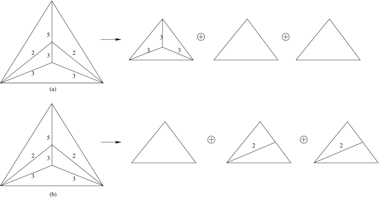
Figure 3: Flow of the orbifold $\mathbb{C}^{3}/\mathbb{Z}_{5(1,3)}$ under marginal deformations

For the marginal deformation by the first twisted sector, eq. (63) gives the flow pattern

$$\mathbb{C}^{3}/\mathbb{Z}_{5(1,3)}\to~{}~{}{\mbox{flat space}}~{}~{}\oplus~{}~{}{\mbox{flat space}}~{}\oplus\mathbb{C}^{3}/\mathbb{Z}_{3(1,1)}$$ (64)

This is shown in fig. (3)(a), where we have split the original triangle along the first twisted sector. Similarly, for deforming the theory by the second twisted sector, we need to consider the $U(1)$ GLSM with four chiral fields of charges $\left(-5,2,2,1\right)$ and in this case the flow is given by

$$\mathbb{C}^{3}/\mathbb{Z}_{5(1,3)}\to~{}~{}{\mbox{flat space}}~{}~{}\oplus~{}~{}\mathbb{C}^{3}/\mathbb{Z}_{2(1,0)}\oplus\mathbb{C}^{3}/\mathbb{Z}_{2(0,1)}$$ (65)

which is given by the diagram in fig. (3)(b). Interestingly, the strength of the continued fractions are not modified in this example. This shows that the decay of supersymmetric $\mathbb{C}^{3}$ orbifolds can be studied from non-supersymmetric $\mathbb{C}^{2}$ orbifolds.

The example we just worked out was an orbifold of the form $\mathbb{C}^{3}/\mathbb{Z}_{n(p,p)}$. It turns out that orbifolds of the form $\mathbb{C}^{3}/\mathbb{Z}_{n(p_{1},p_{2})}$ with $p_{1}$ and $p_{2}$ distinct have a different description, and our method is not very robust in this case. In fact, while the former type of orbifolds do not contain topologically distinct phases, the latter type does. For example, the orbifold $\mathbb{C}^{3}/\mathbb{Z}_{11(2,8)}$ contains topologically distinct phases related by flop transitions [27], corresponding to distinct ways of triangulating the toric diagram for the resolution of this orbifold. This is reflected in the fact that in this case, a combination of the $\mathbb{C}^{2}$ orbifolds does not provide an unique triangulation of the toric diagram. This is evident from fig. (4). The dotted lines indicate in this example the extra lines that we need in order to triangulate the diagram completely (which has $11$ triangles of area $1$), and the solid lines are the Hirzebruch-Jung lines, i.e correspond to the continued fractions that appear in the $\mathbb{C}^{2}$ orbifolds.

Figure 4: Champions meet for the orbifold $\mathbb{C}^{3}/\mathbb{Z}_{11(2,8)}$ marked in solid lines. The strengths of the Hirzebruch-Jung continued fractions for the three $\mathbb{C}^{2}$ orbifolds are marked with each solid line, which we call the Hirzebruch-Jung lines.

Now let us study flow patterns in this supersymmetric example. Consider first turning on the marginal deformation corresponding to the first twisted sector of the theory. This is the point $a$ in fig. (4), with R-charges $\left(\frac{1}{11},\frac{2}{11},\frac{8}{11}\right)$. From Vafa’s construction, this will lead to the decay

$$\mathbb{C}^{3}/\mathbb{Z}_{11(2,8)}\to~{}{\mbox{flat space}}\oplus\mathbb{C}^{3}/\mathbb{Z}_{2(1,0)}\oplus\mathbb{C}^{3}/\mathbb{Z}_{8(2,5)}$$ (66)

This is seen from fig. (4), with the Hirzebruch-Jung integers that have been depicted. Similarly, we can study the decay of this orbifold by turning on a marginal deformation corresponding to the third twisted sector of the theory, with R-charges $\left(\frac{3}{11},\frac{6}{11},\frac{2}{11}\right)$ which is point $b$ in fig. (4). Here, the decay products are three orbifolds of $\mathbb{C}^{3}$ with the quotienting groups being $\mathbb{Z}_{2},\mathbb{Z}_{3},\mathbb{Z}_{6}$, and this decay also can be observed from the figure, as before. However, the decay of this orbifold by turning on a marginal deformation corresponding to the second twisted sector (point $c$ in fig. (4)) is difficult to analyse. This case is complicated because it depends on the phase of the theory being looked at, and the flow cannot be seen as easily as in the previous examples. In particular, we observe that it is difficult to analyse flows that involve triangles which have as one or more edges a line that is not a Hirzebruch-Jung line of any of the $\mathbb{C}^{2}$ orbifolds. This case needs to be studied further.

Finally, let us consider the flows of non-supersymmetric orbifolds of $\mathbb{C}^{3}$, which has been dealt with recently in [6]. In this case, there is no analogue of the construction of [11] as in supersymmetric examples. The latter was a mathematical construction dependent on the fact that the orbifold quotienting group is a finite subgroup of $SL(3,\mathbb{C})$, and those methods cannot be applied for non-supersymmetric $\mathbb{C}^{3}$ orbifolds. However, since we have translated the results to the language of chiral rings earlier in this section, let us try to cast the problem in terms of the generators of the chiral rings. We would like to emphasise that this is just a book-keeping technique for these examples, and does not lead to any mathematical construction analogous to [11].

Again there are two distinct cases to consider here. We will consider one example each of orbifolds of the form $\mathbb{C}^{3}/\mathbb{Z}_{n(p_{1},p_{2})}$, with $p_{1}=p_{2}$ and $p_{1}\neq p_{2}$. Let us first consider type 0 string theory on $\mathbb{C}^{3}/\mathbb{Z}_{13(5,5)}$. From the discussion of the previous subsection, we can construct the chiral ring of this orbifold (the generators of the ring are three elements of R-charges $\left(\frac{1}{13},\frac{5}{13}\frac{5}{13}\right),\left(\frac{3}{13},\frac{2}{13}\frac{2}{13}\right),\left(\frac{8}{13},\frac{1}{13}\frac{1}{13}\right)$) by using the chiral ring generators of the orbifolds $\mathbb{C}^{2}/\mathbb{Z}_{13(5)}$, $\mathbb{C}^{2}/\mathbb{Z}_{13(1)}$ and $\mathbb{C}^{2}/\mathbb{Z}_{13(8)}$. These are the tachyonic (and possibly irrelevant) operators of the world sheet CFT. Further, since we can evaluate the Hirzebruch-Jung integers for these three $\mathbb{C}^{2}$ orbifolds, we can draw a diagram analogous to the supersymmetric examples, with the elements of the chiral ring and the corresponding Hirzebruch-Jung integers. This is shown in fig. (5).

Figure 5: An analogue of the champions meet for the orbifold $\mathbb{C}^{3}/\mathbb{Z}_{13(5,5)}$. The Hirzebruch-Jung integers label each line.

Let us now consider the decay of this orbifold by the relevant operator corresponding to the first twisted sector of this orbifold, which is point $a$ in fig. (5). By our previous analysis, this would correspond to the flow

$$\mathbb{C}^{3}/\mathbb{Z}_{13(5,5)}\to{\mbox{flat space}}\oplus\mathbb{C}^{3}/\mathbb{Z}_{5(2,0)}\oplus\mathbb{C}^{3}/\mathbb{Z}_{5(2,0)}$$ (67)

This flow can be seen from fig. (5), by considering the Hirzebruch-Jung numbers of the corresponding $\mathbb{C}^{2}$ orbifolds. Similarly, the decay of this orbifold by the tachyon of point $b$ (which appears in the third twisted sector) leads to the flow into three $\mathbb{C}^{3}$ orbifolds with the ranks of the orbifolding group being $\mathbb{Z}_{3},\mathbb{Z}_{2},\mathbb{Z}_{2}$, and this can also be seen from the Hirzebruch-Jung numbers of fig. (5). However, we need to be careful here. The Hirzebruch-Jung number of the line that is split in the process of the decay (in this case the line with strength $13$) should be ignored while calculating the action of the orbifolds in the decay process, and the action of the resulting orbifolds should be fixed by the remaining lines. It is not difficult to convince oneself that this uniquely fixes the orbifold action (we will make this clearer in the next example).

Finally, let us consider the type 0 orbifold $\mathbb{C}^{3}/\mathbb{Z}_{13(2,5)}$ which has been studied in details in [6]. The Hirzebruch-Jung continued fraction gives the four generators of the chiral ring in this example, and they are as shown in fig. (6).

Figure 6: An analogue of the champions meet for the orbifold $\mathbb{C}^{3}/\mathbb{Z}_{13(2,5)}$. The interior points are the generators of the chiral ring.

Consider now the condensation of the tachyon corresponding to the first twisted sector (point $a$ in fig. (6), and called $T_{1}$ in [6]). From the figure, we see that this give three $\mathbb{C}^{3}$ spaces, one of which is flat space, one is the terminal singularity $\mathbb{C}^{3}/\mathbb{Z}_{2(1,1)}$ and the third is the supersymmetric orbifold $\mathbb{C}^{3}/\mathbb{Z}_{5(2,2)}$. This also follows from eq. (63).

The tachyon of point $b$ in fig. (6) comes from the third twisted sector of the theory. Thus, in order to study its condensation, we need to consider the corresponding GLSM of four fields with charges $\left(-13,3,6,2\right)$. It is clear that the condensation of this tachyon leads to three $\mathbb{C}^{3}$ orbifolds with quotienting groups $\mathbb{Z}_{3},\mathbb{Z}_{6}$ and $\mathbb{Z}_{2}$. This can also be seen from figure (6) by considering the Hirzebruch-Jung numbers. The details of the orbifold action can be worked out and the results match with [6]. Condensation of the tachyon of the eighth twisted sector (marked point c) is however difficult to follow using our method.

6 Conclusions

In this paper, we have studied in details certain issues regarding localized tachyon condensation on orbifolds of $\mathbb{C}^{2}$ and $\mathbb{C}^{3}$. We have used the GLSM to understand various aspects of the same. We have seen that a computation of the background metric for the GLSM effectively captures much of the physics of closed string tachyon condensation, in lines with [4]. The GLSM also gives a nice way of understanding the number of Coulomb branch vacua of non-supersymmetric backgrounds. Further, we have shown that the decay of $\mathbb{C}^{3}$ orbifolds can be studied in terms of orbifolds of $\mathbb{C}^{2}$.

There are various issues still to be studied. We have mostly considered flows in type 0 string theory, and there are several subtleties that might arise for type II strings, for eg., some of the generators of the chiral ring may be projected out for these [7], and hence the resolution of the singularity cannot be described entirely by Kähler deformations, as we have mentioned before. It will be interesting to understand the interpretation of our results of section 5 in this case.

Secondly, our analysis shows that it is possible to study localized closed string tachyon condensation on orbifolds of the form $\mathbb{C}^{3}/\mathbb{Z}_{n(p_{1},p_{2})}$ starting from two-fold orbifolds of the form $\mathbb{C}^{2}/\mathbb{Z}_{n(k)}$. A better understanding of this is can probably be obtained from the point of view of the GLSM. Specifically, one can ask if the moduli space of GLSMs corresponding to orbifolds of $\mathbb{C}^{3}$ contain, in certain (probably unphysical) limits the orbifolds of $\mathbb{C}^{2}$. We have already seen indications of this in section 5. It would be interesting to explore this issue further.

Conversely, we have also seen that toric geometry of $\mathbb{C}^{3}$ orbifolds contains information about orbifolds of $\mathbb{C}^{2}$, and in most cases there are additional points that need to be removed from the former in order to obtain the latter. It might be possible to study this further from the inverse toric algorithm proposed in [28]. Also, as shown in [10], D-brane gauge theories on orbifolds of the form $\mathbb{C}^{2}/\mathbb{Z}_{n(k)}$ appear to contain various “phases.” However, since the brane probe analysis presented there was valid in the substringy regime, no statement could be made about any duality between these phases, and it was essentially a classical statement about the moduli space of D-brane world volume gauge theories. It might be possible to study such phases by supersymmetric completion of non-supersymmetric two-fold orbifolds to supersymmetric three-folds.

Finally, the issue of obtaining lower dimensional orbifolds starting from the higher dimensional ones might be studied by the boundary state formalism. This would help in unifying the various issues discussed above.

Acknowledgements

We would like to sincerely thank the High Energy Theory Group of Harvard University for their hospitality during the course of this work. Its a pleasure to thank Justin David, Suresh Govindarajan, Ami Hanany, Dileep Jatkar, Shiraz Minwalla, Koushik Ray, Tadashi Takayanagi and Cumrun Vafa for useful discussions. Thanks are due to Utpal Chattopadhyay for computer related help.

References

- [1] A. Sen, “Non-BPS States and Branes in String Theory,” hep-th/9904207
- [2] K. Bardakci, “Dual Models and Spontaneous Symmetry Breaking,” Nucl. Phys. B 68 (1974) 331, K.Bardakci and M.B.Halpern, “Explicit Spontaneous Breakdown in a Dual Model,” Phys. Rev. D10 (1974) 4230, K.Bardakci and M.B.Halpern, “Explicit Spontaneous Breakdown in a Dual Model II: N Point Functions,” Nucl. Phys. B 96 (1975) 285, K.Bardakci, “Spontaneous Symmetry Breakdown in the Standard Dual String Model,” Nucl. Phys. B 133 (1978) 297.
- [3] A. Adams, J. Polchinski and E. Silverstein, “Don’t panic! Closed String Tachyons in ALE spacetimes”, JHEP 0110 (2001) 029. hep-th/0108075
- [4] C. Vafa, “Mirror Symmetry and Closed String Tachyon Condensation,” hep-th/0111051
- [5] J. Harvey, D. Kutasov, E. Martinec and G. Moore, “Localized tachyons and RG flows,” hep-th/0111154
- [6] D. R. Morrison, K. Narayan, M. R. Plesser, “Localized Tachyons in ,” hep-th/0406039
- [7] E. Martinec, G. Moore, “On Decay of K-theory,” hep-th/0212059
- [8] G. Moore, A. Parnachev, “Localized Tachyons and the Quantum McKay Correspondence,” hep-th/0403016.
- [9] E. Witten, “Phases of N=2 Theories in Two Dimensions,” Nuclear Physics B 403, (1993) 159, hep-th/9301042.
- [10] T. Sarkar, “Brane Probes, Toric Geometry, and Closed String Tachyons,” Nucl. Phys. B 648 497 (2003).
- [11] A. Craw, M. Reid, “How to calculate A-Hilb ,” math.AG/9909085.
- [12] S. Minwalla, T. Takayanagi, “Evolution of D-branes Under Closed String Tachyon Condensation,” JHEP 0309 011, 2003, hep-th/0307248
- [13] M. Douglas and G. Moore, “D-branes, quivers and ALE instantons,”hep-th/9603167
- [14] W. Fulton, “Introduction to Toric Varieties,”, Ann. Math. Studies, 131, Princeton University Press, 1993.
- [15] T. Oda, “Convex Bodies and Algebraic Geometry,” Speringer-Verlag, 1988.
- [16] L. Dixon, D. Friedan, E. Martinec, S. Shenker, “The Conformal Field Theory of Orbifolds,” Nucl. Phys. B 282 (1987) 13.
- [17] S-J Sin, “Localized tachyon mass and a g-theorem analogue,” Nucl. Phys. B 667 310 (2003).
- [18] D. R. Morrison, M. R. Plesser, “Summing the Instantons: Quantum Cohomology and Mirror Symmetry in Toric Varieties,” Nucl. Phys. B 440 279, 1995, hep-th/9412236
- [19] P. Aspinwall, “Resolution of Orbifold Singularities in String Theory,” In B. Greene, S. T. Yau (eds)Mirror symmetry II, 355-379, hep-th/9403123i.
- [20] M. Douglas, B. Greene, D. Morrison, “Orbifold Resolution by D-branes,” Nucl. Phys. B 506 84 (1997) hep-th/9704151.
- [21] R. Gregory, J. Harvey, “Spacetime decay of cones at strong coupling,” Class. Quant. Grav. 20 L231, 2003.
- [22] M. Headrick, “Decay of : exact supergravity solutions,” JHEP 0403 025 2004, hep-th/0312213.
- [23] A. Dabholkar, “Tachyon Condensation and Black Hole Entropy,” Phys. Rev. Lett. 88 091301 (2002), hep-th/0111004.
- [24] Y. Okawa, B. Zwiebach, “Twisted Tachyon Condensation in Closed String Field Theory,” JHEP 0403 056 (2004), hep-th/0403051.
- [25] A. Dabholkar, C. Vafa, “tt* Geometry and Closed String Tachyon Potential,” JHEP 0202 008 (2002), hep-th/0111155.
- [26] B. Feng, S. Franco, A. Hanany, Y. H He, “Symmetries of Toric Duality,” JHEP 0212, 076 (2002).
- [27] T. Muto, “D-branes on Orbifolds and Topology Change,” Nucl. Phys B 521, 183 (1998).
- [28] B. Feng, A. Hanany, Y. H He, “D-Brane Gauge Theories from Toric Singularities and Toric Duality,” Nucl.Phys. B 595 165 (2001).