Quantum mechanics in a cut Fock space

Abstract

A recently introduced numerical approach to quantum systems is analyzed. The basis of a Fock space is restricted and represented in an algebraic program. Convergence with increasing size of basis is proved and the difference between discrete and continuous spectrum is stressed. In particular a new scaling low for nonlocalized states is obtained. Exact solutions for several cases as well as general properties of the method are given.

1 Introduction

Recently an attractive possibility of modelling M-theory through relatively simple quantum mechanical systems [1] has occurred. They emerge from the dimensional reduction of supersymmetric gauge theories and provide a simple laboratory to study many properties of supersymmetry [2,3] . It follows from [1] that there is an strong connection between M-theory and $SU(N_{c}\longrightarrow\infty)$ supersymetric Yang-Mills quantum mechanics (SYMQM). However supersymmetric quantum mechanics have much longer history. Various schemes have been analyzed to try to solve the hierarchy problem including the idea of breaking SUSY. This was the reason why SUSY was first studied in the simplest case of quantum mechanics (SUSYQM)[2]. Apart from its physical meaning SUSYQM gave also a deeper understanding of why certain potentials are analytically solvable and other are not [4]. The SYMQM gauge systems were studied for the first time in [3] where the exact spectrum including the ground state of SYMQM D=2 was given. Later on the extension for arbitrary SU(N) gauge group was also obtained [5]. SUSYQM is known to have continuous spectrum due to the fermion-boson cancellation [6]. According to BFSS hypothesis there should be a bound state at the threshold of the spectrum. However, since there are no exact solutions one is forced to use numerical methods.

In this paper we discuss in details a numerical approach of solving quantum mechanical systems proposed in [7,8] and already investigated in [9-13]. Next section contains formulation of the method as well as its general properties. We introduce a cutoff, N, and by means of an algebraic program analyze a complete dependence of the spectrum on the cutoff. We prove that the eigenvalues converge towards exact (i.e in the infinite Hilbert space) spectrum. In section 3 we give the exact spectrum of the momentum and coordinate operators at arbitrary finite $N$. The asymptotic behavior with $N\longrightarrow\infty$ is derived in section 4 where a new scaling law, required to recover the infinite Hilbert space limit, is formulated. The scaling and its universality is discussed in section 5 by giving the exact spectrum of a free particle in quantum mechanics. Interestingly, this solution differs only a little in comparison with the eigenvalues of the hamiltonian for $D=2$ supersymmetric Yang-Mills quantum mechanics at finite cutoff [14]. We prove that the continuum spectrum in quantum mechanics gives rise to the power-like dependance on the cutoff. This result is important in studying supersymmetric systems where the distinction between continuum and discrete spectra is an important issue. In section 6 we use numerical data in order to verify the theoretical results. The implementation of the approach in Mathematica code will be discussed there in details.

2 A cut Fock space

Every quantum hamiltonian can be represented in the eigenbasis of a harmonic oscillator

$$\{\mid n\rangle=\frac{a^{\dagger n}}{\sqrt{n!}}\mid 0\rangle,n\in N\},$$ (1)

where $a,a^{\dagger}$ are the normalized annihilation and creation operators respectively. The correspondence between $a,a^{\dagger}$ and Q, P (coordinate and momentum operators respectively) reads

$$Q=\frac{1}{\sqrt{2}}(a+a^{\dagger}),P=\frac{1}{\sqrt{2i}}(a-a^{\dagger}).$$ (2)

Since this basis is countable it is very convenient to use it in numerical applications. One can limit (1), e.g. $n\leqslant N$, then calculate the finite matrix representation of any hamiltonian and numerically diagonalize above finite matrix to obtain complete spectrum and the eigenstates of the system . The procedure is simple and essentially numerical, however a number of theoretical questions arises while analyzing it. They will be discussed in this paper.

We denote
$H^{(N)}=[H]_{i,j}=h_{i,j}\ \ i,j=1,\ldots,N+1$ as operator $H$ in a cut Fock space (cutoff=N) ,
$E^{(N)}_{m}$ and ${c^{(N)}}_{m}=[{{c^{(N)}}}]^{j}_{m}$  where   $j=1,\ldots,N+1$, $m=1,2,\ldots,N+1$ as eigenvalues and eigenvectors of $H^{(N)}$ respectively, $E_{m}$ and $c_{m}=[c_{m}]^{j}$   as eigenvalues and eigevectors of $H$ respectively. In other words

$$H^{(N)}{c^{(N)}}_{m}=E^{(N)}_{m}c^{(N)}_{m}\ \ \hbox{and}\ \ Hc_{m}=E_{m}c_{m}.$$ (3)

The main aim of present work is to understand the dependence of the spectrum of $H^{(N)}$ on $N$.

3 The spectrum of cut momentum and coordinate operators

Matrix elements of the $P$ and $Q$ operators in the occupation number basis read

$$\langle n\mid Q\mid k\rangle=\sqrt{\frac{k}{2}}\delta_{n,k-1}+\sqrt{\frac{k+1}{2}}\delta_{n,k+1}\ \ ,\ \ \langle n\mid P\mid k\rangle=\frac{1}{i}\sqrt{\frac{k}{2}}\delta_{n,k-1}+\frac{1}{i}\sqrt{\frac{k+1}{2}}\delta_{n,k+1}.$$ (4)

In the Hilbert space limited to maximum of $N$ quanta the eigenvalues of, e.g., momentum are given by zeros of the determinant

$$I_{N+1}=\left|\begin{array}[]{cccccc}-\eta&\sqrt{1}&0&.&.&.\\ -\sqrt{1}&-\eta&\sqrt{2}&.&.&.\\ 0&-\sqrt{2}&-\eta&.&.&.\\ .&.&.&.&.&.\\ .&.&.&.&-\eta&\sqrt{N}\\ .&.&.&.&-\sqrt{N}&-\eta\par\end{array}\right|,\hbox{where}\ \ \eta=i\sqrt{2}\lambda.$$ (5)

Determinant (5) is evaluated by solving recursion relation following from the Laplace expansion. Making a change of variables $J_{N}=\frac{1}{N!}I_{N}$ we obtain

$$(N+2)J_{N+2}+\eta J_{N+1}-J_{N}=0,\ \ J_{1}=-\eta,\ \ J_{2}=\frac{1}{2}({\eta}^{2}+1).$$ (6)

This recursion may be solved using the generating function method. Let us define series with coefficients $J_{N}$

$$F(x)=J_{1}x+J_{2}x^{2}+J_{3}x^{3}+J_{4}x^{4}+\ldots=\sum_{N=1}^{\infty}J_{N}x^{N}.$$ (7)

It follows from (6) that $F(x)$ satisfies

$$(-x+\eta)(F(x)+1)=-F^{\prime}(x),$$ (8)

with the boundary condition $F(0)=0$. The solution reads

$$F(x)=exp\left(\frac{x^{2}}{2}-x\eta\right)-1=\sum_{N=1}^{\infty}\frac{H_{N}(i\frac{\eta}{\sqrt{2}})}{N!}\left(i\frac{x}{\sqrt{2}}\right)^{N},$$ (9)

where $H_{N}(x)$ stands for N-th Hermite polynomial. Since $F(x)$ is analytic at $x=0$, the expansion (9) is unambiguous so $J_{N}=2^{-\frac{N}{2}}i^{N}\frac{H_{N}(i\frac{\eta}{\sqrt{2}})}{N!}$. Then

$$I_{N}=(-1)^{N}2^{-\frac{N}{2}}i^{N}H_{N}(\lambda).$$ (10)

It is clear now that the spectrum of operator $P$ in a cut Fock space is given exactly by zeros of Hermite polynomials. Therefore, denoting $p_{m}^{N}$ as the m-th eigenvalue of cut momentum $P^{(N)}$, we get

$$p^{N}_{m}=z^{(N+1)}_{m},\ \ \ \ \hbox{where}\ \ \ \ H_{N+1}(z^{(N+1)}_{m})=0,\ \ \ \ m=1,2,\ldots,N+1.$$ (11)

This result will be used several times below.

Calculation for coordinate operator $Q$ is very similar. Recursion relation is slightly different but initial conditions also change. Those two differences cancel each other and finally we obtain the same result as for $P$. Therefore, denoting $q_{m}^{N}$ as the m-th eigenvalue of cut coordinate $Q^{(N)}$, we obtain

$$q^{N}_{m}=z^{(N+1)}_{m},\ \ \ \ \hbox{where}\ \ \ \ H_{N+1}(z^{(N+1)}_{m})=0,\ \ \ \ m=1,2,\ldots,N+1.$$ (12)

Since roots of Hermite polynomials are symmetric around $0$, we consider only positive ones for which we introduce the following enumeration

$$0=p^{N}_{0}<p^{N}_{1}<p^{N}_{2}\ldots<p^{N}_{m}<\ldots<p^{N}_{\frac{N}{2}}\ \ \hbox{, \ N - even},$$ (13)

$$p^{N}_{1}<p^{N}_{2}\ldots<p^{N}_{m}<\ldots<p^{N}_{\frac{N+1}{2}}\ \ \hbox{, \ N - odd.}$$ (14)

4 The continuum limit – scaling

Because of the continuum limit it is particularly interesting to analyze the behavior of roots of Hermite polynomials when $N\to\infty$. It is possible to obtain the asymptotic relation ( details are in appendix B )

$$p_{m}^{N}=\frac{\pi m}{\sqrt{2N+3}}\sqrt{1+\frac{{{\pi}^{2}}m^{2}-\frac{3}{2}}{3(2N+3)^{2}}}+O(N^{-4.5}),\ \ m=1,2\ldots,\ldots,\frac{N}{2}\ \ \hbox{N - even},$$ (15)

$$p_{m}^{N}=\frac{\pi(m-\frac{1}{2})}{\sqrt{2N+3}}\sqrt{1+\frac{{{\pi}^{2}}(m-\frac{1}{2})^{2}-\frac{3}{2}}{3(2N+3)^{2}}}+O(N^{-4.5}),\ \ m=1,2\ldots,\ldots,\frac{N+1}{2}\ \ \hbox{N - odd}.$$ (16)

If one naively evaluates the limit $N\to\infty$ for fixed $m$ one obtains $\underbrace{lim_{N\to\infty}}_{m\ fixed}p_{m}^{N}=0$. This is unacceptable, because we know that $\underbrace{lim_{N\to\infty}}_{continuum}p_{m}^{N}=p$ with $p\neq 0$ and $p\neq\infty$. It is clear now that $m$ has to depend on $N$ as follows

$$m=\frac{\sqrt{2N}}{\pi}p+b.$$ (17)

A prescription, that guarantees existence of the continuum limit

$$\lim_{N\longrightarrow\infty}p_{m(N)}^{N}=const.,$$ (18)

is called scaling. The dependence (17) is universal, that is for a large class of observables one obtains nontrivial values when $N\to\infty$. Substituting (17) to (16) and ordering resulting expression with respect to powers of $N$ we get

$$p_{m}^{N}=p+\frac{(b-\frac{1}{2})\pi}{\sqrt{2}}\frac{1}{\sqrt{N}}+\frac{1}{12}p(p^{2}-3)\frac{1}{N}+\frac{\pi}{4\sqrt{2}}(b-\frac{1}{2})(p^{2}-1)\frac{1}{N^{\frac{3}{2}}}+\ldots\ \ .$$ (19)

Notice that $b$ has no influence on the result obtained in the continuum limit. Nevertheless, it is clear that taking $b=\frac{1}{2}$ gives the best convergence.

Moreover one can put

$$m=\frac{\sqrt{2}}{\pi}p\sqrt{N}+b+\frac{c}{\sqrt{N}},$$ (20)

providing another parameter that controls the convergence. Now equation (19) is modified to

$$p_{m}^{N}=p+\frac{(b-\frac{1}{2})\pi}{\sqrt{2}}\frac{1}{\sqrt{N}}+\left(\frac{c\pi}{\sqrt{2}}+\frac{1}{12}p(p^{2}-3)\right)\frac{1}{N}+\frac{\pi}{4\sqrt{2}}(b-\frac{1}{2})(p^{2}-1)\frac{1}{N^{\frac{3}{2}}}+\ldots\ \ .$$ (21)

The procedure may by continued but the optimal values of the coefficients $b,c$ are not universal, i.e. if we take another observable they will be different. We can see this already in the example (19) where coefficient $b$ depends on parity of $N$. Nevertheless the limit (18) is valid for different observables.

It is interesting to deal with the problem of cardinality of the spectrum of the momentum operator. For all $N$ the spectrum of cut operators consists of finite number of eigenvalues but we know that in the continuum limit there has to be an uncountable set of eigenvalues. How those two facts can be brought together? According to (15,16), for large N, there are $N$ eigenvalues ($\frac{N}{2}$ positive ones and $\frac{N}{2}$ negative ones, or $\frac{N-1}{2}$ positive ones and $\frac{N-1}{2}$ negative ones for $N$ even or odd respectively) separated by the distance $O(\frac{1}{\sqrt{N}})$. It means that the spectrum becomes denser so that it is possible to chose such $m(N)$ that

$$\forall_{p\in R}:lim_{N\to\infty}p_{m(N)}^{N}=p.$$ (22)

Therefore the set of all roots of all Hermite polynomials $\mathcal{Z}=\bigcup_{N=1}^{\infty}spectrum(\hat{P}^{(N)})$ is dense in $\mathbb{R}$. However it is not equal to $\mathbb{R}$ because $\mathcal{Z}$ is countable due to the fact that there is countable amount of Hermite polynomials. In other words elements of $\mathcal{Z}$ behave similarly to rational numbers in $\mathbb{R}$. It looks as if there was something wrong because the spectrum of operator $P$ should be continuous. In order to solve this paradox we use the scaling (17). Now any real number $p$ can be obtained in the continuum limit so that all elements of $\mathbb{R}$ are reproduced.

5 The spectrum of the cut kinetic energy

In order to calculate the eigenvalues of a free particle we introduce the cut parity operator

$${\Sigma}^{(N)}=\underbrace{\left[\begin{array}[]{ccccccc}1&0&&0\\ 0&-1&&\\ &&\ddots&\\ 0&&&(-1)^{N}\end{array}\right]}_{N+1\ \ \hbox{columns}}.$$ (23)

A straightforward calculation shows that $[(p^{2})^{(N)},{\Sigma}^{(N)}]=[(p^{(N)})^{2},{\Sigma}^{(N)}]=0$ so that $(p^{2})^{(N)}$ as well as $(p^{(N)})^{2}$, represented in an eigenbasis of ${\Sigma}^{(N)}$, splits into two blocks.

Let $N$ be an odd number. In this case the matrices $(p^{2})^{(N)}$ and $(p^{(N)})^{2}$ contain two blocks ${\frac{N+1}{2}}\times{\frac{N+1}{2}}$ each. We have

$$H^{(N)}=(\frac{1}{2}{p^{2}})^{(N)}=\left[\begin{array}[]{cccccc}&A^{\frac{N+1}{2}}_{+}&&\vrule\lx@intercol\hfil\hfil\lx@intercol&0&\\ \cline{1-6}\cr&0&&\vrule\lx@intercol\hfil\hfil\lx@intercol&A^{\frac{N+1}{2}}_{-}&\\ \end{array}\right],\frac{1}{2}(p^{(N)})^{2}=\left[\begin{array}[]{cccccc}&B^{\frac{N+1}{2}}_{+}&&\vrule\lx@intercol\hfil\hfil\lx@intercol&0&\\ \cline{1-6}\cr&0&&\vrule\lx@intercol\hfil\hfil\lx@intercol&B^{\frac{N+1}{2}}_{-}&\\ \end{array}\right],$$ (24)

where

$$A^{(M)}_{+}=\left[\begin{array}[]{ccccccc}\frac{1}{4}&-\frac{\sqrt{1\cdot 2}}{4}&&0\\ -\frac{\sqrt{1\cdot 2}}{4}&\frac{5}{4}&\ddots&\\ &\ddots&\frac{4M-7}{4}&-\frac{\sqrt{(2M-3)\cdot(2M-2)}}{4}\\ 0&&-\frac{\sqrt{(2M-3)\cdot(2M-2)}}{4}&\frac{4M-3}{4}\end{array}\right],$$ (25)

$$A^{(M)}_{-}=\left[\begin{array}[]{ccccccc}\frac{3}{4}&-\frac{\sqrt{2\cdot 3}}{4}&&0\\ -\frac{\sqrt{2\cdot 3}}{4}&\frac{7}{4}&\ddots&\\ &\ddots&\frac{4M-5}{4}&-\frac{\sqrt{(2M-2)\cdot(2M-1)}}{4}\\ 0&&-\frac{\sqrt{(2M-2)\cdot(2M-1)}}{4}&\frac{4M-1}{4}\end{array}\right],$$ (26)

and

$$B^{(M)}_{+}=\left[\begin{array}[]{ccccccc}\frac{1}{4}&-\frac{\sqrt{1\cdot 2}}{4}&&0\\ -\frac{\sqrt{1\cdot 2}}{4}&\frac{5}{4}&\ddots&\\ &\ddots&\frac{4M-7}{4}&-\frac{\sqrt{(2M-3)\cdot(2M-2)}}{4}\\ 0&&-\frac{\sqrt{(2M-3)\cdot(2M-2)}}{4}&\frac{4M-3}{4}\end{array}\right],$$ (27)

$$B^{(M)}_{-}=\left[\begin{array}[]{ccccccc}\frac{3}{4}&-\frac{\sqrt{2\cdot 3}}{4}&&0\\ -\frac{\sqrt{2\cdot 3}}{4}&\frac{7}{4}&\ddots&\\ &\ddots&\frac{4M-5}{4}&-\frac{\sqrt{(2M-2)\cdot(2M-1)}}{4}\\ 0&&-\frac{\sqrt{(2M-2)\cdot(2M-1)}}{4}&\frac{4M-1}{4}-\frac{2M}{4}\end{array}\right].$$ (28)

Since $A^{(M)}_{+}=B^{(M)}_{+}$ (the + sign corresponds to odd m) therefore

$$E^{N}_{m}\equiv(\frac{1}{2}p^{2})^{N}_{m}=\frac{1}{2}(p^{N}_{m})^{2}\ \ \hbox{ where}\ \ m=1,3,\ldots,N\ \ \hbox{for}\ \ N\ \ -\ \ \hbox{odd}.$$ (29)

When $N$ is even, the analogous procedure gives

$$E^{N}_{m}\equiv(\frac{1}{2}p^{2})^{N}_{m}=\frac{1}{2}(p^{N}_{m})^{2}\ \ \hbox{ where}\ \ m=2,4,\ldots,N\ \ \hbox{for}\ \ N\ \ -\ \ \hbox{even}.$$ (30)

Now it is useful to present the eigenvalues (29,30) in the following table. For example for $N<4$, $m<5$

$$\left(\begin{array}[]{cccccc}E^{0}_{1}={\large\textbf{?}}&E^{1}_{1}=\frac{1}{2}(p^{1}_{1})^{2}&E^{2}_{1}={\large\textbf{?}}&E^{3}_{1}=\frac{1}{2}(p^{3}_{1})^{2}\\ &&&\\ -&E^{1}_{2}={\large\textbf{?}}&E^{2}_{2}=\frac{1}{2}(p^{2}_{2})^{2}&E^{3}_{2}={\large\textbf{?}}\\ &&&\\ -&-&E^{2}_{3}={\large\textbf{?}}&E^{3}_{3}=\frac{1}{2}(p^{3}_{3})^{2}\\ &&&\\ -&-&-&E^{3}_{4}={\large\textbf{?}}\\ &&&\\ \end{array}\right).$$ (31)

We prove that fields filled with questionmarks in (31) are equal to their neighbors on the right.

Let $N$ be an odd number. We have already shown that matrix $(\frac{1}{2}p^{2})^{(N)}$ contains two blocks (24). Now, if we increase $N\longrightarrow N+1$ we obtain

$$(\frac{1}{2}{p^{2}})^{(N+1)}=\left[\begin{array}[]{ccccccc}&&&\vrule\lx@intercol\hfil\vdots\hfil\lx@intercol&\vrule\lx@intercol\hfil\hfil\lx@intercol&&\\ &A^{\frac{N+1}{2}}_{+}&&\vrule\lx@intercol\hfil 0\hfil\lx@intercol&\vrule\lx@intercol\hfil\hfil\lx@intercol&0&\\ &&&\vrule\lx@intercol\hfil\bullet\hfil\lx@intercol&\vrule\lx@intercol\hfil\hfil\lx@intercol&&\\ \cline{1-3}\cr 0&\ldots\ \ \ 0&\bullet&0&\vrule\lx@intercol\hfil\hfil\lx@intercol&&\\ \cline{1-6}\cr&&&&\vrule\lx@intercol\hfil\hfil\lx@intercol&&\\ &0&&&\vrule\lx@intercol\hfil\hfil\lx@intercol&A^{\frac{N+1}{2}}_{-}&\\ &&&&\vrule\lx@intercol\hfil\hfil\lx@intercol&&\end{array}\right],$$ (32)

so that the block $A^{\frac{N+1}{2}}_{-}$ does not change. It means that in the $N+1$ cutoff, eigenvalues from this block remain untouched. This block corresponds to even $m$, therefore we have

$$E^{(N+1)}_{m}=E^{(N)}_{m}\ \ \hbox{for}\ \ m=2,4,\ldots,N+1\ \ \hbox{ N - odd}.$$ (33)

When $N$ is even an analogous procedure gives

$$E^{(N+1)}_{m}=E^{(N)}_{m}\ \ \hbox{for}\ \ m=1,3,\ldots,N\ \ \hbox{ N - even}.$$ (34)

That completes the whole spectrum of ${(\frac{1}{2}p^{2})}^{(N)}$. First few exemplary values are

$$\left|\begin{array}[]{cccccc}0.25&0.25&0.137&0.137&0.095&0.095\\ -&0.75&0.75&0.459&0.459&0.333\\ -&-&1.362&1.362&0.892&0.892\\ -&-&-&2.040&2.040&1.400\\ -&-&-&-&2.762&2.762\\ -&-&-&-&-&3.516\end{array}\right|.$$

Above numbers were obtained from a program described in next section and indeed confirm (33,34). According to (15,16) formulas (29,30,33,34) give

$$E^{(N)}_{m}\approx\frac{\pi^{2}}{2}\frac{(m-\frac{1}{2})^{2}}{2N+3}\ \ \ \hbox{ N - odd}\ \ \ \hbox{ m - odd },\\$$ (35)

$$E^{(N)}_{m}\approx\frac{\pi^{2}}{2}\frac{m^{2}}{2N+5}\ \ \ \hbox{ N - odd}\ \ \ \hbox{ m - even },\\$$ (36)

$$E^{(N)}_{m}\approx\frac{\pi^{2}}{2}\frac{(m-\frac{1}{2})^{2}}{2N+5}\ \ \ \hbox{ N - even}\ \ \ \hbox{ m - odd },\\$$ (37)

$$E^{(N)}_{m}\approx\frac{\pi^{2}}{2}\frac{m^{2}}{2N+3}\ \ \ \hbox{ N - even}\ \ \ \hbox{ m - even },\\$$ (38)

Note that (17) applied to each (35,36,37,38) separately gives the expected limit $\frac{p^{2}}{2}$. Moreover we see that the dependence of spectrum on $N$ is power like i.e. slow.

6 Applications

In this section we use above analytic results to verify the method introduced in [7,8]. It consists of numerical diagonalization of finite matrices and extrapolation of results to $N\to\infty$. Practically, when one deals with fast convergence of eigenvalues it is sufficient to stop the calculations for relatively low cutoff N ( in the case of one dimensional nonrelativistic quantum mechanics the results for N=50 are already very accurate ). Nevertheless a problem may occur when the convergence is slow ( polynomial ), or when numerical calculations are time consuming even for low N.

One of aims of this work is better understanding the case of a free particle which has the former feature. The later situation occurs everytime when there are higher dimensions. Models discussed in [7,8] have both of those difficulties, therefore it is crucial to understand analytically the asymptotics of the spectrum for large $N$. We expect that the power-like behavior in $N$ is characteristic not only for the spectrum of a free particle but also it occurs in every scattering problem because in those cases the asymptotics of wave functions is the same as for a free particle so that the asymptotic momentum may be properly defined.

6.1 Quantum mechanics on a computer

Let us discuss in details the implementation of the method [7,8] in the computer code. Consider quantum system with $D$ degrees of freedom with $D$ creation and annihilation operators. One can construct the whole orthogonal basis from the vacuum state $\mid 0\rangle$

$$\mid n_{1},n_{2},\ldots,n_{D}\rangle=\frac{(\widehat{a}_{1}^{\dagger})^{n_{1}}}{\sqrt{n_{1}!}}\frac{(\widehat{a}_{2}^{\dagger})^{n_{2}}}{\sqrt{n_{2}!}}\ldots\frac{(\widehat{a}_{D}^{\dagger})^{n_{D}}}{\sqrt{n_{D}!}}\mid 0\rangle.$$ (39)

Each state in a cut Fock space, decomposed in this basis, is represented as a list in Mathematica program

$$\mid\psi\rangle=\sum_{k=1}^{p}a_{k}\mid n_{1}^{k},n_{2}^{k},\ldots,n_{D}^{k}\rangle\longrightarrow$$

$$\Bigl{\{}p,\{a_{1},a_{2},\ldots,a_{p}\},\bigl{\{}\{n_{1}^{1},n_{2}^{1},\ldots,n_{D}^{1}\},\{n_{1}^{2},n_{2}^{2},\ldots,n_{D}^{2}\},\ldots,\{n_{1}^{p},n_{2}^{p},\ldots,n_{D}^{p}\}\bigr{\}}\Bigr{\}}.$$ (40)

The first element of this list specifies the number of basis vectors, that the state $\mid\psi\rangle$ is decomposed on . The second element of the list is a list of coefficients of this decomposition. Basis vectors are represented in the third element of this list. For example

$$a\mid 0,1\rangle+b\mid 1,0\rangle+c\mid 1,1\rangle\longrightarrow\Bigl{\{}3,\{a,b,c\},\bigl{\{}\{0,1\},\{1,0\},\{1,1\}\bigr{\}}\Bigr{\}}.$$

The creation and annihilation operators

$$\widehat{a}_{k}:\ \ \ \widehat{a}_{k}\mid n_{1},n_{2},\ldots,n_{k},\ldots,n_{D}\rangle=\sqrt{n_{k}}\mid n_{1},n_{2},\ldots,n_{k}-1,\ldots,n_{D}\rangle,$$ (41)

$$\widehat{a}_{k}^{\dagger}:\ \ \ \widehat{a}_{k}^{\dagger}\mid n_{1},n_{2},\ldots,n_{k},\ldots,n_{D}\rangle=\sqrt{n_{k}+1}\mid n_{1},n_{2},\ldots,n_{k}+1,\ldots,n_{D}\rangle.$$ (42)

have the following action in the list representation

$$\widehat{a}_{k}\mid\psi\rangle\longrightarrow\Bigl{\{}p,\{\sqrt{n_{k}^{1}}a_{1},\ldots,\sqrt{n_{k}^{p}}a_{n}\},\bigl{\{}\{n_{1}^{1},\ldots,n_{k}^{1}-1,\ldots,n_{D}^{1}\},\{n_{1}^{2},\ldots,n_{k}^{2}-1,\ldots,n_{D}^{2}\},\ldots,$$

$$\ldots,\{n_{1}^{p},\ldots,n_{k}^{p}-1,\ldots,n_{D}^{p}\}\bigr{\}}\Bigr{\}},$$ (43)

and

$$\widehat{a}_{k}^{\dagger}\mid\psi\rangle\longrightarrow\Bigl{\{}p,\{\sqrt{n_{k}^{1}+1}a_{1},\ldots,\sqrt{n_{k}^{p}+1}a_{p}\},\bigl{\{}\{n_{1}^{1},\ldots,n_{k}^{1}+1,\ldots,n_{D}^{1}\},\{n_{1}^{2},\ldots,n_{k}^{2}+1,\ldots,n_{D}^{2}\},\ldots,$$

$$\ldots\{n_{1}^{p},\ldots,n_{k}^{p}+1,\ldots,n_{D}^{p}\}\bigr{\}}\Bigr{\}}.$$ (44)

In order to evaluate the matrix representation of any observble we define procedures which add and multiply on arbitrary state by a complex number as well as scalar multiply states. For example

$$\mid\psi\rangle\longrightarrow\Bigl{\{}2,\{1,2\},\bigl{\{}\{0,0\},\{0,1\}\bigl{\}}\Bigl{\}},$$

$$\mid\phi\rangle\longrightarrow\Bigl{\{}2,\{1,1\},\bigl{\{}\{0,2\},\{0,1\}\bigl{\}}\Bigl{\}},$$

then

$$\mid\psi\rangle+\mid\phi\rangle\longrightarrow\Bigl{\{}3,\{1,3,1\},\bigl{\{}\{0,0\},\{0,1\},\{0,2\}\bigl{\}}\Bigl{\}},$$

$$2\mid\phi\rangle\longrightarrow\Bigl{\{}2,\{2,2\},\bigl{\{}\{0,2\},\{0,1\}\bigl{\}}\Bigl{\}},$$

and

$$\langle\psi\mid\phi\rangle\longrightarrow 2.$$

Adding lists is simply adding those coefficients of the decomposition (40), that have the same basis vectors. If decompositions of $\mid\psi\rangle$ and $\mid\psi\rangle$ have different basis vectors then the sublist consisting of basis vectors has to be extended accordingly.

The procedure of multiplying the state by a number reduces to multiplying the list of coefficients by this number.

Scalar multiplication $\langle\psi\mid\phi\rangle$ reduces to a search for common basis vectors occurring in decomposition of $\mid\psi\rangle$ and $\mid\phi\rangle$. Afterwards proper coefficients and their complex conjugations have to be multiplied.

These rules allow to automatically represent any operator in a cut basis (39).

6.2 Numerical diagonalization

Here we compare numerical data and analytic results of section 3for

a1) eigenvalues of $P^{(N)}$ evaluated by the program described in 6.1. ( according to section 3 they are exactly the roots of Hermite polynomials ),

a2) the asymptotic form (16),

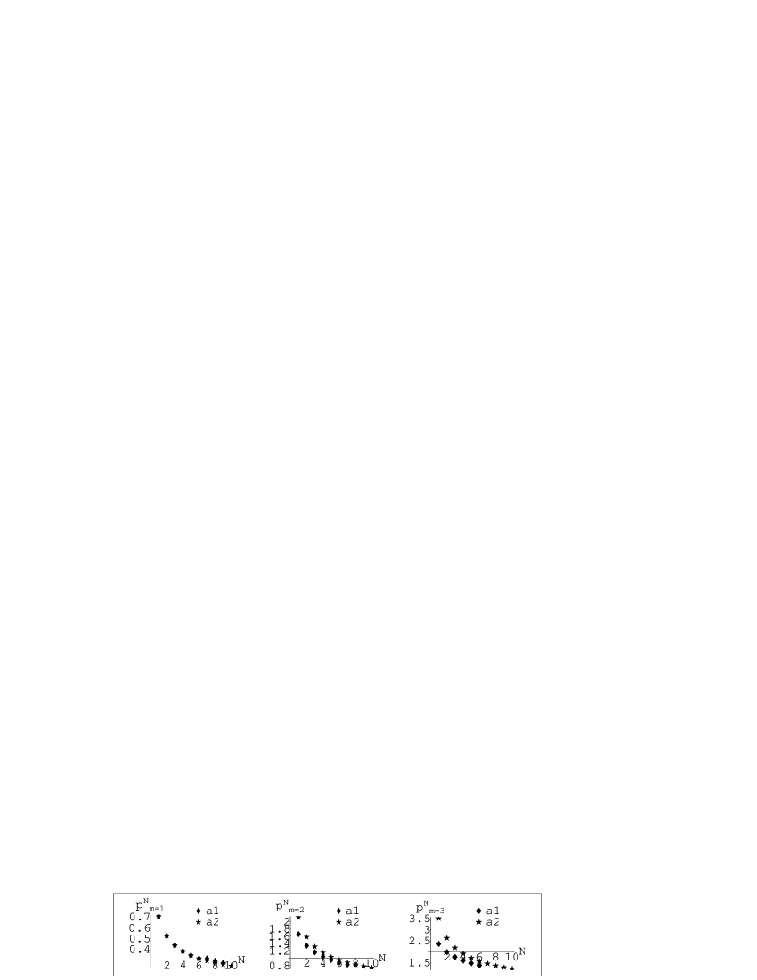
Figure 1: Asymptotic, a2), and exact, a1), behavior of $p^{(N)}_{m}$ for m=1,2,3.

Figure 1 presents the comparison of cases a1 and a2 for m=1,2,3. The approximate value is obtained from (16) by taking only the leading term

$$p^{N}_{m}\approx\frac{\pi(m-\frac{1}{2})}{\sqrt{2N+1}}.$$ (45)

We see that there is a good agreement between exact and approximate values even for low $N$, and it gets worse for higher $m$ where next terms of the expansion of (16) are important.

6.3 Continuum limit on a computer

Here we want to obtain dispersion relation that is the dependence of the energy on momentum $E(p)$. Obviously we know that $E(p)=\frac{p^{2}}{2}$ but it is only because we are able to solve Schrödinger equation for a free particle. However one has to put himself in a situation where there is a certain set of eigenvalues ${E}^{N}_{m}$ and no information about the dispersion relation is available. In other words the question is how to obtain unknown a priori function $E(p)$ by means of eigenvalues ${E}^{N}_{m}$? In order to do this one has to make $m$ dependent on $N$ : $m=m(N,p)$ such that the limit

$$\lim_{N\to\infty}{E}^{N}_{m(N,p)}=E(p),$$ (46)

is not trivial that is $E(p)<\infty$ and $E(p)\neq 0$. Note that (46) automatically requires the set $\{{E}^{N}_{m}:m,N\in\mathbb{N}\}$ to be dense in $E(\mathbb{R})$ . In case of a free particle ($E(\mathbb{R})=[0,\infty)$) we can even construct this set (squares of roots of Hermite polynomials) however it is a general property of any operator with continuous spectrum. This is exactly the reason why ${E}^{N}_{m}$ depend on N as a power rather then exponentially.

Let us emphasize that we don’t have to know the dependence $E(p)$ to evaluate $m(N)$. This is because the relation $m(N)$ was established on grounds of the condition that there has to exist the continuum limit for the momentum, so that any other operator commuting with $P$ will have the same scaling. We will analyze in details the case of a free particle in nonrelativistic quantum mechanics but another example may be Dirac equation where we expect that the scaling law (18) will give $E(p)=\sqrt{M^{2}+p^{2}}$. Therefore the scaling in (46) has to be the same as for momentum operator, that is

$$m(N,p)=\frac{\sqrt{2N}}{\pi}p+\frac{1}{2}.$$ (47)

However in formula (47) we have to introduce a certain change

$$m(N,p)\longrightarrow 2m(N,p)=2\frac{\sqrt{2N}}{\pi}p+1,$$ (48)

because the scaling (48) is meant for positive eigenvalues of operator $P^{(N)}$ only. Let us consider an example of $N=7$. The spectrum of operator $P^{(8)}$ consists of roots of $H_{8}(x)$, so that we have 8 roots where 4 of them are positive and 4 are negative.

Now, if we square them the spectrum becomes positive and the numeration of eigenvalues changes as follows.

For example, the eigenvalue that we used to number as the first one will now have the index $m=2$, the eigenvalue that we used to number as the second one will now have the index $m=4$ ect. Therefore the formula (47) has to be rescaled as in (48).

According to (48), eigenvalues ${E}^{N}_{m}$ are analyzed by fixing any momentum value $p$ and writing down the value ${E}^{N_{max}}_{m(N_{max},p)}$ where $N_{max}$ is the highest N in computer calculations. Then we change the momentum value and repeat the procedure. In this way one obtains an approximate ( because of limited value of $N$ ) dependence $E(p)$, which should reproduce $\frac{p^{2}}{2}$ for a free particle. However the problem concerning the formula $m(N,p)$ occurs because $m$ is not a natural number. We circumvent this by taking an integer part ( INT ) of Eq.(48), so that the matrix index is $INT(m(N_{max},p))$, where $N$ is an even number. The convergence of those elements was checked in Mathematica for $p=1,2,3,\ldots,37$ (e.g. Figure 2)

Figure 2: The convergence of ${{E}}^{N}_{INT(m(N_{max},p))}$ for p=1 and p=10 respectively.

Figure 3: The convergence of ${{E}}^{N}_{INT(m(N_{max},p))}$ for p=1.

This behavior can be understood as follows. If one plots the dependence of ${E}^{N}_{1}$ on N ( p is fixed ), one obtains (35-38) a hyperbola. The lower index $m=1$ specifies the first eigenvalue. The upper index enumerates the cutoff. If we plot the dependence of ${E}^{N}_{2}$ on N, we get another hyperbola ect. Finally the plot of ${E}^{N}_{m}$ is a set of hyperbolas on a plane ( see Figure 3). The scaling that we have used previously means that from each hyperbola we are taking only one point in such way that in the limit of large $N$ a constant value is reproduced. Why on those figures we see cut hyperbolas instead of points? This is because we had to introduce the INT procedure which is equivocal. In a consequence it is possible that for different cutoffs ( say N and N’ ) there is $INT(m(N,p))=INT(m(N^{\prime},p))$. It means that points $(N,INT(m(N,p)))$ and $(N^{\prime},INT(m(N^{\prime},p)))$ are on the same hyperbola. Eventually $N$ will be large enough so that the INT operation notices the difference and the point "jumps" to next hyperbola. Let us also note that the scaling (18) is an asymptotic law hance for low N the behavior of ${E}^{N}_{m(N,p)}$ may vary for different values of p. This effect accounts for the different behavior in Figure 2a and 2b.

The dispersion relation extracted in this way is presented in Figure 4. This result has no error because all eigenvalues are precisely evaluated hance any statistical interpretation is meaningless. The tangent coefficient $0.5365$ is different from $0.5$ but we did expect that because it is a numerical result obtained on grounds of limited cutoff. Moreover we had to introduce the INT operation. In a consequence we had to choose only one point from cut hyperbolas. It is a source of a new error which gets smaller while the cutoff increases.

Therefore Figure 4 confirms that we can obtain the dispersion relation from the knowledge of the spectrum of a cut hamiltonian.

Figure 4: Reproduced dispersion relation.

7 Bound states versus scattering states

In this section we stress the difference between localized and nonlocalized states. It follows from simple algebra ( see Appendix A) that

$$E_{m}-E^{(N)}_{m}=\frac{\sum_{j=1}^{N}\sum_{j=N+1}^{\infty}h_{ij}c^{j}_{m}}{\sum_{i=1}^{N}{c}^{j}_{m}{{c^{*}}^{(N)}}^{j}_{m}},$$ (49)

which means that the spectrum of cut operators converges towards the spectrum of operators in infinite Hilbert space. Moreover one can tell how fast is the convergence because from (49) it is clear that the convergence $E^{(N)}_{m}\xrightarrow[N\longrightarrow\infty]{}E_{m}$ is governed by the behavior of the $c^{j}_{m}$ at large $j$. Note that in (49) $c^{j}_{m}$ are the exact components of eigenvectors of $H$. This is exactly the result we were anticipating because the difference between localized and non-localized states lies in components $c^{j}_{m}$. Therefore one can numerically judge weather the state is bound or not on grounds of the behavior of the eigenvalues of cut operators only.

For the case of a free particle one can obtain $c^{n}_{E}$ exactly

$$c^{n}_{E}=\langle n\mid k\rangle=\int_{R}dx\langle n\mid x\rangle\langle x\mid k\rangle=\int_{R}dx\psi^{H.O.}_{n}(x)e^{ikx},$$ (50)

where H.O. stands for harmonic oscillator

$$\psi^{H.O.}_{n}(x)=\frac{1}{\sqrt{2^{n}n!\pi}}H_{n}(x)e^{-x^{2}/2}.$$ (51)

Integral (50) is evaluated with the aid of some analytic properties of Hermite polynomials, what is presented in Appendix C. The result is

$$c^{n}_{E}=\sqrt{2\pi}i^{n}\psi^{H.O.}_{n}(k).$$ (52)

Figure 5 is an example of (52) for $E=\frac{k^{2}}{2}=1000$.

Figure 5: Components of the eigenvector (E=1000) for free particle.

Asymptotic behavior of the envelope is ( see Appendix C ) $\mid c^{n}_{E}\mid\approx\sqrt[4]{\frac{2}{\pi n}}$ which is indeed power like .

Similar calculations for discrete spectrum are not known, so one is left with numerical data instead. Figure 6 presents components of eigenvector corresponding to the first (the lowest) eigenvalue of anharmonic oscillator, as well as the convergence of the first eigenvalue.

Figure 6: Components of the eigenvector ($c^{j}_{m=1}$) and the the convergence of eigenvalues ($E^{N}_{m=1}$) for anharmonic oscillator.

In this case the behavior of $c^{j}_{m}$ is completely different from one shown in Figure 5. One sees that $E^{N}_{m}$ varies in the same ( exponential ) way as $c^{j}_{m}$. In other words, the behavior of eigenvalues $E^{N}_{m}$ with the cutoff $N$ distinguishes wether the state is bound or not.

8 Conclusions

The main purpose of this paper was to prove that the method proposed in [7,8] enables to distinguish numerically weather the state is localized or not. This aim and related problems have already been investigated [9-13]. This distinction is an important issue while studying supersymmetric models (D=10 SYMQM) where bound states exist among dense number of scattering ones [1]. Therefore one has to reanalyze quantum systems from the very beginning in a new manner. Starting from the calculation of spectrum of cut operators $Q^{(N)},P^{(N)}$one realizes that eigenvalues of those operators are exactly equal to the roots of Hermite polynomials. Next, we conclude that in order to recover the continuum limit one has to introduce scaling $m(N)$. The validity of the scaling law in the hamiltonian of a free particle was rigourously proven in section 5 and numerically tested in section 6. As a result one reproduces the dispersion relation from an information about a spectrum of a cut hamiltonian. It is expected that the same scaling may be applied for a set of hamiltonians commuting with $P$ or under weaker assumptions, namely those for which $P$ can be defined asymptotically. The scaling in higher dimensions is important because of the occurrence of scattering states (e.g SYMQM D=2 systems). The formula (18) is expected to be valid in those cases because they are described by quantum mechanics of a free particle in color dimensions. In this case the coefficient in (17) may be different, however (18) is claimed to be applicable all the time. In particular D=2, SU(2) SYMQM [10] is free and it has been found [14] that the system requires (17) exactly to recover the continuum limit. Recently a new possibility to speed up the numerical approach in D=4 has occurred [11]. The naive diagonalization of the Hamiltonian in the whole cut Hilbert space was abandoned and replaced by the language of rotational invariance. The new approach can be extended to higher dimensions as well.

9 Acknowledgments

I am very grateful to my supervisor Prof. Jacek Wosiek for priceless advices and comments concerning this paper. This work was supported by the Polish Committee for Scientific Research under grants no. PB 2P03B 09622 and no. PB 1P03B 02427.

10 Appendix A

Here we derive the formula (49). Let us start with eigen equation $Hc_{m}=E_{m}c_{m}$ where $H$ is an operator and $c_{m}$ its eigenvector. Writing it in the matrix form

$$\left[\begin{array}[]{ccccccc}&&&\vrule\lx@intercol\hfil h_{1\ N+1}\hfil\lx@intercol&\ldots&\\ &H^{(N)}&&\vrule\lx@intercol\hfil\vdots\hfil\lx@intercol&\cdots&\\ &&&\vrule\lx@intercol\hfil h_{N\ N+1}\hfil\lx@intercol&\ldots&\\ \cline{1-3}\cr h_{N+1\ 1}&\ldots&h_{N+1\ N}&h_{N+1\ N+1}&\ldots&\\ \vdots&\vdots&\vdots&\vdots&\vdots&\end{array}\right]\left[\begin{array}[]{ccccccc}c^{1}_{m}\\ \vdots\\ c^{N}_{m}\\ c^{N+1}_{m}\\ \vdots\\ \end{array}\right]=E_{m}\left[\begin{array}[]{ccccccc}c^{1}_{m}\\ \vdots\\ c^{N}_{m}\\ c^{N+1}_{m}\\ \vdots\\ \end{array}\right],$$ (53)

and rewriting for first N components only one obtains

$$H^{(N)}\left[\begin{array}[]{ccccccc}c^{1}_{m}\\ \vdots\\ c^{N}_{m}\\ \end{array}\right]+\left[\begin{array}[]{ccccccc}\sum_{i=1}^{\infty}h_{1\ N+i}c^{N+i}_{m}\\ \vdots\\ \sum_{i=1}^{\infty}h_{N\ N+i}c^{N+i}_{m}\\ \end{array}\right]=E_{m}\left[\begin{array}[]{ccccccc}c^{1}_{m}\\ \vdots\\ c^{N}_{m}\\ \end{array}\right].$$ (54)

Now complex conjugate (54) and multiply it by ${c^{(N)}}_{n}$ from the right side

$$\left[\begin{array}[]{ccccccc}{c^{*}}^{1}_{m}&\ldots&{c^{*}}^{N}_{m}\end{array}\right]H^{(N)}\left[\begin{array}[]{ccccccc}{c^{(N)}}^{1}_{n}\\ \vdots\\ {c^{(N)}}^{N}_{n}\\ \end{array}\right]+\left[\begin{array}[]{ccccccc}\sum_{i=1}^{\infty}{h^{*}}_{1,N+i}{c^{*}}^{N+i}_{m}&,\ldots,&\sum_{i=1}^{\infty}{h^{*}}_{N,N+i}{c^{*}}^{N+i}_{m}\end{array}\right]\left[\begin{array}[]{ccccccc}{c^{(N)}}^{1}_{n}\\ \vdots\\ {c^{(N)}}^{N}_{n}\\ \end{array}\right]=$$

$$E_{m}\left[\begin{array}[]{ccccccc}{c^{*}}^{1}_{m}&\ldots&{c^{*}}^{N}_{m}\end{array}\right]\left[\begin{array}[]{ccccccc}{c^{(N)}}^{1}_{n}\\ \vdots\\ {c^{(N)}}^{N}_{n}\\ \end{array}\right],$$ (55)

so that

$$E^{(N)}_{m}\sum_{i=1}^{N}{c^{*}}^{j}_{m}{c^{(N)}}^{j}_{n}+\sum_{i=1}^{N}\sum_{j=N+1}^{\infty}{h^{*}}_{ij}{c^{*}}^{j}_{n}=E_{m}\sum_{i=1}^{N}{c^{*}}^{j}_{m}{c^{(N)}}^{j}_{n},$$ (56)

or

$$(E_{m}-E^{(N)}_{n})\sum_{i=1}^{N}{c^{*}}^{j}_{m}{c^{(N)}}^{j}_{n}=\sum_{i=1}^{N}\sum_{j=N+1}^{\infty}{h^{*}}_{ij}{c^{*}}^{j}_{n},$$ (57)

it is non trivial to realize that above equation means that $\sum_{i=1}^{N}{c^{*}}^{j}_{m}{c^{(N)}}^{j}_{n}\longrightarrow\delta_{mn}$ thus one can omit the $n$ index and write

$$E_{m}-E^{(N)}_{m}=\frac{\sum_{i=1}^{N}\sum_{j=N+1}^{\infty}h_{ij}c^{j}_{m}}{\sum_{i=1}^{N}{c}^{j}_{m}{{c^{*}}^{(N)}}^{j}_{m}}.$$ (58)

Of course this derivation is for the case with discrete spectrum (discrete index m ) nevertheless for continuous spectrum the same calculations give

$$(E-E^{(N)}_{n})\sum_{i=1}^{N}{c^{*}}^{j}_{E}{c^{(N)}}^{j}_{n}=\sum_{i=1}^{N}\sum_{j=N+1}^{\infty}{h^{*}}_{ij}{c^{*}}^{j}_{E},$$ (59)

where

$$H^{(N)}{c^{(N)}}_{E}=E^{(N)}_{E}c^{(N)}_{E}\ \ \ \hbox{and}\ \ \ Hc_{E}=Ec_{E}\ \ \ E\in R.$$ (60)

This case is discussed in details in sections 6 and 7.

11 Appendix B

In this appendix we derive the asymptotic form of the zeros $q_{m}^{n}$ of the Hermite polynomial $H_{n}(z)$. When $n$ is an even number they may be obtained using the following relation [14]

$$H_{n}(z)=(-1)^{\frac{n}{2}}2^{n}{\frac{1}{2}n}!L_{{\frac{n}{2}}}^{-\frac{1}{2}}(z^{2}),$$ (61)

where $n$ is an even number, $L_{n}^{\alpha}(z^{2})$ are the generalized Laguerre polynomials with parameter $\alpha$ (in out case $\alpha=-\frac{1}{2}$). Let $z_{m}^{n}$ ,$t_{m,\alpha}^{\frac{n}{2}}$ and $j_{m,\alpha}$ denote the m-th positive root of $H_{n}(z)$, ${L_{\frac{n}{2}}}^{\alpha}(z)$ and $J_{\alpha}(z)$. One has [14]

$$t_{m,\alpha}^{\frac{n}{2}}=\frac{{j_{m,\alpha}}^{2}}{4k_{\frac{n}{2}}}\left(1+\frac{2({\alpha}^{2}-1)+{j_{m,\alpha}}^{2}}{48{k_{\frac{n}{2}}}^{2}}\right)+O(n^{-5}),$$ (62)

where

$$k_{\frac{n}{2},\alpha}=\frac{n}{2}+\frac{\alpha+1}{2}\ \ \hbox{ and }\ \ (z_{m,\alpha}^{n})^{2}=t_{m,\alpha}^{\frac{n}{2}}.$$ (63)

For $\alpha=-\frac{1}{2}$ we obtain $J_{-\frac{1}{2}}(z)=\sqrt{\frac{2}{{\pi}z}}cos(z)$, therefore $j_{\alpha,m}=\pi(m-\frac{1}{2})$ where $m=1,2\ldots,\ldots,\frac{n}{2}$ and $k_{\frac{n}{2},\alpha}=\frac{n}{2}+\frac{1}{4}$ so

$$(z_{m}^{n})^{2}=\frac{{{\pi}^{2}}(m-\frac{1}{2})^{2}}{4(\frac{n}{2}+\frac{1}{4})}\left(1+\frac{{{\pi}^{2}}(m-\frac{1}{2})^{2}-\frac{3}{2}}{48(\frac{n}{2}+\frac{1}{4})^{2}}\right)+O(n^{-5})=$$

$$=\frac{{{\pi}^{2}}(m-\frac{1}{2})^{2}}{2n+1}\left(1+\frac{{{\pi}^{2}}(m-\frac{1}{2})^{2}-\frac{3}{4}}{3(2n+1)^{2}}\right)+O(n^{-5}).$$ (64)

Let us define ( $m$ is fixed )

$$f(n):=\frac{{{\pi}^{2}}(m-\frac{1}{2})^{2}}{2n+1}\left(1+\frac{{{\pi}^{2}}(m-\frac{1}{2})^{2}-\frac{3}{4}}{3(2n+1)^{2}}\right)=\frac{a}{n}+\frac{b}{n^{2}}+\frac{c}{n^{3}}+\ldots\ \ ,$$ (65)

we have

$$z_{m}^{n}=\sqrt{f(n)+O(n^{-5})}=\sqrt{f(n)}\sqrt{1+\frac{O(n^{-5})}{f(n)}}\approx\sqrt{f(n)}(1+\frac{1}{2}O(n^{-4}))=\sqrt{f(n)}(1+O(n^{-4})),$$ (66)

so

$$z_{m}^{n}=\sqrt{f(n)}+\sqrt{f(n)}O(n^{-4})=\sqrt{f(n)}+O(n^{-4.5}),$$ (67)

finally

$$z_{m}^{n}=\frac{\pi(m-\frac{1}{2})}{\sqrt{2n+1}}\sqrt{1+\frac{{{\pi}^{2}}(m-\frac{1}{2})^{2}-\frac{3}{2}}{3(2n+1)^{2}}}+O(n^{-4.5}).$$ (68)

When $n$ is an odd number there are [10] analogous relations

$$H_{n}(z)=(-1)^{\frac{n-1}{2}}2^{n}{(\frac{n-1}{2})}!zL_{{\frac{n-1}{2}}}^{\frac{1}{2}}(z^{2}),$$ (69)

and

$$t_{m,\alpha}^{\frac{n-1}{2}}=\frac{{j_{m,\alpha}}^{2}}{4k_{\frac{n-1}{2}}}\left(1+\frac{2({\alpha}^{2}-1)+{j_{m,\alpha}}^{2}}{48{k_{\frac{n-1}{2}}}^{2}}\right)+O(n^{-5}),\ \$$ (70)

where

$$k_{\frac{n-1}{2},\alpha}=\frac{n-1}{2}+\frac{\alpha+1}{2}\ \ \hbox{ and }\ \ (z_{m,\alpha}^{n-1})^{2}=t_{m,\alpha}^{\frac{n-1}{2}}.$$ (71)

In this case $J_{\alpha}(z)=J_{\frac{1}{2}}(z)=\sqrt{\frac{2}{{\pi}z}}\sin(z)$ so $j_{\alpha,m}=\pi m$ where $m=1,2\ldots,\ldots,\frac{n-1}{2}$ and $k_{\frac{n-1}{2},\alpha}=\frac{n}{2}+\frac{1}{4}$. Analogous calculations give

$$z_{m}^{n}=\frac{\pi m}{\sqrt{2n+1}}\sqrt{1+\frac{{{\pi}^{2}}m^{2}-\frac{3}{2}}{3(2n+1)^{2}}}+O(n^{-4.5}).$$ (72)

12 Appendix C

Here we evaluate the integral

$$I_{n}(k)=\int_{R}dxH_{n}(x)e^{-x^{2}/2}e^{ikx}.$$ (73)

It follows from three properties of Hermite polynomials [10] that

$$H_{n}(x+y)=\frac{1}{2^{n/2}}\sum_{m=0}^{n}\binom{n}{m}H_{m}(\sqrt{2}x)H_{n-m}(\sqrt{2}y),$$ (74)

$$H_{n}(x)=\frac{2^{n}}{\sqrt{\pi}}\int_{R}dt(x+it)^{n}e^{-t^{2}},$$ (75)

$$\int_{R}dxH_{n}(x)H_{m}(x)e^{-x^{2}}=2^{n}n!\sqrt{\pi}\delta_{nm}.$$ (76)

After substituting (75) to (73) and changing the variables $x\longrightarrow x+ik$ we get

$$I_{n}(k)=\frac{1}{\sqrt{\pi}}2^{\frac{3n+1}{2}}e^{-k^{2}/2}i^{n}\int_{R}dte^{-t^{2}}\int_{R}dxe^{-x^{2}}\left(\frac{t+k}{\sqrt{2}}+ix\right)^{n}.$$ (77)

Using (75) once again we obtain

$$I_{n}(k)=e^{-k^{2}/2}2^{\frac{n+1}{2}}i^{n}\int_{R}dte^{-t^{2}}H_{n}\left(\frac{t+k}{\sqrt{2}}\right).$$ (78)

Finally substituting (74) to (78) and using (76) we get

$$I_{n}(k)=e^{-k^{2}/2}\sqrt{2}i^{n}\sum_{m=0}^{n}\binom{n}{m}H_{n-m}(k)2^{m}m!\sqrt{\pi}\delta_{m0}=e^{-k^{2}/2}\sqrt{2\pi}i^{n}H_{n}(k),$$ (79)

therefore

$$c^{n}_{E}=\langle n\mid k\rangle=\frac{1}{\sqrt{2^{n}n!\pi}}I_{n}(k)=\sqrt{2\pi}i^{n}\psi^{H.O.}_{n}(k).$$ (80)

It is straightforward now to estimate components $c^{n}_{E}$.

$$\mid c^{n}_{E}\mid=\frac{1}{\sqrt{2^{n}n!\pi}}\mid I_{n}(k)\mid\leq\frac{1}{\sqrt{2^{n}n!\pi}}\mid I_{n}(0)\mid\leq\frac{1}{\sqrt{2^{n}n!\pi}}\sqrt{2\pi}\mid H_{n}(0)\mid.$$ (81)

Since $H_{2n+1}(0)=0$ hance $\mid c^{2n+1}_{E}\mid=0$. On the other hand $H_{2n}(0)={(-1)}^{n}\frac{(2n)!}{n!}$ therefore $\mid c^{2n}_{E}\mid\leq\frac{\sqrt{2}\sqrt{(2n)!}}{2^{n}n!}$ . Finaly according to Stirling formula one obtains

$$\mid c^{2n}_{E}\mid\lessapprox\sqrt[4]{\frac{2}{\pi n}}.$$ (82)

References

• [1] T. Banks, W. Fischler, S. Shenker and L. Susskind, Phys. Rev. D55 (1997) 6189; hep-th/9610043.
• [2] E. Witten, Nucl. Phys. B185/188 (1981) 513.
• [3] M. Claudson and M. B. Halpern, Nucl. Phys. B250 (1985) 689.
• [4] F. Cooper, A. Khare and U. Sukhatme Phys. Rept. 251 (1995) 267-385; hep-th/9405029
• [5] S. Samuel, Phys. Lett B411 (1997) 268; hep-th/9705167.
• [6] B. de Wit, M. Lüscher and H. Nicolai, Nucl. Phys. B320 (1989) 135.
• [7] J. Wosiek, Supersymmetric Yang-Mills quantum mechanics, in Proceedings of the NATO Advanced Research Workshop on Confinement, Topology and Other Non-Perturbative Aspects of QCD, eds. J. Greensite and S. Olejnik, Kluwer AP, Dordrecht, 2002; hep-th/0204243.
• [8] J. Wosiek, Nucl. Phys. B644 (2002) 85-112; hep-th/0203116.
• [9] M. Trzetrzelewski and J. Wosiek, Acta Phys. Polon. B35 (2004) 1615; hep-th/0308007.
• [10] M. Campostrini and J. Wosiek, Phys. Lett. B550 (2002) 121-127; hep-th/0209140.
• [11] M. Campostrini and J. Wosiek; hep-th/0407021.
• [12] J. Kotański and J. Wosiek, Nucl. Phys. B119 (2003) 932; hep-lat/0208067.
• [13] V. Kareš , Nucl. Phys. B689 (2004) 53; hep-th/0401179.
• [14] M. Trzetrzelewski (in preparation)
• [15] M. Abramowitz, I.A.Stegun, Handbook of Mathematical Functions with Formulas, Graphs, and Mathematical Tables, Dover Publications, New York, 1968.