Topological susceptibility in the SU(3) gauge theory

Abstract

We compute the topological susceptibility for the SU(3) Yang–Mills theory by employing the expression of the topological charge density operator suggested by Neuberger’s fermions. In the continuum limit we find $r_{0}^{4}\chi=0.059(3)$, which corresponds to $\chi=(191\pm 5\,\mathrm{MeV})^{4}$ if $F_{K}$ is used to set the scale. Our result supports the Witten–Veneziano explanation for the large mass of the $\eta^{\prime}$.

I Introduction

The topological susceptibility in the pure Yang–Mills (YM) gauge theory can be formally defined in Euclidean space-time as

$$\chi=\int d^{4}x\>\langle q(x)q(0)\rangle\;,$$ (1)

where the topological charge density $q(x)$ is given by

$$q(x)=-\frac{1}{32\pi^{2}}\epsilon_{\mu\nu\rho\sigma}\mathrm{Tr}\Big{[}F_{\mu\nu}(x)F_{\rho\sigma}(x)\Big{]}\;.$$ (2)

Besides its interest within the pure gauge theory, $\chi$ plays a crucial rôle in the QCD-based explanation of the large mass of the $\eta^{\prime}$ meson proposed by Witten and Veneziano (WV) a long time ago Witten (1979); Veneziano (1979). The WV mechanism predicts that at the leading order in $N_{\mathrm{f}}/N_{\mathrm{c}}$, where $N_{\mathrm{f}}$ and $N_{\mathrm{c}}$ are the number of flavors and colors respectively, the contribution due to the anomaly to the mass of the $U_{\mathrm{A}}(1)$ particle is given by Witten (1979); Veneziano (1979); Seiler and Stamatescu (1987); Giusti et al. (2002); Seiler (2002)

$$\frac{F_{\pi}^{2}m^{2}_{\eta^{\prime}}}{2N_{\mathrm{f}}}=\chi\,,$$ (3)

where $F_{\pi}$ is the corresponding pion decay constant. Notice that Eq. (3) is expected to be exactly satisfied if the l.h.s. is computed in full QCD and the r.h.s. in the pure gauge theory, both in the ’t Hooft large-$N_{\mathrm{c}}$ limit ’t Hooft (1974).
The lattice formulation of gauge theories is at present the only approach where non-perturbative computations can be performed with controlled systematic errors. Recent theoretical developments Kaplan (1992); Narayanan and Neuberger (1993, 1994); Furman and Shamir (1995) (for a recent review see Giusti (2003)) led to the discovery of a fermion operator Neuberger (1998a, b, c) that satisfies the Ginsparg–Wilson (GW) relation Ginsparg and Wilson (1982), and therefore preserves an exact chiral symmetry at finite lattice spacing Luscher (1998)

$$\psi\rightarrow\widehat{\gamma}_{5}\psi\,,\qquad\bar{\psi}\rightarrow\bar{\psi}\gamma_{5}\,,$$ (4)

where $\widehat{\gamma}_{5}=\gamma_{5}(1-\bar{a}D)$, $D$ is the massless Dirac operator and $\bar{a}$ is proportional to the lattice spacing (see below). The corresponding Jacobian is non-trivial Luscher (1998), and the chiral anomaly is recovered à la Fujikawa Fujikawa (1979) with the topological charge density operator defined as Hasenfratz et al. (1998):

$$q(x)=-\frac{\bar{a}}{2}\,\mathrm{Tr}\Big{[}\gamma_{5}D(x,x)\Big{]},$$ (5)

where the trace runs over spin and color indices. These developments triggered a breakthrough in the understanding of the topological properties of the YM vacuum. They made it possible to find an unambiguous definition of the topological susceptibility with a finite continuum limit Giusti et al. (2002, 2004a); Luscher (2004), which is independent of the details of the lattice definition Luscher (2004). If the charge density suggested by GW fermions $Q\equiv\sum_{x}q(x)=n_{+}-n_{-}$, with $n_{+}$ ($n_{-}$) the number of zero modes of $D$ with positive (negative) chirality in a given background, is employed, the suggestive formula

$$\chi=\lim_{\tiny\begin{array}[]{c}a\rightarrow 0\\ V\rightarrow\infty\end{array}}\frac{\langle Q^{2}\rangle}{V}$$ (6)

is recovered, where $V$ is the volume. An immediate consequence is an unambiguous derivation of the WV formula Giusti et al. (2002) which, thanks to new simulation algorithms Giusti et al. (2003a), allows for a non-perturbative investigation of the WV mechanism with controlled systematics.
In the past the topological properties of the pure gauge theory were investigated with fermionic Bochicchio et al. (1984); Smit and Vink (1987) and bosonic methods Berg (1981); Luscher (1982); Teper (1985); Alles et al. (1997); de Forcrand et al. (1997); Hasenfratz and Nieter (1998); Lucini and Teper (2001); Ali Khan et al. (2001); Del Debbio et al. (2002). These results, however, are affected by model-dependent systematic errors that are not quantifiable, and their interpretation rests on a weak theoretical ground. Several exploratory computations have already studied the susceptibility employing the GW definition of the topological charge Edwards et al. (1999); DeGrand and Heller (2002); Gattringer et al. (2002); Cundy et al. (2002); Hasenfratz et al. (2002); Chiu and Hsieh (2003); Del Debbio and Pica (2004); Giusti et al. (2003b).
The aim of this work is to achieve a precise and reliable determination of $\chi$ in the continuum limit. In order to reach a robust estimate of the error on the extrapolated value, we supplement the most recent and accurate results Del Debbio and Pica (2004); Giusti et al. (2003b) with additional simulations, and we perform a detailed analysis of the various sources of systematic uncertainties. The result for the adimensional scaling quantity computed on the lattice is $r_{0}^{4}\,\chi=0.059(3)$, where $r_{0}$ is a low-energy reference scale Guagnelli et al. (1998). In physical units, it corresponds to $\chi=(191\pm 5\,\mathrm{MeV})^{4}$ if $F_{K}$ is used to set the scale. Our result supports the WV explanation for the large mass of the $\eta^{\prime}$ meson within QCD.

II Lattice computation

The numerical computation is performed by standard Monte Carlo techniques. The ensembles of gauge configurations are generated with the standard Wilson action and periodic boundary conditions, using a combination of heat-bath and over-relaxation updates. More details on the generation of the gauge configurations can be found in Refs. Del Debbio and Pica (2004); Giusti et al. (2003b). Table 1 shows the list of simulated lattices, where the bare coupling constant $\beta=6/g_{0}^{2}$, the linear size $L/a$ in each direction and the number of independent configurations are reported for each lattice.
The topological charge density is defined as in Eq. (5), with $D$ being the massless Neuberger–Dirac operator:

$$D = \frac{1}{\bar{a}}\Big{[}1+\gamma_{5}\mathrm{sign}(H)\Big{]}$$ (7)

$$H = \gamma_{5}(aD_{\mathrm{w}}-1-s)\,,\qquad\bar{a}=\frac{a}{1+s}\,.$$ (8)

Here $s$ is an adjustable parameter in the range $|s|<1$, and $D_{\mathrm{w}}$ denotes the standard Wilson–Dirac operator (the notational conventions not explained here are as in Ref. Giusti et al. (2003a)). For a given gauge configuration, the topological charge is computed by counting the number of zero modes of $D$ with the algorithm proposed in Ref. Giusti et al. (2003a). As $s$ is varied, $D$ defines a one-parameter family of fermion discretizations, which correspond to the same continuum theory but with different discretization errors at finite lattice spacing. Our analysis includes data sets computed for $s=0.4$ and $s=0.0$. Most of the data were taken from Refs. Giusti et al. (2003b) and Del Debbio and Pica (2004) for $s=0.4$ and $s=0.0$ respectively. The number of configurations were increased, where necessary, in order to achieve homogeneous statistical errors of the order of 5% for each data point. Some new lattices were added so as to perform careful studies of the systematic uncertainties which we describe below, before presenting the physical results.

lat	$\beta$	$L/a$	$r_{0}/a$	$L$[fm]	$N_{\mathrm{conf}}$	$\langle Q^{2}\rangle$	$r_{0}^{4}\chi$
${\rm A}_{1}$	$6.0$	$12$	$5.368$	$1.12$	$2452$	$1.633(48)$	$0.0654(22)$
${\rm A}_{2}$	$6.1791$	$16$	$7.136$	$1.12$	$1138$	$1.589(76)$	$0.0629(32)$
${\rm A}_{3}$	$5.8989$	$10$	$4.474$	$1.12$	$1460$	$1.737(72)$	$0.0696(30)$
${\rm A}_{4}$	$6.0938$	$14$	$6.263$	$1.12$	$1405$	$1.535(63)$	$0.0615(27)$
${\rm B}_{0}$	$5.8458$	$12$	$4.032$	$1.49$	$2918$	$5.61(16)$	$0.0715(22)$
${\rm B}_{1}$	$6.0$	$16$	$5.368$	$1.49$	$1001$	$5.58(28)$	$0.0707(37)$
${\rm B}_{2}$	$6.1366$	$20$	$6.693$	$1.49$	$963$	$4.81(24)$	$0.0604(32)$
${\rm B}_{3}$	$5.9249$	$14$	$4.697$	$1.49$	$1284$	$5.59(24)$	$0.0708(33)$
${\rm C}_{0}$	$5.8784$	$16$	$4.301$	$1.86$	$1109$	$15.02(72)$	$0.0784(39)$
${\rm C}_{1}$	$6.0$	$20$	$5.368$	$1.86$	$931$	$12.76(95)$	$0.0662(50)$
${\rm D}$	$6.0$	$14$	$5.368$	$1.30$	$1577$	$3.01(12)$	$0.0651(27)$
${\rm E}$	$5.9$	$12$	$4.483$	$1.34$	$1349$	$2.79(12)$	$0.0543(24)$
${\rm F}$	$5.95$	$12$	$4.917$	$1.22$	$1291$	$1.955(79)$	$0.0551(24)$
${\rm G}$	$6.0$	$12$	$5.368$	$1.12$	$3586$	$1.489(37)$	$0.0596(18)$
${\rm H}$	$6.1$	$16$	$6.324$	$1.26$	$962$	$2.45(13)$	$0.0599(33)$
${\rm J}$	$6.2$	$18$	$7.360$	$1.22$	$1721$	$2.114(76)$	$0.0591(24)$

Table 1: Simulation parameters and results. For lattices ${\rm A}_{1}$–${\rm D}$ and ${\rm E}$–${\rm J}$, $s=0.4$ and $s=0.0$ respectively.

In order to compute its autocorrelation time, we monitor the topological charge determined with the index of $D$ for 500 update cycles (1 heat-bath and 6 over-relaxation of all link variables) for the lattice $A_{1}$. The autocorrelation time, $\tau_{Q}$, estimated as in Ref. Del Debbio et al. (2002), turns out to be compatible with the one obtained for the same lattice by defining the topological charge with the cooling technique adopted in Ref. Del Debbio et al. (2002). Based on the experience with cooling, where longer Monte Carlo histories can be analyzed, we estimate $\tau_{Q}$ for all our lattices; for each run we separate subsequent measurements by a number of update cycles 1–2 orders of magnitude larger than the estimated $\tau_{Q}$ at the corresponding value of $\beta$. Statistical errors are thus computed assuming that the measurements are statistically independent.

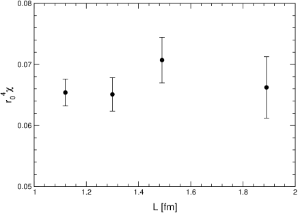
Figure 1: The topological susceptibility, in units of $r_{0}^{-4}$, as a function of the linear lattice size, in fm, at $\beta=6.0$.

Besides the statistical errors, the systematic uncertainties stem from finite-volume effects and from the extrapolation needed to reach the continuum limit.
The pure gauge theory has a mass gap, and therefore the topological susceptibility approaches the infinite-volume limit exponentially fast with $L$. Since the mass of the lightest glueball is around 1.5 GeV, finite-volume effects are expected to be far below our statistical errors as soon as $L\geq 1$ fm. In order to further verify that no sizeable finite-volume effects are present in our data, we simulated four lattices at $\beta=6.0$ but with different linear sizes $L=1.12,1.30,1.49,1.86$ fm. The results obtained for $\chi$ are shown in Fig. 1, where no dependence on $L$ is visible, hence confirming that finite-volume effects are below our statistical errors. In the large-volume regime the probability distribution of the topological charge is expected to be a Gaussian of the form Giusti et al. (2003b)

$$P_{Q}=\frac{1}{\sqrt{2\pi\langle Q^{2}\rangle}}e^{-\frac{Q^{2}}{2\langle Q^{2}\rangle}}\;.$$ (9)

We have checked that this formula describes all our data samples very well; for the lattice $D$, the results are shown in Fig. 2. Much higher statistics are required in order to highlight the deviations from a Gaussian distribution; higher momenta of the topological charge distribution measured on our data are all compatible with zero within large statistical errors.
As pointed out in the introduction, the topological susceptibility defined from the index of the Neuberger operator is not plagued by power divergences and does not require multiplicative renormalization. This is a distinctive feature of this approach, which is at variance with what happens for other definitions used in the past to compute $\chi$.

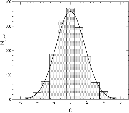
Figure 2: Histogram for the distribution of the topological charge $Q$ from the lattice $D$.

At finite lattice spacing, $\chi$ is affected by discretization effects starting at $O(a^{2})$, which are not universal, and, in our case, depend on the value of $s$ chosen to define the Neuberger operator. In order to compare results at different lattice spacings, and to extrapolate them to the continuum limit, we adopt $r_{0}$ as the reference scale; this choice is motivated by its precise determination in the range of $\beta$ explored in this work Guagnelli et al. (1998). The values of the adimensional quantity $r_{0}^{4}\chi$ that we obtain are reported in Table 1. Data, displayed in Fig. 3 as a function of $a^{2}/r_{0}^{2}$, show sizeable $O(a^{2})$ effects for both the $s=0.4$ and $s=0.0$ samples. For $\beta\leq 6.0$, the difference between the two discretizations is statistically significant. Within our statistical errors, and in the range where our simulations are performed, our results suggest a linear dependence in $a^{2}$. For the $s=0.4$ sample, the value of $\chi^{2}$ per degree of freedom, $\chi^{2}_{\mathrm{dof}}$, clearly disfavors a constant behavior, while a linear fit of the form

$$r_{0}^{4}\chi(s)=c_{0}+c_{1}(s)\Big{(}\frac{a}{r_{0}}\Big{)}^{2}$$ (10)

yields a value of $c_{0}=0.056(3)$ with $\chi^{2}_{\mathrm{dof}}\approx 0.79$. The quadratic fit in $a^{2}/r_{0}^{2}$ yields an extrapolated value compatible with that of the linear one, but with an error three times larger, and the coefficient of the quadratic term compatible with zero. For the $s=0.0$ sample, all three fits give good values of $\chi^{2}_{\mathrm{dof}}$, and for the linear one we obtain $c_{0}=0.064(4)$ with $\chi^{2}_{\mathrm{dof}}\approx 0.68$, which is compatible with the outcome of the same fit for $s=0.4$. The agreement between the two extrapolations indicates that we reached the scaling regime. This is confirmed by the compatibility of the results in the two data sets for $\beta>6.0$. A robust estimate of $\chi$ in the continuum limit can thus be obtained by performing a combined linear fit of the data. This fit gives a very good value of $\chi^{2}_{\mathrm{dof}}$ when all sets are included, and is very stable if some points at larger values of $a^{2}/r_{0}^{2}$ are removed. In particular a combined fit of all points with $a^{2}/r_{0}^{2}<0.05$ gives $c_{0}=0.059(3)$ with $\chi^{2}_{\mathrm{dof}}\approx 0.73$, and the error is expected to be Gaussian.

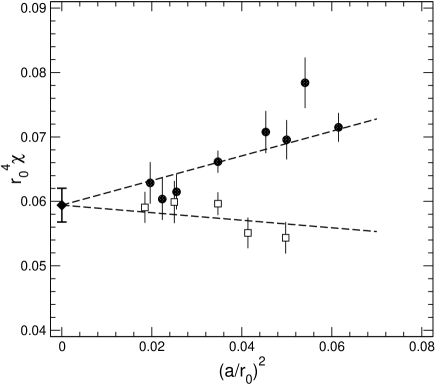
Figure 3: Continuum extrapolation of the adimensional product $r_{0}^{4}\chi$. The $s=0.0$ and $s=0.4$ data sets are represented by black circles and white squares respectively. The dashed lines represent the results of the combined fit described in the text. The filled diamond at $a=0$ is the extrapolated value in the continuum limit.

III Physical results

From the previous analysis, our best result for the topological susceptibility is the one obtained from a combined fit of the two sets of data with $a^{2}/r_{0}^{2}<0.05$:

$$r_{0}^{4}\chi=0.059\pm 0.003\,,$$ (11)

which is the main result of this work. Since $r_{0}$ is not directly accessible to experiments, we express our result in physical units by using the lattice determination of $r_{0}F_{K}=0.4146(94)$ in the pure gauge theory with valence quarks Garden et al. (2000) and, taking $F_{K}=160(2)$ MeV as an experimental input, we obtain

$$\chi=(191\pm 5\,\mathrm{MeV})^{4}\,,$$ (12)

which has to be compared with Veneziano (1979)

$$\frac{F_{\pi}^{2}}{6}\Big{(}m^{2}_{\eta}+m^{2}_{\eta^{\prime}}-2m^{2}_{K}\Big{)}\Big{|}_{\mathrm{exp}}\simeq(180\,\mathrm{MeV})^{4}\;.$$ (13)

Notice that, since Eq. (3) is valid only at the leading order in a $N_{\mathrm{f}}/N_{\mathrm{c}}$ expansion, the ambiguity in the conversion to physical units in the pure gauge theory is of the same order as the neglected terms.
Our result supports the fact that the bulk of the mass of the pseudoscalar singlet meson is generated by the anomaly through the Witten–Veneziano mechanism.

References

- Witten (1979) E. Witten, Nucl. Phys. B156, 269 (1979).
- Veneziano (1979) G. Veneziano, Nucl. Phys. B159, 213 (1979).
- Seiler and Stamatescu (1987) E. Seiler and I. O. Stamatescu (1987), mPI-PAE/PTh 10/87.
- Giusti et al. (2002) L. Giusti, G. C. Rossi, M. Testa, and G. Veneziano, Nucl. Phys. B628, 234 (2002), eprint hep-lat/0108009.
- Seiler (2002) E. Seiler, Phys. Lett. B525, 355 (2002), eprint hep-th/0111125.
- ’t Hooft (1974) G. ’t Hooft, Nucl. Phys. B72, 461 (1974).
- Kaplan (1992) D. B. Kaplan, Phys. Lett. B288, 342 (1992), eprint hep-lat/9206013.
- Narayanan and Neuberger (1993) R. Narayanan and H. Neuberger, Phys. Lett. B302, 62 (1993), eprint hep-lat/9212019.
- Narayanan and Neuberger (1994) R. Narayanan and H. Neuberger, Nucl. Phys. B412, 574 (1994), eprint hep-lat/9307006.
- Furman and Shamir (1995) V. Furman and Y. Shamir, Nucl. Phys. B439, 54 (1995), eprint hep-lat/9405004.
- Giusti (2003) L. Giusti, Nucl. Phys. Proc. Suppl. 119, 149 (2003), eprint hep-lat/0211009.
- Neuberger (1998a) H. Neuberger, Phys. Lett. B417, 141 (1998a), eprint hep-lat/9707022.
- Neuberger (1998b) H. Neuberger, Phys. Rev. D57, 5417 (1998b), eprint hep-lat/9710089.
- Neuberger (1998c) H. Neuberger, Phys. Lett. B427, 353 (1998c), eprint hep-lat/9801031.
- Ginsparg and Wilson (1982) P. H. Ginsparg and K. G. Wilson, Phys. Rev. D25, 2649 (1982).
- Luscher (1998) M. Luscher, Phys. Lett. B428, 342 (1998), eprint hep-lat/9802011.
- Fujikawa (1979) K. Fujikawa, Phys. Rev. Lett. 42, 1195 (1979).
- Hasenfratz et al. (1998) P. Hasenfratz, V. Laliena, and F. Niedermayer, Phys. Lett. B427, 125 (1998), eprint hep-lat/9801021.
- Giusti et al. (2004a) L. Giusti, G. C. Rossi, and M. Testa, Phys. Lett. B587, 157 (2004a), eprint hep-lat/0402027.
- Luscher (2004) M. Luscher (2004), eprint hep-th/0404034.
- Giusti et al. (2003a) L. Giusti, C. Hoelbling, M. Luscher, and H. Wittig, Comput. Phys. Commun. 153, 31 (2003a), eprint hep-lat/0212012.
- Bochicchio et al. (1984) M. Bochicchio, G. C. Rossi, M. Testa, and K. Yoshida, Phys. Lett. B149, 487 (1984).
- Smit and Vink (1987) J. Smit and J. C. Vink, Nucl. Phys. B286, 485 (1987).
- Berg (1981) B. Berg, Phys. Lett. B104, 475 (1981).
- Luscher (1982) M. Luscher, Commun. Math. Phys. 85, 39 (1982).
- Teper (1985) M. Teper, Phys. Lett. B162, 357 (1985).
- Alles et al. (1997) B. Alles, M. D’Elia, and A. Di Giacomo, Nucl. Phys. B494, 281 (1997), eprint hep-lat/9605013.
- de Forcrand et al. (1997) P. de Forcrand, M. Garcia Perez, J. E. Hetrick, and I.-O. Stamatescu (1997), eprint hep-lat/9802017.
- Hasenfratz and Nieter (1998) A. Hasenfratz and C. Nieter, Phys. Lett. B439, 366 (1998), eprint hep-lat/9806026.
- Lucini and Teper (2001) B. Lucini and M. Teper, JHEP 06, 050 (2001), eprint hep-lat/0103027.
- Ali Khan et al. (2001) A. Ali Khan et al. (CP-PACS), Phys. Rev. D64, 114501 (2001), eprint hep-lat/0106010.
- Del Debbio et al. (2002) L. Del Debbio, H. Panagopoulos, and E. Vicari, JHEP 08, 044 (2002), eprint hep-th/0204125.
- Edwards et al. (1999) R. G. Edwards, U. M. Heller, and R. Narayanan, Phys. Rev. D59, 094510 (1999), eprint hep-lat/9811030.
- DeGrand and Heller (2002) T. DeGrand and U. M. Heller (MILC), Phys. Rev. D65, 114501 (2002), eprint hep-lat/0202001.
- Gattringer et al. (2002) C. Gattringer, R. Hoffmann, and S. Schaefer, Phys. Lett. B535, 358 (2002), eprint hep-lat/0203013.
- Cundy et al. (2002) N. Cundy, M. Teper, and U. Wenger, Phys. Rev. D66, 094505 (2002), eprint hep-lat/0203030.
- Hasenfratz et al. (2002) P. Hasenfratz, S. Hauswirth, T. Jorg, F. Niedermayer, and K. Holland, Nucl. Phys. B643, 280 (2002), eprint hep-lat/0205010.
- Chiu and Hsieh (2003) T.-W. Chiu and T.-H. Hsieh, Nucl. Phys. B673, 217 (2003), eprint hep-lat/0305016.
- Del Debbio and Pica (2004) L. Del Debbio and C. Pica, JHEP 02, 003 (2004), eprint hep-lat/0309145.
- Giusti et al. (2003b) L. Giusti, M. Luscher, P. Weisz, and H. Wittig, JHEP 11, 023 (2003b), eprint hep-lat/0309189.
- Guagnelli et al. (1998) M. Guagnelli, R. Sommer, and H. Wittig (ALPHA), Nucl. Phys. B535, 389 (1998), eprint hep-lat/9806005.
- Garden et al. (2000) J. Garden, J. Heitger, R. Sommer, and H. Wittig (ALPHA), Nucl. Phys. B571, 237 (2000), [Erratum-ibid. B 679 (2004) 397], eprint hep-lat/9906013.
- Giusti et al. (2004b) L. Giusti, P. Hernandez, M. Laine, P. Weisz, and H. Wittig, JHEP 01, 003 (2004b), eprint hep-lat/0312012.