Towards a consistent noncommutative supersymmetric Yang-Mills theory: superfield covariant analysis.

Abstract

Commutative four dimensional supersymmetric Yang-Mills (SYM) is known to be renormalizable for ${\mathcal{N}}=1,2$, and finite for ${\mathcal{N}}=4$. However, in the noncommutative version of the model the UV/IR mechanism gives rise to infrared divergences which may spoil the perturbative expansion. In this work we pursue the study of the consistency of the ${\cal N}=1,2,4$ noncommutative supersymmetric Yang-Mills theory with gauge group $U(N)$ (NCSYM). We employ the covariant superfield framework to compute the one-loop corrections to the two- and three-point functions of the gauge superfield $V$. It is found that the cancellation of the harmful UV/IR infrared divergences only takes place in the fundamental representation of the gauge group. We argue that this is in agreement with the low energy limit of the open superstring in the presence of an external magnetic field. As expected, the planar sector of the two-point function of the $V$ superfield exhibits UV divergences. They are found to cancel, in the Feynman gauge, for the maximally extended ${\cal N}=4$ supersymmetric theory. This gives support to the belief that the ${\cal N}=4$ NCSYM theory is UV finite.

I Introduction

The four dimensional maximally extended supersymmetric Yang-Mills theory has recently been under intense scrutiny particularly due to its connection with the string/brane theory (see, for example, Kovacs and references therein). By contrast, studies on the renormalization properties of its noncommutative counterpart are more scarce. Some indications of its ultraviolet finiteness have already been given: using the background field formalism the one-loop four point function of the field strength has been computed Zanon1 ; Zanon2 and the finiteness of the model has been argued on the basis of the vanishing of the relevant beta function JJ . However, a direct calculation of the Green functions of the gauge potential $V$ within the superfield formalism is still lacking. As known, this study is essential to secure the ultraviolet finiteness of the higher order contributions to the effective action. Besides, the possible existence of nonintegrable infrared singularities, which can jeopardize the perturbative expansion, is particularly worrisome. Here we will furnish some further insight into these questions by providing an explicit calculation of the one-loop corrections to the two- and three-point vertex functions of the $V$ superfield. This work is the follow up of a recent paper of us dealing with the divergence structure of noncommutative supersymmetric QED₄ Ferrari1 . We shall use again the covariant superfield formalism to study the analogous problem for the ${\mathcal{N}}=1,2,4$ NCSYM theories in four space-time dimensions footnote1 . The reason for choosing $U(N)$ as the gauge group is based on the fact that it admits a simple noncommutative extension Chaichian ; footnote3 .

In Sec. II we present the action and the Feynman rules deriving from it, for the NCSYM theory. The one-loop corrections to the two-point function of the gauge superfield $V$ are computed and discussed in Sec. III. As will be seen, the fact that the gauge group is enforced to be in the fundamental representation warrants the cancellation of the leading UV/IR infrared divergences. We also demonstrate that, in the case ${\mathcal{N}}=4$, the planar sector of the one-loop corrections to the two-point function of the $V$ superfield turn out to be free of UV divergences. This supports the belief that, as in the commutative case, the ${\mathcal{N}}=4$ NCSYM theory is UV finite.

Consistency demands that the cancellation of the nonintegrable UV/IR infrared divergences should also take place in the fundamental representation for any n-point vertex function. This is, indeed, verified, in Sec. IV, for the leading UV/IR infrared divergences in the one-loop corrections to the three-point vertex function of the $V$ superfield. The conclusions and some final remarks are contained in Sec. V.

II The Action and Feynman rules of NCSYM

In ${\mathcal{N}}=1$ superspace, NCSYM in four space-time dimensions is described by the nonpolynomial action

$$S_{V}\,=\,-\,\frac{1}{2g^{2}}\int d^{8}z\,\operatorname{Tr}\,\left(e^{-gV}*D^{\alpha}e^{gV}\right)*\overline{D}^{2}\left(e^{-gV}*D_{\alpha}e^{gV}\right)\,,$$ (1)

where $g$ is the coupling constant, $V$ is a real Lie algebra valued vector superfield,

$$V\left(z\right)\,=\,V_{a}\left(z\right)\,T_{a}\,,$$ (2)

and the $T_{a},a=1,\cdots,N^{2}$, are the generators of $U(N)$ in the fundamental representation. They satisfy the algebra

$$\left[T_{a}\,,\,T_{b}\right]\,=\,i\,f_{abc}\,T_{c}\,.$$ (3)

Here, the $f_{abc}$’s are the structure constants of the gauge group. The generators are normalized according to

$$\operatorname{Tr}\left(T_{a}T_{b}\right)\,=\,\frac{1}{2}\,\delta_{ab}\,.$$ (4)

Furthermore, $D^{2}=1/2D^{\alpha}D_{\alpha}$, ${\bar{D}}^{2}=1/2{\bar{D}}_{\dot{\alpha}}{\bar{D}}^{\dot{\alpha}}$ and the Moyal product of field functions is defined as usual, i.e.,

$$\phi_{1}(x)\ast\phi_{2}(x)\,=\,\phi_{1}(x)\,exp\left(\frac{i}{2}\,\overleftarrow{\frac{\partial}{\partial x^{\mu}}}\,\Theta^{\mu\nu}\,\overrightarrow{\frac{\partial}{\partial x^{\nu}}}\right)\,\phi_{2}(x)$$

$$=\,\sum_{n=0}^{\infty}\,\left(\frac{i}{2}\right)^{n}\,\frac{1}{n!}\,\left[\partial_{\mu_{1}}\partial_{\mu_{2}}...\partial_{\mu_{n}}\,\phi_{1}(x)\right]\,\Theta^{\mu_{1}\nu_{1}}\Theta^{\mu_{2}\nu_{2}}...\Theta^{\mu_{n}\nu_{n}}\,\left[\partial_{\nu_{1}}\partial_{\nu_{2}}...\partial_{\nu_{n}}\,\phi_{2}(x)\right]\,,$$ (5)

where $\Theta^{\mu\nu}$ is the antisymmetric real constant matrix characterizing the noncommutativity of the underlying space-time footnote2 .

The gauge fixing is implemented by adding to the action $S_{V}$ the covariant term

$$S_{gf}\,=\,-\frac{a}{2}\int d^{8}z\,\operatorname{Tr}\,V\left\{D^{2},\overline{D}^{2}\right\}V\,,$$ (6)

where $a$ is a real constant labeling the gauge. The corresponding Faddeev-Popov determinant can be cast as

$$\Delta^{-1}\left[V\right]\,=\,\int\mathcal{D}c\,\mathcal{D}c^{\prime}\,\mathcal{D}\overline{c}\,\mathcal{D}\overline{c}^{\prime}\,e^{iS_{gh}[c,c^{\prime},{\bar{c}},{\bar{c}}^{\prime}]}\,.$$ (7)

The ghost fields $c,\overline{c}=c^{\dagger},c^{\prime},\overline{c}^{\prime}={c^{\prime}}^{\dagger}$ also take values in the Lie algebra, namely, $c(z)=c_{a}(z)T_{a}$ and so on. The explicit form for the ghost action is found to be

$$S_{gh}\,=\,i\,\left[c+\overline{c}\right]\,L_{\frac{g}{2}V}\,\left[-\left(c+\overline{c}\right)+\left(\coth L_{\frac{g}{2}V}\right)\left[\overline{c}-c\right]\right]\,,$$ (8)

where

$$L_{A}\left[B\right]\equiv\left[A,B\right]_{*}\,.$$ (9)

The ${\cal N}=2,4$ supersymmetric theories can be constructed by adding chiral matter superfields $\Phi^{i}\left(z\right)\,=\,\Phi^{i}_{a}\left(z\right)\,T_{a}$. The action describing a matter superfield interacting with the gauge superfield reads

$$S^{i}_{m}\,=\,\int d^{8}z\,\operatorname{Tr}\,\overline{\Phi}^{i}*e^{-gV}*\Phi^{i}*e^{gV}\,.$$ (10)

We remind the reader that the self-interaction among the chiral superfields $\Phi^{i},i=1,2,3$, entering the maximally extended ${\cal N}=4$ NCSYM model, may be entirely disregarded as far as the calculation of the one-loop corrections to the n-point vertex functions of the $V$ superfield is concerned. Because of this, the corresponding term has been omitted from the action.

From the quadratic part of the action $S_{V}+S_{gf}+S_{gh}+S_{m}$ one obtains the free propagators,

$$\Delta_{V_{a}V_{b}}(z_{1}-z_{2})\,=\,\delta_{ab}\,\frac{2i}{\Box}\,\left[1\,+\,(1-a)\,\frac{1}{\Box}\,\{D_{1}^{2},{\overline{D}}_{1}^{2}\}\right]\,\delta^{8}(z_{1}-z_{2})\,,$$ (11a)

$$\Delta_{{\overline{c}}_{a}c^{\prime}_{b}}(z_{1}-z_{2})\,=\,-\delta_{ab}\,\,\frac{2i}{\Box}\,D_{1}^{2}\,\overline{D}_{2}^{2}\,\delta^{8}(z_{1}-z_{2}),$$ (11b)

$$\Delta_{c_{a}{\overline{c}}^{\prime}_{b}}(z_{1}-z_{2})\,=\,\delta_{ab}\,\frac{2i}{\Box}\,{\overline{D}}_{1}^{2}\,{D}_{2}^{2}\,\delta^{8}(z_{1}-z_{2})\,,$$ (11c)

$$\Delta_{\Phi^{i}_{a}\overline{\Phi}^{j}_{b}}(z_{1}-z_{2})\,=\,-\,\delta^{ij}\,\delta_{ab}\,\,\frac{2i}{\Box}\,{\overline{D}}_{1}^{2}\,{D}_{2}^{2}\,\delta^{8}(z_{1}-z_{2})\,,$$ (11d)

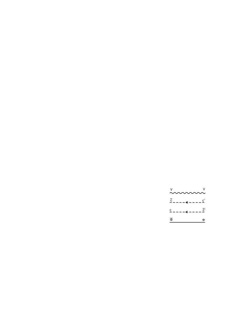
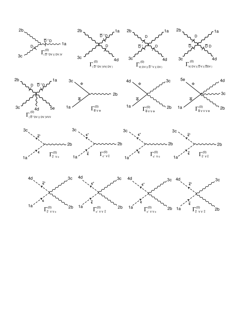
Figure 1: Free propagators.

Figure 2: Elementary vertices.

corresponding to the gauge, ghosts and matter superfields, respectively. They are depicted in Fig. 2. On the other hand, the interacting part of the total action enables us to find the elementary vertices needed for our calculations. They are displayed in Fig. 2. In an obvious notation,

$$\Gamma_{(\overline{D}^{2}DV_{a})V_{b}(DV_{c})}^{(0)}(k_{1},k_{2},k_{3})\,=\,\frac{ig}{2}\,\mathcal{V}_{3_{abc}}(k_{1},k_{2},k_{3})\,,$$ (12a)

$$\Gamma_{\overline{c}_{a}V_{b}c_{c}^{\prime}}^{(0)}(k_{1},k_{2},k_{3})\,=\,\Gamma_{c_{a}V_{b}\overline{c}_{c}^{\prime}}^{(0)}(k_{1},k_{2},k_{3})\,=\,\frac{ig}{2}\,\mathcal{V}_{3_{abc}}(k_{1},k_{2},k_{3})\,,$$ (12b)

$$\Gamma_{c_{a}V_{b}c_{c}^{\prime}}^{(0)}(k_{1},k_{2},k_{3})\,=\,\Gamma_{\overline{c}_{a}V_{b}\overline{c}_{c}^{\prime}}^{(0)}(k_{1},k_{2},k_{3})\,=\,-\frac{ig}{2}\,\mathcal{V}_{3_{abc}}(k_{1},k_{2},k_{3})\,,$$ (12c)

$$\Gamma_{\overline{\Phi}_{a}V_{b}\Phi_{c}}^{(0)}(k_{1},k_{2},k_{3})\,=\,-ig\,\mathcal{V}_{3_{abc}}(k_{1},k_{2},k_{3})\,,$$ (12d)

$$\Gamma_{(\overline{D}^{2}DV_{a})V_{b}V_{c}(DV_{d})}^{(0)}(k_{1},k_{2},k_{3},k_{4})\,=\,-\frac{ig^{2}}{24}\,\mathcal{V}_{4_{abcd}}^{(1)}(k_{1},k_{2},k_{3},k_{4})\,,$$ (12e)

$$\Gamma_{V_{a}DV_{b}DV_{c}(\overline{D}^{2}V_{d})}^{(0)}(k_{1},k_{2},k_{3},k_{4})\,=\,\frac{g^{2}}{4}\,\mathcal{V}_{4_{abcd}}^{(2)}(k_{1},k_{2},k_{3},k_{4})\,,$$ (12f)

$$\Gamma_{V_{a}DV_{b}\overline{D}DV_{c}(\overline{D}V_{d})}^{(0)}(k_{1},k_{2},k_{3},k_{4})\,=\,-\frac{g^{2}}{4}\,\mathcal{V}_{4_{abcd}}^{(2)}(k_{1},k_{2},k_{3},k_{4})\,,$$ (12g)

$$\Gamma_{c_{a}V_{b}V_{c}\overline{c}_{d}^{\prime}}^{(0)}(k_{1},k_{2},k_{3},k_{4})\,=\,\Gamma_{\overline{c}_{a}V_{b}V_{c}\overline{c}_{d}^{\prime}}^{(0)}(k_{1},k_{2},k_{3},k_{4})\,=\,-\frac{ig^{2}}{12}\,\mathcal{V}_{4_{abcd}}^{(1)}(k_{1},k_{2},k_{3},k_{4})\,,$$ (12h)

$$\Gamma_{\overline{c}_{a}V_{b}V_{c}c_{d}^{\prime}}^{(0)}(k_{1},k_{2},k_{3},k_{4})\,=\,\Gamma_{c_{a}V_{b}V_{c}c_{d}^{\prime}}^{(0)}(k_{1},k_{2},k_{3},k_{4})\,=\,+\frac{ig^{2}}{12}\,\mathcal{V}_{4_{abcd}}^{(1)}(k_{1},k_{2},k_{3},k_{4})\,,$$ (12i)

$$\Gamma_{\overline{\Phi}_{a}V_{b}V_{c}\Phi_{d}}^{(0)}(k_{1},k_{2},k_{3},k_{4})\,=\,\frac{ig^{2}}{2}\,\mathcal{V}_{4_{abcd}}^{(1)}(k_{1},k_{2},k_{3},k_{4})\,,$$ (12j)

$$\Gamma_{\overline{D}^{2}DV_{a}V_{b}V_{c}V_{d}DV_{e}}^{(0)}(k,p_{1},p_{2},p_{3},-k)\,=\,-\frac{ig^{3}}{24}\,\mathcal{V}_{5_{abcde}}(k,p_{1},p_{2},p_{3},-k)\,,$$ (12k)

$$\Gamma_{\overline{\Phi}_{a}V_{b}V_{c}V_{d}\Phi_{e}}^{(0)}(k,p_{1},p_{2},p_{3},-k)\,=\,-\frac{ig^{3}}{6}\,\mathcal{V}_{5_{abcde}}(k,p_{1},p_{2},p_{3},-k)\,.$$ (12l)

Here,

$$\mathcal{V}_{3_{abc}}(k_{1},k_{2},k_{3})\,\equiv\,e^{-ik_{2}\wedge k_{3}}\,A_{abc}-e^{ik_{2}\wedge k_{3}}\,A_{acb}\,,$$ (13a)

$$\mathcal{V}_{4_{abcd}}^{(1)}(k_{1},k_{2},k_{3},k_{4})\, \equiv \,e^{-i\left(k_{1}\wedge k_{2}+k_{3}\wedge k_{4}\right)}A_{abcd}-2e^{-i\left(k_{1}\wedge k_{2}+k_{4}\wedge k_{3}\right)}A_{abdc}$$ (13b)

$$+e^{-i\left(k_{1}\wedge k_{4}+k_{2}\wedge k_{3}\right)}A_{adbc}\,,$$

$$\mathcal{V}_{4_{abcd}}^{(2)}(k_{1},k_{2},k_{3},k_{4})\,\equiv\,\sin\left(k_{1}\wedge k_{2}\right)\left[e^{-ik_{3}\wedge k_{4}}A_{abcd}-e^{ik_{3}\wedge k_{4}}A_{adcb}\right]\,.$$ (13c)

As for ${\cal V}_{5_{abcde}}$ we shall only be needing ${\cal V}_{5}$ with two contracted indices, namely,

$$\mathcal{V}_{5_{abc}}(k,p_{1},p_{2},p_{3},-k)\,\equiv\,A_{dabcd}\,e^{-i\,p_{2}\wedge p_{3}}\,-\,A_{dabdc}\,e^{-i\,p_{2}\wedge p_{3}}-$$

$$-3\left[A_{dabdc}\,e^{-i\,p_{2}\wedge p_{3}}\,e^{2i\,k\wedge p_{3}}-A_{dadbc}\,e^{-i\,p_{2}\wedge p_{3}}\,e^{-2i\,k\wedge p_{1}}\right]\,,$$ (14)

where $\mathcal{V}_{5_{abc}}\equiv\mathcal{V}_{5_{dabcd}}$. The momenta are taken positive when entering the vertex and momentum conservation holds in all vertices. We have also introduced the definition

$$A_{a_{1}\cdots a_{n}}\,\equiv\,\operatorname{Tr}\left(T_{a_{1}}\cdots\,T_{a_{n}}\right)\,.$$ (15)

III One-loop corrections to the two-point vertex function of the gauge superfield

We turn now into computing the one-loop corrections to the two-point vertex function of the $V$ superfield, to be denoted by $\Gamma_{VV}^{(1)}$.

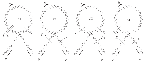
Figure 3: Graphs involving a quartic $V$ vertex.

In Fig. 3 we draw the contributions containing a quartic $V$-vertex, omitting those which vanish because of the $D$-algebra alone. According to the Feynman’s rules given in Sec. II, the amplitude associated with the graph $A1$ is found to read

$$\Gamma_{A1}\,=\,\left(-\frac{ig^{2}}{24}\right)\int\frac{d^{4}k}{\left(2\pi\right)^{4}}d^{4}\theta\,\left(F^{A1}\right)_{abcd}\left(-\,\delta^{ad}\frac{2i}{k^{2}}\right)\mathbb{D}_{\theta}^{A1}\,+\,\left(\mbox{sym}\right)\,,$$ (16)

where $F^{A1}$ is the phase factor originating from the Moyal product, $\mathbb{D}_{\theta}$ is the $\theta$-dependent part of the Feynman integrand and $\left(\mbox{sym}\right)$ means symmetrization over external legs which, in this case, implies in adding the diagram with $p\rightarrow-p$ and $b\leftrightarrow c$.

The calculation of $\mathbb{D}^{A1}_{\theta}$ is elementary and yields

$$\mathbb{D}_{\theta}^{A1}\,=\,-2\,V^{b}\left(p\right)V^{c}\left(-p\right)\,.$$ (17)

The phase factor can be computed by using Eqs. (12e) and (13b). Then, one ends up with

$$\Gamma_{A1}\,=\,\left(\frac{g^{2}}{3}\right)\,\int\frac{d^{4}k}{\left(2\pi\right)^{4}}d^{4}\theta\frac{1}{k^{2}}\left(F_{T}\right)_{bc}V^{b}\left(p\right)V^{c}\left(-p\right)\,,$$ (18)

where

$$\left(F_{T}\right)_{bc}\,=\,\left(A_{aabc}\,+\,A_{aacb}\right)\,-\,2cos\left(2k\wedge p\right)A_{abac}\,.$$ (19)

Notice that $\Gamma_{A1}$ appears to be, by power counting, quadratically UV divergent.

It will prove convenient to introduce the definition

$$Q_{0}\,=\,-\,g^{2}\,\int\frac{d^{4}k}{\left(2\pi\right)^{4}}d^{4}\theta\frac{1}{k^{2}}\left(F_{T}\right)_{bc}V^{b}\left(p\right)V^{c}\left(-p\right)\,,$$ (20)

which allows us to write

$$\Gamma_{A1}\,=\,-\frac{1}{3}Q_{0}\,.$$ (21)

According to Eq. (19), $F_{T}$ splits into planar (P) and non-planar (NP) parts. Correspondingly, $Q_{0}=Q_{0}^{P}+Q_{0}^{NP}$. The planar part $Q_{0}^{P}$ is indeed UV quadratically divergent, whereas $Q_{0}^{NP}$ develops a quadratic infrared pole through the UV/IR mechanism Minw .

Next on the line is the graph $A2$. It is not difficult to convince oneself that

$$\mathbb{D}_{\theta}^{A2}\,=\,-\frac{2}{k^{2}}\left(1-a\right)\,\overline{D}^{2}DV^{a}\left(p\right)\,DV^{d}\left(-p\right)\,,$$ (22)

and

$$\left(F^{A2}\right)_{abcd}\delta^{bc}\,=\,\left(A_{ccda}\,+\,A_{ccad}\right)-2e^{-2ik\wedge p}A_{acdc}\,,$$ (23)

lead to

$$\Gamma_{A2}\,=\,\left(1-a\right)\left(\frac{g^{2}}{6}\right)\int\frac{d^{4}k}{\left(2\pi\right)^{4}}d^{4}\theta\,\left[\left(F^{A2}\right)_{abcd}\delta^{bc}\right]\frac{1}{\left(k^{2}\right)^{2}}\,\overline{D}^{2}DV^{a}\left(p\right)\,DV^{d}\left(-p\right)\,+\,\left(\mbox{sym}\right)\,.$$ (24)

Hence, $\Gamma_{A2}$ is gauge dependent and contains, at most, logarithmic divergences. To implement the symmetrization with respect to the external legs we first invoke the relation

$$D^{\alpha}\overline{D}^{2}D_{\alpha}V\left(p\right)\,=\,\left(-\not\!p\,D\overline{D}+2D^{2}\overline{D}^{2}\right)V\left(p\right)\,=\,\left(+\not\!p\,\overline{D}D+2\overline{D}^{2}D^{2}\right)V\left(p\right)\,,$$ (25)

where $\not\!p\,D{\bar{D}}={\not\!p}_{\alpha{\dot{\alpha}}}\,D^{\alpha}{\bar{D}}^{{\dot{\alpha}}}$. Therefore, after realizing that $\left(F^{A2}\right)_{abcd}\delta^{bc}\,+\,\left(\mbox{sym}\right)\,=\,2\left(F_{T}\right)_{ad}$ one arrives at

$$\Gamma_{A2}\,=\,-\left(\frac{g^{2}}{3}\right)(1-a)\,\int\frac{d^{4}k}{\left(2\pi\right)^{4}}d^{4}\theta\left(F_{T}\right)_{ad}\frac{1}{\left(k^{2}\right)^{2}}V^{d}\left(-p\right)\left[-\not\!p\,D\overline{D}+2D^{2}\overline{D}^{2}\right]V^{a}\left(p\right)\,.$$ (26)

However, this expression does not yet appear as being symmetric under the exchange $p\rightarrow-p$ and $a\leftrightarrow d$. In order to explicitly exhibit such symmetry, we start by writing

$$\int d^{4}\theta\,V^{d}\left(-p\right)\left[-\not\!p\,D\overline{D}+2D^{2}\overline{D}^{2}\right]V^{a}\left(p\right)$$

$$=\frac{1}{2}\int d^{4}\theta\,V^{d}\left(-p\right)\left[-\not\!p\,D\overline{D}+2D^{2}\overline{D}^{2}\right]V^{a}\left(p\right)$$

$$+\,\frac{1}{2}\int d^{4}\theta\,V^{a}\left(p\right)\left[+\not\!p\,D\overline{D}+2D^{2}\overline{D}^{2}\right]V^{d}\left(-p\right)\,,$$ (27)

which, after integration by parts in the second term of the right hand side,

$$\int d^{4}\theta\,V^{d}\left(-p\right)\left[-\not\!p\,D\overline{D}+2D^{2}\overline{D}^{2}\right]V^{a}\left(p\right)$$

$$\,\,\,\,=\frac{1}{2}\int\,d^{4}\theta\,V^{d}\left(-p\right)\left[-\not\!p\left\{D,\overline{D}\right\}+2\left\{D^{2},\overline{D}^{2}\right\}\right]V^{a}\left(p\right)\,,$$ (28)

and since $\left\{D_{\alpha},{\bar{D}}_{{\dot{\alpha}}}\right\}V\left(p\right)={\not\!p}_{\alpha{\dot{\alpha}}}\,V\left(p\right)$ and ${\not\!p}_{\alpha{\dot{\alpha}}}\,{\not\!p}^{{\dot{\alpha}}\alpha}\,=\,2p^{2}$, becomes

$$\int d^{4}\theta\,V^{d}\left(-p\right)\left[-\not\!p\,D\overline{D}+2D^{2}\overline{D}^{2}\right]V^{a}\left(p\right)=\int d^{4}\theta\,V^{d}\left(-p\right)\left[-p^{2}+\left\{D^{2},\overline{D}^{2}\right\}\right]V^{a}\left(p\right)\,.$$ (29)

Thus, $\Gamma_{A2}$ can be cast

$$\Gamma_{A2}\,=\,\left(\frac{g^{2}}{3}\right)(1-a)\,\int\frac{d^{4}k}{\left(2\pi\right)^{4}}d^{4}\theta\left(F_{T}\right)_{ad}\frac{1}{\left(k^{2}\right)^{2}}V^{d}\left(-p\right)\left[p^{2}-\left\{D^{2},\overline{D}^{2}\right\}\right]V^{a}\left(p\right)\,,$$ (30)

which is obviously symmetric under the exchange $p\rightarrow-p$ and $a\leftrightarrow d$.

For future purposes, we introduce the definition

$$L_{0}\,=\,g^{2}\,\int\frac{d^{4}k}{\left(2\pi\right)^{4}}d^{4}\theta\left(F_{T}\right)_{ad}\frac{1}{\left(k^{2}\right)^{2}}V^{d}\left(-p\right)\left[p^{2}-\left\{D^{2},\overline{D}^{2}\right\}\right]V^{a}\left(p\right)\,,$$ (31)

in terms of which

$$\Gamma_{A2}\,=\,\frac{1}{3}\left(1-a\right)L_{0}\,.$$ (32)

As far as the graphs A3 and A4 are concerned, the $D$-algebra yields an integrand odd in $k$, in fact, proportional to $\not\!k/k^{4}$. On the other hand, the phase factor is, for both graphs, an even function of $k$. Hence, the symmetric $k$-integration leads to

$$\Gamma_{A3}\,=\,\Gamma_{A4}\,=\,0\,.$$ (33)

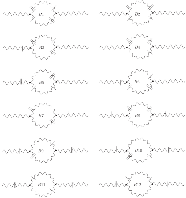
Figure 4: Contributions involving two trilinear $V$ vertices.

We next turn into the more complicated task of evaluating the diagrams involving two trilinear $V$ vertices, depicted in Fig. 4. There are many graphs to consider, differing among themselves in the distribution of the $D$-factors in each vertex. For reasons of space, we only present here the details of the calculation of the diagram $B1$. For the remaining ones, we shall merely quote the final results for the corresponding amplitudes.

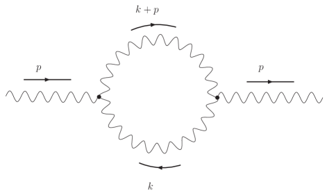
Figure 5: Momentum flow for the $V$-loop.

With the momentum flow indicated in Fig. 5, the Feynman rules applied to $B1$ lead to

$$\Gamma_{B1}\,=\,-\,\left(\frac{g^{2}}{2}\right)\int\frac{d^{4}k}{\left(2\pi\right)^{4}}d^{4}\theta_{1}d^{4}\theta_{2}\left(F^{B1}\right)_{abcdef}\delta^{af}\delta^{cd}\left[\frac{\left(i\right)^{2}}{k^{2}\left(k+p\right)^{2}}\right]\mathbb{D}_{\theta}^{B1}\,+\,\left(\mbox{sym}\right)\,.$$ (34)

As before, $\left(\mbox{sym}\right)$ means symmetrization over the external legs, i.e., adding the expression with $p\rightarrow-p$ and $b\leftrightarrow e$. By feeding the momenta in Fig. 5 into Eq. (13a) one obtains

$$\left(F^{B1}\right)_{abcdef}\delta^{af}\delta^{cd}\,=\,2\,\left(F_{L}\right)_{be}\,,$$ (35)

where

$$\left(F_{L}\right)_{be}\,\equiv\,A_{abc}A_{cea}-cos\left(2k\wedge p\right)A_{abc}A_{aec}\,.$$ (36)

The phase factor $\left(F_{L}\right)_{be}$, common to all diagrams in this topology, is symmetric in both momenta $k$ and $p$ as well as in color indices.

The $D$-algebra for the graph $\Gamma_{B1}$ is identical to that encountered for the corresponding diagram in the $U\left(1\right)$ case Ferrari1 . Hence, we write at once

$$\mathbb{D}_{\theta}^{B1}\,=\,-2\delta_{12}V_{2}^{e}\left(-p\right)\left[k^{2}\,+\,\not\!k\,D\,\overline{D}\,+\,D^{2}\overline{D}^{2}\right]V_{1}^{b}\left(p\right)\,.$$ (37)

By putting all the ingredients together we arrive at

$$\Gamma_{B1}\, = \,-\,2g^{2}\,\int\frac{d^{4}k}{\left(2\pi\right)^{4}}d^{4}\theta\left(F_{L}\right)_{be}\left\{k^{2}\left(\frac{V^{b}\left(p\right)V^{e}\left(-p\right)}{k^{2}\left(k+p\right)^{2}}+\frac{V^{e}\left(-p\right)V^{b}\left(p\right)}{k^{2}\left(k-p\right)^{2}}\right)\,\right.$$ (38)

$$+\,\not\!k\,\left(\frac{D\overline{D}V^{b}\left(p\right)V^{e}\left(-p\right)}{k^{2}\left(k+p\right)^{2}}+\frac{D\overline{D}V^{e}\left(-p\right)V^{b}\left(p\right)}{k^{2}\left(k-p\right)^{2}}\right)$$

$$\left.+\,\left(\frac{D^{2}\overline{D}^{2}V^{b}\left(p\right)V^{e}\left(-p\right)}{k^{2}\left(k+p\right)^{2}}+\frac{D^{2}\overline{D}^{2}V^{e}\left(-p\right)V^{b}\left(p\right)}{k^{2}\left(k-p\right)^{2}}\right)\right\}\,,$$

where the symmetrization has already been performed.

To isolate different powers of $k$ in the integrand of Eq. (38), we expand $\left(k\pm p\right)^{-2}$ around $p=0$, i.e.,

$$\frac{1}{\left(k\pm p\right)^{2}}\,=\,\frac{1}{k^{2}}\,\mp 2\frac{k\cdot p}{\left(k^{2}\right)^{2}}\,+\,\frac{4\left(k\cdot p\right)^{2}-k^{2}p^{2}}{\left(k^{2}\right)^{3}}\,+\,\cdots\,.$$ (39)

Then, after some manipulations envolving the $\theta$ integrals one finds

$$\Gamma_{B1}\, = \,-\,2g^{2}\,\int\frac{d^{4}k}{\left(2\pi\right)^{4}}d^{4}\theta\left(F_{L}\right)_{be}V^{e}\left(-p\right)\times$$ (40)

$$\times\left[\frac{2}{k^{2}}+\frac{4\left(k\cdot p\right)^{2}-k^{2}p^{2}}{\left(k^{2}\right)^{3}}-4\frac{\left(k\cdot p\right)^{2}}{\left(k^{2}\right)^{3}}+\frac{1}{\left(k^{2}\right)^{2}}\left\{D^{2},\overline{D}^{2}\right\}\right]V^{b}\left(p\right)\,+\,FT\,,$$

where “FT” is short for “finite terms”. To further simplify this expression we first write

$$\Gamma_{B1}\,=\,2\,Q_{1}\,-\,L_{1}\,+FT\,,$$ (41)

where

$$Q_{1}\,\equiv\,-\,2g^{2}\,\int\frac{d^{4}k}{\left(2\pi\right)^{4}}d^{4}\theta\frac{1}{k^{2}}\left(F_{L}\right)_{be}V^{b}\left(p\right)V^{e}\left(-p\right)\,$$ (42)

and

$$L_{1}\, = \,2g^{2}\,\int\frac{d^{4}k}{\left(2\pi\right)^{4}}d^{4}\theta\left(F_{L}\right)_{be}\frac{1}{\left(k^{2}\right)^{2}}V^{e}\left(-p\right)$$ (43)

$$\times \left[\frac{4\left(k\cdot p\right)^{2}-k^{2}p^{2}}{\left(k^{2}\right)}-4\frac{\left(k\cdot p\right)^{2}}{\left(k^{2}\right)}+\left\{D^{2},\overline{D}^{2}\right\}\right]V^{b}\left(p\right)\,.$$

From observation follows that $Q_{1}$ and $L_{1}$ are, respectively, quadratically and logarithmically divergent by power counting. Furthermore, for the planar part of $L_{1}$ one can take advantage of

$$\int d^{4}k\,k_{\mu}k_{\nu}f\left(k^{2}\right)\,=\,\frac{1}{4}g_{\mu\nu}\int d^{4}k\,k^{2}f\left(k^{2}\right)$$ (44)

to write

$$L_{1}^{P}\,\equiv\,-\,2g^{2}\,\int\frac{d^{4}k}{\left(2\pi\right)^{4}}d^{4}\theta\frac{1}{\left(k^{2}\right)^{2}}\left(F_{L}^{P}\right)_{be}V^{e}\left(-p\right)\left(p^{2}-\left\{D^{2},\overline{D}^{2}\right\}\right)V^{b}\left(p\right)\,.$$ (45)

The nonplanar part $L_{1}^{NP}$ develops a logarithmic UV/IR infrared pole which, for being harmless, can be lumped into “FT”. To summarize, we may cast $\Gamma_{B1}$ in the following final form

$$\Gamma_{B1}\,=\,2Q_{1}-L_{1}^{P}\,+FT\,.$$ (46)

The planar part of $Q_{1}$ is quadratically UV divergent, while the nonplanar one develops a quadratic UV/IR infrared pole. As can be seen from (45), $L_{1}^{P}$ is logarithmically UV divergent.

For the remaining diagrams in Fig. 4 we found

$$\Gamma_{B2}\,=\,-2Q_{1},\hskip 28.45274pt\Gamma_{B3}\,=\,L_{2}^{P}-2L_{1}^{P}+FT,\hskip 28.45274pt\Gamma_{B4}\,=\,0,$$

$$\Gamma_{B5}\,=\,2L_{1}^{P}+FT,\hskip 28.45274pt\Gamma_{B6}\,=\,-2L_{1}^{P}+FT,\hskip 28.45274pt\Gamma_{B7}\,=\,L_{1}^{P}+FT,$$

$$\Gamma_{B8}\,=\,-2\left(1-a\right)L_{1}^{P},\hskip 28.45274pt\Gamma_{B9}\,=\,-2aL_{1}^{P}+FT,\hskip 28.45274pt\Gamma_{B10}\,=\,-2aL_{1}^{P}+FT,$$

$$\Gamma_{B11}\,=\,FT,\hskip 28.45274pt\Gamma_{B12}\,=\,FT\,,$$ (47)

where

$$L_{2}^{P}\,\equiv\,-\,2g^{2}\,\int\frac{d^{4}k}{\left(2\pi\right)^{4}}d^{4}\theta\frac{p^{2}}{\left(k^{2}\right)^{2}}\left(F_{L}^{P}\right)_{be}V^{e}\left(-p\right)V^{b}\left(p\right)\,.$$ (48)

By adding up Eqs. (21), (32), (33), (46), (47), one arrives at

$$\Gamma_{A}\,+\,\Gamma_{B}\,=\,-\frac{1}{3}Q_{0}\,+\,\frac{1}{3}(1-a)L_{0}\,-\,2(2+a)L_{1}^{P}\,+\,L_{2}^{P}\,+\,FT\,.$$ (49)

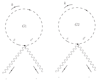
Figure 6: Ghost tadpole contributions.

Ghost loop contributions to $\Gamma_{VV}^{\left(1\right)}$ involving a quartic vertex arise from the graphs depicted in Fig. 6. A straightforward application of the Feynman rules yields

$$\Gamma_{G1}\,=\,\left(-1\right)\left(\frac{ig^{2}}{12}\right)\int\frac{d^{4}k}{\left(2\pi\right)^{4}}d^{4}\theta\,\left(F^{G1}\right)_{abcd}\left(\delta^{ad}\frac{2i}{k^{2}}\right)\mathbb{D}_{\theta}^{G1}\,+\,\left(\mbox{sym}\right)\,,$$ (50)

and

$$\Gamma_{G2}\,=\,\left(-1\right)\left(-\frac{ig^{2}}{12}\right)\int\frac{d^{4}k}{\left(2\pi\right)^{4}}d^{4}\theta\,\left(F^{G2}\right)_{abcd}\left(-\delta^{ad}\frac{2i}{k^{2}}\right)\mathbb{D}_{\theta}^{G2}\,+\,\left(\mbox{sym}\right)\,.$$ (51)

In view of $F^{G1}=F^{G2}$ and $\mathbb{D}_{\theta}^{G1}=\mathbb{D}_{\theta}^{G2}$ one concludes that $\Gamma_{G1}=\Gamma_{G2}$ and, hence,

$$\Gamma_{G1}+\Gamma_{G2}\,=\,-\frac{2}{3}Q_{0}\,.$$ (52)

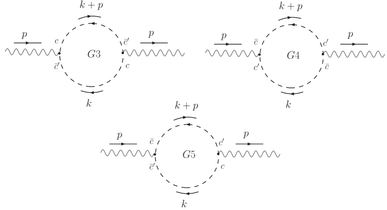
Figure 7: Diagrams involving a ghost loop.

The diagrams containing a ghost loop with two trilinear vertices are indicated in Fig. 7. Both $\Gamma_{G3}$ and $\Gamma_{G4}$ are very similar to $\Gamma_{B1}$. Indeed, $\Gamma_{G3}\,=\,\Gamma_{G4}$ and $\Gamma_{G3}+\Gamma_{G4}=\Gamma_{B1}$. Therefore, according to Eq. (46),

$$\Gamma_{G3}+\Gamma_{G4}\,=\,2Q_{1}-L_{1}^{P}\,+FT\,.$$ (53)

It remains to compute the graph $G5$. Since

$$\mathbb{D}_{\theta}^{G5}\,=\,D^{2}\overline{D}^{2}\delta_{12}D^{2}\overline{D}^{2}\delta_{12}V^{b}\left(p\right)V^{e}\left(-p\right)\,=\,\delta_{12}\overline{D}^{2}D^{2}V^{b}\left(p\right)V^{e}\left(-p\right)\,,$$ (54)

it can at most be logarithmically divergent. The topological weight for this diagram is $2$. Then,

$$\Gamma_{G5}\,=\,L_{3}^{P}\,+FT\,,$$ (55)

where

$$L_{3}^{P}\,=\,2g^{2}\,\int\frac{d^{4}k}{\left(2\pi\right)^{4}}d^{4}\theta_{1}\frac{1}{\left(k^{2}\right)}\left(F_{L}^{P}\right)_{be}V^{e}\left(-p\right)\left\{\overline{D}^{2},D^{2}\right\}V^{b}\left(p\right)\,.$$ (56)

The total contribution of ghost loops to $\Gamma_{VV}^{(1)}$ is obtained from Eqs. (52), (53), (55), and amounts to

$$\Gamma_{G}\,=\,-\frac{2}{3}Q_{1}\,-\,L_{1}^{P}\,+\,L_{3}^{P}\,+\,FT\,.$$ (57)

One should notice that Eqs. (45), (48), and (56) imply that

$$L_{1}^{P}\,=\,L_{2}^{P}\,+\,L_{3}^{P}\,.$$ (58)

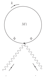
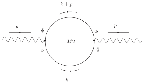
Figure 8: Matter contributions.

We address now the calculation of the matter contributions to the two-point vertex function of the $V$ superfield. The relevant diagrams for each matter superfield are depicted in Fig. 8. Up to numerical factors, their evaluation is just as for the corresponding ghost graphs, since $c,c^{\prime}$ ($\overline{c},\overline{c}^{\prime}$) and $\Phi^{i}$ ($\overline{\Phi}^{i}$) are both chiral (antichiral) superfields. Thus, for diagram $M1$ one finds

$$\Gamma_{M1}\,=\,2Q_{0}\,.$$ (59)

As for $M2$, one has $\Gamma_{M2}\,=\,-4\Gamma_{G3}\,=\,-2\Gamma_{B1}$, i.e.,

$$\Gamma_{M2}\,=\,-4Q_{1}+2L_{1}^{P}\,+FT\,$$ (60)

and, therefore,

$$\Gamma_{M1}+\Gamma_{M2}\,=\,2\left(Q_{0}\,-\,2Q_{1}\,+\,L_{1}^{P}\right)\,+\,FT\,$$ (61)

is the one-loop correction to $\Gamma_{VV}$ contributed by each chiral matter superfield. In particular, for the maximally extended (${\cal N}=4$) NCSYM theory,

$$\Gamma_{M}\,=\,3\times(\Gamma_{M1}+\Gamma_{M2})\,.$$ (62)

Now we are able to discuss the structure of divergences of $\Gamma_{VV}^{(1)}$. Let us first focus on its planar part, which contains all the UV divergences. Quadratic UV divergences are washed out by dimensional regularization, while linear ones are killed by symmetric integration. All that is left are logarithmic UV divergences and UV finite terms. For ${\cal N}=1,2$, these divergences must be renormalized. As for ${\cal N}=4$, it turns out that

$$\left[\Gamma_{VV}^{(1)}\right]_{\textrm{logarithmic UV}}\,=\,2(1\,-\,a)\,L_{1}^{P}\,+\,\frac{1}{3}(1-a)L_{0}\,,$$ (63)

as seen from Eqs. (49), (57), (62), and (58). As in the commutative case Storey1 ; Storey2 , the maximally extended supersymmetric theory turns out to be free of ultraviolet divergences in the Feynman gauge ($a=1$).

We concentrate next into studying the nonplanar part of $\Gamma_{VV}^{(1)}$, which due to the noncommutativity is UV finite but develops infrared poles through the UV/IR mechanism. As for the $U\left(1\right)$ model Ferrari1 , the phase factor originated from the noncommutativity is always an even function of $k$ and, hence, there can be no linear UV/IR infrared divergences. Then, the only harmful UV/IR poles are the quadratic ones, contained in $Q_{1}$ and $Q_{0}$. For the pure gauge sector one finds (see Eqs. (49) and (57))

$$\left[\Gamma_{A}^{NP}+\Gamma_{B}^{NP}+\Gamma_{G}^{NP}\right]_{\textrm{quadratic UV/IR}}\,=\,-Q_{0}^{NP}+2Q_{1}^{NP}\,,$$ (64)

while, for each chiral matter superfield (see Eq. (61)),

$$\left[\Gamma_{M1}^{NP}+\Gamma_{M2}^{NP}\right]_{\textrm{quadratic UV/IR}}\,=\,2Q_{0}^{NP}-4Q_{1}^{NP}\,.$$ (65)

Therefore, the quadratic UV/IR infrared divergences cancel both for the ${\cal N}=1$ as well as for the extended supersymmetric NCSYM if

$$\frac{1}{2}Q_{0}^{NP}\,=\,Q_{1}^{NP}\,,$$ (66)

which, in view of the definitions in Eqs.(20) and (42), demands that

$$\int\frac{d^{4}k}{\left(2\pi\right)^{4}}\left(F_{T}^{NP}\right)_{be}\int d^{4}\theta V^{b}\left(p\right)V^{e}\left(-p\right)\,=\,4\,\int\frac{d^{4}k}{\left(2\pi\right)^{4}}\left(F_{L}^{NP}\right)_{be}\int d^{4}\theta V^{b}\left(p\right)V^{e}\left(-p\right)\,.$$ (67)

According to Eqs. (19) and (36), a sufficient condition for Eq. (67) to hold is

$$\operatorname{Tr}\left(T_{a}T_{b}T_{a}T_{e}\right)\,=\,2\,\operatorname{Tr}\left(T_{a}T_{b}T_{c}\right)\,\operatorname{Tr}\left(T_{a}T_{e}T_{c}\right)\,.$$ (68)

For the fundamental representation of $U(N)$, the set of generators is complete and, therefore Penati ,

$$(T_{a})_{ij}(T_{a})_{kl}\,=\,\frac{1}{2}\,\delta_{il}\delta_{jk}\,,$$ (69)

which guarantees that Eq. (68) is, in fact, verified.

IV Leading UV/IR infrared divergences in the one-loop corrections to the three-point vertex function

In connection with higher-point vertex functions, it is natural to expect that the cancellation of the nonintegrable UV/IR infrared singularities will require further conditions involving the traces of the group generators, like in Eq. (68). The natural question is whether these conditions will be verified by the generators in the fundamental representation of the gauge group $U(N)$. A throughout investigation to provide a full answer to this question is clearly impracticable but we may, nevertheless, start to clarify the situation by looking at the one-loop corrections to the three-point vertex function of the gauge superfield $V$, hereafter to be denoted by $\Gamma_{VVV}^{(1)}$. For reasons of simplicity, we shall restrict here to study the leading (quadratic by power counting) divergences.

The diagrams contributing to $\Gamma_{VVV}^{(1)}$ and involving a vector loop are generically depicted in Fig. 9. We shall first address the supergraph $V1$ involving the quintic vertex of the gauge superfield. The corresponding amplitude is found to read

$$\Gamma_{V1}\,=\,\left(-\frac{ig^{3}}{24}\right)\int\frac{d^{4}k}{\left(2\pi\right)^{4}}\mathbb{D}_{\theta}\,\left(F_{V1}\right)_{abcde}\left(-\delta^{ae}\frac{2i}{k^{2}}\right)\mathbb{D}_{\theta}^{G}\,+\,\left(\mbox{sym}\right)\,.$$ (70)

The phase factor $F_{V1}$ can be calculated from Eq. (14). Since the objects of interest are the leading UV/IR infrared singularities, we single out the nonplanar part of $F_{V1}$ which is proportional to

$$e^{-i\,p_{2}\wedge p_{3}}\,\left[A_{dabdc}\,e^{2i\,k\wedge p_{3}}-A_{dadbc}\,e^{-2i\,k\wedge p_{1}}\right]\,.$$ (71)

With the help of

$$\int\frac{d^{4}k}{\left(2\pi\right)^{4}}\frac{e^{2ik\wedge p}}{k^{2}}=\frac{1}{4\pi^{2}p\circ p}\,$$ (72)

and after total symmetrization with respect to the external momenta and color indices, one concludes that $\Gamma_{V1}$ does not contain quadratic UV/IR infrared divergences.

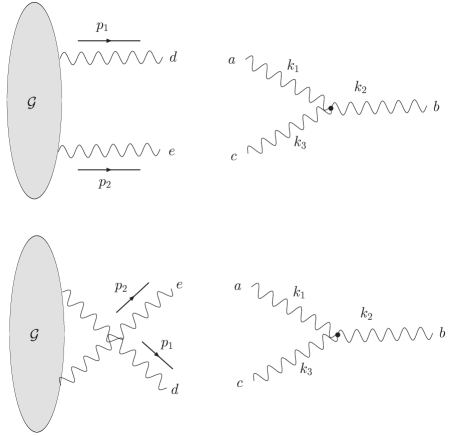
Figure 10: Antisymmetric property of the triple vertex $\bar{D}^{2}DV^{a}V^{b}DV^{c}$.

Leading UV/IR infrared divergences arising from the remaining diagrams in Fig. 9 also vanish as consequence of a simple property involving the triple vertex $\bar{D}^{2}DV^{a}V^{b}DV^{c}$: the exchange of two legs contracted with the field derivative factors contained in the just mentioned vertex, implies in an overall change of sign in the corresponding amplitude. To understand why this happens, let us consider some (sub)supergraph ${\cal G}$ with two legs $V^{d}(p_{1})$ and $V^{e}(p_{2})$ to be contracted with the $\bar{D}^{2}DV^{a}V^{b}DV^{c}$ vertex (see Fig. 10). The amplitude associated with ${\cal G}$ will schematically be given by

$$(\ldots)_{de}V^{d}(p_{1})V^{e}(p_{2}).$$ (73)

We observe that only the terms involving derivates in the triple $V$ vertex are to be contracted with $V^{d}(p_{1})$ and $V^{e}(p_{2})$. Indeed, if doing otherwise we would not be looking at a diagram containing leading divergences. As indicated in Fig. 10, there are two ways to perform such contraction:

(i) $V^{d}$ is contracted with $V^{a}$ and $V^{e}$ with $V^{c}$. The resulting amplitude reads

$$[\ldots]_{de}\delta^{da}\delta^{ec}[e^{ip_{1}\wedge p_{2}}A_{abc}-e^{-ip_{1}\wedge p_{2}}A_{acb}]\,=\,[\ldots]_{de}[e^{ip_{1}\wedge p_{2}}A_{dbe}-e^{-ip_{1}\wedge p_{2}}A_{deb}]\,.$$ (74)

(ii) $V^{d}$ is contracted with $V^{c}$ and $V^{e}$ with $V^{a}$. In this case the amplitude turns out to be

$$[\ldots]_{de}\delta^{dc}\delta^{ea}[e^{ip_{2}\wedge p_{1}}A_{abc}-e^{-ip_{2}\wedge p_{1}}A_{acb}]\,=\,-\,[\ldots]_{de}[e^{ip_{1}\wedge p_{2}}A_{dbe}-e^{-ip_{1}\wedge p_{2}}A_{deb}]\,.$$ (75)

Clearly, the sign difference between Eqs. (74) and (75) is at the root of the mechanism of cancellation for the leading divergent contributions arising from diagrams $V2$ and $V3$ in Fig. 9.

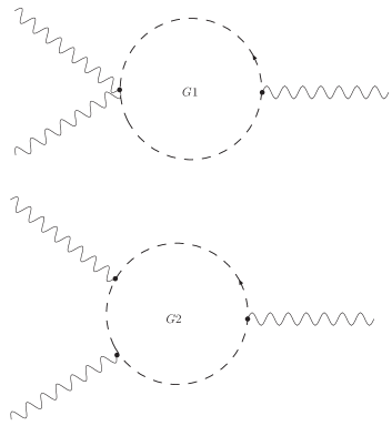
Figure 11: Ghost loops contributions to $\Gamma_{VVV}^{(1)}$.

As for the ghost loop contributions, depicted in Fig. 11, the cancellation of the leading UV/IR infrared singularities is a direct consequence of the Feynman rules given in Sec. II.

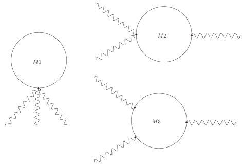
Figure 12: Matter loops contributions to $\Gamma_{VVV}^{(1)}$.

We finally turn into considering the matter loop contributions to $\Gamma_{VVV}^{(1)}$, shown in Fig. 12. The amplitude associated with $M1$ is proportional to the one corresponding to diagram $V1$ in Fig. 9 and, hence, its nonplanar part vanishes.

The phase factor corresponding to the supergraph $M2$, involving one triple and one quartic matter vertices, is given by

$$\left(F_{M2}\right)_{eabdecd} = e^{-i(2k\wedge p_{3}+p_{1}\wedge p_{2})}A_{eabd}A_{ecd}-e^{-i(-2k\wedge p_{3}+p_{1}\wedge p_{2})}A_{dabe}A_{dce}$$ (76)

$$- 2e^{-i(-2k\wedge p_{1}-p_{1}\wedge p_{2})}A_{eadb}A_{ecd}+2e^{-i(2k\wedge p_{2}-p_{1}\wedge p_{2})}A_{eadb}A_{dce}\,.$$

The sum of the first two terms turns out to be an odd function of the integration momentum $k$ and, therefore, does not contribute to the leading divergences. Hence, the nonplanar piece of the amplitude containing the leading UV/IR infrared divergences is proportional to

$$\int\frac{d^{4}k}{\left(2\pi\right)^{4}} \frac{1}{k^{2}}\left(e^{-i(2k\wedge p_{1}-p_{1}\wedge p_{2})}A_{eadb}A_{ecd}-e^{-i(2k\wedge p_{2}-p_{1}\wedge p_{2})}A_{eadb}A_{dce}\right)\,+\,(\mbox{sym})\,=$$ (77)

$$=\,\frac{1}{4\pi^{2}}\,e^{i\,p_{1}\wedge p_{2}}\left(\frac{A_{eadb}A_{ecd}}{p_{1}\circ p_{1}}-\frac{A_{eadb}A_{dce}}{p_{2}\circ p_{2}}\right)\,+\,(\mbox{sym})\,,$$

which can be cast

$$\frac{i}{2\pi^{2}}\sin(p_{1}\wedge p_{2})\,\Big{[} \frac{1}{p_{1}\circ p_{1}}(A_{eadb}A_{ecd}-A_{eadc}A_{ebd})\,+\,\frac{1}{p_{2}\circ p_{2}}(A_{ebdc}A_{ead}-A_{ebda}A_{ecd})$$ (78)

$$+\,\frac{1}{p_{3}\circ p_{3}}(A_{ecda}A_{ebd}-A_{ecdb}A_{ead})\,\Big{]}\,.$$

It is easy to see that this last expression vanishes if and only if

$$\operatorname{Tr}(T_{d}T_{a}T_{e}T_{b})\operatorname{Tr}(T_{d}T_{c}T_{e})\,=\,\operatorname{Tr}(T_{d}T_{a}T_{e}T_{c})\operatorname{Tr}(T_{d}T_{b}T_{e})\,.$$ (79)

Again, Eq. (69) suffices to secure that (79) holds.

Finally, the supergraph $M3$, involving three matter vertices, does not yield leading UV/IR infrared singularities due to a mechanism similar to the one described in connection with diagram $V2$ in Fig. 9.

We then conclude that the restriction to the fundamental group representation protects the quantum corrections to the vertex functions of the $V$ superfield from the appearance of nonintegrable UV/IR infrared divergences. We emphasize that the same condition is required for the $U(N)$ to become an operational gauge group at the classical level Chaichian .

V Summary

In this work we studied the structure of the divergences of the two- and three-point vertex functions of the $V$ gauge superfield in the NCSYM theory in four spacetime dimensions with the aim of establishing the consistency of the model.

In the planar sector, we found logarithmic UV divergences which cancel in the ${\cal N}=4$ extended supersymmetric theory in the Feynman gauge. We confirm the belief that ${\cal N}=4$ NCSYM theory is finite JJ .

As for the nonplanar sector, the restriction of the group generators to be in the fundamental representation turned out to be essential to guarantee the cancellation of the leading UV/IR infrared divergences in the two- and three-point vertex functions of $V$. Therefore, one may hope that the UV/IR mechanism will not jeopardize the perturbative expansion at higher-loop orders.

We close this paper by pointing out that the results in this work are in agreement with the understanding of noncommutative supersymmetric field theories as the low energy limit of open superstrings in the presence of an external magnetic field SW . We first recall that the matrices of the gauge groups associated with the open type I superstring (SST I) are restricted to the fundamental representations of $U(N)$, $SO(N)$ and $USp(N)$ footnote4 . The low energy limit of SST I is ${\cal N}=1$ SYM, in ten space-time dimensions, and reduces to ${\cal N}=4$ SYM when six dimensions are compactified. As known, these field theories are insensitive to the dimension of the gauge group matrices. On the other hand, when a background magnetic field is turned on the low energy limit of the SST I is a noncommutative supersymmetric gauge field theory which only exists in the fundamental representation of the gauge group matrices. In fact, the above restriction turns out to be essential for the quantum corrections to be free of the harmful UV/IR infrared singularities.

Acknowledgements. This work was partially supported by Fundação de Amparo à Pesquisa do Estado de São Paulo (FAPESP) and Conselho Nacional de Desenvolvimento Científico e Tecnológico (CNPq). H. O. G. and V. O. R. also acknowledge support from PRONEX under contract CNPq 66.2002/1998-99. A. Yu. Petrov has been supported by FAPESP, project No. 00/12671-7.

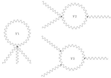
Figure 9: Vector loop contributions to $\Gamma_{VVV}^{(1)}$.