Moduli-Space Approximation for BPS Brane-Worlds

Moduli-Space Approximation for BPS Brane-Worlds

Gonzalo A. Palma and Anne-Christine Davis

Department of Applied Mathematics and Theoretical Physics,
Center for Mathematical Sciences, University of Cambridge,
Wilberforce Road, Cambridge CB3 0WA,
United Kingdom.

Abstract

We develop the moduli-space approximation for the low energy regime of BPS-branes with a bulk scalar field to obtain an effective four-dimensional action describing the system. An arbitrary BPS potential is used and account is taken of the presence of matter in the branes and small supersymmetry breaking terms. The resulting effective theory is a bi-scalar tensor theory of gravity. In this theory, the scalar degrees of freedom can be stabilized naturally without the introduction of additional mechanisms other than the appropriate BPS potential. We place observational constraints on the shape of the potential and the global configuration of branes.

Brane-worlds scenarios are an interesting theoretical possibility to address many questions and problems of low and high energy physics [1]. In these models the construction of four dimensional effective theories has proved particularly useful to describe the physics of branes at the low energy regime. It has been shown [2] that these effective theories have much in common with multi-scalar-tensor theories of gravity, where the inter-brane distance plays the role of a scalar degree of freedom. This is the case, for example, of the Randall-Sundrum model [3] where the radion field emerges in the four dimensional description.

In this letter we construct the moduli-space approximation for the low energy regime of a general BPS brane-world model, which has been motivated as a supersymmetric extension of the Randall–Sundrum model [4] (see [5] for phenomenological motivations). The model consists of a five-dimensional bulk space with a scalar field $\psi$, bounded by two branes, $\sigma_{1}$ and $\sigma_{2}$. The main property of this system is a special boundary condition that holds between the branes and the bulk fields, which allows the branes to be located anywhere in the background without obstruction. In particular, a special relation exists between the scalar field potential $U(\psi)$, defined in the bulk, and the brane tensions $U_{B}(\psi^{1})$ and $U_{B}(\psi^{2})$ defined at the position of the branes. This is the BPS condition. Due to the difficulties of this setup, in previous works, only the special case of dilatonic branes have been considered, where the BPS potential has the form $U_{B}\propto e^{\alpha\psi}$. Here we consider an arbitrary potential $U_{B}$.

We now introduce the system in more detail. Let us consider a 5-dimensional manifold $M$ with the special topology $M=\sigma\times S^{1}/Z_{2}$, where $\sigma$ is a fixed 4-dimensional lorentzian manifold without boundaries and $S^{1}/Z_{2}$ is the orbifold constructed from the 1-dimensional circle with points identified through a $Z_{2}$-symmetry. The manifold $M$ is bounded by two branes located at the fixed points of $S^{1}/Z_{2}$. Let us denote the brane-surfaces by $\sigma_{1}$ and $\sigma_{2}$ respectively and the space bounded by the branes as the bulk space. In our model there is a bulk scalar field $\psi$ living in $M$ with boundary values, $\psi^{1}$ and $\psi^{2}$, at the branes, with bulk potential $\mathcal{U}(\psi)$ and brane tensions $\mathcal{V}_{1}(\psi^{1})$ and $\mathcal{V}_{2}(\psi^{2})$ (which are potentials for the boundary values $\psi^{1}$ and $\psi^{2}$). Additionally, we will consider the existence of matter fields $\Psi_{1}$ and $\Psi_{2}$ confined to the branes. Figure 1 shows a schematic representation of the present configuration.

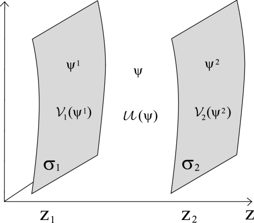
Figure 1: Schematic representation of the 5-dimensional brane configuration. In the bulk there is a scalar field $\psi$ with a bulk potential $\mathcal{U}(\psi)$. Additionally, the bulk-space is bounded by branes, $\sigma_{1}$ and $\sigma_{2}$, with tensions given by $\mathcal{V}_{1}(\psi^{1})$ and $\mathcal{V}_{2}(\psi^{2})$ respectively, where $\psi^{1}$ and $\psi^{2}$ are the boundary values of $\psi$.

Given the present topology, it is appropriate to introduce foliations with a coordinate system $x^{\mu}$ describing $\sigma$ (as well as the branes $\sigma_{1}$ and $\sigma_{2}$) where $\mu=0,\ldots,3$. Additionally, we can introduce a coordinate $z$ describing the $S^{1}/Z_{2}$ orbifold and parameterizing the foliations. With this decomposition the following form of the line element can be used to describe $M$ (the gaussian normal coordinate system):

$$ds^{2}=N^{2}dz^{2}+g_{\mu\nu}dx^{\mu}dx^{\nu}\!.$$ (1)

Here $N$ is the lapse function for the extra dimensional coordinate $z$ and, therefore, it can be defined up to a gauge choice. Additionally, $g_{\mu\nu}$ is the pullback of the induced metric on the 4–dimensional foliations, with the $(-,+,+,+)$ signature. The branes, $\sigma_{1}$ and $\sigma_{2}$, are located at the fixed points of the $S^{1}/Z_{2}$ orbifold, denoted by $z=z_{1}$ and $z=z_{2}$. Without loss of generality, we take $z_{1}<z_{2}$. The total action of the system is

$$S_{\mathrm{tot}}=S_{\mathrm{G}}+S_{\mathrm{\psi}}+S_{\mathrm{BR}},$$ (2)

where $S_{\mathrm{G}}$ is the action describing the pure gravitational part and is given by $S_{\mathrm{G}}=S_{\mathrm{EH}}+S_{\mathrm{GH}}$, with $S_{\mathrm{EH}}$ the Einstein–Hilbert action and $S_{\mathrm{GH}}$ the Gibbons–Hawking boundary terms. In the present parameterization:

$$S_{\mathrm{G}}=\frac{1}{2\kappa_{5}^{2}}\int_{M}\!\!\!\!dz\,d^{\,4}x\sqrt{-g}\,N\big{(}R-K_{\mu\nu}K^{\mu\nu}+K^{2}\big{)},$$ (3)

where $R$ is the four-dimensional Ricci scalar constructed from $g_{\mu\nu}$, and $\kappa_{5}^{2}=8\pi G_{5}$, with $G_{5}$ the five-dimensional Newton’s constant. Additionally, $K_{\mu\nu}=g_{\mu\nu}^{\prime}/2N$ is the extrinsic curvature of the foliations and $K$ its trace (the prime denotes derivatives in terms of $z$, that is ${}^{\prime}=\partial_{z}$, and covariant derivatives, $\nabla_{\mu}$, are constructed from the induced metric $g_{\mu\nu}$ in the standard way). The action for the bulk scalar field, $S_{\psi}$, can be written in the form

$$S_{\psi} = -\frac{3}{8\kappa_{5}^{2}}\int_{M}\!\!\!\!dz\,d^{\,4}x\sqrt{-g}\,N\big{[}(\psi^{\prime}/N)^{2}+(\partial\psi)^{2}+\mathcal{U}(\psi)\big{]}+S_{\psi}^{\,1}+S_{\psi}^{\,2},$$ (4)

where $S_{\psi}^{\,1}$ and $S_{\psi}^{\,2}$ are boundary terms given by

$$S_{\psi}^{\,1} = -\frac{3}{2\kappa_{5}^{2}}\int_{\sigma_{1}}\!\!\!d^{4}x\sqrt{-g}\,\mathcal{V}_{1}(\psi^{1}),$$ (5)

$$S_{\psi}^{\,2} = +\frac{3}{2\kappa_{5}^{2}}\int_{\sigma_{2}}\!\!\!d^{4}x\sqrt{-g}\,\mathcal{V}_{2}(\psi^{2}),$$ (6)

at the respective positions, $z_{1}$ and $z_{2}$ and $\mathcal{U}(\psi)$ is the bulk scalar field potential, while $\mathcal{V}_{1}(\psi^{1})$ and $\mathcal{V}_{2}(\psi^{2})$ are boundary potentials. Finally, for the matter fields confined to the branes, we shall consider the standard action:

$$S_{\mathrm{BR}}=S_{1}[\Psi_{1},g_{\mu\nu}(z_{1})]+S_{2}[\Psi_{2},g_{\mu\nu}(z_{2})],$$ (7)

where $\Psi_{1}$ and $\Psi_{2}$ denote the respective matter fields, and $g_{\mu\nu}(z_{a})$ is the induced metric at position $z_{a}$. In the present case (BPS-configurations), we shall consider the following general form for the potentials: $\mathcal{U}=U+u$, $\mathcal{V}_{1}=U_{B}+v_{1}$ and $\mathcal{V}_{2}=U_{B}+v_{2}$, where $U$ and $U_{B}$ are the bulk and brane superpotentials, and the potentials $u$, $v_{1}$ and $v_{2}$ are such that $|u|\ll|U|$ and $|v_{1}|,|v_{2}|\ll|U_{B}|$. In this way, the system is dominated by the superpotentials $U$ and $U_{B}$. The most important characteristic of this class of system is the relation between $U$ and $U_{B}$ (the BPS-relation), given by:

$$U=\left(\partial_{\psi}U_{B}\right)^{2}-U_{B}^{2}.$$ (8)

This specific configuration, when the potentials $u,v_{1},v_{2}=0$ and no fields other than the bulk scalar field are present, is the BPS configuration. When $U_{B}$ is the constant potential, the Randall–Sundrum model is recovered with a bulk cosmological constant $\Lambda_{5}=(3/8)U=-(3/8)\,U_{B}^{2}$. The presence of the potentials $u$, $v_{1}$ and $v_{2}$ are generally expected from supersymmetry breaking effects.

To develop the moduli space approximation of the present system, we need to know its static vacuum solution. To this extent, consider a bulk scalar field $\psi_{0}$ and gravitational fields $N_{0}$ and $\tilde{g}_{\mu\nu}(x)$, such that:

$$\partial_{\mu}\psi_{0}=0,\,\,\quad\partial_{\mu}N_{0}=0,\,\,\quad\mathrm{and}\,\,\quad\tilde{G}_{\mu\nu}=0,$$ (9)

(where $\tilde{G}_{\mu\nu}$ is the four-dimensional Einstein tensor constructed from $\tilde{g}_{\mu\nu}$) and also consider a metric $g_{\mu\nu}=\omega^{2}(z)\tilde{g}_{\mu\nu}$ so that the $z$ dependence of $g_{\mu\nu}$ is only contained in the warp factor $\omega(z)$. Then, let us assume that these fields satisfy the following two relations:

$$\frac{\omega_{0}^{\prime}}{\omega_{0}}=-\frac{1}{4}N_{0}U_{B},\quad\quad\psi_{0}^{\prime}=N_{0}\frac{\partial U_{B}}{\partial\psi_{0}}.$$ (10)

These are the BPS relations, which agree with the boundary conditions for the bulk fields in the absence of matter and supersymmetry breaking terms. On the other hand, when they hold, then $\psi_{0}$, $N_{0}$ and $g_{\mu\nu}=\omega^{2}(z)\tilde{g}_{\mu\nu}$ solve the entire system of equations of motion. This important fact constitutes one of the main properties of BPS-systems, and means that the branes can be arbitrarily located anywhere in the background, without obstruction. It should be clear, though, that when matter is allowed to exist in the branes the boundary conditions will not continue being solutions to the equations of motion, and the static configuration will not be possible; the presence of matter in the branes drives the system to a cosmological evolution.

In the static vacuum solution expressed through the equations in (10), the dependence of the lapse function $N_{0}$, in terms of $z$ is completely arbitrary (though it must be restricted to be positive) and its precise form will correspond to a gauge choice. Let us assume that $\psi_{0}(z)$ has boundary values:

$$\psi^{1}=\psi_{0}(z_{1}),\quad\mathrm{and}\quad\psi^{2}=\psi_{0}(z_{2}).$$ (11)

Since we are interested in the static vacuum solution, $\psi^{1}$ and $\psi^{2}$ are just constants. The precise form of $\psi_{0}(z)$, as a function of $z$, depends on the form of $U_{B}(\psi)$ and the gauge choice for $N_{0}$. However, it is not difficult to see that $\psi^{1}$ and $\psi^{2}$ are the only degrees of freedom, jointly with $\tilde{g}_{\mu\nu}$, necessary to specify the BPS state of the system. That is, given a gauge choice $N_{0}$, we have: $\psi_{0}=\psi_{0}(z,\psi^{1},\psi^{2})$ and $N_{0}=N_{0}(z,\psi^{1},\psi^{2})$. Moreover, it is possible to show that by virtue of the relations in (10), the solution $\psi_{0}$ must be monotonic in term of $z$ in the complete bulk space [6]. Therefore, the change of variable $dz=N_{0}^{-1}\left(\partial_{\psi_{0}}U_{B}\right)^{-1}\!d\psi_{0}$ can be used to parameterize the fifth dimension in terms of $\psi_{0}$, and the boundary values $\psi^{1}$ and $\psi^{2}$ specify the positions of the branes.

Observe additionally, from eq. (10), that $\omega_{0}(z)$ can be expressed in terms of $\psi_{0}(z)$ in a gauge independent way:

$$\omega_{0}(z) = \exp\left[-\frac{1}{4}\int_{\psi^{1}}^{\psi_{0}(z)}\!\!\alpha^{-1}(\psi)\,d\psi\right],$$ (12)

$$\alpha(\psi) = \frac{1}{U_{B}}\frac{\partial U_{B}}{\partial\psi}.$$ (13)

In the last equations we have normalized the solution $\omega_{0}(z)$ in such a way that the induced metric to the first brane is $\tilde{g}_{\mu\nu}$. The induced metric on the second brane is, therefore, conformally related to the first brane, with a warp factor $\omega_{0}(z_{2})$.

We now proceed to compute the moduli-space approximation. First of all, varying the action $S_{\mathrm{tot}}$ in terms of $N$, we deduce the following equation of motion:

$$K^{2}-K_{\mu\nu}K^{\mu\nu}=R+\frac{3}{4}\bigg{[}\frac{1}{N^{2}}(\psi^{\prime})^{2}-(\partial\psi)^{2}-\mathcal{U}\bigg{]}.$$ (14)

This result can be inserted back into the action (2):

$$S_{\mathrm{tot}} = \frac{1}{\kappa_{5}^{2}}\int_{M}\!\!dz\,d^{\,4}x\sqrt{-g}\,N\Big{[}R-\frac{3}{4}(\partial\psi)^{2}-\frac{3}{4}\mathcal{U}\Big{]}+S^{1}_{\psi}+S^{2}_{\psi}+S_{\mathrm{BR}}.$$ (15)

We can now exploit the static vacuum solution. As we mentioned, when matter is present in the branes as well as supersymmetry breaking terms, the system becomes dynamical. Hence, the boundary fields $\psi^{1}$ and $\psi^{2}$ and the metric $\tilde{g}_{\mu\nu}$ no longer satisfy vacuum equations of motion; instead we insert $\psi_{0}$, $N_{0}$ and $g_{\mu\nu}=\omega^{2}\tilde{g}_{\mu\nu}$ as ansatzs into the action (15). That is, the positions of the branes, which are parameterized by the moduli $\psi^{1}$ and $\psi^{2}$, are being perturbed by the matter content of the branes. Thus we obtain the following action for $\psi^{1}$, $\psi^{2}$ and $\tilde{g}_{\mu\nu}$:

$$S_{\mathrm{tot}} = \frac{1}{\kappa_{5}^{2}}\int_{M}\!\!dz\,d^{\,4}x\sqrt{-\tilde{g}}\,N_{0}\omega_{0}^{4}\Big{[}\omega_{0}^{-2}\tilde{R}-6\omega_{0}^{-3}\Box\omega_{0}-\frac{3}{4}\omega_{0}^{-2}(\partial\psi_{0})^{2}-\frac{3}{4}u\Big{]}$$ (16)

$$-\frac{3}{2\kappa_{5}^{2}}\int_{\sigma_{1}}\!\!\!d^{4}x\sqrt{-g}\,v_{1}+\frac{3}{2\kappa_{5}^{2}}\int_{\sigma_{2}}\!\!\!d^{4}x\sqrt{-g}\,v_{2}+S_{\mathrm{BR}},$$

where the BPS relation (10) was used to evaluate some terms at the boundaries. To obtain a more conventional form for the action in terms of $\psi^{1}$, $\psi^{2}$ and $\tilde{g}_{\mu\nu}$ we need to integrate along the fifth dimension. To do this it is necessary to note the following identity from eq. (10):

$$\partial_{\mu}(N_{0}\omega_{0})=-N_{0}\alpha_{0}\omega_{0}\partial_{\mu}\psi_{0}-\frac{4}{U_{B}}(\partial_{\mu}\omega_{0})^{\prime}.$$ (17)

This expression allows us to rewrite the term $6(\partial\omega_{0})^{2}+(3/4)(\partial\psi_{0})^{2}$, present in the action (16), as:

$$6\omega_{0}^{-1}\Box\omega_{0}+\frac{3}{4}(\partial\psi_{0})^{2}=12(N_{0}\omega_{0}^{4})^{-1}\left[\frac{1}{U_{B}}(\partial\omega_{0})^{2}\right]^{\prime}+\frac{3}{4}\omega_{0}^{-2}\alpha_{0}^{2}\alpha_{1}^{-2}(\partial\psi^{1})^{2},$$ (18)

where $\alpha_{0}=\alpha(\psi_{0})$ and $\alpha_{1}=\alpha(\psi^{1})$. Now, using the parameterization $dz=N_{0}^{-1}\left(\partial_{\psi_{0}}U_{B}\right)^{-1}\!d\psi_{0}$ to integrate along the fifth dimension and the boundary values $\psi^{1}(x)$ and $\psi^{2}(x)$ to evaluate at the positions of the branes $z_{1}$ and $z_{2}$, we arrive at the following effective theory:

$$S = \frac{1}{k\kappa_{5}^{2}}\int d^{4}x\sqrt{-\tilde{g}}\bigg{[}\Omega^{2}\tilde{R}-\frac{3}{4}\tilde{g}^{\mu\nu}\gamma_{ab}\partial_{\mu}\psi^{a}\partial_{\nu}\psi^{b}-\frac{3}{4}V\bigg{]}$$ (19)

$$+S_{1}[\Psi_{1},\tilde{g}_{\mu\nu}]+S_{2}[\Psi_{2},\omega^{2}(z_{2})\tilde{g}_{\mu\nu}],\qquad$$

where the index $a$ labels the positions $1$ and $2$. The conformal factor $\Omega^{2}$ in front of the Ricci scalar $\tilde{R}$, is given by:

$$\Omega^{2}=k\int_{\psi^{1}}^{\psi^{2}}\!\!\!\!\!d\psi\left(\frac{\partial U_{B}}{\partial\psi}\right)^{-1}\!\!\!\omega^{2},$$ (20)

where $\omega$ is given by equation (12). The coefficient $k$ is an arbitrary positive constant with dimensions of inverse length to make $\Omega^{2}$ dimensionless. The symmetric matrix $\gamma_{ab}$ depends on the moduli fields, and can be regarded as the metric of the moduli space in a sigma model approach. Additionally, the elements of $\gamma_{ab}$ are given by:

$$\gamma_{11} = \alpha_{1}^{-2}\left[\frac{k}{U_{B}(\psi^{1})}-\frac{1}{2}\Omega^{2}\right],$$ (21)

$$\gamma_{22} = \alpha_{2}^{-2}\frac{\omega^{2}(z_{2})k}{U_{B}(\psi^{2})},$$ (22)

$$\gamma_{12} = -\alpha_{1}^{-1}\alpha_{2}^{-1}\frac{\omega^{2}(z_{2})k}{U_{B}(\psi^{2})},$$ (23)

with $\gamma_{21}=\gamma_{12}$. Finally, we have also defined an effective potential $V$ which depends linearly on the supersymmetry breaking potentials $u$, $v_{1}$ and $v_{2}$. This is defined as:

$$V=\frac{k}{2}\int^{\psi^{2}}_{\psi^{1}}\!\!\!\!\!d\psi\left(\frac{\partial U_{B}}{\partial\psi}\right)^{-1}\!\!\!\omega^{4}\,u-2k\left[\omega^{4}(z_{2})v_{2}-v_{1}\right].$$ (24)

The generic form of the deduced theory is of a bi-scalar tensor theory of gravity, with the two scalar degrees given by $\psi^{1}$ and $\psi^{2}$. Note that in equation (19) the Newton’s constant depends on the moduli fields. This theory can be rewritten in the Einstein frame where the Newton’s constant is independent of the moduli. By considering the conformal transformation $\tilde{g}_{\mu\nu}\rightarrow g_{\mu\nu}=\Omega^{2}\tilde{g}_{\mu\nu}$ we are then left with the following action:

$$S = \frac{1}{k\kappa_{5}^{2}}\int d^{4}x\sqrt{-g}\bigg{[}R-\frac{3}{4}g^{\mu\nu}\gamma_{ab}\partial_{\mu}\psi^{a}\partial_{\nu}\psi^{b}-\frac{3}{4}V\bigg{]}$$ (25)

$$+S_{1}[\Psi_{1},A_{1}^{2}g_{\mu\nu}]+S_{2}[\Psi_{2},A_{2}^{2}g_{\mu\nu}],$$

where now the sigma model metric $\gamma_{ab}$ is given by:

$$\gamma_{11} = 2\alpha_{1}^{-2}\frac{k^{2}A_{1}^{4}}{U_{B}^{2}(\psi^{1})}\bigg{[}1-\frac{1}{2k}U_{B}(\psi^{1})A_{1}^{-2}\bigg{]},$$ (26)

$$\gamma_{22} = 2\alpha_{2}^{-2}\frac{k^{2}A_{2}^{4}}{U_{B}^{2}(\psi^{2})}\bigg{[}1+\frac{1}{2k}U_{B}(\psi^{2})A_{2}^{-2}\bigg{]},$$ (27)

$$\gamma_{12} = -2\alpha_{1}\alpha_{2}\frac{k^{2}A_{1}^{2}A_{2}^{2}}{U_{B}(\psi^{1})U_{B}(\psi^{2})}.$$ (28)

It is possible to show that in this frame $\gamma_{ab}$ is a positive definite metric. Additionally, we have defined the quantities $A_{1}$ and $A_{2}$ (which are functions of the moduli) to be $A_{1}^{-2}=\Omega^{2}$ and $A_{2}^{-2}=\Omega^{2}\omega^{-2}(z_{2})$, or explicitly:

$$A_{1}^{-2}=k\!\!\int_{\psi^{1}}^{\psi^{2}}\!\!\!\!\!d\psi\left(\frac{\partial U_{B}}{\partial\psi}\right)^{\!\!-1}\!\!\!\!\!\exp\left[-\frac{1}{2}\int_{\psi^{1}}^{\psi}\!\!\!\!\alpha^{-1}d\psi\right],\qquad$$ (29)

$$A_{2}^{-2}=k\!\!\int_{\psi^{1}}^{\psi^{2}}\!\!\!\!\!d\psi\left(\frac{\partial U_{B}}{\partial\psi}\right)^{\!\!-1}\!\!\!\!\!\exp\left[-\frac{1}{2}\int_{\psi^{2}}^{\psi}\!\!\!\!\alpha^{-1}d\psi\right].\qquad$$ (30)

Also, the potential $V$ is now found to be:

$$V = \frac{k}{2}\Omega^{-4}\int^{\psi^{2}}_{\psi^{1}}\!\!\!\!\!d\psi\left(\frac{\partial U_{B}}{\partial\psi}\right)^{-1}\!\!\!\omega^{4}\,u-2k\left[A_{2}^{4}v_{2}-A_{1}^{4}v_{1}\right].$$ (31)

Our effective action can be used extensively for the study of this class of systems. It can also be obtained in the projective approach, when a perturbative method is used to analyze the five-dimensional equations of motion [6]. Additionally, it agrees with previous computations, where the specific case of dilatonic branes, $U_{B}\propto e^{\alpha\psi}$, was considered [7]. To obtain the next order in the moduli space approximation, we should consider linear perturbations about the vacuum solution. That is, we should consider: $g_{\mu\nu}=\omega_{0}^{2}\left(\tilde{g}_{\mu\nu}+h_{\mu\nu}\right)$, $\psi=\psi_{0}+\varphi$ and $N=N_{0}\,e^{\phi}$, with the linear fields satisfying $|h_{\mu\nu}|\ll|\tilde{g}_{\mu\nu}|$, $|\varphi|\ll|\psi_{0}|$ and $|\phi|\ll 1$. The study of these linear perturbation was considered in detail in [6].

When the cosmological evolution of branes is considered it is possible show that the branes are driven by the matter content in them. In particular, the first brane, $\sigma_{1}$, is driven towards the minimum of the BPS potential, while the second brane, $\sigma_{2}$, is driven towards the maximum [6]. This allows the system to fall in a stable configuration. For example, we can compute the Post Newtonian Eddington coefficient $\gamma$ which is constrained by measurements of the deflection of radio waves by the Sun to be $\gamma=1+(2.1\pm 2.3)\times 10^{-5}$ [8]. The parameter $\gamma$ is found to be:

$$1-\gamma\simeq\frac{2}{3}\left[1-\frac{1}{2k}U_{B}(\psi^{1})A_{1}^{-2}\right].$$ (32)

This is a very important result: since the branes must be near the extremes of the BPS potential, observational measurements constrain the global configuration of the brane system, as well as the shape of the potential.

Summarizing, in this paper we have developed the moduli-space approximation of the low energy regime of BPS brane-world models. As a result, an effective 4-dimensional system of equations have been obtained. At this order, the metrics of both branes are conformally related, and the complete theory corresponds to a bi-scalar tensor theory of gravity [equation (25)]. Our effective theory allows the study of this class of models within the approach and usual techniques of multi-scalar tensor theories [9]. For instance, we have indicated that the moduli fields can be stabilized, and that the system can be constrained by observations.

We are grateful to Philippe Brax and Carsten van de Bruck for useful comments and discussions. This work is supported in part by PPARC and MIDEPLAN (GAP).

References

• [1] For comprehensive reviews see: Ph. Brax and C. van de Bruck, Class. Quantum Grav. 20, R201 (2003); D. Langlois, Prog. Theor. Phys. Suppl. 148, 181 (2003); R. Maartens, gr-qc/0312059, Living Rev. Rel. (to appear); Ph. Brax, C. van de Bruck and A.C. Davis, hep-th/0404011, Rept. Prog. Phys. (to appear).
• [2] J. Garriga and T. Tanaka, Phys. Rev. Lett. 84, 2778 (2000); T. Chiba, Phys. Rev. D 62, 021502 (2000); T. Tanaka and X Montes, Nucl. Phys. B 582, 259 (2000); P. Binetruy, C. Deffayet and D. Langlois, Nucl. Phys. B 615, 219 (2001); Ph. Brax, C. van de Bruck, A. C. Davis and C. S. Rhodes, Phys. Rev. D 65, 121501 (2002).
• [3] L. Randall and R. Sundrum, Phys. Rev. Lett. 83 3370 (1999); Phys. Rev. Lett. 83 4690 (1999).
• [4] E. Bergshoeff, R. Kallosh and A.V. Proeyen, JHEP 0010, 033 (2000); P. Binetruy, J.M. Cline and C. Grojean, Phys. Lett. B 489, 403 (2000); Ph. Brax and A. C. Davis, Phys. Lett. B 497, 289 (2001); JHEP 0105, 007 (2001); C. Csaki, J. Erlich, C. Grojean, T.J. Hollowood, Nucl. Phys. B 584, 359 (2000); D. Youm, Nucl. Phys. B 596, 289 (2001).
• [5] E.E. Flanagan, S.H.H. Tye and I. Wasserman, Phys. Lett. B 522, 155 (2001); O. DeWolfe, D.Z. Freedman, S.S. Gubser and A. Karch, Phys. Rev. D 62, 046008 (2000).
• [6] Gonzalo A. Palma and Anne-Christine Davis, hep-th/0406091.
• [7] Ph. Brax, C. van de Bruck, A. C. Davis and C. S. Rhodes, Phys. Rev. D 67, 023512 (2003).
• [8] T. M. Eubanks et al., Am. Phys. Soc., Abstract K 11.05 (1997); C. Will, Living Rev. Rel. 4, 4 (2001); B. Bertotti, L. Iess and P. Tortora, Nature 425, 374 (2003).
• [9] T. Damour and G. Esposito-Farese, Class. Quantum Grav. 9, 2093 (1992); T. Damour, Phys. Rev. Lett. 70, 2217 (1993).