Logarithmic Conformal Field Theories and Strings in Changing Backgrounds

Abstract

I review a particular class of physical applications of Logarithmic Conformal Field Theory in strings propagating in changing (not necessarily conformal) backgrounds, namely D-brane recoil in flat or time-dependent cosmological backgrounds. The role of recoil logarithmic vertex operators as non-conformal deformations requiring in some cases Liouville dressing is pointed out. It is also argued that, although in the case of non-supersymmetric recoil deformations the representation of target time as a Liouville zero mode may lead to non-linear quantum mechanics for stringy defects, such non-linearities disappear (or, at least, are strongly suppressed) after world-sheet supersymmetrization. A possible link is therefore suggested between (world-sheet) supersymmetry and linearity of quantum mechanics in this framework.

1 Introduction

In this article, as a tribute to Ian Kogan, I would like to review some work that I have done partly with him, in connection with some physical applications of Logarithmic Conformal Field Theory (LCFT) to strings propagating in changing backgrounds. Such a situation is encountered, for instance, when a macroscopic number of closed strings hits a D-particle, embedded in a $d$-dimensional space time, and forces the D-particle to recoil via an impulse [1, 2]. Equivalently, pairs of logarithmic operators may occur in some (nearly conformal) cosmological backgrounds of string theory, such as late times Robertson-Walker (RW) cosmology [3]. In the first case, the logarithmic pair consists of the velocity and the position of the non-relativistic recoiling brane defect, while in the second example it is the cosmic velocity and acceleration that enter in a logarithmic fashion.

In the context of non-supersymmetric D-particle recoil an interesting situation arises. The target time dynamics of the recoiling defects can be described in terms of the (irreversible) flow of a renormalization-group (RG) scale on the world-sheet of the underlying $\sigma$-model describing the stringy excitations of the recoiling D-particle. This leads to non-linear terms in the associated “evolution equation” based on the identification of target time with such a RG scale [4, 5]. The latter is nothing other than the zero mode of the associated Liouville $\sigma$-model field required for restoration of the conformal invariance, which was broken by the recoil/impulse (non marginal) deformations. Upon going to the supersymmetric case, however, which is realized via appropriately supersymmetrized recoil operators, such non-linearities disappear (or at least are strongly suppressed), and the associated evolution dynamics for the D-particles is that of a linear Schrödinger-like quantum mechanics. This may have some interesting implications in linking supersymmetry (of some form) to linearity of quantum mechanics. The key result in our analysis was that world-sheet leading ultraviolet (UV) divergences in an appropriate Zamolodchikov metric of the recoil operators, which in the non-supersymmetric (bosonic) string case lead to diffusion like terms in the quantum evolution, and hence to non-linearities, cancel out in the supersymmetric case, thereby leading to ordinary Schrödinger evolution under the identification of the world-sheet RG scale with target time. This latter result provides a highly non-trivial consistency check of the above identification, at least in this specific context.

Logarithmic conformal field theories [6, 7] have been attracting a lot of attention in recent years because of their diverse range of applications, from condensed matter models of disorder [8, 9] to applications involving gravitational dressing of two-dimensional field theories [10], a general analysis of target space symmetries in string theory [11], D-brane recoil [1, 2], $AdS$ backgrounds in string theory and also M-theory [13], as well as $PP$-wave backgrounds in string theory[14] (see [15] for reviews and more exhaustive lists of references). They lie on the border between conformally invariant and general renormalizable field theories in two dimensions. A logarithmic conformal field theory is characterized by the property that its correlation functions differ from the standard conformal field theoretic ones by terms which contain logarithmic branch cuts. Nevertheless, it is a limiting case of an ordinary conformal field theory which is still compatible with conformal invariance and which can still be classified to a certain extent by means of conformal data.

The current understanding of logarithmic conformal field theories lacks the depth and generality that characterizes the conventional conformally invariant field theories. Most of the analyses so far pertain to specific models, and usually to those involving free field realizations. Nevertheless, some general properties of logarithmic conformal field theories are now very well understood. For example, an important deviation from standard conformal field theory is the non-diagonalizable spectrum of the Virasoro Hamiltonian operator $L_{0}$, which connects vectors in a Jordan cell of a certain size. This implies that the logarithmic operators of the theory, whose correlation functions exhibit logarithmic scaling violations, come in pairs, and they appear in the spectrum of a conformal field theory when two primary operators become degenerate. It would be most desirable to develop methods that would classify and analyze the origin of logarithmic singularities in these models in as general a way as possible, and in particular beyond the free field prescriptions. Some modest steps in this direction have been undertaken recently using different approaches. For instance, an algebraic approach is advocated in [16, 17] and used to classify the logarithmic triplet theory as well as certain non-unitary, fractional level Wess-Zumino-Witten (WZW) models. The characteristic features of logarithmic conformal field theories are described within this setting in terms of the representation theory of the Virasoro algebra. An alternative approach to the construction of logarithmic conformal field theories starting from conformally invariant ones is proposed in [18]. In this setting, logarithmic behavior arises in extended models obtained by appropriately deforming the fields, including the energy-momentum tensor, in the chiral algebra of an ordinary conformal field theory.

From whatever point of view one wishes to look at logarithmic conformal field theory, an important issue concerns the nature of the extensions of these models to include worldsheet supersymmetry. In many applications, most notably in string theory, supersymmetry plays a crucial role in ensuring the overall stability of the target space theory. A partial purpose of this review is to analyze in some detail the general characteristics of the $N=1$ supersymmetric extension of logarithmic conformal field theory. These models were introduced in [19]–[21], where some features of the Neveu-Schwarz (NS) sector of the superconformal algebra were described. In ref. [22] we extended and elaborated on these studies, and further incorporated the Ramond (R) sector of the theory. In addition to unveiling some general features of logarithmic superconformal field theories, in this article we shall also study in some detail how these novel structures emerge in the super D-particle recoil problem [22] and connect it with the above mentioned problem of the linearity of the emerging quantum mechanics of D-particles upon the identification of the Liouville mode with target time.

The structure of the article is as follows: in section 2 we discuss the propagation of strings in recoiling D-brane backgrounds embedded in both flat and (late times) Robertson-Walker cosmological space times. We point out the emergence of a Logarithmic Conformal Field Theory as a result of the D-brane recoil. Although our recoil formalism is general, however, for definiteness, we restrict ourselves to the case of D-particles (D0-branes). An interesting consequence of the LCFT is the possibility of the identification of target time with a world-sheet Renormalization Group (RG) scale (Liouville zero mode). In section 3 we review some consequences of this identification in bosonic D-particles, in particular the emergence (due to recoil) of diffusion-like terms in the probability distribution for the position of the D-particles, and hence non-linearities in the associated temporal evolution of their wavefunctionals. In section 4 we give a general description of N=1 superconformal logarithmic algebras on the world sheet, which is used in section 5 to discuss the recoil/impulse problem of supersymmetric D particles under their scattering from a (macroscopic) number of closed string states. It is shown that, as a result of special properties of the world-sheet supersymmetric algebras involved, the non-linearities of the bosonic case, associated with diffusion like terms in the probability distribution, disappear (or, at least, are strongly suppressed), thereby restoring the linear quantum mechanical Schrödinger evolution of the recoiling super D-particle. This provides a non-trivial consistency check of the rôle of time as a Liouville field in superstring theory. Our conclusions are presented in section 6.

2 Strings in Changing Backgrounds and Logarithmic Conformal Field Theory

2.1 Logarithmic Conformal Field Theories

The Virasoro algebra of a two-dimensional conformal field theory is generated by the worldsheet energy-momentum tensor $T(z)$ with the operator product expansion

$$T(z)\,T(w)=\frac{c/2}{(z-w)^{4}}+\frac{2}{(z-w)^{2}}\,T(w)+\frac{1}{z-w}\,\partial_{w}T(w)+\dots\ ,$$ (2.1)

where $c$ is the central charge of the theory, and an ellipsis always denotes terms in the operator product expansion which are regular as $z\to w$. For a closed surface these relations are accompanied by their anti-holomorphic counterparts, while for an open surface the coordinates $z,w$ are real-valued and parametrize the boundary of the worldsheet. In the following we will be concerned with the latter case corresponding to open strings and so will not write any formulas for the anti-holomorphic sector. We shall always set the worldsheet infrared scale to unity to simplify the formulas which follow.

The simplest logarithmic conformal field theory is characterized by a pair of operators $C$ and $D$ which become degenerate and span a $2\times 2$ Jordan cell of the Virasoro operators. The two operators then form a logarithmic pair and their operator product expansion with the energy-momentum tensor involves a non-trivial mixing [6, 7]

$$T(z)\,C(w) = \frac{\Delta}{(z-w)^{2}}\,C(w)+\frac{1}{z-w}\,\partial_{w}C(w)+\dots\ ,$$

$$T(z)\,D(w) = \frac{\Delta}{(z-w)^{2}}\,D(w)+\frac{1}{(z-w)^{2}}\,C(w)+\frac{1}{z-w}\,\partial_{w}D(w)+\dots\ ,$$ (2.2)

where $\Delta$ is the conformal dimension of the operators determined by the leading logarithmic terms in the conformal blocks of the theory, and an appropriate normalization of the $D$ operator has been chosen. Because of (2.2), a conformal transformation $z\mapsto w(z)$ mixes the logarithmic pair as

$$\begin{pmatrix}C(z)\cr D(z)\cr\end{pmatrix}=\left(\frac{\partial w}{\partial z}\right)^{\begin{pmatrix}\Delta&0\cr 1&\Delta\cr\end{pmatrix}}\,\begin{pmatrix}C(w)\cr D(w)\cr\end{pmatrix}\ ,$$ (2.3)

from which it follows that their two-point functions are given by [6, 7]

$$\Bigl{\langle}C(z)\,C(w)\Bigr{\rangle} = 0\ ,$$

$$\Bigl{\langle}C(z)\,D(w)\Bigr{\rangle} = \frac{\xi}{(z-w)^{2\Delta}}\ ,$$

$$\Bigl{\langle}D(z)\,D(w)\Bigr{\rangle} = \frac{1}{(z-w)^{2\Delta}}\,\Bigl{(}-2\xi\ln(z-w)+d\Bigr{)}\ ,$$ (2.4)

where the constant $\xi$ is fixed by the leading logarithmic divergence of the conformal blocks of the theory and the integration constant $d$ can be changed by the field redefinition $D\mapsto D+({\rm const.})\,C$. The vanishing of the $CC$ correlator in (2.4) is equivalent to the absence of double or higher logarithmic divergences. From these properties it is evident that the operator $C$ behaves similarly to an ordinary primary field of scaling dimension $\Delta$, while the properties of the $D$ operator follow from the formal identification $D=\partial C/\partial\Delta$.

2.2 Impulse Operators for Moving D-Branes

The bosonic part of the vertex operator describing the motion of the super D-brane is given by [2, 1]

$$V_{\rm D}^{\rm bos} = \exp\left(-\frac{1}{2\pi\alpha^{\prime}}\,\int\limits_{\Sigma}d^{2}\sigma~{}\eta^{\alpha\beta}\,\partial_{\alpha}\left[Y_{i}\Bigl{(}x^{0}(\sigma)\Bigr{)}\,\partial_{\beta}x^{i}(\sigma)\right]\right)$$ (2.5)

$$= \exp\left(-\frac{1}{2\pi\alpha^{\prime}}\,\int\limits_{0}^{1}d\tau~{}Y_{i}\Bigl{(}x^{0}(\tau)\Bigr{)}\,\partial^{~{}}_{\!\perp}x^{i}(\tau)\right)\ ,$$

where $\alpha^{\prime}$ is the string slope, $\partial_{\alpha}=\partial/\partial\sigma^{\alpha}$, and $Y_{i}(x^{0})=\delta_{ij}\,Y^{j}(x^{0})$ describes the trajectory of the D0-brane as it moves in spacetime.

The recoil of a heavy D-brane due to the scattering of closed string states may be described in an impulse approximation by inserting appropriate factors of the usual Heaviside function $\Theta(x^{0})$ into (2.5). This describes a non-relativistic 0-brane which begins moving at time $x^{0}=0$ from the initial position $y_{i}$ with a constant velocity $u_{i}$. The appropriate trajectory is given by the operator [1]

$$Y_{i}(x^{0})=y_{i}\,C_{\epsilon}(x^{0})+u_{i}\,D_{\epsilon}(x^{0})\ ,$$ (2.6)

where we have introduced the operators

$$C_{\epsilon}(x^{0})=\alpha^{\prime}\,\epsilon\,\Theta_{\epsilon}(x^{0})\ ,~{}~{}D_{\epsilon}(x^{0})=x^{0}\,\Theta_{\epsilon}(x^{0})\ ,$$ (2.7)

with $\Theta_{\epsilon}(x^{0})$ the regulated step function which is defined by the Fourier integral transformation

$$\Theta_{\epsilon}(x^{0})=\frac{1}{2\pi i}\,\int\limits_{-\infty}^{\infty}\frac{d\omega}{\omega-i\epsilon}~{}{\,\rm e}\,^{i\omega x^{0}}\ .$$ (2.8)

This integral representation is needed to make the Heaviside function well-defined as an operator. In the limit $\epsilon\to 0^{+}$, it reduces via the residue theorem to the usual step function. The operator $C_{\epsilon}(x^{0})$ is required in (2.6) by scale invariance. Note that the center of mass coordinate $y_{i}$ appears with a factor of $\epsilon\to 0^{+}$, so that the first operator in (2.6) represents a small uncertainty in the initial position of the D-brane induced by stringy effects [1]. The pair of fields (2.7) are interpreted as functions of the coordinate $z$ on the upper complex half-plane, which is identified with the boundary variable $\tau$ in (2.5). This interpretation is possible because the boundary vertex operator (2.5) is a total derivative and so can be thought of as a bulk deformation of the underlying free bosonic conformal $\sigma$-model on $\Sigma$ (in the conformal gauge). The impulse operator (2.5,2.6) then describes the appropriate change of state of the D-brane background because it has non-vanishing matrix elements between different string states. It can be thought of as generating the action of the Poincaré group on the 0-brane, with $y_{i}$ parametrizing translations and $u_{i}$ parametrizing boosts in the transverse directions.

By using the representation (2.8) and the fact that the tachyon vertex operator ${\,\rm e}\,^{i\omega x^{0}}$ has conformal dimension $\alpha^{\prime}\omega^{2}/2$, it can be shown [1] that the operators (2.7) form a degenerate pair which generate a logarithmic conformal algebra (2.2) with conformal dimension $\Delta=\Delta_{\epsilon}$, where

$$\Delta_{\epsilon}=-\frac{\alpha^{\prime}\epsilon^{2}}{2}\ .$$ (2.9)

The total dimension of the impulse operator (2.5,2.6) is $h_{\epsilon}=1+\Delta_{\epsilon}$, and so for $\epsilon\neq 0$ it describes a relevant deformation of the underlying worldsheet conformal $\sigma$-model. The existence of such a deformation implies that the resulting string theory is slightly non-critical and leads to the change of state of the D-brane background.

The two-point functions of the operators (2.7) can be computed explicitly to be [1]

$$\Bigl{\langle}C_{\epsilon}(z)\,C_{\epsilon}(w)\Bigr{\rangle} = \frac{1}{4\pi}\,\sqrt{\frac{(\alpha^{\prime})^{3}}{\epsilon^{2}\ln\Lambda}}\,\left[\frac{\sqrt{\pi}}{2}~{}{}^{~{}}_{1}F^{~{}}_{1}\Bigl{(}\mbox{$\frac{1}{2}$}\,,\,\mbox{$\frac{1}{2}$}\,;4\epsilon^{2}\alpha^{\prime}\ln(z-w)\Bigr{)}\right.$$

$$-\left.2\,\sqrt{\epsilon^{2}\alpha^{\prime}\ln(z-w)}~{}{}^{~{}}_{1}F^{~{}}_{1}\Bigl{(}1\,,\,\mbox{$\frac{3}{2}$}\,;4\epsilon^{2}\alpha^{\prime}\ln(z-w)\Bigr{)}\right]\ ,$$

$$\Bigl{\langle}C_{\epsilon}(z)\,D_{\epsilon}(w)\Bigr{\rangle} = \frac{1}{4\pi\epsilon^{3}}\,\sqrt{\frac{1}{2\alpha^{\prime}\ln\Lambda}}\,\left[\frac{\sqrt{\pi}}{8}~{}{}^{~{}}_{1}F^{~{}}_{1}\Bigl{(}\mbox{$\frac{1}{2}$}\,,\,-\mbox{$\frac{1}{2}$}\,;4\epsilon^{2}\alpha^{\prime}\ln(z-w)\Bigr{)}\right.$$

$$+\left.\frac{16}{3}\,\Bigl{(}\epsilon^{2}\alpha^{\prime}\ln(z-w)\Bigr{)}^{3/2}~{}{}^{~{}}_{1}F^{~{}}_{1}\Bigl{(}2\,,\,\mbox{$\frac{5}{2}$}\,;4\epsilon^{2}\alpha^{\prime}\ln(z-w)\Bigr{)}\right]\ ,$$

$$\Bigl{\langle}D_{\epsilon}(z)\,D_{\epsilon}(w)\Bigr{\rangle} = \frac{1}{\epsilon^{2}\alpha^{\prime}}\,\Bigl{\langle}C_{\epsilon}(z)\,D_{\epsilon}(w)\Bigr{\rangle}\ ,$$ (2.10)

where $\Lambda\to 0$ is the worldsheet ultraviolet cutoff which arises from the short-distance propagator

$$\lim_{z\to w}\,\Bigl{\langle}x^{0}(z)\,x^{0}(w)\Bigr{\rangle}=-2\alpha^{\prime}\ln\Lambda\ .$$ (2.11)

Here we have used the standard bulk Green’s function in the upper half-plane, as the effects of worldsheet boundaries will not be relevant for the ensuing analysis. This is again justified by the bulk form of the vertex operator (2.5), and indeed it can be shown that using the full expression for the propagator on the disc does not alter any results [2]. It is then straightforward to see [1] that in the correlated limit $\epsilon,\Lambda\to 0^{+}$, with

$$\frac{1}{\epsilon^{2}}=-2\alpha^{\prime}\ln\Lambda\ ,$$ (2.12)

the correlators (2.10) reduce at order $\epsilon^{2}$ to the canonical two-point correlation functions (2.4) of the logarithmic conformal algebra, with conformal dimension (2.9) and the normalization constants

$$\xi=\frac{\pi^{3/2}\,\alpha^{\prime}}{2}\ ,~{}~{}d=d_{\epsilon}=\frac{\pi^{3/2}}{2\epsilon^{2}}\ .$$ (2.13)

Note that the singular behavior of the constant $d_{\epsilon}$ in (2.13) is not harmful, because it can be removed by considering instead the connected correlation functions of the theory [1].

2.3 Target Space Formalism

Let us now describe the target space properties of the logarithmic (super)conformal algebra that we have derived. A worldsheet finite-size scaling

$$\Lambda~{}\longmapsto~{}\Lambda^{\prime}=\Lambda~{}{\,\rm e}\,^{-t/\sqrt{\alpha^{\prime}}}$$ (2.14)

induces from (2.12) a transformation of the target space regularization parameter,

$$\epsilon~{}\longmapsto~{}\epsilon^{\prime}=\epsilon+\epsilon^{3}\,t\,\sqrt{\alpha^{\prime}}+O(\epsilon^{5})\ .$$ (2.15)

By using (2.13) and the ensuing scale dependence of the correlation functions (2.4) we may then infer the transformation rules

$$C_{\epsilon^{\prime}}=C_{\epsilon}\ ,~{}~{}D_{\epsilon^{\prime}}=D_{\epsilon}-\frac{t}{\sqrt{\alpha^{\prime}}}\,C_{\epsilon}$$ (2.16)

to order $\epsilon^{2}$. It follows that, in order to maintain conformal invariance, the $\sigma$-model coupling constants in (LABEL:vertexDsusy) must transform as $y_{i}\mapsto y_{i}+(t/\sqrt{\alpha^{\prime}}\,)\,u_{i}$, $u_{i}\mapsto u_{i}$, and thus a worldsheet scale transformation leads to a Galilean boost of the D-brane in target space. This provides a non-trivial indication that a world-sheet RG scale can be identified with the target time. In fact we shall discuss important consequences of this in section 3.

2.4 Recoiling D-particles in Robertson-Walker backgrounds

Above we discussed recoil in flat target space times. Placing D-branes in curved space times is not understood well at present. The main problem originates from the lack of knowledge of the complete dynamics of such solitonic objects. One would hope that such a knowledge would allow a proper study of the back reaction of such objects onto the surrounding space time geometry (distortion), and eventually a consistent discussion of their dynamics in curved spacetimes. Some modest steps towards an incorporation of curved space time effects in D-brane dynamics have been taken in the recent literature from a number of authors [24]. These works are dealing directly with world volume effects of D-branes and in some cases string dualities are used in order to discuss the effects of space time curvature.

A different approach has been adopted in [11],[2],[1], [25], in which we have attempted to approach some aspects of the problem from a world sheet view point, which is probably suitable for a study of the effects of the (string) excitations of the heavy brane. We have concentrated mainly on heavy D-particles, embedded in a flat target background space time. We have discussed the instantaneous action (impulse) of a ‘force’ on a heavy D-particle. The impulse may be viewed either as a consequence of ‘trapping’ of a macrosopic number of closed string states on the defect, and their eventual splitting into pairs of open strings, or, in a different context, as the result of a more general phenomenon associated with the sudden appearance of such defects. Our world sheet approach is a valid approximation only if one looks at times long after the event. Such impulse approximations usually characterize classical phenomena. In our picture we view the whole process as a semi-classical phenomenon, due to the fact that the process involves open string recoil excitations of the heavy D-particle, which are quantum in nature. It is this point of view that we shall adopt in the present article.

Such an approach should be distinguished from the problem of studying single-string scattering of a D-particle with closed string states in flat space times [26]. We have shown in [11],[2],[25] that for a D-particle embedded in a $d$-dimensional flat Minkowski space time such an impulse action is described by a world-sheet $\sigma$-model deformed by appropriate ‘recoil’ operators, which obey a logarithmic conformal algebra [7]. The appearance of such algebras, which lie on the border line between conformal field theories and general renormalizable field theories in the two-dimensional world sheet, but can still be classified by conformal data, is associated with the fact that an impulse action (recoil) describes a change of the string/D-particle background, and as such it cannot be described by conformal symmetry all along. The transition between the two asymptotic states of the system before and (long) after the event is precisely described by deforming the associated $\sigma$-model by operators which spoil the conformal symmetry.

In this section we shall extend [3] the flat space time results of [11, 1, 25], reviewed above, to the physically relevant case of a Robertson-Walker (RW) cosmological background space time. As well known in string $\sigma$-model perturbation theory, Robertson-Walker space times are not solutions of conformal invariance conditions of the $\sigma$-model, in the sense of having $\sigma$-model $\beta$-function different from zero. This would affect in general the two point correlators (c.f. below) $\langle X^{\mu}(z)X^{\nu}(w)\rangle$ which is modified from the standard $G^{\mu\nu}\ln|z-w|^{2}$ form by the inclusion of $\beta^{\mu\nu}$-dependent terms. Nevertheless, in the particular case of (large) cosmological times we are interested in here, which describe well the present era of the Universe, such terms are subleading, given that $\beta^{\mu\nu}\propto R^{\mu\nu}\sim 1/t^{2}$, and thus can be safely neglected. In this sense, discussing recoil in such (almost conformal) backgrounds is a physically interesting and non-trivial exercise in conformal field theory, which we would like to pursue here.

Although, our results do not depend on the target space dimension, however, for definiteness we shall concentrate on the case of a D-particle embedded in a four-dimensional RW spacetime. It must be stressed that we shall not attempt here to present a complete discussion of the associated space time curvature effects, which - as mentioned earlier - is a very difficult task, still unresolved. Nevertheless, by concentrating on times much larger than the moment of impulse on the D-particle defect, one may ignore such effects to a satisfactory approximation. As we shall see, our analysis produces results which look reasonable and are of sufficient interest to initiate further research.

The vertex operators which describe the impulse in curved RW backgrounds obey a suitably extended (higher-order) logarithmic algebra. The algebra is valid at, and in the neighborhood of, a non-trivial infrared fixed point of the world-sheet Renormalization Group. For a RW spacetime of scale factor of the form $t^{p}$, where $t$ is the target time, and $p>1$ in the horizon case, the algebra is actually a set of logarithmic algebras up to order $[2p]$, which are classified by the appropriate higher-order Jordan blocks [6, 7].

As in the flat case, which is obtained as a special limit of this more general case, the recoil deformations are relevant operators from a world-sheet Renormalization-Group viewpoint. One distinguishes two cases. In the first, the initial RW spacetime does not possess cosmological horizons. In this case it is shown that the limit to the conformal world-sheet non-trivial (infrared) fixed point can be taken smoothly without problems and one has a standard logarithmic algebra. On the other hand, in the case where the initial spacetime has cosmological horizons, such a limit is plagued by world-sheet divergences. These should be carefully subtracted in order to allow for a smooth approach to the fixed point, leading to higher-order logarithmic algebras. We find this an interesting result which requires further study. The presentation below follows that in [3], where we refer the reader for more details.

2.4.1 Geodesic paths and recoil

Let us consider a D-particle, located (for convenience) at the origin of the spatial coordinates of a four-dimensional space time, which at a time $t_{0}$ experiences an impulse. In a $\sigma$-model framework, the trajectory of the D-particle $y^{i}(t)$, $i$ a spatial index, is described by inserting the following vertex operator

$$V=\int_{\partial\Sigma}G_{ij}y^{j}(t)\partial_{n}X^{i}$$ (2.17)

where $G_{ij}$ denotes the spatial components of the metric, $\partial\Sigma$ denotes the world-sheet boundary, $\partial_{n}$ is a normal world-sheet derivative, $X^{i}$ are $\sigma$-model fields obeying Dirichlet boundary conditions on the world sheet, and $t$ is a $\sigma$-model field obeying Neumann boundary conditions on the world sheet, whose zero mode is the target time.

This is the basic vertex deformation which we assume to describe the motion of a D-particle in a curved geometry to leading order at least, where spacetime back reaction and curvature effects are assumed weak. Such vertex deformations may be viewed as a generalization of the flat-target-space case [31].

Perhaps a formally more desirable approach towards the construction of the complete vertex operator would be to start from a T-dual (Neumann) picture, where the deformation (2.17) should correspond to a proper Wilson loop operator of an appropriate gauge vector field. Such loop operators are by construction independent of the background geometry. One can then pass onto the Dirichlet picture by a T-duality transformation viewed as a canonical transformation from a $\sigma$-model viewpoint [32]. In principle, such a procedure would yield a complete form of the vertex operator in the Dirichlet picture, describing the path of a D-particle in a curved geometry. Unfortunately, such a procedure is not free from ambiguities at a quantum level [32], which are still unresolved for general curved backgrounds. Therefore, for our purposes here, we shall consider the problem of writing a complete form for the operator (2.17) in a RW spacetime background in the Dirichlet picture as an open issue. Nevertheless, for RW backgrounds at large times, ignoring curvature effects proves to be a satisfactory approximation, and in such a case one may consider the vertex operator (2.17) as a sufficient description for the physical vertex operator of a D-particle. As we shall show below, the results of such analyses appear reasonable and interesting enough to encourage further studies along this direction.

For times long after the event, the trajectory $y^{i}(t)$ will be that of free motion in the curved space time under consideration. In the flat space time case, this trajectory was a straight line [31, 1, 2], and in the more general case here it will be simply the associated geodesic. Let us now determine its form, which will be essential in what follows.

The space time assumes the form:

$$ds^{2}=-dt^{2}+a(t)^{2}(dX^{i})^{2}$$ (2.18)

where $a(t)$ is the RW scale factor. We shall work with expanding RW space times with scale factors

$$a(t)=a_{0}t^{p}\,,\qquad p\in R^{+}$$ (2.19)

The geodesic equations in this case read:

$${\ddot{t}}+pt^{2p-1}({\dot{y}}^{i})^{2} = 0$$

$${\ddot{y}}+2\frac{p}{t}({\dot{y}}^{i}){\dot{t}} = 0$$ (2.20)

where the dot denotes differentiation with respect to the proper time $\tau$ of the D-particle.

With initial conditions $y^{i}(t_{0})=0$, and $dy^{i}/dt(t_{0})\equiv v^{i}$, one easily finds that, for long times $t\gg t_{0}$ after the event, the solution acquires the form:

$$y^{i}(t)=\frac{v^{i}}{1-2p}\left(t^{1-2p}t_{0}^{2p}-t_{0}\right)+{\mathcal{O}}\left(t^{1-4p}\right),\qquad t\gg t_{0}$$ (2.21)

To leading order in $t$, therefore, the appropriate vertex operator (2.17), describing the recoil of the D-particle, is:

$$V=\int_{\partial\Sigma}a_{0}^{2}\frac{v^{i}}{1-2p}\Theta(t-t_{0})\left(tt_{0}^{2p}-t_{0}t^{2p}\right)\partial_{n}X^{i}$$ (2.22)

where $\Theta(t-t_{0})$ is the Heaviside step function, expressing an instantaneous action (impulse) on the D-particle at $t=t_{0}$ [1, 25]. As we shall see later on, such deformed $\sigma$-models may be viewed as providing rather generic mathematical prototypes for models involving phase transitions at early stages of the Universe, leading effectively to time-varying speed of light. In the context of the present work, therefore, we shall be rather vague as far as the precise physical significance of the operator (2.22) is concerned, and merely exploit the consequences of such deformations for the expansion of the RW spacetime after time $t_{0}$, from both a mathematical and physical viewpoint.

Figure 1: Contour of integration in the complex plane to define the recoil operators ${\mathcal{D}}^{(q)}$, by proper treatment of the associated cuts.

In [1], we have studied the case $p=0$, $a_{0}=1$, where the operators assumed the form $t\Theta_{\epsilon}(t)$ to leading order in $t$, where $\Theta_{\epsilon}(t)$ is the regulated form of the step function, given by [1]:

$$\Theta_{\epsilon}=-i\int_{-\infty}^{+\infty}\frac{d\omega}{2\pi}\frac{1}{\omega-i\epsilon}e^{i\omega\,t}\,,\qquad\epsilon\rightarrow 0^{+}$$ (2.23)

As discussed in that reference, this operator forms a logarithmic pair [7] with $\epsilon\Theta_{\epsilon}(t)$, expressing physically fluctuations in the initial position of the D-particle.

In the current case, one may expand the integrand of (2.22) in a Taylor series in powers of $(t-t_{0})$, which implies the presence of a series of operators, of the form $(t-t_{0})^{q}\Theta_{\epsilon}(t-t_{0})$, where $q$ takes on the values $2p,2p-1,\ldots$, i.e. it is not an integer in general. In a direct generalization of the Fourier integral representation (2.23), we write in this case:

$${\mathcal{D}}^{(q)}\equiv v_{i}(t-t_{0})^{q}\Theta_{\epsilon}(t-t_{0})\partial_{n}X^{i} = v_{i}~{}N_{q}~{}\int_{-\infty}^{+\infty}d\omega\frac{1}{(\omega-i\epsilon)^{q+1}}~{}e^{i\omega(t-t_{0})}\partial_{n}X^{i}~{},$$

$$N_{q}\equiv\frac{i^{q}}{\Gamma(-q)(1-e^{-i2\pi q})} = \frac{(-i)^{q+1}\Gamma(q+1)}{2\pi}~{},$$ (2.24)

where we have incorporated the velocity coupling $v_{i}$ in the definition of the $\sigma$-model deformation, and we have defined the integral along the contour of figure 1, having chosen the cut to be from $+i\epsilon$ to $+i\infty$.

2.4.2 Extended logarithmic world-sheet algebra of recoil in RW backgrounds

Following the flat space time analysis of [1], we now proceed to discuss the conformal structure of the recoil operators in RW backgrounds. We shall do so by acting on the operator ${\mathcal{D}^{(q)}}$ (2.4.1) with the world-sheet energy momentum tensor operator $T_{zz}\equiv T$ (in a standard notation). Due to the form of the background space time (2.18), the stress tensor $T$ assumes the form

$$2T=-(\partial t)^{2}+a^{2}(t)(\partial X^{i})^{2}$$ (2.25)

where, from now on, $\partial\equiv\partial_{z}$, unless otherwise stated. One can then obtain the relevant operator-product expansions (OPE) of $T$ with the operators ${\mathcal{D}}^{(q)}$. For convenience in what follows we shall consider the action of each of the two terms in (2.25) on the operators ${\mathcal{D}}^{(q)}$ separately. For the first (time $t$-dependent part), one has, as $z\to w$:

$$-\frac{1}{2}(\partial t(z))^{2}\cdot{\mathcal{D}}^{(q)}(w) = \frac{v_{i}}{(z-w)^{2}}\left[N_{q}\int_{-\infty}^{+\infty}d\omega\frac{\omega^{2}/2}{(\omega-i\epsilon)^{q+1}}~{}e^{i\omega~{}t(w)}\right]\partial_{n}X^{i}=$$

$$= \frac{1}{(z-w)^{2}}\left[-\frac{\epsilon^{2}}{2}{\mathcal{D}}^{(q)}+q\epsilon{\mathcal{D}}^{(q-1)}+\frac{q(q-1)}{2}{\mathcal{D}}^{(q-2)}\right]$$

The above formulæ  were derived for asymptotically large time $t$, assuming the two-point correlators

$$\langle X^{\mu}(z)X^{\nu}(w)\rangle=2G^{\mu\nu}\ln|z-w|^{2}+\cdots\,,$$ (2.27)

where the $\cdots$ denote terms with negative powers of $t$, related to space-time curvature, which are subleading in the limit $t\to\infty$.

At this point, we stress again that Robertson-Walker space times are not solutions of conformal invariance conditions of the $\sigma$-model, as having $\beta$-functions different from zero. Non-zero $\beta$ functions affect in general the two point correlators (2.27) by $\beta^{\mu\nu}$-dependent terms. In the particular case of (large) cosmological times, however, which describe well the present era of the Universe we are interested in here, such terms are subleading, given that $\beta^{\mu\nu}\propto R^{\mu\nu}\sim 1/t^{2}$, and thus can be safely neglected in the limit $t\to\infty$.

For the spatial part of (2.25) we consider the OPE $a(t(z))^{2}(\partial X^{i}(z))^{2}{\mathcal{D}}^{(q)}(w)$ as $z\to w$. Again, for convenience we shall do the time and space contractions separately:

$$t^{2p}(z)\cdot{\mathcal{D}}^{(q)}(w) = \int d\omega\tilde{\mathcal{D}}^{(q)}(\omega)t^{2p}(z)\cdot e^{i\omega(t(w)-t_{0})}=$$ (2.28)

$$= \int_{0}^{\infty}\frac{d\nu}{\Gamma(-2p)}\nu^{-1-2p}\int d\omega\tilde{\mathcal{D}}^{(q)}(\omega)e^{-\nu t(z)}\cdot e^{i\omega(t(w)-t_{0})}$$

Using the OPE $e^{-\nu t(z)}\cdot e^{-i\omega(t(w)-t_{0})}\sim|z-w|^{i\nu\omega}e^{-\nu t(z)-i\omega(t(z)-t_{0})+{\mathcal{O}}(z-w)}$ one obtains (as $z\sim w$):

$$t(z)^{2p}\cdot{\mathcal{D}}^{(q)}(w) = \int_{0}^{\infty}\frac{d\nu}{\Gamma(-2p)}\nu^{-1-2p}e^{-\nu t(z)}{\mathcal{D}}^{(q)}(t-t_{0}-\nu\ln|z-w|)=$$

$$= t^{2p}~{}\int_{0}^{\infty}\frac{d\nu}{\Gamma(-2p)}\nu^{-1-2p}e^{-\nu}{\mathcal{D}}^{(q)}(t-t_{0}-\frac{\nu}{t}\ln|z-w|)=$$

$$= t^{2p}\left[{\mathcal{D}}^{(q)}(t-t_{0})-\frac{1}{t}\ln|z-w|\frac{\Gamma(1-2p)}{\Gamma(-2p)}\frac{d}{dt}{\mathcal{D}}^{(q)}(t-t_{0})+{\mathcal{O}}(t-t_{0})^{q-2}\right].$$

We now observe that $\frac{d{\mathcal{D}}^{(q)}}{dt}=q{\mathcal{D}}^{(q-1)}-\epsilon~{}{\mathcal{D}}^{(q)}$, where both terms have vacuum expectation values of the same order in $\epsilon$, as we shall see below, and hence both should be kept in our perturbative expansion.

Expanding the various terms around $t_{0}$,

$$t^{s}=(t-t_{0})^{s}+s~{}t_{0}(t-t_{0})^{s-1}+\frac{t_{0}^{2}}{2}(s)(s-1)(t-t_{0})^{s-2}+{\mathcal{O}}([t-t_{0}]^{s-3})\,,$$

one has:

$$t^{2p}(z)\cdot{\mathcal{D}}^{(q)}(w) = {\mathcal{D}}^{(2p+q)}(t-t_{0})+\left(2p~{}t_{0}-2p~{}\epsilon~{}\ln|z-w|\right)~{}{\mathcal{D}}^{(2p+q-1)}+$$ (2.30)

$${}+\left(\frac{t_{0}^{2}}{2}2p(2p-1)+\!\left[2pq+(2p-4p^{2})\epsilon~{}t_{0}\right]\!\ln|z-w|\!\right){\mathcal{D}}^{(2p+q-2)}(t-t_{0})\!+$$

$${}+{\mathcal{O}}\left([t-t_{0}]^{2p+q-3}\right)$$

where it is worthy of mentioning that inside the subleading terms there are higher logarithms of the form $\ln^{n}|z-w|$, where $n=2,3,4,\ldots$

We now come to the OPE between the spatial parts. In view of (2.27), upon expressing $\partial_{z}$ in normal $\partial_{n}$ and tangential parts, and imposing Dirichlet boundary conditions on the world-sheet boundary where the operators live on, we observe that such operator products take the form:

$$(\partial X^{j}(z))^{2}\cdot\partial_{n}X^{i}(w)\sim G^{ii}\frac{1}{(z-w)^{2}}\partial_{n}X^{i}\sim\frac{t^{-2p}}{(z-w)^{2}}\partial_{n}X^{i}\,,\qquad(\hbox{no sum over}~{}i)$$ (2.31)

Performing the last contraction with the $t^{-2p}$, following the previous general formulæ  and collecting appropriate terms, one obtains:

$$T(z)\cdot{\mathcal{D}}^{(q)}[(t-t_{0})(w)] = \frac{1-\frac{\epsilon^{2}}{2}}{(z-w)^{2}}{\mathcal{D}}^{(q)}[(t-t_{0})(w)]+\frac{q\epsilon}{(z-w)^{2}}{\mathcal{D}}^{q-1}[(t-t_{0})(w)]+$$ (2.32)

$${}+\!\frac{\frac{q(q-1)}{2}-2p^{2}\ln|z-w|-2p^{2}\epsilon^{2}\ln^{2}|z-w|}{(z-w)^{2}}{\mathcal{D}}^{(q-2)}[(t-t_{0})(w)]\!+$$

$${}+{\mathcal{O}}([t-t_{0}]^{q-3})$$

where again inside the subleading terms there are higher logarithms.

We next notice that, as a consistency check of the formalism, one can calculate the OPE (2.32) in case one considers matrix elements between on-shell physical states. In the context of $\sigma$-models, we are working with, the physical state condition implies the constraint of the vanishing of the world-sheet stress-energy tensor $2T=-(\partial t)^{2}+a(t)^{2}(\partial X^{i})^{2}=0$. This condition allows $(\partial X^{i})^{2}$ to be expressed in terms of $(\partial t)^{2}$, which is consistent even at a correlation function level in the case of very target times $t\gg t_{0}$, since in that case, the correlator $\langle X^{i}t\rangle$ is subleading, as mentioned previously. Implementing this, it can be then seen that the OPE between the spatial parts of $T$ and ${\mathcal{D}}^{(q)}$ is:

$$a^{2}(t)(\partial X^{i})^{2}\cdot{\mathcal{D}}^{(q)}=$$ (2.33)

$$=t^{-2p}(\partial t)^{2}\cdot\biggl{\{}{\mathcal{D}}^{(2p+q)}(t-t_{0})+\left(2pt_{0}-2p\epsilon\ln|z-w|\right){\mathcal{D}}^{(2p+q-1)}+$$

$$\hphantom{=t^{-2p}(\partial t)^{2}\cdot\biggl{\{}}+\left(\frac{t_{0}^{2}}{2}2p(2p-1)+\left[2pq+\left(2p-4p^{2}\right)\epsilon t_{0}\right]\ln|z-w|\!\right){\mathcal{D}}^{(2p+q-2)}(t-t_{0})+$$

$$\hphantom{=t^{-2p}(\partial t)^{2}\cdot\biggl{\{}}+{\mathcal{O}}\left([t-t_{0}]^{2p+q-3}\right)\biggr{\}}.$$

Performing the appropriate contractions, and adding to this result the OPE of the temporal part of $T$ with ${\mathcal{D}}^{(q)}$, i.e. the quantity $-\frac{\epsilon^{2}}{2}{\mathcal{D}}^{(q)}+q\epsilon{\mathcal{D}}^{(q-1)}+\frac{1}{2}q(q-1){\mathcal{D}}^{(q-2)}$, we obtain:

$$T\cdot{\mathcal{D}}^{(q)}|_{\rm on-shell} = \left(-2p\epsilon-pt_{0}\epsilon^{2}+p\epsilon^{2}\ln\left(\frac{a}{L}\right)\right){\mathcal{D}}^{(q-1)}+$$ (2.34)

$${}+\biggl{\{}t_{0}^{2}\epsilon^{2}2p(2p+1)-3\epsilon^{2}p(2p+q)\ln\left(\frac{a}{L}\right)-2\epsilon^{3}\left(p+p^{2}\right)t_{0}\ln\left(\frac{a}{L}\right)-$$

$$\hphantom{+\biggl{\{}}-2p^{2}\epsilon^{4}\ln^{2}\left(\frac{a}{L}\right)+\epsilon(2p+q)2pt_{0}-\left(4p^{2}+4pq-2p\right)\biggr{\}}{\mathcal{D}}^{(q-2)}+$$

$${}+{\mathcal{O}}\left([t-t_{0}]^{q-3}\right)$$

From the above we observe that the on-shell operators become marginal as they should, given that an on-shell theory ought to be conformal. Moreover, and more important, the world-sheet divergences disappear upon imposing the condition

$$\epsilon^{2}\ln\left(\frac{L}{a}\right)^{2}=\xi_{0}={\rm constant~{}independent~{}of}~{}\epsilon,~{}a,~{}L$$ (2.35)

where $L$ ($a$) is the world-sheet (ultraviolet) infrared cut-off on the world sheet. As we shall discuss later on, this condition will be of importance for the closure of the logarithmic algebra, which characterizes the fixed point [1]. Hence, the conformal invariance is preserved by the on-shell states, any dependence from it being associated with off-shell states.

We next notice that, in the context of the RW metric (2.18), there are two cases of expanding universes, one corresponding to $0<p\leq 1$, and the other to $p>1$. Whenever $p\leq 1$ (which notably incorporates the cases of both radiation and matter dominated Universes) there is no horizon, given that the latter is given by:

$$\delta(t)=a(t)\int_{t_{0}}^{\infty}\frac{dt^{\prime}}{a(t^{\prime})}$$ (2.36)

In this case the relevant value for $q$ is $q=2p\leq 2$. On the other hand, for the case $p>1$, i.e. $q>2$ there is a non-trivial cosmological horizon, which as we shall see requires special treatment from a conformal symmetry viewpoint.

We commence with the no-horizon case, $1<q\leq 2$. We first notice that the linear in $t$ term in (2.22) leads to the conventional logarithmic algebra, discussed in [1], corresponding to a pair of impulse (‘recoil’) operators $C,D$. The main point of our discussion below is a study of the $t^{2p}$ terms in (2.22), and their connection to other logarithmic algebras. Indeed, we observe that a logarithmic algebra [7, 11, 1] can be obtained for these terms of the operators, if we define ${\mathcal{D}}\equiv{\mathcal{D}}^{(q)}$ and ${\mathcal{C}}\equiv q\epsilon{\mathcal{D}}^{(q-1)}$. In this case we have the following OPE with $T$:

$$(z-w)^{2}~{}T\cdot{\mathcal{D}} = \left(1-\frac{\epsilon^{2}}{2}\right){\mathcal{D}}+{\mathcal{C}}\,,$$

$$(z-w)^{2}~{}T\cdot{\mathcal{C}} = \left(1-\frac{\epsilon^{2}}{2}\right){\mathcal{C}}+{\mathcal{O}}\left([t-t_{0}]^{q-2}\right),$$ (2.37)

where throughout this work we ignore terms with negative powers in $t-t_{0}$ (e.g. of order $q-2$ and higher), for large $t\gg t_{0}$. Notice that in the case $q<1$ (i.e. $p<1/2$) the ${\mathcal{C}}$ operator defined above is absent.

In the second case $p>1$ one faces the problem of having cosmological horizons (cf. (2.36)), which recently has attracted considerable attention in view of the impossibility of defining a consistent scattering $S$-matrix for asymptotic states [29, 30]. In this case the operator ${\mathcal{D}}^{(q-2)}$ is not subleading and one has an extended (higher-order) logarithmic algebra defined by (2.32). It is interesting to remark that now the logarithmic world-sheet terms in the coefficient of the ${\mathcal{D}}^{(q-2)}$ operator imply that the limit $z\to w$ is plagued by ultraviolet world-sheet divergences, and hence the world-sheet conformal invariance is spoiled. This necessitates Liouville dressing, in order to restore the conformal symmetry [27]. Such a dressing implies the presence of an extra space-time dimension given by the Liouville mode. The signature depends on the signature of the central charge deficit. We shall not deal with this procedure further in this article, the reason being that the RW background is itself not conformal.

We now turn to a study of the correlators of the various ${\mathcal{D}}^{(q)}$ operators, which will complete the study of the associated logarithmic algebras, in analogy with the flat target-space case of [1]. From the algebra (2.32) we observe that we need to evaluate correlators between ${\mathcal{D}}^{(q)},{\mathcal{D}}^{(q-n)}$, $n=0,1,2,\dots$ We shall evaluate correlators $\langle\dots\rangle$ with respect to the free world-sheet action, since we work to leading order in the (weak) coupling $v_{i}$. For convenience below we shall restrict ourselves only to the time-dependent part of the operators ${\mathcal{D}}$. The incorporation of the $\partial_{n}X^{i}$ is trivial, and will be implied in what follows. With these in mind one has:

$$\langle{\mathcal{D}}^{(q)}(z){\mathcal{D}}^{(q-n)}(w)\rangle=N_{q}N_{q-n}\int\int_{-\infty}^{+\infty}\frac{d\omega d\omega^{\prime}}{(\omega-i\epsilon)^{q+1}(\omega^{\prime}-i\epsilon)^{q-n+1}}\langle e^{-i\omega t(z)}~{}e^{-i\omega^{\prime}t(w)}\rangle$$ (2.38)

where $\epsilon\to 0^{+}$. As already mentioned, we work to leading order in time $t\gg\infty$, and hence we can we apply the formula (2.27) for two-point correlators of the $X^{\mu}$ fields to write

$$\langle e^{-i\omega t(z)}~{}e^{-i\omega^{\prime}t(w)}\rangle = e^{-\frac{\omega^{2}}{2}\langle t(z)t(z)\rangle-\frac{\omega^{{}^{\prime}2}}{2}\langle t(w)t(w)\rangle-\omega\omega^{\prime}\langle t(z)t(w)\rangle}=$$ (2.39)

$$= e^{-(\omega+\omega^{\prime})^{2}\ln(L/a)^{2}+2\omega\omega^{\prime}\ln(|z-w|/a)^{2}}\,,$$

where we took into account that ${\rm Lim}_{z\to w}~{}\langle t(z)t(w)\rangle=-2\ln(a/L)^{2}$. Given that $\ln(L/a)$ is very large, one can approximate

$$e^{-(\omega+\omega^{\prime})^{2}\ln(L/a)^{2}}\simeq\frac{\sqrt{\pi}}{\sqrt{\ln(L/a)^{2}}}\delta(\omega+\omega^{\prime})\,.$$

Thus we obtain:

$$\langle{\mathcal{D}}^{(q)}(z){\mathcal{D}}^{(q-n)}(w)\rangle = (-1)^{-q+n-1}N_{q}N_{q-n}{\mathcal{J}}_{n}^{(q)}\,,$$

$${\mathcal{J}}_{n}^{(q)} \equiv \sqrt{\frac{\pi}{\alpha}}\int_{-\infty}^{+\infty}\frac{d\omega e^{-\omega^{2}\lambda}(\omega+i\epsilon)^{n}}{(\omega^{2}+\epsilon^{2})^{q+1}}$$ (2.40)

where $\lambda\equiv 2\ln(|z-w|/a)^{2}$, and $\alpha\equiv\ln(L/a)^{2}$.

Below, for definiteness, we shall be interested in the case $2<q<3$, in which the relevant correlators are given by $n=0,1,2$. One has:

$${\mathcal{J}}_{0}^{(q)} = \sqrt{\frac{\pi}{\alpha}}\epsilon^{-2q-1}f_{q}\left(\epsilon^{2}\lambda\right)\,;$$

$$f_{q}(\xi) = \sqrt{\pi}\frac{\Gamma(\frac{1}{2}+q)}{\Gamma(1+q)}F\left(\frac{1}{2},\frac{1}{2}-q;\xi\right)+\xi^{\frac{1}{2}+q}\Gamma\left(-\frac{1}{2}-q\right)F\left(1+q,\frac{3}{2}+q;\xi\right)$$

$${\mathcal{J}}_{1}^{(q)} = i\epsilon{\mathcal{J}}_{0}^{(q)}\,,$$

$${\mathcal{J}}_{2}^{(q)} = -2\epsilon^{2}{\mathcal{J}}_{0}^{(q)}+{\mathcal{J}}_{0}^{(q-1)}=-\frac{\partial}{\partial\lambda}{\mathcal{J}}_{0}^{(q)}-\epsilon^{2}{\mathcal{J}}_{0}^{(q)}$$ (2.41)

where $F(a,b;z)=1+\frac{a}{b}\frac{z}{1!}+\frac{a(a+1)}{b(b+1)}\frac{z^{2}}{2!}+\cdots$ is the degenerate (confluent) hypergeometric function. Thus, the form of the algebra away from the fixed point (‘off-shell form’), i.e. for $\epsilon^{2}\neq 0$, is:

$$\langle{\mathcal{D}}^{(q)}(z){\mathcal{D}}^{(q)}(0)\rangle =$$

$$={\tilde{N}}_{q}^{2}\sqrt{\frac{\pi}{\xi_{0}}}\biggl{(}f_{q}(2\xi_{0})\left(\frac{\alpha}{\xi_{0}}\right)^{q}+2f^{\prime}_{q}(2\xi_{0})\left(\frac{\alpha}{\xi_{0}}\right)^{q-1}\ln\left(\left|\frac{z}{L}\right|^{2}\right)+$$

$$\hskip 19.91684pt{}+\frac{1}{2}f^{\prime\prime}_{q}(2\xi_{0})\left(\frac{\alpha}{\xi_{0}}\right)^{q-2}4\ln^{2}\left(\left|\frac{z}{L}\right|^{2}\right)+{\mathcal{O}}\left(\alpha^{q-3}\right)\biggr{)}\,,$$

$$\epsilon q\langle{\mathcal{D}}^{(q)}(z){\mathcal{D}}^{(q-1)}(0)\rangle =$$

$$={\tilde{N}}_{q}^{2}\sqrt{\frac{\pi}{\xi_{0}}}\biggl{(}f_{q}(2\xi_{0})\left(\frac{\alpha}{\xi_{0}}\right)^{q-1}+2f^{\prime}_{q}(2\xi_{0})\left(\frac{\alpha}{\xi_{0}}\right)^{q-2}\ln\left(\left|\frac{z}{L}\right|^{2}\right)+{\mathcal{O}}\left(\alpha^{q-3}\right)\biggr{)}\,,$$

$$\epsilon^{2}q^{2}\langle{\mathcal{D}}^{(q-1)}(z){\mathcal{D}}^{(q-1)}(0)\rangle = {\tilde{N}}_{q}^{2}\sqrt{\frac{\pi}{\xi_{0}}}f_{q-1}(2\xi_{0})\left(\frac{\alpha}{\xi_{0}}\right)^{q-2}+{\mathcal{O}}\left(\alpha^{q-3}\right),$$

$$\epsilon^{2}q(q-1)\langle{\mathcal{D}}^{(q)}(z){\mathcal{D}}^{(q-2)}(0)\rangle = -{\tilde{N}}_{q}^{2}\sqrt{\frac{\pi}{\xi_{0}}}\left(f_{q}(2\xi_{0})+f^{\prime}_{q}(2\xi_{0})\right)\left(\frac{\alpha}{\xi_{0}}\right)^{q-2}+{\mathcal{O}}\left(\alpha^{q-3}\right),$$

$$\epsilon^{3}q^{2}(q-1)\langle{\mathcal{D}}^{(q-1)}(z){\mathcal{D}}^{(q-2)}(0)\rangle = {\mathcal{O}}\left(\alpha^{q-3}\right),$$

$$\epsilon^{4}q^{2}(q-1)^{2}\langle{\mathcal{D}}^{(q-2)}(z){\mathcal{D}}^{(q-2)}(0)\rangle = {\mathcal{O}}\left(\alpha^{q-4}\right)$$ (2.42)

where ${\tilde{N}}_{q}=\frac{\Gamma(1+q)}{2\pi}$, and $\xi_{0}$ has been defined in (2.35).

Notice that the above algebra is plagued by world-sheet ultraviolet divergences as $\epsilon^{2}\to 0^{+}$, thereby making the approach to the fixed (conformal) point subtle. As becomes obvious from (2.35), the non-trivial fixed point $\epsilon\to 0^{+}$ corresponds to $L/a\to+\infty$, i.e. it is an infrared world-sheet fixed point. In order to understand the approach to the infrared fixed point, it is important to make a few remarks first, motivated by physical considerations.

From the integral expression of the regularized Heaviside function [1] (2.23) it becomes obvious that a scale $1/\epsilon$ for the target time is introduced. This, together with the fact that the scale $\epsilon$ is connected (2.35) to the world renormalization-group scales $L/a$, implies naturally the introduction of a ‘renormalized’ $\sigma$-model coupling/velocity $v_{R,i}({1}/{\epsilon})$ at the scale ${1}/{\epsilon}$:

$$v_{R,i}\left(\frac{1}{\epsilon}\right)\sim\left(\frac{1}{\epsilon}\right)^{q-1}$$ (2.43)

for a trajectory $y_{i}(t)\sim t^{q}$. This normalization would imply the following rescaling of the operators

$${\mathcal{D}}^{(q-n)}\rightarrow\epsilon^{q-1}{\mathcal{D}}^{(q-n)}$$ (2.44)

As a consequence, the factors $\epsilon^{2(1-q)}$ in (2.4.2), (2.4.2) are removed. In the context of the world-sheet field theory this renormalization can be interpreted as a subtraction of the ultraviolet divergences by the addition of appropriate counterterms in the $\sigma$ model.

The approach to the infrared fixed point $\epsilon\to 0^{+}$ can now be made by looking at the connected two point correlators between the operators ${\mathcal{D}}^{(q)}$ defined by

$$\langle{\mathcal{A}}{\mathcal{B}}\rangle_{c}=\langle{\mathcal{A}}{\mathcal{B}}\rangle-\langle{\mathcal{A}}\rangle~{}\langle{\mathcal{B}}\rangle\,,$$ (2.45)

where the one-point functions are given by:

$$\langle{\mathcal{D}}^{(s)}\rangle = N_{s}\int\frac{d\omega}{(\omega-i\epsilon)^{s+1}}\langle e^{i\omega t}\rangle=N_{s}\int\frac{d\omega}{(\omega-i\epsilon)^{s+1}}e^{-\omega^{2}\alpha}={\tilde{N}}_{s}\epsilon^{-s}h_{s}\left(\epsilon^{2}\alpha\right),$$

$$h_{s}(x) = -\frac{x^{s/2}}{2}\left(\frac{4\pi}{\Gamma(\frac{1+s}{2})}\sqrt{\pi}F\left(1+\frac{s}{2},\frac{3}{2},x\right)-\frac{2\pi}{\Gamma(1+\frac{s}{2})}F\left(\frac{1+s}{2},\frac{1}{2},x\right)\right).$$ (2.46)

For the two-point function of the ${\mathcal{D}}^{(q)}$ operator the result is:

$$\langle{\mathcal{D}}^{(q)}(z){\mathcal{D}}^{(q)}(0)\rangle_{c}={\tilde{N}}_{q}\epsilon^{-2}\left(\frac{\sqrt{\pi}}{\xi_{0}}f_{q}\left(2\xi_{0}+2\epsilon^{2}\ln\left|\frac{z}{L}\right|^{2}\right)-h^{2}_{q}(\xi_{0})\right).$$ (2.47)

Expanding in powers of $\epsilon$, we obtain

$$\langle{\mathcal{D}}^{(q)}(z){\mathcal{D}}^{(q)}(0)\rangle_{c} = {\tilde{N}}_{q}\epsilon^{-2}\left(\frac{\sqrt{\pi}}{\sqrt{\xi_{0}}}f_{q}(2\xi_{0})-h^{2}_{q}(\xi_{0})\right)+{\tilde{N}}^{2}_{q}~{}\frac{\sqrt{\pi}}{\sqrt{\xi_{0}}}~{}f^{\prime}_{q}(2\xi_{0})2\ln\left|\frac{z}{L}\right|^{2}+$$ (2.48)

$${}+\epsilon^{2}{\tilde{N}}_{q}^{2}\sqrt{\frac{\pi}{\xi_{0}}}\frac{1}{2}f^{\prime\prime}_{q}(2\xi_{0})4\ln^{2}\left|\frac{z}{L}\right|^{2}+\cdots$$

where $\cdots$ denote terms that vanish as $\epsilon\to 0^{+}$.

To avoid the divergences coming from the $\epsilon^{-2}$ factors, the following condition must be satisfied: there must be a solution $\xi_{0}=\xi_{0}(q)$ of the equation:

$${\mathcal{H}}(\xi_{0})\equiv\frac{\sqrt{\pi}}{\sqrt{\xi_{0}}}f_{q}(2\xi_{0})-h^{2}_{q}(\xi_{0})=0\,.$$

The existence of such a solution can be verified numerically (see figure 2). Analytically this can be confirmed by looking at the asymptotic behaviour of the function ${\mathcal{H}}(x)$ as $x\to\infty$, which yields a negative value:

$${\mathcal{H}}(x\to\infty)\sim-\frac{\pi^{3}x^{2q}e^{2x}}{\Gamma^{2}(\frac{1+q}{2})\Gamma^{2}(1+\frac{q}{2})}<0\,.$$

This behavior comes entirely from the term $h_{q}^{2}(x)$, given that $f_{q}(x\to\infty)\to 0^{+}$.

Figure 2: Graphic solution of the equation $\frac{\sqrt{\pi}}{\sqrt{\xi_{0}}}f_{q}(2\xi_{0})-h^{2}_{q}(\xi_{0})=0$.

As we shall show below, for various values of $q$, near the fixed point $\epsilon\to 0^{+}$, one can construct higher order logarithmic algebras, whose highest power is determined by the dominant terms in the operator algebra of correlators (2.4.2), (2.4.2). To this end, we first remark that in the above analysis we have dealt with a small but otherwise arbitrary parameter $\epsilon$, which allows us to keep as many powers as required by (2.4.2) in conjunction with the value of $q$. The value of $\epsilon$ determines the distance from the fixed point.

For $1<q<2$, there are only two dominant operators as the time $t\to\infty$, ${\mathcal{D}}$,${\mathcal{C}}$. In this case one obtains a conventional logarithmic conformal algebra of two-point functions near the fixed point:

$$\langle{\mathcal{D}}^{(q)}(z){\mathcal{D}}(0)^{(q)}\rangle_{c} = \langle{\mathcal{D}}(z){\mathcal{D}}(0)\rangle_{c}\sim{\tilde{N}}^{2}_{q}\frac{\sqrt{\pi}}{\sqrt{\xi_{0}}}f^{\prime}_{q}(2\xi_{0})2\ln\left|\frac{z}{L}\right|^{2},$$

$$\epsilon q\langle{\mathcal{D}}^{(q-1)}(z){\mathcal{D}}^{(q)}(0)\rangle_{c} = \langle{\mathcal{C}}(z){\mathcal{D}}(0)\rangle_{c}\sim{\tilde{N}}^{2}_{q}\left(h^{2}_{q}(\xi_{0})-h_{q-1}h_{q}(\xi_{0})\right),$$ (2.49)

and all the other correlators are subleading as $t\to\infty$.

Therefore, the on shell algebra is of the conventional logarithmic form [7], between a pair of operators, and hence, ${\mathcal{D}}^{(q-2)}$ and subsequent operators, which owe their existence to the non-trivial RW metric, do not modify the two-point correlators of the standard logarithmic algebra of ‘recoil’ (impulse) [1].

Next, we consider the case where $2<q<3$. In this case, from (2.4.2) we observe that there are now three operators which dominate in the limit $t\to\infty$, ${\mathcal{D}}$, ${\mathcal{C}}$ and ${\mathcal{B}}=\epsilon^{2}~{}q~{}(q-1){\mathcal{D}}^{(q-2)}$, whose form is implied from (2.4.2), in analogy with ${\mathcal{C}}$. The corresponding algebra of correlators consists of parts forming a conventional logarithmic algebra, and parts forming a second-order logarithmic algebra, the latter being obtained from terms of order $\epsilon^{2}$ in the appropriate two-point connected correlators (cf. (2.48) etc.), which are denoted by a superscript $\langle\cdots\rangle_{c}^{(2)}$:

$$\langle{\mathcal{D}}(z){\mathcal{D}}(0)\rangle_{c}^{(2)} = {\tilde{N}}_{q}^{2}\sqrt{\frac{\pi}{\xi_{0}}}\frac{1}{2}f^{\prime\prime}_{q}(2\xi_{0})4\ln^{2}\left|\frac{z}{L}\right|^{2},$$

$$\langle{\mathcal{C}}(z){\mathcal{D}}(0)\rangle_{c}^{(2)} = {\tilde{N}}_{q}^{2}\sqrt{\frac{\pi}{\xi_{0}}}2f^{\prime}_{q}(2\xi_{0})\ln\left|\frac{z}{L}\right|^{2},$$

$$\langle{\mathcal{C}}(z){\mathcal{C}}(0)\rangle_{c}^{(2)} = {\tilde{N}}_{q}^{2}\sqrt{\frac{\pi}{\xi_{0}}}f_{q-1}(2\xi_{0})\,,$$

$$\langle{\mathcal{B}}(z){\mathcal{D}}(0)\rangle_{c}^{(2)} = -{\tilde{N}}_{q}^{2}\sqrt{\frac{\pi}{\xi_{0}}}\left(f_{q}(2\xi_{0})+f^{\prime}_{q}(2\xi_{0})\right),$$

$$\langle{\mathcal{C}}(z){\mathcal{B}}(0)\rangle_{c}^{(2)} = \langle{\mathcal{B}}(z){\mathcal{B}}(0)\rangle_{c}^{(2)}=0$$ (2.50)

where the last two correlators are of order $\epsilon^{4}$ and $\epsilon^{6}$ respectively, that is of higher order than the $\epsilon^{2}$ terms, and hence they are viewed as zero to the order we are working here.

An important relation in logarithmic conformal field theories is a “formal derivative” relation with respect to the anomalous dimension $\Delta$, between the logarithmic set of operators [83]. In this respect, we mention that in the case of logarithmic algebras of order $[q]$ we encounter here one has:

$$\frac{\partial{\mathcal{C}}}{\partial\Delta} = q{\mathcal{D}}+\frac{{\mathcal{C}}}{2\Delta}\,,$$

$$\frac{\partial^{2}{\mathcal{B}}}{\partial\Delta^{2}} = q(q-1){\mathcal{D}}+3\frac{{\mathcal{C}}}{2\Delta}\,,$$

$$\cdots$$ (2.51)

where $\Delta=-{\epsilon^{2}}/{2}$, ${\mathcal{C}}$, ${\mathcal{D}}$ and ${\mathcal{B}}$ have been defined previously (c.f. (2.4.2)), and the $\dots$ denote similar relations for higher-order logarithmic algebras than the ones examined in detail above, whose pattern can already be inferred easily. The first terms on the right-hand-side of these relations would be exactly the derivative relation of a standard logarithmic conformal field theory of order $[q]$ [83]. However in the recoil case one encounters singular $1/\sqrt{-\Delta}\sim 1/\epsilon$ terms due to the specific form of the operator ${\mathcal{C}}$. Such singular terms characterize also the corresponding derivative relations in the flat-space recoil case [1, 2]. It is worthy of stressing, though, that such singularities seem to characterize only the formal derivative relations and not the logarithmic O.P.E.’s or the connected correlators, as we have seen in detail above.

In general, if one considers $q>3$ one arrives at higher order logarithmic algebras [7], with the highest power given by the integer value of $q$, $[q]$. This is an interesting feature of the recoil-induced motion of D-particles in RW backgrounds with scale factors $\sim t^{p}$, $p>1$, corresponding to cosmological horizons and accelerating Universes. In such a case the order of the logarithmic algebra is given by $[2p]$. It is interesting to remark that radiation and matter (dust) dominated RW Universes would imply simple logarithmic algebras.

We now notice that, under a world-sheet finite-size scaling,

$$L\to L^{\prime}=Le^{{\mathcal{T}}\,{\mathcal{K}}(q)}\,,\qquad\epsilon^{-2}\to(\epsilon^{\prime})^{-2}=\epsilon^{-2}+{\mathcal{T}}$$ (2.52)

with ${\mathcal{K}}(q)$ a function of $q$ determined by (2.4.2), the operators ${\mathcal{C}},{\mathcal{D}},\dots$, and consequently the target-time $t$, transform in a non trivial way. In particular, for $t$ one has:

$$\left(\frac{\epsilon^{\prime}}{\epsilon}\right)^{q-1}{\mathcal{Z}}({\mathcal{T}})^{q}t({\mathcal{T}})^{q}=t^{q}+q\epsilon{\mathcal{T}}t^{q-1}+{\mathcal{O}}\left(\epsilon^{2}\right)$$ (2.53)

where ${\mathcal{Z}}({\mathcal{T}})$ is a wave function renormalization of the world-sheet field $t(z)$, which can be chosen in a natural way so that $(\epsilon^{\prime}/\epsilon)^{q-1}{\mathcal{Z}}\,({\mathcal{T}})^{q}=1$. This implies

$$t({\mathcal{T}})^{q} = (t+\epsilon{\mathcal{T}})^{q}+{\mathcal{O}}\left(\epsilon^{2}\right),$$

$$t({\mathcal{T}}) = t+\epsilon{\mathcal{T}}+{\mathcal{O}}\left(\epsilon^{2}\right),$$ (2.54)

i.e. that a shift in the target time is represented as $\epsilon\,{\mathcal{T}}$. Of course, at the fixed point, $\epsilon=0$, the field $t(z)$ does not run, as expected.

2.4.3 Vertex operator for the path and associated spacetime geometry

In this subsection we shall discuss the implications of the world-sheet deformation (2.17) for the spacetime geometry. In particular, we shall show that its rôle is to preserve the Dirichlet boundary conditions on the $X^{i}$ by changing coordinate system, which is encoded in an induced change in the space time geometry $G_{ij}$. The final coordinates, then, are coordinates in the rest frame of the recoiling particle, which naturally explains the preservation of the Dirichlet boundary condition.

To this end, we first rewrite the world-sheet boundary vertex operator (2.17) as a bulk operator:

$$V = \int_{\partial\Sigma}G_{ij}y^{j}(t)\partial_{n}X^{i}=\int_{\Sigma}\partial_{\alpha}\left(y_{i}(t)\partial^{\alpha}X^{i}\right)$$ (2.55)

$$= \int_{\Sigma}\left({\dot{y}}_{i}(t)\partial_{\alpha}t\partial^{\alpha}X^{i}+y_{i}\partial^{2}X^{i}\right)$$

where the dot denotes derivative with respect to the target time $t$, and $\alpha$ is a world-sheet index. Notice that it is the covariant vector $y_{i}$ which appears in the formula, which incorporates the metric $G_{ij}$, $y_{i}=G_{ij}y^{j}$.

To determine the background geometry, which the string is moving in, it is sufficient to use the classical motion of the string, described by the world-sheet equations:

$$\partial^{2}X^{i}+{\Gamma^{i}}_{\mu\nu}\partial_{\alpha}X^{\mu}\partial^{\alpha}X^{\nu}=0\,,$$ (2.56)

where $\mu,\nu$ are space time indices, $\alpha=1,2$ is a world-sheet index, $\partial^{2}$ is the laplacian on the world sheet, and $i$ is a target spatial index.

The relevant Christoffel symbol in our RW background case, is ${\Gamma^{i}}_{ti}$, and thus the operator (2.55) becomes:

$$\int_{\Sigma}\left({\dot{y}}_{i}-2y_{i}(t){\Gamma^{i}}_{ti}\right)\partial_{\alpha}t\partial^{\alpha}X^{i}$$ (2.57)

from which we read an induced non-diagonal component for the space time metric

$$2G_{0i}={\dot{y}}_{i}-2y_{i}(t){\Gamma^{i}}_{ti}$$ (2.58)

In the RW background (2.18) the path $y_{i}(t)$ is described (2.21) by (notice again we work with covariant vector $y_{i}$):

$$y_{i}(t)=\frac{v_{i}a_{0}^{2}}{1-2p}\left(tt_{0}^{2p}-t_{0}t^{2p}\right)$$ (2.59)

which gives $2G_{0i}=a^{2}(t_{0})v_{i}$, yielding for the metric line element:

$$ds^{2}=-dt^{2}+v_{i}a^{2}(t_{0})dtdX^{i}+a^{2}(t)(dX^{i})^{2}\,,\qquad{\rm for}\qquad t>t_{0}$$ (2.60)

As expected, this spacetime has precisely the form corresponding to a Galilean-boosted frame (the D-particle’s rest frame), with the boost occurring suddenly at time $t=t_{0}$.

This can be understood in a general fashion by first noting that (2.58) can be written in a general covariant form as:

$$2G_{0i}=\nabla_{t}y_{i}~{}~{}(=\nabla_{t}y_{i}+\nabla_{i}t)$$ (2.61)

which is the general coordinate transformation associated with $y_{i}$ from a passive (Lie derivative) point of view.

In general, given the boundary condition $\partial_{n}t=0$, one can write the operator (2.17), in a covariant form by expressing it as a world-sheet bulk operator:

$$V=\int_{\partial\Sigma}y_{\mu}\partial_{n}X^{\mu}=\int_{\Sigma}\partial_{\alpha}\left(y_{\mu}\partial^{\alpha}X^{\mu}\right)=\int_{\Sigma}\nabla_{\mu}y_{\nu}\partial_{\alpha}X^{\mu}\partial^{\alpha}X^{\nu}$$ (2.62)

where in the last step, we have used again the string equations of motion (2.56). From this expression, one then derives the induced change in the metric

$$2\delta G_{\mu\nu}=\nabla_{\mu}y_{\nu}+\nabla_{\nu}y_{\mu}$$ (2.63)

which is the familiar expression of the Lie derivative under the coordinate transformation associated with $y_{\mu}$.

In all the above expressions we have taken the limit $\epsilon\to 0$, which corresponds to considering the ratio of world-sheet cut-offs $a/L\to 0$, implying that one approaches the infrared fixed point in a Wilsonian sense. As noted previously, in the context of the logarithmic conformal analysis of the path $y^{i}(t)$, we have seen that this limit can be reached without problems only in the case $p\leq 1$, which corresponds to the absence of cosmological horizons. On the other hand, the case of non-trivial horizons, $p>1$, implies ultraviolet divergences, which prevent one from taking this limit in a way consistent with conformal invariance of the underlying $\sigma$ model. In such a case, the operators are relevant, with finite anomalous dimensions $-\epsilon^{2}/2$. One way to deal with such relevant operators is by Liouville dressing [27, 25] which would in principle restore the conformal symmetry at the cost of implying an extra target-space-time dimension. However in our case, such a restoration would not solve the full problem, since as we mentioned above we have neglected in our approach terms proportional to the graviton $\beta$-functions.

3 Time as a RG Scale and Non-Linear Dynamics of Bosonic D-particles

3.1 General remarks

In [23] we formulated an effective Schrödinger wave equation describing the quantum dynamics of a system of D0-branes by applying the Wilson renormalization group equation to the worldsheet partition function of a deformed $\sigma$-model describing the system, which includes the quantum recoil due to the exchange of string states between the individual D-particles. We arrived at an effective Fokker-Planck equation for the probability density with diffusion coefficient determined by the total kinetic energy of the recoiling system. We used Galilean invariance of the system to show that there are three possible solutions of the associated non-linear Schrödinger equation depending on the strength of the open string interactions among the D-particles. When the open string energies are small compared to the total kinetic energy of the system, the solutions are governed by freely-propagating solitary waves. When the string coupling constant reaches a dynamically determined critical value, the system is described by minimal uncertainty wavepackets which describe the smearing of the D-particle coordinates due to the distortion of the surrounding spacetime from the string interactions. For strong string interactions, bound state solutions exist with effective mass determined by an energy-dependent shift of the static BPS mass of the D0-branes.

The effective worldvolume dynamics of a single D$p$-brane coupled to a worldvolume gauge field and to background supergravity fields is described by the action [33]

$$I_{{\rm D}p}={\mathcal{T}}_{p}\int d^{p+1}\sigma~{}{\,\rm e}\,^{-\phi}\,\sqrt{-\det_{\alpha,\beta}\left[G_{\alpha\beta}+B_{\alpha\beta}+2\pi\alpha^{\prime}F_{\alpha\beta}\right]}+$$

$${\mathcal{T}}_{p}\int d^{p+1}\sigma~{}\left[C\wedge{\,\rm e}\,^{2\pi\alpha^{\prime}F+B}\wedge{\mathcal{G}}\right]_{p+1}$$ (3.64)

The first term in (3.64) is the Dirac-Born-Infeld action with ${\mathcal{T}}_{p}$ the $p$-brane tension, $\alpha^{\prime}$ the string Regge slope, $\phi$ the dilaton field, $F=dA$ the worldvolume field strength, and $G$ and $B$ the pull-backs of the target space metric and Neveu-Schwarz two-form fields, respectively, to the D$p$-brane worldvolume. It is a generalization of the geometric volume of the brane trajectory. The second term is the Wess-Zumino action (restricted to its $p+1$-form component) with $C$ the pullback of the sum over all electric and magnetic Ramond-Ramond (RR) form potentials and $\mathcal{G}$ a geometrical factor accounting for the possible non-trivial curvature of the tangent and normal bundles to the $p$-brane worldvolume. It describes the coupling of the D$p$-brane to the supergravity RR $p+1$-form fields as well as to the topological charge of the worldvolume gauge field and to the worldvolume gravitational connections. The fermionic completion of the action (3.64), compatible with spacetime supersymmetry and worldvolume $\kappa$-symmetry, has been described in [37]. For a recent review of the Born-Infeld action and its various extensions in superstring theory, see [38].

While the generalization of the Wess-Zumino Lagrangian to multiple D$p$-branes is obvious (one simply traces over the worldvolume gauge group in the fundamental representation), the complete form of the non-abelian Born-Infeld action is not known. In [39] it was proposed that the background independent terms can be derived using $T$-duality from a 9-brane action obtained from the corresponding abelian version by symmetrizing all gauge group traces in the vector representation [38]. A direct calculation of the leading terms in a weak supergravity background has been calculated using Matrix Theory methods in [40]. Based on the Type I formulation, i.e. by viewing a D-particle in the Neumann picture and imposing $T$-duality as a functional canonical transformation in the string path integral [41], the effective moduli space Lagrangian was derived in [2] and shown to coincide (to leading orders in a velocity expansion) with the non-abelian Born-Infeld action of [39]. In the following we will use this moduli space approach to D-brane dynamics to describe some properties of the multiple D-brane wavefunction.

The novel aspect of the approach of [2] is that the moduli space dynamics induces an effective target space geometry for the D-branes which contains information about the short-distance spacetime structure probed by multiple D-particles. Based on this feature, string-modified spacetime and phase space uncertainty relations can be derived and thereby represent a proper quantization of the noncommutative spacetime seen by low-energy D-particle probes[2]. The crucial property of the derivation is the incorporation of proper recoil operators for the D-branes and the short open string excitations connecting them. The smearing of the spacetime coordinates $y_{i}^{a}$ (in general $i=1,\dots,9-p$ label the transverse coordinates of the D$p$-brane and $a=1,\dots,N$ the component branes of the multiple D-brane configuration) of a given D-particle as a result from its open string interactions with other branes can be seen directly from the formula for the variance

$$\left(\Delta y_{i}^{a}\right)^{2}\equiv\left[\left(Y_{i}-Y_{i}^{aa}\,I_{N}\right)^{2}\right]^{aa}=\sum_{b\neq a}|Y_{i}^{ab}|^{2}$$ (3.65)

where $Y_{i}^{ab}$ are the $u(N)$-valued positions of the D-particles ($a=b$) and of the open strings connecting branes $a$ and $b$ ($a\neq b$), and $I_{N}$ is the $N\times N$ identity matrix. The recoil operators give a relevant deformation of the conformal field theory describing free open strings, and thus lead to non-trivial renormalization group flows on the moduli space of coupling constants. The moduli space dynamics is thereby governed by the Zamolodchikov metric and the associated $C$-theorem. Physically, the recoil operators describe the appropriate change of quantum state of the D-brane background after the emission or absorption of open or closed strings. They are a necessary ingredient in the description of multiple D-brane dynamics, in which coincident branes interact with each other via the exchange of open string states. The quantum uncertainties derived in [2] were found to exhibit quantum decoherence effects through their dependence on the recoil energies of the system of D-particles. This suggests that the appropriate quantum dynamics of D0-branes should be described by some sort of stochastic string field theory involving a Fokker-Planck Hamiltonian.

As in [38, 39], the derivation in [2] assumes constant background supergravity fields. However, another important ingredient missing in the moduli space description are the appropriate residual fermionic terms from the supersymmetry of the initial static D-brane configuration. While the recoil of the D-branes breaks supersymmetry, it is necessary to include these terms to have a complete description of the stability of the D-particle bound state. As shown in [42], the energy of the bound states of D-branes and strings is determined by the central charge of the corresponding spacetime supersymmetry algebra. Nonetheless, the bosonic formalism that we display below can be exploited to a large extent to describe at least heuristically the quantum phase structure of the multiple D-particle system and, in particular, determine the mass and stability conditions of the candidate bound state. One reason that this approach is expected to yield reliable results is that we view the system of D-branes and strings as a quantum mechanical system (rather than a quantum field theoretical system as might be the case from the fact that $T$-duality is used to effectively integrate over the transverse coordinates of the branes), with the D-brane recoil constituting an excitation of this system. The recoiling system of D-branes and strings can be viewed as an excited state of a supersymmetric (static) vacuum configuration. The breaking of target space supersymmetry by the excited state of the system may thereby constitute a symmetry obstruction situation in the spirit of [43]. According to the symmetry obstruction hypothesis, the ground state of a system of (static) strings and D-branes is a BPS state, but the excited (recoiling) states do not respect the supersymmetry due to quantum diffusion and other effects. Phenomenologically, the supersymmetry breaking induced by the excited system of recoiling D-particles will distort the spacetime surrounding them and may result in a decohering spacetime foam, on which low energy (point-like) excitations live. This motivates the study of non-supersymmetric D-branes recoiling under the exchange of strings. Such quantum mechanical systems exhibit diffusion and may be viewed as non-equilibrium (open) quantum systems, with the non-equilibrium state being related naturally to the picture of viewing the recoiling D-brane system as an excited state of some (non-perturbative) supersymmetric D-brane vacuum configuration.

The main relationship we shall exploit in obtaining the quantum dynamics of multiple D-particle systems is that between the Dirichlet partition function in the background of Type II string fields and the semi-classical (Euclidean) wavefunctional $\Psi[Y^{i}]$ of a D$p$-brane. This relation is usually expressed as [44, 45]

$${\mathcal{Z}}=\int DY^{i}~{}\Psi[Y^{i}]$$ (3.66)

The wavefunction $\Psi[Y^{i}]$ is expressed in terms of the generating functional which sums up all one-particle irreducible connected worldsheet diagrams whose boundaries are mapped onto the D-brane worldvolume. Integration over the worldvolume gauge field is implicit in $\Psi$ to ensure Type II winding number conservation. Dirichlet string perturbation theory yields

$$\Psi[Y^{i}]=\exp\sum_{h=1}^{\infty}{\,\rm e}\,^{(h-2)\phi}\,{\mathcal{S}}_{h}[Y^{i}]$$ (3.67)

where ${\mathcal{S}}_{h}$ denotes the amplitude with $h$ holes, in which an implicit sum over handles is assumed. However, as we will discuss in the following, the identification (3.66) is not the only one consistent with the approach to D-brane dynamics advocated in [2], and one may instead identify the worldsheet Dirichlet partition function, summed over all genera, with the probability distribution corresponding to the wavefunction $\Psi$. Using this identification, the Wilson renormalization group equation has been proposed as a defining principle for obtaining string field equations of motion, including the appropriate Fischler-Susskind mechanism for the contributions from higher genera [44]. When applied to Dirichlet string theory, we shall find that the consistent D-brane equation of motion follows from the renormalization group equation.

More precisely, within the framework of a perturbative logarithmic conformal field theory approach to multiple D-brane dynamics [2], we will show that the intricate quantum dynamics of a system of interacting non-supersymmetric (bosonic) D-particles is described by a non-linear Schrödinger wave equation. The corresponding probability density is of the Fokker-Planck type, with quantum diffusion coefficient $\mathcal{D}$ given by the square of the modulus of the recoil velocity matrix of the bound state system of non-supersymmetric (bosonic) D-particles and strings:

$${\mathcal{D}}=c_{G}\,\sqrt{\alpha^{\prime}}\,\sum_{i=1}^{9}\>{\rm tr}\,\,|\bar{U}^{i}|^{2}$$ (3.68)

where $c_{G}$ is a numerical constant and $\bar{U}_{ab}^{i}$ is the (renormalized) constant velocity matrix of a system of $N$ D-particles arising due to the D-particle recoil from the scattering of string states. This phenomenon is in fact characteristic of Liouville string theory, on which the above approach is based. Since the D-particle interactions distort their surrounding spacetime, these non-linear structures may be thought of as describing short-distance quantum gravitational properties of the D-brane spacetime. Non-linear equations of motion for string field theories have been derived in other contexts in [46]. From this nonlinear Schrödinger dynamics we shall describe a multitude of classes of solutions, using Galilean invariance of the D-brane dynamics which is a consequence of the corresponding logarithmic conformal algebra. We will show that bound state solutions do indeed exist for string couplings $g_{s}$ larger than a dynamically determined critical value. The effective bound state mass is likewise determined as an energetically induced shift of the static, BPS mass of the D0-branes. In fact, we shall find that there are essentially three different phases of the quantum dynamics in string coupling constant space. Below the critical string coupling the multiple D-brane wavefunction is described by solitary waves, in agreement with the description of free D-branes as string theoretic solitons, while at the critical coupling the quantum dynamics is described by coherent Gaussian wavepackets which determine the appropriate quantum smearing of the multiple D-particle spacetime. These results are shown to be in agreement with the previous results concerning the structure of quantum spacetime [2].

We close this subsection by summarizing some of the generic guidelines that we used in [23], and shall review below, for constructing a wavefunctional for the system of bosonic D-branes. We will use a field theoretic approach by identifying the Hartle-Hawking wavefunction

$$\Psi_{0}\simeq{\,\rm e}\,^{-S_{E}}$$ (3.69)

where $S_{E}$ is the effective Euclidean action. We shall discuss the extension to string theory and highlight the advantages and disadvantages of using this identification. We shall also identify the probability density with the genus expansion of an appropriate worldsheet $\sigma$-model:

$${\mathcal{P}}=\Psi_{0}^{\dagger}\Psi_{0}=\sum_{\rm genera}\int Dx~{}{\,\rm e}\,^{-S_{\sigma}[x]}$$ (3.70)

The arguments in favour of this identification will be reality, and the occurrence of statistical probability distribution factors which appear in the wormhole parameters after resummation of (3.70) over pinched genera. We stress, however, that this turns out to be a feature of the bosonic D-particle case. Upon supersymmetrization, the leading (ultraviolet) world-sheet modular divergences associated with such degenerate two-dimensional surfaces disappear, thereby making the summation over genera a quite complicated technical issue not completely resolved to date. As we shall discuss in section 5, this will also have important physical consequences for the linearity of the associated quantum dynamics of the super D-particles.

For the moment, we remark the Wilson-Polchinski worldsheet renormalization group flow, coming from the sum over genera as in (3.70), yields a Fokker-Planck diffusion equation for the bosonic D-particle case

$$\partial_{t}{\mathcal{P}}={\mathcal{D}}\,\nabla^{2}{\mathcal{P}}-\nabla\cdot{\mathcal{J}}$$ (3.71)

where $\mathcal{D}$ is the diffusion operator defined in (3.68) in terms of (renormalized) recoil velocity matrices, and $\mathcal{J}$ is the associated probability current density. The equation (3.71) will follow from the gradient flow property of the $\sigma$-model $\beta$-functions, which is also necessary for the Helmholtz conditions or equivalently for canonical quantization of the string moduli space.

The knowledge of the Fokker-Planck equation (3.71) alone does not lead to an unambiguous construction of the wavefunction $\Psi$. There are ambiguities associated with non-linear $\Psi$-dependent phase transformations of the wavefunction:

$$\Psi \mapsto {\,\rm e}\,^{i{\mathcal{N}}_{\gamma,\lambda}(\Psi)}\,\Psi$$

$${\mathcal{N}}_{\gamma,\lambda}(\Psi) = \gamma\log|\Psi|+\lambda\,{\rm arg}\,\Psi+\theta\Bigl{(}\{Y_{i}^{ab}\},t\Bigr{)}$$ (3.72)

where $t$ is the Liouville zero mode. Furthermore, $\Psi$ is then necessarily determined by a non-linear wave equation if a diffusion coefficient $\mathcal{D}$ is present, as will be the case in what follows. The non-linear Schrödinger equation has the form

$$i\hbar\,\partial_{t}\Psi={\mathcal{H}}_{0}\Psi+\frac{i\hbar}{2}\,{\mathcal{D}}\,\frac{\nabla^{2}{\mathcal{P}}}{\mathcal{P}}\,\Psi$$ (3.73)

where ${\mathcal{P}}=\Psi^{\dagger}\Psi$ is the probability density. This is a Galilean-invariant but time-reversal violating equation, exactly as expected from previous considerations of non-relativistic D-brane dynamics and Liouville string theory. Eq. (3.73) will be the proposal in the following for the non-linear quantum dynamics of matrix bosonic D-branes (this was noted in passing in [47]).

3.2 Quantum Mechanics on Moduli Space

In [2] it was shown how a description of non-abelian D-particle dynamics, based on canonical quantization of a $\sigma$-model moduli space induced by the worldsheet genus expansion (i.e. the quantum string theory), yields quantum fluctuations of the string soliton collective coordinates and hence a microscopic derivation of spacetime uncertainty relations, as seen by short distance D-particle probes. In the following we will proceed to construct a wavefunction for the system of D0-branes which encodes the pertinent quantum dynamics. To start, in this section we shall clarify certain facts about wavefunctionals in non-critical string theories in general, completing the discussion put forward in [45].

3.2.1 Liouville-dressed Renormalization Group Flows

Consider quite generally a non-critical string $\sigma$-model, defined as a deformation of a conformal field theory $S_{*}$ with coupling constants $\{g^{I}\}$. The worldsheet action is

$$S_{\sigma}[x;\{g^{I}\}]=S_{*}[x]+\int\limits_{\Sigma}d^{2}z~{}g^{I}V_{I}[x]$$ (3.74)

where $V_{I}$ are the deformation vertex operators and an implicit sum over repeated upper and lower indices is always understood. We assume that the deformation is relevant, so that the worldsheet theory must be dressed by two-dimensional quantum gravity in order to restore conformal invariance in the quantum string theory. The corresponding Liouville-dressed renormalized couplings $\{\lambda^{I}\}$ satisfy the renormalization group equations

$$\ddot{\lambda}^{I}+Q\dot{\lambda}^{I}=-\beta^{I}(\lambda)$$ (3.75)

where the dots denote differentiation with respect to the worldsheet zero mode of the Liouville field. Here $Q$ is the square root of the running central charge deficit on moduli space and

$$\beta^{I}(\lambda)=h^{I}\lambda^{I}+c^{I}_{~{}JK}\lambda^{J}\lambda^{K}+\dots$$ (3.76)

are the flat worldsheet $\beta$-functions, expressed in terms of Liouville-dressed coupling constants. In (3.76), $h^{I}$ are the conformal dimensions and $c^{I}_{~{}JK}$ the operator product expansion coefficients of the vertex operators $V_{I}$. The minus sign in (3.75) owes to the fact that we confine our attention here to the case of central charge $c>25$ (corresponding to supercritical bosonic or fermionic strings).

Upon interpreting the Liouville zero mode as the target space time evolution parameter, eq. (3.75) is reminiscent of the equation of motion for the inflaton field $\phi$ in inflationary cosmological models [48, 49]. In the present case of course one has a collection of fields $\{g^{I}\}$, but the analogy is nevertheless precise. The role of the Hubble constant $H$ is played by the central charge deficit $Q$. The precise correspondence actually follows from the gradient flow property of the string $\sigma$-model $\beta$-functions for flat worldsheets:

$$\beta^{I}=G^{IJ}\,\frac{\partial}{\partial g^{J}}C$$ (3.77)

where $C=Q^{2}$ is the Zamolodchikov $C$-function which is associated with the generating functional for one-particle irreducible correlation functions [50], and $G^{IJ}$ is the matrix inverse of the Zamolodchikov metric

$$G_{IJ}=2|z|^{4}\left\langle V_{I}(z,\bar{z})\,V_{J}(0,0)\right\rangle$$ (3.78)

on the moduli space ${\hbox{\mybb M}}(\{g^{I}\})$ of $\sigma$-model couplings $\{g^{I}\}$. Then the right-hand side of (3.75) also corresponds to the gradient of the potential $V$ in inflationary models:

$$\ddot{\phi}+3H\dot{\phi}=-\frac{dV}{d\phi}$$ (3.79)

where $\phi$ is the inflaton field in a sufficiently homogeneous domain of the universe.

3.2.2 The Hartle-Hawking Wavefunction

In [2, 45] it was shown, through the energy dependence of quantum uncertainties, that some sort of stochasticity characterizes non-critical Liouville string dynamics, implying that the analogy of eq. (3.75) with the equations of motion in inflationary models should be made with those involving chaotic inflation [49]. Let us now briefly review the properties of these latter models. In such cases, the ground state wavefunction of the universe may be identified as [51]:

$$\psi_{0}(a,\phi)=\exp-S_{E}(a,\phi)$$ (3.80)

where $S_{E}$ is the Euclidean action for the scalar field $a(\tau)$ and the inflaton scalar field $\phi(\tau)$ which satisfy the boundary conditions:

$$a(0)=a~{}~{}~{}~{}~{}~{},~{}~{}~{}~{}~{}~{}\phi(0)=\phi$$ (3.81)

and $\tau$ is the Euclidean time.

To understand how eq. (3.80) comes about, we appeal to the Hartle-Hawking interpretation [51]. Consider the Green’s function $\langle x,t|0,t^{\prime}\rangle$ of a particle which propagates from the spacetime point $(0,t^{\prime})$ to $(x,t)$:

$$\langle x,t|0,t^{\prime}\rangle=\sum_{n}\psi_{n}^{\dagger}(x)\psi_{n}(0)~{}{\,\rm e}\,^{iE_{n}(t-t^{\prime})}=\int Dx~{}{\,\rm e}\,^{iS(x,|t-t^{\prime}|)}$$ (3.82)

where $\{\psi_{n}\}$ is the complete set of energy eigenstates with energy eigenvalues $E_{n}\geq 0$ (the sum in (3.82) should be replaced by an appropriate integration in the case of a continuous spectrum). To obtain an expression for the ground state wavefunction, we make a Wick rotation $t=-i\tau$, and take the limit $\tau\to-\infty$ to recover the initial state. Then in the summation over energy eigenvalues in (3.82), only the ground state ($n=0$) term survives if $E_{0}=0$. The corresponding path integral representation becomes $\int Dx~{}{\,\rm e}\,^{-S_{E}(x)}$, and one obtains eq. (3.80) in the semi-classical approximation.

For inflationary models which are based on the de Sitter spaces $dS_{4}$ with

$$a(\tau)=\kappa^{-1}(\phi)\cos\kappa(\phi)\tau$$ (3.83)

one has

$$S_{E}(a,\phi)=-\frac{3}{16V(\phi)}$$ (3.84)

and hence

$$\psi_{0}(a,\phi)=\exp\frac{3}{16V(\phi)}$$ (3.85)

Thus the probability density for finding the universe in a state with $\phi={\rm const.}$, $a=\kappa^{-1}(\phi)=\sqrt{\frac{3}{8\pi V(\phi)}}$ is

$${\mathcal{P}}=|\psi_{0}|^{2}={\,\rm e}\,^{3/8V(\phi)}$$ (3.86)

The distribution function (3.86) has a sharp maximum as $V(\phi)\to 0$. For inflationary models this is a bad feature, because it diminishes the possibility of finding the universe in a state with a large $\phi$ field and thereby having a long stage for inflation. However, from the point of view of Liouville string theory, the result (3.86), if indeed valid, implies that the critical string theory (since $V\propto Q^{2}$ there) is a favorable situation statistically, and hence any consideration (such as those in [2]) made in the neighborhood of a fixed point of the renormalization group flow on the moduli space of running coupling constants is justified.

3.2.3 Moduli Space Wavefunctionals

Let us now proceed to discuss the possibility of finding a Schrödinger wave equation for the D-particle wavefunction. The identification (3.80) in the inflationary case needs some careful verification in the case of the topological expansion of the worldsheet $\sigma$-model (3.74). In Liouville string theory, the genus expansion of the partition function may be identified [45] with the wavefunctional of non-critical string theory in the moduli space of coupling constants $\{g^{I}\}$:

$$\Psi(\{g^{I}\})=\sum_{\rm genera}\int Dx~{}{\,\rm e}\,^{-S_{\sigma}[x;\{g^{I}\}]}\equiv{\,\rm e}\,^{-{\mathcal{F}}[\{g^{I}\}]}$$ (3.87)

where

$${\mathcal{F}}[\{g^{I}\}]=\sum_{h=0}^{\infty}(g_{s})^{h-2}\,{\mathcal{F}}_{h}[\{g^{I}\}]$$ (3.88)

is the effective target space action functional of the non-critical string theory. The sum on the right-hand side of (3.88) is over all worldsheet genera, which sums up the one-particle irreducible connected worldsheet amplitudes ${\mathcal{F}}_{h}$ with $h$ handles. The gradient flow property (3.77) of the $\beta$-functions ensures [2, 45] that the Helmholtz conditions for canonical quantization are satisfied, which is consistent with the existence of an off-shell action ${\mathcal{F}}[\{g^{I}\}]$. In that case, the effective Lagrangian on moduli space whose equations of motion coincide with the renormalization group equations (3.75) is given by [2]

$${\mathcal{L}}_{\hbox{\mybbs M}}(t)=-\beta^{I}\,G_{IJ}\,\beta^{J}$$ (3.89)

and it coincides with the Zamolodchikov $C$-function. The semi-classical wavefunction determined by (3.87) is thereby determined by the action $C[\lambda]$ regarded as an effective action on the space of two-dimensional renormalizable field theories. Thus the probability density is ${\mathcal{P}}[\{g^{I}\}]={\,\rm e}\,^{-2{\mathcal{F}}[\{g^{I}\}]}$, which implies that the minimization of ${\mathcal{F}}[\{g^{I}\}]$ yields a maximization of ${\mathcal{P}}[\{g^{I}\}]$, provided that the effective action is positive-definite. This is an ideal situation, since then the minimization of ${\mathcal{F}}[\{g^{I}\}]$, in the sense of solutions of the equations $\delta{\mathcal{F}}/\delta g^{I}=0$, corresponds to the conformally-invariant fixed point of the $\sigma$-model moduli space, thereby justifying the analysis in a neighborhood of a fixed point.

However, the identification (3.87) is not the only possibility in non-critical string theory, as will be discussed below, in particular in connection with the Schrödinger dynamics of D0-branes. The main point is that upon taking the topological expansion in Liouville string theory, the couplings $g^{I}$ become quantized in such a way so that

$${\sum_{\rm genera}}^{\prime}\int Dx~{}{\,\rm e}\,^{-S_{\sigma}[x;\{g^{I}\}]}=\int\limits_{{\hbox{\mybbs M}}(\{g^{I}\})}D\alpha^{I}~{}{\,\rm e}\,^{-\frac{1}{2\Gamma^{2}}\alpha^{I}G_{IJ}\alpha^{J}}\,\int Dx~{}{\,\rm e}\,^{-S_{\sigma}^{(0)}[x;\{g^{I}+\alpha^{I}\}]}$$ (3.90)

where the prime on the sum means that the genus expansion is truncated to a sum over pinched annuli of infinitesimal strip size, $S_{\sigma}^{(0)}[x;\{g^{I}\}]$ is the tree-level (disc or sphere) action for the $\sigma$-model, and $\alpha^{I}$ are worldsheet wormhole parameters on the moduli space ${\hbox{\mybb M}}(\{g^{I}\})$ of the two-dimensional quantum field theory. The Gaussian spread in the $\alpha^{I}$ in (3.90) can be interpreted as a probability distribution characterizing the statistical fluctuations of the coupling constants $g^{I}$. The width $\Gamma$ is proportional to the logarithmic modular divergences on the pinched annuli, which may be identified with the short-distance infinities $\log\Lambda$ at tree-level [2] ($\Lambda$ is the worldsheet ultraviolet cutoff scale). The result (3.90) suggests that one may directly identify the genus expansion of the worldsheet partition function as the probability density

$$\left|\Psi(\{g^{I}\},t)\right|^{2}\equiv{\mathcal{P}}(\{g^{I}\},t)$$ (3.91)

for finding non-critical strings in the moduli space configuration $\{g^{I}\}$ at Liouville time $t$ (the worldsheet zero mode of the Liouville field). In this way one has a natural explanation for the reality of eq. (3.90) on Euclidean worldsheets. If the identification of the genera summed partition function with the probability density holds, i.e. with the square of the wavefunction $\Psi(\{g^{I}\},t)$ rather than the wavefunctional itself, then one may obtain a temporal evolution equation for (3.91) using the Wilson-Polchinski renormalization group equation on the string worldsheet [44]. This will be described in details later on.

One may argue formally in favour of the above identification in the case of Liouville strings, within a world-sheet formalism, by noting [4] that the conventional interpretation of the Liouville (world-sheet) correlators as target-space $S$-matrix elements breaks down upon the interpretation of the Liouville zero-mode as target time. Instead, the only well-defined concept in such a case is the non-factorizable $/S$-matrix, which acts on target-space density matrices rather than state vectors. This in turn implies that the corresponding world-sheet partition function, summed over topologies, which in the case of critical strings would be the generating functional of such $S$-matrix elements in target space, should be identified with the probability density in the moduli space of the non-critical strings (3.91).

Below we review briefly this approach [4] by focusing on those aspects of the formalism that are most relevant to our purposes here. As we shall discuss, the above identification follows from specific properties of the Liouville string formalism.

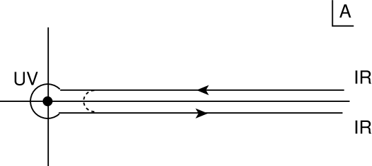
Figure 3: Contour of integration in the analytically-continued (regularized) version of $\Gamma(-s)$ for $s\in Z^{+}$. The quantity A denotes the (complex) world-sheet area. This is known in the literature as the Saalschutz contour, and has been used in conventional quantum field theory to relate dimensional regularization to the Bogoliubov-Parasiuk-Hepp-Zimmermann renormalization method. Upon the interpretation of the Liouville field with target time, this curve resembles closed-time-paths in non-equilibrium field theories.

We commence our analysis by considering the correlation functions among vertex operators in a generic Liouville theory, viewing the Liouville field as a local renormalization-group scale on the world sheet [4]. Standard computations[69] yield for an $N$-point correlation function among world-sheet integrated vertex operators $V_{i}\equiv\int d^{2}zV_{i}(z,{\bar{z}})$ :

$$A_{N}\equiv<V_{i_{1}}\dots V_{i_{N}}>_{\mu}=\Gamma(-s)\mu^{s}<(\int d^{2}z\sqrt{{\hat{\gamma}}}e^{\alpha\phi})^{s}{\tilde{V}}_{i_{1}}\dots\tilde{V}_{i_{N}}>_{\mu=0}$$ (3.92)

where the tilde denotes removal of the Liouville field $\phi$ zero mode, which has been path-integrated out in (3.92). The world-sheet scale $\mu$ is associated with cosmological constant terms on the world sheet, which are characteristic of the Liouville theory. The quantity $s$ is the sum of the Liouville anomalous dimensions of the operators $V_{i}$

$$s=-\sum_{i=1}^{N}\frac{\alpha_{i}}{\alpha}-\frac{Q}{\alpha}\qquad;\qquad\alpha=-\frac{Q}{2}+\frac{1}{2}\sqrt{Q^{2}+8}$$ (3.93)

The $\Gamma$ function can be regularized[5, 4] (for negative-integer values of its argument) by analytic continuation to the complex-area plane using the the Saaschultz contour of Fig. 3. Incidentally, this yields the possibility of an increase of the running central charge due to the induced oscillations of the dynamical world sheet area (related to the Liouville zero mode). This is associated with an oscillatory solution for the Liouville central charge near the fixed point. On the other hand, the bounce interpretation of the infrared fixed points of the flow, given in refs. [5, 4], provides an alternative picture of the overall monotonic change at a global level in target space-time.

To see technically why the above formalism leads to a breakdown in the interpretation of the correlator $A_{N}$ as a target-space string amplitude, which in turn leads to the interpretation of the world-sheet partition function as a probability density rather than a wave-function in target space, one first expands the Liouville field in (normalized) eigenfunctions $\{\phi_{n}\}$ of the Laplacian $\Delta$ on the world sheet

$$\phi(z,{\bar{z}})=\sum_{n}c_{n}\phi_{n}=c_{0}\phi_{0}+\sum_{n\neq 0}\phi_{n}\qquad\phi_{0}\propto A^{-\frac{1}{2}}$$ (3.94)

with $A$ the world-sheet area, and

$$\Delta\phi_{n}=-\epsilon_{n}\phi_{n}\qquad n=0,1,2,\dots,\qquad\epsilon_{0}=0\qquad(\phi_{n},\phi_{m})=\delta_{nm}$$ (3.95)

The result for the correlation functions (without the Liouville zero mode) appearing on the right-hand-side of eq. (3.92) is, then

$${\tilde{A}}_{N}\propto \int \Pi_{n\neq 0}dc_{n}exp(-\frac{1}{8\pi}\sum_{n\neq 0}\epsilon_{n}c_{n}^{2}-\frac{Q}{8\pi}\sum_{n\neq 0}R_{n}c_{n}+$$

$$\sum_{n\neq 0}\alpha_{i}\phi_{n}(z_{i})c_{n})(\int d^{2}\xi\sqrt{{\hat{\gamma}}}e^{\alpha\sum_{n\neq 0}\phi_{n}c_{n}})^{s}$$ (3.96)

with $R_{n}=\int d^{2}\xi R^{(2)}(\xi)\phi_{n}$. We can compute (3.96) if we analytically continue [69] $s$ to a positive integer $s\rightarrow n\in{\bf Z}^{+}$. Denoting

$$f(x,y)\equiv\sum_{n,m~{}\neq 0}\frac{\phi_{n}(x)\phi_{m}(y)}{\epsilon_{n}}$$ (3.97)

one observes that, as a result of the lack of the zero mode,

$$\Delta f(x,y)=-4\pi\delta^{(2)}(x,y)-\frac{1}{A}$$ (3.98)

We may choose the gauge condition $\int d^{2}\xi\sqrt{{\hat{\gamma}}}{\tilde{\phi}}=0$. This determines the conformal properties of the function $f$ as well as its ‘renormalized’ local limit

$$f_{R}(x,x)=lim_{x\rightarrow y}(f(x,y)+{\rm ln}d^{2}(x,y))$$ (3.99)

where $d^{2}(x,y)$ is the geodesic distance on the world sheet. Integrating over $c_{n}$ one obtains

$${\tilde{A}}_{n+N}\propto exp[\frac{1}{2}\sum_{i,j}\alpha_{i}\alpha_{j}f(z_{i},z_{j})+$$

$$\frac{Q^{2}}{128\pi^{2}}\int\int R(x)R(y)f(x,y)-\sum_{i}\frac{Q}{8\pi}\alpha_{i}\int\sqrt{{\hat{\gamma}}}R(x)f(x,z_{i})]$$ (3.100)

We now consider infinitesimal Weyl shifts of the world-sheet metric, $\gamma(x,y)\rightarrow\gamma(x,y)(1-\sigma(x,y))$, with $x,y$ denoting world-sheet coordinates. Under these, the correlator $A_{N}$ transforms as follows [4]

$$\delta{\tilde{A}}_{N}\propto[\sum_{i}h_{i}\sigma(z_{i})+\frac{Q^{2}}{16\pi}\int d^{2}x\sqrt{{\hat{\gamma}}}{\hat{R}}\sigma(x)+$$ (3.101)

$$\frac{1}{{\hat{A}}}\{Qs\int d^{2}x\sqrt{{\hat{\gamma}}}\sigma(x)+(s)^{2}\int d^{2}x\sqrt{{\hat{\gamma}}}\sigma(x){\hat{f}}_{R}(x,x)+$$

$$Qs\int\int d^{2}xd^{2}y\sqrt{{\hat{\gamma}}}R(x)\sigma(y){\hat{\mathcal{G}}}(x,y)-s\sum_{i}\alpha_{i}\int d^{2}x\sqrt{{\hat{\gamma}}}\sigma(x){\hat{\mathcal{G}}}(x,z_{i})-$$

$$\frac{1}{2}s\sum_{i}\alpha_{i}{\hat{f}}_{R}(z_{i},z_{i})\int d^{2}x\sqrt{{\hat{\gamma}}}\sigma(x)-$$

$$\frac{Qs}{16\pi}\int\int d^{2}xd^{2}y\sqrt{{\hat{\gamma}(x)}{\hat{\gamma}}(y)}{\hat{R}}(x){\hat{f}}_{R}(x,x)\sigma(y)\}]{\tilde{A}}_{N}$$

where the hat notation denotes transformed quantities, and the function ${\mathcal{G}}$(x,y) is defined as

$${\mathcal{G}}(z,\omega)\equiv f(z,\omega)-\frac{1}{2}(f_{R}(z,z)+f_{R}(\omega,\omega))$$ (3.102)

and transforms simply under Weyl shifts [4]. We observe from (3.101) that if the sum of the anomalous dimensions $s\neq 0$ (‘off-shell’ effect of non-critical strings), then there are non-covariant terms in (3.101), inversely proportional to the finite-size world-sheet area $A$. Thus the generic correlation function $A_{N}$ does not have a well-defined limit as $A\rightarrow 0$.

In our approach to string time we identify [4] the target time as $t=\phi_{0}=-{\rm log}A$, where $\phi_{0}$ is the world-sheet zero mode of the Liouville field. The normalization follows from a consequence of the canonical form of the kinetic term for the Liouville field $\phi$ in the Liouville $\sigma$ model [70, 4]. The opposite flow of the target time, as compared to that of the Liouville mode, is, on the other hand, a consequence of the ‘bounce’ picture [5, 4] for Liouville flow of Fig. 3. In view of this, the above-mentioned induced time (world-sheet scale $A$-) dependence of the correlation functions $A_{N}$ implies the breakdown of their interpretation as well-defined $S$-matrix elements, whenever there is a departure from criticality $s\neq 0$.

In general, this is a feature of non-critical strings wherever the Liouville mode is viewed as a local renormalization-group scale of the world sheet [4]. In such a case, the central charge of the theory flows continuously with the world-sheet scale $A$, as a result of the Zamolodchikov $c$-theorem [71]. In contrast, the screening operators in conventional strings yield quantized values[70]. Due to the analytic continuation curve illustrated in Fig. 3, we observe that upon interpreting the Liouville field $\phi$ as time [4]: $t\propto{\rm log}A$, the contour of Fig. 3 represents evolution in both directions of time between fixed points of the renormalization group: ${\rm Infrared}~{}{\rm fixed}~{}{\rm point}\rightarrow{\rm Ultraviolet}~{}{\rm fixed}~{}{\rm point}\rightarrow{\rm Infrared}~{}{\rm fixed}~{}{\rm point}$.

When one integrates over the Saalschultz contour in fig. 3, the integration around the simple pole at $A=0$ yields an imaginary part [5, 4], associated with the instability of the Liouville vacuum. We note, on the other hand, that the integral around the dashed contour shown in Fig. 3, which does not encircle the pole at $A=0$, is well defined. This can be interpreted as a well-defined $/S$-matrix element, which is not, however, factorisable into a product of $S-$ and $S^{\dagger}-$matrix elements, due to the $t$ dependence acquired after the identification $t=-{\rm log}A$.

Note that this formalism is similar to the Closed-Time-Path (CTP) formalism used in non-equilibrium quantum field theories [72]. Such formalisms are characterized by a ‘doubling of degrees of freedom’ (c.f. the two directions of the time (Liouville scale) curve of figure 3, in each of which one can define a set of dynamical fields in target space). As we discussed above, this prompts one to identify the corresponding Liouville correlators $A_{N}$ with $/S$-matrix elements rather than $S$-matrix elements in target space. Such elements act on the density matrices $\rho={\rm Tr}_{{\mathcal{M}}}|\Psi><\Psi|$ rather than wave vectors $|\Psi>$ in target space of the string: $\rho_{out}=/S\rho_{in}$ (c.f. the analogy with the $S$-matrix, $|out>=S|in>$).

This in turn implies that the world-sheet partition function ${\tilde{\mathcal{Z}}}_{\chi,L}$ of a Liouville string at a given world-sheet genus $\chi$, which is connected to the generating functional of the Liouville correlators $A_{N}$, when defined over the closed Liouville (time) path (CTP) of figure 3, can be associated with the probability density (diagonal element of a density matrix) rather than the wavefunction in the space of couplings. Indeed, one has

$${\tilde{\mathcal{Z}}}_{\chi,L}[g^{I}]=\int_{CTP}d\phi_{0}{\mathcal{Z}}_{\chi,L}[\phi_{0},g^{I}]$$ (3.103)

where $\{g^{I}\}$ denotes the set of couplings of the (non-conformal) deformations, $\phi_{0}\sim{\rm ln}A$ is the Liouville zero mode, and $A$ is the world-sheet area (renormalization-group scale). If one naively interprets ${\mathcal{Z}}_{\chi,L}[\phi_{0},g^{I}]$ as a wavefunctional in moduli space $\{g^{I}\}$, $\Psi[\phi_{0},g^{I}]$, then, in view of the double contour of figure 3, over which ${\tilde{\mathcal{Z}}}_{\chi,L}$ is defined, one encounters at each slice of constant $\phi_{0}$ a product of $\Psi[\phi_{0},g^{I}]\Psi^{\dagger}[\phi_{0},g^{I}]$, the complex conjugate wavefunctional corresponding to the second branch of the contour of opposite sense to the branch defining $\Psi[\phi_{0},g^{I}]$. This is analogous to the doubling of degrees of freedom in conventional thermal field theories [72]. Such products represent clearly probability densities ${\mathcal{P}}[t,g^{I}]$ in moduli space of the non-critical strings upon the identification of the Liouville zero mode $\phi_{0}$ with the target time $t$ [4].

In the above spirit, one may then consider the (formal) summation over world-sheet topologies $\chi$, and identify the summed-up world-sheet partition function $\sum_{\chi}{\mathcal{Z}}_{\chi,L}[\phi_{0},g^{I}]$ with the associated probability density in moduli space. In the case of D-particles, discussed in this work, the moduli space coincides with the configuration space (collective) coordinates of the D-particle soliton, and hence the corresponding probability density is associated with the position of the D-particle in target space. We stress once again that the above conclusion is based on the crucial assumption of the definition of the Liouville-string world-sheet partition function over the closed-time-path of figure 3. As we demonstrate in the main text, the specific D–brane example provide us with highly non-trivial consistency checks of this approach.

We would like now to give an explicit demonstration of the above ideas for the specific (simplified) case of recoiling (Abelian) D-particles. We shall demonstrate below that, upon considering the non-critical $\sigma$-model of a recoiling D-particle at a fixed world-sheet (Liouville) scale $\phi_{0}={\rm ln}A$, and identifying the Liouville mode with the target time, the Euclideanized world-sheet partition function can describe a probability density in moduli (collective coordinate) space.

To this end, let us first consider the pertinent $\sigma$ model partition function for a D-particle, at tree level and in a Minkowskian world-sheet $\Sigma$ formalism:

$${\mathcal{Z}}_{\chi=0,L}=\int(DX^{i})~{}e^{-i\frac{1}{4\pi\alpha^{\prime}}\int_{\Sigma}\partial X^{i}{\overline{\partial}}X^{j}\eta_{ij}-i\frac{1}{2\pi\alpha^{\prime}}\int_{\partial\Sigma}\left(\epsilon g_{i}^{C}+g_{i}^{D}\frac{1}{\epsilon}\right)\partial_{n}X^{i}}$$ (3.104)

where $\epsilon^{-2}\sim{\rm ln}\Lambda^{2}={\rm ln}A$ (c.f. (3.118)), on account of the logarithmic algebra [52]. In our approach $\epsilon^{-2}$ is identified with the target time. This is why in (3.104) we have not path-integrated over $X^{0}$, but we consider an integral only over the spatial collective coordinates $X^{i},i=1,\dots 9$ of the D-particle. The combination of $\sigma$-model couplings $\epsilon g_{i}^{C}+g_{i}^{D}\frac{1}{\epsilon}$ may be identified with the generalized (Abelian) position $\epsilon Y^{i}$ of the recoiling D-particle (3.113). Notice that, since here we have already identified the time with the scale $\epsilon^{-2}>0$, the step function in the recoil deformations of the $\sigma$-model (3.114) acquires trivial meaning. We shall come back to a discussion on how one can incorporate a world-sheet dependence in the time coordinate later on.

Suppose now that, following the spirit of critical strings [44], one identifies the Minkowskian world-sheet partition function (3.104) with a wavefunctional $\Psi[Y^{i},\phi_{0}=t]$. The probability density in $Y^{i}$ space, ${\mathcal{P}}[Y^{i},t]=\Psi[Y^{i},t]\Psi^{*}[Y^{i},t]$, reads in this case:

$$\left|{\mathcal{Z}}_{\chi=0,L}[Y^{i},t]\right|^{2}=$$

$$\int DX^{i}\int DX^{\prime j}e^{-i\frac{1}{4\pi\alpha^{\prime}}\int_{\Sigma}\partial X^{i}{\overline{\partial}}X^{j}\eta_{ij}+i\frac{1}{4\pi\alpha^{\prime}}\int_{\Sigma}\partial X^{\prime i}{\overline{\partial}}X^{\prime j}\eta_{ij}-i\frac{1}{2\pi\alpha^{\prime}}\int_{\partial\Sigma}\epsilon Y_{i}(t)\partial_{n}(X^{i}-X^{\prime i})}=$$

$$\left(\int DX_{-}^{i}e^{i\frac{1}{4\pi\alpha^{\prime}}\int_{\Sigma}\partial X_{-}^{i}{\overline{\partial}}X_{-}^{j}\eta_{ij}-i\frac{1}{2\pi\alpha^{\prime}}\int_{\partial\Sigma}Y_{i}(t)\partial_{n}X_{-}^{i}}\right)\otimes(\left(\int DX_{+}^{i}e^{-i\frac{1}{4\pi\alpha^{\prime}}\int_{\Sigma}\partial X_{+}^{i}{\overline{\partial}}X_{+}^{j}\eta_{ij}}\right)~{},$$

(3.105)

where $X_{\pm}^{i}=X^{i}\pm X^{\prime i}$. Upon passing to a Euclidean world-sheet formalism, and taking into account that the $Y_{i}$ independent factor can be absorbed in appropriate normalization of the $\sigma$-model correlators, one then proves our statement that $\sigma$-model partition functions in non-critical strings can be identified with moduli space probability densities.

Notice that similar conclusions can be reached even in the case where the time $X^{0}$ is included in the analysis as a full fledged world-sheet field and is only eventually identified with the Liouville mode. In such a case, by considering the probability density as above, one is confronted with path integration over $X_{\pm}^{0}=X_{0}\pm X^{\prime 0}$ $\sigma$-model fields, which also appear in the arguments of the step function operators $\Theta_{\epsilon}(X_{\pm}^{0})$ in the recoil deformations (c.f. below, (3.114)), that are non trivial in this case. However, upon Liouville dressing and the requirement that the Liouville mode be identified with the target time, one is forced to restrict oneself on the hypersurface $X_{-}=0$ in the corresponding path integral $\int DX_{+}^{0}DX_{-}^{0}(\dots)$. As a consequence, one is then left with a world-sheet partition function integrated only over the Liouville mode $X_{+}=2\phi$ (c.f. ${\tilde{\mathcal{Z}}}$ in (3.103)), and hence the identification of a Liouville string partition function with a probability density in moduli space is still valid, upon passing onto a Euclideanized world-sheet formalism. It can also be seen, in a straightforward manner, that summing upon higher world-sheet topologies, as in [2], will not change this conclusion.

Notice that if one interprets the topological expansion of the worldsheet partition function as the probability density for the non-critical string configuration $\{g^{I}\}$, then the simple argument leading to eq. (3.80) is not valid here. In such a situation the action in eq. (3.82), which refers to the string moduli space, is not the same as the effective target space action ${\mathcal{F}}[\{g^{I}\}]$, but rather something different, corresponding to the phase of the wavefunctional $\Psi(\{g^{I}\},t)$ whose probability density (3.91) corresponds to the genera summed worldsheet partition function. This is not necessarily a bad feature, as we shall see, although in most treatments the target space effective action ${\mathcal{F}}[\{g^{I}\}]$ is identified with the moduli space action upon identification of the Liouville zero mode (i.e. the local worldsheet renormalization group scale) with target time. For this, we observe that the statistical interpretation of the resummed worldsheet partition function is compatible with the interpretation in [2] of the Gaussian wormhole parameter distribution function in eq. (3.90) as being responsible for the quantum uncertainties of D-branes. This follows trivially from the fact that

$$\left|\Psi(\{g^{I}\},t)\right|^{2}={\,\rm e}\,^{-2{\mathcal{F}}(\{g^{I}\},t)}$$ (3.106)

Then, any correlation function may be written as

$$\left\langle V_{I_{1}}\cdots V_{I_{n}}\right\rangle=\int\limits_{{\hbox{\mybbs M}}(\{g^{I}\})}Dg^{I}~{}\left|\Psi(\{g^{I}\},t)\right|^{2}\,V_{I_{1}}\cdots V_{I_{n}}=$$

$$\int\limits_{{\hbox{\mybbs M}}(\{g^{I}\})}Dg^{I}~{}\int\limits_{{\hbox{\mybbs M}}(\{g^{I}\})}D\alpha^{I}~{}{\,\rm e}\,^{-\frac{1}{2\Gamma^{2}}\alpha^{I}G_{IJ}\alpha^{J}}\,\int Dx~{}{\,\rm e}\,^{-S_{\sigma}^{(0)}[x;\{g^{I}+\alpha^{I}\}]}\,V_{I_{1}}\cdots V_{I_{n}}$$ (3.107)

which using eq. (3.106) gives the connection between the two probability distributions.

3.3 Matrix D-brane Dynamics

In this section we shall briefly review the worldsheet description of [2] for matrix D0-brane dynamics. The partition function is given by [41]

$${\mathcal{Z}}[A_{0},Y] = \int D\mu(x,\bar{\xi},\xi)~{}\exp\left(-\frac{1}{4\pi\alpha^{\prime}}\int\limits_{\Sigma}d^{2}z~{}\eta_{\mu\nu}\,\partial x^{\mu}\,\bar{\partial}x^{\nu}+\frac{1}{2\pi\alpha^{\prime}}\oint\limits_{\partial\Sigma}d\tau~{}x_{i}(\tau)\,\partial_{\sigma}x^{i}(\tau)\right)$$ (3.108)

$$\times\,{\mathcal{W}}[x,\bar{\xi},\xi]$$

where

$${\mathcal{W}}[x,\bar{\xi},\xi]=\exp ig_{s}\oint\limits_{\partial\Sigma}d\tau~{}\left(\bar{\xi}_{a}(\tau)A_{0}^{ab}\xi_{b}(\tau)\,\partial_{\tau}x^{0}(\tau)+\frac{i}{2\pi\alpha^{\prime}}\,\bar{\xi}_{a}(\tau)Y_{i}^{ab}(x^{0})\xi_{b}(\tau)\,\partial_{\sigma}x^{i}(\tau)\right)$$ (3.109)

is the deformation action of the free $\sigma$-model in (3.108). Here the indices $\mu=0,1,\dots,9$ and $i=1,\dots,9$ label spacetime and spatial directions of the target space, which we assume has a flat metric $\eta_{\mu\nu}$. The functional integration measure in (3.108) is given by

$$D\mu(x,\bar{\xi},\xi)=Dx^{\mu}~{}D\bar{\xi}~{}D\xi~{}\exp\left[-\sum_{a=1}^{N}\left(\oint\limits_{\partial\Sigma}d\tau~{}\bar{\xi}_{a}(\tau)\,\partial_{\tau}\xi_{a}(\tau)+\bar{\xi}_{a}(0)\xi_{a}(0)\right)\right]\times$$

$$\sum_{a=1}^{N}\bar{\xi}_{a}(0)\xi_{a}(1)$$ (3.110)

The complex auxiliary fields $\bar{\xi}_{a}(\tau)$ and $\xi_{a}(\tau)$, $a=1,\dots,N$, transform in the fundamental representation of the brane gauge group, and they live on the boundary of the worldsheet $\Sigma$ which at tree-level is a disc whose boundary is a circle $\partial\Sigma$ with periodic longitudinal coordinate $\tau\in[0,1]$ and normal coordinate $\sigma\in{\hbox{\mybb R}}$. They have the propagator $\langle\bar{\xi}_{a}(\tau)\xi_{b}(\tau^{\prime})\rangle=\delta_{ab}\,\Theta(\tau^{\prime}-\tau)$, where $\Theta$ denotes the usual step function. The integration over the auxiliary fields with the measure (3.110) therefore turns (3.109) into a path-ordered exponential functional of the fields $x$ which is the $T$-dual of the usual Wilson loop operator for the ten-dimensional gauge field $(A^{0},-\frac{1}{2\pi\alpha^{\prime}}Y^{i})$ dimensionally reduced to the D-particle worldlines. In this picture, $A^{0}$ is thought of as a gauge field living on the brane worldline, while $Y_{i}^{aa}$, $a=1,\dots,N$, are the transverse coordinates of the $N$ D-particles and $Y_{i}^{ab}$, $a\neq b$, of the short open string excitations connecting them. We shall subtract out the center of mass motion of the assembly of $N$ D-branes and assume that $Y_{i}\in su(N)$. We shall also use $SU(N)$-invariance of the theory (3.108) to select the temporal gauge $A^{0}=0$.

The action in (3.108) may be formally identified with the deformed conformal field theory (3.74) by taking the couplings $g^{I}\sim Y_{i}^{ab}$ and introducing the one-parameter family of bare matrix-valued vertex operators

$$V_{ab}^{i}(x;\tau)=\frac{g_{s}}{2\pi\alpha^{\prime}}\,\partial_{\sigma}x^{i}(\tau)\,\bar{\xi}_{a}(\tau)\xi_{b}(\tau)$$ (3.111)

This means that there is a one-parameter family of Dirichlet boundary conditions for the fundamental string fields $x^{i}$ on $\partial\Sigma$, labeled by $\tau\in[0,1]$ and the configuration fields

$$y_{i}(x^{0};\tau)=\bar{\xi}_{a}(\tau)\,Y_{i}^{ab}(x^{0}(\tau))\,\xi_{b}(\tau)$$ (3.112)

Instead of being forced to sit on a unique hypersurface as in the case of a single D-brane, in the non-abelian case there is an infinite set of hypersurfaces on which the string endpoints are situated. In this sense the coordinates (3.112) may be thought of as an “abelianization” of the non-abelian D-particle coordinate fields $Y_{i}^{ab}$.

To describe the non-relativistic dynamics of heavy D-particles, the natural choice is to take the couplings to correspond to the Galilean boosted configurations $Y_{i}^{ab}(x^{0})=Y_{i}^{ab}+U_{i}^{ab}x^{0}$, where $U_{i}$ is the non-relativistic velocity matrix. However, logarithmic modular divergences appear in matter field amplitudes at higher genera when the string propagator $L_{0}$ is computed with Dirichlet boundary conditions. These modular divergences are canceled by adding logarithmic recoil operators [2, 52] to the matrix $\sigma$-model action in (3.108). From a physical point of view, if one is to use low-energy probes to observe short-distance spacetime structure, such as a generalized Heisenberg microscope, then one needs to consider the scattering of string matter off the assembly of D-particles. For the Galilean-boosted multiple D-particle system, the recoil is described by taking the deformation of the $\sigma$-model action in (3.108) to be of the form [2]

$$Y_{i}^{ab}(x^{0})=\sqrt{\alpha^{\prime}}\,Y_{i}^{ab}C_{\epsilon}(x^{0})+U_{i}^{ab}D_{\epsilon}(x^{0})=\left(\sqrt{\alpha^{\prime}}\,\epsilon Y_{i}^{ab}+U_{i}^{ab}x^{0}\right)\Theta_{\epsilon}(x^{0})$$ (3.113)

where

$$C_{\epsilon}(x^{0})=\epsilon\,\Theta_{\epsilon}(x^{0})~{}~{}~{}~{}~{}~{},~{}~{}~{}~{}~{}~{}D_{\epsilon}(x^{0})=x^{0}\,\Theta_{\epsilon}(x^{0})$$ (3.114)

and

$$\Theta_{\epsilon}(x^{0})=\frac{1}{2\pi i}\int\limits_{-\infty}^{+\infty}\frac{dq}{q-i\epsilon}~{}{\,\rm e}\,^{iqx^{0}}$$ (3.115)

is the regulated step function whose $\epsilon\to 0^{+}$ limit is the usual step function. The operators (3.114) have non-vanishing matrix elements between different string states and therefore describe the appropriate change of quantum state of the D-brane background. They can be thought of as describing the recoil of the assembly of D-particles in an impulse approximation, in which it starts moving as a whole only at time $x^{0}=0$. The collection of constant matrices $\{Y^{i}_{ab},U^{j}_{cd}\}$ now form the set of coupling constants $\{g^{I}\}$ for the worldsheet $\sigma$-model (3.108).

As discussed previously, the recoil operators (3.114) possess a very important property. They lead to a deformation of the free $\sigma$-model action in (3.108) which is not conformally-invariant, but rather defines a logarithmic conformal field theory [6, 7]. Such a quantum field theory contains logarithmic scaling violations in its correlation functions on the worldsheet, which can be seen in the present case by computing the pair correlators of the fields (3.114) [52]

$$\Bigl{\langle}C_{\epsilon}(z)\,C_{\epsilon}(0)\Bigr{\rangle} = 0$$

$$\Bigl{\langle}C_{\epsilon}(z)\,D_{\epsilon}(0)\Bigr{\rangle} = \frac{b}{z^{h_{\epsilon}}}$$

$$\Bigl{\langle}D_{\epsilon}(z)\,D_{\epsilon}(0)\Bigr{\rangle} = \frac{b\,\alpha^{\prime}}{z^{h_{\epsilon}}}\,\log z$$ (3.116)

where

$$h_{\epsilon}=-\frac{|\epsilon|^{2}\,\alpha^{\prime}}{2}$$ (3.117)

is the conformal dimension of the recoil operators. The constant $b$ is fixed by the leading logarithmic divergence of the conformal blocks of the theory. Note that (3.117) vanishes as $\epsilon\to 0$, so that the logarithmic worldsheet divergences in (3.116) cancel the modular annulus divergences mentioned above. An essential ingredient for this cancellation is the identification [52]

$$\frac{1}{\epsilon^{2}}=-2\alpha^{\prime}\log\Lambda$$ (3.118)

which relates the target space regularization parameter $\epsilon$ to the worldsheet ultraviolet cutoff scale $\Lambda$.

Logarithmic conformal field theories are characterized by the fact that their Virasoro generator $L_{0}$ is not diagonalizable, but rather admits a Jordan cell structure. Here the operators (3.114) form the basis of a $2\times 2$ Jordan block and they appear in the spectrum of the two-dimensional quantum field theory as a consequence of the zero modes that arise from the breaking of the target space translation symmetry by the topological defects. The mixing between $C$ and $D$ under a conformal transformation of the worldsheet can be seen explicitly by considering a scale transformation

$$\Lambda\to\Lambda^{\prime}=\Lambda\,{\,\rm e}\,^{-t/\sqrt{\alpha^{\prime}}}$$ (3.119)

Using (3.118) it follows that the operators (3.114) are changed according to $D_{\epsilon}^{\prime}=D_{\epsilon}+t\sqrt{\alpha^{\prime}}C_{\epsilon}$ and $C_{\epsilon}^{\prime}=C_{\epsilon}$. Thus in order to maintain scale-invariance of the theory (3.108) the coupling constants must transform under (3.119) as [52, 53] $Y^{\prime i}=Y^{i}+U^{i}t$ and $U^{\prime i}=U^{i}$, which are just the Galilean transformation laws for the positions $Y^{i}$ and velocities $U^{i}$. Thus a scale transformation of the worldsheet is equivalent to a Galilean transformation of the moduli space of $\sigma$-model couplings, with the parameter $\epsilon^{-2}$ identified with the time evolution parameter $t=-\sqrt{\alpha^{\prime}}\log\Lambda$. The corresponding $\beta$-functions for the worldsheet renormalization group flow are

$$\beta_{Y_{i}} \equiv \frac{dY_{i}}{dt}=h_{\epsilon}\,Y_{i}+\sqrt{\alpha^{\prime}}\,U_{i}$$

$$\beta_{U_{i}} \equiv \frac{dU_{i}}{dt}=h_{\epsilon}\,U_{i}$$ (3.120)

and they generate the Galilean group $G(9)^{N^{2}}$ in nine-dimensions.

The associated Zamolodchikov metric

$$G_{ab;cd}^{ij}=2N\Lambda^{2}\left\langle V_{ab}^{i}(x;0)\,V_{cd}^{j}(x;0)\right\rangle$$ (3.121)

can be evaluated to leading orders in $\sigma$-model perturbation theory using the logarithmic conformal algebra (3.116) and the propagator of the auxiliary fields to give [2]

$$G_{ab;cd}^{ij} = \frac{4\bar{g}_{s}^{2}}{\alpha^{\prime}}\left[\eta^{ij}\,I_{N}\otimes I_{N}+\frac{\bar{g}_{s}^{2}}{36}\left\{I_{N}\otimes\left(\bar{U}^{i}\bar{U}^{j}+\bar{U}^{j}\bar{U}^{i}\right)\right.\right.$$ (3.122)

$$\biggl{.}\left.+\,\bar{U}^{i}\otimes\bar{U}^{j}+\bar{U}^{j}\otimes\bar{U}^{i}+\left(\bar{U}^{i}\bar{U}^{j}+\bar{U}^{j}\bar{U}^{i}\right)\otimes I_{N}\right\}\biggr{]}_{db;ca}+$$

$${\mathcal{O}}\left(\bar{g}_{s}^{6}\right)$$

where $I_{N}$ is the identity operator of $SU(N)$ and we have introduced the renormalized coupling constants

$$\bar{g}_{s}=g_{s}/\sqrt{\alpha^{\prime}}\epsilon~{}~{}~{}~{}~{}~{},~{}~{}~{}~{}~{}~{}\bar{U}^{i}=U^{i}/\sqrt{\alpha^{\prime}}\epsilon$$ (3.123)

From the renormalization group equations (3.120) it follows that the renormalized velocity operator in target space is truly marginal,

$$\frac{d\bar{U}^{i}}{dt}=0$$ (3.124)

which ensures uniform motion of the D-branes. It can also be shown that the renormalized string coupling $\bar{g}_{s}$ is time-independent [2]. If we further define the position renormalization

$$\bar{Y}^{i}=Y^{i}/\sqrt{\alpha^{\prime}}\epsilon$$ (3.125)

then the $\beta$-function equations (3.120) coincide with the Galilean equations of motion of the D-particles, i.e.

$$\frac{d\bar{Y}^{i}}{dt}=\bar{U}^{i}$$ (3.126)

Note that the Zamolodchikov metric (3.122) is a complicated function of the D-brane dynamical parameters, and as such it represents the appropriate effective target space geometry of the D-particles. The moduli space Lagrangian (3.89) is then readily seen to coincide with the expansion to ${\mathcal{O}}(\bar{g}_{s}^{4})$ of the symmetrized form of the non-abelian Born-Infeld action for the D-brane dynamics [39],

$${\mathcal{L}}_{\rm NBI}=\frac{1}{\sqrt{2\pi\alpha^{\prime}}\bar{g}_{s}}\,\>{\rm tr}\,~{}{\rm Sym}\,\sqrt{\det_{\mu,\nu}\left[\eta_{\mu\nu}\,I_{N}+2\pi\alpha^{\prime}\bar{g}_{s}^{2}\,F_{\mu\nu}\right]}$$ (3.127)

where tr denotes the trace in the fundamental representation of $SU(N)$,

$${\rm Sym}(M_{1},\dots,M_{n})=\frac{1}{n!}\sum_{\pi\in S_{n}}M_{\pi_{1}}\cdots M_{\pi_{n}}$$ (3.128)

is the symmetrized matrix product and the components of the dimensionally reduced field strength tensor are given by

$$F_{0i}=\frac{1}{2\pi\alpha^{\prime}}\,\frac{d{\bar{Y}}_{i}}{dt}~{}~{}~{}~{}~{}~{},~{}~{}~{}~{}~{}~{}F_{ij}=\frac{\bar{g}_{s}}{(2\pi\alpha^{\prime})^{2}}\left[\bar{Y}_{i}\,,\,\bar{Y}_{j}\right]$$ (3.129)

3.4 Evolution Equation for the Probability Distribution

In this section we will derive the temporal evolution equation for the probability density ${\mathcal{P}}(\{g^{I}\},t)$ following the identification of time with a worldsheet renormalization group scale (i.e. the Liouville zero mode). The basic identity is the Wilson-Polchinski equation for the case of the worldsheet action (3.74) which reads [44]

$$0 = \frac{\partial{\mathcal{Z}}}{\partial\log\Lambda}$$ (3.130)

$$= \int Dx^{\mu}~{}{\,\rm e}\,^{-S_{\sigma}[x;\{g^{I}\}]}\,\left\{\frac{\partial S_{\rm int}}{\partial\log\Lambda}\right.$$

$$\left.-\,\int\limits_{\Sigma}d^{2}z~{}\int\limits_{\Sigma}d^{2}w~{}\left(\frac{\partial}{\partial\log\Lambda}G(z-w)\right)\left[\frac{\delta^{2}S_{\rm int}}{\delta x^{\mu}(z)\delta x_{\mu}(w)}+\frac{\delta S_{\rm int}}{\delta x^{\mu}(z)}\frac{\delta S_{\rm int}}{\delta x_{\mu}(w)}\right]\right\}$$

and it is the requirement of conformal invariance of the quantum string theory. Here $S_{\rm int}=S_{\sigma}-S_{*}$, $\mathcal{Z}$ is the partition function of the $\sigma$-model, and

$$G(z-w)=\left\langle\,\mbox{$\circ\atop\circ$}\,x^{\mu}(z)x_{\mu}(w)\,\mbox{$\circ\atop\circ$}\,\right\rangle_{*}$$ (3.131)

is the two-point function computed with respect to the conformal field theory action $S_{*}[x]$. The basic assumption in arriving at eq. (3.130) is that the ultra-violet cutoff $\Lambda$ on the string worldsheet appears explicitly only in the propagator $G(z-w)$, as can always be arranged by an appropriate regularization [44].

Henceforth we shall concentrate on the specific case of interest of a system of $N$ interacting D-particles. Then, upon summing up over pinched genera, there are extra logarithmic divergences in the Green’s function (3.131) coming from pinched annulus diagrams, which may be removed by the introduction of logarithmic recoil operators, as explained in the previous section. Using primes to denote the result of resumming the topological expansion over pinched genera, we then have that

$$\frac{\partial}{\partial\log\Lambda}G(z-w)^{\prime}=\frac{\partial}{\partial\log\Lambda}{\sum_{\rm genera}}^{\prime}\left\langle\,\mbox{$\circ\atop\circ$}\,x^{\mu}(z)x_{\mu}(w)\,\mbox{$\circ\atop\circ$}\,\right\rangle=\frac{\partial}{\partial\log\Lambda}\left\langle\,\mbox{$\circ\atop\circ$}\,x^{\mu}(z)x_{\mu}(w)\,\mbox{$\circ\atop\circ$}\,\right\rangle_{\rm int}$$ (3.132)

where the correlator $\langle\cdot\rangle_{\rm int}$ includes the disc and recoil interaction contributions. Subtracting the disc $\Lambda$-dependence in normal ordering, the remaining dependence on the worldsheet cutoff comes from the two-point functions of the logarithmic recoil operators, giving terms of the form

$$\frac{\partial}{\partial\log\Lambda}\left\langle\,\mbox{$\circ\atop\circ$}\,x^{\mu}(z)x_{\mu}(w)\,\mbox{$\circ\atop\circ$}\,\Bigl{(}a_{CC}C_{\epsilon}(z)C_{\epsilon}(w)+a_{CD}C_{\epsilon}(z)D_{\epsilon}(w)+a_{DD}D_{\epsilon}(z)D_{\epsilon}(w)\Bigr{)}\right\rangle_{*}$$ (3.133)

The leading divergence comes from the correlation function $\langle D_{\epsilon}(z)D_{\epsilon}(w)\rangle_{*}\sim\log\Lambda$, which follows upon the identification (3.118). Thus we may write

$$\frac{\partial}{\partial\log\Lambda}G(z-w)\simeq c_{G}\,(\alpha^{\prime})^{2}\log|z-w|\,\sum_{i=1}^{9}\,\sum_{a,b=1}^{N}|U_{ab}^{i}|^{2}$$ (3.134)

where $c_{G}>0$ is a numerical coefficient whose precise value is not important, and we have used the fact that $U^{i}\in su(N)$.

Next, we observe that in the case of D-particles the second term in eq. (3.130) becomes

$$\int D\mu(x,\bar{\xi},\xi)~{}{\,\rm e}\,^{-S_{\sigma}}\,\oint\limits_{\partial\Sigma}d\tau~{}\oint\limits_{\partial\Sigma}d\tau^{\prime}~{}(\alpha^{\prime})^{2}c_{G}\sum_{i=1}^{9}\sum_{a,b=1}^{N}|U_{ab}^{i}|^{2}\,\log[2-2\cos(\tau-\tau^{\prime})]$$

$$~{}~{}~{}~{}~{}~{}\times\,\left[\frac{\delta^{2}S_{\rm int}}{\delta x^{\mu}(\tau)\delta x_{\mu}(\tau^{\prime})}+\frac{\delta S_{\rm int}}{\delta x^{\mu}(\tau)}\frac{\delta S_{\rm int}}{\delta x_{\mu}(\tau^{\prime})}\right]$$ (3.135)

where the interaction Lagrangian is given by

$$S_{\rm int}=\frac{g_{s}}{2\pi\alpha^{\prime}}\oint\limits_{\partial\Sigma}d\tau~{}\partial_{\sigma}x^{i}(\tau)\,\bar{\xi}_{a}(\tau)\,Y_{i}^{ab}(x^{0})\,\xi_{b}(\tau)$$ (3.136)

In the case of a system of recoiling D0-branes, the $\sigma$-model couplings in eq. (3.136) are given by (3.113) with the abelianized couplings (3.112) of $Y_{i}^{ab}$ viewed as the boundary values for the open string embedding fields $x^{i}(\tau)$ on the D-brane. This means that the fields $x^{i}(\tau)$ are simply identified with $\bar{\xi}_{a}(\tau)Y_{i}^{ab}\xi_{b}(\tau)$. All the non-trivial dependence comes from the $x^{0}$ field which obeys Neumann boundary conditions and is not constant on the boundary of $\Sigma$. Then we may write

$$\frac{\delta^{2}S_{\rm int}}{\delta x^{\mu}(\tau)\delta x_{\mu}(\tau^{\prime})}+\frac{\delta S_{\rm int}}{\delta x^{\mu}(\tau)}\frac{\delta S_{\rm int}}{\delta x_{\mu}(\tau^{\prime})}$$

$$~{}~{}~{}~{}=\nabla_{y_{i}}^{2}S_{\rm int}+\left(\nabla_{y_{i}}S_{\rm int}\right)^{2}+\left(\frac{g_{s}}{2\pi\alpha^{\prime}}\right)^{2}\,U_{i}^{ab}U_{j}^{cd}\bar{\xi}_{a}(\tau)\xi_{b}(\tau)\bar{\xi}_{c}(\tau^{\prime})\xi_{d}(\tau^{\prime})$$

$$~{}~{}~{}~{}~{}~{}\times\,\partial_{\sigma}x^{i}(\tau)\partial_{\sigma}x^{j}(\tau^{\prime})\Theta_{\epsilon}(x^{0}(\tau))\Theta_{\epsilon}(x^{0}(\tau^{\prime}))$$ (3.137)

where $y_{i}$ denotes the constant abelianized zero modes of $x^{i}(\tau)$ on $\partial\Sigma$. Here we have used the fact that terms of the form $x^{0}\delta(x^{0})$ and $\Theta(x^{0})\delta(x^{0})$ vanish with the regularization (3.115) [2]. The terms involving $\partial_{\sigma}x^{i}(\tau)\partial_{\sigma}x^{j}(\tau^{\prime})$ will average out to yield terms of the form

$$|U_{ab}^{i}|^{2}\left\langle\Theta_{\epsilon}(x^{0}(\tau))\Theta_{\epsilon}(x^{0}(\tau^{\prime}))\right\rangle_{*}=\alpha^{\prime}|\bar{U}_{ab}^{i}|^{2}\left\langle C_{\epsilon}(\tau)C_{\epsilon}(\tau^{\prime})\right\rangle_{*}\sim{\mathcal{O}}(\epsilon^{2})$$ (3.138)

where we have used the logarithmic conformal algebra. At leading orders, these terms vanish, but we shall see the importance of such sub-leading terms later on.

Using the Dirichlet correlator

$$\left\langle\partial_{\sigma}x^{i}(\tau)\partial_{\sigma}x_{i}(\tau^{\prime})\right\rangle_{*}=-\frac{36\pi^{2}\alpha^{\prime}}{1-\cos(\tau-\tau^{\prime})}$$ (3.139)

we find that the boundary integrations in eq. (3.135) are of the form [2]

$$\oint\limits_{\partial\Sigma}d\tau~{}\oint\limits_{\partial\Sigma}d\tau^{\prime}~{}\frac{\log[2-2\cos(\tau-\tau^{\prime})]}{1-\cos(\tau-\tau^{\prime})}\sim\log\Lambda$$ (3.140)

which has the effect of renormalizing the velocity matrix $U_{ab}^{i}\to\bar{U}_{ab}^{i}$. Thus, ignoring the ${\mathcal{O}}(\epsilon^{2})$ terms for the moment, we find that the remaining terms in the Wilson-Polchinski renormalization group equation (3.130) yield a diffusion term for the probability density:

$$\partial_{t}{\mathcal{P}}[Y,U;t]=c_{G}\sqrt{\alpha^{\prime}}\sum_{j=1}^{9}\sum_{a,b=1}^{N}|\bar{U}_{ab}^{j}|^{2}\,\nabla_{y_{i}}^{2}{\mathcal{P}}[Y,U;t]+{\mathcal{O}}(\epsilon^{2})$$ (3.141)

This equation is of the Fokker-Planck type, with diffusion coefficient

$${\mathcal{D}}=c_{G}\sqrt{\alpha^{\prime}}\sum_{i=1}^{9}\sum_{a,b=1}^{N}|\bar{U}_{ab}^{i}|^{2}$$ (3.142)

coming from the quantum recoil of the assembly of D-particles. The diffusion disappears when there is no recoil. Note that (3.142) naturally incorporates the short-distance quantum gravitational smearings for the open string interactions (compare with eq. (3.65)), and it arises as an abelianized velocity for the constant auxiliary field configuration $\bar{\xi}_{a}(\tau)=\xi_{a}(\tau)=1~{}~{}\forall a=1,\dots,N$.

The evolution equation (3.141) should be thought of as a modification of the usual continuity equation for the probability density. Indeed, as we will now show, the ${\mathcal{O}}(\epsilon^{2})$ terms in eq. (3.141) coming from (3.138) are of the form $-\nabla_{y_{i}}{\mathcal{J}}_{i}$, where

$${\mathcal{J}}_{i}=\frac{\hbar_{\hbox{\mybbs M}}}{2im}\left(\Psi^{\dagger}\,\nabla_{y_{i}}\Psi-\Psi\,\nabla_{y_{i}}\Psi^{\dagger}\right)$$ (3.143)

is the probability current density. Here

$$m=\frac{1}{\sqrt{\alpha^{\prime}}\bar{g}_{s}}~{}~{}~{}~{}~{}~{},~{}~{}~{}~{}~{}~{}\hbar_{\hbox{\mybbs M}}=4\bar{g}_{s}$$ (3.144)

are, respectively, the BPS mass of the D-particles and the moduli space “Planck constant”. 

For this, we note first of all that such terms should generically come in the form

$$-\nabla_{y_{i}}{\mathcal{J}}_{i}=-\frac{\hbar_{\hbox{\mybbs M}}}{m}\left(\nabla_{y_{i}}^{2}\,{\rm arg}\,\Psi\right){\mathcal{P}}-\frac{\hbar_{\hbox{\mybbs M}}}{m}\left(\nabla_{y_{i}}\,{\rm arg}\,\Psi\right)\nabla_{y_{i}}{\mathcal{P}}$$ (3.145)

The second term in eq. (3.145), upon identification of the probability density $\mathcal{P}$ with the genera resummed partition function on the string worldsheet, is proportional to the worldsheet renormalization group $\beta$-function, given the gradient flow property (3.77) of the string effective action [50], so that

$$\nabla_{y_{i}}{\mathcal{P}}=-2{\mathcal{P}}\,G_{ij}\beta^{j}$$ (3.146)

which is to be understood in terms of abelianized quantities. In the present case the renormalization group equations are given by (3.124) and (3.126) and, since the couplings $\bar{U}_{i}^{ab}$ are truly marginal, we are left in (3.146) with only a Zamolodchikov metric contribution $G_{CC}=2N\Lambda^{4}\langle C_{\epsilon}(\tau)C_{\epsilon}(\tau)\rangle_{*}$ (Note that here one should use suitably normalized correlators $\langle\cdot\rangle_{*}$ which yield the behavior (3.146)). From the logarithmic conformal algebra it therefore follows that a term with the structure of the second piece in eq. (3.145) is hidden in the contributions (3.138) which were dropped as being subleading in $\epsilon$. Furthermore, from (3.122), (3.145), (3.134), (3.137) and (3.138) it follows that to leading orders

$$\nabla_{y_{i}}\,{\rm arg}\,\Psi=-\frac{c_{G}}{\sqrt{\alpha^{\prime}}\bar{u}_{i}}\left(\sum_{j=1}^{9}\sum_{a,b=1}^{N}|\bar{U}_{ab}^{j}|^{2}\right)^{2}$$ (3.147)

where $\bar{u}_{i}=d\bar{y}_{i}/dt$ is the worldsheet zero mode of the abelianized, renormalized velocity operator. It then follows that to leading orders we have $\nabla_{y_{i}}^{2}\,{\rm arg}\,\Psi=0$.

Thus, keeping the subleading terms in the target space regularization parameter $\epsilon$ leads to the complete Fokker-Planck equation for the probability density ${\mathcal{P}}=\Psi^{\dagger}\Psi$:

$$\partial_{t}{\mathcal{P}}[Y,U;t]=-\nabla_{y_{i}}{\mathcal{J}}_{i}[Y,U;t]+{\mathcal{D}}\,\nabla_{y_{i}}^{2}{\mathcal{P}}[Y,U;t]$$ (3.148)

where ${\mathcal{J}}_{i}$ is the probability current density (3.143), with $\Psi$ the wavefunctional for the system of D-branes:

$$\Psi[Y,U;t]=\prod_{i=1}^{9}\exp\left[-\frac{ic_{G}}{\sqrt{\alpha^{\prime}}}\frac{y_{i}}{\bar{u}_{i}}\left(\sum_{j=1}^{9}\>{\rm tr}\,\,|\bar{U}^{j}|^{2}\right)^{2}\right]\,\Bigl{|}\Psi[Y,U;t]\Bigr{|}$$ (3.149)

Such quantum diffusion is characteristic of all Liouville string theories [45, 47, 54]. The resulting quantum dynamics, including the quantum diffusion which arises from the D-brane recoil, is described by the Schrödinger wave equation which corresponds to this Fokker-Planck equation. This equation is analyzed in detail in the next section.

3.5 Non-linear Schrödinger Wave Equations

Given the Fokker-Planck equation (3.148), there is no unique solution for the wavefunction $\Psi$, as we discuss below, and the resulting Schrödinger wave equation is necessarily non-linear, due to the diffusion term [55, 56]. Consider the quantum mechanical system with diffusion which is described by the Fokker-Planck equation (3.148) for the probability density ${\mathcal{P}}=\Psi^{\dagger}\Psi$. In [55] it was shown that, by imposing diffeomorphism invariance in the space $\vec{y}\in{\hbox{\mybb M}}$ and representing the symmetry through the infinite-dimensional kinematical symmetry algebra $C^{\infty}({\hbox{\mybb M}})~{}{\supset\!\!\!\!\!\!\!+~{}}{\rm Vect}({\hbox{\mybb M}})$, one may arrive at the following non-linear Schrödinger wave equation:

$$i\hbar_{\hbox{\mybbs M}}\,\frac{\partial\Psi}{\partial t}={\mathcal{H}}_{0}\Psi+iI(\Psi)\Psi$$ (3.150)

where ${\mathcal{H}}_{0}$ is the linear Hamiltonian operator

$${\mathcal{H}}_{0}=-\frac{\hbar_{\hbox{\mybbs M}}^{2}}{2m}\,\nabla_{y_{i}}^{2}+V_{\hbox{\mybbs M}}(\vec{y},\vec{u};t)$$ (3.151)

and

$$I(\Psi)=\frac{1}{2}\,\hbar_{\hbox{\mybbs M}}\,{\mathcal{D}}\,\frac{\nabla_{y_{i}}^{2}(\Psi^{\dagger}\Psi)}{\Psi^{\dagger}\Psi}$$ (3.152)

Here $V_{\hbox{\mybbs M}}(\vec{y},\vec{u};t)$ is the interaction potential on moduli space and the real continuous quantum number $\mathcal{D}$ in (3.142) is the classification parameter of the unitarily inequivalent diffeomorphism group representations. Other models which have more than one type of diffusion coefficient can be found in [55, 56].

A crucial point [56] is that there exist non-linear phase transformations of the wavefunction $\Psi$ (known as quantum mechanical “gauge transformations”) which leave invariant appropriate families of non-linear Schrödinger equations, and also the probability density $\mathcal{P}$. Such transformations do not affect any physical observables of the system. This implies that the choice of $\Psi$ is ambiguous, once a density $\mathcal{P}$ is found as a solution of eq. (3.148) on the collective coordinate space $\{Y_{i}^{ab}\}$ of the D-branes. An important ingredient in finding such transformations is the assumption [56, 57] that all measurements of quantum mechanical systems can be made so as to reduce eventually to position and time measurements. Because of this possibility, a theory formulated in terms of position measurements is complete enough in principle to describe all quantum phenomena. This point of view is certainly met by the D-brane moduli space, whereby the wavefunctional depends only on the couplings $\{g^{I}\}$ and not on the conjugate momenta $p_{I}=-i\hbar_{\hbox{\mybbs M}}\,\partial/\partial g^{I}$. The group of non-linear gauge transformations acts on each leaf in a foliation of a family of non-linear Schrödinger equations, such that the two-dimensional leaves of the foliation consist of sets of equivalent quantum mechanical evolution equations.

It follows that then one can perform the following local, two-parameter projective gauge transformation of the wavefunction [56]:

$$\Psi^{\prime}=N_{\gamma,\lambda}(\Psi)=|\Psi|\exp(i\gamma\log|\Psi|+i\lambda\,{\rm arg}\,\Psi)$$ (3.153)

under which the probability density is invariant, but the probability current transforms as

$${\mathcal{J}}_{i}^{\prime}=\lambda\,{\mathcal{J}}_{i}+\frac{\gamma}{2}\,\nabla_{y_{i}}{\mathcal{P}}$$ (3.154)

Here $\gamma(t)$ and $\lambda(t)\neq 0$ are some real-valued time-dependent functions. The collection of all non-linear transformations $N_{\gamma,\lambda}$ obeys the multiplication law of the one-dimensional affine Lie group $Aff(1)$. Under (3.153) there are families of non-linear Schrödinger equations that are closed (in the sense of “gauge closure”). A generic form of such a family, to which the non-linear Schrödinger equation (3.150) belongs, is

$$i\,\frac{\partial\Psi}{\partial t} = \frac{1}{\hbar_{\hbox{\mybbs M}}}\,{\mathcal{H}}_{0}\Psi+i\nu_{2}R_{2}[\Psi]\,\Psi+\mu_{1}R_{1}[\Psi]\,\Psi+\left(\mu_{2}-\mbox{$\frac{1}{2}$}\,\nu_{1}\right)R_{2}[\Psi]\,\Psi$$ (3.155)

$$+\,(\mu_{3}+\nu_{1})R_{3}[\Psi]\,\Psi+\mu_{4}R_{4}[\Psi]\,\Psi+\left(\mu_{5}+\mbox{$\frac{1}{4}$}\,\nu_{1}\right)R_{5}[\Psi]\,\Psi$$

$$= i\sum_{i=1,2}\nu_{i}R_{i}[\Psi]\,\Psi+\sum_{j=1}^{5}\mu_{j}R_{j}[\Psi]\,\Psi+\frac{1}{\hbar_{\hbox{\mybbs M}}}\,V_{\hbox{\mybbs M}}(\vec{y},\vec{u};t)\,\Psi$$

where $\nu_{i},\mu_{j}$ are real-valued coefficients which are related to diffusion coefficients $\mathcal{D}$ and ${\mathcal{D}}^{\prime}$ by

$$\nu_{1} = -\frac{\hbar_{\hbox{\mybbs M}}}{2m}$$

$$\nu_{2} = \frac{1}{2}\,{\mathcal{D}}$$

$$\mu_{1} = c_{1}{\mathcal{D}}^{\prime}$$

$$\mu_{2} = -\frac{\hbar_{\hbox{\mybbs M}}}{4m}+c_{2}{\mathcal{D}}^{\prime}$$

$$\mu_{3} = \frac{\hbar_{\hbox{\mybbs M}}}{2m}+c_{3}{\mathcal{D}}^{\prime}$$

$$\mu_{4} = c_{4}{\mathcal{D}}^{\prime}$$

$$\mu_{5} = \frac{\hbar_{\hbox{\mybbs M}}}{8m}+c_{5}{\mathcal{D}}^{\prime}$$ (3.156)

and $R_{j}[\Psi]$ are non-linear homogeneous functionals of degree 0 which are defined by

$$R_{1} = \frac{m}{\hbar_{\hbox{\mybbs M}}}\,\frac{\nabla_{y_{i}}{\mathcal{J}}_{i}}{\mathcal{P}}$$

$$R_{2} = \frac{\nabla_{y_{i}}^{2}{\mathcal{P}}}{\mathcal{P}}$$

$$R_{3} = \frac{m^{2}}{\hbar_{\hbox{\mybbs M}}^{2}}\,\frac{{\mathcal{J}}_{i}^{2}}{{\mathcal{P}}^{2}}$$

$$R_{4} = \frac{m}{\hbar_{\hbox{\mybbs M}}}\,\frac{{\mathcal{J}}_{i}\,\nabla_{y_{i}}{\mathcal{P}}}{{\mathcal{P}}^{2}}$$

$$R_{5} = \frac{(\nabla_{y_{i}}{\mathcal{P}})^{2}}{{\mathcal{P}}^{2}}$$ (3.157)

In eq. (3.156) the $c_{j}$ are constants, while in eq. (3.157) the probability current density is given by (3.143) with ${\mathcal{P}}=\Psi^{\dagger}\Psi$.

The gauge group $Aff(1)$ acts on the parameter space of the family (3.155). Some members of this family are thereby linearizable to an ordinary Schrödinger wave equation under the action of (3.153). These are the members for which there exists a specific relation between $\mathcal{D}$ and ${\mathcal{D}}^{\prime}$ [56], and for which Ehrenfest’s theorem of quantum mechanics receives no dissipative corrections. The quantum mechanics of D-particles is not of this type, given that there is definite diffusion, dissipation and thus time irreversibility. However, as discussed in [2, 52, 53], one needs to also maintain Galilean invariance, which is a property originating from the logarithmic conformal algebra of the recoil operators. As described in [56], there is a class of non-linear Schrödinger wave equations which is Galilean invariant but which violates time-reversal symmetry. For this, it is useful to first construct a parameter set of equations of the form (3.156) which remain invariant under the gauge transformations (3.153). We may describe the parameter family of equations (3.155) in terms of orbits of $Aff(1)$ by regarding $\gamma=2m\mu_{1}$ and $\lambda=2m\nu_{1}$ as the group parameters of an $Aff(1)$ gauge transformation (3.153). Then the remaining five parameters in (3.156) are taken to be the functionally-independent parameters $\eta_{j}$, $j=1,\dots,5$, which are invariant under $Aff(1)$ and are defined by

$$\eta_{1} = \nu_{2}-\frac{1}{2}\,\mu_{1}$$

$$\eta_{2} = \nu_{1}\mu_{2}-\nu_{2}\mu_{1}$$

$$\eta_{3} = \frac{\mu_{3}}{\nu_{1}}$$

$$\eta_{4} = \mu_{4}-\mu_{1}\,\frac{\mu_{3}}{\nu_{1}}$$

$$\eta_{5} = \nu_{1}\mu_{5}-\nu_{2}\mu_{4}+(\nu_{2})^{2}\,\frac{\mu_{3}}{\nu_{1}}$$ (3.158)

A detailed discussion of the corresponding physical observables is given in [56]. For our purposes, we simply select the following relevant property of the non-linear Schrödinger equation based on the parameter set (3.158).

Consider the effect of time-reversal on the non-linear Schrödinger wave equation. Setting $t\to-t$ is equivalent to introducing the following new set of coefficients:

$$(\nu_{i})^{T} = -\nu_{i}~{}~{}~{}~{}i=1,2$$

$$(\mu_{j})^{T} = -\mu_{j}~{}~{}~{}~{}j=1,\dots,5$$

$$(V_{\hbox{\mybbs M}})^{T} = -V_{\hbox{\mybbs M}}$$ (3.159)

where the superscript $T$ denotes the time-reversal transformation. It is straightforward to show [56] that, in terms of the $\eta_{j}$’s, there is time-reversal invariance in the non-linear Schrödinger equation if the two parameters $\eta_{1}$ and $\eta_{4}$ are both non-vanishing. On the other hand, a straightforward calculation also shows [56] that Galilean invariance sets $\eta_{4}=0$, thereby implying that a family of non-linear Schrödinger wave equations which is invariant under $G(9)$ but not time-reversal invariant indeed exists. For a single diffusion coefficient ${\mathcal{D}}\neq 0$, as in the case (3.142) of recoiling D-branes, one may set ${\mathcal{D}}^{\prime}c_{j}=0$ (corresponding to the $Aff(1)$ gauge choice $\mu_{1}=0$) and thereby obtain the set of gauge invariant parameters:

$$\eta_{1} = \frac{1}{2}\,{\mathcal{D}}$$

$$\eta_{2} = 2\alpha^{\prime}\bar{g}_{s}^{4}$$

$$\eta_{3} = -1$$

$$\eta_{4} = 0$$

$$\eta_{5} = -\alpha^{\prime}\bar{g}_{s}^{4}-\frac{1}{4}\,{\mathcal{D}}^{2}$$ (3.160)

The parameter set (3.160) breaks time-reversal invariance, as expected from the non-trivial entropy production and decoherence characterizing the worldsheet renormalization group approach to target space time involving Liouville string theory [2, 45, 58]. But it does preserve Galilean invariance, as is required by conformal invariance of the non-relativistic, recoiling system of D-particles.

One may therefore propose that the Fokker-Planck equation for the probability density $\mathcal{P}$ on the moduli space of collective coordinates of a system of interacting D-branes implies a Schrödinger wave equation for the pertinent wavefunctional which is non-linear, Galilean-invariant and has a time arrow, corresponding to entropy production, and hence explicitly broken time-reversal invariance. The existence of a dissipation ${\mathcal{D}}\propto\>{\rm tr}\,\,|\bar{U}^{i}|^{2}$, due to the quantum recoil of the D-branes, implies that the Ehrenfest relations acquire extra dissipative terms for this family of non-linear Schrödinger equations. For example, one can immediately obtain the relations [55]

$$\frac{d}{dt}\Bigl{\langle}\!\!\Bigl{\langle}\widehat{p}_{i}\Bigr{\rangle}\!\!\Bigr{\rangle} = -\Bigl{\langle}\!\!\Bigl{\langle}\nabla_{y_{i}}V_{\hbox{\mybbs M}}\Bigr{\rangle}\!\!\Bigr{\rangle}-m\int\limits_{\hbox{\mybbs M}}d\vec{y}~{}\Psi^{\dagger}\left(\frac{{\mathcal{J}}_{i}^{({\mathcal{D}}=0)}}{\mathcal{P}}\right)\left(-\frac{{\mathcal{D}}\,\nabla_{y_{j}}^{2}{\mathcal{P}}}{\mathcal{P}}\right)\Psi$$

$$+\,m\int\limits_{\hbox{\mybbs M}}d\vec{y}~{}\Psi^{\dagger}\left(-\frac{{\mathcal{D}}\,\nabla_{y_{i}}{\mathcal{P}}}{\mathcal{P}}\right)\left(\frac{\nabla_{y_{j}}{\mathcal{J}}_{j}^{({\mathcal{D}}=0)}}{\mathcal{P}}\right)\Psi$$

$$\frac{d}{dt}\left\langle\!\!\left\langle\widehat{\bar{y}}_{i}\right\rangle\!\!\right\rangle = \left\langle\!\!\left\langle\widehat{\bar{u}}_{i}\right\rangle\!\!\right\rangle$$ (3.161)

where ${\mathcal{J}}_{i}^{({\mathcal{D}}=0)}$ is the undissipative current density (3.143). Note that the fundamental renormalization group equations (3.120) receive no corrections due to the dissipation. The existence of extra dissipation terms in (3.161) in the Ehrenfest relation for the momentum operator $\widehat{p}_{i}=-i\hbar_{\hbox{\mybbs M}}\,\nabla_{y_{i}}$, which are proportional to $\>{\rm tr}\,\,|\bar{U}^{i}|^{2}$, may now be compared to the generalized Heisenberg uncertainty relations that were derived in [2]. These extra terms are determined by the total kinetic energy of the D-branes and their open string excitations, and they show how the recoil of the D-brane background produces quantum fluctuations of the classical spacetime dynamics[23].

Thus, it seems that in this example, the identification of the world-sheet RG scale with the target time of the string leads to non-linear quantum mechanical equations for D-particle. Such equations have caused some controversy as far as their physical meaning and uniqueness are concerned. One may therefore question the above identification of the Liouville field with target time. However, as we shall discuss below, supersymmetrization of the world-sheet formalism, as required for the target-space stability of the D-particles, eliminates the leading ultraviolet world-sheet divergences (3.133) leading to the diffusion term (3.134). We next proceed to discuss this issue. For pedagogical purposes we also give the definition of the associated N=1 Logarithmic superconformal algebras used in the construction of the super D-brane recoil problem.

4 Definition and Properties of the $N=1$ Logarithmic Superconformal Algebra

We will start by looking at an abstract logarithmic superconformal field theory to see what some of the general features are. Throughout we will deal for simplicity with situations in which the two-dimensional field theory contains only a single Jordan cell of rank 2, but our considerations easily extend to more general situations. In this section we shall begin by discussing how to properly incorporate the Ramond sector of the theory.

4.1 Operator Product Expansions

Consider a logarithmic superconformal field theory defined on the complex plane ℂ (or the Riemann sphere ${\hbox{\mybb C}}\cup\{\infty\}$) with coordinate $z$. For the most part we will only write formulas explicitly for the holomorphic sector of the two-dimensional field theory. We will also use a superspace notation, with complex supercoordinates ${\sf z}=(z,\theta)$, where $\theta$ is a complex Grassmann variable, $\theta^{2}=0$. The superconformal algebra is generated by the holomorphic super energy-momentum tensor

$${\sf T}({\sf z})=G(z)+\theta\,T(z)$$ (4.162)

which is a chiral superfield of dimension $\frac{3}{2}$. Here $T(z)$ is the bosonic energy-momentum tensor of conformal dimension 2, while $G(z)$ is the fermionic supercurrent of dimension $\frac{3}{2}$ with the boundary conditions

$$G({\,\rm e}\,^{2\pi{\,{\rm i}\,}}\,z)={\,\rm e}\,^{\pi{\,{\rm i}\,}\lambda}\,G(z)\ ,$$ (4.163)

where $\lambda=0$ in the NS sector of the theory (corresponding to periodic boundary conditions on the fermion fields) and $\lambda=1$ in the R sector (corresponding to anti-periodic boundary conditions).

The $N=1$ superconformal algebra may then be characterized by the anomalous operator product expansion

$${\sf T}({\sf z}_{1})\,{\sf T}({\sf z}_{2})=\frac{\hat{c}}{4}\,\frac{1}{({\sf z}_{12})^{3}}+\frac{2\theta_{12}}{({\sf z}_{12})^{2}}\,{\sf T}({\sf z}_{2})+\frac{1}{2}\,\frac{1}{{\sf z}_{12}}\,{\mathcal{D}}_{{\sf z}_{2}}{\sf T}({\sf z}_{2})+\frac{\theta_{12}}{{\sf z}_{12}}\,\partial_{z_{2}}{\sf T}({\sf z}_{2})+\dots\ ,$$ (4.164)

where in general we introduce the variables

$${\sf z}_{ij}=z_{i}-z_{j}-\theta_{i}\theta_{j}\ ,~{}~{}\theta_{ij}=\theta_{i}-\theta_{j}$$ (4.165)

corresponding to any set of holomorphic superspace coordinates ${\sf z}_{i}=(z_{i},\theta_{i})$. Here

$${\mathcal{D}}_{{\sf z}}=\partial_{\theta}+\theta\,\partial_{z}\ ,~{}~{}{\mathcal{D}}_{\sf z}^{2}=\partial_{z}$$ (4.166)

is the superspace covariant derivative, and $\hat{c}=2c/3$ is the superconformal central charge with $c$ the ordinary Virasoro central charge. An ellipsis will always denote terms which are regular in the operator product expansion as ${\sf z}_{1}\to{\sf z}_{2}$. By introducing the usual mode expansions

$$T(z) = \sum_{n=-\infty}^{\infty}L_{n}~{}z^{-n-2}\ ,$$

$$\nopagebreak G(z) = \sum_{n=-\infty}^{\infty}\,\frac{1}{2}\,G_{n+(1-\lambda)/2}{}~{}z^{-n-2+\lambda/2}$$ (4.167)

with $L_{n}^{\dagger}=L_{-n}$ and $G_{r}^{\dagger}=G_{-r}$, the operator product expansion (4.164) is equivalent to the usual relations of the $N=1$ supersymmetric extension of the Virasoro algebra,

$$[L_{m},L_{n}] = (m-n)L_{m+n}+\frac{\hat{c}}{8}\,\Bigl{(}m^{3}-m\Bigr{)}\,\delta_{m+n,0}\ ,$$

$$\nopagebreak{~{}}[L_{m},G_{r}] = \left(\frac{m}{2}-r\right)G_{m+r}\ ,$$

$$\nopagebreak\{G_{r},G_{s}\} = 2L_{r+s}+\frac{\hat{c}}{2}\,\left(r^{2}-\frac{1}{4}\right)\,\delta_{r+s,0}\ ,$$ (4.168)

where $m,n\in{\hbox{\mybb Z}}$, and $r,s\in{\hbox{\mybb Z}}+\frac{1}{2}$ for the NS algebra while $r,s\in{\hbox{\mybb Z}}$ for the R algebra. In particular, the five operators $L_{0}$, $L_{\pm 1}$ and $G_{\pm 1/2}$ generate the orthosymplectic Lie algebra of the global superconformal group $OSp(2,1)$.

In the simplest instance, logarithmic superconformal operators of weight $\Delta_{C}$ correspond to a pair of superfields

$${\sf C}({\sf z}) = C(z)+\theta\,\chi^{~{}}_{C}(z)\ ,$$

$$\nopagebreak{\sf D}({\sf z}) = D(z)+\theta\,\chi^{~{}}_{D}(z)$$ (4.169)

which have operator product expansions with the super energy-momentum tensor given by [20, 21]

$${\sf T}({\sf z}_{1})\,{\sf C}({\sf z}_{2}) = \frac{\Delta_{C}\,\theta_{12}}{({\sf z}_{12})^{2}}\,{\sf C}({\sf z}_{2})+\frac{1}{2}\,\frac{1}{{\sf z}_{12}}\,{\mathcal{D}}_{{\sf z}_{2}}{\sf C}({\sf z}_{2})+\frac{\theta_{12}}{{\sf z}_{12}}\,\partial_{z_{2}}{\sf C}({\sf z}_{2})+\dots\ ,$$

$$\nopagebreak{\sf T}({\sf z}_{1})\,{\sf D}({\sf z}_{2}) = \frac{\Delta_{C}\,\theta_{12}}{({\sf z}_{12})^{2}}\,{\sf D}({\sf z}_{2})+\frac{\theta_{12}}{({\sf z}_{12})^{2}}\,{\sf C}({\sf z}_{2})+\frac{1}{2}\,\frac{1}{{\sf z}_{12}}\,{\mathcal{D}}_{{\sf z}_{2}}{\sf D}({\sf z}_{2})+\frac{\theta_{12}}{{\sf z}_{12}}\,\partial_{z_{2}}{\sf D}({\sf z}_{2})+\dots\ .$$

Note that ${\sf C}({\sf z})$ is a primary superfield of the superconformal algebra of dimension $\Delta_{C}$, which is necessarily an integer [8]. The appropriately normalized superfield ${\sf D}({\sf z})$ is its quasi-primary logarithmic partner. This latter assumption, i.e. that $[L_{n},{\sf D}(z)]=[G_{r},{\sf D}(z)]=0$ for $n,r>0$, is not necessary, but it will simplify some of the arguments which follow. The operators $C(z)$ and $D(z)$ correspond to an ordinary logarithmic pair and their superpartners $\chi_{C}^{~{}}(z)$ and $\chi_{D}^{~{}}(z)$ are generated through the operator products with the fermionic supercurrent as (in the Neveu-Schwarz sector of the theory, corresponding to the choice of anti-periodic boundary conditions on the worldsheet spinor fields)

$$G(z)\,C(z) = \frac{1/2}{z-w}\,\chi_{C}^{~{}}(w)+\dots\ ,$$

$$\nopagebreak G(z)\,D(z) = \frac{1/2}{z-w}\,\chi_{D}^{~{}}(w)+\dots\ .$$ (4.171)

In particular, in the NS algebra we may write the superpartners as $\chi_{C}^{~{}}(z)=[G_{-1/2},C(z)]$ and $\chi_{D}^{~{}}(z)=[G_{-1/2},D(z)]$.

For later use we give here the component form the ${\mathcal{N}}=1$ supersymmetric completion of the logarithmic conformal algebra (2.2) and the associated OPEs. It is as follows:

$$T(z)\,G(w) = \frac{3/2}{(z-w)^{2}}\,G(w)+\frac{1}{z-w}\,\partial_{w}G(w)+\dots\ ,$$

$$G(z)\,G(w) = \frac{\hat{c}}{(z-w)^{3}}+\frac{2}{z-w}\,T(w)+\dots\ ,$$ (4.172)

where $\hat{c}=2c/3$ is the superconformal central charge. We introduce fermionic fields $\chi^{~{}}_{C}$ and $\chi^{~{}}_{D}$ which are the worldsheet superpartners of the operators $C$ and $D$, respectively. The pair $(C,\chi^{~{}}_{C})$ satisfies the standard algebraic relations of a primary superconformal multiplet of dimension $\Delta$, while the additional relations for $\chi^{~{}}_{D}$ can be obtained by differentiating those involving $\chi^{~{}}_{C}$ with the formal identification $\chi^{~{}}_{D}=\partial\chi^{~{}}_{C}/\partial\Delta$. The ${\mathcal{N}}=1$ logarithmic superconformal algebra is thereby characterized by the operator product expansions (2.2), (4.171), and

$$T(z)\,\chi^{~{}}_{C}(w) = \frac{\Delta+1/2}{(z-w)^{2}}\,\chi^{~{}}_{C}(w)+\frac{1}{z-w}\,\partial_{w}\chi^{~{}}_{C}(w)+\dots\ ,$$

$$T(z)\,\chi^{~{}}_{D}(w) = \frac{\Delta+1/2}{(z-w)^{2}}\,\chi^{~{}}_{D}(w)+\frac{1}{(z-w)^{2}}\,\chi^{~{}}_{C}(w)+\frac{1}{z-w}\,\partial_{w}\chi^{~{}}_{D}(w)+\dots\ ,$$

$$G(z)\,\chi^{~{}}_{C}(w) = \frac{\Delta}{(z-w)^{2}}\,C(w)+\frac{1/2}{z-w}\,\partial_{w}C(w)+\dots\ ,$$

$$G(z)\,\chi^{~{}}_{D}(w) = \frac{\Delta}{(z-w)^{2}}\,D(w)+\frac{1}{(z-w)^{2}}\,C(w)+\frac{1/2}{z-w}\,\partial_{w}D(w)+\dots\ .$$

In addition to the Green’s functions (2.4), the two-point functions involving the extra fields can also be readily worked out to be

$$\Bigl{\langle}\phi(z)\,\chi^{~{}}_{\phi^{\prime}}(w)\Bigr{\rangle} = 0\ ,~{}~{}\phi,\phi^{\prime}=C,D\ ,$$

$$\Bigl{\langle}\chi^{~{}}_{C}(z)\,\chi^{~{}}_{C}(w)\Bigr{\rangle} = 0\ ,$$

$$\Bigl{\langle}\chi^{~{}}_{C}(z)\,\chi^{~{}}_{D}(w)\Bigr{\rangle} = \frac{2\Delta\xi}{(z-w)^{2\Delta+1}}\ ,$$

$$\Bigl{\langle}\chi^{~{}}_{D}(z)\,\chi^{~{}}_{D}(w)\Bigr{\rangle} = \frac{2}{(z-w)^{2\Delta+1}}\,\Bigl{(}-2\Delta\xi\ln(z-w)+\xi+\Delta d\Bigr{)}\ .$$

Analogous results can be obtained for higher order correlators. It is also possible to generalize these results to the case where there is more than one Jordan block. Note that, under the assumption that the logarithmic partner fields are quasi-primary, any such Jordan block implies the existence of a Jordan cell for the identity operator, which has vanishing scaling dimension. Thus, if there exists a Jordan block with $\Delta\neq 0$, then there are automatically at least two Jordan blocks for the logarithmic conformal field theory.

4.2 Highest-Weight Representations

The quantum Hilbert space $\mathcal{H}$ of the superconformal field theory decomposes into two subspaces,

$${\mathcal{H}}={\mathcal{H}}_{\rm NS}\oplus{\mathcal{H}}_{\rm R}\ ,$$ (4.175)

corresponding to the two types of boundary conditions obeyed by the fermionic fields. They carry the representations of the NS and R algebras, respectively. In this space, we assume that some of the highest-weight representations of the $N=1$ superconformal algebra are indecomposable [16, 76]. Then a (rank 2) highest-weight Jordan cell of energy $\Delta_{C}$ is generated by a pair of appropriately normalized states $|C\rangle$, $|D\rangle$ obeying the conditions

$$L_{0}|C\rangle = \Delta_{C}|C\rangle\ ,$$

$$L_{0}|D\rangle = \Delta_{C}|D\rangle+|C\rangle\ ,$$

$$\nopagebreak L_{n}|C\rangle = L_{n}|D\rangle~{}=~{}0\ ,~{}~{}n>0\ ,$$

$$\nopagebreak G_{r}|C\rangle = G_{r}|D\rangle~{}=~{}0\ ,~{}~{}r>0\ .$$ (4.176)

A highest-weight representation of the logarithmic superconformal algebra is then generated by applying the raising operators $L_{n}$, $G_{r}$, $n,r<0$ to these vectors giving rise to the descendant states of the theory. Note that $|C\rangle$ is a highest-weight state of the irreducible sub-representation of the superconformal algebra contained in the Jordan cell.

Neveu-Schwarz Sector

The NS sector ${\mathcal{H}}_{\rm NS}$ of the Hilbert space contains the normalized, $OSp(2,1)$-invariant vacuum state $|0\rangle$ which is the unique state of lowest energy $\Delta=0$ in a unitary theory,

$$L_{0}|0\rangle=0\ .$$ (4.177)

In this sector, the states defined by (4.176) are in a one-to-one correspondence with the logarithmic operators satisfying the operator product expansions (LABEL:CDsuperOPE). Namely, under the usual operator-state correspondence of local quantum field theory, the superfields ${\sf C}({\sf z})$ and ${\sf D}({\sf z})$ are associated with highest weight states of energy $\Delta_{C}$ through

$$C(0)|0\rangle = |C\rangle^{~{}}_{\rm NS}\ ,$$

$$\nopagebreak\chi^{~{}}_{C}(0)|0\rangle = G_{-1/2}|C\rangle^{~{}}_{\rm NS}\ ,$$

$$\nopagebreak D(0)|0\rangle = |D\rangle^{~{}}_{\rm NS}\ ,$$

$$\nopagebreak\chi^{~{}}_{D}(0)|0\rangle = G_{-1/2}|D\rangle^{~{}}_{\rm NS}\ .$$ (4.178)

In this way, the NS sector is formally analogous to an ordinary, bosonic logarithmic conformal field theory. Note that the vacuum state $|0\rangle$ itself corresponds to the identity operator $I$.

Ramond Sector

Things are quite different in the R sector ${\mathcal{H}}_{\rm R}$. Consider a highest weight state $|\Delta\rangle^{~{}}_{\rm R}$ of energy $\Delta$,

$$L_{0}|\Delta\rangle^{~{}}_{\rm R}=\Delta|\Delta\rangle^{~{}}_{\rm R}\ .$$ (4.179)

From the superconformal algebra (4.168), we see that the operators $L_{0}$ and $G_{0}$ commute in the R sector, so that the supercurrent zero mode $G_{0}$ acts on the highest weight states. As a consequence, the state $G_{0}|\Delta\rangle^{~{}}_{\rm R}$ also has energy $\Delta$. Therefore, the highest weight states of the R sector ${\mathcal{H}}_{\rm R}$ come in orthogonal pairs $|\Delta\rangle^{~{}}_{\rm R}$, $G_{0}|\Delta\rangle^{~{}}_{\rm R}$ of the same energy. Under the operator-state correspondence, the Ramond highest weight states are created from the vacuum $|0\rangle$ by the application of spin fields $\Sigma^{\pm}_{\Delta}(z)$ [73] which are ordinary conformal fields of dimension $\Delta$,

$$\Sigma_{\Delta}^{+}(0)|0\rangle = |\Delta\rangle^{~{}}_{\rm R}\ ,$$

$$\nopagebreak\Sigma_{\Delta}^{-}(0)|0\rangle = G_{0}|\Delta\rangle^{~{}}_{\rm R}\ .$$ (4.180)

The operator product expansions of the spin fields with the super energy-momentum tensor may be computed from (4.179) and (4.180) and are given by

$$T(z)\,\Sigma_{\Delta}^{\pm}(w) = \frac{\Delta}{(z-w)^{2}}\,\Sigma_{\Delta}^{\pm}(w)+\frac{1}{z-w}\,\partial_{w}\Sigma_{\Delta}^{\pm}(w)+\dots\ ,$$ (4.181)

$$\nopagebreak G(z)\,\Sigma_{\Delta}^{+}(w) = \frac{1}{2}\,\frac{1}{(z-w)^{3/2}}\,\Sigma_{\Delta}^{-}(w)+\dots\ ,$$ (4.182)

$$\nopagebreak G(z)\,\Sigma_{\Delta}^{-}(w) = \frac{1}{2}\,\left(\Delta-\frac{\hat{c}}{16}\right)\,\frac{1}{(z-w)^{3/2}}\,\Sigma_{\Delta}^{+}(w)+\dots\ ,$$ (4.183)

where we have used the super-Virasoro algebra (4.168) to write

$$G_{0}^{2}=L_{0}-\frac{\hat{c}}{16}\ .$$ (4.184)

The operator product (4.181) merely states that $\Sigma_{\Delta}^{\pm}(z)$ is a dimension $\Delta$ primary field of the ordinary, bosonic Virasoro algebra, while (4.182) and (4.183) show that the fermionic supercurrent $G(z)$ is double-valued with respect to the spin fields, since they are equivalent to the monodromy conditions

$$G({\,\rm e}\,^{2\pi{\,{\rm i}\,}}\,z)\,\Sigma_{\Delta}^{\pm}(w)=-G(z)\,\Sigma_{\Delta}^{\pm}(w)\ .$$ (4.185)

It follows that Ramond boundary conditions can be regarded as due to a branch cut in the complex plane connecting the spin fields $\Sigma_{\Delta}^{\pm}(z)$ at $z=0$ and $z=\infty$. The spin fields make the entire superconformal field theory non-local, and correspond to the irreducible representations of the Ramond algebra. Note that the ordinary superfields are block diagonal with respect to the decomposition (4.175), i.e. they are operators on ${\mathcal{H}}_{\rm NS}\to{\mathcal{H}}_{\rm NS}$ and ${\mathcal{H}}_{\rm R}\to{\mathcal{H}}_{\rm R}$, while the spin fields $\Sigma_{\Delta}^{\pm}:{\mathcal{H}}_{\rm NS}\to{\mathcal{H}}_{\rm R}$ are block off-diagonal.

The spin fields $\Sigma_{\Delta}^{\pm}(z)$ do not affect the integer weight fields $C(z)$ and $D(z)$, while their operator product expansions with the fermionic partners to the logarithmic operators in the R sector are given by

$$\chi^{~{}}_{C}(z)\,\Sigma_{\Delta}^{\pm}(w) = \frac{1}{\sqrt{z-w}}\,\widetilde{\Sigma}^{\pm}_{C,\Delta}(w)+\dots\ ,$$

$$\nopagebreak\chi^{~{}}_{D}(z)\,\Sigma_{\Delta}^{\pm}(w) = \frac{1}{\sqrt{z-w}}\,\widetilde{\Sigma}^{\pm}_{D,\Delta}(w)+\dots\ .$$ (4.186)

The relations (4.186) define two different excited twist fields $\widetilde{\Sigma}^{\pm}_{C,\Delta}(z)$ and $\widetilde{\Sigma}^{\pm}_{D,\Delta}(z)$ which are conjugate to the spin fields $\Sigma_{\Delta}^{\pm}(z)$. They are also double-valued with respect to $\chi^{~{}}_{C}$ and $\chi^{~{}}_{D}$, respectively, and they each act within the Ramond sector as operators on ${\mathcal{H}}_{\rm NS}\to{\mathcal{H}}_{\rm R}$. The relative non-locality of the operator product expansions (4.186) yields the global ${\hbox{\mybb Z}}_{2}$-twists in the boundary conditions required of the R sector fermionic fields.

While $\widetilde{\Sigma}_{C,\Delta}^{\pm}(z)$ are primary fields of conformal dimension $\Delta_{C}+\Delta$, the conjugate spin fields $\widetilde{\Sigma}^{\pm}_{D,\Delta}(z)$ exhibit logarithmic mixing behavior. This can be seen explicitly by applying the operator product expansions to both sides of (4.186) using (LABEL:CDsuperOPE) and (4.181)–(4.183) to get

$$T(z)\,\widetilde{\Sigma}_{C,\Delta}^{\pm}(w) = \frac{\Delta_{C}+\Delta}{(z-w)^{2}}\,\widetilde{\Sigma}_{C,\Delta}^{\pm}(w)+\frac{1}{z-w}\,\partial_{w}\widetilde{\Sigma}_{C,\Delta}^{\pm}(w)+\dots\ ,$$ (4.187)

$$\nopagebreak T(z)\,\widetilde{\Sigma}_{D,\Delta}^{\pm}(w) = \frac{\Delta_{C}+\Delta}{(z-w)^{2}}\,\widetilde{\Sigma}_{D,\Delta}^{\pm}(w)+\frac{1}{(z-w)^{2}}\,\widetilde{\Sigma}_{C,\Delta}^{\pm}(w)+\frac{1}{z-w}\,\partial_{w}\widetilde{\Sigma}_{D,\Delta}^{\pm}(w)+\dots\ ,$$

$$\nopagebreak G(z)\,\widetilde{\Sigma}_{C,\Delta}^{+}(w) = \frac{1}{2}\,\frac{1}{(z-w)^{3/2}}\,\widetilde{\Sigma}_{C,\Delta}^{-}(w)+\dots\ ,$$ (4.189)

$$\nopagebreak G(z)\,\widetilde{\Sigma}_{C,\Delta}^{-}(w) = \frac{1}{2}\,\left(\Delta-\frac{\hat{c}}{16}\right)\,\frac{1}{(z-w)^{3/2}}\,\widetilde{\Sigma}_{C,\Delta}^{+}(w)+\dots\ ,$$ (4.190)

$$\nopagebreak G(z)\,\widetilde{\Sigma}_{D,\Delta}^{+}(w) = \frac{1}{2}\,\frac{1}{(z-w)^{3/2}}\,\widetilde{\Sigma}_{D,\Delta}^{-}(w)+\dots\ ,$$ (4.191)

$$\nopagebreak G(z)\,\widetilde{\Sigma}_{D,\Delta}^{-}(w) = \frac{1}{2}\,\left(\Delta-\frac{\hat{c}}{16}\right)\,\frac{1}{(z-w)^{3/2}}\,\widetilde{\Sigma}_{D,\Delta}^{+}(w)+\dots\ .$$ (4.192)

The operator product expansions (4.187) and (LABEL:TSigmaD) yield a pair of ordinary, bosonic logarithmic conformal algebras, while (4.189)–(4.192) show that both $\widetilde{\Sigma}_{C,\Delta}^{\pm}(z)$ and $\widetilde{\Sigma}_{D,\Delta}^{\pm}(z)$ twist the fermionic supercurrent $G(z)$ in exactly the same way that the original spin fields $\Sigma_{\Delta}^{\pm}(z)$ do. In particular, the set of degenerate spin fields $\widetilde{\Sigma}_{C,\Delta}^{\pm}(z)$, $\widetilde{\Sigma}_{D,\Delta}^{\pm}(z)$ generate a pair of reducible but indecomposable representations (4.176) of the R algebra, of the same shifted weight $\Delta_{C}+\Delta$. The corresponding excited highest-weight states $|C,\Delta\rangle^{\pm}_{\rm R}$, $|D,\Delta\rangle^{\pm}_{\rm R}$ of the mutually orthogonal degenerate Jordan blocks for the action of the Virasoro operator $L_{0}$ on ${\mathcal{H}}_{\rm R}$ are created from the NS ground state through the application of the logarithmic spin operators as

$$\widetilde{\Sigma}_{C,\Delta}^{\pm}(0)|0\rangle = |C,\Delta\rangle^{\pm}_{\rm R}\ ,$$

$$\nopagebreak\widetilde{\Sigma}_{D,\Delta}^{\pm}(0)|0\rangle = |D,\Delta\rangle^{\pm}_{\rm R}\ ,$$ (4.193)

with

$$L_{0}|C,\Delta\rangle^{\pm}_{\rm R} = (\Delta_{C}+\Delta)|C,\Delta\rangle^{\pm}_{\rm R}\ ,$$

$$\nopagebreak L_{0}|D,\Delta\rangle^{\pm}_{\rm R} = (\Delta_{C}+\Delta)|D,\Delta\rangle^{\pm}_{\rm R}+|C,\Delta\rangle^{\pm}_{\rm R}\ .$$ (4.194)

In the following we will be primarily interested in the spin fields associated with the Ramond ground state $|\Delta\rangle^{~{}}_{\rm R}$ which is defined by the condition $G_{0}|\Delta\rangle_{\rm R}^{~{}}=0$. This lifts the degeneracy of the highest weight representation which by (4.184) necessarily has dimension $\Delta=\hat{c}/16$, corresponding to the lowest energy in a unitary theory whereby $G_{0}^{2}\geq 0$. In this case, the Ramond state $G_{0}|\Delta\rangle^{~{}}_{\rm R}$ is a null vector and the R sector contains a single copy of the logarithmic superconformal algebra, as in the NS sector. We will return to the issue of logarithmic null vectors within this context in section 4.4. The spin field $\Sigma_{\hat{c}/16}^{-}(z)$ is then an irrelevant operator and may be set to zero, while the other spin field will be simply denoted by $\Sigma(z)\equiv\Sigma_{\hat{c}/16}^{+}(z)$. The spin field $\Sigma(z)$ corresponds to the unique supersymmetric ground state $|\frac{\hat{c}}{16}\rangle_{\rm R}^{~{}}$ of the Ramond system, with supersymmetry generator $G_{0}$, in the logarithmic superconformal field theory. Similarly, we may set $\widetilde{\Sigma}_{C,\hat{c}/16}^{-}(z)=\widetilde{\Sigma}_{D,\hat{c}/16}^{-}(z)=0$, and we denote the remaining excited spin fields simply by $\widetilde{\Sigma}_{C}(z)\equiv\widetilde{\Sigma}_{C,\hat{c}/16}^{+}(z)$ and $\widetilde{\Sigma}_{D}(z)\equiv\widetilde{\Sigma}^{+}_{D,\hat{c}/16}(z)$.

4.3 Correlation Functions

Carrying on with an abstract logarithmic superconformal algebra, we shall now describe the structure of logarithmic correlation functions in both the NS and R sectors. In particular, we will determine all two-point correlators involving the various logarithmic operators.

4.3.1 Ward Identities and Neveu-Schwarz Correlation Functions

In the NS sector, we define the correlator of any periodic operator $\sf O$ as its vacuum expectation value

$$\langle{\sf O}\rangle^{~{}}_{\rm NS}=\langle 0|{\sf O}|0\rangle\ .$$ (4.195)

Such correlators of logarithmic operators, and their descendants, may be derived as follows. Consider a collection of Jordan blocks in the superconformal field theory of rank 2, weight $\Delta_{C_{i}}$, and spanning logarithmic superfields ${\sf C}_{i}({\sf z})$, ${\sf D}_{i}({\sf z})$. Then, in the standard way, we may deduce from the operator product expansions (LABEL:CDsuperOPE) the superconformal Ward identities

$$\Bigl{\langle}{\sf T}({\sf z})\,{\sf C}_{n}({\sf z}_{n})\cdots{\sf C}_{n+k}({\sf z}_{n+k})\,{\sf D}_{m}({\sf w}_{m})\cdots{\sf D}_{m+l}({\sf w}_{m+l})\Bigr{\rangle}_{\rm NS}$$

$$~{}~{}=~{}\left(\,\sum_{i=n}^{n+k}\left[\frac{1}{2}\,\frac{1}{z-z_{i}-\theta\,\theta_{i}}\,{\mathcal{D}}_{{\sf z}_{i}}+\frac{\theta-\theta_{i}}{z-z_{i}-\theta\,\theta_{i}}\,\partial_{z_{i}}+\frac{\Delta_{C_{i}}\,(\theta-\theta_{i})}{(z-z_{i}-\theta\,\theta_{i})^{2}}\right]\right.$$

$$~{}~{}~{}~{}~{}~{}+\left.\sum_{i=m}^{m+l}\left[\frac{1}{2}\,\frac{1}{z-w_{i}-\theta\,\zeta_{i}}\,{\mathcal{D}}_{{\sf w}_{i}}+\frac{\theta-\zeta_{i}}{z-w_{i}-\theta\,\zeta_{i}}\,\partial_{w_{i}}+\frac{\Delta_{C_{i}}\,(\theta-\zeta_{i})}{(z-w_{i}-\theta\,\zeta_{i})^{2}}\right]\right)$$

$$~{}~{}~{}~{}~{}~{}\times\,\Bigl{\langle}{\sf C}_{n}({\sf z}_{n})\cdots{\sf C}_{n+k}({\sf z}_{n+k})\,{\sf D}_{m}({\sf w}_{m})\cdots{\sf D}_{m+l}({\sf w}_{m+l})\Bigr{\rangle}_{\rm NS}$$

$$~{}~{}~{}~{}~{}~{}+\,\sum_{i=m}^{m+l}\frac{\theta-\zeta_{i}}{(z-w_{i}-\theta\,\zeta_{i})^{2}}\,\Bigl{\langle}{\sf C}_{n}({\sf z}_{n})\cdots{\sf C}_{n+k}({\sf z}_{n+k})\Bigr{.}$$

$$~{}~{}~{}~{}~{}~{}\times\Bigl{.}{\sf D}_{m}({\sf w}_{m})\cdots{\sf D}_{i-1}({\sf w}_{i-1})\,{\sf C}_{i}({\sf w}_{i})\,{\sf D}_{i+1}({\sf w}_{i+1})\cdots{\sf D}_{m+l}({\sf w}_{m+l})\Bigr{\rangle}_{\rm NS},$$ (4.196)

where the supercoordinates in (4.196) are ${\sf z}=(z,\theta)$, ${\sf z}_{i}=(z_{i},\theta_{i})$ and ${\sf w}_{i}=(w_{i},\zeta_{i})$. These identities can be used to derive correlation functions of descendants of the logarithmic operators in terms of those involving the original superfields ${\sf C}_{i}$ and ${\sf D}_{i}$. Notice, in particular, that the Ward identity connects amplitudes of the descendants of ${\sf D}_{i}$ with amplitudes involving the primary superfields ${\sf C}_{i}$.

By expanding the super energy-momentum tensor into modes using (4.167) we may equate the coefficients on both sides of (4.196) corresponding to the actions of the $OSp(2,1)$ generators $L_{0}$, $L_{\pm 1}$ and $G_{\pm 1/2}$. By using global superconformal invariance of the vacuum state $|0\rangle$, we then arrive at a set of superfield differential equations

$$0 = \left(\,\sum_{i=n}^{n+k}{\mathcal{D}}_{{\sf z}_{i}}+\sum_{i=m}^{m+l}{\mathcal{D}}_{{\sf w}_{i}}\right)\Bigl{\langle}{\sf C}_{n}({\sf z}_{n})\cdots{\sf C}_{n+k}({\sf z}_{n+k})\,{\sf D}_{m}({\sf w}_{m})\cdots{\sf D}_{m+l}({\sf w}_{m+l})\Bigr{\rangle}_{\rm NS}\ ,$$

$${~{}~{}}^{~{}~{}}_{~{}~{}}$$

$$\nopagebreak 0 = \left(\,\sum_{i=n}^{n+k}\Bigl{[}z_{i}\,{\mathcal{D}}_{{\sf z}_{i}}+\theta_{i}\,\partial_{\theta_{i}}+2\Delta_{C_{i}}\Bigr{]}+\sum_{i=m}^{m+l}\Bigl{[}w_{i}\,{\mathcal{D}}_{{\sf w}_{i}}+\zeta_{i}\,\partial_{\zeta_{i}}+2\Delta_{C_{i}}\Bigr{]}\right)$$

$$\times\,\Bigl{\langle}{\sf C}_{n}({\sf z}_{n})\cdots{\sf C}_{n+k}({\sf z}_{n+k})\,{\sf D}_{m}({\sf w}_{m})\cdots{\sf D}_{m+l}({\sf w}_{m+l})\Bigr{\rangle}_{\rm NS}$$

$$+\,2\,\sum_{i=m}^{m+l}\Bigl{\langle}{\sf C}_{n}({\sf z}_{n})\cdots{\sf C}_{n+k}({\sf z}_{n+k})\Bigr{.}$$

$$\times\Bigl{.}{\sf D}_{m}({\sf w}_{m})\cdots{\sf D}_{i-1}({\sf w}_{i-1})\,{\sf C}_{i}({\sf w}_{i})\,{\sf D}_{i+1}({\sf w}_{i+1})\cdots{\sf D}_{m+l}({\sf w}_{m+l})\Bigr{\rangle}_{\rm NS}\ ,$$

$$0 = \left(\,\sum_{i=n}^{n+k}\left[z_{i}^{2}\,{\mathcal{D}}_{{\sf z}_{i}}+z_{i}\,(\theta_{i}\,\partial_{\theta_{i}}+2\Delta_{C_{i}})\right]+\sum_{i=m}^{m+l}\left[w_{i}^{2}\,{\mathcal{D}}_{{\sf w}_{i}}+w_{i}\,(\zeta_{i}\,\partial_{\zeta_{i}}+2\Delta_{C_{i}})\right]\right)$$ (4.197)

$$\times\,\Bigl{\langle}{\sf C}_{n}({\sf z}_{n})\cdots{\sf C}_{n+k}({\sf z}_{n+k})\,{\sf D}_{m}({\sf w}_{m})\cdots{\sf D}_{m+l}({\sf w}_{m+l})\Bigr{\rangle}_{\rm NS}$$

$$+\,2\,\sum_{i=m}^{m+l}w_{i}\,\Bigl{\langle}{\sf C}_{n}({\sf z}_{n})\cdots{\sf C}_{n+k}({\sf z}_{n+k})\Bigr{.}$$

$$\times\Bigl{.}{\sf D}_{m}({\sf w}_{m})\cdots{\sf D}_{i-1}({\sf w}_{i-1})\,{\sf C}_{i}({\sf w}_{i})\,{\sf D}_{i+1}({\sf w}_{i+1})\cdots{\sf D}_{m+l}({\sf w}_{m+l})\Bigr{\rangle}_{\rm NS}\ .$$

These equations can be used to determine the general structure of the logarithmic correlators.

For the two-point correlation functions of the logarithmic superfields one finds [20]

$$\Bigl{\langle}{\sf C}({\sf z}_{1})\,{\sf C}({\sf z}_{2})\Bigr{\rangle}^{~{}}_{\rm NS} = 0\ ,$$ (4.198)

$$\nopagebreak\Bigl{\langle}{\sf C}({\sf z}_{1})\,{\sf D}({\sf z}_{2})\Bigr{\rangle}^{~{}}_{\rm NS} = \Bigl{\langle}{\sf D}({\sf z}_{1})\,{\sf C}({\sf z}_{2})\Bigr{\rangle}^{~{}}_{\rm NS}~{}=~{}\frac{b}{({\sf z}_{12})^{2\Delta_{C}}}\ ,$$ (4.199)

$$\nopagebreak\Bigl{\langle}{\sf D}({\sf z}_{1})\,{\sf D}({\sf z}_{2})\Bigr{\rangle}^{~{}}_{\rm NS} = \frac{1}{({\sf z}_{12})^{2\Delta_{C}}}\,\Bigl{(}-2b\ln{\sf z}_{12}+d\Bigl{)}\ ,$$ (4.200)

where the constant $b$ is fixed by the leading logarithmic divergence of the conformal blocks of the theory (equivalently by the normalization of the $D$ operator), and the integration constant $d$ can be changed by the field redefinitions ${\sf D}({\sf z})\mapsto{\sf D}({\sf z})+\lambda\,{\sf C}({\sf z})$ which are induced by the scale transformations $z\mapsto{\,\rm e}\,^{\lambda}\,z$. In particular, the equality of two-point functions in (4.199) immediately implies that the conformal dimension $\Delta_{C}$ of the logarithmic pair is necessarily an integer [8]. For the three-point functions one gets [20]

$$\Bigl{\langle}{\sf C}({\sf z}_{1})\,{\sf C}({\sf z}_{2})\,{\sf C}({\sf z}_{3})\Bigr{\rangle}^{~{}}_{\rm NS} = 0\ ,$$ (4.201)

$$\nopagebreak\Bigl{\langle}{\sf C}({\sf z}_{1})\,{\sf C}({\sf z}_{2})\,{\sf D}({\sf z}_{3})\Bigr{\rangle}^{~{}}_{\rm NS} = \frac{1}{({\sf z}_{12})^{\Delta_{C}}\,({\sf z}_{13})^{\Delta_{C}}\,({\sf z}_{23})^{\Delta_{C}}}\,\Bigl{(}b_{1}+\beta_{1}\,\theta_{123}\Bigr{)}\ ,$$ (4.202)

$$\nopagebreak\Bigl{\langle}{\sf C}({\sf z}_{1})\,{\sf D}({\sf z}_{2})\,{\sf D}({\sf z}_{3})\Bigr{\rangle}^{~{}}_{\rm NS} = \frac{1}{({\sf z}_{12})^{\Delta_{C}}\,({\sf z}_{13})^{\Delta_{C}}\,({\sf z}_{23})^{\Delta_{C}}}\,\Bigl{(}b_{2}+\beta_{2}\,\theta_{123}-2(b_{1}+\beta_{1}\,\theta_{123})\ln{\sf z}_{23}\Bigr{)}\ ,$$

$$\nopagebreak\Bigl{\langle}{\sf D}({\sf z}_{1})\,{\sf D}({\sf z}_{2})\,{\sf D}({\sf z}_{3})\Bigr{\rangle}^{~{}}_{\rm NS} = \frac{1}{({\sf z}_{12})^{\Delta_{C}}\,({\sf z}_{13})^{\Delta_{C}}\,({\sf z}_{23})^{\Delta_{C}}}\,\Bigl{[}b_{3}+\beta_{3}\,\theta_{123}\Bigr{.}$$

$$-\,(b_{2}+\beta_{2}\,\theta_{123})\ln{\sf z}_{12}\,{\sf z}_{13}\,{\sf z}_{23}+(b_{1}+\beta_{1}\,\theta_{123})\Bigl{(}2\ln{\sf z}_{12}\ln{\sf z}_{13}\Bigr{.}$$

$$+\left.\left.2\ln{\sf z}_{12}\ln{\sf z}_{23}+2\ln{\sf z}_{13}\ln{\sf z}_{23}-\ln^{2}{\sf z}_{12}-\ln^{2}{\sf z}_{13}-\ln^{2}{\sf z}_{23}\right)\right]\ ,$$

where $b_{i}$ and $\beta_{i}$ are undetermined Grassmann even and odd constants, respectively, and we have generally defined

$$\theta_{ijk}=\frac{1}{\sqrt{{\sf z}_{ij}\,{\sf z}_{jk}\,{\sf z}_{ki}}}\,\Bigl{(}\theta_{i}\,{\sf z}_{jk}+\theta_{j}\,{\sf z}_{ki}+\theta_{k}\,{\sf z}_{ij}+\theta_{i}\,\theta_{j}\,\theta_{k}\Bigr{)}\ .$$ (4.205)

The remaining three-point correlation functions can be obtained via cyclic permutation of the superfields in (4.202) and (LABEL:CDD). The general form of the four-point functions may also be found in [20].

4.3.2 Ramond Correlation Functions

In the R sector, we define the correlator of any operator $\sf O$ to be its normalized expectation value in the supersymmetric Ramond ground state,

$$\langle{\sf O}\rangle^{~{}}_{\rm R}=\frac{\langle 0|\Sigma(\infty)\,{\sf O}\,\Sigma(0)|0\rangle}{\langle 0|\Sigma(\infty)\,\Sigma(0)|0\rangle}\ ,$$ (4.206)

where we have used the standard asymptotic out-state definition

$$\langle 0|\Sigma(\infty)=\lim_{z\to\infty}\,\langle 0|\Sigma(z)\,z^{\hat{c}/8}$$ (4.207)

and the fact that the spin field $\Sigma(z)$ is a primary field of the ordinary Virasoro algebra of dimension $\Delta=\hat{c}/16$. In particular, the two-point function of the (appropriately normalized) spin operator is given by

$$\langle 0|\Sigma(z)\,\Sigma(w)|0\rangle=\frac{1}{(z-w)^{\hat{c}/8}}\ .$$ (4.208)

Since $\Sigma(z)$ does not act on the bosonic fields $C(z)$ and $D(z)$, their R sector correlation functions coincide with those of the NS sector, i.e. with those of an ordinary logarithmic conformal field theory. In particular, for the two-point functions we find [6, 7, 8]

$$\Bigl{\langle}C(z)\,C(w)\Bigr{\rangle}^{~{}}_{\rm R} = 0\ ,$$

$$\nopagebreak\Bigl{\langle}C(z)\,D(w)\Bigr{\rangle}^{~{}}_{\rm R} = \Bigl{\langle}D(z)\,C(w)\Bigr{\rangle}^{~{}}_{\rm R}~{}=~{}\frac{b}{(z-w)^{2\Delta_{C}}}\ ,$$

$$\nopagebreak\Bigl{\langle}D(z)\,D(w)\Bigr{\rangle}^{~{}}_{\rm R} = \frac{d-2b\ln(z-w)}{(z-w)^{2\Delta_{C}}}\ .$$ (4.209)

For the correlation functions of the fermionic fields, we proceed as follows. Let us introduce the function

$$g_{C}^{~{}}(z,w|z_{1},z_{2})=\frac{\langle 0|\Sigma(z_{1})\,\chi_{C}^{~{}}(z)\,\chi_{C}^{~{}}(w)\,\Sigma(z_{2})|0\rangle}{\langle 0|\Sigma(z_{1})\,\Sigma(z_{2})|0\rangle}\ .$$ (4.210)

All fields appearing in (4.210) behave as ordinary primary fields under the action of the Virasoro algebra. The Green’s function (4.210) can therefore be evaluated using standard conformal field theoretic methods [82]. It obeys the asymptotic conditions

$$g_{C}^{~{}}(z,w|z_{1},z_{2}) \simeq 0+\dots~{}~{}~{}~{}{\rm as}~{}~{}z\to w\ ,$$

$$\simeq \frac{(z_{1}-z_{2})^{\hat{c}/8}}{\sqrt{z-z_{1}}}\,\langle 0|\widetilde{\Sigma}_{C}(z_{1})\,\chi_{C}^{~{}}(w)\,\Sigma(z_{2})|0\rangle+\dots~{}~{}~{}~{}{\rm as}~{}~{}z\to z_{1}\ ,$$

$$\simeq \frac{(z_{1}-z_{2})^{\hat{c}/8}}{\sqrt{z-z_{2}}}\,\langle 0|\Sigma(z_{1})\,\chi^{~{}}_{C}(w)\,\widetilde{\Sigma}_{C}(z_{2})|0\rangle+\dots~{}~{}~{}~{}{\rm as}~{}~{}z\to z_{2}\ .$$

The first condition (4.3.2) arises from the fact that the short distance behavior of the quantum field theory is independent of the global boundary conditions, so that in the limit $z\to w$ the function (4.210) should coincide with the corresponding Neveu-Schwarz two-point function determined in (4.198), i.e. $\langle\chi_{C}^{~{}}(z)\,\chi_{C}^{~{}}(w)\rangle^{~{}}_{\rm NS}=0$. The local monodromy conditions (LABEL:g1ztoz1) and (LABEL:g1ztoz2) follow from the operator product expansions (4.186). In addition, by Fermi statistics the Green’s function (4.210) must be antisymmetric under the exchange of its arguments $z$ and $w$,

$$g^{~{}}_{C}(z,w|z_{1},z_{2})=-g_{C}^{~{}}(w,z|z_{1},z_{2})\ .$$ (4.214)

By translation invariance, the conditions (4.3.2) and (4.214) are solved by any odd analytic function $f$ of $z-w$. Since the correlators appearing in (LABEL:g1ztoz1) and (LABEL:g1ztoz2) involve only ordinary, primary conformal fields, global conformal invariance dictates that the function $f(z-w)$ must multiply a quantity which is a function only of the $SL(2,{\hbox{\mybb C}})$-invariant anharmonic ratio $x$ of the four points of $g^{~{}}_{C}(z,w|z_{1},z_{2})$ given by

$$x=\frac{(z-z_{1})(w-z_{2})}{(z-z_{2})(w-z_{1})}\ .$$ (4.215)

By conformal invariance, the odd analytic function $f(z-w)$ is therefore identically $0$, and hence

$$g^{~{}}_{C}(z,w|z_{1},z_{2})=0\ .$$ (4.216)

Using this result we can determine a number of correlation functions. Setting $z_{1}=\infty$ and $z_{2}=0$ gives the Ramond correlator

$$\Bigl{\langle}\chi^{~{}}_{C}(z)\,\chi^{~{}}_{C}(w)\Bigr{\rangle}^{~{}}_{\rm R}=0\ .$$ (4.217)

From (LABEL:g1ztoz2) and (4.216) we obtain in addition the vanishing mixed correlator

$$\langle 0|\Sigma(z_{1})\,\chi^{~{}}_{C}(z_{2})\,\widetilde{\Sigma}_{C}(z_{3})|0\rangle=0\ .$$ (4.218)

Fusing together the fields $\Sigma(z_{1})$ and $\chi^{~{}}_{C}(z_{2})$ in (4.218) using (4.186) then gives the conjugate spin-spin correlator

$$\langle 0|\widetilde{\Sigma}_{C}(z)\,\widetilde{\Sigma}_{C}(w)|0\rangle=0\ .$$ (4.219)

The vanishing of the $\widetilde{\Sigma}_{C}\widetilde{\Sigma}_{C}$ correlation function is consistent with the fact that the excited spin field $\widetilde{\Sigma}_{C}(z)$ obeys the logarithmic conformal algebra (4.187,LABEL:TSigmaD) [6, 7, 8].

Next, let us consider the function

$$g_{D}^{~{}}(z,w|z_{1},z_{2})=\frac{\langle 0|\Sigma(z_{1})\,\chi_{C}^{~{}}(z)\,\chi_{D}^{~{}}(w)\,\Sigma(z_{2})|0\rangle}{\langle 0|\Sigma(z_{1})\,\Sigma(z_{2})|0\rangle}\ .$$ (4.220)

The action of the Virasoro algebra in (4.220) does not produce any additional terms from the logarithmic mixing of the fermionic field $\chi^{~{}}_{D}(w)$, because of the vanishing property (4.216). Therefore, this function can also be evaluated as if the theory were an ordinary conformal field theory [82]. Using (4.186) and (4.199) the asymptotic conditions (4.3.2)–(LABEL:g1ztoz2) are now replaced with

$$g_{D}^{~{}}(z,w|z_{1},z_{2}) \simeq \frac{2\Delta_{C}\,b}{(z-w)^{2\Delta_{C}+1}}+\dots~{}~{}~{}~{}{\rm as}~{}~{}z\to w\ ,$$

$$\simeq \frac{(z_{1}-z_{2})^{\hat{c}/8}}{\sqrt{z-z_{1}}}\,\langle 0|\widetilde{\Sigma}_{C}(z_{1})\,\chi_{D}^{~{}}(w)\,\Sigma(z_{2})|0\rangle+\dots~{}~{}~{}~{}{\rm as}~{}~{}z\to z_{1}\ ,$$

$$\simeq \frac{(z_{1}-z_{2})^{\hat{c}/8}}{\sqrt{z-z_{2}}}\,\langle 0|\Sigma(z_{1})\,\chi^{~{}}_{D}(w)\,\widetilde{\Sigma}_{C}(z_{2})|0\rangle+\dots~{}~{}~{}~{}{\rm as}~{}~{}z\to z_{2}\ ,$$

$$\simeq \frac{(z_{1}-z_{2})^{\hat{c}/8}}{\sqrt{w-z_{1}}}\,\langle 0|\widetilde{\Sigma}_{D}(z_{1})\,\chi_{C}^{~{}}(z)\,\Sigma(z_{2})|0\rangle+\dots~{}~{}~{}~{}{\rm as}~{}~{}w\to z_{1}\ ,$$

$$\simeq \frac{(z_{1}-z_{2})^{\hat{c}/8}}{\sqrt{w-z_{2}}}\,\langle 0|\Sigma(z_{1})\,\chi^{~{}}_{C}(z)\,\widetilde{\Sigma}_{D}(z_{2})|0\rangle+\dots~{}~{}~{}~{}{\rm as}~{}~{}w\to z_{2}\ .$$

Again, from (4.218) it follows that the correlators in (LABEL:gDztoz1)–(LABEL:gDwtoz2) involving a single logarithmic operator can be treated as an ordinary conformal correlator for primary fields. In particular, we can treat (4.220) as a correlator for two identical conformal fermion fields of dimension $\Delta_{C}+\frac{1}{2}$ and require it to be antisymmetric under exchange of $z$ and $w$, as in (4.214). This property follows from the fact that the local NS correlator (4.3.2) is antisymmetric in $z$ and $w$ and this feature should extend globally in the quantum field theory. Again, by $SL(2,{\hbox{\mybb C}})$-invariance the quantity $(z-w)^{-2\Delta_{C}-1}\,g^{~{}}_{D}(z,w|z_{1},z_{2})$ is a function only of the anharmonic ratio (4.215). The precise dependence on $x$ is uniquely determined by the boundary conditions (4.3.2)–(LABEL:gDwtoz2) and the antisymmetry of $g^{~{}}_{D}$, and we find

$$g^{~{}}_{D}(z,w|z_{1},z_{2})=\frac{\Delta_{C}\,b}{(z-w)^{2\Delta_{C}+1}}\,\left(\,\sqrt{\frac{(z-z_{1})(w-z_{2})}{(z-z_{2})(w-z_{1})}}+\sqrt{\frac{(z-z_{2})(w-z_{1})}{(z-z_{1})(w-z_{2})}}~{}\right)\ .$$

(4.226)

By taking various limits of (4.226) we can generate another set of correlation functions for Ramond sector operators. In the simultaneous limit $z_{1}\to\infty$ and $z_{2}\to 0$, the function (4.226) yields the Ramond two-point correlators

$$\Bigl{\langle}\chi^{~{}}_{C}(z)\,\chi^{~{}}_{D}(w)\Bigr{\rangle}^{~{}}_{\rm R}=-\,\Bigl{\langle}\chi^{~{}}_{D}(z)\,\chi^{~{}}_{C}(w)\Bigr{\rangle}^{~{}}_{\rm R}=\frac{\Delta_{C}\,b}{(z-w)^{2\Delta_{C}+1}}\,\left(\,\sqrt{\frac{z}{w}}+\sqrt{\frac{w}{z}}~{}\right)\ .$$ (4.227)

Note that the term in parentheses has branch cuts at $z=0,\infty$ and $w=0,\infty$, yielding the antiperiodic boundary conditions on the spinor fields as they circle around the origin in the complex plane and across the cut connecting the spin operators $\Sigma(0)$ and $\Sigma(\infty)$ in (4.206). Taking the limits $z\to z_{1},z_{2}$ and $w\to z_{1},z_{2}$ in (4.226) and comparing with (LABEL:gDztoz1)–(LABEL:gDwtoz2) yields the correlation functions

$$\langle 0|\widetilde{\Sigma}_{C}(z_{1})\,\chi^{~{}}_{D}(z_{2})\,\Sigma(z_{3})|0\rangle = \frac{{\,{\rm i}\,}\Delta_{C}\,b}{(z_{1}-z_{2})^{2\Delta_{C}+1/2}\,(z_{1}-z_{3})^{\hat{c}/8-1/2}\,\sqrt{z_{2}-z_{3}}}$$ (4.228)

$$= -\,\langle 0|\widetilde{\Sigma}_{D}(z_{1})\,\chi^{~{}}_{C}(z_{2})\,\Sigma(z_{3})|0\rangle\ .$$

Fusing $\Sigma(z_{3})$ with $\chi^{~{}}_{D}(z_{2})$ and $\chi^{~{}}_{C}(z_{2})$ in (4.228) using (4.186) then yields the spin-spin correlators

$$\langle 0|\widetilde{\Sigma}_{C}(z)\,\widetilde{\Sigma}_{D}(w)|0\rangle=-\,\langle 0|\widetilde{\Sigma}_{D}(z)\,\widetilde{\Sigma}_{C}(w)|0\rangle=\frac{{\,{\rm i}\,}\Delta_{C}\,b}{(z-w)^{2\Delta_{C}+\hat{c}/8}}\ .$$ (4.229)

Note that the logarithmic pair $\widetilde{\Sigma}_{C},\widetilde{\Sigma}_{D}$ does not have the canonical two-point functions of a logarithmic conformal field theory (see (4.209)). This is because the excited spin fields of the theory are not bosonic fields, but are rather given by non-local operators which interpolate between different sectors of the quantum Hilbert space and which satisfy, in addition to the logarithmic algebra, a supersymmetry algebra. In fact, their correlators are almost identical in form to the correlation functions of the logarithmic superpartners $\chi^{~{}}_{C},\chi^{~{}}_{D}$ [21].

Finally, we need to compute the $DD$ type correlators. The above techniques do not directly apply because Green’s functions with two or more logarithmic operator insertions will not transform covariantly under the action of the Virasoro algebra. However, we may obtain the $DD$ type correlators from the mixed $CD$ type ones above by the following trick [20, 21, 83]. We regard $\Delta_{C}$ as a continuous weight and note that the logarithmic superconformal algebra can be simply obtained by writing down the standard conformal operator product expansions for the $C$ type operators, and then differentiating them with respect to $\Delta_{C}$ to obtain the $D$ type ones with the formal identifications $D=\partial C/\partial\Delta_{C}$, $\chi^{~{}}_{D}=\partial\chi^{~{}}_{C}/\partial\Delta_{C}$ and $\widetilde{\Sigma}_{D}=\partial\widetilde{\Sigma}_{C}/\partial\Delta_{C}$. Since the basic spin fields $\Sigma(z)$ do not depend on the conformal dimension $\Delta_{C}$, we can differentiate the correlation functions (4.227)–(4.229) to get the desired Green’s functions. In doing so we regard the parameter $b$ as an analytic function of the weight $\Delta_{C}$ and define $d=\partial b/\partial\Delta_{C}$. In this way we arrive at the correlators

$$\Bigl{\langle}\chi^{~{}}_{D}(z)\,\chi^{~{}}_{D}(w)\Bigr{\rangle}^{~{}}_{\rm R} = \frac{b+\Delta_{C}\Bigl{(}d-2b\ln(z-w)\Bigr{)}}{(z-w)^{2\Delta_{C}+1}}\,\left(\,\sqrt{\frac{z}{w}}+\sqrt{\frac{w}{z}}~{}\right)\ ,$$

$$\nopagebreak\langle 0|\widetilde{\Sigma}_{D}(z_{1})\,\chi^{~{}}_{D}(z_{2})\,\Sigma(z_{3})|0\rangle = -\frac{b+\Delta_{C}\Bigl{(}d-2b\ln(z_{1}-z_{2})\Bigr{)}}{{\,{\rm i}\,}(z_{1}-z_{2})^{2\Delta_{C}+1/2}\,(z_{1}-z_{3})^{\hat{c}/8-1/2}\,\sqrt{z_{2}-z_{3}}}\ ,$$

$$\nopagebreak\langle 0|\widetilde{\Sigma}_{D}(z)\,\widetilde{\Sigma}_{D}(w)|0\rangle = -\frac{b+\Delta_{C}\Bigl{(}d-2b\ln(z-w)\Bigr{)}}{{\,{\rm i}\,}(z-w)^{2\Delta_{C}+\hat{c}/8}}\ .$$ (4.230)

In a completely analogous way, we may easily determine the vanishing two-point correlation functions

$$\Bigl{\langle}\phi(z)\,\chi^{~{}}_{\phi^{\prime}}(w)\Bigr{\rangle}^{~{}}_{\rm R}~{}=~{}0~{}=~{}\langle 0|\widetilde{\Sigma}_{\phi^{\prime}}(z_{1})\,\phi(z_{2})\,\Sigma(z_{3})|0\rangle\ ,$$ (4.231)

where $\phi$ and $\phi^{\prime}$ label either of the two fields $C$ or $D$. The present technique unfortunately does not directly determine higher order correlation functions of the fields. As they will not be required in what follows, we will not pursue this issue in this paper.

4.4 Null Vectors, Hidden Symmetries and Spin Models

It has been suggested [21] that, in the limit $\Delta_{C}=0$, the fermionic field $\chi^{~{}}_{C}(z)$ in (4.169) may be a null field, since its two-point correlation functions with all other logarithmic fields vanish for zero conformal dimension. Furthermore, the logarithmic scaling violations in the fermionic two-point functions involving the field $\chi^{~{}}_{D}(z)$ disappear in this limit. While this latter property is certainly true for all Green’s functions of the conformal field theory, a quick examination of the three-point correlators (4.201) and (4.202) shows that $\chi^{~{}}_{C}(z)$ is not a null field if $\beta_{1}\neq 0$. The situation is completely analogous to what happens generically to its superpartner $C(z)$. Since the primary field $C(z)$ creates a zero-norm state, and since $\Delta_{C}\in{\hbox{\mybb Z}}$, there is a new hidden continuous symmetry in the theory [8] generated by the conserved holomorphic current $C(z)$, which is a symmetric tensor of rank $\Delta_{C}$. For $\Delta_{C}=0$, the extra couplings of the $\chi^{~{}}_{C}$ field for $\beta_{1}\neq 0$ show that it corresponds to a non-trivial, dynamical fermionic symmetry of the logarithmic superconformal field theory. In fact, in the R sector the structure of these continuous symmetries is even richer, given that the excited spin field $\widetilde{\Sigma}_{C}(z)$ also creates a zero-norm state in the logarithmic superconformal field theory, and that it has vanishing two-point functions for $\Delta_{C}=0$. In $c\neq 0$ theories where the bosonic energy-momentum tensor $T(z)$ has a logarithmic partner, the identity operator $I$ generates a Jordan cell with $\Delta_{C}=0$ [75] and the zero-norm state is the vacuum, $\langle 0|0\rangle=0$. In this case, of course, the fermion field $\chi^{~{}}_{I}(z)=0$ is trivially a null field, and its partner $\chi^{~{}}_{D}(z)$ is an ordinary, non-logarithmic primary field of the Virasoro algebra of conformal dimension $\frac{1}{2}$. Similarly, in this case $\widetilde{\Sigma}_{C}(z)=0$, while $\widetilde{\Sigma}_{D}(z)$ is an ordinary, non-logarithmic twist field of weight $\hat{c}/16$.

In the Ramond sector, there are natural ways to generate null states for any $\Delta_{C}$. One way is to build the representation of the Ramond algebra from the supersymmetric ground state $|\frac{\hat{c}}{16}\rangle^{~{}}_{\rm R}$ as described at the end of section 4.2. Another way is to introduce the fermion parity operator $\Gamma=(-1)^{F}$, where $F$ is the fermion number operator of the superconformal field theory. The operator $\Gamma$ commutes with integer spin fields and anticommutes with half-integer spin fields. It defines an inner automorphism $\pi^{~{}}_{\Gamma}:{\mathcal{C}}\to{\mathcal{C}}$ of the maximally extended chiral symmetry algebra $\mathcal{C}$ of the superconformal field theory, such that there is an exact sequence of vector spaces

$$0~{}\longrightarrow~{}{\mathcal{C}}^{+}~{}\longrightarrow~{}{\mathcal{C}}~{}\longrightarrow~{}{\mathcal{C}}^{-}~{}\longrightarrow~{}0\ ,~{}~{}\pi^{~{}}_{\Gamma}({\mathcal{C}}^{\pm})=\pm\,{\mathcal{C}}^{\pm}\ .$$ (4.232)

Under the operator-state correspondence, this determines a fermion parity grading of the Hilbert space of states as

$${\mathcal{H}}={\mathcal{H}}^{+}\oplus{\mathcal{H}}^{-}\ ,~{}~{}\Gamma\,{\mathcal{H}}^{\pm}=\pm\,{\mathcal{H}}^{\pm}\ .$$ (4.233)

Since $G_{0}$ reverses chirality, the paired Ramond ground states have opposite chirality,

$$\Gamma\,\Sigma_{\Delta}^{\pm}(0)|0\rangle=\pm\,\Sigma_{\Delta}^{\pm}(0)|0\rangle\ .$$ (4.234)

The opposite chirality spin fields $\Sigma_{\Delta}^{\pm}(z)$ are non-local with respect to each other (c.f. (4.182) and (4.183)). In a unitary theory, whereby $G_{0}^{2}\geq 0$, all $\Delta=\hat{c}/16$ states are chirally asymmetric highest-weight states, since the state $G_{0}|\Delta\rangle^{~{}}_{\rm R}$ is then a null vector in the Hilbert space. On the other hand, the orthogonal projection $\frac{1}{2}\,(1+\Gamma):{\mathcal{H}}\to{\mathcal{H}}^{+}$ onto states of even fermion parity $\Gamma=1$ eliminates the spin field $\Sigma_{\Delta}^{-}(z)$ and gives a local field theory which is customarily referred to as a “spin model” [73]. The fields of the spin model live in the local chiral algebra ${\mathcal{C}}^{+}$. This projection eliminates $G(z)$ and the other half-integer weight fields. When combined with the projection onto $G_{0}=0$ it gives the “GSO projection” which will be important in the D-brane applications of the next section.

The main significance of the chiral subalgebra restriction $\frac{1}{2}\,(1+\pi^{~{}}_{\Gamma}):{\mathcal{C}}\to{\mathcal{C}}^{+}$ is that the fermionic fields of the superconformal field theory can be reconstructed from the $\Gamma=1$ spin fields $\Sigma(z)$, at least in the examples that we consider in this paper. In an analogous way, the logarithmic superpartners $\chi^{~{}}_{C}(z)$ and $\chi^{~{}}_{D}(z)$ can be reconstructed from the $\Gamma=1$ excited spin fields $\widetilde{\Sigma}_{C}(z)$ and $\widetilde{\Sigma}_{D}(z)$. By supersymmetry, this yields the bosonic partners $C(z)$ and $D(z)$, and so in this way the spin model determines the entire logarithmic superconformal field theory. In fact, the spin field $\Sigma(z)$ can be uniquely constructed from the underlying chiral current algebra generated by currents which are formed by the primary fermionic fields of the theory [84]. The fermionic current algebra will thereby completely determine the entire logarithmic superconformal field theory.

5 The Recoil Problem in Superstring Theory

In the remainder of this paper we will consider a concrete model to illustrate the above formalism explicitly. This example will also serve to describe some of the basic constructions of logarithmic spin operators and will illustrate the applicability of the superconformal logarithmic formalism. In this section we will discuss the logarithmic superconformal field theory that describes the recoil of a D-particle in string theory [1, 2, 21]. This is the simplest example which serves to illustrate the formalism, but also captures the essential features of the general theory of the previous section in a very simple setting. Moreover, for our purposes here, we shall use it as a concrete case of demonstration of the consistency within the superstring formalism of the identification of time with a world-sheet renormalization group (Liouville) scale [5, 4].

5.1 Supersymmetric Impulse Operators

We will now derive the ${\mathcal{N}}=1$ supersymmetric completion of the impulse operator (2.5,2.6). For this, we introduce $2\times 2$ Dirac matrices $\rho^{\alpha}$, $\alpha=1,2$, and real two-component Majorana fermion fields $\psi^{\mu}$ which are the worldsheet superpartners of the string embedding fields $x^{\mu}$. A convenient basis for the worldsheet spinors is given by

$$\rho^{1}=\begin{pmatrix}0&-i\cr i&0\cr\end{pmatrix}\ ,~{}~{}\rho^{2}=\begin{pmatrix}0&i\cr i&0\cr\end{pmatrix}\ ,$$ (5.235)

in which the fermion fields decompose as

$$\psi^{\mu}=\begin{pmatrix}\psi^{\mu}_{-}\cr\psi^{\mu}_{+}\cr\end{pmatrix}\ .$$ (5.236)

The fields (5.236) obey the boundary conditions $\psi_{+}^{\mu}|_{\partial\Sigma}=\pm\,\psi_{-}^{\mu}|_{\partial\Sigma}$, where the sign depends on whether they belong to the Ramond or Neveu-Schwarz sector of the worldsheet theory. The global worldsheet supersymmetry is determined by the supercharge $\mathcal{Q}$ which generates the infinitesimal ${\mathcal{N}}=1$ supersymmetry transformations

$$\Bigl{[}{\mathcal{Q}}\,,\,x^{\mu}\Bigr{]} = \psi^{\mu}\ ,$$

$$\nopagebreak\Bigl{\{}{\mathcal{Q}}\,,\,\psi^{\mu}\Bigr{\}} = -i\,\rho^{\alpha}\,\partial_{\alpha}x^{\mu}\ .$$ (5.237)

The fermionic fields $\psi_{+}(z)$ have conformal dimension $\frac{1}{2}$, and from (5.237) it follows that the superpartner of the tachyon vertex operator ${\,\rm e}\,^{i\omega x^{0}}$ is $\sqrt{\alpha^{\prime}}\,\omega\,\psi_{+}^{0}\,{\,\rm e}\,^{i\omega x^{0}}$, so that in the Neveu-Schwarz sector we may write

$$G(z)~{}{\,\rm e}\,^{i\omega x^{0}(w)}=\frac{\sqrt{\alpha^{\prime}}\,\omega/2}{z-w}\,\psi_{+}^{0}(w)~{}{\,\rm e}\,^{i\omega x^{0}(w)}+\dots\ .$$ (5.238)

In what follows it will be important to note the factor of $\sqrt{\alpha^{\prime}}\,\omega$ that appears in the supersymmetry transformation (5.238). Because of it, and the fact that the tachyon vertex operator has conformal dimension $\alpha^{\prime}\omega^{2}/2$, the inverse transformation is given by

$$G(z)\,\psi_{+}^{0}(w)~{}{\,\rm e}\,^{i\omega x^{0}(w)}=\frac{\sqrt{\alpha^{\prime}}\,\omega/2}{(z-w)^{2}}~{}{\,\rm e}\,^{i\omega x^{0}(w)}+\frac{i/2\sqrt{\alpha^{\prime}}}{z-w}\,\Bigl{(}\partial_{w}x^{0}(w)\Bigl{)}~{}{\,\rm e}\,^{i\omega x^{0}(w)}+\dots\ .$$ (5.239)

To compute the superpartners of the logarithmic pair (2.7), we use (2.8) and (5.238) to write

$$G(z)\,C_{\epsilon}(w)=\frac{\epsilon\,(\alpha^{\prime})^{3/2}/4\pi i}{z-w}\,\psi_{+}^{0}(w)\,\int\limits_{-\infty}^{\infty}\frac{d\omega}{\omega-i\epsilon}~{}\Bigl{[}(\omega-i\epsilon)+i\epsilon\Bigr{]}~{}{\,\rm e}\,^{i\omega x^{0}(w)}+\dots\ .$$ (5.240)

In the first term of the integrand in (5.240) there is no pole and so after contour integration it vanishes. Formally it is a delta functional $\delta(x^{0}(w))$ which we neglect since we are interested here in only the asymptotic time-dependence of string solitons. Then, only the second term contributes, and comparing with (4.171) we find

$$\chi^{~{}}_{C_{\epsilon}}(x^{0},\psi^{0})=i\,\epsilon\,C_{\epsilon}(x^{0})\,\psi_{+}^{0}\ .$$ (5.241)

Similarly, we have

$$G(z)\,D_{\epsilon}(w)=-\frac{\sqrt{\alpha^{\prime}}/4\pi}{z-w}\,\psi_{+}^{0}(w)\,\int\limits_{-\infty}^{\infty}\frac{d\omega}{(\omega-i\epsilon)^{2}}~{}\Bigl{[}(\omega-i\epsilon)+i\epsilon\Bigr{]}~{}{\,\rm e}\,^{i\omega x^{0}(w)}+\dots\ ,$$ (5.242)

which using (4.171) gives

$$\chi^{~{}}_{D_{\epsilon}}(x^{0},\psi^{0})=i\,\left(\epsilon\,D_{\epsilon}(x^{0})-\frac{1}{\epsilon\,\alpha^{\prime}}\,C_{\epsilon}(x^{0})\right)\,\psi_{+}^{0}\ .$$ (5.243)

The operators (5.241) and (5.243) have conformal dimension $\Delta_{\epsilon}+\frac{1}{2}$.

It is straightforward to now check that the remaining relations of the ${\mathcal{N}}=1$ logarithmic superconformal algebra are satisfied. By using (2.2), (2.9), (5.241) and (5.243), it is easy to verify the first two operator product expansions of (LABEL:SUSYOPE) in this case. For the operator products with the fermionic supercurrent, we use in addition the Fourier integral (2.8) along with (5.239) to get

$$G(z)\,\chi^{~{}}_{C_{\epsilon}}(w) = -\frac{\epsilon^{2}(\alpha^{\prime})^{3/2}/4\pi i}{(z-w)^{2}}\,\int\limits_{-\infty}^{\infty}\frac{d\omega}{\omega-i\epsilon}~{}\Bigl{[}(\omega-i\epsilon)+i\epsilon\Bigr{]}{\,\rm e}\,^{i\omega x^{0}(w)}$$

$$+\,\frac{1}{z-w}\,\partial_{w}\chi^{~{}}_{C_{\epsilon}}(w)+\dots$$

$$= -\frac{\sqrt{\alpha^{\prime}}\,\epsilon^{2}/2}{(z-w)^{2}}\,C_{\epsilon}(w)+\frac{1}{z-w}\,\partial_{w}\chi^{~{}}_{C_{\epsilon}}(w)+\dots\ ,$$

$$G(z)\,\chi^{~{}}_{D_{\epsilon}}(w) = -\frac{\sqrt{\alpha^{\prime}}/4\pi}{(z-w)^{2}}\,\int\limits_{-\infty}^{\infty}\frac{d\omega}{\omega-i\epsilon}\,\left[\Bigl{(}(\omega-i\epsilon)+i\epsilon\Bigr{)}+\frac{i\epsilon}{\omega-i\epsilon}\,\Bigl{(}(\omega-i\epsilon)+i\epsilon\Bigr{)}\right]$$ (5.245)

$$\times\,{\,\rm e}\,^{i\omega x^{0}(w)}+\frac{1}{z-w}\,\partial_{w}\chi^{~{}}_{D_{\epsilon}}(w)+\dots$$

$$= \frac{1/\sqrt{\alpha^{\prime}}}{(z-w)^{2}}\,\left(C_{\epsilon}(w)-\frac{\alpha^{\prime}\epsilon^{2}}{2}\,D_{\epsilon}(w)\right)+\frac{1}{z-w}\,\partial_{w}\chi^{~{}}_{D_{\epsilon}}(w)+\dots\ ,$$

which also agree with (LABEL:SUSYOPE) in this case.

For the two-point correlation functions (LABEL:SUSY2pt), we use the fermionic Green’s function in the upper half-plane,

$$\Bigl{\langle}\psi_{+}^{0}(z)\,\psi_{+}^{0}(w)\Bigr{\rangle}=\frac{1}{z-w}\ ,$$ (5.246)

and the fact that bosonic and fermionic field correlators factorize from each other in the free superconformal $\sigma$-model on $\Sigma$. The first set of relations in (LABEL:SUSY2pt) are then satisfied in this case because $\langle\psi_{+}^{0}(z)\rangle=0$. The second relation holds to order $\epsilon^{4}$ since $\Delta_{\epsilon}\propto\epsilon^{2}$ and $\langle C_{\epsilon}(z)C_{\epsilon}(w)\rangle=0$ to order $\epsilon^{2}$. For the remaining correlators, we use (2.4), (5.241), (5.243), (5.246) and factorization to compute

$$\Bigl{\langle}\chi^{~{}}_{C_{\epsilon}}(z)\,\chi^{~{}}_{D_{\epsilon}}(w)\Bigr{\rangle} = -\frac{\epsilon^{2}\xi}{(z-w)^{2\Delta_{\epsilon}+1}}\ ,$$

$$\Bigl{\langle}\chi^{~{}}_{D_{\epsilon}}(z)\,\chi^{~{}}_{D_{\epsilon}}(w)\Bigr{\rangle} = \frac{1}{(z-w)^{2\Delta_{\epsilon}+1}}\,\left[\frac{2\xi}{\alpha^{\prime}}-\epsilon^{2}\Bigl{(}-2\xi\ln(z-w)+d_{\epsilon}\Bigr{)}\right]\ ,$$ (5.247)

which upon using (2.9) are also seen to agree with (LABEL:SUSY2pt). Therefore, the supersymmetric extensions (5.241) and (5.243) of the impulse operators (2.7) give precisely the right combinations of operators that generate the full algebraic structure of a logarithmic superconformal field theory. This yields a non-trivial realization of the supersymmetric completion of the previous section, and illustrates the overall consistency of the impulse operators describing the dynamics of D-branes in closed string scattering states.

To recapitulate: we considered above the superconformal field theory defined by the classical worldsheet action

$$S_{\rm D0}=\frac{1}{2\pi}\,\int{\rm d}z~{}{\rm d}\overline{z}~{}{\rm d}\theta~{}{\rm d}\overline{\theta}~{}~{}\overline{{\mathcal{D}}_{\sf z}}\,{\sf x}^{\mu}\,{\mathcal{D}}_{\sf z}{\sf x}_{\mu}-\frac{1}{\pi}\,\oint{\rm d}\tau~{}{\rm d}\vartheta~{}\Bigl{(}y_{i}\,{\sf C}_{\epsilon}+u_{i}\,{\sf D}_{\epsilon}\Bigr{)}\,{\mathcal{D}}^{~{}}_{\!\perp}{\sf x}^{i}\ ,$$

(5.248)

where ${\sf x}^{\mu}({\sf z},\overline{{\sf z}}\,)={\sf x}^{\mu}({\sf z})+{\sf x}^{\mu}(\overline{{\sf z}}\,)$ with ${\sf x}^{\mu}({\sf z})$ the chiral scalar superfield

$${\sf x}^{\mu}({\sf z})=x^{\mu}(z)+\theta\,\psi^{\mu}(z)\ ,$$ (5.249)

whose Neveu-Schwarz two-point functions are given by

$$\Bigl{\langle}{\sf x}^{\mu}({\sf z}_{1})\,{\sf x}^{\nu}({\sf z}_{2})\Bigr{\rangle}^{~{}}_{\rm NS}=-\delta^{\mu\nu}\,\ln{\sf z}_{12}\ .$$ (5.250)

Here $x^{\mu}$, $\mu=1,\dots,10$ are maps from the upper complex half-plane ${\hbox{\mybb C}}_{+}$ into ten dimensional Euclidean space ${\hbox{\mybb R}}^{10}$, and $\psi^{\mu}$ are their spin $\frac{1}{2}$ fermionic superpartners that transform in the vector representation of $SO(10)$ and each of which is a Majorana-Weyl spinor in two-dimensions. We will identify the coordinate $x^{10}$ as the Euclidean time (obtained from our previously described $x^{0}$ by analytic continuation), while $x^{i}$, $i=1,\dots,9$ lie along the spatial directions in the target space of the open strings. As in the previous section, we concentrate on the chiral sector of the worldsheet field theory with superfields (5.249). The chiral super energy-momentum tensor is given by

$${\sf T}({\sf z})=-\frac{1}{2}\,{\mathcal{D}}_{\sf z}{\sf x}^{\mu}({\sf z})\,\partial_{z}{\sf x}_{\mu}({\sf z})\ .$$ (5.251)

The reasons for working with Euclidean spacetime signature are technical. First of all, it is easier to deal with spinor representations of the Euclidean group $SO(10)$ than with those of the Lorentz group $SO(9,1)$. In the former case all of the $\psi^{\mu}$ are treated on equal footing and one is free from the possible complications arising from the time-like nature of $x^{0}$, which would otherwise imply a special role for its superpartner $\psi^{0}$ [85]. Secondly, for the recoil problem, Euclidean target spaces are necessary to ensure convergence of worldsheet correlation functions among the logarithmic operators [1]. For calculational definiteness and convenience of the worldsheet path integrals, we shall therefore adopt a Euclidean signature convention in the following.

The second term in the action (5.248) is a marginal deformation of the free $\hat{c}=10$ superconformal field theory by the vertex operator describing the recoil, within an impulse approximation, of a non-relativistic D-brane in target space due to its interaction with closed string scattering states [11],[2]. It is the appropriate operator to use when regarding the branes as string solitons. The coordinate $\tau$ parametrizes the boundary of the upper half-plane, and $\vartheta$ is a real Grassmann coordinate. The fields in this part of the action are understood to be restricted to the worldsheet boundary. The coupling constants $y_{i}$ and $u_{i}$ are interpreted as the initial position and constant velocity of the D-particle, respectively, and the subscript $\perp$ denotes differentiation in the direction normal to the boundary of ${\hbox{\mybb C}}_{+}$. The recoil operators are given by chiral superfields ${\sf C}_{\epsilon}({\sf z})$ and ${\sf D}_{\epsilon}({\sf z})$ whose components are defined in terms of superpositions over tachyon vertex operators ${\,\rm e}\,^{{\,{\rm i}\,}qx^{10}(z)}$ in the time direction as [21]

$$C_{\epsilon}(z) = \frac{\epsilon}{4\pi{\,{\rm i}\,}}\,\int\limits_{-\infty}^{\infty}\frac{{\rm d}q}{q-{\,{\rm i}\,}\epsilon}~{}{\,\rm e}\,^{{\,{\rm i}\,}qx^{10}(z)}\ ,$$

$$\nopagebreak\chi^{~{}}_{C_{\epsilon}}(z) = {\,{\rm i}\,}\epsilon\,C_{\epsilon}(z)\otimes\psi^{10}(z)\ ,$$

$$\nopagebreak D_{\epsilon}(z) = -\frac{1}{2\pi}\,\int\limits_{-\infty}^{\infty}\frac{{\rm d}q}{(q-{\,{\rm i}\,}\epsilon)^{2}}~{}{\,\rm e}\,^{{\,{\rm i}\,}qx^{10}(z)}\ ,$$

$$\nopagebreak\chi^{~{}}_{D_{\epsilon}}(z) = {\,{\rm i}\,}\left(\epsilon\,D_{\epsilon}(z)-\frac{2}{\epsilon}\,C_{\epsilon}(z)\right)\otimes\psi^{10}(z)\ .$$ (5.252)

Here and in the following, singular operator products taken at coincident points are always understood to be normal ordered according to the prescription

$$O(z)\,O^{\prime}(z)\equiv\oint\limits_{w=z}\frac{{\rm d}w}{2\pi{\,{\rm i}\,}}~{}\frac{O(w)\,O^{\prime}(z)}{w-z}\ .$$ (5.253)

The target space regularization parameter $\epsilon\to 0^{+}$ is related to the worldsheet ultraviolet cutoff $\Lambda\to 0^{+}$ by

$$\frac{1}{\epsilon^{2}}=-\ln\Lambda\ .$$ (5.254)

In this limit, careful computations [1, 21] establish that, to leading orders in $\epsilon$, the superfield recoil operators (5.252) satisfy the relations (LABEL:CDsuperOPE) and (4.198)–(4.200) of the $N=1$ logarithmic superconformal algebra in the NS sector of the worldsheet field theory, with

$$\Delta_{C_{\epsilon}} = -\frac{\epsilon^{2}}{4}\ ,$$

$$\nopagebreak b = \frac{\pi^{3/2}}{4}\ ,$$

$$\nopagebreak d = \frac{\pi^{3/2}}{2\epsilon^{2}}\ .$$ (5.255)

In the following we will describe how to properly incorporate the Ramond sector of this system.

5.2 Superspace Formalism

We will now derive the explicit form of the supersymmetric extension of the impulse vertex operator (2.5,2.6). For this, we consider the Wilson loop operator

$$W[A]=\exp i\oint\limits_{\partial\Sigma}A_{\mu}(x)~{}dx^{\mu}=\exp i\int\limits_{0}^{1}d\tau~{}\dot{x}^{\mu}(\tau)\,A_{\mu}\Bigl{(}x(\tau)\Bigr{)}\ ,$$ (5.256)

where $A_{\mu}$ is a $U(1)$ gauge field in ten dimensions, and $\dot{x}^{\mu}(\tau)=dx^{\mu}(\tau)/d\tau$. T-duality maps the operator (5.256) onto the vertex operator (2.5) for a moving D-brane by the rule $\partial_{\alpha}x^{i}\mapsto i\,\eta^{\beta\gamma}\,\epsilon_{\alpha\beta}\,\partial_{\gamma}x^{i}$ and the resulting replacement of Neumann boundary conditions for $x^{i}$ with Dirichlet ones. The spatial components of the Chan-Paton gauge field map onto the brane trajectory as $A_{i}=Y_{i}/2\pi\alpha^{\prime}$, while the temporal component $A_{0}$ becomes a $U(1)$ gauge field on the D-particle worldline.

The minimal ${\mathcal{N}}=1$ worldsheet supersymmetric extension of the operator (5.256) is given by

$${\mathcal{W}}[A,\psi]=W[A]\,\exp\left(-\frac{1}{2}\,\int\limits_{0}^{1}d\tau~{}F_{\mu\nu}\,\overline{\psi}^{\,\mu}\,\rho^{1}\,\psi^{\nu}\right)\ ,$$ (5.257)

where $F_{\mu\nu}$ is the corresponding gauge field strength tensor. For the recoil trajectory (2.6), an elementary computation using the contour integration techniques outlined in the previous section gives $F_{ij}=0$ and

$$F_{0i}(x^{0})=\frac{\delta A_{i}(x^{0})}{\delta x^{0}}=\frac{i}{2\pi\alpha^{\prime}}\,\left[y_{i}\,\epsilon\,C_{\epsilon}(x^{0})+u_{i}\left(\epsilon\,D_{\epsilon}(x^{0})-\frac{1}{\epsilon\,\alpha^{\prime}}\,C_{\epsilon}(x^{0})\right)\right].$$

(5.258)

This shows that, in the T-dual Neumann picture, the canonical supersymmetric extension of the $U(1)$ Wilson loop operator (5.257) yields precisely the couplings to the operators $\chi^{~{}}_{C_{\epsilon}}$ and $\chi^{~{}}_{D_{\epsilon}}$ that were computed in the previous section from the supersymmetric completion of the worldsheet logarithmic conformal algebra.

T-duality acts on the worldsheet fermion fields (5.236) by reversing the sign of their right-moving components $\psi_{-}^{\mu}$. By using (5.257,5.258) we may thereby write down the supersymmetric extension of the impulse operator for moving D0-branes,

$$V_{\rm D}^{\rm susy} = \exp\left(-\frac{1}{2\pi\alpha^{\prime}}\,\int\limits_{0}^{1}d\tau~{}\left\{\left[y_{i}\,C_{\epsilon}\Bigl{(}x^{0}(\tau)\Bigr{)}+u_{i}\,D_{\epsilon}\Bigl{(}x^{0}(\tau)\Bigr{)}\right]\,\partial^{~{}}_{\!\perp}x^{i}(\tau)\right.\right.$$

$$+\Biggl{.}\left.\left[y_{i}\,\chi_{C_{\epsilon}}^{~{}}\Bigl{(}x^{0}(\tau)\,,\,\psi^{0}(\tau)\Bigr{)}+u_{i}\,\chi^{~{}}_{D_{\epsilon}}\Bigl{(}x^{0}(\tau)\,,\,\psi^{0}(\tau)\Bigr{)}\right]\,\psi^{i}(\tau)\right\}\Biggr{)}\ ,$$

where we have dropped the $\pm$ subscripts on the fermion fields in (5.236), and the logarithmic superconformal operators in (LABEL:vertexDsusy) are given by (2.7), (5.241) and (5.243). The vertex operator (LABEL:vertexDsusy) can be expressed in a more compact form which makes its supersymmetry manifest. For this, we extend the disc $\Sigma$ to an ${\mathcal{N}}=1$ super-Riemann surface $\hat{\Sigma}$ with coordinates $(Z,\bar{Z})=(z,\theta,\bar{z},\bar{\theta}\,)$, where $\theta$ is a complex Grassmann variable, and with corresponding superspace covariant derivatives ${\mathcal{D}}_{Z}=\partial_{\theta}+\theta\,\partial_{z}$. Given a bosonic field $\phi(z)$ with superpartner $\chi^{~{}}_{\phi}(z)$, we introduce the chiral worldsheet superfields

$$\Phi_{\phi}(z,\theta)=\phi(z)+\theta\,\chi^{~{}}_{\phi}(z)\ ,$$ (5.260)

and correspondingly we make the embedding space of the superstring an ${\mathcal{N}}=1$ superspace with chiral scalar superfields $X^{i}(z,\theta)=x^{i}(z)+\theta\,\psi^{i}(z)$. Then the impulse operator (LABEL:vertexDsusy) can be written in a manifestly supersymmetric form in terms of superspace quantities as

$$V_{\rm D}^{\rm susy}=\exp\left[-\frac{1}{2\pi\alpha^{\prime}}\,\oint\limits_{\partial\hat{\Sigma}}d\tau~{}d\theta~{}\Bigl{(}y_{i}\,\Phi_{C_{\epsilon}}(\tau,\theta)+u_{i}\,\Phi_{D_{\epsilon}}(\tau,\theta)\Bigr{)}\,{\mathcal{D}}^{~{}}_{\!\perp}X^{i}(\tau,\theta)\right]\ ,$$

(5.261)

where in (5.261) the Grassmann coordinate $\theta$ is real.

In fact, the algebraic relations of the logarithmic superconformal algebra can be most elegantly expressed in superspace notation. For this, we introduce the super-stress tensor ${\mathcal{T}}(Z)=G(z)+\theta\,T(z)$, and define the quantities $Z_{12}=z_{1}-z_{2}-\theta_{1}\theta_{2}$ and $\theta_{12}=\theta_{1}-\theta_{2}$ corresponding to a pair of holomorphic superspace coordinates $Z_{1}=(z_{1},\theta_{1})$ and $Z_{2}=(z_{2},\theta_{2})$. Then the operator product expansions (4.164), (2.2) and (4.172)–(LABEL:SUSYOPE) can also be written in terms of superspace quantities as

$${\mathcal{T}}(Z_{1})\,{\mathcal{T}}(Z_{2}) = \frac{\hat{c}/4}{(Z_{12})^{3}}+\frac{3\theta_{12}/2}{(Z_{12})^{2}}\,{\mathcal{T}}(Z_{2})+\frac{1/2}{Z_{12}}\,{\mathcal{D}}_{Z_{2}}{\mathcal{T}}(Z_{2})+\frac{\theta_{12}}{Z_{12}}\,\partial_{z_{2}}{\mathcal{T}}(Z_{2})+\dots\ ,$$

$${\mathcal{T}}(Z_{1})\,\Phi_{C}(Z_{2}) = \frac{\theta_{12}\,\Delta/2}{(Z_{12})^{2}}\,\Phi_{C}(Z_{2})+\frac{1/2}{Z_{12}}\,{\mathcal{D}}_{Z_{2}}\Phi_{C}(Z_{2})+\frac{\theta_{12}}{Z_{12}}\,\partial_{z_{2}}\Phi_{C}(Z_{2})+\dots\ ,$$

$${\mathcal{T}}(Z_{1})\,\Phi_{D}(Z_{2}) = \frac{\theta_{12}\,\Delta/2}{(Z_{12})^{2}}\,\Phi_{D}(Z_{2})+\frac{\theta_{12}/2}{(Z_{12})^{2}}\,\Phi_{C}(Z_{2})$$ (5.262)

$$+\,\frac{1/2}{Z_{12}}\,{\mathcal{D}}_{Z_{2}}\Phi_{D}(Z_{2})+\frac{\theta_{12}}{Z_{12}}\,\partial_{z_{2}}\Phi_{D}(Z_{2})+\dots\ ,$$

while the two-point functions (LABEL:SUSY2pt) may be expressed as

$$\Bigl{\langle}\Phi_{C}(Z_{1})\,\Phi_{C}(Z_{2})\Bigr{\rangle} = 0\ ,$$

$$\Bigl{\langle}\Phi_{C}(Z_{1})\,\Phi_{D}(Z_{2})\Bigr{\rangle} = \frac{\xi}{(Z_{12})^{2\Delta}}\ ,$$

$$\Bigl{\langle}\Phi_{D}(Z_{1})\,\Phi_{D}(Z_{2})\Bigr{\rangle} = \frac{1}{(Z_{12})^{2\Delta}}\,\Bigl{(}-2\xi\ln Z_{12}+d\Bigr{)}\ .$$ (5.263)

This superspace formalism also generalizes to the construction of higher-order correlation functions which are built from appropriate coordinate invariants of the supergroup $OSp(1|2)$. It emphasizes how the impulse operator (5.261), and the ensuing logarithmic algebra (5.262,5.263), is the natural supersymmetrization of the recoil operators for D-branes.

A remark is in order here concerning the behavior of the superconformal partners of the recoil operators under the changes of the scale $\epsilon^{2}$. By using (5.241), (5.243), (2.15) and (2.16), we see that the superconformal partners of the logarithmic operators are scale-invariant to order $\epsilon^{2}$,

$$\chi^{~{}}_{C_{\epsilon^{\prime}}}=\chi^{~{}}_{C_{\epsilon}}\ ,~{}~{}\chi^{~{}}_{D_{\epsilon^{\prime}}}=\chi^{~{}}_{D_{\epsilon}}\ .$$ (5.264)

The invariance property (5.264) can also be deduced from the scale independence to order $\epsilon^{2}$ of the two-point correlators (LABEL:SUSY2pt), in which the scale dependent constant $d_{\epsilon}$ appears only in the invariant combination $\Delta_{\epsilon}d_{\epsilon}\sim O(\epsilon^{0})$. This means that the operator (LABEL:vertexDsusy) describes the evolution of the D0-brane in target space with respect to only the ordinary, bosonic Galilean group. In other words, if we introduce a superspace and worldsheet superfields as in (5.260), then a worldsheet scale transformation in the present case acts only on the bosonic part of the superspace. This property is of course very particular to the explicit scale dependence of the recoil superpartners (5.243) in the logarithmic superconformal algebra.

The fact that the super-Galilean group is not represented in the non-relativistic dynamics of D-branes is merely a reflection of the fact that the motion of the brane explicitly breaks target space supersymmetry. Indeed, while the deformed $\sigma$-model that we have been working with possesses ${\mathcal{N}}=1$ worldsheet supersymmetry, it is only after the appropriate sum over worldsheet spin structures and the GSO projection that it has the possibility of possessing spacetime supersymmetry. To understand better the breaking of target space supersymmetry within the present formalism, we now appeal to an explicit spacetime supersymmetrization of the Wilson loop operator (5.256). This will produce a Green-Schwarz representation of the spacetime supersymmetric impulse operator in the dual Neumann picture, and also yield a physical interpretation of the supersymmetric vertex operator (LABEL:vertexDsusy).

For this, we regard the Chan-Paton gauge field $A_{\mu}$ as the first component of the ten-dimensional ${\mathcal{N}}=1$ Maxwell supermultiplet. Its superpartner is therefore a Majorana-Weyl fermion field $\lambda$ with 32 real components. We introduce Dirac matrices $\Gamma_{\mu}$ in 1+9 dimensions, and define $\Gamma_{\mu\nu}=\frac{1}{2}\,[\Gamma_{\mu},\Gamma_{\nu}]$. The loop parametrization $x^{\mu}(\tau)$ has superpartner $\vartheta(\tau)$ which couples to the photino field $\lambda$. Then, the spacetime supersymmetric extension of (5.256) is given by the finite supersymmetry transformation

$${\sf W}[A,\lambda]=\exp\left(\,\int\limits_{0}^{1}d\tau~{}\overline{\vartheta}(\tau)\,{\sf Q}\right)~{}W[A]~{}\exp\left(-\int\limits_{0}^{1}d\tau~{}\overline{\vartheta}(\tau)\,{\sf Q}\right),$$ (5.265)

where the supercharge $\sf Q$ generates the infinitesimal ${\mathcal{N}}=1$ supersymmetry transformations

$$\Bigl{[}{\sf Q}\,,\,A_{\mu}\Bigr{]} = \frac{i}{2}\,\Gamma_{\mu}\,\lambda\ ,$$

$$\nopagebreak\Bigl{\{}{\sf Q}\,,\,\lambda\Bigr{\}} = -\frac{1}{4}\,\Gamma_{\mu\nu}\,F^{\mu\nu}\ ,$$

$$\Bigl{[}{\sf Q}\,,\,x^{\mu}\Bigr{]} = \frac{i}{4}\,\Gamma^{\mu}\,\vartheta\ ,$$

$$\nopagebreak\Bigl{\{}{\sf Q}\,,\,\vartheta\Bigr{\}} = 4\ .$$ (5.266)

By using the Baker-Campbell-Hausdorff formula, the supersymmetric Wilson loop (5.265) thereby admits an expansion

$${\sf W}[A,\lambda] = \exp i\int\limits_{0}^{1}d\tau~{}\left(\dot{x}^{\mu}\,A_{\mu}+\frac{i}{4}\,A_{\mu}\,\overline{\vartheta}\,\Gamma^{\mu}\,\dot{\vartheta}\right.$$ (5.267)

$$+\left.\frac{i}{2}\,\dot{x}^{\mu}\,\overline{\vartheta}\,\Gamma_{\mu}\,\lambda+\frac{i}{16}\,\dot{x}^{\mu}F^{\nu\lambda}\,\overline{\vartheta}\,\Gamma_{\mu}\,\Gamma_{\nu\lambda}\,\vartheta+\dots\right)\ ,$$

where the ellipsis in (5.267) denotes contributions from higher-order fluctuation modes of the fields.

To identify the ten-dimensional supermultiplet which is T-dual to the worldsheet recoil supermultiplet of (LABEL:vertexDsusy), we use the supersymmetry algebra (5.266) to get $\Gamma_{i}\,\lambda=\frac{1}{2}\,F_{0i}(x^{0})\,\Gamma^{0}\,\vartheta$, with $F_{0i}(x^{0})$ given by (5.258). We then find that the target space supermultiplet describing the recoil of a D0-brane is given by the dimensionally reduced supersymmetric Yang-Mills fields

$$A_{i}(x^{0}) = \frac{1}{2\pi\alpha^{\prime}}\,\Bigl{(}y_{i}\,C_{\epsilon}(x^{0})+u_{i}\,D_{\epsilon}(x^{0})\Bigr{)}\ ,$$

$$\lambda(x^{0},\vartheta) = \frac{1}{36\pi\alpha^{\prime}}\,\Gamma^{i}\,\Bigl{(}y_{i}\,\chi^{~{}}_{C_{\epsilon}}(x^{0},\Gamma^{0}\,\vartheta)+u_{i}\,\chi^{~{}}_{D_{\epsilon}}(x^{0},\Gamma^{0}\,\vartheta)\Bigr{)}\ .$$ (5.268)

Therefore, the logarithmic superconformal partners to the basic recoil operators also arise naturally in the T-dual Green-Schwarz formalism.

By using (5.267) and (5.268) we can now lend a physical interpretation to the supersymmetric impulse operator. For simplicity, we shall neglect the stringy fluctuations in the center of mass coordinates of the D-brane and take $y_{i}=0$. We consider only the long-time dynamics of the string soliton, i.e. we take $x^{0}>0$ and effectively set the Heaviside function $\Theta_{\epsilon}(x^{0})$ to unity everywhere. We will also choose the gauge $A_{0}(x)=0$. The bosonic part of the Maxwell supermultiplet of course describes the free, non-relativistic geodesic motion of the D0-brane in flat space. To see what sort of particle kinematics is represented by the full supermultiplet, we substitute $A_{i}=u_{i}\,x^{0}/2\pi\alpha^{\prime}$ and $\lambda=u{\!\!\!/\,}\,\Gamma^{0}\,\vartheta/36\pi\alpha^{\prime}$ into (5.267), where $u{\!\!\!/\,}=u_{i}\,\Gamma^{i}$, and we have again ignored stringy $O(\epsilon)$ uncertainties in position and velocity. Note that, generally, the fermionic operator (5.243) also induces a velocity-dependent stringy contribution to the phase space uncertainty principle in the sense described in [1]. This is reminiscent of the energy-dependent smearings that were found in [2]. Heuristically, this identical stringy smearing of position and velocity is responsible for the violation of super-Galilean invariance in (5.264).

With these substitutions we find ${\sf W}[A,\lambda]={\,\rm e}\,^{i\,{\sf S}/2\pi\alpha^{\prime}}$, where

$${\sf S} = \int\limits_{0}^{1}d\tau~{}\left(\dot{x}^{i}\,u_{i}\,x^{0}+\frac{i}{4}\,x^{0}\,\overline{\vartheta}\,u{\!\!\!/\,}\,\dot{\vartheta}+\frac{i}{36}\,\dot{x}^{0}\,\overline{\vartheta}\,u{\!\!\!/\,}\,\vartheta-\frac{i}{4}\,\dot{x}^{i}\,u_{i}\,\overline{\vartheta}\,\Gamma^{0}\,\vartheta\right.$$ (5.269)

$$+\left.\frac{i}{32}\,\dot{x}^{0}\,\overline{\vartheta}\,\left[\Gamma^{0}\,,\,u{\!\!\!/\,}\right]\,\vartheta+\frac{i}{32}\,\dot{x{\!\!\!/\,}}\,\overline{\vartheta}\left[\Gamma^{0}\,,\,u{\!\!\!/\,}\right]\,\vartheta+\dots\right)$$

can be interpreted as the action of a certain kind of superparticle in the ${\mathcal{N}}=1$ superspace spanned by the coordinates $(x^{i},\vartheta,\overline{\vartheta}\,)$ and with worldline parametrized by the loop coordinate $\tau$. To identify the superparticle type, we will first simplify the last four terms in (5.269). For this, we note that in ten spacetime dimensions the Dirac matrices are taken in a Majorana representation, so that $\Gamma^{0}$ is antisymmetric while $\Gamma^{i}$, $i=1,\dots,9$, are symmetric matrices. We also treat $\vartheta,\dot{\vartheta}$ as an anticommuting pair of variables in the action $\sf S$. Then, it is easy to check that the third term in (5.269) vanishes, because via an integration by parts it can be written as

$$-\frac{i}{36}\,\int\limits_{0}^{1}d\tau~{}x^{0}\,\left(\dot{\vartheta}^{\top}\,\Gamma^{0}\,u{\!\!\!/\,}\,\vartheta+\vartheta^{\top}\,\Gamma^{0}\,u{\!\!\!/\,}\,\dot{\vartheta}\right)=0\ ,$$ (5.270)

where we have used the Dirac algebra to write $\Gamma^{0}\,u{\!\!\!/\,}=-u{\!\!\!/\,}\,\Gamma^{0}$. In a similar way one readily checks that the fourth and fifth terms in (5.269) are zero. By the same techniques one finds that the last term is non-vanishing, and after some algebra it can be expressed in the form $\frac{i}{4}\,\int_{0}^{1}d\tau~{}\vartheta^{\top}\,x^{j}\,u^{i}\,\Gamma_{ij}\,\dot{\vartheta}$. The action (5.269) can therefore be written as

$${\sf S}=\int\limits_{0}^{1}d\tau~{}\left[\,p_{i}\left(\dot{x}^{i}+i\,\overline{\vartheta}\,\Gamma^{i}\,\dot{\vartheta}\right)-i\,\ell^{\top}\,\dot{\vartheta}+\dots\right]\ ,$$ (5.271)

where

$$p_{i}=u_{i}\,x^{0}\ ,~{}~{}\ell=x^{i}\,u^{j}\,\Gamma_{ij}\,\vartheta\ ,$$ (5.272)

and we have rescaled the worldline spinor fields $\vartheta\mapsto 2\vartheta$.

The action (5.271) is, modulo mass-shell constraints, that of a twisted superparticle[22], which admits a manifestly covariant quantization. The first term is the standard non-relativistic superparticle action, while the inclusion of the fermionic field $\ell$ modifies the canonically conjugate momentum to $\vartheta$ as $\pi_{\vartheta}=p{\!\!\!/\,}\vartheta-\ell$. Note that the quantity $p_{i}$ in (5.272) is the expected momentum of the uniformly moving D-particle, while $\ell$ is proportional to its angular momentum. In the present case $p_{\mu}\,p^{\mu}\neq 0$, so that the supersymmetric impulse operator describes a massive, non-relativistic twisted superparticle. The twist in fermionic momentum $\pi_{\vartheta}$ vanishes if there is no angular momentum, for instance if the D-particle recoils in the direction of scattering. The equations of motion which follow from the action (5.271,5.272) can be written as

$$\dot{x}^{0}=u_{i}\,\dot{x}^{i}=u{\!\!\!/\,}\,\dot{\vartheta}=0\ ,$$ (5.273)

which imply that $x^{0}$ and the components of $x^{i}$ and $\vartheta$ along the direction of motion are independent of the proper time $\tau$. In general the remaining components of $x^{\mu}$ and $\vartheta$ are $\tau$-dependent. These classical configurations agree with the interpretation of the worldsheet zero mode of the field $x^{0}$ as the target space time and also of the uniform motion of the D-particles. In particular, the Galilean trajectory $x^{i}(\tau)=y^{i}(\tau)+u^{i}\,x^{0}$, appropriate for the kinematics of a heavy D0-brane, solves (5.273) provided that the component of the vector $y^{i}(\tau)$ along the direction of recoil is independent of the worldline coordinate $\tau$.

There are some important differences in the present case from the standard superparticle kinematics. The action (5.271) generically possesses a fermionic $\kappa$-symmetry defined by the transformations

$$\delta_{\kappa}\vartheta = p{\!\!\!/\,}\,\kappa\ ,$$

$$\delta_{\kappa}\ell = 2\,p_{i}\,p^{i}\,\kappa\ ,$$

$$\delta_{\kappa}x^{i} = i\,\kappa\,p{\!\!\!/\,}\,\Gamma^{i}\,\vartheta\ ,$$ (5.274)

where $\kappa$ is an infinitesimal Grassmann spinor parameter. It is also generically invariant under a twisted ${\mathcal{N}}=2$ super-Poincaré symmetry [22]. However, the choices (5.272) break these supersymmetries, which is expected because the D-brane motion induces a non-trivial vacuum energy. The configurations (5.272) of course arise from the geodesic bosonic paths in the non-relativistic limit $u_{i}\ll 1$, or equivalently in the limit of heavy BPS mass for the D-particles, which is the appropriate limit to describe the tree-level dynamics here. The Galilean solutions of (5.273) described above explicitly break the $\kappa$-symmetry (5.274).

Therefore, we see that the supersymmetric completion of the impulse operator (for weakly-coupled strings) describes the dynamics of a twisted supersymmetric D-particle in the non-relativistic limit, with a gauge-fixing that breaks its target space supersymmetries. In turn, this broken supersymmetry implies that the vertex operator (LABEL:vertexDsusy) does not generate the action of the super-Poincaré group on the brane, and consequently the super-D-particle does not evolve in target space according to super-Galilean transformations[21]. The structure of the worldsheet logarithmic superconformal algebra is such that these spacetime properties of D-brane dynamics are enforced by the impulse operators.

5.3 Spin Fields

We will now construct the operators $\Sigma$ which create cuts in the fields $\psi^{10}$ appearing in the superpartners of the recoil operators (5.252) and are thereby responsible for changing their boundary conditions as one circumnavigates the cut [85]. In fact, one needs $\Sigma(z)$ in the neighborhood of the fields $\psi^{10}$ but this is readily done in bosonized form [86], as we shall now discuss, by means of a boson translation operator which relates $\Sigma(z)$ to $\Sigma(0)$. Bosonization of the free fermion system defined by (5.248) allows us to express in a local-looking form the non-local effects of the spin operators. In what follows we shall only require the bosonization of the spinor field appearing in (5.252).

In the Euclidean version of the target space theory there are ten fermion fields $\psi^{\mu}$ which we can treat on equal footing. Given the pair of right-moving NSR fermion fields $\psi^{9}$, $\psi^{10}$ corresponding to the light-cone of the recoiling D0-brane system, we may form complex Dirac fermion fields

$$\psi^{\pm}(z)=\psi^{9}(z)\pm{\,{\rm i}\,}\psi^{10}(z)\ .$$ (5.275)

The worldsheet kinetic energy in (5.248) associated to this pair is of the form

$$\int{\rm d}^{2}z~{}\left(\psi^{9}\,\overline{\partial_{z}}\,\psi^{9}+\psi^{10}\,\overline{\partial_{z}}\,\psi^{10}\right)=\int{\rm d}^{2}z~{}\psi^{+}\,\overline{\partial_{z}}\,\psi^{-}\ .$$ (5.276)

From the corresponding equations of motion and (5.250) it follows that the field

$$j(z)=\psi^{+}(z)\,\psi^{-}(z)$$ (5.277)

is a conserved $U(1)$ fermion number current which is a primary field of the Virasoro algebra of dimension 1 and which generates a $U(1)$ current algebra at level 1. Its presence allows the introduction of spin fields, and hence twisted sectors in the quantum Hilbert space, through the bosonization formulas

$$j(z) = 2{\,{\rm i}\,}\,\partial_{z}\phi(z)\ ,$$

$$\nopagebreak\psi^{\pm}(z) = \sqrt{2}\,{\,\rm e}\,^{\pm{\,{\rm i}\,}\phi(z)}\ ,$$ (5.278)

where $\phi(z)$ is a free, real, compact chiral scalar field, i.e. its two-point function is

$$\langle 0|\phi(z)\,\phi(w)|0\rangle=-\ln(z-w)\ .$$ (5.279)

In this representation all fields are taken to act in the NS sector.

The holomorphic part of the Sugawara energy-momentum tensor corresponding to the worldsheet action (5.276) is given in bosonized form by

$$T_{\kappa}(z)=-\frac{1}{2}\,\partial_{z}\phi(z)\,\partial_{z}\phi(z)+\frac{{\,{\rm i}\,}\kappa}{2}\,\partial_{z}^{2}\phi(z)\ ,$$ (5.280)

where the constant $\kappa$ is arbitrary because the second term in (5.280) is identically conserved for all $\kappa$. This energy-momentum tensor derives from the Coulomb gas model defined by the Liouville action

$$S_{\kappa}=\frac{1}{4\pi}\,\int{\rm d}z~{}{\rm d}\overline{z}~{}\sqrt{g}\,\left(\partial_{z}\phi\,\overline{\partial_{z}}\,\phi+\frac{{\,{\rm i}\,}\kappa}{2}\,R^{(2)}\,\phi\right)\ ,$$ (5.281)

where $g(z,\overline{z}\,)$ and $R^{(2)}(z,\overline{z}\,)$ are the metric and curvature of the worldsheet. The topological curvature term in (5.281) provides a deficit term to the central charge $c_{\kappa}$ of the free boson field $\phi(z)$,

$$c_{\kappa}=1-3\kappa^{2}\ ,$$ (5.282)

and it also induces a vacuum charge at infinity (the singular point of the metric on the Riemann sphere). In particular, the primary field ${\,\rm e}\,^{{\,{\rm i}\,}q\phi(z)}$ has dimension

$$\Delta_{q,\kappa}=\frac{q}{2}\,\Bigl{(}q-\kappa\Bigr{)}\ .$$ (5.283)

What fixes $\kappa$ here, and thereby lifts the ambiguity, is the charge conjugation symmetry $\psi^{10}(z)\mapsto-\psi^{10}(z)$ of the NSR model (5.276), which interchanges the two Dirac fields $\psi^{\pm}(z)$ and hence acts on the free boson field as $\phi(z)\mapsto-\phi(z)$. This symmetry implies that $\kappa=0$ in (5.280).

Let us now consider the tachyon vertex operators corresponding to the free boson,

$$\Sigma_{q}(z)={\,\rm e}\,^{{\,{\rm i}\,}q\phi(z)}\ ,$$ (5.284)

which have conformal dimension $\Delta_{q,0}=q^{2}/2$. In bosonized language the pair of Dirac fermion fields corresponds to the operators (5.284) at $q=\pm 1$, $\psi^{\pm}(z)=\sqrt{2}\,\Sigma_{\pm 1}(z)$. On the other hand, the operators (5.284) at $q=\pm\,\frac{1}{2}$ introduce a branch cut in the field $\psi^{10}(z)$. To see this, we note the standard free field formula for multi-point correlators of tachyon vertex operators,

$$\langle 0|\Sigma_{q_{1}}(z_{1})\cdots\Sigma_{q_{n}}(z_{n})|0\rangle = \prod_{k=1}^{n}\,\prod_{l=1}^{n}{\,\rm e}\,^{-q_{k}q_{l}\langle 0|\phi(z_{k})\,\phi(z_{l})|0\rangle/2}$$ (5.285)

$$= \Lambda^{\bigl{(}\sum_{l}q_{l}\bigr{)}^{2}/2}\,\prod_{k<l}(z_{k}-z_{l})^{q_{k}q_{l}}\ ,$$

where we have regulated the coincidence limit of the two-point function (5.279) by the short-distance cutoff $\Lambda\to 0^{+}$. In particular, the correlator (5.285) vanishes unless

$$\sum_{l=1}^{n}q_{l}=0\ ,$$ (5.286)

which is a consequence of the continuous $U(1)$ symmetry generated by the current (5.277) which acts by global translations of the fields $\phi(z_{l})$. From the general result (5.285) we may infer the three-point correlation functions

$$\langle 0|\Sigma_{\pm 1/2}(z_{1})\,\Sigma_{\pm 1/2}(z_{2})\,\Sigma_{\mp 1}(z_{3})|0\rangle=\frac{(z_{1}-z_{2})^{1/4}}{\sqrt{(z_{1}-z_{3})(z_{2}-z_{3})}}\ .$$ (5.287)

The correlator (5.287) has square root branch points at $z_{3}=z_{1}$ and $z_{3}=z_{2}$. This implies that the elementary fermion fields $\psi^{\pm}(z_{3})$ are double-valued in the fields of the operators $\Sigma_{\mp 1/2}(z_{1})$, respectively.

It follows that the spin operators for the recoil problem are given by

$$\Sigma^{+}_{1/8}(z)=\sqrt{2}\,\cos\frac{\phi(z)}{2}$$ (5.288)

and they have weight $\Delta=\Delta_{\pm 1/2}=\frac{1}{8}$. They create branch cuts in the fermionic fields

$$\psi^{10}(z)=\sqrt{2}\,\sin\phi(z)\ .$$ (5.289)

Note that the spin operators need only be inserted at the origin $z=0$, because it is there that they are required to change the boundary conditions on the fermion fields. These operators are all understood as acting on the NS vacuum state $|0\rangle$, thereby creating highest weight states in the Ramond sector. The spin fields $\Sigma^{\pm}_{1/8}(0)$ may be extended to operators $\Sigma^{\pm}_{1/8}(z)$ in the neighborhood of $\psi^{10}(z)$ via application of the boson translation operator ${\,\rm e}\,^{z\,\partial_{z}}={\,\rm e}\,^{z\,L_{-1}}$.

Using the operator product expansions

$$\Sigma_{q}(z)\,\Sigma_{q^{\prime}}(w)=(z-w)^{qq^{\prime}}\,\Sigma_{q+q^{\prime}}(w)\Bigl{(}1+{\,{\rm i}\,}q\,(z-w)\,\partial_{w}\phi(w)\Bigr{)}+\dots\ ,~{}~{}qq^{\prime}<-1$$

(5.290)

and (5.251), it is straightforward to check that the term of order $(z-w)^{-3/2}$ in the operator product $G(z)\,\Sigma_{1/8}^{+}(w)$ vanishes, and hence that

$$\Sigma_{1/8}^{-}(z)=0\ .$$ (5.291)

This means that the spin field $\Sigma(z)=\Sigma_{1/8}^{+}(z)$ corresponds to the supersymmetric ground state $|\frac{1}{8}\rangle^{~{}}_{\rm R}$ in the Ramond sector of the system, associated with superconformal central charge $\hat{c}=2$. By using the selection rule (5.286) and the factorization of bosonic and fermionic correlation functions in the free superconformal field theory determined by (5.248), it is straightforward to verify both the NS two-point functions (4.198)–(4.200) and the spin-spin two-point function as normalized in (4.208). The central charge $\hat{c}=2$ is the one pertinent to the recoil operators because in the bosonized representation they only refer to two of the ten superconformal fields present in the total action (5.248).

Using (5.290) one can also easily derive the excited logarithmic spin operators of dimension $\Delta_{C_{\epsilon}}+\frac{1}{8}$, which along with (4.186) and (5.252) yields

$$\widetilde{\Sigma}_{C_{\epsilon}}(z) = {\,{\rm i}\,}\epsilon\,C_{\epsilon}(z)\otimes\sin\frac{\phi(z)}{2}\ ,$$

$$\nopagebreak\widetilde{\Sigma}_{D_{\epsilon}}(z) = {\,{\rm i}\,}\left(\epsilon\,D_{\epsilon}(z)-\frac{2}{\epsilon}\,C_{\epsilon}(z)\right)\otimes\sin\frac{\phi(z)}{2}\ .$$ (5.292)

The corresponding logarithmic operator product expansions (4.187) and (LABEL:TSigmaD) are straightforward consequences of the factorization of the bosonic and fermionic sectors in the recoil problem. Because of this same factorization property, all of the two-point correlation functions of section 4.3.2 may be easily derived. The basic identities are given by (5.287) and the four-point function

$$\langle 0|\Sigma(z_{1})\,\psi^{10}(z)\,\psi^{10}(w)\,\Sigma(z_{2})|0\rangle = \frac{1}{2(z_{1}-z_{2})^{1/4}\,(z-w)}$$

$$\times\,\left(\,\sqrt{\frac{(z_{1}-z)(w-z_{2})}{(z_{1}-w)(z-z_{2})}}+\sqrt{\frac{(z_{1}-w)(z-z_{2})}{(z_{1}-z)(w-z_{2})}}~{}\right)\ ,$$

where we have again used the selection rule (5.286). Thus, by using bosonization techniques it is straightforward to describe the $N=1$ supersymmetric extension of the logarithmic operators of the recoil problem in both the NS and R sectors of the worldsheet superconformal field theory.

5.4 Fermionic Vertex Operators for the Recoil Problem

As a simple application of the above formalism, we will now construct the appropriate spacetime vertex operators which create recoil states of the D-branes. The crucial point is that one can now build states that are consistent with the target space supersymmetry of Type II superstring theory, which thereby completes the program of constructing recoil operators in string theory. Spacetime supersymmetry necessitates vertex operators which describe the excitations of fermionic states in target space. Such supersymmetric operators were constructed in [21] from a target space perspective. Here we shall construct fermionic states for the recoil problem from a worldsheet perspective by using appropriate combinations of the spin operators (5.284). We have already seen how this arises above, in that the Ramond state $G_{0}|\frac{1}{8}\rangle^{~{}}_{\rm R}$ is a null vector and one recovers a single logarithmic superconformal algebra among the physical states, as in the NS sector. This construction relies heavily on the Euclidean signature of the spacetime, and yields states that transform in an appropriate spinor representation of the Euclidean group.

The recoil operators (5.252) are all built as appropriate superpositions of the off-shell tachyon vertex operators ${\,\rm e}\,^{{\,{\rm i}\,}qx^{10}(z)}$. It is well-known how to construct the boson and fermion emission operators which create corresponding tachyon ground states from the NS vacuum state $|0\rangle$ [85]. In the bosonic sector the vertex operator is $[G_{r},{\,\rm e}\,^{{\,{\rm i}\,}qx^{10}(z)}]=q~{}{\,\rm e}\,^{{\,{\rm i}\,}qx^{10}(z)}\otimes\psi^{10}(z)$, where the fermion field $\psi^{10}(z)$ has the periodic mode expansion

$$\psi^{10}(z)=\frac{1}{\sqrt{2}}~{}\sum_{n=-\infty}^{\infty}\psi_{n+1/2}^{10}{}~{}z^{-n-1}$$ (5.294)

appropriate to the NS sector, with $(\psi^{10}_{r})^{\dagger}=\psi^{10}_{-r}$, $\{\psi_{r}^{10},\psi_{s}^{10}\}=\delta_{r+s,0}$, and $\psi^{10}_{n+1/2}|0\rangle=0~{}~{}\forall n\geq 0$. By construction, the corresponding recoil operators are of course just the fermionic operators $\chi^{~{}}_{C_{\epsilon}}(z)$ and $\chi^{~{}}_{D_{\epsilon}}(z)$ in (5.252). The emission of a fermion by a spinor $u_{\alpha}$ is described by the vertex operator ${\,\rm e}\,^{{\,{\rm i}\,}qx^{10}(z)}\otimes\overline{u}^{\,\alpha}(q)\,\Sigma_{\alpha}(z)$, where $\alpha=\pm\,\frac{1}{2}$ are regarded as spinor indices of the two-dimensional Euclidean group $SO(2)$ and $u(q)$ is a two-component off-shell Dirac spinor.

The recoil emission vertex operators are therefore given by the chiral superfields

$${\sf V}_{C_{\epsilon}}({\sf z}) = \Xi_{C_{\epsilon}}(z)+\theta\,\chi^{~{}}_{C_{\epsilon}}(z)\ ,$$

$$\nopagebreak{\sf V}_{D_{\epsilon}}({\sf z}) = \Xi_{D_{\epsilon}}(z)+\theta\,\chi^{~{}}_{D_{\epsilon}}(z)\ ,$$ (5.295)

where the boson emission operators are

$$\chi^{~{}}_{C_{\epsilon}}(z) = \frac{\epsilon^{2}}{4\pi}\,\int\limits_{-\infty}^{\infty}\frac{{\rm d}q}{q-{\,{\rm i}\,}\epsilon}~{}{\,\rm e}\,^{{\,{\rm i}\,}qx^{10}(z)}\otimes\psi^{10}(z)\ ,$$

$$\nopagebreak\chi^{~{}}_{D_{\epsilon}}(z) = -\frac{1}{2\pi}\,\int\limits_{-\infty}^{\infty}\frac{{\rm d}q~{}q}{(q-{\,{\rm i}\,}\epsilon)^{2}}~{}{\,\rm e}\,^{{\,{\rm i}\,}qx^{10}(z)}\otimes\psi^{10}(z)\ ,$$ (5.296)

while the emission operators for the fermionic recoil states are

$$\Xi_{C_{\epsilon}}(z) = \frac{\epsilon}{4\pi{\,{\rm i}\,}}\,\int\limits_{-\infty}^{\infty}\frac{{\rm d}q}{q-{\,{\rm i}\,}\epsilon}~{}{\,\rm e}\,^{{\,{\rm i}\,}qx^{10}(z)}\otimes\mu(z)\otimes\overline{u}^{\,\alpha}(q)\,\Sigma_{\alpha}(z)\ ,$$

$$\nopagebreak\Xi_{D_{\epsilon}}(z) = -\frac{1}{2\pi}\,\int\limits_{-\infty}^{\infty}\frac{{\rm d}q}{(q-{\,{\rm i}\,}\epsilon)^{2}}~{}{\,\rm e}\,^{{\,{\rm i}\,}qx^{10}(z)}\otimes\mu(z)\otimes\overline{u}^{\,\alpha}(q)\,\Sigma_{\alpha}(z)\ .$$ (5.297)

Here $\mu(z)$ is an appropriate auxiliary ghost spin operator of conformal dimension $-\frac{1}{8}$ [84]. For example, it can be taken to be a plane wave $\mu(z)={\,\rm e}\,^{{\,{\rm i}\,}k_{i}x^{i}(z)}$ in the directions $x^{i}$ transverse to the $(x^{9},x^{10})$ light cone, with $k^{2}=-\frac{1}{4}$. In the physical conformal limit $\epsilon\to 0^{+}$, the superfields (5.295) then have vanishing superconformal dimension.

The spinor $u(q)$ in (5.297) is not constrained by any on-shell equations such as the Dirac equation which would normally guarantee that the corresponding states respect spacetime supersymmetry. It can be partially restricted by implementing the GSO truncation of the superstring spectrum. The fermion chirality operator $\Gamma$ acts on the operators (5.284) as

$$\Gamma\,\Sigma_{q+(1-\lambda)/2}(z)\,\Gamma^{-1}=(-1)^{q-\lambda+1}\,\Sigma_{q+(1-\lambda)/2}(z)$$ (5.298)

for $q\in{\hbox{\mybb Z}}$. This is only consistent with the operator product expansions in the combined superconformal field theory including ghost fields, because the action of $\Gamma$ on the fields of (5.248) alone is not an automorphism of the local algebra of spin fields [84]. Then the action of the chirality operator can be extended to the spin fields with the $\Gamma=1$ projection giving a local field theory. The chiral $\Gamma=1$ projection requires that $u_{\alpha}(q)$ be a right-handed Dirac spinor, after which the operators (5.297) become local fermionic fields. Then the vertex operators (5.295)–(5.297) describe the appropriate supersymmetric states for the recoil problem. The relevant spacetime supersymmetry generator $Q_{\alpha}$ is given by the contour integral of the fermionic vertex corresponding to the basic tachyon operator ${\,\rm e}\,^{{\,{\rm i}\,}qx^{10}(z)}$ at zero momentum,

$$Q_{\alpha}=\oint\limits_{z=0}\frac{{\rm d}z}{2\pi}~{}\partial_{z}x^{10}(z)\otimes z^{1/4}\,\mu\left(\frac{1}{z}\right)\otimes\varepsilon_{\alpha}^{~{}\beta}\,\Sigma_{\beta}(z)\,\ .$$ (5.299)

The integrand of (5.299), which involves the adjoint ghost field $\mu^{\dagger}(z)$, is a BRST invariant conformal field of dimension 1. From the various operator product expansions above it follows that the supercharge (5.299) relates the two vertices (5.296) and (5.297) through the anticommutators

$$\Bigl{\{}Q_{\alpha}\,,\,{\,\rm e}\,^{{\,{\rm i}\,}qx^{10}(z)}\otimes\mu(z)\otimes\Sigma_{\beta}(z)\Bigr{\}}=-{\,{\rm i}\,}\delta_{\alpha\beta}~{}{\,\rm e}\,^{{\,{\rm i}\,}qx^{10}(z)}\otimes\psi^{10}(z)\ .$$ (5.300)

Notice, however, that the target space supersymmetry alluded to here refers only to the fields which live on the worldline of the D-particle, or more precisely on the corresponding light-cone. The full target space supersymmetry is of course broken by the motion of the D-brane [21].

5.5 Modular Behavior

As we have seen above, in the case of recoiling bosonic string solitons (D-branes), the non-trivial mixing between the logarithmic $C_{\epsilon}$ and $D_{\epsilon}$ operators leads to logarithmic modular divergences in bosonic annulus amplitudes, and it is associated with the lack of unitarity of the low-energy effective theory in which quantum D-brane excitations are neglected [23]. We now examine how these features are modified in the presence of the logarithmic ${\mathcal{N}}=1$ superconformal pair. For this, we consider the open superstring propagator between two scattering states $|{\mathcal{E}}_{\alpha}\rangle$ and $|{\mathcal{E}}_{\beta}\rangle$,

$$\triangle_{\alpha\beta}=\langle{\mathcal{E}}_{\alpha}|\frac{1}{L_{0}-1/2}|{\mathcal{E}}_{\beta}\rangle=-\int\limits_{\mathcal{F}}\frac{dq}{q}~{}\langle{\mathcal{E}}_{\alpha}|q^{L_{0}-1/2}|{\mathcal{E}}_{\beta}\rangle\ ,$$ (5.301)

where the Virasoro operator $L_{0}$ is defined through the Laurent expansion of the energy-momentum tensor $T(z)=\sum_{n}L_{n}\,z^{-n-2}$, and the factor of $\frac{1}{2}$ is the normal ordering intercept in the Neveu-Schwarz sector. Here $q={\,\rm e}\,^{2\pi i\tau}$, with $\tau$ the modular parameter of the worldsheet strip separating the two states $|{\mathcal{E}}_{\alpha}\rangle$ and $|{\mathcal{E}}_{\beta}\rangle$, and $\mathcal{F}$ is a fundamental modular domain of the complex plane. We shall ignore the superconformal ghosts, whose contributions would not affect the qualitative results which follow.

For the purely bosonic string, divergent contributions to the modular integral would come from a discrete subspace of string states of vanishing conformal dimension corresponding to the spectrum of linearized fluctuations in the soliton background [23]. Since in the present case these are precisely the states associated with the logarithmic recoil operators, we should analyze carefully their contributions to the propagators (5.301). We introduce the highest weight states $|\phi\rangle=\phi(0)|0\rangle$, $\phi=C_{\epsilon},D_{\epsilon},\chi^{~{}}_{C_{\epsilon}},\chi^{~{}}_{D_{\epsilon}}$, with the understanding that the $\partial^{~{}}_{\!\perp}x^{i}$ and $\psi^{i}$ parts of the vertex operator (LABEL:vertexDsusy) are included. This has the overall effect of replacing $\Delta_{\epsilon}$ in the bosonic parts of the operator product expansions everywhere by the anomalous dimension $h_{\epsilon}=1+\Delta_{\epsilon}$ of the impulse operator, while in the fermionic parts $\Delta_{\epsilon}+\frac{1}{2}$ is replaced everywhere by $h_{\epsilon}$. Using (2.2) and (LABEL:SUSYOPE), the $2\times 2$ Jordan cell decompositions of the bosonic and fermionic Virasoro generators are then given by

$${\begin{array}[]{rrlrrl}L^{\rm b}_{0}|C_{\epsilon}\rangle&=&h_{\epsilon}|C_{\epsilon}\rangle\ ,{}{}&L^{\rm b}_{0}|D_{\epsilon}\rangle&=&h_{\epsilon}|D_{\epsilon}\rangle+|C_{\epsilon}\rangle\ ,\\ L^{\rm f}_{0}|\chi^{~{}}_{C_{\epsilon}}\rangle&=&h_{\epsilon}|\chi^{~{}}_{C_{\epsilon}}\rangle\ ,{}{}&L^{\rm f}_{0}|\chi^{~{}}_{D_{\epsilon}}\rangle&=&h_{\epsilon}|\chi^{~{}}_{D_{\epsilon}}\rangle+|\chi^{~{}}_{C_{\epsilon}}\rangle\ ,\end{array}}$$ (5.304)

where $L_{0}=L_{0}^{\rm b}+L_{0}^{\rm f}$. Using the factorization of bosonic and fermionic states, in the Jordan blocks spanned by the logarithmic operators we have [22, 21]

$$q^{L_{0}}\,|C_{\epsilon},D_{\epsilon}\rangle\otimes|\chi^{~{}}_{C_{\epsilon}},\chi^{~{}}_{D_{\epsilon}}\rangle=q^{h_{\epsilon}}\begin{pmatrix}1&0\cr\ln q&1\cr\end{pmatrix}|C_{\epsilon},D_{\epsilon}\rangle\otimes q^{h_{\epsilon}}\begin{pmatrix}1&0\cr\ln q&1\cr\end{pmatrix}|\chi^{~{}}_{C_{\epsilon}},\chi^{~{}}_{D_{\epsilon}}\rangle\ .$$

(5.305)

The corresponding expectation value (5.301) in such a state is then given by

$$\triangle_{CD}=-\int\limits_{\mathcal{F}}dq~{}q^{2\Delta_{\epsilon}+1/2}\,\langle C_{\epsilon},D_{\epsilon}|\begin{pmatrix}1&0\cr\ln q&1\cr\end{pmatrix}|C_{\epsilon},D_{\epsilon}\rangle\,\langle\chi^{~{}}_{C_{\epsilon}},\chi^{~{}}_{D_{\epsilon}}|\begin{pmatrix}1&0\cr\ln q&1\cr\end{pmatrix}|\chi^{~{}}_{C_{\epsilon}},\chi^{~{}}_{D_{\epsilon}}\rangle\ .$$

(5.306)

The dangerous region of moduli space is ${\rm Im}\,\tau\to+\infty$, in which $q\sim\delta\to 0^{+}$. Using $\Delta_{\epsilon}=0$ as $\epsilon\to 0^{+}$, we can easily check that the contributions to the modular integration in (5.306) from this region vanish. For instance, the worst behavior comes from the term in the integrand involving $\sqrt{q}\,(\ln q)^{2}$, which upon integration over a small strip ${\mathcal{F}}_{\delta}$ of width $\delta$ produces a factor

$$\int\limits_{{\mathcal{F}}_{\delta}}dq~{}\sqrt{q}\,(\ln q)^{2}\simeq\frac{2}{3}\,\delta^{3/2}\,\left((\ln\delta)^{2}-\frac{4}{3}\,\ln\delta+\frac{8}{9}\right)\ ,$$ (5.307)

which vanishes in the limit $\delta\to 0^{+}$. Therefore, in quantities involving matrix elements of the string propagator in logarithmic states, the incorporation of worldsheet superconformal partners cancels the modular divergences that are present in the purely bosonic case. It is also straightforward to arrive at this conclusion in the Ramond sector of the superstring theory. Notice that although the explicit calculation above is carried out with respect to the chosen basis (5.304) within the Jordan cell, the same qualitative conclusion is arrived at under any change of basis $|C_{\epsilon},D_{\epsilon}\rangle\to|aC_{\epsilon}+bD_{\epsilon},cC_{\epsilon}+dD_{\epsilon}\rangle$. This is because the strip integral (5.307) is the worst behaved one and any change of basis will simply mix it with better behaved modular integrals. Furthermore, physical string scattering amplitudes will involve the superstring propagator with sums over complete sets in an invariant, basis-independent form. Its effect on such physical quantities is therefore independent of the chosen base.

This cancellation of infinities has dramatic consequences for the behavior of higher genus amplitudes. As we have seen in section 3, in the purely bosonic case, where the modular divergences persist, the logarithmic states yield non-trivial contributions to the sum over string states and imply that, to leading order, the genus expansion is dominated by contributions from degenerate Riemann surfaces whose strip sizes become infinitely thin [11, 23]. Such amplitudes can be described in terms of bi-local worldsheet operators and the truncated topological series can be summed to produce a non-trivial probability distribution on the moduli space of running coupling constants of the slightly marginal $\sigma$-model [2]. The functional Gaussian distribution has width proportional to $\sqrt{\ln\delta}$, and the string loop divergences are canceled by a version of the Fischler-Susskind mechanism. However, we see here that this structure disappears completely when one considers the full superstring theory. This means that in the supersymmetric case one has to contend with the full genus expansion of string theory which is not even a Borel summable series. The dominance of pinched annular surfaces, as well as the loss of unitarity due to the logarithmic mixing, can now be understood as merely an artifact of the tachyonic instability of the bosonic string. Once the appropriate superconformal partners to the logarithmic operators are incorporated, the theory is free from divergences, at least at the level of string loop amplitudes. Heuristically, this feature can be understood from the form of the fermionic two-point functions (LABEL:SUSY2pt), which for $\Delta=0$ reduce to conventional fermionic correlators with no logarithmic scaling violations on the worldsheet. The zero dimension fermion fields, after incorporating the worldsheet superconformal ghost fields, thereby have the usual effect of removing instabilities from the theory.

5.6 The Zamolodchikov Metric and Linearity in Liouville Evolution

Another way to understand the effect of the fermionic fields in the recoil problem is through the Zamolodchikov metric in the sector corresponding to the logarithmic states. It is defined by the short-distance two-point functions

$${\mathcal{G}}_{\phi\phi^{\prime}}=\Lambda^{2h}\,\lim_{z\to w}\,\Bigl{\langle}\phi(z)\,\phi^{\prime}(w)\Bigr{\rangle}\ ,~{}~{}\phi,\phi^{\prime}=C,D,\chi^{~{}}_{C},\chi^{~{}}_{D}\ ,$$ (5.308)

and by using (2.4) and (LABEL:SUSY2pt) it can be represented as the $4\times 4$ matrix

$${\mathcal{G}}=\begin{pmatrix}0&\xi&0&0\cr\xi&d-2\xi\ln\Lambda&0&0\cr 0&0&0&2\Delta\xi\cr 0&0&2\Delta\xi&2(\xi+\Delta d-2\Delta\xi\ln\Lambda)\cr\end{pmatrix}\ .$$ (5.309)

In the upper left bosonic $2\times 2$ block we find a logarithmically divergent term, which may be associated to the logarithmic modular divergences that are present in the bosonic case. On the other hand, in the lower right fermionic $2\times 2$ block we find that the logarithmic divergence generically appears only through the term which is proportional to $\Delta\ln\Lambda$. For the recoil problem, in which the conformal dimension of the operators is correlated with the worldsheet ultraviolet scale through the relations (2.9) and (2.12), this term is a finite constant. Thus, in contrast to its bosonic part, the fermionic part of the Zamolodchikov metric is scale-invariant. This is just another reflection of the fact that the fermionic logarithmic operators do not themselves lead to any logarithmic divergences and act to cure the bosonic string theory of its instabilities. In fact, this property on its own is motivation for the identification (2.12) of worldsheet and target space regularization parameters which was used to arrive at the logarithmic conformal algebra. In turn, this correlation is then also consistent with the Galilean non-invariance (5.264) which derives from the twisted superparticle interpretation of the previous section. Nevertheless, the vanishing correlation functions in (2.4) and (LABEL:SUSY2pt) indicate the existence of a hidden supersymmetry in the dynamics of moving D-branes. For instance, it is straightforward to check that the fermionic Noether supercurrents associated with spatial translations induce the same logarithmic scaling violations that the bosonic ones do [11].

It is curious to note that the Zamolodchikov metric (5.309) becomes degenerate in the conformal limit $\Delta\to 0$, which corresponds to the infrared fixed point of the worldsheet field theory (in the sense that the size of the worldsheet is infinite in units of the ultraviolet cutoff). In this limit all two-point correlation functions involving the fermionic field $\chi^{~{}}_{C}$ vanish. Whether or not this implies that $\chi^{~{}}_{C}$ completely decouples from the theory requires knowledge of higher order correlators of the theory. Furthermore, in that case there are no logarithmic scaling violations, since $\langle\chi^{~{}}_{D}(z)\,\chi^{~{}}_{D}(w)\rangle=2\xi/(z-w)$ in the limit $\Delta\to 0$. Generally, the vanishing of two-point functions in a logarithmic conformal field theory implies some special properties of the model. In the purely bosonic cases, it is known that such a vanishing property is associated with the existence of hidden symmetries corresponding to some conserved current [7]. A similar situation may occur in the supersymmetric case, indicating the presence of some new fermionic symmetries. For this to be case, there must be some other field to which the field $\chi^{~{}}_{C}$ couples. While the extra hidden symmetry may be related to the fact that $\chi_{C}^{~{}}$ is a null field in the subspace of primary fields, it should not be a true null field. This interesting issue deserves further investigation. Notice however that in the recoil problem, the pertinent correlation functions are non-vanishing in the slightly-marginal case where $\epsilon\neq 0$.

Notice also that the degeneracy of the metric (5.309) in the limit $\Delta\to 0$ may not be a true singularity of the moduli space of coupling constants. To further elaborate on this point requires computation of the corresponding curvature tensor, and its associated invariants which, being invariant under changes of renormalization group scheme, contain the true physical information of the theory. However, this again requires knowledge of the three-point and four-point correlation functions among the pertinent vertex operators, which at present are not available.

The Zamolodchikov metric is also a very important ingredient in the construction of the effective target space action of the theory. In the bosonic case such a moduli space action reproduces the Born-Infeld action for the D-brane dynamics in the Neumann representation [2]. The supersymmetrization of the worldsheet theory along the lines discussed previously will produce the same Born-Infeld action, with the only effect that the tachyonic instabilities are again removed and no renormalization of the coupling constants are required. This is immediate due to the form of (5.309). On the other hand, the target space supersymmetrization of the Born-Infeld action in ten dimensions is known. The photino field $\lambda$ corresponds to the Goldstino particle of the super-Poincaré symmetry which is spontaneously broken by the presence of the D-brane. The resulting action does however possess local spacetime $\kappa$-symmetry. We may then expect an appropriate version of this action to emerge within the target space formalism of the previous section, with corresponding breaking of the fermionic $\kappa$-symmetry.

The most important consequence, however, of the form of the Zamolodchikov metric (5.309) for our purposes in this work, is that it eliminates in the world-sheet supersymmetric case the leading ultraviolet world-sheet divergences (3.133) leading to the diffusion term (3.134) upon the identification of time with the world-sheet scale $\epsilon^{-2}$ (c.f. (5.254)), and hence the Liouville zero mode.

Thus, upon including world-sheet supersymmetry, which appears essential for a proper definition of D-particles, guaranteeing their target-space stability, one obtains a diffusionless probability equation from the RG equation of the Liouville-dressed partition function in the supersymmetric case of the twisted super D-particle, and hence an ordinary Schrödinger equation according to our discussion above. This may imply a potentially interesting link between supersymmetry (of some sort) and linearity of quantum mechanics.

6 Conclusions

In this review/tribute to the memory of I. Kogan, I discussed the rôle of superconformal logarithmic algebras on the physics of recoiling membranes in string theory. Although the formalism has been developed for D-particles, extension to higher-dimensionality branes is straightforward, albeit technically more involved.

We have also seen how LCFT and their extensions enter the discussion of the recoil problem in curved (almost conformal) backgrounds corresponding to late times Robertson-Walker Cosmology.

In all cases, the relevant pairs of LCFT describing recoil were not marginal operators, but rather slightly relevant world-sheet deformations, with anomalous dimension proportional to $\epsilon^{-2}\sim{\rm ln}\Lambda$, thereby varying linearly with the RG scale. This implied the necessity for Liouville dressing.

In this latter context, we have discussed some “pathologies” of the bosonic string formalism, associated with non-linearities in the quantum mechanical evolution of the D-branes under the identification of the Liouville mode with target time. Such non-linearities were associated with leading ultraviolet divergences in the world sheet, arising from pinched world-sheet genera. Upon supersymmetrisation, however, such divergences disappear in a non-trivial way, dictated by the logarithmic superconformal algebras, thereby rendering the above identification of Liouville mode with time consistent with a linear quantum mechanical evolution of super D-branes. It remains to be seen whether this curious link between supersymmetry and linearity of quantum mechanics bears any more general consequences.

It is my firm belief that the precise nature of time holds the key for a complete understanding of quantum gravity. In this sense, therefore, the above role of super-LCFT in rendering the Liouville evolution linear, and completely quantum mechanical, may be of importance. For instance, recently [100] some models of supersymmetric space-time foam involving such supersymmetric D-particles have been constructed as consistent ground states of brane world models. Time, and further work will show whether these speculations are right…

References

- [1] I.I. Kogan, N.E. Mavromatos and J.F. Wheater, “D-Brane Recoil and Logarithmic Operators”, Phys. Lett. B387 (1996) 483 [hep-th/9606102].
- [2] N.E. Mavromatos and R.J. Szabo, “Matrix D-Brane Dynamics, Logarithmic Operators and Quantization of Noncommutative Spacetime”, Phys. Rev. D59 (1999) 104018 [hep-th/9808124].
- [3] E. Gravanis and N.E. Mavromatos, “Higher-Order Logarithmic Conformal Algebras from Robertson-Walker -Model Backgrounds”, J. High Energy Phys. 0206 (2002) 019 [hep-th/0106146].
- [4] J.R. Ellis, N. E. Mavromatos and D. V. Nanopoulos, J. Chaos, Solitons and Fractals 10, 345 C. Castro amd M.S. El Naschie eds., Elsevier Science, Pergamon 1999 and references therein.
- [5] I. I. Kogan, “Time As Liouville Field And World Sheet Rg Equations As Evolution Equations,” Prepared for Particles & Fields 91: Meeting of the Division of Particles & Fields of the APS, Vancouver, Canada, 18-22 Aug 1991; Phys. Lett. B265 (1991) 269.
- [6] V. Gurarie, “Logarithmic Operators in Conformal Field Theory”, Nucl. Phys. B410 (1993) 535 [hep-th/9303160].
-
[7]
M.A.I. Flohr, “On Modular Invariant Partition
Functions of Conformal Field Theory with Logarithmic Operators”,
Int. J. Mod. Phys. A11 (1996) 4147 [hep-th/9509166];
“On Fusion Rules in Logarithmic Conformal Field Theories”,
Int. J. Mod. Phys. A12 (1997) 1943 [hep-th/9605151];
“Operator Product Expansion in Logarithmic Conformal Field
Theory”, Nucl. Phys. B634 (2002) 511 [hep-th/0107242];
M.R. Rahimi-Tabar, A. Aghamohammadi and M. Khorrami, “The Logarithmic Conformal Field Theories”, Nucl. Phys. B497 (1997) 555 [hep-th/9610168];
S. Moghimi-Araghi, S. Rouhani and M. Saadat, “Logarithmic Conformal Field Theory through Nilpotent Conformal Dimensions”, Nucl. Phys. B599 (2001) 531 [hep-th/0008165]. - [8] J.-S. Caux, I.I. Kogan and A.M. Tsvelik, “Logarithmic Operators and Hidden Continuous Symmetry in Critical Disordered Models”, Nucl. Phys. B466 (1996) 444 [hep-th/9511134].
-
[9]
V. Gurarie, M.A.I. Flohr and C. Nayak, “The
Haldane-Rezayi Quantum Hall State and Conformal Field Theory”,
Nucl. Phys. B498 (1997) 513 [cond-mat/9701212];
M.J. Bhaseen, J.-S. Caux, I.I. Kogan and A.M. Tsvelik, “Disordered Dirac Fermions: The Marriage of Three Different Approaches”, Nucl. Phys. B618 (2001) 465 [cond-mat/0012240]. - [10] A. Bilal and I.I. Kogan, “On Gravitational Dressing of Field Theories in Chiral Gauge”, Nucl. Phys. B449 (1995) 569 [hep-th/9503209].
- [11] I.I. Kogan and N.E. Mavromatos, “Worldsheet Logarithmic Operators and Target Space Symmetries in String Theory”, Phys. Lett. B375 (1996) 111 [hep-th/9512210].
- [12] I. I. Kogan and J. F. Wheater, Phys. Lett. B 486 (2000) 353 [arXiv:hep-th/0003184].
-
[13]
I.I. Kogan, “Singletons and Logarithmic CFT in
/CFT Correspondence”, Phys. Lett. B458 (1999) 66 [hep-th/9903162];
Y.S. Myung and H.W. Lee, “Gauge Bosons and the /LCFT2 Correspondence”, J. High Energy Phys. 9910 (1999) 009 [hep-th/9904056];
I.I. Kogan and D. Polyakov, “Worldsheet Logarithmic CFT in Strings, Ghost-Matter Mixing and M-Theory”, Int. J. Mod. Phys. A16 (2001) 2559 [hep-th/0012128];
S. Moghimi-Araghi, S. Rouhani and M. Saadat, “On the /CFT Correspondence and Logarithmic Operators”, Phys. Lett. B518 (2001) 157 [hep-th/0105123]. - [14] I. Bakas and K. Sfetsos, “PP-Waves and Logarithmic Conformal Field Theories”, Nucl. Phys. B639 (2002) 223 [hep-th/0205006]; K. Sfetsos, “String Backgrounds and LCFT”, Phys. Lett. B543 (2002) 73 [hep-th/0206091].
-
[15]
M.A.I. Flohr, “Bits and Pieces in Logarithmic
Conformal Field Theory”, [hep-th/0111228];
M.R. Gaberdiel, “An Algebraic Approach to Logarithmic Conformal Field Theory”, [hep-th/0111260];
M.R. Rahami-Tabar, “Disordered Systems and Logarithmic Conformal Field Theory”, [cond-mat/0111327]. - [16] M.R. Gaberdiel and H.G. Kausch, “Indecomposable Fusion Products”, Nucl. Phys. B477 (1996) 293 [hep-th/9604026]; “A Local Logarithmic Conformal Field Theory”, ibid. B538 (1999) 631 [hep-th/9807091]; “A Rational Logarithmic Conformal Field Theory”, Phys. Lett. B386 (1996) 131 [hep-th/9606050].
- [17] M.R. Gaberdiel, “Fusion Rules and Logarithmic Representations of a WZW Model at Fractional Level”, Nucl. Phys. B618 (2001) 407 [hep-th/0105046].
- [18] J. Fjelstad, J. Fuchs, S. Hwang, A.M. Semikhatov and I.Yu. Tipunin, “Logarithmic Conformal Field Theories via Logarithmic Deformations”, Nucl. Phys. B633 (2002) 379 [hep-th/0201091].
- [19] J.-S. Caux, I.I. Kogan, A. Lewis and A.M. Tsvelik, “Logarithmic Operators and Dynamical Extension of the Symmetry Group in the Bosonic and SUSY WZNW Models”, Nucl. Phys. B489 (1997) 469 [hep-th/9606138].
- [20] M. Khorrami, A. Aghamohammadi and A.M. Ghezelbash, “Logarithmic Superconformal Field Theories”, Phys. Lett. B439 (1998) 283 [hep-th/9803071].
- [21] N.E. Mavromatos and R.J. Szabo, “D-Brane Dynamics and Logarithmic Superconformal Algebras”, J. High Energy Phys. 0110 (2001) 027 [hep-th/0106259].
- [22] N. E. Mavromatos and R. J. Szabo, JHEP 0301 (2003) 041 [arXiv:hep-th/0207273].
- [23] N. E. Mavromatos and R. J. Szabo, Int. J. Mod. Phys. A 16 (2001) 209 [arXiv:hep-th/9909129].
-
[24]
For some recent references see: J.E. Lidsey, Dilatonic domain
walls and curved intersecting branes, Phys. Rev. D642001063507;
M. Abou-Zeid, Actions for curved branes, arXive:hep-th/0001127; G. Papadopoulos, J.G. Russo and A.A. Tseytlin, Class. Quant. Grav. 1720001713; B. Janssen, JHEP 012000044. - [25] J.R. Ellis, N.E. Mavromatos and D.V. Nanopoulos, Dynamical formation of horizons in recoiling D-branes, Phys. Rev. D622000084019.
- [26] D. Berenstein, R. Corrado, W. Fischler, S. Paban and M. Rozali, Virtual D-branes, Phys. Lett. B384199693; W. Fischler, S. Paban and M. Rozali, Collective coordinates for D-branes, ibid. 381199662.
- [27] F. David, Conformal field theories coupled to 2-d gravity in the conformal gauge, Mod. Phys. Lett. A319881651; J. Distler and H. Kawai, Conformal field theory and 2-d quantum gravity or who’s afraid of Joseph Liouville?, Nucl. Phys. B3211989509.
- [28] J.R. Ellis, N.E. Mavromatos and D.V. Nanopoulos, Time-dependent vacuum energy induced by d-particle recoil, Gen. Rel. Grav. 32 (2000) 943; see also: J.R. Ellis, N.E. Mavromatos and D.V. Nanopoulos, A string scenario for inflationary cosmology, Mod. Phys. Lett. A1019951685.
- [29] T. Banks and W. Fischler, arXiv:hep-th/0102077; S. Hellerman, N. Kaloper and L. Susskind, JHEP 0106, 003 (2001) [arXiv:hep-th/0104180]; W. Fischler, A. Kashani-Poor, R. McNees and S. Paban, JHEP 0107 (2001) 003 [arXiv:hep-th/0104181].
- [30] J.R. Ellis, N.E. Mavromatos and D.V. Nanopoulos, String theory and an accelerating universe, arXive:hep-th/0105206.
- [31] C.G. Callan and I.R. Klebanov, Nucl. Phys. 4651996473; C. Bachas, Phys. Lett. B374199637.
- [32] H. Dorn and H.J. Otto, Phys. Lett. B381199681.
- [33] J. Polchinski, Phys. Rev. Lett. 75 (1995) 4724; in: Fields, Strings and Duality, Proc. TASI 96, eds. C. Efthimiou and B.R. Greene (World Scientific, Singapore, 1997), p. 293.
- [34] T. Banks, W. Fischler, S.H. Shenker and L. Susskind, Phys. Rev. D55 (1997) 5112.
- [35] U.H. Danielsson, G. Ferretti and B. Sundborg, Int. J. Mod. Phys. A11 (1996) 5463; D. Kabat and P. Pouliot, Phys. Rev. Lett. 77 (1996) 1004.
-
[36]
P. Yi, Nucl. Phys. B505 (1997) 307;
S. Sethi and M. Stern, Commun. Math. Phys. 194 (1998) 675;
M.B. Green and M. Gutperle, J. High Energy Phys. 9801 (1998) 005;
M. Poratti and A. Rozenberg, Nucl. Phys. B515 (1998) 184;
G. Moore, N.A. Nekrasov and S.L. Shatashvili, D-particle Bound States and Generalized Instantons, hep-th/9803265. -
[37]
M. Cederwall, A. von Gussich, B.E.W. Nilsson, P. Sundell and
A. Westerberg, Nucl. Phys. B490 (1997) 179;
M. Aganagic, C. Popescu and J.H. Schwarz, Phys. Lett. B393 (1997) 311; Nucl. Phys. B495 (1997) 99;
E. Bergshoeff and P.K. Townsend, Nucl. Phys. B490 (1997) 145;
M. Abou Zeid and C.M. Hull, Phys. Lett. B404 (1997) 264;
S.V. Ketov, Mod. Phys. Lett. A14 (1999) 501;
B. Brinne, S.E. Hjelmeland and U. Lindström, Phys. Lett. B459 (1999) 507;
G. Zwart, J. High Energy Phys. 9906 (1999) 010;
A. De Giovanni, A. Santambrogio and D.Zanon, Corrections to the Supersymmetric Born-Infeld Action, hep-th/9907214. - [38] A.A. Tseytlin, Born-Infeld Action, Supersymmetry and String Theory, hep-th/9908105, to appear in the Yuri Golfand memorial volume, ed. M. Shifman (World Scientific, 2000).
-
[39]
A.A. Tseytlin, Nucl. Phys. B501 (1997) 41;
D. Brecher and M.J. Perry, Nucl. Phys. B527 (1998) 121;
D. Brecher, Phys. Lett. B442 (1998) 117. - [40] W. Taylor and M. Van Raamsdonk, J. High Energy Phys. 9904 (1999) 013.
- [41] H. Dorn, J. High Energy Phys. 9804 (1998) 013.
- [42] R. Kallosh, Phys. Rev. D55 (1997) 3241.
- [43] E. Witten, Int. J. Mod. Phys. A10 (1995) 1247.
- [44] C. Lovelace, Nucl. Phys. B273 (1986) 413; T. Banks and E. Martinec, Nucl. Phys. B294 (1987) 733; S.R. Das, Phys. Rev. D38 (1988) 3105; J. Hughes, J.T. Liu and J. Polchinski, Nucl. Phys. B316 (1989) 15; S.-J. Rey, in: Frontiers in Quantum Field Theory, eds. H. Itoyonaka, M. Kaku, H. Kunitomo, M. Ninomiya and H. Shirokura (World Scientific, Singapore, 1996), p. 74.
- [45] J. Ellis, N.E. Mavromatos and D.V. Nanopoulos, Mod. Phys. Lett. A10 (1995) 1685.
- [46] A. Cooper, L. Susskind and L. Thorlacius, Nucl. Phys. B363 (1991) 132; A. Jevicki and J. Rodrigues, Nucl. Phys. B421 (1994) 278; V. Periwal, String Field Theory Hamiltonians from Yang-Mills Theories, hep-th/9906052.
- [47] J. Ellis, N.E. Mavromatos and D.V. Nanopoulos, Int. J. Mod. Phys. A12 (1997) 2639.
- [48] A.D. Linde, Sov. Phys. JETP 60 (1984) 211; Lett. Nuovo Cimento 39 (1984) 401.
- [49] A.D. Linde and A. Mezhlumian, Phys. Rev. D49 (1994) 1783.
- [50] N.E. Mavromatos and J.L. Miramontes, Phys. Lett. B226 (1989) 291.
- [51] J. Hartle and S.W. Hawking, Phys. Rev. D28 (1983) 2960.
- [52] I.I. Kogan, N.E. Mavromatos and J.F. Wheater, Phys. Lett. B387 (1996) 483.
- [53] F. Lizzi and N.E. Mavromatos, Phys. Rev. D53 (1997) 7859.
- [54] J. Ellis, N.E. Mavromatos and D.V. Nanopoulos, Int. J. Mod. Phys. A13 (1998) 1059.
- [55] H.-D. Doebner and G.A. Goldin, Phys. Lett. A162 (1992) 397; J. Phys. A27 (1994) 1771.
- [56] H.-D. Doebner and G.A. Goldin, Phys. Rev. A54 (1996) 3764; H.-D. Doebner, G.A. Goldin and P. Nattermann, J. Math. Phys. 40 (1999) 49.
- [57] R.P. Feynman and A.R. Hibbs, Quantum Mechanics and Path Integrals (McGraw-Hill, New York, 1965), p. 96.
- [58] J. Ellis, N.E. Mavromatos and D.V. Nanopoulos, Erice Subnuclear Series Vol. 31 (World Scientific, Singapore, 1993), p. 1.
- [59] P. Nattermann and W. Scherer, in: Nonlinear, Deformed and Irreversible Quantum Systems, eds. H.-D. Doebner, V.K. Dobrev and P. Natterman (World Scientific, Singapore, 1995), p. 188, and references therein.
- [60] S.R. Corley and O.W. Greenberg, J. Math. Phys. 38 (1997) 571.
- [61] V. Bargmann, Ann. Math. 59 (1954) 1.
- [62] F. Lizzi, N.E. Mavromatos and R.J. Szabo, Mod. Phys. Lett. A13 (1998) 829.
- [63] E. Witten, Nucl. Phys. B460 (1996) 335.
- [64] C.P. Bachas, Phys. Lett. B374 (1996) 37.
- [65] P. Nattermann, W. Scherer and A.G. Ushveridze, Phys. Lett. A184 (1994) 234.
-
[66]
N. Gisin, Helv. Phys. Acta 62 (1989) 363; Phys. Lett.
A143 (1990) 1;
J. Polchinski, Phys. Rev. Lett. 66 (1991) 397. - [67] M. Czachor and M. Kuna, Phys. Rev. A58 (1998) 128.
- [68] N. Arkani–Hamed, S. Dimopoulos and G. Dvali, Phys. Lett. B429 (1998) 263; Phys. Rev. D59 (1999) 086004; I. Antoniadis, N. Arkani–Hamed, S. Dimopoulos and G. Dvali, Phys. Lett. B436 (1998) 257; I. Antoniadis and B. Pioline, Nucl. Phys. B550 (1999) 41.
- [69] M. Goulian and M. Li, Phys. Rev. Lett. 66 (1991), 2051.
- [70] I. Antoniadis, C. Bachas, J. Ellis and D.V. Nanopoulos, Phys. Lett. B211 (1988) 393; Nucl. Phys. B328 (1989), 117; Phys. Lett. B257 (1991) 278
- [71] A.B. Zamolodchikov, JETP Lett. 43 (1986) 730; Sov. J. Nucl. Phys. 46 (1987) 1090.
-
[72]
The CTP formalism may be attributed to:
J. Schwinger, J. Math. Phys. 2 (1961) 407.
For recent reviews see:
E. Calzetta and B.L. Hu, Phys. Rev. D37 (1988) 2878;
E. Calzetta, S. Habib and B.L. Hu, Phys. Rev. D37 (1988) 2901.
see also H. Umezawa, Advanced Field Theory : micro, macro and thermal concepts (American Inst. of Physics, N.Y. 1993). - [73] D.H. Friedan, Z. Qiu and S.H. Shenker, “Superconformal Invariance in Two Dimensions and the Tricritical Ising Model”, Phys. Lett. B151 (1985) 37.
- [74] H.G. Kausch, “Curiosities at ”, [hep-th/9510149]; “Symplectic Fermions”, Nucl. Phys. B583 (2000) 513 [hep-th/0003029].
- [75] I.I. Kogan and A. Nichols, “Stress-Energy Tensor in LCFT and the Logarithmic Sugarawa Construction”, J. High Energy Phys. 0201 (2002) 029 [hep-th/0112008].
- [76] F. Rohsiepe, “On Reducible but Indecomposable Representations of the Virasoro Algebra”, [hep-th/9611160].
- [77] A. Gerasimov, A.Yu. Morozov, M.A. Olshanetsky, A. Marshakov and S.L. Shatashvili, “Wess-Zumino-Witten Model as a Theory of Free Fields”, Int. J. Mod. Phys. A5 (1990) 2495.
- [78] M. Wakimoto, “Fock Representations of the Affine Lie Algebra ”, Commun. Math. Phys. 104 (1986) 605.
- [79] I.I. Kogan and A. Nichols, “ and WZNW Models: Two Current Algebras, One Logarithmic CFT”, Int. J. Mod. Phys. A17 (2002) 2615 [hep-th/0107160].
- [80] I.I. Kogan and A. Lewis, “Origin of Logarithmic Operators in Conformal Field Theories”, Nucl. Phys. B509 (1998) 687 [hep-th/9705240].
-
[81]
A. Nichols and S. Sanjay, “Logarithmic Operators in
the WZNW Model”, Nucl. Phys. B597 (2001) 633
[hep-th/0007007];
G. Giribet, “Prelogarithmic Operators and Jordan Blocks in Affine Algebra”, Mod. Phys. Lett. A16 (2001) 821 [hep-th/0105248]. - [82] L. Dixon, D.H. Friedan, E.J. Martinec and S.H. Shenker, “The Conformal Field Theory of Orbifolds”, Nucl. Phys. B282 (1987) 13.
- [83] A.M. Ghezelbash and V. Karimipour, “Global Conformal Invariance in Dimensions and Logarithmic Correlation functions”, Phys. Lett. B402 (1997) 282 [hep-th/9704082]; M. Khorrami, A. Aghamohammadi and M.R. Rahimi-Tabar, “Logarithmic Conformal Field Theories with Continuous Weights”, Phys. Lett. B419 (1998) 179 [hep-th/9711155]; A.M. Ghezelbash, M. Khorrami and A. Aghamohammadi, “Logarithmic Conformal Field Theories and /CFT Correspondence”, Int. J. Mod. Phys. A14 (1999) 2581 [hep-th/9807034].
- [84] D.H. Friedan, E.J. Martinec and S.H. Shenker, “Conformal Invariance, Supersymmetry and String Theory”, Nucl. Phys. B271 (1986) 93.
- [85] M.B. Green, J.H. Schwarz and E. Witten, Superstring Theory (Cambridge University Press, 1987).
-
[86]
D.H. Friedan, E.J. Martinec and S.H. Shenker, “Covariant
Quantization of Superstrings”, Phys. Lett. B160 (1985) 55;
V.G. Knizhnik, “Covariant Fermionic Vertex in Superstrings”, Phys. Lett. B160 (1985) 403. - [87] V.A. Kostelecky, O. Lechtenfeld, W. Lerche, S. Samuel and S. Watamura, “Conformal Techniques, Bosonization and Tree-Level String Amplitudes”, Nucl. Phys. B288 (1987) 173.
- [88] H. Saleur, “Polymers and Percolation in Two-Dimensions and Twisted Supersymmetry”, Nucl. Phys. B382 (1992) 486 [hep-th/9111007].
- [89] F. Lesage, P. Mathieu, J. Rasmussen and H. Saleur, “The WZW Model and the System”, [hep-th/0207201].
- [90] F. Yu, “The Super-KP Origin of Super- Algebra and its Topological Version”, Nucl. Phys. B375 (1992) 173.
-
[91]
T. Eguchi and S.K. Yang, “ Superconformal Models
as Topological Field Theories”, Mod. Phys. Lett. A5 (1990)
1693;
S. Nojiri, “Superstring in Two-Dimensional Black Hole”, Phys. Lett. B274 (1992) 41 [hep-th/9108026]. - [92] V.G. Kac and I.T. Todorov, “Superconformal Current Algebras and their Unitary Representations”, Commun. Math. Phys. 102 (1985) 337.
-
[93]
P. Di Vecchia, V.G. Knizhnik, J.L. Petersen and P. Rossi,
“A Supersymmetric Wess-Zumino Lagrangian in Two-Dimensions,”
Nucl. Phys. B253 (1985) 701;
J. Fuchs, “Superconformal Ward Identities and the WZW Model”, Nucl. Phys. B286 (1987) 455; “More on the Super WZW Theory”, ibid. B318 (1989) 631;
E. Kiritsis and G. Siopsis, “Operator Algebra of the Super Wess-Zumino Model”, Phys. Lett. B184 (1987) 353 [Erratum: ibid. B189 (1987) 499];
S. Nam, “Superconformal and Super Kac-Moody Invariant Quantum Field Theories in Two-Dimensions”, Phys. Lett. B187 (1987) 340. - [94] H. Terao, “The Coulomb Gas Representation for Wess-Zumino-Witten Model in Superspace”, Mod. Phys. Lett. A5 (1990) 1731.
- [95] D. Nemeschansky, “Feigin-Fuks Representation of Kac-Moody Algebra”, Phys. Lett. B224 (1989) 121.
- [96] B.L. Feigin and D.B. Fuks, “Verma Modules over the Virasoro Algebra”, Funct. Anal. Appl. 17 (1983) 241.
- [97] M.A. Bershadsky, V.G. Knizhnik and M.G. Teitelman, “Superconformal Symmetry in Two-Dimensions”, Phys. Lett. B151 (1985) 31.
-
[98]
J.L. Cardy, “Logarithmic Correlations in Quenched
Random Magnets and Polymers”, [cond-mat/9911024];
V. Gurarie and A.W.W. Ludwig, “Conformal Algebras of Disordered Systems”, J. Phys. A35 (2002) L377 [cond-mat/9911392]. - [99] A. Nichols, “Extended Multiplet Structure in Logarithmic Conformal Field Theories”, [hep-th/0205170].
- [100] J. Ellis, N. E. Mavromatos and M. Westmuckett, arXiv:gr-qc/0405066.