TPJU-9/04, IFUP-TH 2004/24 High precision study of the structure of $D=4$ supersymmetric Yang-Mills quantum mechanics

Abstract

The spectrum of $D=4$ supersymmetric Yang-Mills quantum mechanics is computed with high accuracy in all channels of angular momentum and fermion number. Localized and non-localized states coexists in certain channels as a consequence of the supersymmetric interactions with flat valleys. All states fall into well identifiable supermultiplets providing an explicit realization of supersymmetry on the spectroscopic level. An accidental degeneracy among some supermultiplets has been found. Regularized Witten index converges to a time-independent constant which agrees with earlier calculations.

PACS: 11.10.Kk, 04.60.Kz
Keywords: M-theory, matrix model, quantum mechanics, supersymmetry

1 Introduction

In the present paper we report detailed studies of the supersymmetric Yang-Mills quantum mechanics (SYMQM) [1],[2]. The particular model addressed here results from the dimensional reduction of the supersymmetric Yang-Mills field theory, with the SU(2) gauge group, from a four-dimensional space-time ($D=4$) to a single point in space. It is a member of a family of quantum mechanical systems with the famous $D=10$, SU$(N\rightarrow\infty)$, SYMQM at its upper end. The latter, considered as a model of an M-theory [3], attracted a lot of attention in recent years, see [4] and [5] for reviews and further references. For that reason we have launched a systematic, nonperturbative study of the whole family (varying $D$ and $N$) in an attempt to understand their global properties, and to develop adequate techniques while moving gradually to more complex models [6]. The detailed motivation and an account of the relations to the M-theory can be found there.

One of the characteristic property of the supersymmetric quantum mechanics with the Yang-Mills potential is appearance of the continuous spectrum of non-localized states together with discrete, localized bound states [7]. The supersymmetric vacuum is believed to be in the continuous sector, with discrete spectrum beginning at some nonzero energy in general. Interestingly, the $D=10$ (and not less than $10$) quantum mechanics has also a threshold bound state at zero energy, which agrees with the M-theory correspondence. Apart of the $D=2$ [2],[8], these systems are not soluble and the overall picture just outlined has accumulated over the years of intense studies of particular issues [9]-[21].

In Ref. [6] we proposed to use the standard Hamiltonian formulation of quantum mechanics. To this end we have constructed explicitly the (finite) basis of gauge invariant states and calculated algebraically matrix representations of a Hamiltonian and other relevant observables (e.g., supersymmetry generators). This done, we proceeded to compute numerically the complete spectrum, the energy eigenstates, identified their supersymmetric partners, computed Witten index, etc. The method has an intrinsic cutoff - the total number of allowed bosonic quanta $n_{B\max}\$. Since our basis is the eigenbasis of the occupation number operators, the cutoff is easy to implement. It is also gauge and rotationally invariant, hence it preserves these important symmetries. Since the size of the basis, i.e., the dimension of the cut Hilbert space, grows rapidly with $n_{B}$, convergence with the cutoff is the crucial question for this approach. It turns out that in all cases studied there (i.e., the Wess-Zumino quantum mechanics, and $D=2$ and $D=4$, SU(2), SYMQM) many nontrivial results were reliably obtained before the number of basis vectors grew out of control [22]. The approach applies as well to bosons and fermions being entirely insensitive to the notorious sign problem which plagues any Monte Carlo attempts to attack these systems. Later on the new, recursive method of calculating matrix elements significantly improved the precision of the solution of the $D=2$ SYMQM and eventually inspired the exact, analytic calculation of the restricted Witten index for this model [23]. To make further progress one has to deal with the rapidly growing number of states. Of course this problem is most severe in the $D=10$ model where some preliminary results for pure Yang-Mills system were nevertheless already obtained confirming for example the SO(9) invariance [24].

It this paper we have abandoned the brute force construction and diagonalization of the Hamiltonian in the whole (cut) Hilbert space. Instead, we have exploited fully the rotational invariance solving the problem separately for each angular momentum. Second, the recursive construction of matrix elements of Ref. [23] was generalized and adapted to the fixed angular momentum channels (Section III). The two tricks coupled together led to the quantitative improvement of the precision and allowed to uncover a rich structure of the system to a much more complete level (Section IV).

Finally, for the scalar ($j=0$) sector, one can push the cutoff even higher performing complete analytic separation of variables in this case [25, 26]. Using the method adapted by van Baal for the noncompact system considered here, one can reach yet higher cutoffs in the two ($n_{F}=0,2$) channels. Results of this approach will be briefly discussed in the next Section.

Recently, a new possibility to optimize numerical solutions for the lowest state of the system has been investigated [27].

Effective Lagrangians for various dimensionally reduced supersymmetric Yang-Mills theories, including SYMQM, have been very recently derived in Ref. [28].

Supersymmetric Yang-Mills theories in extended space have been studied for some time with the aid of the Hamiltonian approach on the light cone [29].

2 The system and early results

2.1 Definitions

The reduced quantum-mechanical Yang-Mills system is described by nine canonically conjugate pairs of bosonic coordinates and momenta $x^{i}_{a}(t)$, $p^{i}_{a}(t)$, $i=1,2,3$, $a=1,2,3$ and six independent fermionic coordinates composing a Majorana spinor $\psi_{a}^{\alpha}(t)$, $\alpha=1,...,4$, $a=1,2,3$ satisfying canonical anticommutation relations. In $D=4$, it is equally possible to impose the Weyl condition and work with Weyl spinors. The Hamiltonian reads [30]

$$H = H_{K}+H_{P}+H_{F},$$

$$H_{K} = {1\over 2}p_{a}^{i}p_{a}^{i},$$

$$H_{P} = {g^{2}\over 4}\epsilon_{abc}\epsilon_{ade}x_{b}^{i}x_{c}^{j}x_{d}^{i}x_{e}^{j},$$ (1)

$$H_{F} = {ig\over 2}\epsilon_{abc}\psi_{a}^{T}\Gamma^{k}\psi_{b}x_{c}^{k};$$

in $D=4$, $\Gamma^{k}$ are the standard Dirac $\alpha^{k}$ matrices. In all explicit calculations we use the Majorana representation of Ref. [31].

Even though three-dimensional space was reduced to a single point, the system still has an internal Spin(3) rotational symmetry, inherited from the original theory, and generated by the angular momentum

$$J^{i}=\epsilon^{ijk}\left(x^{j}_{a}p^{k}_{a}+{1\over 4}\psi^{T}_{a}\Sigma^{jk}\psi_{a}\right),$$ (2)

with

$$\Sigma^{jk}=-{i\over 4}[\Gamma^{j},\Gamma^{k}].$$ (3)

Furthermore, the model posesses the residual of the local gauge transformation generated by

$$G_{a}=\epsilon_{abc}\left(x_{b}^{k}p_{c}^{k}-{i\over 2}\psi^{T}_{b}\psi_{c}\right),$$ (4)

and it is invariant under the supersymmetry transformations with the generators

$$Q_{\alpha}=(\Gamma^{k}\psi_{a})_{\alpha}p^{k}_{a}+ig\epsilon_{abc}(\Sigma^{jk}\psi_{a})_{\alpha}x^{j}_{b}x^{k}_{c}.$$ (5)

The bosonic potential $H_{P}$ in Eq. (1), when written in a vector notation in the color space, has a form

$$V={g^{2}\over 4}\Sigma_{jk}(\vec{x}^{j}\times\vec{x}^{k})^{2},$$ (6)

which exhibits the famous flat directions responsible for a rich structure of the spectrum.

2.2 Creation and annihilation operators

The Hamiltonian (1) is polynomial in momenta and coordinates. Therefore it is convenient to employ the eigenbasis of the occupation number operators associated with all degrees of freedom. To this end we rewrite bosonic and fermionic variables in terms of creation and annihilation operators of simple, normalized harmonic oscillators

$$[a_{b}^{i},a_{c}^{k\dagger}]=\delta^{ik}_{bc},\quad\{f_{b}^{\rho},f_{c}^{\sigma\dagger}\}=\delta_{bc}^{\rho\sigma},\quad\rho,\sigma=1,2,$$ (7)

obeying the canonical (anti)commutation relations

$$[x_{b}^{i},p_{c}^{k}]=i\delta^{ik}\delta_{bc},\quad\{\psi_{b}^{\alpha},\psi_{c}^{\beta}\}=\delta^{\alpha\beta}\delta_{bc}.$$ (8)

As usual bosonic variables are given by

$$x^{i}_{b}={1\over\sqrt{2}}(a^{i}_{b}+a_{b}^{i\dagger}),\quad p^{i}_{b}={1\over i\sqrt{2}}(a^{i}_{b}-a_{b}^{i\dagger}).$$ (9)

For fermionic variables we use the following representation for a quantum Hermitian Majorana spinor

$$\psi_{a}={1+i\over 2\sqrt{2}}\left(\begin{array}[]{c}-f_{a}^{1}-if_{a}^{2}+if_{a}^{1\dagger}+f_{a}^{2\dagger}\\ +if_{a}^{1}-f_{a}^{2}-f_{a}^{1\dagger}+if_{a}^{2\dagger}\\ -f_{a}^{1}+if_{a}^{2}+if_{a}^{1\dagger}-f_{a}^{2\dagger}\\ -if_{a}^{1}-f_{a}^{2}+f_{a}^{1\dagger}+if_{a}^{2\dagger}\\ \end{array}\right),$$ (10)

which is easily shown to satisfy Eq. (8), with the help of Eq. (7). Other choices of fermionic creation and annihilation operators are possible [13, 30, 15].

2.3 The cutoff

For completeness, we shortly review the practical construction of the cut Fock space used in Ref. [6]. The entire Hilbert space is generated by all independent polynomials of the elementary creation operators $a_{b}^{i\dagger}$ and $f_{c}^{\sigma\dagger}$ acting on the empty state, i.e., the state with zero occupation number for all of the above-defined oscillators. In practical applications we shall work in the finite-dimensional Hilbert space of states containing a total of at most $n_{B\max}$ bosonic quanta, i.e.,

$$n_{B}\leq n_{B\max},\quad n_{B}\equiv\sum_{i,b}a_{b}^{i\dagger}a_{b}^{i}.$$ (11)

There is no need to cut the fermionic number, which is limited to 6 by construction.

The physical Hilbert space is restricted to gauge-invariant states only. It can be conveniently generated by all independent polynomials of gauge-invariant creators – bilinear or trilinear combinations of $a^{\dagger}$’s and $f^{\dagger}$’s (the explicit form will be given later).

Finally, since elementary creation and annihilation operators have a straightforward action in the occupation-number basis, one can readily calculate all matrix elements of the Hamiltonian and other observables.

All these steps can be implemented automatically in a computer algebra system. The matrix elements of any operator are calculated by writing the operator in terms of creation and annihilation operators. Finally, the complete spectrum and eigenstates of the cut Hamiltonian (1) are obtained by numerical diagonalization.

This approach has proved reasonably successful. But of curse there is a limit to it. It is possible to improve the results considerably by exploiting fully the symmetries of the cut system, and by foregoing an explicit construction of states using only matrix elements (cf. Ref. [23]).

2.4 The symmetries

Some of the symmetries were already exploited earlier to reduce the size of the bases. We now discuss shortly their significance.

The fermion number $n_{F}$ is conserved:

$$[n_{F},H]=0,\quad n_{F}=f_{a}^{i\dagger}f_{a}^{i}.$$ (12)

This is best seen in the Weyl representation of Dirac matrices, where the Majorana spinor 10 assumes the simple form [32]

$$\psi_{W}^{T}=(f_{2}^{\dagger},-f_{1}^{\dagger},f_{1},f_{2}).$$ (13)

Since the Dirac $\alpha$ matrices are block-diagonal in this representation, the fermionic Hamiltonian $H_{F}$ contains only bilinears of the type $f^{\dagger}f$. Therefore it cannot change $n_{F}$. Because the Pauli principle allows only six colored Majorana fermions in this system, the whole Hilbert space splits into seven sectors, $n_{F}=0,1,\dots,6$. The cutoff on the bosonic quanta preserves $n_{F}$, and consequently the diagonalization described above can be carried out independently in each fermionic sector for finite $n_{B\max}$.

The system is invariant under the particle-hole symmetry

$$n_{F}\leftrightarrow 6-n_{F},$$ (14)

therefore it suffices to find the spectrum only in the first four sectors, $n_{F}=0,1,2,3$, with the $n_{F}=3$ sector being selfdual with respect to Eq. (14).

The local gauge invariance of the full (non-reduced) theory turns into a global constraint of the reduced quantum mechanics. Namely, the physical Hilbert space consists of the gauge-invariant states, which in this case are invariant under the global SU(2) rotations in the color space. This is taken care of by using the gauge invariant combinations of the creation operators. This symmetry is preserved by the gauge invariant cutoff (11), and was already maximally exploited by working exclusively in the color-singlet sector.

On the other hand, rotational invariance had not been fully used until now. Again, the cutoff is rotationally invariant and, accordingly, only exactly degenerate SO(3) multiplets with well-defined angular momentum were observed in the spectrum. However no attempt was made to generate separate bases in each angular momentum channel. This is the main source of improvement in the present work and will be discussed in detail in the next Section.

The system is also invariant under parity. In the $F=0$ sector, it is equivalent to bosonic parity, $(-1)^{n_{B}}$, and states can be classified according to the parity of $n_{B}$.

Finally, supersymmetry is broken by limiting $n_{B}$, since the generators (5) do change the number of bosonic quanta. It is therefore interesting to look for the restoration of supersymmetry with the increase of the cutoff. Indeed this was qualitatively observed earlier. Present improvements reveal the supersymmetric spectrum with much better precision.

2.5 Early results

The $f^{\dagger}f$ structure of the fermionic Hamiltonian has an instructive consequence. The interaction term $H_{F}$ vanishes in purely bosonic sector $n_{F}=0$, which means that the effective Hamiltonian in this sector is just the pure Yang-Mills, zero-volume Hamiltonian which provides the starting point of the small volume expansion [33]. Indeed the lowest eigenenergies found in this sector agree very well with well established results of Ref. [34]. Later on, this test was extended to higher states crosschecking with recent results by van Baal to 15-digit precision [35, 36].

Sizes of bases which were reached in Refs. [6, 22] are quoted in Table 1. They contain all angular momenta up to $j_{\max}\leq n_{B}+{\textstyle{1\over 2}}n_{F}$, also shown in the Table. Due to the particle-hole symmetry the structure in the $n_{F}=4,5,6$ sectors is identical with that in $n_{F}=2,1,0$ respectively. It will be interesting to compare Table 1 with our new results displayed in Table 2.

$n_{F}$	$0$	$1$	$2$	$3$
$n_{B}$	$N_{s}$   $\Sigma$	$N_{s}\ \ \ \Sigma$	$N_{s}\ \ \ \Sigma$	$N_{s}\ \ \ \Sigma$	$\Sigma_{B}-\Sigma_{F}$
0	1   1	-   -	1   1	4   4	0
1	-   1	6   6	9   10	6   10	0
2	6   7	6   12	21   31	42   52	0
3	1   8	36   48	63   94	56   108	0
4	21   29	36   84	111   205	192   300	0
5	6   35	126   210	240   445	240   540	0
6	56   91	126   336	370   815	600   1140	0
7	21   112	336   672	675   1490	720   1860	0
8	126   238	336   1008	960   2450	1500   3360	0
$j_{\max}$	8	17/2	9	19/2

Table 1: Sizes of bases generated in each fermionic sector, $n_{F}$. $N_{s}$ is the number of basis vectors with given number of bosonic quanta, $n_{B}$, while $\Sigma$ gives the cumulative size up to $n_{B}$. The last column gives the difference between the total number of the bosonic and fermionic states in all seven sectors.

In Fig. 1 we display the lowest eigenenergies as a function of the cutoff in all fermionic sectors. Clearly the cutoff dependence is different in the $n_{F}=0,1$ than in $n_{F}=2$ and $3$ sectors. Based on the experience with simpler models, where the correlation between the nature of the spectrum and the rate of convergence with $N_{cut}$ was established, it was claimed that the spectrum in the $n_{F}=0,1,5,6$ sectors is discrete, while it is continuous in the “fermion rich” sectors with $n_{F}=2,3$ and $4$. Recent analytic solutions of a sample of quantum mechanical problems in a cut Hilbert space have proven that indeed continuous spectra are characterized by the slow, power-like dependence on the cutoff [37]. All these early results provided an evidence that sizes of the bases displayed in Table 1 were sufficient to calculate lowest localized states with a reasonable precision.

Figure 1: Spectrum of $D=4$ SYMQM obtained in Ref. [22].

By computing directly supersymmetric images of lowest eigenstates it was found that SUSY in the cutoff system was broken on the level of 10 – 20 % . This was also confirmed by the Witten index calculation.

Figure 2: High cutoff results from van Baal approach for two available channels: $n_{F}=2,j=0$ (upper) and $n_{F}=0,j=0$ (lower). The dashed line for $n_{F}=0$ is the only odd-parity level in this energy range.

2.6 Separation of variables

The above conclusions, about the signature and coexistence of the discrete and continuous spectra, have been dramatically confirmed recently by van Baal [36]. Decomposing the solutions of the nine-dimensional Schrodinger equation, in the $n_{F}=0,j=0$ and $n_{F}=2,j=0$ channels, into covariant tensors, the problem was reduced to a numerically affordable set of coupled ordinary differential equations. As a consequence, van Baal was able to push a cutoff up to $n_{B\max}=39$ in these two channels, as shown in Fig. 2. The discrete, localized states with $n_{F}=0$ can be clearly seen with a very high precision. Moreover, the intricate nature of the $n_{F}=2$ sector is also evident. As expected, the localized states have quickly convergent eigenenergies while the continuous spectrum manifests itself as a family of levels which slowly fall with the cutoff. We postpone the detailed discussion of this beautiful result until the global picture of the solutions in all channels becomes clear.

Let us move now to the main subject of this paper which extends the results just presented. The new method allows to reach cutoffs in the range $18<n_{B\max}<23$ in all fermionic sectors and for all angular momenta, providing at the same time detailed information on the supersymmetric interrelations between eigenstates.

3 The new approach

We first present the basic features of the new algorithm, which allows us to push the computation much further.

Rotational symmetry is exploited fully: all the objects in the computation, beside being gauge singlets, belong to irreducible representation of the rotation group Spin(3); this allows heavy use of the traditional machinery of Clebsch-Gordan coefficients and $3j$ and $6j$ symbols. (In the following, several formulae will be used; they are reported in Appendix A). In addition, parity symmetry is used whenever possible.

Vectors are never constructed explicitly; we build instead a recursive chain of identities between matrix elements of operators; this follows closely our algorithm for the $D=2$ case [23].

3.1 Gauge-invariant operators with definite angular momentum for the bosonic sector

To avoid possible confusion, let us rename the bosonic creation and annihilation operators defined in Eq. (7) ${\hat{a}}^{i\dagger}_{b}$ and ${\hat{a}}^{i}_{b}$ respectively. In order to create states of a definite total angular momentum $\bm{J}^{2}=j(j+1)$ and $J_{z}=m$, take the combinations

$$a^{\pm 1\dagger}_{b}=\mp{1\over\sqrt{2}}\bigr{(}{\hat{a}}^{1\dagger}_{b}\pm i{\hat{a}}^{2\dagger}_{b}\bigl{)},\quad a^{0\dagger}_{b}={\hat{a}}^{3\dagger}_{b},\quad a^{\pm 1}_{b}=\mp{1\over\sqrt{2}}\bigr{(}{\hat{a}}^{1}_{b}\mp i{\hat{a}}^{2}_{b}\bigl{)},\quad a^{0}_{b}={\hat{a}}^{3}_{b},$$ (15)

so that $a^{m\dagger}_{b}|0\rangle$ is a state of angular momentum $(1,m)$; now define ${\tilde{a}}^{m}_{b}=(-1)^{1+m}a^{-m}_{b}$: the new creation and annihilation operators satisfy the canonical commutation rules

$$[a^{m_{1}}_{b},a^{m_{2}\dagger}_{c}]=\delta^{m_{1}m_{2}}\delta_{bc},\qquad[{\tilde{a}}^{m_{1}}_{b},a^{m_{2}\dagger}_{c}]=\sqrt{3}\,C^{1\,1\,0}_{m_{1}m_{2}0}\delta_{bc},$$ (16)

$a^{m\dagger}_{b}$ and ${\tilde{a}}^{m}_{b}$ transform as spin-1 triplets under rotations; they have odd parity $(-1)^{n_{B}}$. (Here and in the following, ^† denotes the usual Hermitian conjugation applied to a single $J_{z}$ component of an operator; e.g., $a^{1\dagger}_{b}$ is the Hermitian conjugate of $a^{1}_{b}$.)

From $a^{m}_{b}$ it is possible to build the bilinear gauge-invariant operators $a^{m_{1}}_{b}a^{m_{2}}_{b}$, which are then decomposed in components of given angular momentum $A_{j,m}$; let us introduce the notation

$$\bigl{(}R_{j_{1}},S_{j_{2}}\bigr{)}_{j,m}\equiv\sum_{m_{1},m_{2}}C^{j_{1}\,j_{2}\,j}_{m_{1}m_{2}m}R_{j_{1},m_{1}}S_{j_{2},m_{2}},$$ (17)

where $R$ and $S$ are arbitrary operators with definite rotational properties; Eq. (17) implies

$$R_{j_{1},m_{1}}S_{j_{2},m_{2}}=\sum_{j,m}C^{j_{1}\,j_{2}\,j}_{m_{1}m_{2}m}\bigl{(}R_{j_{1}},S_{j_{2}}\bigr{)}_{j,m}.$$ (18)

We can now define

$$A^{\dagger}_{j,m}=\bigl{(}a^{\dagger}_{b},a^{\dagger}_{b}\bigr{)}_{j,m};\qquad{\tilde{A}}_{j,m}=(-1)^{j+m}\,A_{j,-m}=\bigl{(}{\tilde{a}}_{b},{\tilde{a}}_{b}\bigr{)}_{j,m},$$ (19)

where $A^{\dagger}_{j,m}$ is the Hermitian conjugate of $A_{j,m}$. Since $A$ is a symmetric combination of $a$’s, it has no $j{=}1$ components, but only 1 $j{=}0$ component and 5 $j{=}2$ components; $A^{\dagger}_{2,m}$ and ${\tilde{A}}_{2,m}$ transform as spin-2 quintets under rotations.

In order to express the commutation rules between $A$ and $A^{\dagger}$, it is necessary to introduce the gauge-invariant “mixed” operators

$$B_{j,m}=-{\textstyle{1\over 2}}\bigl{[}\bigl{(}{\tilde{a}}_{b},a^{\dagger}_{b}\bigr{)}_{j,m}+(a^{\dagger}_{b},{\tilde{a}}_{b})_{j,m}\bigr{]}=(-1)^{j+m}B^{\dagger}_{j,-m};$$ (20)

in addition to 1 $j{=}0$ component and 5 $j{=}2$ components, $B$ has also 3 $j{=}1$ components. We can now write

$$[{\tilde{A}}_{j_{1},m_{1}},A^{\dagger}_{j_{2},m_{2}}] = \sum_{j,m}c_{j_{1}j_{2}j}\,C^{j_{1}\,j_{2}\,j}_{m_{1}m_{2}m}\,B_{j,m};$$ (21)

$${}[B_{j_{1},m_{2}},A^{\dagger}_{j_{2},m_{2}}] = \sum_{j,m}c^{\prime}_{j_{1}j_{2}j}\,C^{j_{1}\,j_{2}\,j}_{m_{1}m_{2}m}\,A^{\dagger}_{j,m}.$$ (22)

$${}[B_{j_{1},m_{2}},B_{j_{2},m_{2}}] = \sum_{j,m}c^{\prime\prime}_{j_{1}j_{2}j}\,C^{j_{1}\,j_{2}\,j}_{m_{1}m_{2}m}\,B_{j,m}.$$ (23)

It would be pointless to write the detailed form of the coefficients $c$, $c^{\prime}$, and $c^{\prime\prime}$; their computation will be discussed in Appendix C.

We also introduce the trilinear gauge-invariant creation and annihilation operators

$${\bar{A}}^{\dagger}=\varepsilon_{bcd}{\hat{a}}^{\dagger\,1}_{b}{\hat{a}}^{\dagger\,2}_{c}{\hat{a}}^{\dagger\,3}_{d}=i\varepsilon_{bcd}(\bigl{(}a^{\dagger}_{b},a^{\dagger}_{c}\bigr{)}_{1},a^{\dagger}_{d}\bigr{)}_{0,0},\qquad\kern 1.99997pt{\tilde{\kern-1.99997pt{\bar{A}}}}={\bar{A}}$$ (24)

(the notation $((R_{j_{1}},S_{j_{2}})_{j_{3}},T_{j_{4}})_{j,m}$ follows from applying Eq. (17) twice), which have only the scalar (i.e., spin-0) component, and the “mixed” trilinear operators

$${\bar{B}}^{\dagger}_{j,m}=\varepsilon_{bcd}(\bigl{(}a^{\dagger}_{b},a^{\dagger}_{c}\bigr{)}_{1},{\tilde{a}}_{d}\bigr{)}_{j,m},\quad\kern 1.99997pt{\tilde{\kern-1.99997pt{\bar{B}}}}_{j,m}=-\varepsilon_{bcd}(\bigl{(}{\tilde{a}}_{b},{\tilde{a}}_{c}\bigr{)}_{1},a^{\dagger}_{d}\bigr{)}_{j,m},\quad{\bar{B}}_{j,m}=(-1)^{j+m}\kern 1.99997pt{\tilde{\kern-1.99997pt{\bar{B}}}}_{j,m}.$$ (25)

The above-defined operators form a complete set of gauge-invariant bosonic operators, in the sense that any gauge-invariant bosonic operator can be written as a polynomial in these operators. In particular, we can write $H_{K}$ and $H_{P}$ in terms of $A^{\dagger}$, $\tilde{A}$, and $B$ as

$$H_{K} = {\textstyle{1\over 4}}\sqrt{3}\bigl{(}A^{\dagger}_{0,0}+{\tilde{A}}_{0,0}-2B_{0,0}\bigr{)};$$ (26)

$${4\over g^{2}}H_{P} = {\textstyle{1\over 4}}(A^{\dagger},A^{\dagger})_{P}+{\textstyle{1\over 4}}({\tilde{A}},{\tilde{A}})_{P}+(A^{\dagger},B)_{P}+(B,{\tilde{A}})_{P}+(B,B)_{P}+{\textstyle{1\over 2}}(A^{\dagger},{\tilde{A}})_{P}$$ (27)

$$+\,\sqrt{3}\bigl{(}A^{\dagger}_{0,0}+{\tilde{A}}_{0,0}+B_{0,0}\bigr{)},$$

$$(R,S)_{P} \equiv 2R_{0,0}S_{0,0}-\sqrt{5}(R_{2},S_{2})_{0,0}.$$

3.2 Fermionic operators with definite angular momentum

To identify fermionic creation operators with definite angular momentum, recall the origin of the parametrization (10). It represents a Majorana fermion in Majorana representation of Dirac matrices and was obtained by a unitary transformation of a Majorana fermion in the Weyl representation (13) [6]. Therefore $f^{\sigma\dagger}_{b}$ creates in fact a fermion in the Weyl representation and as such carries definite angular momentum. This follows from the explicit form of the spin operator $S^{3}$ defined in Eq. (2):

$$S^{3}={1\over 2}\psi^{T}_{a}\Sigma^{12}\psi_{a}={1\over 2}\left(f^{1\dagger}_{b}f^{1}_{b}-f^{2\dagger}_{b}f^{2}_{b}\right),$$ (28)

which can be obtained in either Weyl or Majorana representations of Dirac matrices. Therefore, ${\hat{f}}_{b}^{\sigma}$, the fermionic creation and annihilation operators defined in Eq. (7), are already the desired operators, and we set

$$f^{{1\over 2}}_{b}={\hat{f}}^{1}_{b}, f^{-{1\over 2}}_{b}={\hat{f}}^{2}_{b};$$

$${\tilde{f}}^{m}_{b}=(-1)^{{1\over 2}+m}f^{-m}_{b} ({\tilde{f}}^{{1\over 2}}_{b}=-f^{-{1\over 2}}_{b},\quad{\tilde{f}}^{-{1\over 2}}_{b}=f^{{1\over 2}}_{b});$$

$f^{m\dagger}_{b}$ and ${\tilde{f}}^{m}_{b}$ are $j={\textstyle{1\over 2}}$, $J_{z}=m$ operators; the anticommutation relations are

$$\{f^{m_{1}}_{b},f^{m_{2}\dagger}_{c}\}=\delta_{m_{1}m_{2}}\delta_{bc},\qquad\{{\tilde{f}}^{m_{1}}_{b},f^{m_{2}\dagger}_{c}\}=-\sqrt{2}\,C^{{1\over 2}\,{1\over 2}\,0}_{m_{1}m_{2}0}\,\delta_{bc}.$$

3.3 Gauge-invariant operators involving fermions

Let us complete the set of gauge-invariant operators, bilinear ${\cal O}^{n_{F},n_{B}}_{j,m}$ or trilinear ${\bar{\cal O}}^{n_{F},n_{B}}_{j,m}$, with definite $\bm{J}^{2}$, $J_{z}$, $n_{F}$, and $n_{B}$. In the bilinear case, we complement the bosonic operators ${\cal O}^{0,2}_{j,m}=A^{\dagger}_{lm}$, ${\tilde{A}}$, and ${\cal O}^{0,0}_{j,m}=B_{lm}$ with

$${\cal O}^{1,1}_{j,m}=F^{\dagger}_{j,m}=\bigl{(}f^{\dagger}_{b},a^{\dagger}_{b}\bigr{)}_{j,m}, {\tilde{F}}_{j,m}=(-1)^{j+m}F_{j,-m},\quad j={\textstyle{1\over 2}},{\textstyle{3\over 2}};$$

$${\cal O}^{1,-1}_{j,m}=\Theta^{\dagger}_{j,m}=-\bigl{(}f^{\dagger}_{b},{\tilde{a}}_{b}\bigr{)}_{j,m}, {\tilde{\Theta}}_{j,m}=(-1)^{j+m}\Theta_{j,-m},\quad j={\textstyle{1\over 2}},{\textstyle{3\over 2}};$$

$${\cal O}^{\prime\,0,0}_{j,m}=\Phi_{j,m}=-\bigl{(}f^{\dagger}_{b},{\tilde{f}}_{b}\bigr{)}_{j,m}, \Phi_{j,m}=(-1)^{m}\Phi^{\dagger}_{j,-m},\quad j=0,1$$

$${\cal O}^{2,0}_{0,0}=G^{\dagger}_{0,0}=\bigl{(}f^{\dagger}_{b},f^{\dagger}_{b}\bigr{)}_{0,0}, {\tilde{G}}_{0,0}=G_{0,0},\quad j=0$$

($G^{\dagger}_{1,m}$ vanishes identically); note that $F$, $G$, $\Theta$, and $\Phi$ give zero when applied to a bosonic state.

In the trilinear case, we complement the bosonic creation and annihilation operators ${\bar{\cal O}}^{0,3}_{0,0}={\bar{A}}^{\dagger}$ and ${\bar{A}}$ with

$${\bar{\cal O}}^{1,2}_{j,m}={\bar{F}}^{\dagger}_{j,m} = i\varepsilon_{bcd}\bigl{(}f^{\dagger}_{b},(a^{\dagger}_{c},a^{\dagger}_{d})_{1}\bigr{)}_{j,m},\qquad\kern 1.99997pt{\tilde{\kern-1.99997pt{\bar{F}}}}_{j,m}=(-1)^{j+m}{\bar{F}}_{j,-m},\quad j={\textstyle{1\over 2}},{\textstyle{3\over 2}};$$

$${\bar{\cal O}}^{2,1}_{j,m}={\bar{G}}^{\dagger}_{j,m} = i\varepsilon_{bcd}\bigl{(}(f^{\dagger}_{c},f^{\dagger}_{d})_{1},a^{\dagger}_{b}\bigr{)}_{j,m},\qquad\kern 1.99997pt{\tilde{\kern-1.99997pt{\bar{G}}}}_{j,m}=(-1)^{j+m}{\bar{G}}_{j,-m},\quad j=0,1,2;$$

$${\bar{\cal O}}^{3,0}_{{\textstyle{3\over 2}},m}={\bar{I}}^{\dagger}_{{\textstyle{3\over 2}},m} = i\varepsilon_{bcd}\bigl{(}(f^{\dagger}_{c},f^{\dagger}_{d})_{1},f^{\dagger}_{b}\bigr{)}_{{\textstyle{3\over 2}},m},\qquad\kern 1.99997pt{\tilde{\kern-1.99997pt{\bar{I}}}}_{j,m}=(-1)^{j+m}{\bar{I}}_{j,-m},\quad j={\textstyle{3\over 2}};$$

the antisymmetrized product of two $a^{\dagger}$’s only produces $j=1$, and likewise for $f^{\dagger}$’s; the factor $i$ in ${\bar{F}}^{\dagger}$, ${\bar{G}}^{\dagger}$, and ${\bar{I}}^{\dagger}$ is required to have real matrix elements of $H$ between a $n_{B}$ even, $n_{F}=1$ and a $n_{B}$ odd, $n_{F}=1$ state. We also define the “mixed” operators ${\bar{\cal O}}^{0,1}={\bar{B}}^{\dagger}$, $\kern 1.99997pt{\tilde{\kern-1.99997pt{\bar{B}}}}$, and

$${\bar{\cal O}}^{1,0}_{j,m}={\bar{\Omega}}^{\dagger}_{j,m} = -i\varepsilon_{bcd}\bigl{(}(f^{\dagger}_{b},f^{\dagger}_{c})_{1},{\tilde{f}}_{b}\bigr{)}_{j,m},\qquad\tilde{\kern-0.09995pt{\bar{\Omega}}}_{j,m}=(-1)^{j+m}{\bar{\Omega}}_{j,-m},\quad{\textstyle j={1\over 2},{3\over 2}};$$

$${\bar{\cal O}}^{0,1;j^{\prime}}_{j,m}={\bar{\Phi}}^{\dagger\,j^{\prime}}_{j,m} = -i\varepsilon_{bcd}\bigl{(}(f^{\dagger}_{b},{\tilde{f}}_{c})_{j^{\prime}},a^{\dagger}_{d}\bigr{)}_{j,m},\qquad\tilde{\kern-0.09995pt{\bar{\Phi}}}^{j^{\prime}}_{j,m}=(-1)^{j+m}{\bar{\Phi}}^{j^{\prime}}_{j,-m},\quad j^{\prime}=0,1,\;j=0,1,2;$$

$${\bar{\cal O}}^{2,-1}_{j,m}={\bar{\Xi}}^{\dagger}_{j,m} = -i\varepsilon_{bcd}\bigl{(}(f^{\dagger}_{b},f^{\dagger}_{c})_{1},{\tilde{a}}_{d}\bigr{)}_{j,m},\qquad\tilde{\kern-0.09995pt{\bar{\Xi}}}_{j,m}=(-1)^{j+m}{\bar{\Xi}}_{j,-m},\quad j=0,1,2;$$

$${\bar{\cal O}}^{1,0;j^{\prime}}_{j,m}={\bar{\Psi}}^{\dagger\,j^{\prime}}_{j,m} = -i\varepsilon_{bcd}\bigl{(}({\tilde{a}}_{b},a^{\dagger}_{c})_{j^{\prime}},f^{\dagger}_{d}\bigr{)}_{j,m},\qquad\tilde{\kern-0.09995pt{\bar{\Psi}}}^{j^{\prime}}_{j,m}=(-1)^{j+m}{\bar{\Psi}}^{j^{\prime}}_{j,-m},\quad{\textstyle j^{\prime}=0,1,2,\;j={1\over 2},{3\over 2},{5\over 2};}$$

$${\bar{\cal O}}^{1,-2}_{j,m}={\bar{\Theta}}^{\dagger}_{j,m} = i\varepsilon_{bcd}\bigl{(}({\tilde{a}}_{b},{\tilde{a}}_{c})_{1},f^{\dagger}_{d}\bigr{)}_{j,m},\qquad\tilde{\kern-0.09995pt{\bar{\Theta}}}_{j,m}=(-1)^{j+m}{\bar{\Theta}}_{j,-m},\quad{\textstyle j={1\over 2},{3\over 2}};$$

note that ${\bar{\Omega}}$, ${\bar{\Omega}}^{\dagger}$, ${\bar{\Phi}}$, ${\bar{\Phi}}^{\dagger}$, ${\bar{\Xi}}$, ${\bar{\Psi}}$, and ${\bar{\Theta}}$ give zero when applied to a bosonic state.

We can establish (anti)commutation relations between pairs of gauge-invariant operators, similar to Eqs. (21) and (22); it would be pointless to present here their explicit form; their computation will be discussed in Appendix C.

The above-defined operators form a complete set of gauge-invariant operators, in the sense that any gauge-invariant operator can be written as a polynomial in these operators. In particular, we show by explicit computation that

$$H_{F}=-g\sqrt{3}\bigl{(}{\bar{\Phi}}^{\dagger\,1}_{0,0}+{\bar{\Phi}}^{1}_{0,0}\bigr{)}.$$ (29)

$Q$ must be decomposed in components with definite $J_{z}$ and $n_{F}$; since in our Majorana representation $\Gamma^{j}$ is real and $\Sigma^{jk}$ is purely imaginary, $Q_{\alpha}$ is Hermitian. Denoting the $n_{F}=1$ and $n_{F}=-1$ doublets by $Q^{\dagger}_{m}$ and ${\tilde{Q}}_{m}$ respectively, we have

$$Q^{\dagger}_{{1\over 2}} = {\textstyle{1\over 2}}e^{i\theta}(Q_{1}-iQ_{2}+Q_{3}+iQ_{4}),$$

$$Q^{\dagger}_{-{1\over 2}} = {\textstyle{1\over 2}}e^{i\theta}(iQ_{1}+Q_{2}-iQ_{3}+Q_{4}),$$

$${\tilde{Q}}_{m} = (-1)^{{1\over 2}+m}Q_{-m},$$ (30)

where $\theta$ is an arbitrary phase; the anticommutation relations are

$$\{Q^{\dagger}_{m},Q^{\dagger}_{m^{\prime}}\}=0,\qquad\{{\tilde{Q}}_{m},{\tilde{Q}}_{m^{\prime}}\}=0,$$

$$\bigl{(}{\tilde{Q}},Q^{\dagger}\bigr{)}_{0,0}+\bigl{(}Q^{\dagger},{\tilde{Q}},\bigr{)}_{0,0}={\textstyle{1\over 4}}\sqrt{2}\,H,$$

$$\bigl{(}{\tilde{Q}},Q^{\dagger}\bigr{)}_{1,m}+\bigl{(}Q^{\dagger},{\tilde{Q}},\bigr{)}_{1,m}\equiv v_{m}=\sqrt{2}\,x^{m}_{b}G_{b},$$

where $x^{m}_{b}$ is defined by the analogous of Eq. (15); $v_{m}$ gives zero when applied to a gauge-invariant state; the only nontrivial anticommutator can be rewritten as

$$H={\textstyle{1\over 4}}\sum_{m}\{Q_{m},Q^{\dagger}_{m}\};$$ (31)

we choose $\theta=-{\textstyle{1\over 4}}\pi$; an explicit computation gives

$$Q^{\dagger}_{m}=\sqrt{{\textstyle{3\over 2}}}\bigl{(}F^{\dagger}_{{1\over 2}m}-\Theta^{\dagger}_{{1\over 2}m}-{\textstyle{1\over 2}}g{\bar{F}}^{\dagger}_{{1\over 2}m}+{\textstyle{1\over 2}}g{\bar{\Theta}}^{\dagger}_{{1\over 2}m}+g{\bar{\Psi}}^{\dagger\,1}_{{1\over 2}m}\bigr{)}.$$ (32)

Note that, with the present conventions, all matrix elements of interest are real.

3.4 Construction and orthonormalization of states with definite angular momentum

All states are classified into even and odd states, according to the parity of $p\equiv n_{F}+n_{B}\ (\mathop{\rm mod}\nolimits 2)$. (This label coincides with parity only for $n_{F}=0$ states.)

It is useful to set up a common naming scheme for all our creation operators: $X(\nu,p)^{\dagger}$ is the creation operator with $n_{F}=\nu$ and $n_{B}=2+p-\nu$; i.e., $X(0,0)=A$, $X(1,0)=F$, $X(2,0)=G$, $X(0,1)={\bar{A}}$, $X(1,1)={\bar{F}}$, $X(2,1)={\bar{G}}$, and $X(3,1)={\bar{I}}$; $X(3,0)$ is identically zero.

We build our states recursively, applying $X(\nu,p)^{\dagger}$ to a state of an orthonormal basis with definite $\bm{J}^{2}$ and $J_{z}$, and taking linear combinations to produce again an orthonormal basis.

It is important to note that, given the $\varepsilon$ contraction rule

$$\varepsilon_{i_{1}i_{2}i_{3}}\,\varepsilon_{j_{1}j_{2}j_{3}}=\det\|\delta_{i_{\alpha}j_{\beta}}\|,$$ (33)

the product of two trilinear operators can always be decomposed into a sum of products of three bilinear operators; therefore, even states can be built by applying any number of even ($p=0$) creation operators to the vacuum; correspondingly, odd states can be built by applying one odd ($p=1$) and any number of even creation operators to the vacuum. ${\bar{A}}^{\dagger}$ is never needed in combination with fermionic operators, since $X(\nu,0)^{\dagger}{\bar{A}}^{\dagger}$ for $\nu>0$ can be written as a linear combination of terms of the form $X(\nu,1)^{\dagger}A^{\dagger}$.

Creation operators (which (anti)commute between themselves) can be ordered to get every fermionic operator to the left of every bosonic operator and every trilinear operator to the left of every bilinear operator. Therefore, using the notation $|n_{F},n_{B}\rangle$ for our states, we can build all bosonic states from even bosonic states as $|0,2n{+}p\rangle=X(0,p)^{\dagger}|0,2n{-}2\rangle$, and all fermionic states of parity $p$ from even states of lower $n_{F}$ as $|n_{F},n_{B}\rangle=X(\nu,p)^{\dagger}|n_{F}{-}\nu,n_{B}{-}2{-}p{+}\nu\rangle$, $1\leq\nu\leq n_{F}$.

In order to create a fermionic state with $n_{B}>n_{F}+1$, at least one $A^{\dagger}$ must be used; therefore, such states can also be built as $|n_{F},n_{B}\rangle=A^{\dagger}|n_{F},n_{B}{-}2\rangle$; this second recipe turns out to be much more efficient, both in generating and orthonormalizing the states and in computing matrix elements of operators between them.

A basis for the sector with given $n_{F}$ and $n_{B}$ is contained in the set

$$|j,m,n_{F},n_{B};\nu,p,j_{1},j_{2},i\rangle=\sum_{m_{1},m_{2}}C^{j_{1}\,j_{2}\,j}_{m_{1}m_{2}m}X(\nu,p)^{\dagger}_{j_{1},m_{1}}|j_{2},m_{2},n_{F}{-}\nu,n_{B}{-}2{-}p{+}\nu;i\rangle,$$ (34)

where

$$\quad\nu=0,\;p\equiv n_{F}+n_{B}\ (\mathop{\rm mod}\nolimits 2), n_{F}=0;$$

$$\quad 1\leq\nu\leq n_{F},\;p\equiv n_{F}+n_{B}\ (\mathop{\rm mod}\nolimits 2), n_{F}>0,\;n_{B}\leq n_{F}+1;$$ (35)

$$\quad\nu=0,\;p=0, n_{F}>0,\;n_{B}>n_{F}+1.$$

The scalar product of two such states can be written as

$$\langle j^{\prime},m^{\prime},n^{\prime}_{F},n^{\prime}_{B};\nu^{\prime},p^{\prime},j^{\prime}_{1},j^{\prime}_{2},i^{\prime}|j,m,n_{F},n_{B};\nu,p,j_{1},j_{2},i\rangle=$$

$$\qquad\qquad\delta_{j^{\prime}j}\delta_{m^{\prime}m}\delta_{n^{\prime}_{F}n_{F}}\delta_{n^{\prime}_{B}n_{B}}\,S^{j,n_{F},n_{B}}_{\nu^{\prime},p^{\prime},j^{\prime}_{1},j^{\prime}_{2},i^{\prime};\nu,p,j_{1},j_{2},i}.$$

By Gram-Schmidt orthonormalization we obtain the orthonormal basis

$$|j,m,n_{F},n_{B};i\rangle = \sum_{\nu,p,j_{1},j_{2},j}R^{j,n_{F},n_{B}}_{i;\nu,p,j_{1},j_{2},j}|j,m,n_{F},n_{B};\nu,p,j_{1},j_{2},j\rangle,$$

$$\kern-85.35826pt\sum_{\nu^{\prime},p^{\prime},j^{\prime}_{1},j^{\prime}_{2},j^{\prime};\nu,p,j_{1},j_{2},j}R^{j,n_{F},n_{B}}_{i^{\prime};\nu^{\prime},p^{\prime},j^{\prime}_{1},j^{\prime}_{2},j^{\prime}}S^{j,n_{F},n_{B}}_{\nu^{\prime},p^{\prime},j^{\prime}_{1},j^{\prime}_{2},j^{\prime};\nu,p,j_{1},j_{2},j}R^{j,n_{F},n_{B}}_{i;\nu,p,j_{1},j_{2},j}=\delta_{i^{\prime}i}.$$

The states of the set (34) may not be linearly independent; this is however not a serious problem: Gram-Schmidt orthonormalization will select an orthonormal basis and give a non-square matrix $R$. Eq. (3.4) implies

$${\langle j,n_{F},n_{B};i^{\prime}\|X(\nu,p)^{\dagger}_{j_{1}}\|j_{2},n_{F}{-}\nu,n_{B}{-}2{-}p{+}\nu;i\rangle}$$ (37)

$$= \sqrt{2j+1}\sum_{\nu^{\prime},p^{\prime},j^{\prime}_{1},j^{\prime}_{2},j^{\prime}}R^{j,n_{F},n_{B}}_{i^{\prime};\nu^{\prime},p^{\prime},j^{\prime}_{1},j^{\prime}_{2},j^{\prime}}S^{j,n_{F},n_{B}}_{\nu^{\prime},p^{\prime},j^{\prime}_{1},j^{\prime}_{2},i^{\prime};\nu,p,j_{1},j_{2},i},$$

where $\langle\alpha^{\prime}\|{\cal O}\|\alpha\rangle$ denotes a reduced matrix element, cf. Appendix B.

To compute the scalar product of two such states, define

$$\{{\tilde{X}}(\nu^{\prime},p^{\prime})_{j^{\prime}_{1},m^{\prime}_{1}},X(\nu,p)^{\dagger}_{j_{1},m_{1}}\}_{\pm}=\sum_{j_{3},m_{3}}C^{j_{1}^{\prime}\,j_{1}\,j_{3}}_{m_{1}^{\prime}m_{1}m_{3}}K^{(\nu^{\prime},p^{\prime},j_{1}^{\prime};\nu,p,j_{1})}_{j_{3},m_{3}},$$

where the sign is $+$ (anticommutator) when both $\nu$ and $\nu^{\prime}$ are odd, $-$ (commutator) otherwise.

Using completeness and applying well-known identities similar to Eqs. (55) and (83), we obtain

$$\langle j^{\prime},m^{\prime},n_{F},n_{B};\nu^{\prime},p^{\prime},j^{\prime}_{1},j^{\prime}_{2},i^{\prime}|j,m,n_{F},n_{B};\nu,p,j_{1},j_{2},i\rangle$$

$$= \mp\delta_{j^{\prime}j}\delta_{m^{\prime}m}\sum_{j_{3},i_{3}}(-1)^{j_{1}+j^{\prime}_{2}+j_{3}}\,\left\{\begin{array}[]{ccc}j&j^{\prime}_{1}&j^{\prime}_{2}\\ j_{3}&j_{1}&j_{2}\end{array}\right\}$$

$$\qquad\times\,{\langle j^{\prime}_{2},{\bar{n}}^{\prime}_{F},{\bar{n}}^{\prime}_{B};i^{\prime}\|X(\nu,p)^{\dagger}_{j_{1}}\|j_{3},n^{\prime\prime}_{F},n^{\prime\prime}_{B};i_{3}\rangle}\;{\langle j_{3},n^{\prime\prime}_{F},n^{\prime\prime}_{B};i_{3}\|{\tilde{X}(\nu^{\prime},p^{\prime})_{j_{1}}}\|j_{2},{\bar{n}}_{F},{\bar{n}}_{B};i\rangle}$$

$$+ \delta_{j^{\prime}j}\delta_{m^{\prime}m}\sum_{j_{3}}(-1)^{j-j_{1}+j_{2}+2j_{3}}\left\{\begin{array}[]{ccc}j&j^{\prime}_{1}&j^{\prime}_{2}\\ j_{3}&j_{2}&j_{1}\end{array}\right\}{\langle j^{\prime}_{2},{\bar{n}}^{\prime}_{F},{\bar{n}}^{\prime}_{B};i^{\prime}\|K^{(\nu^{\prime},p^{\prime},j^{\prime}_{1};\nu,p,j_{1})}_{j_{3}}\|j_{2},{\bar{n}}_{F},{\bar{n}}_{B};i\rangle},$$ (43)

where ${\bar{n}}_{F}$, ${\bar{n}}_{B}$, ${\bar{n}}^{\prime}_{F}$, ${\bar{n}}^{\prime}_{B}$, $n^{\prime\prime}_{F}$, and $n^{\prime\prime}_{B}$ are fixed by the selection rules. The r.h.s. involves matrix elements of operators between states with lower $n_{F}$ or $n_{B}$.

In the case $p=p^{\prime}=1$, the (anti)commutators would involve all trilinear operators; to avoid this, applying Eq. (33) we rewrite ${\tilde{X}}(\nu^{\prime},1)\,X(\nu,1)^{\dagger}$ as a sum of products of three bilinear operators, decomposed in components of definite angular momentum; they are dealt with exactly like the commutator term in the above equation, with the same factors and $6j$ symbols. The explicit computation of the decomposition will be discussed in Appendix C.

3.5 Recursive computation of matrix elements of operators

Our task is to compute a matrix element of the form

$$\langle j^{\prime},m^{\prime},n^{\prime}_{F},n^{\prime}_{B};i^{\prime}|{\cal O}_{j^{\prime\prime},m^{\prime\prime}}|j,m,n_{F},n_{B};i\rangle,$$

where ${\cal O}$ is an operator with a definite number of fermionic and bosonic quanta $n^{\prime\prime}_{F}$ and $n^{\prime\prime}_{B}$; let us take $n^{\prime}_{F}=n_{F}+n^{\prime\prime}_{F}$, $n^{\prime}_{B}=n_{B}+n^{\prime\prime}_{B}$ (otherwise, the matrix element is zero).

Apply Eqs. (34) and (3.4) to the ket:

$$\langle j^{\prime},m^{\prime},n^{\prime}_{F},n^{\prime}_{B};i^{\prime}|{\cal O}_{j^{\prime\prime},m^{\prime\prime}}|j,m,n_{F},n_{B};i\rangle$$

$$= \sum_{m_{1},m_{2};\nu,p,j_{1},j_{2},j}C^{j_{1}\,j_{2}\,j}_{m_{1}m_{2}m}R^{j,n_{F},n_{B}}_{i;\nu,p,j_{1},j_{2},j}$$

$$\quad\times\,\langle j^{\prime},m^{\prime},n^{\prime}_{F},n^{\prime}_{B};i^{\prime}|{\cal O}_{j^{\prime\prime},m^{\prime\prime}}X(\nu,p)^{\dagger}_{j_{1},m_{1}}|j_{2},m_{2},n_{F}{-}\nu,n_{B}{-}2{-}p{+}\nu;j\rangle.$$

Using the (anti)commutator

$$\{{\cal O}_{j_{1},m_{1}},X(\nu,p)^{\dagger}_{j_{2},m_{2}}\}_{\pm}=\sum_{j_{3},m_{3}}C^{j_{1}\,j_{2}\,j_{3}}_{m_{1}m_{2}m_{3}}\,K^{({\cal O},j_{1};\nu,p,j_{2})}_{j_{3},m_{3}}$$

and completeness, we obtain

$${\langle j^{\prime},n^{\prime}_{F},n^{\prime}_{B};i^{\prime}\|{\cal O}_{j^{\prime\prime}}\|j,n_{F},n_{B};i\rangle}$$

$$= \mp\sum_{\nu,p,j_{1},j_{2},j;j_{3},i_{3}}(-1)^{j+j^{\prime\prime}+j_{1}+j_{3}}\,\sqrt{2j+1}\left\{\begin{array}[]{ccc}j&j^{\prime\prime}&j^{\prime}\\ j_{3}&j_{1}&j_{2}\end{array}\right\}R^{j,n_{F},n_{B}}_{i;\nu,p,j_{1},j_{2},j}$$

$$\quad\times\,{\langle j^{\prime},n^{\prime}_{F},n^{\prime}_{B};i^{\prime}\|X(\nu,p)^{\dagger}_{j_{1}}\|j_{3},n^{\prime}_{F}{-}\nu,n^{\prime}_{B}{-}2{-}p{+}\nu;i_{3}\rangle}$$

$$\quad\times\,{\langle j_{3},n^{\prime}_{F}{-}\nu,n^{\prime}_{B}{-}2{-}p{+}\nu;i_{3}\|{\cal O}_{j^{\prime\prime}}\|,j_{2},n_{F}{-}\nu,n_{B}{-}2{-}p{+}\nu;j\rangle}$$

$$\ +\,\sum_{\nu,p,j_{1},j_{2},j;j_{3}}(-1)^{j^{\prime}+j^{\prime\prime}+j_{1}+j_{2}}\,\sqrt{(2j+1)(2j_{3}+1)}\left\{\begin{array}[]{ccc}j&j^{\prime\prime}&j^{\prime}\\ j_{3}&j_{2}&j_{1}\end{array}\right\}R^{j,n_{F},n_{B}}_{i;\nu,p,j_{1},j_{2},j}$$

$$\quad\times\,{\langle j^{\prime},n^{\prime}_{F},n^{\prime}_{B};i^{\prime}\|K^{({\cal O},j^{\prime\prime};\nu,p,j_{1})}_{j_{3},m_{3}}\|j_{2},n_{F}{-}\nu,n_{B}{-}2{-}p{+}\nu;j\rangle}.$$

In the case of $p=1$ and trilinear ${\cal O}$, we can again resort to the use of Eq. (33) to rewrite ${\cal O}\,X(\nu,1)^{\dagger}$ as a sum of products of three bilinear operators, decomposed in components of definite angular momentum. Every matrix element is computed in terms of matrix elements for smaller $n_{F}$ and/or $n_{B}$; the recursion is closed when a matrix element is obviously zero, or when Eq. (37) can be applied; the only nontrivial case is

$${\langle 0,0,0;1\|B_{j}\|0,0,0;1\rangle}=-{\textstyle{3\over 2}}\sqrt{3}\,\delta_{j0}.$$

Finally, to compute $H$ apply Eqs. (26), (27), and (29); to compute $Q$, apply Eq. (32).

The implementation of the algorithm will be described in Appendix C.

4 Results

4.1 Hilbert space: sectors, channels and diamonds

The approach described in Sect. 3 allows to deal with a considerably larger Hilbert space than the direct method, cf. Tables 1 and 2.

$n_{B\max}$	$n_{F}=0$		$n_{F}=1$		$n_{F}=2$		$n_{F}=3$		total
0	1	1	0	0	1	1	1	4	5	8
1	0	0	2	6	3	9	2	6	12	36
2	2	6	2	6	7	21	10	42	32	108
3	1	1	8	36	15	63	13	56	61	256
4	5	21	8	36	25	111	36	192	112	528
5	2	6	22	126	44	240	44	240	180	984
6	10	56	22	126	64	370	92	600	284	1704
7	5	21	48	336	101	675	108	720	416	2784
8	18	126	48	336	136	960	195	1500	599	4344
9	10	56	92	756	199	1575	222	1750	824	6524
10	30	252	92	756	255	2121	364	3234	1118	9492
11	18	126	160	1512	354	3234	407	3696	1471	13440
12	48	462	160	1512	438	4186	622	6272	1914	18592
13	30	252	260	2772	584	6048	686	7056	2434	25200
14	72	792	260	2772	704	7596	996	11232	3068	33552
15	48	462	400	4752	910	10530	1086	12480	3802	43968
16	105	1287	400	4752	1075	12915	1515	18900	4675	56808
17	72	792	590	7722	1355	17325	1638	20790	5672	72468
18	148	2002	590	7722	1575	20845
19	105	1287	840	12012
20	203	3003	840	12012
21	148	2002
22	272	4368
23	203	3003

Table 2: Number of SO(3) multiplets (left) and size of the basis (right) of the physical Hilbert space, at given $n_{B}$ for each $n_{F}$ sector. Right columns correspond to the left ones of Table 1. The last column gives respective sizes summed over all seven fermionic sectors.

With the recursive algorithm implemented in Mathematica we were able to compute all matrix elements of $H$ and $Q$ on a single PC in a time ranging from 2 minutes for $n_{F}=0$ alone to 140 hours for the whole computation. The whole Hilbert space was effectively split into seven sectors of fixed fermion number, $0\leq n_{F}\leq 6$, which in turn decouple into channels of fixed angular momentum $j$. In Appendix D we quote sizes of bases in all $(n_{F},j)$ channels for all available values of $n_{B}$.

It is useful to represent this decomposition on a $(n_{F},j)$ plane where circles corresponding to the individual channels form a regular mesh .

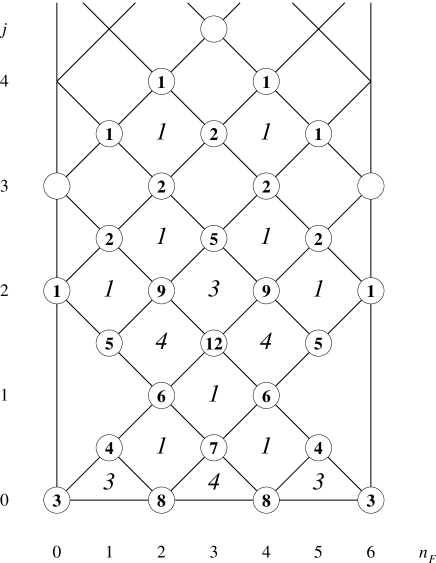
Figure 3: Populations of channels (bold) versus equivalent number of supermultiplets (italics) at $n_{B_{max}}=3$.

Fig. 3 shows such a map together with the number SO(3) multiplets in each channel (for a particular value of a cutoff $n_{B\max}\$). The distribution of states among channels is such that each SO(3) multiplet belongs to one and only one diamond adjacent to the vertex. This ”population” of all vertices determines the multiplicities of individual diamonds, i.e., the number of supermultiplets reproduced at given $n_{B\max}\$. The latter are given in italic in the figure. More precisely, if $R_{I}$ denotes the multiplicity of a diamond I, and $d_{i}$ is a number of SO(3) multiplets in a channel $i=(n_{F},j)$ then

$$d_{i}=\Sigma_{I|i}R_{I},$$ (46)

where $\Sigma_{I|i}$ means summation over I’s adjacent to $i$. These diamonds are nothing but supersymmetric multiplets which will be discussed below in detail. At present stage they play only a kinematical role — they provide an alternative way of classifying all basis states. Our cutoff $n_{B\max}\$ violates supersymmetry, however it violates it rather gently. Namely, for every odd $n_{B\max}\$ the total number of states is such that they fill the integer number of supermultiplets. Taking into account the SO(3) degeneracy, we see immediately that the numbers of fermionic and bosonic states in a diamond match. These last two properties account for the exact balance between fermionic and bosonic states found earlier, cf. the last column of Table 1. For even $n_{B\max}\$, Eq. (46) also holds, but exactly two diamonds at highest $j$ have $d=-1$. However, this does not spoil the exact balance, and it is irrelevant in our perspective of increasing $n_{B\max}\$ at fixed $j$.

We shall discuss now some detailed features of the model which follow from supersymmetry and rotational symmetry.

4.2 The algebra of SUSY generators: supermultiplets

It is convenient to work with the Weyl generators defined in Eq. (30), which carry definite fermionic number $n_{F}$ and angular momentum ($m=\pm{\textstyle{1\over 2}}$), and satisfy the standard anticommutation relations

$$\{Q_{m},Q^{\dagger}_{n}\}=4H\delta_{mn},\quad\{Q^{\dagger}_{m},Q^{\dagger}_{n}\}=\{Q_{m},Q_{n}\}=0$$ (47)

in the gauge-invariant sector.

A supermultiplet can be constructed by considering $Q^{\dagger}_{m}$ as creation operators and $Q_{m}$ as annihilation operators acting on the “vacuum” – the lowest-$n_{F}$ state of the supermultiplet. Starting from a single eigenstate of $H$ with nonzero energy and definite $n_{F}\leq 3$, $j$, and $m$, Eq. (47) implies that exactly three more states are produced: two by acting with $Q^{\dagger}_{{\textstyle{1\over 2}}}$ and $Q^{\dagger}_{-{\textstyle{1\over 2}}}$, with quantum numbers $n_{F}+1$ and $m\pm{\textstyle{1\over 2}}$, and one by acting with $Q^{\dagger}_{{\textstyle{1\over 2}}}Q^{\dagger}_{-{\textstyle{1\over 2}}}-Q^{\dagger}_{-{\textstyle{1\over 2}}}Q^{\dagger}_{{\textstyle{1\over 2}}}$, with quantum numbers $n_{F}+1$, $j$, and and $m$ (since $Q^{\dagger}_{{\textstyle{1\over 2}}}Q^{\dagger}_{-{\textstyle{1\over 2}}}+Q^{\dagger}_{-{\textstyle{1\over 2}}}Q^{\dagger}_{{\textstyle{1\over 2}}}$ vanishes). It is easy to show that applying $Q_{m}$ or $Q^{\dagger}_{m}$ to any of these states either gives zero or another of these states. Starting now from a full rotational multiplet, $Q^{\dagger}_{m^{\prime}}|n_{f},j,m\rangle$ is decomposed into two multiplets with $n_{F}+1$ and $j\pm{\textstyle{1\over 2}}$, ($j-{\textstyle{1\over 2}}$ is absent if $j=0$); additionally, we have one $n_{F},j$ and one $n_{F}+2,j$ multiplet. This structure, which is nothing but a diamond of Sect. 4.1, is shown in Fig. 4.

Figure 4: The diamond structure of a supermultiplet, with supersymmetry fractions $q$.

4.3 Supersymmetry fractions

Applying Eqs. (85) and (88) to Eq. (47), we obtain

$${\langle j;i^{\prime\prime}\|H\|j;i\rangle}=$$

$$\quad{1\over 4\sqrt{2j+1}}\sum_{j^{\prime},i^{\prime}}\left[{\langle j;i^{\prime\prime}\|Q^{\dagger}\|j^{\prime};i^{\prime}\rangle}\,{\langle j;i\|Q^{\dagger}\|j^{\prime};i^{\prime}\rangle}+{\langle j^{\prime};i^{\prime}\|Q^{\dagger}\|j;i^{\prime\prime}\rangle}\,{\langle j^{\prime};i^{\prime}\|Q^{\dagger}\|j;i\rangle}\right].$$ (48)

When $|j;i\rangle$ is an eigenstate of $H$ with eigenvalue $E_{j,i}$ and $i^{\prime\prime}=i$, Eq. (48) reduces to

$$\sum_{j^{\prime},i^{\prime}}\left[\left|{\langle j;i\|Q^{\dagger}\|j^{\prime};i^{\prime}\rangle}\right|^{2}+\left|{\langle j^{\prime};i^{\prime}\|Q^{\dagger}\|j;i\rangle}\right|^{2}\right]=4(2j+1)E_{j,i}.$$ (49)

It is therefore natural to define the “supersymmetry fractions”

$$q(j^{\prime},i^{\prime}|j,i)\equiv{1\over 4E_{j,i}}\left|{\langle j^{\prime};i^{\prime}\|Q^{\dagger}\|j;i\rangle}\right|^{2},$$

which, in the limit of exact supersymmetry, satisfy the sum rule

$$\sum_{j^{\prime},i^{\prime}}[q(j^{\prime},i^{\prime}|j,i)+q(j,i|j^{\prime},i^{\prime})]=2j+1.$$ (50)

Supersymmetry fractions allow an easy classification of states into supermultiplets: $q$ is nonzero only between states belonging to the same supermultiplet. For discrete states, the fractions can be computed explicitly, using Eq. (49) and remembering that $\langle j^{\prime};i^{\prime}\|({\tilde{Q}},Q^{\dagger})_{1}\|j;i\rangle$ vanishes on gauge-invariant states. When no mixing occurs, the resulting fractions are

$$q(n_{F}{+}1,j{+}{\textstyle{1\over 2}}|n_{F},j) = q(n_{F}{+}2,j|n_{F}{+}1,j{+}{\textstyle{1\over 2}})=j+1,$$

$$q(n_{F}{+}1,j{-}{\textstyle{1\over 2}}|n_{F},j) = q(n_{F}{+}2,j|n_{F}{+}1,j{-}{\textstyle{1\over 2}})=j,$$ (51)

(they are also shown in Fig. 4); they saturate Eq. (50).

4.4 The spectrum - cutoff dependence and general properties

Monitoring the cutoff dependence is crucial for at least two reasons. First, it provides a model-independent information about the errors induced by limiting the Hilbert space. Second, it allows to distinguish between localized and non-localized states. The latter feature is particularly useful in studying supersymmetric gauge systems where continuous and discrete spectra are known to coexist. It was shown in Ref. [37] that eigenenergies of non-localized states drop slowly to zero with the cutoff, while the discrete spectrum is characterized by rapid convergence to the finite, “infinite volume” eigenvalues.

In the $(0,0)$ and $(2,0)$ channels our results are identical with those of van Baal, Fig. 2, hence we concentrate on other channels, plotted in Fig. 5. For $n_{F}=1,j={\textstyle{1\over 2}}$ the spectrum is similar to that in the $(0,0)$ channel. The levels are quickly converging and the available cutoff is sufficient to guarantee small errors. Similar situation occurs for higher angular momenta with $n_{F}=1$, e.g., for $j={\textstyle{5\over 2}}$. Some degeneracies are observed, e.g., second and third level of the channel $(n_{F}=1,j={\textstyle{1\over 2}})$. They are not caused by supersymmetry, which connects states from different channels, as was discussed in Sect. 4.2.

Figure 5: Cutoff dependence of the spectrum in a sample of channels.

On the other hand in the $n_{F}=3$ sector we clearly observe both convergent, localized states and slowly falling ones from the continuum. The $j={\textstyle{1\over 2}}$ channel plotted in Fig. 5c is very similar in this respect to the $n_{F}=2,j=0$ channel shown earlier (cf. Fig. 2). Similar behavior is seen for other angular momenta. Again, cutoffs reached with present method allow for quantitative studies of many features of the localized states. Scattering states show much more complexity, nevertheless some of their properties can be also inferred, see below.

We therefore seem to confirm the general pattern suggested already by the low $n_{B\max}\$ calculations: in zero- and one-fermion sectors (and their particle-hole images) the spectrum is discrete, while in the “fermion rich” sectors with $n_{F}=2,3,4$, both localized and non-localized states coexist. There is however additional refinement of this rule.

Contrary to earlier expectations the spectrum is entirely discrete also in the $n_{F}=2,j=1$ channel, Fig. 5d. In fact we observe that this happens in all $n_{F}=2$ channels with odd angular momentum $j$. Therefore previous rule is modified to the following: scattering states exist in the $n_{F}=3$ sector for all angular momenta, while non-localized states with $n_{F}=2$ occur only for even angular momentum. This will find yet simpler interpretation when we discuss in detail the supermultiplet structure of the spectrum.

4.5 Discrete spectrum - identifying supermultiplets

To begin with, let us collect the “spectroscopy” graph of the energy levels with lowest angular momentum in all fermionic sectors, Fig. 6.

Figure 6: Spectrum of the $j=0,{\textstyle{1\over 2}}$ states obtained with highest cutoff available in each fermionic sector, cf. Table 2.

Clearly a number of states in adjacent channels have identical energies (within our cutoff errors) and are therefore good candidates for SUSY partners. Confronting this with the cutoff dependence, Figs. 2, 5, we see that identification of SUSY multiplets is simpler in the discrete part of the spectrum. Restoration of supersymmetry among the non-localized states is more complex and will be discussed later. Still, in order to achieve a complete classification (even of localized states), it is important to analyze together the highest cutoff results, the cutoff dependence, and supersymmetry fractions. This is done below.

Recall from Sect. 4.2 that a supermultiplet of SYMQM is composed by the diamond of O(3) multiplets shown in Fig. 4: $(n_{F},j)$, the multiplet with the lowest $n_{F}$, $(n_{F}{+}1,j{+}{\textstyle{1\over 2}})$, $(n_{F}{+}1,j{-}{\textstyle{1\over 2}})$ (only if $j>0$), and $(n_{F}{+}2,j)$. We will denote the full supermultiplet by the spectroscopic labels $n_{F}(j)$ for the ground state in the channel, $n_{F}(j)^{\prime}$ for the first excited state etc.; when many excited states are considered, we label them by their energies multiplied by $10^{3}$. In the case $n_{F}=0$, when $(-1)^{n_{B}}$ is conserved for the $(0,j)$ multiplet, we add an $n_{B}$-parity label, i.e., we write $0(j^{\pm})$.

We begin the detailed presentation of our data by plotting the energy levels vs. $n_{B\max}$ for several channels in Figs. 7–11. The channels with higher $j$ follow a pattern quite similar to these, and therefore we will not present here the corresponding plots; for the remaining channels with $j\leq 4$, they can be found on the authors’ web site [38]. For the lower levels of each channel, we quote the spectroscopic labels $n_{F}(j)$ identifying the supermultiplet to which the level belongs, anticipating results from the following of the present Section.

Figure 7: Energy levels vs. $n_{B\max}$ for the channel $(0,0)$; solid lines indicate even $n_{B}$-parity, dashed lines odd $n_{B}$-parity.

Figure 8: Energy levels vs. $n_{B\max}$ for the channel $(1,{\textstyle{1\over 2}})$.

Figure 9: Energy levels vs. $n_{B\max}$ for the channel $(2,0)$.

Figure 10: Energy levels vs. $n_{B\max}$ for the channel $(2,1)$.

Figure 11: Energy levels vs. $n_{B\max}$ for the channel $(3,{1\over 2})$.

The most effective tool to classify states into supermultiplets is based on the analysis of supersymmetry fractions; the spectroscopic labels reported in the above-mentioned plots are obtained by the following method.

Let us select two sectors with fixed $(n_{F}^{\prime}=n_{F}{+}1,j^{\prime}=j\pm{\textstyle{1\over 2}})$ and $(n_{F},j)$, and construct the matrix $q(n_{F}^{\prime},j^{\prime},i^{\prime}|n_{F},j,i)$, where $i^{\prime}$ and $i$ run over the energy eigenvalues of the two sectors; the cutoff $n_{B\max}$ is often the same in the two sector, but it may be different, in which case we will write the two cutoffs as $n_{B\max}^{\prime}|n_{B\max}$. Take one $(n_{F}^{\prime},j^{\prime},i^{\prime})$ state and look at the corresponding row of the matrix as $n_{B\max}$ grows: if all elements go to zero, the state belongs to a $(n_{F}^{\prime},j^{\prime})$ supermultiplet. In the same way, take one $(n_{F},j,i)$ state and look at the corresponding column of the matrix: if all elements go to zero, the state belongs to a $(n_{F}{-}2,j)$ supermultiplet. If one element remains nonzero, the two corresponding states belong to the same supermultiplet: we look for the remaining superpartners coupling to these two states in the appropriate channels, forming the diamond of Fig. 4, with the given values of $q$. If two elements remain nonzero, we have a case of “accidental” degeneracy of two supermultiplets: the $q$’s are the superposition of two patterns of Fig. 4, with coefficients $\cos^{2}\theta$ and $\sin^{2}\theta$, where $\theta$ is the mixing angle between the energy eigenstates (which are not exactly degenerate at finite $n_{B\max}$) and the states belonging to a definite supermultiplet. If a number of elements remain nonzero (typically 5 to 10 for our values of $n_{B\max}$), the state belongs to the continuum.

Let us look in details, e.g., at the transition $q(1,{\textstyle{1\over 2}}|0,0^{+})$. The $q$ matrix for our highest value of $n_{B\max}$ is shown in Table 3 for $n_{B\max}=18$; selected coefficients are plotted vs. $n_{B\max}$ in Fig. 12. We identify the states in each channels by their energies at $n_{B\max}=18$ ($n_{B\max}=19$ for $(0,j^{-})$), multiplied by $10^{3}$: we use the notation $(n_{F},j,E)$, or just $E$ when $n_{F}$ and $j$ are obvious.

	$(0,0^{+})$
$(1,1/2)$	4117	6388	7997	9290	10230	11383	12943	13572	14109	14955
4117	1000	0	0	0	0	0	0	0	0	0
6388	0	114	0	0	0	0	0	0	0	0
6401	0	885	0	0	0	0	0	0	0	0
8063	0	0	963	4	1	0	0	0	0	0
8216	0	0	26	2	1	0	0	0	0	0
8789	0	0	0	0	0	0	0	0	0	0
9334	0	0	0	84	0	0	0	0	0	0
9438	0	0	3	877	24	5	0	0	0	0
10273	0	0	0	1	124	0	0	0	0	0
10402	0	0	1	16	817	35	2	0	0	0
11637	0	0	0	0	0	12	0	0	0	0
11726	0	0	0	5	15	662	22	4	0	0
11827	0	0	0	1	4	221	30	9	0	1
12097	0	0	0	0	0	1	0	0	0	0
12344	0	0	0	0	0	0	1	0	0	0
13000	0	0	0	0	1	4	54	1	0	1
13350	0	0	0	0	1	10	611	289	3	18
14037	0	0	0	1	2	15	132	351	19	72
14140	0	0	0	0	0	2	18	44	777	16
14190	0	0	0	0	0	1	8	49	5	5

Table 3: Matrix of supersymmetry fractions $q(1,{\textstyle{1\over 2}}|0,0^{+})$ at $n_{B\max}=18$. States are identified by their energies. All numbers are multipled by $10^{3}$.

Figure 12: Selected supersymmetry fractions $q(1,{\textstyle{1\over 2}},i^{\prime}|0,0^{+},i)$ vs. $n_{B\max}$.

Proceeding by increasing energies, first we see a perfect match for the two ground states, i.e., $q(4117|4117)=1$, and they therefore belong to the $0(0^{+})$ supermultiplet. Next we have a case of mixing: since $q(6388|6388)=0.114$ and $q(6401|6388)=0.885$, $(0,0^{+},6388)$ belongs to $0(0^{+})^{\prime}$, while $(1,{\textstyle{1\over 2}},6388)$ and $(1,{\textstyle{1\over 2}},6401)$ are linear combination of states belonging to the “accidentally” degenerate $0(0^{+})^{\prime}$ and $(1,{\textstyle{1\over 2}})$ supermultiplets, with a mixing angle $\theta$ with $\cos^{2}\theta=0.114$. For higher levels, $q$’s are not completely stable in $n_{B\max}$, and we need to extrapolate them to $n_{B\max}\to\infty$. We clearly see that $(0,0^{+},7997)$ and $(1,{\textstyle{1\over 2}},8063)$ belong to $0(0^{+})^{\prime\prime}$. For higher states, the analysis requires more care.

The remaining members of the $0(0^{+})$ supermultiplets can be identified by looking at $q(2,0,i^{\prime}|1,{\textstyle{1\over 2}},i)$ , which is shown in Table 4 for $n_{B\max}=17|18$: $(2,0,4121)$ belongs to $0(0^{+})$; since $q(6397|6404)\to 0$ and $q(6484|6388)\to 0$, $(2,0,6397)$ and $(2,0,6404)$ are linear combination of states belonging $0(0^{+})^{\prime}$ and $(1,{\textstyle{1\over 2}})$, with the same mixing angle $\theta$ as above. $(2,0,8806)$, despite the high energy, is very easily attributed to $0(0^{-})$, with the help of Table 5. The levels $(2,0,i^{\prime})$ related to the continuum spectrum have zero $q(2,0,i^{\prime}|1,{\textstyle{1\over 2}},i)$.

	$(1,1/2)$
$(2,0)$	4117	6388	6401	8063	8216	8789	9334	9438
237	0	0	0	0	0	0	0	0
1004	0	0	0	0	0	0	0	0
2216	0	0	0	0	0	0	0	0
3777	0	0	0	0	0	0	0	0
4119	1000	0	0	0	0	0	0	0
5188	0	0	0	0	0	0	0	0
5345	0	0	0	0	0	0	0	0
6024	0	0	0	0	0	0	0	0
6394	0	556	34	0	0	0	0	0
6459	0	1	903	3	0	0	0	0
7372	0	0	0	0	0	0	0	0
7468	0	0	0	2	1	0	0	0
8177	0	0	1	667	82	0	1	3
8317	0	0	1	253	192	0	2	14
8396	0	0	0	29	228	0	1	8
8798	0	0	0	0	0	999	0	0
8817	0	0	0	1	0	0	2	0
9369	0	0	0	0	0	0	165	7
9422	0	0	0	1	1	0	352	18
9693	0	0	0	8	3	0	7	819

Table 4: Matrix of supersymmetry fractions $q(2,0|1,{\textstyle{1\over 2}})$ at $n_{B\max}=18$.

	$(0,0^{-})$
$(1,1/2)$	8787	12063	14064
4117	0	0	0
6388	0	0	0
6401	0	0	0
8063	0	0	0
8216	0	0	0
8789	1000	0	0
9334	0	0	0
9438	0	0	0
10273	0	0	0
10402	0	0	0
11637	0	0	0
11726	0	1	0
11827	0	0	0
12097	0	990	1
12344	0	5	0

Table 5: Matrix of supersymmetry fractions $q(1,{1\over 2}|0,0^{-})$ at $n_{B\max}=18|19$.

We then look at $q(2,1,i^{\prime}|1,{\textstyle{1\over 2}},i)$ and $q(3,{\textstyle{1\over 2}},i^{\prime}|2,0,i)$ to identify the remaining members of the $1({\textstyle{1\over 2}})$ supermultiplets. $q(2,1,i^{\prime}|1,{\textstyle{1\over 2}},i)$, presented in Table 6, presents the same pattern as $q(2,0,i^{\prime}|1,{\textstyle{1\over 2}},i)$, except for the absence of continuum states, and we will not delve into the classification of states.

	$(1,1/2)$
$(2,1)$	4117	6388	6401	8063	8216	8789	9334	9438	10273	10402	11637
4692	0	0	0	0	0	0	0	0	0	0	0
5783	0	0	0	0	0	0	0	0	0	0	0
6019	0	0	0	0	0	0	0	0	0	0	0
6395	0	1328	171	0	0	0	0	0	0	0	0
6971	0	0	0	0	0	0	0	0	0	0	0
7744	0	0	0	0	0	0	0	0	0	0	0
7899	0	0	0	0	0	0	0	0	0	0	0
8275	0	0	0	42	1440	0	6	0	4	0	0
8700	0	0	0	0	0	0	0	0	0	0	0
9027	0	0	0	0	0	0	0	0	0	0	0
9400	0	0	0	0	3	0	1341	124	22	0	0
9583	0	0	0	0	0	0	0	0	0	0	0
9710	0	0	0	0	0	0	0	0	0	0	0
9817	0	0	0	0	0	0	0	0	0	0	0
10042	0	0	0	0	0	0	0	0	0	0	0
10129	0	0	0	0	0	0	0	0	0	0	0
10526	0	0	0	0	2	0	16	0	1231	167	3
10817	0	0	0	0	0	0	0	0	0	0	0
11183	0	0	0	0	0	0	0	0	0	0	0
11352	0	0	0	0	0	0	0	0	0	0	0
11475	0	0	0	0	0	0	0	0	0	0	0
11652	0	0	0	0	0	0	0	0	0	0	1446
11696	0	0	0	0	0	0	0	0	0	0	0

Table 6: Matrix of supersymmetry fractions $q(2,1|1,{\textstyle{1\over 2}})$ at $n_{B\max}=18$.

$q(3,{\textstyle{1\over 2}},i^{\prime}|2,0,i)$, shown in Table 7, presents a new, very interesting pattern: we see states with a broad distribution of $q$’s quite different from zero, even with states with very different energies; looking at the $n_{B\max}$ dependence of the levels, cf. Figs. 9 and 11, we conclude that the patterns identifies continuum levels. On the other hand, $q$ is zero between continuum and discrete states, or between discrete states of significantly different energies. We can easily identify members of supermultiplets with quantum numbers $0(0)$, $1({\textstyle{1\over 2}})$, $2(0)$, and $2(1)$, with the remaining states belonging to the continuum. The “doubling” of $(3,{\textstyle{1\over 2}})$ states belonging to $1({\textstyle{1\over 2}})$ supermultiplets is due to the particle-hole symmetry, as will be explained below.

	$(2,0)$
$(3,1/2)$	237	1004	2216	3777	4119	5188	5345	6024	6394	6459	7372	7468
513	737	220	11	1	0	0	0	0	0	0	0	0
1526	73	538	280	15	0	0	1	0	0	0	0	0
2924	12	43	476	301	0	0	13	6	0	0	1	0
4592	1	6	34	449	0	0	275	68	0	0	8	2
5187	0	0	0	0	0	999	0	0	0	0	0	0
5669	0	0	3	21	0	0	500	414	0	0	10	2
6015	0	0	0	0	0	0	0	0	0	0	0	0
6419	0	0	0	0	0	0	0	0	204	44	0	0
6434	0	0	0	0	0	0	1	2	203	43	2	1
6721	0	1	4	22	0	0	86	359	2	1	246	84
7425	1	0	0	0	0	0	0	0	0	0	219	750
7800	0	0	0	4	0	0	12	30	0	0	385	71
7839	0	0	0	0	0	0	0	0	0	0	0	0
8422	0	0	0	0	0	0	0	0	0	0	1	3

Table 7: Matrix of supersymmetry fractions $q(3,{\textstyle{1\over 2}}|2,0)$ at $n_{B\max}=18$.

It is also worth presenting $q(3,{\textstyle{1\over 2}},i^{\prime}|2,1,i)$, shown in Table 8; thanks to the absence of continuum states from $(2,1)$, it is very easy to identify states in $(3,{\textstyle{1\over 2}})$ belonging to the supermultiplets $1({\textstyle{1\over 2}})$ and $2(1)$.

	$(2,1)$
$(3,1/2)$	4692	5783	6019	6395	6971	7744	7899	8275	8700	9027	9400	9583
513	0	0	0	0	0	0	0	0	0	0	0	0
1526	0	0	0	0	0	0	0	0	0	0	0	0
2924	0	0	0	0	0	0	0	0	0	0	0	0
4592	0	0	0	0	0	0	0	0	0	0	0	0
5187	0	0	0	0	0	0	0	0	0	0	0	0
5669	0	0	0	0	0	0	0	0	0	0	0	0
6015	0	0	999	0	0	0	0	0	0	0	0	0
6419	0	0	0	748	0	0	0	1	0	0	0	0
6434	0	0	0	744	0	0	0	1	0	0	0	0
6721	0	0	0	3	0	0	0	1	0	0	0	0
7425	0	0	0	0	0	0	0	5	0	0	0	0
7800	0	0	0	0	0	0	0	8	0	0	0	0
7839	0	0	0	0	0	21	964	0	1	0	0	1
8422	0	0	0	0	0	0	0	721	0	0	8	0
8489	0	0	0	1	0	0	0	641	0	0	16	0
8693	0	0	0	0	0	0	0	60	0	0	15	0
9267	0	0	0	0	0	0	0	0	0	0	2	0
9317	0	0	0	0	0	0	0	1	0	0	125	0
9441	0	0	0	0	0	0	4	0	4	3	0	678
9529	0	0	0	0	0	0	0	8	0	0	594	0
9554	0	0	0	0	0	0	0	15	0	0	682	0
9898	0	0	0	0	0	0	0	0	0	0	1	0

Table 8: Matrix of supersymmetry fractions $q(3,{\textstyle{1\over 2}}|2,1)$ at $n_{B\max}=18$.

The analysis of $q$ for higher $j$ is repeated exactly in the same way. We will not present here the corresponding $q$ matrices, which can be found in Ref. [38] for the remaining channels with $j\leq 4$. We only remark that all $q(n_{F}^{\prime},j^{\prime}|n_{F},j)$ for the same values of $n_{F}^{\prime},n_{F}$ and different values of $j^{\prime},j$ are qualitatively very similar (in the case of $n_{F}^{\prime}=2$ ($n_{F}=2$), only for $j^{\prime}$ ($j$) having the same parity).

From all the above data, we can compile the spectroscopy of Tables 9 and 10. The table is limited to $n_{F}\leq 2$, since the other supermultiplets can be obtained by particle-hole reflection, and to $j\leq 4$, since nothing new happens for higher $j$.

One feature should be stressed: for each $1(j)$ supermultiplet, the particle-hole symmetry implies the existence of a conjugate supermultiplet $3(j)$, and therefore of two $(3,j)$ states of degenerate energy (in the $n_{B\max}\to\infty$ limit); we observe mixing of each pair, with a mixing angle $\theta=\pi/4$.

Figure 13 shows a sample of the lowest supermultiplets for the first few angular momenta and all $n_{F}$. Degenerate supermultiplets at $E\sim 6.4$ and $8.1$ were slightly split for the sake of illustration.

$10^{3}{\times}$energies at $n_{B\max}=18$
$n_{F}(j)$	$(n_{F},j)$	$(n_{F}{+}1,j{-}{\textstyle{1\over 2}})$	$(n_{F}{+}1,j{+}{\textstyle{1\over 2}})$	$(n_{F}{+}2,j)$
$0(0^{+})$	04117	—	04117	04119
$0(0^{+})^{\prime}$	06388	—	6388, 6401	6394, 6459
$0(0^{+})^{\prime\prime}$	07997	—	08063	08177
$0(0^{+})_{9290}$	09290	—	9334, 9438
$0(0^{+})_{10230}$	10230	—	10402
$0(0^{+})_{11383}$	11383	—	11726
$0(0^{+})_{12943}$	12943	—
$0(0^{-})$	08787	—	08789	08798
$0(0^{-})^{\prime}$	12063	—	12097
$0(2^{+})$	06015	06019	06020	06041
$0(2^{+})^{\prime}$	07839	07899	07902	08071
$0(2^{+})^{\prime\prime}$	09441		09628
$0(2^{+})_{9961}$	09961
$0(2^{+})_{11183}$	11183
$0(2^{+})_{12096}$	12096
$0(2^{+})_{13005}$	13005
$0(2^{-})$	11334	11352	11355	11407
$0(2^{-})^{\prime}$	14045	14131	14187
$0(3^{+})$	12138	12174	12178	12230
$0(3^{+})^{\prime}$	15068
$0(3^{+})^{\prime\prime}$	17647
$0(3^{+})_{19294}$	19294
$0(3^{-})$	18140	18395	18663
$0(4^{+})$	07739	07768	07772	07863
$0(4^{+})^{\prime}$	09411	09603	09604
$0(4^{+})^{\prime\prime}$	11153
$0(4^{+})_{12603}$	12603
$0(4^{+})_{13152}$	13152
$0(4^{+})_{14364}$	14364
$0(4^{-})$	13747	13824	13841	13948

Table 9: Spectroscopy of SYMQM.

$10^{3}{\times}$energies at $n_{B\max}=18$
$n_{F}(j)$	$(n_{F},j)$	$(n_{F}{+}1,j{-}{\textstyle{1\over 2}})$	$(n_{F}{+}1,j{+}{\textstyle{1\over 2}})$	$(n_{F}{+}2,j)$
$1(1/2)$	6388, 6401	6394, 6459	06395	6419, 6434
$1(1/2)^{\prime}$	08216	08317	08275	8422, 8489
$1(1/2)^{\prime\prime}$	9334, 9438
$1(1/2)_{10273}$	10273
$1(3/2)$	04692	04692	04694	4694, 4696
$1(3/2)^{\prime}$	05783	05783	05791	5790, 5799
$1(3/2)^{\prime\prime}$	06971	06971	07008	7010, 7047
$1(3/2)_{7744}$	07744	07744	07809	7826, 7839
$1(3/2)_{8700}$	08700	08700	08782	8831, 8908
$1(5/2)$	06486	06484	06501	6488, 6508
$1(5/2)^{\prime}$	07733	07751	07763	7808, 7866
$1(5/2)^{\prime\prime}$	08379	08386	8420, 8527∗	8411, 8485
$1(5/2)_{9352}$	09352
$1(7/2)$	06591	06593	06611	6613, 6628
$1(7/2)^{\prime}$	07515	07518	07553	7546, 7578
$1(7/2)^{\prime\prime}$	08428	8420, 8527∗	08548	8579, 8654
$1(7/2)_{9314}$	09314
$2(0)$	05188	—	05187	05188
$2(0)^{\prime}$	07373	—	07444	07425
$2(1)$	06019	06015	06028	06019
$2(1)^{\prime}$	07899	07839	08006	07899
$2(2)$	06734	06722	06736	06734
$2(3)$	06085	06079	06093	06085
$2(3)^{\prime}$	07826	07800	07876	07826
$2(3)^{\prime\prime}$	08208	08168	08304	08208
$2(4)$	08169	08140		08169

Table 10: Spectroscopy of SYMQM (continued).
^∗ The two states $(2,3,8420)$ and $(2,3,8527)$ belong to supermultiplets with different energies, but appear to be mixed at the available values of $n_{B\max}$.

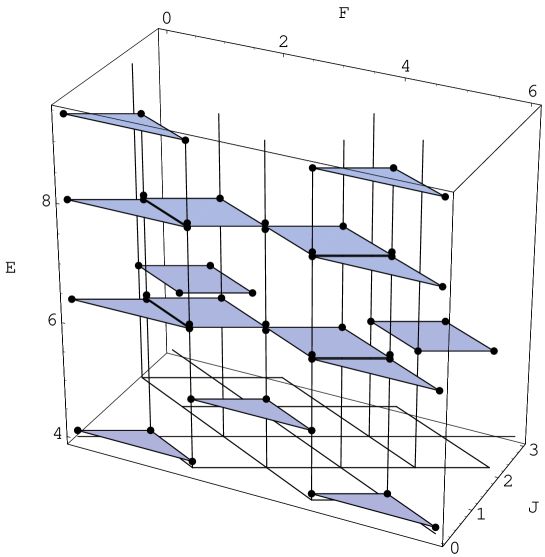
Figure 13: Spectrum of a sample of supermultiplets identified in Tables 9 and 10

4.6 Continuous spectrum

We already mentioned that a continuous spectrum is observed for all $j$’s in the $n_{F}=3$ channels, but only for even angular momenta in the $n_{F}=2,4$ sectors. This pattern is consistent with supersymmetry, and simply means that continuous states exist only in supermultiplets $2(j)$ with even $j$. Note that the “opposite” behaviour (all $n_{F}=2$ channels and every second $n_{F}=3$ channel) cannot be accommodated into a geometric structure of supermultiplets, cf. Fig. 3.

It is also interesting to realize that, even though supersymmetry is broken by the cutoff, the above rule is not, i.e., we don’t see any hint of continuum states in the channels $(n_{f}=2,4,j=odd)$ for any finite cutoff.

4.6.1 Scaling

Non-localized states of the system describe D-particles [13] penetrating the flat directions of the potential, as mentioned in the Introduction. In a cut system all energy levels of the continuum states fall to zero with increasing $n_{B\max}\$. If we label them by a “principal quantum number” $m$, the large-cutoff limit at fixed $m$ is trivial. Such a phenomenon was also found in the free case when one regularizes the system by limiting the number of quanta [37]. In that case, it was also shown that the nontrivial and correct continuum limit is the scaling limit

$$E(p)=\lim_{N\rightarrow\infty}E^{m(N,p)}_{N},\;\;m=\frac{p}{\pi}\sqrt{2N}.$$ (52)

where $p$ is the continuum momentum and $N$ the cutoff. These results were obtained analytically for a free particle in one dimension. They also apply to the $D=2$ SU(2) SYMQM, since this is effectively a quantum mechanics of a free particle in three (color) dimensions, projected on the singlet and triplet channels of angular momentum [39]. The present, $D=4$, case is more complicated. However, we expect that, whenever it is possible to define asymptotic states with given momentum, as is the case for the scattering process considered here, some version of Eq. (45) should hold. Scattering states in the present model correspond to particles propagating freely in the three dimensional (color) flat valleys of the potential $V$, cf. Eq. (6). Gauge invariance restricts color orbital angular momentum to few channels, so we are not that far from the $D=2$ example. We have therefore taken Eq. (52) as a phenomenological rule and tested it with our data.

Figure 14: Eigenenergies of the first three levels from the continuum, in the $(n_{F}=3,j=1/2)$ channel, multiplied by $n_{B\max}\$, as the function of the cutoff.

The scaling limit (52) implies that at fixed $m$ all energies of non-localized states behave as ${\rm O}(1/N)$. Figure 14 tests this prediction assuming that we identify the one dimensional cutoff $N$ with $n_{B\max}\$. Indeed the energies of the first four levels seem to follow $1/n_{B_{max}}$ behavior both in $n_{F}=2$ and $n_{F}=3$ sectors. We did not use higher levels since they are probably influenced by the the discrete spectrum.

One can also contrast the $m$ dependence with the one dimensional formula

$$E^{(m)}_{N}=\frac{\pi m^{2}}{4N},$$ (53)

and with the $D=2$ case. Table 11 compares ratios of our first four energy levels, for the largest value of the cutoff, with analogous ratios of the $D=2$ system at the same value of $N$, and with Eq. (53).

$E^{(k)}/E^{(m)}$	$D=4$	$D=2$	exact
	$n_{F}=2,\ j=0$	$n_{F}=0$	$\frac{k^{2}}{m^{2}}$
$E^{(2)}/E^{(1)}$	4.24	4.02	4.00
$E^{(3)}/E^{(1)}$	9.32	9.13	9.00
$E^{(3)}/E^{(2)}$	2.20	2.27	2.25
$E^{(4)}/E^{(1)}$	15.97	16.46	16.00
$E^{(4)}/E^{(2)}$	3.76	4.09	4.00
$E^{(4)}/E^{(3)}$	1.70	1.80	1.78
	$D=4$	$D=2$
	$n_{F}=3,\ j=1/2$	$n_{F}=1$	$N=150$
$E^{(2)}/E^{(1)}$	2.97	2.98	2.96
$E^{(3)}/E^{(1)}$	5.67	6.11	5.89
$E^{(3)}/E^{(2)}$	1.90	2.01	1.99
$E^{(4)}/E^{(1)}$	8.77	10.18	9.81
$E^{(4)}/E^{(2)}$	2.94	3.42	3.32
$E^{(4)}/E^{(3)}$	1.54	1.69	1.66

Table 11: Ratios of the energies from the continuum. Comparisons between the $D=2$ and $D=4$ systems.

The comparison is done in two channels: the $(2,0)$ channel, corresponding to the bosonic $n_{F}=0$ sector of the $D=2$ model, and the $(3,1/2)$ channel, which is the counterpart of the fermionic $n_{F}=1$ sector. To give an idea of the cutoff effects, we quote the $D=2$ energies for $N=18=n_{B\max}$ (third column) and for $N=150$, which is easily available in this case and coincides with $N=\infty$ within the two digits accuracy reported (fourth column, lower half).

In the scalar case, high-cutoff results for $D=2$ are identical with the exact ratios $k^{2}/m^{2}$. The one-dimensional formula (53) does not apply to the fermionic sector. It is not surprising since this case corresponds to color angular momentum $j=1$ and the three dimensional Schrödinger equation coincides with the one dimensional one only for $j=0$.

Finally, the comparison of the ratios for $D=4$ with $D=2$ is rather satisfactory. Numerical values of the energy ratios for the two systems are quite similar, over a range of an order of magnitude. All discrepancies are consistent with the cutoff effects. However one cannot exclude differences $\sim 10\%$ and consequently higher $n_{B\max}\$ are required for more quantitative conclusions.

4.6.2 Dispersion relation

An interesting question appears whether the dispersion relation for the scattering states has the standard parabolic form, or whether it is modified by rather unusual behaviour of the potential. With the help of the scaling relation (52) we can now address this issue in both bosonic and fermionic sectors. For $n_{F}=2,j=0$ the dispersion relation was first obtained by van Baal [35].

Figure 15: Dispersion relation for the lowest three scattering states in the $(2,0)$ and $(3,1/2)$ channels.

In Fig. 15 we have plotted the first three energy levels, as a function of $m/\sqrt{n_{B_{max}}}$, for both bosonic ($n_{F}=2,j=0$) and fermionic $(n_{F}=3,j=1/2)$ channels. Points from different $m$ and $n_{B\max}\$ follow roughly a common curve which again confirms approximately the scaling relation (52). Moreover, when the proper normalization of the momentum, required in (52), is taken into account, one obtains a reasonable agreement with the standard $p^{2}/2$ kinetic energy of one degree of freedom (solid lines).

Many effects prevent us from reaching better agreement at the moment. For example, the repulsion of the lowest discrete state at $E=4.12$ is clearly seen in the (2,0) channel, while it is not as efficient in (3,1/2), where the lowest state is higher ($E=5.19$). For the present values of $n_{B\max}\$, only the three lowest states can be used, hence one expects non-leading corrections in $m$. The identification of $N$ with $n_{B\max}\$ should be more carefully examined, etc. However, keeping in mind all these limitations, the overall picture seems reasonably satisfactory and we are looking forward for better data to make more extensive study of these points.

4.7 Witten index

With complete diagonalization of the Hamiltonian achieved in all sectors we can now calculate the regularized Witten index directly from the definition

$$I_{W}(T)=\sum_{i}(-1)^{n_{F}(i)}e^{-TE(i)}.$$

The results, shown in Fig. 16, nicely confirm and strengthen early expectations based on much smaller $n_{B\max}\$.

Figure 16: Regularized Witten index $I_{W}(T)$ vs. $T$ for even (left) and odd (right) $n_{B\max}\leq 17$ .

As already mentioned, the number of bosonic and fermionic states is the same for any value of the cutoff, be it even or odd. Therefore the index vanishes at $T=0$ with this regularization. The sharp structure around $T=0$ clearly moves toward the origin with increasing cutoff indicating singularity at infinite $n_{B\max}$. Such a discontinuity is expected on general grounds and finds a reasonable support here.

Of course at high $T$ our “cut” index is bound to vanish exponentially. However there exist a range of intermediate times where definite flattening occurs. This signals effective cancellations among supersymmetric partners hence a gradual, global restoration of SUSY. Moreover the plateau seems to converge to ${\textstyle{1\over 4}}$ — a known result obtained also from the non-abelian integrals for the SU(2) gauge group [9] - [11].

In order to study the large cutoff limit more quantitatively we have performed a number of extrapolations assuming various asymptotic behaviors of the regularized index in $n_{B\max}\$. For example, Fig. 17 shows the asymptotic value extracted with the aid of the diagonal Padè approximant $P_{[4,4]}(n_{B\max}^{2})$ at various $T$. Two lines correspond to even and odd $n_{B\max}\$cases, which were independently analyzed . Both extrapolations are stable and consistent in the range $1<T<5$. This result strongly suggests that the infinite $n_{B\max}\$limit of the regularized index is time independent. Moreover, the limiting value is nicely consistent with the above $1/4$ (also shown in the Figure). Extrapolations with power series in different variables lead to similar conclusions. We expect to accumulate new data with yet higher cutoffs. This would allow to extend stable extrapolations to larger range of $T$ and possibly distinguish between various asymptotic forms tested so far.

Figure 17: Infinite $n_{B\max}\$limit of the index deduced from the Padè approximants.

5 Summary and outlook

The next step in studying a family of supersymmetric Yang-Mills quantum mechanics has been completed. The above models appear in many areas of theoretical physics, beginning with the soluble $D=2$ systems, through the small volume, lattice studies of the $D=4$ QCD, and finally ending on the $D=10$ models of the M-theory. We are now somewhere in the middle of this list.

The new approach presented here leads to the precise study of the rich structure of the $D=4$ system, which already has some features of the $D=10$ model. With rotational invariance taken fully into account, the Hilbert space splits into channels of conserved angular momentum and fermionic number. This eliminates the brute force diagonalization of large matrices. Second improvement is brought by the generalization of the recursive scheme of computing matrix elements while gradually increasing the harmonic oscillator basis [23]. Present results fully confirm and extend findings of the first paper where the whole program was originated [6].

The system has both discrete and continuous spectrum which coexist at the same energies. This rather unusual feature was expected for a long time as a consequence of the supersymmetric interactions with flat directions. Now however, more precise statements can be made. While the discrete, localized states exist in all $(n_{F},j)$ channels, the non-localized ones appear only in the central (with respect to the particle-whole reflection) supermultiplets and only for even angular momenta.

The numerical part of the method requires limiting the Hilbert space. We take as a cutoff the maximal number of quanta of all bosonic harmonic oscillators, $n_{B\max}$. The present approach allows to reach such a large cutoffs that the lower part of the discrete spectrum has practically converged to its continuum (i.e., the infinite cutoff) limit.

On the other hand the eigenenergies from the continuous spectrum literally never converge to their continuum values. Instead, they all fall to zero with increasing cutoff. In fact, this is precisely the property allowing a clear distinction of the two spectra, cf. Figs 2 and 5. The physical energies of the non-localized states are coded in the rate of fall of the above levels with $n_{B\max}$. The particular scaling which governs this behavior was discovered some time ago [37] and is well confirmed with present data. It is an important tool in extracting any observable related to the non-localized states. In particular it allowed us to establish the dispersion relation for the scattering states in the $(n_{F}=2,j=0)$ and $(n_{F}=3,j={\textstyle{1\over 2}})$ channels.

Supersymmetry is broken by the cutoff. Again however, with currently available values of $n_{B\max}$, we observe clear restoration of SUSY which manifests itself in many ways in the discrete spectrum. First, the energy levels from different channels, related by supersymmetry, coincide to high accuracy, cf. Fig. 6 . Second, our approach allows to form and analyze the supersymmetric images of arbitrary eigenstates. This led to the construction of the rotationally invariant supersymmetry fractions which provided a simple identification of SUSY partners. A number of lower supermultiplets was identified for a range of angular momenta, see Tables 9 and 10. Interestingly some of the supermultiplets are degenerate, see Fig. 13. We do not know a symmetry (if any) responsible for this additional degeneracy. The mixing angles are stable with respect to changing the cutoff. Their actual values, however, may be an artefact of our regularization.

A third method to see restoration of supersymmetry is provided by the Witten index. It is clearly flattening as a function of euclidean time when we move towards bigger cutoffs which are now available. This shows that the cancellations between supersymmetric partners becomes more and more efficient, also globally. At infinite cutoff contribution from localized states would be exactly zero. Supersymmetric vacuum and other non-localized states should give the final non-integer value 1/4 for the gauge group considered here. We see now much stronger evidence for this behavior than in the first attempts.

In the continuous sector of the theory the situation is more difficult and challenging. Although the scaling expected from the one dimensional free case has been confirmed, it should be studied now more extensively, also for higher angular momenta. Identification of the supermultiplets is more delicate and remains to be done. Similarly revealing a signature of the SUSY vacuum requires further study and yet higher cutoffs. On the other hand current precision allows to address more advanced problems like the scattering [19, 20]. We are looking forward to work out some of these questions.

Progress towards higher $n_{B\max}$ for the $D=4$ system is limited by computer time. The recursive algorithm is presently implemented in Mathematica. We re-implemented some sections of the algorithm in C++, obtaining a 100-fold increase in speed; we plan to complete the C++ implementation and to improve the present computation.

Altogether the present approach works rather well. As such it provides one route of attacking higher dimensions. The gain from exploiting fully SO($D{-}1$) invariance and restricting ourself to a particular representation of SO($D{-}1$) should overcome the huge sizes of bases in higher dimensions. Generalization to $D=10$ requires in particular construction of the Clebsch-Gordan coefficients for the SO(9) group which is a reasonably tedious but a well defined exercise. Some work in this direction has already begun.

Acknowledgments. We would like to thank P. van Baal for discussions and for providing the data for Fig.2. This work is supported by the Polish Committee for Scientific Research under the grants no. 2 P03B 096 22 (2002-2004) and 1  P03B 024 27 (2004-2007), and by INFN under IS PI12.

Appendix A Useful identities involving Clebsch-Gordan coefficients, $\bm{3j}$ symbols, and $\bm{6j}$ symbols

With the usual phase conventions, the Clebsch-Gordan coefficients $C^{j_{1}\,j_{2}\,j}_{m_{1}m_{2}m}$ are real and

$$C^{j\,j\,0}_{m_{1}m_{2}0}={(-1)^{j-m_{1}}\over\sqrt{2j+1}}\,\delta_{m_{1}+m_{2},0};$$ (54)

the completeness formulae read

$$\sum_{j,m}C^{j_{1}\,j_{2}\,j}_{m^{\prime}_{1}m^{\prime}_{2}m}C^{j_{1}\,j_{2}\,j}_{m_{1}m_{2}m}=\delta_{m^{\prime}_{1}m_{1}}\delta_{m^{\prime}_{2}m_{2}},\qquad\sum_{m_{1},m_{2}}C^{j_{1}\,j_{2}\,j^{\prime}}_{m_{1}m_{2}m^{\prime}}C^{j_{1}\,j_{2}\,j}_{m_{1}m_{2}m}=\delta_{m^{\prime}m}\delta_{j^{\prime}j}.$$ (55)

The Clebsch-Gordan coefficients can be written in terms of the Wigner $3j$ symbols as

$$C^{j_{1}\,j_{2}\,j}_{m_{1}m_{2}m}=(-1)^{j_{1}-j_{2}+m}\,\sqrt{2j+1}\left(\begin{array}[]{ccc}j_{1}&j_{2}&j\\ m_{1}&m_{2}&-m\end{array}\right);$$ (56)

the $3j$ symbols enjoy the symmetry properties

$$\left(\begin{array}[]{ccc}j_{2}&j_{1}&j_{3}\\ m_{2}&m_{1}&m_{3}\end{array}\right) = (-1)^{j_{1}+j_{2}+j_{3}}\left(\begin{array}[]{ccc}j_{1}&j_{2}&j_{3}\\ m_{1}&m_{2}&m_{3}\end{array}\right),$$ (61)

$$\left(\begin{array}[]{ccc}j_{2}&j_{1}&j_{3}\\ -m_{1}&-m_{2}&-m_{3}\end{array}\right) = (-1)^{j_{1}+j_{2}+j_{3}}\left(\begin{array}[]{ccc}j_{1}&j_{2}&j_{3}\\ m_{1}&m_{2}&m_{3}\end{array}\right);$$ (66)

we also need the formula [40]

$$\sum_{m_{4},m_{5},m_{6}}(-1)^{j_{4}+j_{5}+j_{6}-m_{4}-m_{5}-m_{6}}\left(\begin{array}[]{ccc}j_{1}&j_{5}&j_{6}\\ m_{1}&-m_{5}&m_{6}\end{array}\right)\left(\begin{array}[]{ccc}j_{4}&j_{2}&j_{6}\\ m_{4}&m_{2}&-m_{6}\end{array}\right)\left(\begin{array}[]{ccc}j_{4}&j_{5}&j_{3}\\ -m_{4}&m_{5}&m_{3}\end{array}\right)$$ (73)

$$\qquad=\left(\begin{array}[]{ccc}j_{1}&j_{2}&j_{3}\\ m_{1}&m_{2}&m_{3}\end{array}\right)\left\{\begin{array}[]{ccc}j_{1}&j_{2}&j_{3}\\ j_{4}&j_{5}&j_{6}\end{array}\right\},$$ (78)

where the term in braces is the Racah $6j$ symbol. Eqs. (56), (61), and (66) imply the “exchange” formulae

$$C^{j_{2}\,j_{1}\,j}_{m_{2}m_{1}m}=(-1)^{j_{1}+j_{2}-j}\,C^{j_{1}\,j_{2}\,j}_{m_{1}m_{2}m},\qquad C^{j_{1}\,j\,j_{2}}_{m_{1}mm_{2}}=(-1)^{j-j_{2}-m_{1}}\,\sqrt{2j_{2}+1\over 2j+1}\,C^{\;j_{1}\,j_{2}\,j}_{-m_{1}m_{2}m},$$ (79)

and the “inversion” formula

$$C^{j_{2}\ j_{1}\ j}_{-m_{2}\,{-}m_{1}\,{-}m}=(-1)^{j_{1}+j_{2}-j}\,C^{j_{1}\,j_{2}\,j}_{m_{1}m_{2}m};$$ (80)

Eq. (78) implies

$$\sum_{m_{4},m_{5},m_{6}}C^{j_{4}\,j_{5}\,j_{1}}_{m_{4}m_{5}m_{1}}\,C^{j_{4}\,j_{6}\,j_{3}}_{m_{4}m_{6}m_{3}}\,C^{j_{5}\,j_{2}\,j_{6}}_{m_{5}m_{2}m_{6}}$$

$$\qquad=(-1)^{j_{2}+j_{3}+j_{4}+j_{5}}\,\sqrt{(2j_{1}+1)(2j_{6}+1)}\left\{\begin{array}[]{ccc}j_{1}&j_{2}&j_{3}\\ j_{6}&j_{4}&j_{5}\end{array}\right\}C^{j_{1}\,j_{2}\,j_{3}}_{m_{1}m_{2}m_{3}}.$$ (83)

Appendix B Computation of matrix elements of products of operators

We wish to exploit rotation invariance to reduce the number of matrix elements which must be computed and stored; our main tool is the Wigner-Eckhart theorem:

$$\langle j^{\prime},m^{\prime};i^{\prime}|{\cal O}^{(1)}_{j_{1},m_{1}}|j,m;i\rangle={1\over\sqrt{2j^{\prime}+1}}\,C^{j_{1}\,j\,j^{\prime}}_{m_{1}mm^{\prime}}{\langle j^{\prime};i^{\prime}\|{\cal O}^{(1)}_{j_{1}}\|j;i\rangle},$$ (84)

where $\langle j^{\prime};i^{\prime}\|{\cal O}^{(1)}_{j_{1}}\|j;i\rangle$ denotes a reduced matrix element, independent on $m^{\prime}$, $m_{1}$, and $m$.

A first formula regarding reduced matrix element can be easily obtained applying Eqs. (79) and (80):

$${\langle j^{\prime};i^{\prime}\|{\tilde{\cal O}}_{j_{1}}\|j;i\rangle}=(-1)^{j_{1}+j-j^{\prime}}\,{\langle j;i\|{\cal O}^{\dagger}_{j_{1}}\|j^{\prime};i^{\prime}\rangle},\qquad{\tilde{\cal O}}_{j,m}=(-1)^{j+m}\,{\cal O}_{j,-m}.$$ (85)

A second formula deals with the product of two operators ${\cal O}^{(1)}_{j_{1},m_{1}}$ and ${\cal O}^{(2)}_{j_{2},m_{2}}$ with given bosonic and fermionic number: by decomposing the of the product in components with definite $\bm{J}^{2}$ and then applying Eq. (83), we obtain

$${\langle j^{\prime};i^{\prime}\|\bigl{(}{\cal O}^{(1)}_{j_{1}},{\cal O}^{(2)}_{j_{2}}\bigr{)}_{j_{3}}\|j;i\rangle}$$

$$\quad=\sum_{j^{\prime\prime},i^{\prime\prime}}(-1)^{j+j^{\prime}+j_{1}+j_{2}}\,\sqrt{2j_{3}+1}\left\{\begin{array}[]{ccc}j_{3}&j&j^{\prime}\\ j^{\prime\prime}&j_{1}&j_{2}\end{array}\right\}{\langle j^{\prime};i^{\prime}\|{\cal O}^{(1)}_{j_{1}}\|j^{\prime\prime};i^{\prime\prime}\rangle}\;{\langle j^{\prime\prime};i^{\prime\prime}\|{\cal O}^{(2)}_{j_{2}}\|j;i\rangle}.$$ (88)

Applying Eqs. (85) and (88), we never need to deal explicitly with $m$’s and Clebsch-Gordan coefficients, and the computations are much more efficient.

(Anti)commutators of operators are dealt with in a very similar way.

Appendix C Implementation of the algorithm

We implemented our algorithms in the symbolic manipulation program Mathematica.

We first compute tables of all needed (anti)commutators and decompositions of products of two trilinear operators into products of three bilinear operators: we define an explicit and univocal representation of a generic operator in terms of $a$, $a^{\dagger}$, $f$, $f^{\dagger}$, in a “canonical” order; using this representation, we compute explicitly the desired operators and decompose them in the appropriate basis of gauge-invariant operators. The computation so far is exact, and the coefficients are square roots of rational numbers. Many checks are performed: besides verifying the rotational properties, we check explicitly Eqs. (26), (27), (29), (31), and (32). This step requires moderate computer resources. Once the tables are computed, the explicit representation of the gauge-invariant operators is no longer needed.

A separate program reads in the tables and implements the orthonormalization and recursive computation of scalar products and matrix elements described in Sects. 3.4 and 3.5. The formulae given in the two sections, together with Hermiticity and decompositions of products of two trilinear operators, are more than sufficient to reduce any matrix element to matrix elements involving a lower number of elementary creation and annihilation operators; in many instances, more than one reduction is available, and the choice can affect performance very strongly.

For performance reasons, it is crucial to “remember” the values of all matrix elements already computed, and to save them periodically into a file to be able to restart the computation. Again for performance reasons, we choose to represent matrix elements as double-precision floating point numbers rather than as exact algebraic numbers.

Appendix D Sizes of bases

The algorithm described in Sec. 3 generates bases in each channel $(n_{F},j)$, recursively in $n_{B}$, by applying all operators listed in Secs  3.1, 3.2. Then the Gram-Schmidt orthonormalization selects maximal set of linearly independent states. Their numbers are quoted in Tables 12-15.

Equivalently, dimensions of the above-mentioned subspaces can be derived by classifying all independent tensor structures contributing to each channel at given $n_{B}$. This provides an additional check of our program and prepares the ground for subsequent generalization to higher dimensions and higher gauge groups. Here are few examples for various $n_{F}$.
D.1 All $n_{F}=0$ states.
For even $n_{B}$, every gauge-invariant state can be obtained by applying to the vacuum a combination of the gauge-invariant creation operators

$$A^{ik}=a_{b}^{\dagger i}a_{b}^{\dagger k}.$$ (89)

Since there are 6 independent $A^{\dagger}_{ik}$, and states created by different products of $A^{\dagger}_{ik}$, apart from permutations, are linearly independent, the total size of the basis with even number of bosons is

$${\cal N}(n_{F}{=}0,n_{B}{=}2n)={n+5\choose n}.$$

D.2 $n_{F}=0,j=0,2.$
All gauge invariant and spherically symmetric states can be obtained by combining the traces of the powers of the basic gauge invariant bilinear creator (89). Since A is a three by three matrix, its Cayley-Hamilton equation is third order, hence only traces of first three powers of $A$ are independent. It follows that the number of independent states with $n_{B}$ quanta equals to the number of monomials of the $n_{B}/2$ order which can be made from $\mathop{\rm Tr}\nolimits A$, $\mathop{\rm Tr}\nolimits(A^{2})$ and $\mathop{\rm Tr}\nolimits(A^{3})$. Therefore it is given by the number of partitions $P(n_{B}/2|1,2,3)$

$${\cal N}(0,0,n_{B})=P(n_{B}/2|1,2,3),\;n_{B}-even,$$ (90)

of $n_{B}/2$ into elements smaller than $4$.

States with odd $n_{B}$ can be generated by acting with the only odd creator ${\bar{A}}^{\dagger}$, Eq. (24), on the even basis. Therefore

$${\cal N}(j=0,n_{F}=0,n_{B})={\cal N}(0,0,n_{B}-3),\;\;n_{B}-odd.$$ (91)

This explains the even-odd regularities in the first column of Table 12. Since ${\bar{A}}^{\dagger}$ is a scalar Eq.(91) holds for arbitrary angular momentum $j$ and consequently also for global number of states, cf. Table 2.

$J$	$0$	$1$	$2$	$3$	$4$	$5$	$6$	$7$	$8$	$9$	$10$	$11$	$12$	$13$	$14$	$15$	$16$	$17$	$18$	$N_{s}$	$\Sigma$
$n_{B}$
$0$	$1$																			$1$	$1$
$1$	$0$	$0$																		$-$	$1$
$2$	$1$	$0$	$1$																	$6$	$7$
$3$	$1$	$0$	$0$	$0$																$1$	$8$
$4$	$2$	$0$	$2$	$0$	$1$															$21$	$29$
$5$	$1$	$0$	$1$	$0$	$0$	$0$														$6$	$35$
$6$	$3$	$0$	$3$	$1$	$2$	$0$	$1$													$56$	$91$
$7$	$2$	$0$	$2$	$0$	$1$	$0$	$0$	$0$												$21$	$112$
$8$	$4$	$0$	$5$	$1$	$4$	$1$	$2$	$0$	$1$											$126$	$238$
$9$	$3$	$0$	$3$	$1$	$2$	$0$	$1$	$0$	$0$	$0$										$56$	$294$
$10$	$5$	$0$	$7$	$2$	$6$	$2$	$4$	$1$	$2$	$0$	$1$									$252$	$546$
$11$	$4$	$0$	$5$	$1$	$4$	$1$	$2$	$0$	$1$	$0$	$0$	$0$								$126$	$672$
$12$	$7$	$0$	$9$	$3$	$9$	$3$	$7$	$2$	$4$	$1$	$2$	$0$	$1$							$462$	$1134$
$13$	$5$	$0$	$7$	$2$	$6$	$2$	$4$	$1$	$2$	$0$	$1$	$0$	$0$	$0$						$252$	$1386$
$14$	$8$	$0$	$12$	$4$	$12$	$5$	$10$	$4$	$7$	$2$	$4$	$1$	$2$	$0$	$1$					$792$	$2178$
$15$	$7$	$0$	$9$	$3$	$9$	$3$	$7$	$2$	$4$	$1$	$2$	$0$	$1$	$0$	$0$	$0$				$462$	$2640$
$16$	$10$	$0$	$15$	$5$	$16$	$7$	$14$	$6$	$11$	$4$	$7$	$2$	$4$	$1$	$2$	$0$	$1$			$1287$	$3927$
$17$	$8$	$0$	$12$	$4$	$12$	$5$	$10$	$4$	$7$	$2$	$4$	$1$	$2$	$0$	$1$	$0$	$0$	$0$		$792$	$4719$
$18$	$12$	$0$	$18$	$7$	$20$	$9$	$19$	$9$	$15$	$7$	$11$	$4$	$7$	$2$	$4$	$1$	$2$	$0$	$1$	$2002$	$6721$

Table 12: Number of SO(3) multiplets with $n_{F}=0$ and fixed $j$ and $n_{B}$. $N_{s}$ is the number of basis vectors with given number of bosonic quanta, $n_{B}$, while $\Sigma$ gives the cumulative size up to $n_{B}$.

The $j=2$ states can be generated from the empty states by replacing one of the two traces $\mathop{\rm Tr}\nolimits(A)$ or $\mathop{\rm Tr}\nolimits(A^{2})$ by the symmetric traceless tensor formed from $A$ or $A^{2}$. Note that such a tensor formed from $A^{3}$ is already dependent on the lower powers of $A$. This is again the consequence of the Cayley-Hamilton equation: only the trace of the $A^{3}$ is independent since it is equivalent to one of the coefficients of the C-H equation (namely to the determinant). One can therefore count the j=2 states as follows: for each even $n_{B}$ take all partitions contributing to Eq. (90), replace in each partition one element, e.g., 2 by its indexed counterpart $2^{ik}$. This produces a monomial with $\mathop{\rm Tr}\nolimits(A^{2})\rightarrow(A^{2})^{ik}-A^{2}\delta^{ik}$ which generates one $j=2$ state. Repeat this procedure for all different elements in a partition omitting value 3. Total number of states equals to the number of such indexed monomials. This procedure indeed reproduces sizes listed in the third column of Table12. Yet simpler counting can be formulated recursively: states with $n_{B}$ quanta can be obtained by acting with $A^{ik}$ on the $j=0,n_{b}-2$ basis and independently by acting with $(A^{2})^{ik}$ on the $j=0,n_{B}-4$ basis. This gives the recursion relation

$${\cal N}(0,2,n_{B})={\cal N}(0,0,n_{B}-2)+{\cal N}(0,0,n_{B}-4),$$ (92)

which explains the $j=2$ column of Table12.

D.3 $n_{F}=1,j=1/2,3/2.$
The lowest gauge invariant state in this sector must contain one boson and is created by $f_{b}^{\dagger\sigma}a_{b}^{\dagger i}\equiv(fa)^{\sigma i}$ from the empty state. States with $j=1/2$ and $j=2/3$ are generated by suitable projections $(fa)_{1/2}$ and $(fa)_{3/2}$, where $(...)_{j}$ means summing over $\sigma$ and $i$ indices with appropriate Clebsch-Gordan coefficients. For odd $n_{B}$ one then combines powers of traces of $A$,$A^{2}$ and $A^{3}$ from previous case with three independent fermionic creators $(fa)_{1/2},\;(fa.A)_{1/2},\;(fa.A^{2})_{1/2}$ to get all states with $j=1/2$ . One can generate all states of the $n_{B}$ basis recursively by acting with $(fa)_{1/2}$ on the $n_{F}=0,j=0,n_{B}-1$ basis; with $(fa.A)_{1/2}$ on the $n_{F}=0,j=0,n_{B}-3$ basis; and $(fa.A^{2})_{1/2}$ on the $n_{F}=0,j=0,n_{B}-5$ basis. This implies the relation

$${\cal N}(1,1/2,n_{B})={\cal N}(0,0,n_{B}-1)+{\cal N}(0,0,n_{B}-3)+{\cal N}(0,0,n_{B}-5),$$ (93)

which gives the first column of Table 13 in terms of Table 12.

$J$	${1\over 2}$	${3\over 2}$	${5\over 2}$	${7\over 2}$	${9\over 2}$	${11\over 2}$	${13\over 2}$	${15\over 2}$	${17\over 2}$	${19\over 2}$	${21\over 2}$	${23\over 2}$	${25\over 2}$	${27\over 2}$	${29\over 2}$	${31\over 2}$	${33\over 2}$	${35\over 2}$	${37\over 2}$	$N_{s}$	$\Sigma$
$n_{B}$
$0$	$0$																			$0$	$0$
$1$	$1$	$1$																		$6$	$6$
$2$	$1$	$1$	$0$																	$6$	$12$
$3$	$2$	$3$	$2$	$1$																$36$	$48$
$4$	$2$	$3$	$2$	$1$	$0$															$36$	$84$
$5$	$4$	$6$	$5$	$4$	$2$	$1$														$126$	$210$
$6$	$4$	$6$	$5$	$4$	$2$	$1$	$0$													$126$	$336$
$7$	$6$	$10$	$10$	$9$	$6$	$4$	$2$	$1$												$336$	$672$
$8$	$6$	$10$	$10$	$9$	$6$	$4$	$2$	$1$	$0$											$336$	$1008$
$9$	$9$	$15$	$16$	$16$	$13$	$10$	$6$	$4$	$2$	$1$										$756$	$1764$
$10$	$9$	$15$	$16$	$16$	$13$	$10$	$6$	$4$	$2$	$1$	$0$									$756$	$2520$
$11$	$12$	$21$	$24$	$25$	$22$	$19$	$14$	$10$	$6$	$4$	$2$	$1$								$1512$	$4032$
$12$	$12$	$21$	$24$	$25$	$22$	$19$	$14$	$10$	$6$	$4$	$2$	$1$	$0$							$1512$	$5544$
$13$	$16$	$28$	$33$	$36$	$34$	$31$	$25$	$20$	$14$	$10$	$6$	$4$	$2$	$1$						$2772$	$8316$
$14$	$16$	$28$	$33$	$36$	$34$	$31$	$25$	$20$	$14$	$10$	$6$	$4$	$2$	$1$	$0$					$2772$	$11088$
$15$	$20$	$36$	$44$	$49$	$48$	$46$	$40$	$34$	$26$	$20$	$14$	$10$	$6$	$4$	$2$	$1$				$4752$	$15840$
$16$	$20$	$36$	$44$	$49$	$48$	$46$	$40$	$34$	$26$	$20$	$14$	$10$	$6$	$4$	$2$	$1$	$0$			$4752$	$20592$
$17$	$25$	$45$	$56$	$64$	$65$	$64$	$58$	$52$	$43$	$35$	$26$	$20$	$14$	$10$	$6$	$4$	$2$	$1$		$7722$	$28314$
$18$	$25$	$45$	$56$	$64$	$65$	$64$	$58$	$52$	$43$	$35$	$26$	$20$	$14$	$10$	$6$	$4$	$2$	$1$	$0$	$7722$	$36036$

Table 13: Number of SO(3) multiplets with $n_{F}=1$ and fixed $j$ and $n_{B}$. $N_{s}$ is the number of basis vectors with given number of bosonic quanta, $n_{B}$, while $\Sigma$ gives the cumulative size up to $n_{B}$.

For $j=3/2$ new fermionic creators can be constructed beginning with $n_{B}=3$. In this case there are two old creators $(fa)_{3/2}\mathop{\rm Tr}\nolimits(A)$ and $(fa.A)_{3/2}$, corresponding to coupling $3/2\otimes 0\rightarrow 3/2$, and $(1/2\otimes 1)\otimes 2\rightarrow 3/2$ . However there are two ways to realize the last coupling. Hence there must exist an independent creator $(fa.\tilde{A})_{3/2}$, where $\tilde{A}^{i\sigma}$ denotes generically the bilinear form of bosonic creators convoluted with all appropriate Clebsch-Gordan coefficients. Now, to generate all independent states with $n_{F}=1,j=3/2$ and $n_{B}$ bosons we have to act with $(fa)_{3/2}$ on the $n_{F}=0,j=0,n_{B}-1$ basis, with $(fa.A)_{3/2}$ and $(fa.\tilde{A})_{3/2}$ on the $n_{F}=0,j=0,n_{B}-3$ basis, with $(fa.A^{2})_{3/2}$ and $(fa.A.\tilde{A})_{3/2}$ on the $n_{F}=0,j=0,n_{B}-5$ basis, and finally with $(fa.A.A.\tilde{A})_{3/2}$ on the $n_{F}=0,j=0,n_{B}-7$ basis. Therefore

$${\cal N}(1,1/2,n_{B})={\cal N}(0,0,n_{B}-1)+2({\cal N}(0,0,n_{B}-3)+{\cal N}(0,0,n_{B}-5))+{\cal N}(0,0,n_{B}-7).$$ (94)

This explains the second column of Table 13.

D.4 $n_{F}=2,j=0.$
A general two-fermion creator can have three covariant forms: (a) an SO(3) scalar $F=f_{b}^{\dagger 1/2}f_{b}^{\dagger-1/2}$ , (b) an SO(3) scalar symmetric in color indices ${}^{S}F_{bc}=f_{b}^{\dagger 1/2}f_{c}^{\dagger-1/2}-f_{b}^{\dagger-1/2}f_{c}^{\dagger 1/2}$, and (c) an SO(3) vector antisymmetric in color indices ${}^{A}F_{bc}^{i}$ corresponding to a coupling: $1/2\otimes 1/2\rightarrow 1$. To construct gauge invariant creators from (2) define the matrix $(^{S}FA)^{ik}=^{S}F_{bc}a_{b}^{\dagger i}a_{c}^{\dagger k}$. Independent symmetric creators are

$$\mathop{\rm Tr}\nolimits(^{S}FA),\;\mathop{\rm Tr}\nolimits(^{S}FA.A),\;\mathop{\rm Tr}\nolimits(^{S}FA.A^{2})\;and\;F.$$ (95)

Antisymmetric creators are constructed from the matrix $(^{A}FA)^{il}=^{A}F_{bc}^{i}a_{b}^{\dagger j}a_{c}^{\dagger k}\epsilon^{jkl}$. Cayley-Hamilton equation allows to construct two independent creators in this case

$$\mathop{\rm Tr}\nolimits(^{A}FA),\;\;\mathop{\rm Tr}\nolimits(^{A}FA.A).$$ (96)

Then the $n_{F}=2,j=0$,basis with $n_{B}$ quanta can be obtained by acting with all these creators on the appropriate $j=0$ bases with lower $n_{B}$ . As a consequence

$${\cal N}(2,0,n_{B})={\cal N}(0,0,n_{B})+2({\cal N}(0,0,n_{B}-2)+{\cal N}(0,0,n_{B}-4))+{\cal N}(0,0,n_{B}-6).$$ (97)

Which is readily satisfied by the first column of Table 14.

D.5 $n_{F}=3,j=1/2.$
It is left as an exercise for the reader to prove why the first column of Table 15 satisfies the following recursion for odd $n_{B}$

$${\cal N}(3,1/2,n_{B})={\cal N}(0,0,n_{B}-1)+2{\cal N}(0,0,n_{B}-3)+4{\cal N}(0,0,n_{B}-5)+3{\cal N}(0,0,n_{B}-7).$$ (98)

$J$	$0$	$1$	$2$	$3$	$4$	$5$	$6$	$7$	$8$	$9$	$10$	$11$	$12$	$13$	$14$	$15$	$16$	$17$	$18$	$N_{s}$	$\Sigma$
$n_{B}$
$0$	$1$	$0$																		$1$	$1$
$1$	$1$	$1$	$1$																	$9$	$10$
$2$	$3$	$1$	$3$	$0$																$21$	$31$
$3$	$3$	$4$	$5$	$2$	$1$															$63$	$94$
$4$	$6$	$4$	$9$	$3$	$3$	$0$														$111$	$205$
$5$	$6$	$8$	$13$	$8$	$6$	$2$	$1$													$240$	$445$
$6$	$10$	$8$	$19$	$10$	$11$	$3$	$3$	$0$												$370$	$815$
$7$	$10$	$14$	$24$	$18$	$17$	$9$	$6$	$2$	$1$											$675$	$1490$
$8$	$15$	$14$	$32$	$21$	$25$	$12$	$11$	$3$	$3$	$0$										$960$	$2450$
$9$	$15$	$21$	$39$	$32$	$34$	$22$	$18$	$9$	$6$	$2$	$1$									$1575$	$4025$
$10$	$21$	$21$	$49$	$36$	$45$	$27$	$27$	$12$	$11$	$3$	$3$	$0$								$2121$	$6146$
$11$	$21$	$30$	$57$	$50$	$57$	$42$	$38$	$23$	$18$	$9$	$6$	$2$	$1$							$3234$	$9380$
$12$	$28$	$30$	$69$	$55$	$71$	$49$	$51$	$29$	$27$	$12$	$11$	$3$	$3$	$0$						$4186$	$13566$
$13$	$28$	$40$	$79$	$72$	$86$	$68$	$67$	$46$	$39$	$23$	$18$	$9$	$6$	$2$	$1$					$6048$	$19614$
$14$	$36$	$40$	$93$	$78$	$103$	$77$	$84$	$55$	$53$	$29$	$27$	$12$	$11$	$3$	$3$	$0$				$7596$	$27210$
$15$	$36$	$52$	$104$	$98$	$121$	$101$	$104$	$78$	$71$	$47$	$39$	$23$	$18$	$9$	$6$	$2$	$1$			$10530$	$37740$
$16$	$45$	$52$	$120$	$105$	$141$	$112$	$125$	$90$	$90$	$57$	$53$	$29$	$27$	$12$	$11$	$3$	$3$	$0$		$12915$	$50655$

Table 14: Number of SO(3) multiplets with $n_{F}=2$ and fixed $j$ and $n_{B}$. $N_{s}$ is the number of basis vectors with given number of bosonic quanta, $n_{B}$, while $\Sigma$ gives the cumulative size up to $n_{B}$.

$J$	${1\over 2}$	${3\over 2}$	${5\over 2}$	${7\over 2}$	${9\over 2}$	${11\over 2}$	${13\over 2}$	${15\over 2}$	${17\over 2}$	${19\over 2}$	${21\over 2}$	${23\over 2}$	${25\over 2}$	${27\over 2}$	${29\over 2}$	${31\over 2}$	${33\over 2}$	${35\over 2}$	${37\over 2}$	$N_{s}$	$\Sigma$
$n_{B}$
$0$	$0$	$1$																		$4$	$4$
$1$	$1$	$1$	$0$																	$6$	$10$
$2$	$3$	$4$	$2$	$1$																$42$	$52$
$3$	$3$	$6$	$3$	$1$	$0$															$56$	$108$
$4$	$7$	$11$	$9$	$6$	$2$	$1$														$192$	$300$
$5$	$8$	$13$	$11$	$8$	$3$	$1$	$0$													$240$	$540$
$6$	$12$	$22$	$21$	$17$	$11$	$6$	$2$	$1$												$600$	$1140$
$7$	$14$	$24$	$24$	$21$	$13$	$8$	$3$	$1$	$0$											$720$	$1860$
$8$	$20$	$35$	$38$	$36$	$27$	$19$	$11$	$6$	$2$	$1$										$1500$	$3360$
$9$	$21$	$39$	$42$	$40$	$32$	$23$	$13$	$8$	$3$	$1$	$0$									$1750$	$5110$
$10$	$29$	$52$	$60$	$61$	$52$	$42$	$29$	$19$	$11$	$6$	$2$	$1$								$3234$	$8344$
$11$	$31$	$56$	$65$	$67$	$58$	$48$	$34$	$23$	$13$	$8$	$3$	$1$	$0$							$3696$	$12040$
$12$	$39$	$73$	$87$	$92$	$86$	$75$	$58$	$44$	$29$	$19$	$11$	$6$	$2$	$1$						$6272$	$18312$
$13$	$42$	$77$	$93$	$100$	$93$	$83$	$66$	$50$	$34$	$23$	$13$	$8$	$3$	$1$	$0$					$7056$	$25368$
$14$	$52$	$96$	$119$	$131$	$127$	$118$	$100$	$81$	$60$	$44$	$29$	$19$	$11$	$6$	$2$	$1$				$11232$	$36600$
$15$	$54$	$102$	$126$	$139$	$137$	$128$	$109$	$91$	$68$	$50$	$34$	$23$	$13$	$8$	$3$	$1$	$0$			$12480$	$49080$
$16$	$66$	$123$	$156$	$176$	$177$	$171$	$153$	$132$	$106$	$83$	$60$	$44$	$29$	$19$	$11$	$6$	$2$	$1$		$18900$	$67980$

Table 15: Number of SO(3) multiplets with $n_{F}=3$ and fixed $j$ and $n_{B}$. $N_{s}$ is the number of basis vectors in all angular momentum channels with given number of bosonic quanta, $n_{B}$, while $\Sigma$ gives the cumulative size up to $n_{B}$.

References

- [1] E. Witten, Nucl. Phys. B188 (1981) 513.
- [2] M. Claudson and M. B. Halpern, Nucl. Phys. B250 (1985) 689.
- [3] T. Banks, W. Fischler, S. Shenker and L. Susskind, Phys.Rev. D55 (1997) 5112, hep-th/9610043.
- [4] D. Bigatti, and L. Susskind, in Cargese 1997, Strings, branes and dualities, pp. 277-318, hep-th/9712072.
- [5] W. Taylor, Rev. Mod. Phys. 73 (2001) 419, hep-th/0101126.
- [6] J. Wosiek, Nucl. Phys. B644 (2002) 85, hep-th/0203116.
- [7] B. de Wit, M. Lüscher and H. Nicolai, Nucl. Phys. B320 (1989) 135.
- [8] S. Samuel, Phys. Lett. B411 (1997) 268, hep-th/9705167.
- [9] A. V. Smilga, Nucl. Phys. B266 (1986) 45.
- [10] P. Yi, Nucl. Phys. B505 (1997) 307, hep-th/9704098.
- [11] S. Sethi and M. Stern, Comm. Math. Phys., 194 (1998) 675, hep-th/9705046.
- [12] M. Porrati and A. Rosenberg, Nucl. Phys. B515 (1998) 184, hep-th/9708119.
- [13] U. H. Danielsson, G. Ferretti and B. Sundborg, Int. J. Mod. Phys. A11 (1996) 5463, hep-th/9603081.
- [14] H. Nicolai and R. Helling, In Trieste 1998, Nonperturbative aspects of strings, branes and supersymmetry pp 29-74. , hep-th/9809103.
- [15] V. G. Kac and A. V. Smilga, Nucl.Phys. B571 (2000) 515, hep-th/9908096.
- [16] G. Moore, N. Nekrasov and S. Shatashvili, Commun. Math. Phys.209 (2000) 77, hep-th/9803265.
- [17] F. Sugino, Int. J. Mod. Phys. A14 (1999) 3979, hep-th/9904122.
- [18] W. Krauth and M. Staudacher, Nucl. Phys. B584(2000) 641, hep-th/0004076.
- [19] J. Plefka and A. Waldron, Nucl. Phys.B512 (1997) 460, hep-th/9710104.
- [20] K. Becker and M. Becker, Nucl. Phys. B506 (1997) 48, hep-th/9705091.
- [21] D. Kabat, G. Lifschytz and D. A. Lowe, Phys. Rev. D64 (2001) 124015; hep-th/0105171.
- [22] J. Kotanski and J. Wosiek, Nucl. Phys.B (Proc.Suppl.)119 (2003) 932, hep-lat/0208067.
- [23] M. Campostrini and J. Wosiek, Phys. Lett. B550 (2002) 121.
- [24] J. Wosiek, Supersymmetric Yang-Mills quantum mechanics, in Proceedings of the NATO Advanced Research Workshop on Confinement, Topology and Other Non-Perturbative Aspects of QCD, eds. J. Greensite and S. Olejnik, Kluwer AP, Dordrecht, 2002, hep-th/0204243.
- [25] G. K. Savvidy, Phys. Lett. B 159 (1985) 325.
- [26] P. van Baal, Acta Phys. Polon. B20 (1989) 295.
- [27] V. Kareš, Nucl. Phys. B689 (2004) 53,hep-th/0401179.
- [28] A. Smilga, hep-th/0403294.
- [29] M. Harada, J. R. Hiller, S. Pinsky and N. Salwen, hep-th/0404123.
- [30] M. B. Halpern and C. Schwartz, Int. J. Mod. Phys. A13 (1998) 4367, hep-th/9712133.
- [31] C. Itzykson and J.-B. Zuber, Quantum Field Theory, McGraw-Hill, New York, 1980.
- [32] S. Weinberg, The Quantum Theory of Fields III - Supersymmetry, Cambridge University Press, Cambridge, 2000.
- [33] M. Lüscher, Nucl. Phys. B219 (1983) 233.
- [34] M. Lüscher and G. Münster, Nucl. Phys. B232 (1984) 445.
- [35] P. van Baal, The Witten Index Beyond the Adiabatic Approximation, in: Michael Marinov Memorial Volume, Multiple Facets of Quantization and Supersymmetry, eds. M. Olshanetsky and A. Vainshtein (World Scientific, Singapore, 2002), pp.556-584, hep-th/0112072.
- [36] www.lorentz.leidenuniv.nl/vanbaal/susyYM .
- [37] M. Trzetrzelewski and J. Wosiek, Acta Phys. Polon.B35(2004)1615, e-print hep-th/0308007.
- [38] http://www.df.unipi.it/~campo/SYM_D4/
- [39] M. Trzetrzelewski, in preparation.
- [40] Eq. (78) can be found in any good quantum mechanics textbook; e.g., cf. L. D. Landau and E. M. Lifšits, “Quantum Mechanics: Non-Relativistic Theory”.