Quantum field theory on a growing lattice

Abstract:

We construct the classical and canonically quantized theories of a massless scalar field on a background lattice in which the number of points—and hence the number of modes—may grow in time. To obtain a well-defined theory certain restrictions must be imposed on the lattice. Growth-induced particle creation is studied in a two-dimensional example. The results suggest that local mode birth of this sort injects too much energy into the vacuum to be a viable model of cosmological mode birth.

1 Introduction

If, as suspected by many, there is a short distance cutoff on physical degrees of freedom, then as the universe expands the number of degrees of freedom must be growing. Such a scenario might neatly account for the otherwise puzzlingly low initial entropy of the universe, and at long wavelengths might be indistinguishable from the usual continuum physics in an expanding background spacetime. But to explore this avenue is difficult, since it raises the problem of formulating dynamics in a setting where the number of degrees of freedom is not the same at each time [1].

In the framework of effective field theory (EFT), it is straightforward to describe mode birth. Consider by analogy a growing droplet of liquid. The collective vibrational modes define an EFT with a cutoff at the atomic scale. As new atoms condense onto the droplet, new modes are added; but at the growing scale, the EFT does not apply. One can work in the Fourier transform domain, not with a distance cutoff but with a wavevector cutoff. Then EFT modes can be inserted by hand in the adiabatic ground state, but in this approach one learns nothing about the microscopic physics associated with growth of the microstructure of spacetime.

Perhaps a quantum gravity theory can be formulated in which states with different numbers of degrees of freedom are all contained in the same Hilbert space, so that in the pre-geometric sense the number of degrees of freedom is actually constant. Then presumably mode birth would be just a feature of the dynamics. This is a deep problem. Here we try to gain some insight by considering what should be a much simpler problem: quantum field theory (QFT) on a background growing, or more generally irregular lattice.

An appealing idea for a fundamental discrete, irregular structure is that of a causal set [2, 3]. It is an outstanding problem whether and how one might formulate quantum field theory on a causal set. (Some ideas on classical field theory have been worked out however [4].) This question forms a second motivation for the present work, although the causal sets we consider have two properties not shared by a generic causal set: finite linking and a ‘layered’ structure.

We thus wish to consider a simple free scalar field theory model on an irregular lattice structure. The challenge is to formulate a theory that allows for the increase of degrees of freedom, while possessing a good quantum mechanical interpretation and agreeing at long wavelengths with standard quantum field theory in an expanding background spacetime.

1.1 Overview of the approach and results

It is by no means clear how to modify quantum field theory to allow for irregular lattices, in particular growing ones. One could imagine just writing down an action, and a corresponding path integral. This has been done on random lattices in Euclidean signature, and the path integral can be given there a statistical probability interpretation. But in the Lorentzian context, without the usual underlying Hamiltonian structure there is no guarantee that the complex amplitudes so defined would have any consistent probability interpretation at all. For example the transition amplitudes would in no sense be unitary. One could try to use the decoherence functional approach, rather than demanding strict unitarity. In fact just such an approach was explored in [5] in a very general setting of evolution on causal networks. But there is no guarantee that useful sets of decohering histories could be found in such a general setting. Abstract formulations of quantum dynamics on causal sets have also been developed[6, 7], but without direct relation to the dynamics of any particular field theory. For the present work the aim is simply to recover the quantum field theory of a linear field in the large, so we prefer to stay closer to a local Hamiltonian formulation, adopting the algebraic approach to QFT[8, 9]. It may be that for the class of lattices considered here, the path integral approach does make sense, but we have not investigated that question.

The algebraic approach has for ingredients a $C^{*}$-algebra and a state. For example, the algebra might be generated by the abstract quantum field “operator” satisfying a field equation and canonical commutation relations, and the state is a positive linear functional on the algebra that assigns expectation values to observables. The conservation of a symplectic structure under evolution from one time slice to the next plays a critical role in the way both of these structures are usually defined in practice. The equation of motion must be compatible with the commutation relations, a property whose validity derives ultimately from the conserved symplectic form in phase space. And candidate states are defined as elements of the Fock space built over a one particle Hilbert space whose inner product also derives from the conserved symplectic form.

While we can loosen the form of the equation of motion, it is difficult to know where to begin if we do not maintain the existence of a conserved symplectic form. Thus, at least for now, we restrict to irregular lattices that nevertheless possess a time layering so that the dynamical connection between points proceeds systematically from one time slice to the next, allowing a conserved symplectic form to be defined.

Even when there is a conserved symplectic form, the equation of motion we write will generally not admit an initial value formulation, as evolution from initial data may not be unique or may not exist in general. This is inevitable when the number of field points and/or their connectivity is not conserved from one time to the next, since there can be either too few or too many equations to determine the subsequent values. One of the interesting questions is just how far such behavior can be tolerated.

In order to implement the commutation relation and define the Hilbert space in a straightforward way we restrict the lattice so that a linear phase space consisting of solutions to the field equation can be defined. This requires that backwards evolution, if it exists, is unique. To include all observables of interest, it is necessary to allow for ‘birth solutions’ that come into existence at a finite time, i.e. that cannot be evolved backwards past a certain time. With all of this structure we find it possible to realize the algebraically-defined quantum field theory in a way that preserves the equations of motion, has canonical commutation relations, and allows for mode birth. The ambiguity of future evolution is incorporated naturally into this structure and does not present any fundamental problem. We also construct a Fock representation of the algebra, with the help of a particular rule for resolving the evolution ambiguity. The Fock representation depends on this rule, but all such representations are equivalent, and the theory is fully defined by the algebra without the choice of any such rule. The state of the newborn modes is not specified by the earlier data so is extra information not available at an earlier time.

We study here particle creation in a 1+1 dimensional example, assuming the usual vacuum on an early time regular lattice and examining the spectrum of created particles in a late time regular lattice after points have been added. Considering all states subject to the restriction that there are no incoming particles, we arrive at the conclusion that, roughly speaking, one Planck unit of energy is injected per Planck volume (really length in the 2d model) created. This calculation serves to illustrate that the theory has been defined well enough to carry out such a computation. But it also suggests that we have not achieved a viable theory: it would be incompatible with the observed universe to have so much energy injected. We return to this issue in the discussion section.

Other approaches to the problem of formulating mode birth in an expanding universe have been explored recently. Kempf [10] has constructed a theory of fields with finite density of states, derived by representing a deformed uncertainty relation between position and momentum which implements a minimum spatial uncertainty. A quadratic scalar field Lagrangian written with this deformed momentum operator produces a field equation whose mode solutions are born at a definite time. The modes cannot be evolved backward before the birth time, because the differential equation they satisfy is singular at that time. This is closely analogous to what occurs in our discrete model. Unlike our case however, forward evolution is not ambiguous.

In a very different approach, Sasakura [11] formulates discrete field theory of scalars, spinors, and gauge fields, on a growing fuzzy 2-sphere. At each discrete time $N$ the scalar field is an hermitian operator on the representation space of the spin-$N/2$ representation of $su(2)$, and the fields $\phi_{N+1}$, $\phi_{N}$, and $\phi_{N-1}$ are related by a discrete analog of the wave equation. The classical scalar field equation in an expanding universe with proper time $N$ and scale factor $\sqrt{N+1}$ is recovered in a large $N$, low spin limit. The initial value problem is not discussed, but it seems that the field equation does not determine $\phi_{N+1}$ from $\phi_{N}$ and $\phi_{N-1}$. We would guess that there are also birth solutions. The quantum interpretation of this theory is not yet entirely clear (at least to us). Both of these approaches share the feature that a short distance cutoff exists without sacrificing spatial symmetry, unlike in our rather more crude approach.

The rest of this paper is organized as follows. Section 2 describes the lattice structure adopted, and section 3 formulates the action and field equation, as well as the phase space description. The ingredients then allow straightforward quantization, as described in section 4. In section 5 we work out the example of quantization on a regular ‘hyperdiamond’ lattice, and section 6 deals with the example of a two-dimensional lattice that grows by the addition of two points. In particular we construct a Fock space representation and examine the resulting particle creation. A discussion of the results, some perspectives, and ideas for future work are given in section 7. An appendix contains formulae for the Bogoliubov coefficients in the two-dimensional example. We adopt the metric signature $({+}{-}{-}{-})$ and use units with the speed of light $c=1$.

2 Lattice structure

We use a type of lattice that is a special kind of causal set [2, 3]. This choice allows the discrete structure to carry the metric information in its topology, with no length assignments. To make the field theory action finite, we restrict to the case where each point $p$ has a finite number of causal neighbors, i.e. points $q$ such that there is no point between $p$ and $q$ in the sense of the causal order. We denote by $IF(p)$ the set of future causal neighbors, the immediate future. Similarly $IP(p)$ refers to the immediate past. These sets are thought of as discrete analogs of a cross section of the future and past light cone in the tangent space at a point in the continuum. A pair of causal neighbors is called a link, so the structure could be called a finitely linked causal set.

We choose to preserve symmetry among the future links at a point, in the sense that our field theory action is unchanged when they are permuted. In the continuum limit this amounts to treating the future links as spacetime vectors of identical length and with identical pairwise inner products. Unlike the standard interpretation of the ordering relation in causal sets, the links will correspond to spacelike rather than null vectors (except in two dimensions), although the convex hull spanned by these vectors will have null faces.

The action and equation of motion will be well defined on the minimal structure of a finitely linked causal set. But to make progress on the quantum field theory, as discussed in the introduction, we shall require that the lattice be layered by time slices: the lattice will consist of an indexed sequence $\{S_{n}\}$ of sets of points called slices, such that every point lies in exactly one slice $S_{n}$, and links connect points in slice $S_{n}$  only to points in $S_{n-1}$  or $S_{n+1}$.

We will use the letters $i,j$ to index elements $p^{i}\in IF(p)$ and $p_{i}\in IP(p)$ with no implication that the number of elements in any of these sets is equal. Multiple indices are also allowed, thus for example

$$p_{i}{}^{j}:=(p_{i})^{j}\in IF(IP(p)).$$ (1)

Note that the index order matters: $p^{j}{}_{i}\in IP(IF(p))$ is generally not equal to $p_{i}{}^{j}$. One calls $p^{i}$ a child and $p_{i}$ a parent of $p$. Then $p_{i}{}^{j}$ is a sibling while $p^{j}{}_{i}$ is a mate. All manner of polygamy and incest is permitted by the layered structure, provided it is not cross-generational.

To carry out the quantization in close analogy with linear quantum fields in the continuum, we will make one further restriction on the lattice structure: backward-in-time evolution using the field equation we adopt, if it exists, is unique.

2.1 Hyperdiamond lattice

The regular prototype of the lattices we will consider is a $d$-dimensional hypercubical space-time lattice tilted on its vertex so that a preferred time-like direction runs from one corner of the cube to the complete opposite. We call this the hyperdiamond lattice after the terminology of Ref. [12, 13]. A step along one lattice link runs along one of the cube’s edges, and represents a movement in the preferred time-like direction and a movement in the orthogonal space to one of the $d$ vertices of a $(d-1)$-dimensional tetrahedron centered on the original point. The lattice thus possesses a tetrahedral rotation symmetry.

We choose the step-speed so that the future continuum light cone at a point lies inside and tangent to the polyhedron formed by the set of future links. With this choice the hyperplane faces of the polyhedral cone are null hyperplanes and the links are spacelike. This determines the step speed as follows.

The $d$ link vectors $n_{i}^{a}$ are given by

$$n_{i}^{a}=t^{a}+\alpha s_{i}^{a}$$ (2)

where $t^{a}$ is a unit timelike vector along the hypercube diagonal and, for each $i$, $s_{i}^{a}$ is a spatial unit vector orthogonal to $t^{a}$ pointing to one of the vertices of a $(d-1)$-dimensional tetrahedron. By tetrahedral symmetry, the sum $\sum_{i}s_{i}^{a}$ must vanish. If the cube faces are to be null, then their normal vector must lie within them and must be a null vector. Again by tetrahedral symmetry this normal for the face omitting $n_{i}^{a}$ must be the sum $\sum_{j\neq i}n_{j}^{a}$ of the $d-1$ link vectors defining the face. Since the $d$ spatial vectors sum to zero this is equal to $(d-1)t^{a}-\alpha s_{i}^{a}$, which is null provided $\alpha=d-1$. Hence the link step speed is $d-1$, which is the speed of light only in two spacetime dimensions.

Squaring the relation $\sum_{i}s_{i}^{a}=0$ reveals the spacetime inner products of the spatial vectors, $s_{i}^{a}s_{ja}=1/(d-1)$ for $i\neq j$. With our signature, the spatial inner products have the opposite sign, so the cosine of the angle between any two is $-1/(d-1)$. The inverse spacetime metric can be expressed in terms of the link vectors as

$$g^{ab}=\frac{1}{d(d-1)}\sum_{i\neq j}n_{i}^{a}n_{j}^{b}.$$ (3)

An equivalent description of the hyperdiamond lattice is obtained beginning with a system of $d$ null coordinates $v^{i}$, i.e. coordinates whose level sets are null hyperplanes, such that the metric is invariant under permutations of these coordinates. The corresponding basis one-forms $dv^{i}$ are null, and the dual basis vectors $(\partial/\partial v^{i})^{a}$ are equal to the $n_{i}^{a}$ defined in (2), when the $v^{i}$ are scaled so that $t=\sum_{i}v^{i}$ is a proper time coordinate. Discretizing the $v^{i}$ then yields the lattice.

The $d$-dimensional hyperdiamond lattice can be compactified to have spatial sections that are $(d-1)$-tori. Consider for illustration the case $d=4$. Then the immediate future of any point is a tetrahedron. Translation along any edge of the tetrahedron is clearly a symmetry of the hyperdiamond lattice, since every point is equivalent. We can thus identify the points related by any integer number of such translations along three edges at one vertex to obtain a 3-torus. One can also compactify to “twisted tori”, or even Klein bottles.

3 Lattice dynamics

A continuum massless, minimally coupled scalar field in $d$ spacetime dimensions has the action

$$S=\tfrac{1}{2}\int d^{d}x\sqrt{-g}g^{ab}\partial_{a}\phi\partial_{b}\phi.$$ (4)

We first discretize this on a hyperdiamond lattice, then use the result to motivate an action on an irregular lattice. After discussing the resulting equations of motion, we introduce a phase space and symplectic form to be used in the quantization.

3.0.1 Hyperdiamond lattice action

Given a hyperdiamond lattice with edge links $\epsilon n_{i}^{a}$ scaled by a small length $\epsilon$, we insert the metric decomposition (3) in the action (4) and replace the partial derivatives by finite differences

$$\epsilon n_{i}^{a}\partial_{a}\phi\rightarrow\phi(p+\epsilon n_{i})-\phi(p).$$ (5)

This yields the discrete action

$$S_{\rm reg}=V^{(d)}\epsilon^{d-2}\tfrac{1}{2}\sum_{\begin{subarray}{c}p\\ i\neq j\end{subarray}}\frac{1}{d(d-1)}\,\Big{(}\phi(p^{i})-\phi(p)\Big{)}\Big{(}\phi(p^{j})-\phi(p)\Big{)},$$ (6)

where $V^{(d)}\epsilon^{d}$ is the spacetime volume of one hypercubical cell of the lattice, and $p^{i}$ denotes the point future-linked to $p$ in the direction $n_{i}^{a}$.

One could instead use the past links rather than the future links, or even a combination of the two, in the discrete action. We use the future links for no good reason.

3.0.2 Irregular lattice action

Using the regular case (6) as a guide, we posit an action for a scalar field on a general causal lattice. We cannot copy that exactly at each point $p$, since the number of points $d_{p}$ in the immediate future $IF(p)$ varies from point to point, hence different powers of the dimensionful quantity $\epsilon$ appear. Our definition of the discrete theory simply ignores the powers of $\epsilon$ and the volume factor $V^{(d)}$ that goes along with them. We preserve the denominator $d_{p}(d_{p}-1)$, which corresponds to the number of terms in the sum, so that the action at $p$ is always the average of the products of the differences along the future links at $p$. With these choices, the irregular lattice action we adopt is

$$S_{\rm irreg}=\tfrac{1}{2}\sum_{\begin{subarray}{c}p\\ i\neq j\end{subarray}}\frac{1}{d_{p}(d_{p}-1)}\,\Big{(}\phi(p^{i})-\phi(p)\Big{)}\Big{(}\phi(p^{j})-\phi(p)\Big{)}.$$ (7)

3.1 Discrete field equations

Varying the field in the irregular lattice action (7) one obtains the discrete field equation

$$\Box\phi=0,$$ (8)

where the discrete D’Alembertian operator $\Box$ is defined by

$$\Box\phi(p)=-\phi(p)+\sum_{i}\frac{1}{d_{p}}\,\phi(p^{i})+\sum_{i}\frac{1}{d_{p_{i}}}\,\phi(p_{i})-\sum_{\begin{subarray}{c}i,j\\ p_{i}{}^{j}\neq p\end{subarray}}\frac{1}{d_{p_{i}}(d_{p_{i}}-1)}\,\phi(p_{i}{}^{j}).$$ (9)

In the regular case, the D’Alembertian is the average over the children, plus the average over the parents, minus the average over the siblings, minus the value of the field at $p$. It does not have this interpretation in the general case, because the weights of the parent and sibling terms are different. It can be rewritten to look more like the continuum D’Alembertian $\partial_{t}^{2}-\nabla^{2}$:

$$\sum_{i}\frac{1}{d_{p}}\,\Big{(}\phi(p^{i})-\phi(p)\Big{)}-\sum_{i}\frac{1}{d_{p_{i}}}\,\Big{(}\phi(p)-\phi(p_{i})\Big{)}-\sum_{i,j}\frac{1}{d_{p_{i}}(d_{p_{i}}-1)}\,\Big{(}\phi(p_{i}{}^{j})-\phi(p)\Big{)}.$$ (10)

In the regular case the first two sums are the average future and past time-differences, so their difference gives a discrete version of the second time derivative. The third sum is the average of the spatial neighbors minus the value at $p$, which is a discrete version of the spatial Laplacian.

3.2 Initial value problem

The field equation (8,9) involves values of the field on three consecutive time slices. The equation that arises from varying $\phi(p)$ on the middle slice determines the average value on $IF(p)$ given the values on the first two slices. If the number of points on the middle and third slice is $N_{2}$ and $N_{3}$ respectively, then one has $N_{2}$ linear equations in the $N_{3}$ unknown values on the third slice. Supposing $N_{2}$ and $N_{3}$ are finite, the future solution is not uniquely determined if $N_{3}>N_{2}$, and there is generically no future solution if $N_{3}<N_{2}$. Existence of a future solution when $N_{3}\geq N_{2}$ depends upon the connectivity of the lattice.

An example we shall make use of is a two-dimensional regular diamond lattice, where each point has two parents and two children, and periodic boundary conditions are imposed so that at each time there is a total of $N$ points arranged on a circle. The field equation determines the sum of the values on each adjacent pair of points, so if $N$ is even (or infinite) the evolution is determined only up to the addition of a spatially-alternating function with arbitrary time-dependence. If $N$ is odd the evolution is uniquely determined since the periodicity is inconsistent with the alternation. It is possible to regard the alternating functions in the even or infinite cases as “pure gauge”, and to formulate a corresponding dynamics of the gauge-invariant degrees of freedom, but we shall avoid this extra complication by requiring $N$ to be odd in the two-dimensional example we study.

Note that even if the number of points on each slice is the same, the equations could be over-determined so that no future solution would exist. For example this could happen if the future of some set of points on one slice contains fewer points on the next slice. But even if these numbers match there could still be trouble. Consider the two-dimensional example just discussed in the case that $N$ is even. The equations take the form $\phi(i)+\phi(i+1)=H_{i}$, with $i=1,\dots,N$ and $\phi(N+1)\equiv\phi(1)$. The sum of the left hand sides of the odd-$i$ equations is equal to the sum of the even-$i$ ones. (For example, with $N=4$ one has $[\phi(1)+\phi(2)]+[\phi(3)+\phi(4)]=[\phi(2)+\phi(3)]+[\phi(4)+\phi(1)]$.) This implies that there can be a solution only if the condition $\sum_{\rm odd}H_{i}=\sum_{\rm even}H_{i}$ holds. It happens that this condition is automatic if the lattice is a regular diamond lattice, but it could fail to hold on a lattice with altered connectivity prior to the slice in question.

3.3 Phase space of half-solutions

Since initial data cannot in general be evolved indefinitely or uniquely, it is not convenient to define a phase space in terms of initial data. Instead one can try to use the covariant approach that identifies phase space as the space of solutions. This takes care of non-uniqueness of evolution, as two distinct evolutions simply correspond to different points in phase space. Non-existence of evolution is another matter.

One might try to associate to each region a different phase space, consisting of the solutions that are defined everywhere in that region. This idea may be compatible with that of a net of local algebras on which the algebraic formulation of QFT is based[8]. Another approach might be to introduce just one phase space, without a linear structure. But, for this initial investigation, we choose to exploit the linear structure of a single phase space in strict analogy with standard linear quantum field theory. Thus we seek a definition of phase space as a single vector space. In particular, we require an operation of addition of two solutions that defines an abelian group, i.e. that is commutative, associative, and possesses an identity and an inverse. This requirement leads to further demands on the partial solutions and lattice structure.

Let $\phi(s..t)$ denote a solution that exists between the discrete times $s$ and $t$ and is undefined outside that interval. The additive inverse of $\phi(s..t)$ must surely be $-\phi(s..t)$, but these two functions are defined only on the interval $[s,t]$, whereas the identity must be the zero solution which exists for all time. We thus learn that the operation of addition must include a maximal extrapolation (using the field equation) beyond the original range of definition of the sum. However, since evolution is generally not unique, extrapolation is not well-defined. To cope with this we restrict to lattices for which backward evolution, if it exists, is unique, and we define the phase space to consist of solutions that are defined for all time, together with solutions that are defined on a semi-infinite interval $[t,\infty)$. These latter we call half-solutions with birth time $t$. On this space, the operation of “sum on the common domain, then maximally extend to the past” defines an abelian group. To see that this is associative consider $(a+b)+c$ and $a+(b+c)$. In the region where $a$, $b$, and $c$ are all individually defined these sums are both equal to the standard sum $a+b+c$. Globally, they are both the maximal past extension of this sum, hence they are equal.

As noted in section (3.2), there is no guarantee that all—or even any—initial data can be extended indefinitely into the future. Despite this we can define the phase space using the half-solutions. If there are none, then the theory is empty.

3.4 Symplectic form

In a general Hamiltonian context, a symplectic form $\Omega$ on phase space is a non-degenerate closed two-form [9]. For a linear phase space $\Gamma$ the tangent space at a point is naturally identified with the phase space itself, so $\Omega$ can be treated as a map from $\Gamma\times\Gamma$ to the real numbers. In the present application, $\Omega$ maps pairs of half-solutions to numbers.

To motivate the discrete version, recall first how it works in the continuum. For a real Klein–Gordon field in $D$-dimensional space-time, the symplectic product between two solutions $\psi$ and $\phi$ is defined by

$$\Omega\left(\psi,\phi\right)=\int_{S}\bigl{(}\psi\,\partial_{a}\phi-\phi\partial_{a}\psi\bigr{)}\,d\Sigma^{a},$$ (11)

where $S$ is a Cauchy surface. This product is well-defined on the covariant phase space since it takes the same value when evaluated on any surface $S$ provided the field equations are satisfied. A simple way to verify this fact is to integrate the expression $\psi\Box\phi-\phi\Box\psi$, which vanishes by virtue of the field equation, over a space-time region between two Cauchy surfaces. This integrand is the total divergence $\nabla^{a}(\psi\,\partial_{a}\phi-\phi\partial_{a}\psi)$, hence the volume integral is equal to the difference of (11) between the final and initial surfaces (assuming no contribution from a spatial boundary). Since the volume integral vanishes, the two spatial integrals must be equal.

The same construction works in the discrete case, with $\Box$ replaced by the discrete version (9). The sum of $\phi\Box\psi-\psi\Box\phi$ over a sequence of slices reduces by cancellations to a pair of boundary contributions on the initial and final slices (assuming no contribution from a spatial boundary). This shows that the discrete symplectic form

$$\Omega(\psi,\phi)=\sum_{p\in S;\,i}\frac{1}{d_{p}}\bigl{(}\psi(p)\phi(p^{i})-\phi(p)\psi(p^{i})\bigr{)}$$ (12)

takes the same value when computed on any slice $S$ in the domain of definition of two solutions $\psi$ and $\phi$ to the discrete field equation. It is thus well-defined on phase space. On a spatially infinite lattice some kind of falloff condition on the fields would be required to ensure that the infinite sum defining the symplectic form converges.

3.4.1 Degeneracy

The symplectic form for the continuum Klein–Gordon field is non-degenerate, i.e. $\Omega(\psi,\cdot)=0$ only if $\psi=0$. This is not necessarily true on the lattice. For example, suppose $A$ is any spatially alternating configuration on a two-dimensional periodic even diamond lattice. Then, as discussed in section 3.2, $A$ satisfies the field equation. It is thus an element of the phase space, so $\Omega(A,\cdot)$ is well defined, and is in fact equal to zero. Whenever a symplectic form has a vector field $Y$ for which $\Omega(Y,\cdot)=0$, the Hamiltonian vector field $X_{H}$ is determined by Hamilton’s equations $dH=\Omega(\cdot,X_{H})$ only up to addition of an arbitrary multiple of $Y$. In the present case, this corresponds to the statement that to any solution $\phi$ one can add an arbitrary spatially-alternating configuration to obtain a new solution with the same initial data. This indeterminacy is a gauge freedom, and the physical phase space is the quotient of the solution space modulo the gauge freedom.

3.5 Poisson brackets

The symplectic form, if not degenerate, provides the definition of Poisson brackets between any two phase space observables, i.e. functions on phase space. Given two such functions $f$ and $g$, the Poisson bracket is a third function defined by

$$\{f,g\}=\Omega^{ab}\partial_{a}f\,\partial_{b}g.$$ (13)

Here we use (abstract) index notation, and $\Omega^{ab}$ is the inverse of the symplectic form $\Omega_{ab}$, defined by $\Omega^{ab}\Omega_{bc}=\delta^{a}_{c}$.

In the linear case, to each phase space point $\phi$ is associated the linear observable whose value at $\psi$ is $\Omega(\phi,\psi)=\Omega_{ma}\phi^{m}\psi^{a}$. This function has the gradient $\partial_{a}\Omega(\phi,\cdot)=\Omega_{ma}\phi^{m}$; therefore

$$\{\Omega(\psi,\cdot),\Omega(\phi,\cdot)\}=-\Omega(\psi,\phi).$$ (14)

It is this relation that we quantize. If $\Omega$ is degenerate, an algebra of gauge-invariant observables can be defined directly by the relation (14), which does not involve the inverse of $\Omega$.

3.5.1 Local fields and locality

Though not central to our study, we shall make a few remarks here about local observables and their Poisson brackets. This section can be omitted without missing anything essential to the central focus of our paper.

First, note that evaluation of solutions at a lattice point $x$ defines a linear map $\phi\rightarrow\phi(x)$ only on those half-solutions whose birth time lies before $x$. Since this map is not defined on the entire phase space it is not strictly speaking an observable. The Poisson bracket $\{\phi(x),\phi(y)\}$ is thus not globally defined on the phase space, but it should be meaningful locally in phase space.

To discuss the locality in space-time of the Poisson brackets, let us restrict to the case of a compact $d$-dimensional hyperdiamond lattice, chosen so that evolution from initial data always exists and is unique. Then the local field $\phi(x)$ is an observable. We call this a deterministic lattice.

In the continuum, the Poisson bracket of two local fields is given by

$$\{\phi(x),\phi(y)\}=G_{R}(x,y)-G_{A}(x,y),$$ (15)

where $G_{R}$ and $G_{A}$ are the retarded and advanced Green’s functions of the Klein–Gordon equation. If $x$ and $y$ are spacelike related this bracket vanishes. On the lattice (in greater than two dimensions) the links are spacelike, so we do not expect the bracket to vanish at all spacelike separations. However, not even a lattice locality property survives, as we now explain.

On a deterministic lattice $\Omega$ is necessarily invertible, so there exists a solution $F_{x}$ such that

$$\phi(x)=\Omega(F_{x},\phi).$$ (16)

Evaluating on the slice $S_{x}$, one sees that in order for Eq. (16) to hold for all $\phi$, the solution $F_{x}$ must vanish everywhere on the slice $S_{x}$ containing $x$, have a mean value of $-1$ on $IF(x)$, and have a mean value of zero on $IF(v)$ for every other point $v$ in the slice $S_{x}$.

The bracket of local fields is thus

$$\{\phi(x),\phi(y)\}=-\Omega(F_{x},F_{y})=-F_{y}(x).$$ (17)

The second equality follows immediately from the defining property (16) of $F_{x}$. If $x$ and $y$ lie on the same slice then $F_{y}(x)=0$, so the equal-time bracket vanishes, as in the continuum. If $y$ lies on the subsequent slice, we need to use the field equation to evolve $F_{y}$ back one step to the slice $S_{x}$ in order to evaluate $F_{y}(x)$. The field equation (8,9) on $S_{y}$ implies that the average of $F_{y}$ on $IP(y)$ is $+1$ and the average on $IP(w)$ vanishes for every other point $w$ in the slice $S_{y}$. On a hyperdiamond lattice this clearly forces $F_{y}$ to have support on $S_{x}$ arbitrarily far from $y$, hence there will be many such pairs $x$, $y$ for which $F_{y}(x)\neq 0$.

This nonlocality of the bracket (17) survives quantization, so it implies arbitrarily spacelike distant observables fail to commute. It is not clear that this is really a problem, however, since the average of field values on each $IF(x)$ may have purely local brackets. This average corresponds to the observable $\Omega(\delta_{x},\cdot)$, where $\delta_{x}$ is equal to $1$ at $x$ and vanishes everywhere else on the slice $S_{x}$ containing $x$ and the subsequent slice. That is, we have

$$\frac{1}{d}\sum_{i}\phi(x^{i})=\Omega(\delta_{x},\phi),$$ (18)

so the bracket of two such local averages is

$$\Bigl{\{}\frac{1}{d}\sum_{i}\phi(x^{i}),\frac{1}{d}\sum_{j}\phi(y^{j})\Bigr{\}}=-\Omega(\delta_{x},\delta_{y})=-\frac{1}{d}\sum_{i}\delta_{y}(x^{i}).$$ (19)

Unlike for $F_{x}$, the data defining $\delta_{x}$ is localized. Since the field equation (8,9) is local this means that the support of the solution $\delta_{x}$ might propagate “causally” away from $x$ to the future and the past. If so, then the bracket of the averages is non-zero only if $x$ and $y$ are causally related in the sense determined by the local field equation. On an odd two-dimensional lattice the propagation of $\delta_{x}$ is indeed causal. We do not know if that property holds in higher dimensions.

4 Quantization

To quantize one replaces the classical observable $\Omega(\psi,\cdot)$ by an element $\hat{\Omega}(\psi,\cdot)$ of a $C^{*}$-algebra possessing the canonical commutation relations (CCR),

$$\left[\hat{\Omega}\left(\phi,\cdot\right),\hat{\Omega}\left(\psi,\cdot\right)\right]=-i\hbar\Omega\left(\phi,\psi\right)\hat{1},$$ (20)

and such that $\hat{\Omega}(\psi,\cdot)^{*}=\hat{\Omega}(\psi,\cdot)$. (Hereafter we set $\hbar=1$.) The quantum theory is then completed with the choice of a state, i.e. a linear functional $\omega$ on this algebra satisfying the positivity condition $\omega(a^{*}a)\geq 0$, with $a$ an arbitrary algebra element, and the normalization condition $\omega(1)=1$. This notion of state adapts the concept of a density matrix to the most general setting.

Here we follow the simple conventional procedure of constructing the class of states by representing the algebra as operators on a Fock space. The Fock space is built over a “one-particle” Hilbert space which is defined using the Klein–Gordon inner product between complex solutions to the classical field equation:

$$\langle\psi,\phi\rangle=i\Omega(\bar{\psi},\phi)=i\sum_{p\in S;\,i}\frac{1}{d_{p}}\bigl{(}\bar{\psi}(p)\phi(p^{i})-\phi(p)\bar{\psi}(p^{i})\bigr{)}.$$ (21)

The definition (12) of $\Omega$ is extended here by complex linearity to the space of complex solutions to the field equation. Although this is not a positive-definite inner product it can be used to construct the Hilbert space as follows.

Choose a positive-norm subspace which is orthogonal to its conjugate, and which together with its conjugate spans the space of solutions. Let $\{\xi_{i},\bar{\xi}_{i}\}$ be an orthonormal basis adapted to this decomposition, so that

$$\langle\xi_{i},\xi_{j}\rangle=\delta_{ij}=-\langle\bar{\xi}_{i},\bar{\xi}_{j}\rangle,\qquad\langle\xi_{i},\bar{\xi}_{j}\rangle=0,$$ (22)

and define the field operator $\hat{\phi}$ as

$$\hat{\phi}=\sum_{i}\bigl{(}\xi_{i}a_{i}+\bar{\xi}_{i}a^{\dagger}_{i}\bigr{)},$$ (23)

where

$$[a_{i},a^{\dagger}_{j}]=\delta_{ij},\qquad[a_{i},a_{j}]=0=[a^{\dagger}_{i},a^{\dagger}_{j}].$$ (24)

Then the commutation relations (20) are satisfied if the quantized linear observables are represented by

$$\bigl{[}\hat{\Omega}(\psi,\cdot)\bigr{]}_{\rm rep}=i\Omega(\psi,\hat{\phi})=i\sum_{i}\bigl{(}\Omega(\psi,\xi_{i})a_{i}+\Omega(\psi,\bar{\xi}_{i})a^{\dagger}_{i}\bigr{)}.$$ (25)

The ‘Fock vacuum’ state $|0\rangle$ is defined by the condition $a_{i}|0\rangle=0$ for all $i$, and the Fock space is the Hilbert space spanned by all finite norm vectors obtained by acting on $|0\rangle$ with products of the raising operators $a_{i}^{{\dagger}}$. The field operator (23) is self-adjoint acting on the Fock space, as befits a real field. The state vectors of the theory are the elements of Fock space, while the algebraic states are density matrices constructed therefrom.

The construction in the last paragraph depends upon the basis $\{\xi_{i},\bar{\xi}_{i}\}$, but on a spatially finite lattice the representation of the algebra is independent of this choice. This follows from the Stone–Von-Neumann theorem, which states that all representations of the canonical commutation relations for a finite dimensional phase space are unitarily equivalent[9].

5 QFT on a hyperdiamond lattice

In this section we work out the example of a toroidally compactified hyperdiamond lattice, beginning with the classical fields and then quantizing. We initially consider an arbitrary dimension $d$. We find that the discrete field equation has exponentially growing modes except in two dimensions. In the next section we use these results in the two-dimensional case to determine the particle creation on a growing lattice.

5.1 Hyperdiamond modes

We can use the harmonic modes

$$\eta_{k}={\cal N}_{k}e^{-ik_{i}v^{i}},$$ (26)

where $v^{i}$ are the null coordinates discussed at the end of section 2.1, and ${\cal N}_{k}$ is a normalization factor. We adopt units with the lattice spacing $\epsilon=1$, so one future link on the lattice corresponds to adding unity to one of the $d$ null coordinates $v^{i}$. The toroidal boundary conditions select a set of allowed wave vectors $k_{i}$.

Inserting into the field equation (8,9) yields the dispersion relation

$$0=-1+\frac{1}{d}\sum_{i}e^{-ik_{i}}+\frac{1}{d}\sum_{i}e^{ik_{i}}-\frac{1}{d(d-1)}\sum_{i\neq j}e^{i(k_{i}-k_{j})}.$$ (27)

For small $k_{i}$ (compared to $1/\epsilon$) this reduces to $\sum_{i\neq j}k_{i}k_{j}=0$, which says that $k_{i}$ is a null vector. That is, the continuum dispersion relation is recovered in this limit. The special cases where all but one of the $k_{i}$ vanish are exact solutions both on the lattice and in the continuum. These are plane waves whose constant phase surfaces are level sets of one of the $d$ null coordinates.

If the mode is written as $\exp(-i\omega t+i\vec{k}\cdot\vec{x})$, the frequency $\omega$ and spatial wave vector $\vec{k}$ are related to $k_{i}$ via

$$k_{i}=\omega-(d-1)\vec{k}\cdot\hat{s}_{i},$$ (28)

where the unit vectors $\hat{s}_{i}$ point to the corners of the spatial tetrahedron (see discussion in section 2.1). We do not assume $\omega$ is real since we wish to discover whether or not there are modes that grow or decay exponentially with time. However, as in the continuum, we restrict to real spatial wavevectors.

For general $k_{i}$ the dispersion relation (27) can be expressed as

$$\Sigma(k)+\Sigma(-k)=\frac{d\Sigma(k)\Sigma(-k)+d-2}{d-1},$$ (29)

where

$$\Sigma(k)=\frac{1}{d}\sum_{i}e^{ik_{i}}.$$ (30)

In terms of frequency and spatial wavevector $\Sigma$ can be factored as

$$\Sigma(\omega,\vec{k})=e^{i\omega}z(\vec{k}),$$ (31)

where

$$z(\vec{k})=\frac{1}{d}\sum_{i}e^{-i(d-1)\vec{k}\cdot\hat{s}_{i}}.$$ (32)

Using the polar form $z(\vec{k})=re^{i\theta}$, the dispersion relation (29) becomes

$$\cos(\omega+\theta)=\frac{dr^{2}+d-2}{2(d-1)r}.$$ (33)

Since the spatial vector is assumed real, $0\leq r\leq 1$.

In the two-dimensional case (33) reduces to $\cos\omega=\cos k$, where $k$ now refers to the spatial wavevector. If $\cos k\neq 0$ the general solution is $\omega=\pm k$, as in the continuum, corresponding to right and left moving modes. Equivalently, $k_{2}=0$ or $k_{1}=0$. If $\cos k=0$, then the division by $r$ in going from (29) to (33) is disallowed, and in fact $k=\pm\pi/2$ is also a solution for any value of $\omega$. These are spatially alternating modes, since the spatial step length is $2\epsilon$. They are the pure gauge solutions discussed in Sec. 3.2, which are excluded on a periodic lattice with an odd number of points.

If the dimension $d$ is greater than two, then the right hand side of (33) is a positive function that is concave upward and diverges as $r$ goes to zero or infinity. This function is less than unity only for $(d-2)/d<r<1$. When the wavevector is small, compared to the inverse lattice spacing, $r$ is close to unity, so the frequency is real. If it is possible to choose $\vec{k}$ so that $r<(d-2)/d$, then there will exist a complex solution to (33), implying the existence of exponentially growing or decaying modes with wavelengths of order the lattice spacing. We have not tried to determine whether there exist boundary conditions that exclude such modes, but we now show by an example that they can exist.

To simplify the computations we choose the spatial wavevector to be orthogonal to $\hat{s}_{i}$ for $i\geq 3$, so it has the form $\alpha(\hat{s}_{1}-\hat{s}_{2})$ for some constant $\alpha$. We then find $z(\vec{k})=[(d-2)/d]+(2/d)\cos\alpha d$. Hence $r=|z|<(d-2)/d$ if $\cos\alpha d$ is negative. For such values of $\alpha$, the mode is unstable.

On a compact lattice, such a mode must satisfy periodic boundary conditions. Consider a toroidal compactification of the lattice as described at the end of Sec. 2.1, with identification after $N$ lattice translations in each of the $(d-1)$ directions $\hat{s}_{i}-\hat{s}_{1}$ for $i=2,\dots d$. The lattice step with $i=2$ for example is given by $(v^{1},v^{2},v^{3},\dots,v^{d})\rightarrow(v^{1}-1,v^{2}+1,v^{3},\dots,v^{d})$. In order for the mode function to be periodic after $N$ steps in each of these directions, its wavevector must satisfy $k_{i}-k_{1}=(d-1)\vec{k}\cdot(\hat{s}_{1}-\hat{s}_{i})=2\pi n_{i}/N$. With the above form of $\vec{k}$, these periodicity conditions reduce to $2\alpha d=2\pi n_{2}/N$, and $\alpha d=2\pi n_{i}/N$ for $i>2$. Thus we must choose the $n_{i}$ equal to a common value $n$ for $i>2$, and $n_{2}=2n$. This mode then satisfies the periodicity condition if $\alpha d=2\pi n/N$. If we choose $n$ so that $\cos 2\pi n/N$ is negative, this mode is unstable.

We are not interested in trying to make sense of the quantum theory in the presence of unstable modes. Perhaps under appropriate boundary conditions they are excluded. Certainly they can be eliminated by adopting a different sort of discretization scheme. The problem need not concern us here, since the example we shall study in detail is two-dimensional. Moreover, our general approach to quantizing the field in the presence of mode birth is independent of the issue of stability of the chosen finite difference scheme.

In the continuum, for a fixed spatial wavevector there are two frequencies that solve the dispersion relation, $\omega=\pm|\vec{k}|$. On the hyperdiamond lattice, there are still two frequencies (modulo $2\pi$) that solve the dispersion relation, but, except in two dimensions, the frequencies are not negatives of each other. Indeed, if $(\omega,\vec{k})$ is a solution to (33), then so is $(\omega^{\prime},\vec{k})$ if

$$\omega^{\prime}=-\omega-2\theta.$$ (34)

This is equivalent to the condition $\Sigma(\omega^{\prime},\vec{k})=\Sigma(-\omega,-\vec{k})=\bar{\Sigma}(\omega,\vec{k})$, where the last equality holds only if $\omega$ is real.

Another difference with the continuum in more than two dimensions is that if $(\omega,\vec{k})$ is a solution, then $(\omega,-\vec{k})$ is generally not a solution. Under $\vec{k}\rightarrow-\vec{k}$ we have $z(\vec{k})\rightarrow\bar{z}(\vec{k})$, so $(r,\theta)\rightarrow(r,-\theta)$. Therefore $(\omega,-\vec{k})$ is a solution if and only if $(\omega-\theta)=\pm(\omega+\theta)$, i.e. if $\theta=0$ or if $\omega=0$.

As in the continuum, a massless scalar field has a pair of spatially constant solutions on the lattice. To complete the list of modes we must include these zero-modes. The constant field with $k_{i}=0$ is a zero-mode, as is the mode that grows linearly in time, $\phi\propto\sum_{i}v^{i}$. These play a role in the particle creation calculation carried out below for the two-dimensional growing lattice.

5.2 Quantization on a hyperdiamond lattice

To carry out the Fock space quantization procedure we must identify the decomposition of the space of complex classical solutions into positive and negative norm subspaces. This yields the representation of the algebra, and a pure state is specified using an element of the Fock space.

5.2.1 Harmonic modes

The Klein–Gordon norm (21) of the modes (26) is

$$\langle\eta_{k},\eta_{k}\rangle=2N|{\cal N}_{k}|^{2}{\rm Im}\Sigma,$$ (35)

where $N$ is the number of spatial points on the lattice. We assume henceforth that all components of the wavevector $k_{i}$ are real, so that $\bar{\eta}_{k}\eta_{k}=|{\cal N}_{k}|^{2}$. Modes with ${\rm Im}\Sigma>0$ have positive norm, and those with ${\rm Im}\Sigma<0$ have negative norm. The normalization factor (up to an arbitrary phase) is

$${\cal N}_{k}=\bigr{(}2N|{\rm Im}\Sigma|\bigl{)}^{-1/2}.$$ (36)

The space of modes thus decomposes into these two subspaces, which are conjugate to each other. Moreover, they are mutually orthogonal. Consider the pairwise KG inner products:

$$\langle\eta_{k},\eta_{l}\rangle=i\bigl{(}\bar{\Sigma}(l)-\Sigma(k)\bigr{)}\sum_{p\in S}\bar{\eta}_{k}\eta_{l}.$$ (37)

The sum will vanish unless the spatial wave vectors for $k_{i}$ and $l_{i}$ are equal. As seen in Sec. 5.1, for a given spatial wavevector the allowed frequencies are $\omega$ and $-\omega-2\theta$, corresponding to $\Sigma(k)$ and $\Sigma(k^{\prime})=\bar{\Sigma}(k)$. Thus if the modes with the same spatial wavevector are different, then $\Sigma(k)=\bar{\Sigma}(l)$. In this case, one mode has positive norm and the other has negative norm, and the inner product vanishes. The modes thus provide a suitable orthonormal basis of complex solutions for constructing a Fock space representation of the field algebra. We use the notation $\xi_{k}$ for the positive-norm modes, which are just those $\eta_{k}$ for which ${\rm Im}\Sigma(k_{i})>0$. Explicitly, they are given by

$$\xi_{k}=\frac{1}{\sqrt{2N{\rm Im}\Sigma(k_{i})}}e^{-ik_{i}v^{i}}.$$ (38)

5.2.2 Zero-modes

The constant solution $\rho=1$ and the linear-in-time solution $\sigma=t=\sum_{i}v^{i}$ both have vanishing norm, and they are orthogonal to all the harmonic modes $\eta_{k}$ for $k\neq 0$. The KG inner product between them is $\langle\rho,\sigma\rangle=iN$. This two-dimensional zero-mode subspace can be split into a positive-norm direction and its conjugate, orthogonal, negative-norm direction, but there is no unique way to do so. The different choices of positive-norm zero-modes are $\rho-i\gamma\sigma$, where $\gamma=\gamma_{R}+i\gamma_{I}$ is a complex number with positive real part. Explicitly, the normalized, positive-norm zero-mode choices are

$$\xi_{0}^{(\gamma)}=\frac{1}{\sqrt{2N\gamma_{R}}}\Bigl{(}1-i\gamma\sum_{i}v^{i}\Bigr{)}.$$ (39)

5.2.3 Field operator and Fock vacuum

The field operator is given as in (23) by

$$\hat{\phi}=\sum_{k}\bigl{(}\xi_{k}a_{k}+\bar{\xi}_{k}a^{\dagger}_{k}\bigr{)},$$ (40)

where the sum is over those $k_{i}$ that satisfy the dispersion relation with ${\rm Im}\Sigma(k_{i})>0$, and the $a_{k}$ and $a_{k}^{\dagger}$ satisfy the usual commutation relations of lowering and raising operators.

The Fock vacuum is the state satisfying $a_{k}|0\rangle$ for all $k$. In this state, the expectation value of the field operator vanishes, and that of the square yields

$$\langle 0|\phi(p)\phi(p)|0\rangle=(2N\gamma_{R})^{-1}\Bigl{(}(1+\gamma_{I}t)^{2}+(\gamma_{R}t)^{2}\Bigr{)}+\sum_{k\neq 0}\Bigl{(}2N{\rm Im}\Sigma(k)\Bigr{)}^{-1}.$$ (41)

The time dependence coming from the zero-mode shows that the state is not time independent except for $\gamma=0$, which does not correspond to a normalizable zero-mode. The field amplitude of the zero-mode is like a free particle, whose wavefunction always spreads.

One might be inclined to identify the state with the lowest energy as the preferred vacuum. As for a free particle, there is no normalizable state that corresponds to the lowest energy of the zero-mode degree of freedom. Considering just the other modes, there is also a fundamental issue on the lattice: since time evolution is discrete, there is no uniquely defined Hamiltonian, but rather a finite-time evolution operator $U(\Delta t)$. Taking the logarithm one could define a Hamiltonian $H=(i/\Delta t)\ln U$, but this is ambiguous due to the freedom to add a multiple of $2\pi/\Delta t$ to any eigenvalue without changing the evolution operator.

Even if there is no meaningful lowest energy state, one can still ask if the Fock vacuum is an eigenstate of the evolution operator. Other than for the zero-mode, the answer is yes: if the evolution operator $U$ is defined by $U^{\dagger}\hat{\phi}(v^{1},v^{2},\dots,v^{d})U=\hat{\phi}(v^{1}+1,v^{2},\dots,v^{d})$ then, omitting the zero-mode, $U|0\rangle=|0\rangle$ (up to an arbitrary phase). Combining such translations of the null coordinates one obtains all space and time translations.

6 Mode birth on a growing two-dimensional lattice

To explore the phenomenon of mode birth in a simple setting we now specialize to two-dimensional lattices. We consider a model in which the lattice is initially regular and then some points are added, after which the lattice is again regular. We first specialize the results of the previous section to two-dimensional regular lattices, then turn to the case where points are added.

6.1 Regular diamond lattice

On a regular diamond lattice in two dimensions the field equation (8,9) can be written as

$$\Bigl{[}\bigl{(}\phi(p^{L})+\phi(p_{L})\bigr{)}-\bigl{(}\phi(p_{L}^{\phantom{L}L})+\phi(p)\bigr{)}\Bigr{]}+\Bigl{[}\bigl{(}\phi(p^{R})+\phi(p_{R})\bigr{)}-\bigl{(}\phi(p)+\phi(p_{R}^{\phantom{R}R})\bigr{)}\Bigr{]}=0,$$ (42)

where $p^{L}$ and $p^{R}$ are the left and right children, $p_{L}$ and $p_{R}$ are the left and right parents, and $p_{L}^{\phantom{L}L}$ and $p_{R}^{\phantom{R}R}$ are the left and right siblings of $p$. In terms of the diamond operator,

$$\Diamond\phi(p)=\bigl{(}\phi(p^{L})+\phi(p_{L})\bigr{)}-\bigl{(}\phi(p_{L}^{\phantom{L}L})+\phi(p)\bigr{)}\Bigr{)},$$ (43)

the field equation (42) takes the form

$$\Diamond\phi(p)+\Diamond\phi(p_{R}^{\phantom{R}R})=0.$$ (44)

This asserts that the sum of every pair of adjacent diamonds vanishes, so the diamonds on each time slice have the same magnitude and alternating sign. On a finite periodic lattice with $N$ points there are $N$ diamonds. If $N$ is odd the alternation is consistent only if each diamond vanishes individually.

The mode functions were found in Sec. 5.1. For the right-moving modes ($k_{2}=0$) we have $2{\rm Im}\Sigma=\sin k_{1}$. The positive-norm modes (38) are those for which $\sin k_{1}>0$, and are given explicitly by

$$\xi_{k}=\frac{1}{\sqrt{N\sin k_{1}}}e^{-ik_{1}v^{1}}.$$ (45)

A similar expression with $(k_{1},v^{1})$ replaced by $(k_{2},v^{2})$ yields the left-movers. The zero-mode (39) takes the same form in all dimensions.

As explained in section 3.2, we restrict to odd values of $N$ to avoid the alternating gauge freedom. Periodicity for the mode solutions (45) implies that $k_{1}=2\pi n/N$ for some integer $n$, so the spectrum of modes is discrete. We obtain the complete set if $n$ runs from $-(N-1)/2$ to $(N-1)/2$. The positive-norm modes are those with positive $k_{1}$ in this range, and the time-independent zero-mode corresponds to $n=0$. There are $N$ positive-norm modes all together: $(N-1)/2$ left-movers, $(N-1)/2$ right-movers, and a zero-mode.

6.2 Growing lattice: mode birth

We now consider a lattice which is irregular in a localized region where some points are added. To preserve an odd number of points an even number must be added on each slice. We add just two points, with the connectivity illustrated in Fig. 1.

Figure 1: Structure of the lattice around the birth event.

The point labels $a,b,c,d,e,f,g,h$ will be referred to in this section. The equation of motion from varying the field at the birth point $e$ implies that

$$\phi(e)=\bigl{(}\phi(a)+\phi(b)\bigr{)}/2,$$ (46)

i.e. $\phi(e)$ is equal to the average of the future linked values. A similar equation holds for the birth point $f$.

Evolution of solutions backward through the birth event, if possible, is unique, as required by our linear phase space construction described in section 3.3. Evolution forward is always possible, but is not unique since the values at the newborn points are undetermined. All such evolutions correspond to points in the phase space.

We call the slice containing the birth points the birth time. Evolving backwards, the values at the birth points can be determined from those on the subsequent two slices, but unless it so happens that the birth point values are the average of their children’s values, the field equation at the birth points is not satisfied. Put differently, there may be no way to take the next step backwards that satisfies the field equation at the birth time. Hence, there are half-solutions (cf. section 3.3). The initial data for these birth solutions are given at the birth time and on the subsequent slice.

The general definition of the quantum theory in section 4 applies to this growing lattice. The phase space includes the whole solutions together with the half-solutions. The algebra of linear observables on this phase space is canonically quantized, yielding the quantum field algebra. Together with a choice of state—i.e. a positive linear functional on this algebra—the definition of the quantum theory is complete. To construct a concrete representation, define a particular state, and compute the value of some observables, we now use the method of mode decompositions.

6.3 Mode decompositions and Fock space

After the birth event the lattice is regular, and therefore the Fock space can be based on the harmonic modes (45) together with the zero-mode (39). A simple set of observables to examine are the number operators $N_{k}=a_{k}^{\dagger}a_{k}$ for these ‘out’ modes. We shall compute the expectation values $\langle 0|N_{k}|0\rangle$, taking for the state $|0\rangle$ the Fock vacuum based on a set of ‘in’ modes.

To find a complete set of in-modes we begin with the modes before the birth event, and choose a particular evolution among the many that carry these modes through the birth event. We then determine the half-solutions that are orthogonal to the evolved in-modes, and augment the Fock space with these. This requires only the values of all modes at the birth time and the subsequent slice.

It is worth emphasizing that the arbitrary choice resolving the ambiguity of evolution through the birth event does not affect the quantum algebra of observables, since that is constructed from all solutions and half-solutions. Nevertheless, the evolution rule does affect the inner product of the evolved pre-birth-modes with the half-solutions, since the inner products must be evaluated on or after the birth slice. One cannot evaluate on a slice prior to the application of the arbitrary rule, since the birth solutions are undefined there.

Although it does not affect the algebra as a whole, the evolution rule does have a physical impact in our construction through the definition of the Fock vacuum. The Fock space is built from an orthonormal basis of positive-norm modes that are orthogonal to their conjugates. The evolution rule affects the construction of this basis, so it affects the Fock vacuum. Since all representations are unitarily equivalent however, any Fock state defined using one evolution rule can be expressed as a Fock state in a different Fock space constructed with a different evolution rule. Thus we are not choosing between theories, but rather just between equivalent representations.

6.3.1 Evolution rule

For simplicity here we choose the evolution rule that sets the evolved field to zero at the birth points $e$ and $f$. It might seem more natural to linearly interpolate the field between the neighbors $d$ and $g$ of the birth points. However, as just explained, this would change only the Fock vacuum, not the theory itself. We did examine the particle production using the Fock vacuum arising from the “interpolation rule”, and the results were similar to those of the “zero rule”. Since the details are simpler for the zero rule, we adopt it for expository purposes.

Let us now see how the fields evolve through the birth event using this evolution rule. With $\phi(e)=0$, the field equation (46) at the birth point $e$ implies that $\phi(a)=-\phi(b)$. Similarly the equation at $f$ implies that $\phi(c)=-\phi(b)$. Taken together these imply that $\phi(a)=\phi(c)$.

Now consider the rest of the equations at the birth time. The field equation at the neighbors $d$ and $g$ differs from the standard form (44) only in the shape of one of the two diamonds. In particular, in the equation from the variation of the value $\phi(d)$, the diamond on the right consists of the vertices $(d,a,g,h)$, while for the variation of $\phi(g)$ the diamond on the left consists of $(d,c,g,h)$. These two diamonds agree except at the top vertices $a$ and $c$. The diamonds alternate sign around the compact lattice, and there are an even number $N+1$ of diamonds (since in effect the middle diamond has split into two, hence the two middle diamonds must be opposite). But we already saw that the field equations at the birth points imply $\phi(a)=\phi(c)$, so these diamonds must agree. The only consistent solution is that all the diamonds vanish. With this information we can now easily evolve the pre-birth harmonic modes and zero-modes to the next slice after the birth time.

6.3.2 Choice of birth modes

There are two birth points, so there are four independent real birth modes. We wish to choose these so they are orthogonal to the evolved pre-birth modes. The birth modes are to be characterized by their initial data at the birth time, i.e. their values at the birth time and on the next slice.

To identify these birth modes, we first note that any mode whose initial data is non-vanishing only at the birth points $e$ and $f$ is orthogonal to any evolved pre-birth mode. This is because (by the evolution rule) the latter vanish at $e$ and $f$, and also, by the field equation (46), the averages on $IF(e)$ and $IF(f)$ vanish. For two of the birth modes we thus take the symmetric mode $S_{1}(e)=S_{1}(f)=1$ and the anti-symmetric mode $A_{1}(e)=-A_{1}(f)=-1$, where the initial data vanishes at all other points.

For the other two birth modes we set the data to zero at the birth time. The symmetric mode with $S_{2}(b)=1$ (and zero elsewhere) is orthogonal to all pre-birth-modes since the point $b$ is not to the future of any point except $e$ and $f$. The fourth and final birth mode is the anti-symmetric mode defined by $A_{2}(a)=-A_{2}(c)=-1$, $A_{2}(b)=0$, and the requirement that $A_{2}$ alternates between $+1$ and $-1$ on the other points around the slice. This is orthogonal to any pre-birth-mode since the sum of the values to the future of any birth time point other than the $e$ and $f$ vanishes.

Being real, the four birth modes $S_{1,2}$ and $A_{1,2}$ have vanishing norm, and the non-zero inner products between them are $(S_{1},S_{2})=(A_{1},A_{2})=i$. We seek two complex linear combinations that have positive norm and are orthogonal to both of their conjugates. The two modes

$$S=(S_{1}-iS_{2})/\sqrt{2},\qquad A=(A_{1}-iA_{2})/\sqrt{2},$$ (47)

have positive-norm, and satisfy the orthogonality requirement, since all modes are orthogonal to their own conjugate, and symmetric modes are orthogonal to antisymmetric ones.

Other choices than (47) could be made. Like for the zero-mode (39), the factor of $i$ could be replaced by $i\gamma$ (and the denominator replaced by $\sqrt{2{\rm Re}\gamma}$). Moreover, since there are two independent positive-norm modes, there is further freedom that involves mixing between them. The different Fock vacua so obtained are called two-mode squeezed states. For the present model we shall make the simple choice given by (47).

6.4 Growth-induced particle creation

Now we have all the ingredients for the particle production computation. We wish to compute the mean occupation number of each out-mode when the state is the Fock in-vacuum.

The out-number operator is $N_{k,{\rm out}}=a_{k,{\rm out}}^{\dagger}a_{k,{\rm out}}$. To compute its mean value one needs to express the annihilation operator $a_{k,{\rm out}}$ for the out-mode $\chi_{k}$ in terms of the in-modes $\xi_{i}$. We have

$$a_{k,{\rm out}} = \langle\chi_{k},\hat{\phi}\rangle$$ (48)

$$= \sum_{i}\Bigl{(}\langle\chi_{k},\xi_{i}\rangle a_{i}+\langle\chi_{k},\bar{\xi}_{i}\rangle a_{i}^{\dagger}\Bigr{)},$$ (49)

and using the Fock vacuum condition $a_{i}|0_{\rm in}\rangle=0$ and the commutation relations (24) this yields

$$\langle 0_{\rm in}|N_{k,{\rm out}}|0_{\rm in}\rangle=\sum_{i}|\langle\chi_{k},\bar{\xi}_{i}\rangle|^{2}.$$ (50)

The sum is over the ingoing harmonic modes and zero-mode, as well as the birth modes. Formulae for the Bogoliubov coefficients $\beta_{ki}=\langle\chi_{k},\bar{\xi}_{i}\rangle$ are given in the appendix.

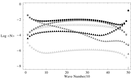
Figure 2: Spectrum of created particles on a lattice that begins with 999 points and ends with 1001 points after a birth process as depicted in Fig. 1. Plotted is the Log of the mean number of left-moving particles vs. $n/10$, where the wave number is $k=2\pi n/1001$. Black squares give the total, while the other curves show the contributions from the left- and right-movers (grey and unfilled squares), the symmetric and anti-symmetric birth modes (grey and black triangles), and the zero-mode (unfilled triangles). The zero-mode parameter is $\gamma=0.4$.

The spectrum of left-moving created particles is displayed in Fig. 2, along with the contributions to the mean number (50) from the left-movers, right-movers, zero-mode, symmetric birth mode, and anti-symmetric birth mode. The number of lattice points starts out as $999$, and the zero-mode parameter $\gamma=0.4$ in (39) has been chosen. Most of the contribution comes from the symmetric birth mode at low wavenumbers, from the anti-symmetric birth mode at high wave numbers, and from the harmonic modes at intermediate wave numbers. The contribution from left-moving harmonic modes is several times higher than from right-moving ones except at very low and very high wave numbers. The contribution from the zero-mode is far smaller than all the rest.

The number itself is presumably not as relevant as the energy of the created particles. As discussed in section 5.2.3, the Hamiltonian—and therefore the energy—is not well-defined on a lattice, due to the ambiguity of adding any multiple of $2\pi/\epsilon$ to eigenvalues of the Hamiltonian without altering the evolution operator. Nevertheless, we presume that, as a model for the microstructure of spacetime, the degree of excitation relative to the translation-invariant Fock vacuum is relevant in determining the gravitational back-reaction. We further presume that the smallest positive value of the frequency for a given positive-norm mode would determine its gravitating energy, at least for modes with frequency much less than $2\pi/\epsilon$ (mod $2\pi/\epsilon$).

This energy and its $N$ dependence can be understood roughly from the form of the Bogoliubov coefficients in the appendix as follows. The squared Bogoliubov coefficients (53,54) for harmonic in- and out-modes (38) goes as $|\beta_{kl}|^{2}\sim N^{-2}(\sin k/\sin l)$. The sum over $l$ values gives $\sum_{l}(1/\sin l)=O(N\ln N)$, so the contribution to the number from harmonic modes goes as $(\ln N/N)\sin k$. A given $k$ mode carries an energy $k$. (Possibly we should instead use $\sin k$, but that difference will not qualitatively affect the result.) Multiplying the number by $k$ and summing over $k$ values yields $\sum k\sin k=O(N)$, hence the total energy contribution from the harmonic in-mode terms is $O(\ln N)$.

For the symmetric birth mode the Bogoliubov coefficient goes as $|\beta_{kS}|^{2}\sim(N\sin k)^{-1}$ as long as $k$ is not too close to $\pi$. Multiplying by the energy $k$ then yields the sum $\sum_{k}(k/\sin k)=O(N)$, hence the contribution to the energy is $O(1)$. A similar result holds for the antisymmetric birth mode, with a suppression from $k$ near zero. The squared zero-mode Bogoliubov coefficient is suppressed by an additional factor of $1/N$, yielding an energy contribution of order $O(\ln N/N)$.

The total created energy due to the birth event is thus of order $\epsilon^{-1}\ln N$, where the dimensionful constant $\epsilon$ setting the scale of length is restored. If every unit of spatial length is born accompanied by this amount of energy creation, the result would be incompatible with the effective field theory notion that the field remains near the adiabatic ground state. A doubling of the size of the universe would produce a Planck energy density of particles in this one-dimensional model.

It is possible as usual to express the out-vacuum $|0_{\rm out}\rangle$ as a squeezed state in the Fock space of the in-modes. If $\alpha_{ki}$ and $\beta_{ki}$ are the Bogoliubov coefficients defined by $a_{k,{\rm out}}=\sum_{i}(\alpha_{ki}a_{i}+\beta_{ki}a_{i}^{\dagger})$, this state takes the form $\exp(-\alpha^{-1}_{ik}\beta_{kj}a_{i}^{\dagger}a_{j}^{\dagger})|0_{\rm in}\rangle$, where repeated indices are summed. In this squeezed state the in-modes are excited and there are specific correlations between the excitations of the different in-modes.

If the ingoing harmonic modes are assumed to be in their ground state, however, no amount of fiddling with the birth mode states and the correlations between those and the harmonic modes can substantially change the amount of energy created. The out-annihilation operator can be expanded as

$$a_{k,{\rm out}}=\alpha_{kl}a_{l,{\rm in}}+\beta_{kl}a^{\dagger}_{l,{\rm in}}+\alpha_{kB}a_{B}+\beta_{kB}a^{\dagger}_{B},$$ (51)

where both birth modes are lumped into the one index $B$. Assuming only that the in-state is the vacuum for the harmonic (and zero-) modes, $a_{l,{\rm in}}|0\rangle=0$, the mean number evaluates to

$$\langle 0_{\rm in}|N_{k,{\rm out}}|0_{\rm in}\rangle=\sum_{l}|\beta_{kl}|^{2}+\|(\alpha_{kB}a_{B}+\beta_{kB}a^{\dagger}_{B})|0\rangle\|^{2}.$$ (52)

The birth mode state could be chosen so that the second term in (52) vanishes, but this would not have a substantial impact on the order of magnitude of the injected energy. The spectrum in Fig. 2 shows that, by themselves, the harmonic modes already contribute an order unity fraction.

Without modifying the assumption that there are no incoming particles, the only way to change this conclusion is to modify the evolution rule. This rule affects the in-Fock representation, so it affects the state corresponding to the in-Fock vacuum. The expectation value of the out-number-operator (52) is sensitive to this via the Bogoliubov coefficients $\beta_{ki}=\langle\chi_{k},\bar{\xi}_{l}\rangle$, since the out-modes $\chi_{k}$ are not defined until the birth time. Some of these coefficients can be suppressed by adjusting the evolution rule. One could tune the rule to kill individual coefficients, or one could choose a “smoothing” interpolation rule that would suppress the contributions from low wave numbers. However, it seems clear that there is no way to avoid the $O(\epsilon^{-1})$ energy injection.

7 Discussion

Using the notion of a phase space of half-solutions, we have managed to quantize a linear field theory on the background of a lattice with a growing number of points. To ensure a well defined symplectic structure on a linear phase space the lattice was assumed to be layered by time slices, and to admit at most one backwards evolution, and at least one forward evolution from any initial data. We were forced to this rather special structure by the requirement of staying very close to standard linear QFT. It may be possible to generalize the structure in various ways and still make sense of the quantum theory. One obvious small generalization would be to a different type of lattice that is still layered.

The computation of particle creation in the two-dimensional model showed that the addition of two points necessarily injects an energy of order $\epsilon^{-1}$ into the field. If more points are added at different times, a similar energy is injected for every unit of length $\epsilon$ added. Since the in-state is no longer the in-vacuum, the particle production would not be identical, but it must clearly be of the same order of magnitude. This would produce an enormous energy density of order $\epsilon^{-2}$ during expansion of a model two-dimensional universe. Extrapolating to our four-dimensional universe, this behavior is not observed. One might hope that in four dimensions the effect of adding points at the lattice scale would not be so brutal, but this seems highly unlikely, as the form of the Bogoliubov coefficients should be comparable to those in the appendix. This should be expected, since the birth process violates time and space translation symmetry on a time and length scale of $\epsilon$, hence it it should be accompanied by a violation of energy conservation of order $\epsilon^{-1}$.

A way out of this energy catastrophe might arise if many points are added at the same time. Then many modes are born at the same time, and wave interference could perhaps suppress the net energy injected. This question can be studied in the two-dimensional model.

If interference effects cannot reduce the injected energy, then one would conclude that QFT on a background growing lattice is not the right setting to describe mode birth in a growing universe. If there is nevertheless a physically correct formulation, it would presumably operate at the level where the spacetime itself is treated as dynamical, rather than as a fixed background. The complete dynamics might ensure that the system remains near the adiabatic vacuum. Perhaps this scenario could be explored using the causal dynamical triangulations formulation of quantum gravity[14].

Apart from trying to address the fundamental problem of the cosmological vacuum, our formulation of mode birth could be applied to field propagation outside a black hole. In a geodesic normal coordinate system the spatial metric grows with respect to the geodesic proper time, by an amount that depends upon the radius. Discretizing the radial coordinate and keeping time continuous one obtains an expanding lattice version of the black hole spacetime in which the number of degrees of freedom is constant. The Hawking effect on such a falling spatial lattice was studied in [15, 16]. It was found that the outgoing modes arise via a process analogous to Bloch oscillation, and the continuum Hawking effect is recovered when the lattice spacing is small compared to the inverse surface gravity of the horizon. Rather than keeping time continuous and allowing the lattice to expand, one could instead discretize the time and allow for points to be added so as to keep the lattice scale roughly constant. This would bring into play the sort of indeterminate evolution and mode birth studied here. In spite of the energy injection by mode birth, the Hawking effect could presumably be recovered provided the Hawking occupation number per outgoing mode is greater than the number induced by the birth events.

Appendix A Bogoliubov coefficients

In this appendix we present the inner-products between harmonic out-modes and the various negative-norm in-modes that appear in the two-dimensional, growing lattice example of Section 6.

For our purposes—calculation of the value of the number operator—we need only the norm of the value of the inner products. Consequently, we can freely choose the over-all phase of a given mode. For definiteness, here we set the phase of the out-modes to zero at point $d$ (see Figure 1 for point labels). For the harmonic, non-zero in-modes, we have set the phase to zero at point $h$. The left-moving mode, when evolved according to the rule of Section 6.3.1, has zero phase at point $d$, the left child of $h$. The right-moving mode has zero phase at point $g$, the right child of $h$. We take the zero-mode and the birth modes exactly as defined in Section 6.3.2.

The formulas correspond to a left-moving harmonic out-mode $\chi_{k}$ (we do not consider the out-zero-mode). The results for a right-moving mode are identical up to a phase, except that Eqn. (53) now corresponds to the inner product with a right-moving in-mode, and Eqn. (54) to that with a left-moving in-mode. All formulas hold for either sign of $k$; i.e. for both positive- and negative-norm out-modes. The positive-norm modes correspond to those for which $\sin(k)>0$, and vice-versa for the negative-norm modes.

For the inner-product with a left-moving in-mode of wave-number $l$, $\xi_{l}^{L}$, we have:

$$\begin{split}\langle\xi^{L}_{l},\chi_{k}\rangle&=A_{N-2}^{l}A_{N}^{k}\sin{k}\Bigl{(}e^{i(l-k)}+\sum^{N-3}_{n=0}e^{in(l-k)}\Bigr{)}\\ &=A_{N-2}^{l}A_{N}^{k}\sin k\Bigl{(}e^{i(l-k)}+\frac{1-e^{i(N-2)(l-k)}}{1-e^{i(l-k)}}\Bigr{)},\end{split}$$ (53)

with $A_{N}^{k}=1/\sqrt{N|\sin{k}|}$. For a right-moving in-mode with wave-number $l$, $\xi_{l}^{R}$, we have:

$$\langle\xi^{R}_{l},\chi_{k}\rangle=-e^{i(l-2k)}A_{N-2}^{l}A_{N}^{k}\sin{k}.$$ (54)

The above hold for both positive- and negative-norm in-modes, which one can classify by the sign of sine of the wave-number.

For the negative-norm in-zero-mode, $\xi_{0}^{-}$, with free-parameter $\gamma$, we have:

$$\langle\bar{\xi}_{0}^{(\gamma)},\chi_{k}\rangle=e^{-i2k}\Bigl{(}\frac{A_{N}^{k}}{\sqrt{2\gamma(N-2)}}\Bigr{)}\bigl{(}(-1+i\gamma)\sin k+2\gamma e^{ik/2}\cos\tfrac{k}{2}\bigr{)}.$$ (55)

For the negative-norm, symmetric birth mode $\bar{S}$, we have:

$$\langle\bar{S},\chi_{k}\rangle=e^{-i2k}\Bigl{(}\frac{A_{N}^{k}}{\sqrt{2}}\Bigr{)}\bigl{(}2i\cos^{2}(k/2)-e^{ik/2}\cos(k/2)\bigr{)}.$$ (56)

For the negative-norm, anti-symmetric birth mode $\bar{A}$, we have:

$$\langle\bar{A},\chi_{k}\rangle=e^{-i2k}\Bigl{(}\frac{A_{N}^{k}}{\sqrt{2}}\Bigr{)}\bigl{(}\sin k+ie^{ik/2}\sin(k/2)\bigr{)}.$$ (57)

To obtain the inner-products with the positive-norm birth or zero-modes, one can use the fact that, from the definition of the inner-product, $\langle\phi,\psi\rangle=-\langle\phi^{*},\psi^{*}\rangle^{*}$, where * denotes complex conjugation. For example, $\langle S,\chi_{k}\rangle=-\langle\bar{S},\chi_{-k}\rangle^{*}$.

References

- [1] T. Jacobson, Trans-Planckian redshifts and the substance of the space-time river, Prog. Theor. Phys. Suppl. 136 (1999) 1 [hep-th/0001085].
- [2] L. Bombelli, J. H. Lee, D. Meyer and R. Sorkin, Space-Time As A Causal Set, Phys. Rev. Lett. 59 (1987) 521.
- [3] R. D. Sorkin, Causal sets: Discrete gravity (Notes for the Valdivia Summer School), [gr-qc/0309009].
- [4] A. R. Daughton, The Recovery of locality for casual sets and related topics, UMI-94-01667 (Ph.D. Thesis, Syracuse University, 1993).
- [5] R. F. Blute, I. T. Ivanov and P. Panangaden, Decoherent histories on graphs, [gr-qc/0111020].
- [6] R. F. Blute, I. T. Ivanov and P. Panangaden, Discrete quantum causal dynamics, Int. J. Theor. Phys. 42 (2003) 2025 [gr-qc/0109053].
- [7] E. Hawkins, F. Markopoulou and H. Sahlmann, Evolution in quantum causal histories, Class. and Quant. Grav. 20 (2003) 3839 [hep-th/0302111].
- [8] R. Haag, Local Quantum Physics: Fields, Particles, Algebras, (Springer-Verlag, 1992).
- [9] R. M. Wald, Quantum Field Theory In Curved Space-Time And Black Hole Thermodynamics, (The University of Chicago Press, Chicago, 1994).
- [10] A. Kempf, Mode generating mechanism in inflation with cutoff, Phys. Rev. D 63 (2001) 083514 [astro-ph/0009209].
- [11] N. Sasakura, Field theory on evolving fuzzy two-sphere, Class. and Quant. Grav. 21 (2004) 3593 [hep-th/0401079].
- [12] D. R. Finkelstein, H. Saller and Z. Tang, Beneath gauge, Class. and Quant. Grav. 14 (1997) A127 [quant-ph/9608023]; Hypercrystalline vacua, [quant-ph/9608024].
- [13] F. D. Smith, Hyperdiamond Feynman checkerboard in four-dimensional space-time, [quant-ph/9503015].
- [14] J. Ambjorn, J. Jurkiewicz and R. Loll, A non-perturbative Lorentzian path integral for gravity, Phys. Rev. Lett. 85 (2000) 924 [hep-th/0002050]; Dynamically triangulating Lorentzian quantum gravity, Nucl. Phys. B 610 (2001) 347 [hep-th/0105267]; Non-perturbative 3d Lorentzian quantum gravity, Phys. Rev. D 64 (2001) 044011 [hep-th/0011276]; Emergence of a 4D world from causal quantum gravity, [hep-th/0404156].
- [15] S. Corley and T. Jacobson, Lattice black holes, Phys. Rev. D 57 (1998) 6269 [hep-th/9709166].
- [16] T. Jacobson and D. Mattingly, Hawking radiation on a falling lattice, Phys. Rev. D 61 (2000) 024017 [hep-th/9908099].