Supersymmetric solutions of supergravity from wrapped branes

Ángel Paredes

Departamento de Física de Partículas, Universidade de Santiago de Compostela

E-15782 Santiago de Compostela, Spain

angel@fpaxp1.usc.es

ABSTRACT

We consider several solutions of supergravity with reduced supersymmetry which are related to wrapped branes, and elaborate on their geometrical and physical interpretation. The Killing spinors are computed for each configuration. In particular, all the known metrics on the conifold and all $G_{2}$ holonomy metrics with cohomogeneity one and $S^{3}\times S^{3}$ principal orbits are constructed from D=8 gauged supergravity in a unified formalism. The addition of 4-form fluxes piercing the unwrapped directions is also considered. We also study the problem of finding kappa-symmetric D5-probes in the so-called Maldacena-Núñez model. Some of these solutions are related to the addition of flavor to the dual gauge theory. We match our results with some known features of ${\cal N}=1$ SQCD with a small number of flavors and compute its meson mass spectrum. Moreover, the gravity solution dual to three dimensional ${\cal N}=1$ gauge theory, solutions related to branes wrapping hyperbolic spaces, $Spin(7)$ holonomy metrics and $SO(4)$ twistings in D=7 gauged sugra are studied in the last chapter.

hep-th/0407013

What Immortal hand or eye

Dare frame thy fearful symmetry?

William Blake, “The Tyger”.

Motivation

There are four kinds of interactions known to exist in nature: gravitational, electromagnetic, weak and strong. The first one, much weaker than the rest, is described by Einstein’s General Theory of Relativity. The other three are accurately explained by the successful Standard Model, based on quantum gauge theories. Unfortunately, it is known that both theories are incompatible at very small distances or very high energy scales, of the order of the Planck mass, about $10^{19}$ GeV. This means that some new physics must happen when approaching the Planck scale.

Superstring theory, despite being originally formulated as an attempt to explain strong interactions, is, nowadays, the most promising candidate for solving this puzzle. Its basic idea is to suppose that particles, instead of being points, have some natural extension and are, in fact, vibrational modes of some fundamental strings.

By studying the spectrum of excitations of a closed string, one finds a massless spin-two field, which can be identified with the graviton. On the other hand, the infinite tower of massive string modes can cure the non-renormalizability of General Relativity, thus yielding a consistent theory of quantum gravity. Since the eighties, lots of theoretical physicists have hoped that string theory can lead to a “Theory of Everything”, that should describe consistently all the measured phenomena. Standard texts on string theory are [1].

The fact that five consistent string theories can be formulated was a puzzle: how should nature choose one among several possibilities? This question was nicely solved when the existence of a web of dualities relating all of them was discovered. The so-called M-theory lives in eleven dimensions and the different string theories are different perturbative regimes. Besides, eleven dimensional supergravity also appears as a low energy limit.

The objects called branes play an important rôle in this picture. D-branes are non-perturbative solitonic objects that can be identified with hyperplanes where open strings can end (an introduction on branes can be found in [2]). The dynamics of the D-branes can be described by the physics of the open strings, thus giving rise to a gauge theory living on the worldvolume of the brane (see [3] for a review of the interplay between brane dynamics and gauge theory). However, there is another way of thinking about D-branes, as sources of closed strings. From this point of view, branes are objects that modify the gravitational background, i.e. the geometry of space-time. Therefore, this open/closed string duality leads to a gauge/gravity duality. This notion has opened new and amazing possibilities. Besides addressing the problem of unification, string theory can give an insight in the search of duals of different gauge theories.

This fact is related to a much older proposal by t’Hooft [4]. He pointed out that the Feynman diagrams of a $U(N)$ gauge theory can be rearranged as a sum over the genus of the surfaces in which the diagrams can be drawn. This is pretty similar to the computation of string amplitudes, where there is a sum over the genus of the possible worldsheets. Then, there is a gauge/string duality, at least in some regime of parameters. The problem is that no hints are given of which should be the string theory that corresponds to each gauge theory.

In 1997, Maldacena formulated an astonishing conjecture along these lines [5]. The statement is that type IIB string theory living on $AdS_{5}\times S^{5}$ is exactly dual to four dimensional ${\cal N}=4$ super Yang-Mills theory with $SU(N)$ gauge group (which is called AdS/CFT duality since the gauge theory is conformal). Although a strict proof has not been given, the duality has overcome a large number of tests (the standard review on these topics is [6]). The duality between two such different theories was reached by looking at the dual open/closed string descriptions of the near horizon limit of a stack of $N$ D3-branes. The low energy limit of string theory yields a supergravity theory, and we find that type IIB sugra on $AdS_{5}\times S^{5}$ is dual to ${\cal N}=4$ SYM in its non-perturbative regime.

A remarkable fact is that the relation between the two theories that are supposed to be equivalent is holographic [7]. This means that the number of dimensions in which they live is different and, that, somehow, the physics on the boundary of a space encodes all the bulk information.

Following these ideas, a lot of work has been devoted to the research on other possible dualities involving more realistic gauge theories. In particular, one would like to have less supersymmetry and break conformal invariance. The final goal is to find a gravity dual of QCD, at least for the limit with large number of colors.

The motivation of this work is this amazing interplay between strings, gravity, geometry and gauge theory. When branes are wrapped, the amount of supersymmetry of the solution gets reduced and, in fact, conformal symmetry gets broken. However, in order to have some supersymmetry, the branes must be wrapped along certain supersymmetric cycles which are embedded in non-trivial spaces. With these ingredients, one can engineer several setups, such that different gauge theories live on the worldvolume of the wrapped branes. Supergravity techniques will be used in order to get geometrical results about these spaces with reduced supersymmetry, and also to obtain features of the dual gauge theories.

About this thesis

This Ph.D. thesis is mainly based on papers [8, 9, 10, 11], although a few unpublished results are also discussed. Throughout the work, technical details are described thoroughly at many points (mainly the way of obtaining and solving BPS systems of equations). However, sometimes it is possible to skip them while keeping a comprehensive reading of the text. The plan for the rest of the thesis is the following:

In chapter 1, there is a brief introduction to the ideas of supersymmetry and supergravity. Then, some general strategies for computing supersymmetric solutions of supergravity are presented. Finally, the degrees of freedom, lagrangians and susy transformations of several supergravity theories are reviewed. This chapter provides the basic prerequisites needed and sets up the notation for the computations of the following.

In chapter 2, we use eight-dimensional supergravity to study the geometry of the so-called conifold. The metric and Killing spinors are found. In the process, we will find an important technical point: the need of having a rotated projection on the spinor. In chapter 3, 8d sugra is used again, this time for computing metrics of seven-dimensional $G_{2}$ holonomy manifolds. Assuming again a rotated Killing spinor, all the complete metrics of cohomogeneity one and $G_{2}$ holonomy with $S^{3}\times S^{3}$ principal orbits are constructed. It will be shown how asymptotically locally conical metrics are obtained from this approach. Then, in chapter 4, we find a general procedure to incorporate RR fluxes in the unwrapped directions of configurations of the type of those mentioned above. From an M-theory point of view, this amounts to adding M2-branes to the solution.

Then, in chapter 5, we turn to the so-called Maldacena-Núñez model. In this scenario, the gravity solution corresponding to D5-branes wrapping a supersymmetric two-cycle inside a Calabi-Yau is dual to ${\cal N}=1$ super Yang-Mills theory in four dimensions. A brief review of the model is presented and the supergravity solution is computed from an analysis of supersymmetry. The Killing spinors are obtained in the process. In chapter 6, we address a concrete problem within this model. We look for surfaces where supersymmetric brane probes can be placed. We argue that some of these brane probes introduce fundamental quarks in the dual gauge theory, which are represented by fundamental strings stretching from the brane probe to the gauge theory brane. Some known features of the ${\cal N}=1$ gauge theory are recovered from the gravity viewpoint and a prediction is made about the meson mass spectrum.

Finally, in chapter 7, the supersymmetry of a few more supergravity solutions is studied.

Chapter 1 Some notes on supergravity

The main goal of this thesis is to find (bosonic) supersymmetric configurations which are solutions of some supergravity equations of motion, and to deepen in their physical and geometrical interpretation. This chapter is aimed to be the basis of the analysis carried out in the rest of this work.

First of all, a brief (and surely incomplete) introduction to what is supergravity will be given. Then, the general strategy that will be used to find the different solutions will be established. After that, several supergravities that will appear throughout the rest of the thesis, and the relation between them, will be presented. This is useful to fix notation for the following chapters. Notice that some of the actions and supersymmetry transformations written here are not the most general ones, but only truncations where some fields have been set to zero. An important concept for finding supersymmetric solutions in gauged supergravities is the twisting (which amounts to exciting the gauge field). It will be introduced in section 1.5.

1.1 What is Supersymmetry?

Supersymmetry (susy) can be defined as a Fermi-Bose symmetry, i.e. as a transformation mixing bosonic and fermionic degrees of freedom which leaves the physics (the equations of motion) invariant.

It was first discovered by studying the interplay between the space-time Poincaré symmetry (Lorentz group plus translations) and internal symmetry groups. A theorem by Coleman and Mandula stated that if both Poincaré and internal symmetry are present (subject to a few hypothesis), they do not have non-trivial mixing, i.e., the full symmetry group should be a direct product of both.

One of the hypothesis was that the internal symmetry was described by a Lie group based on commutators, but it was realized in the seventies that the no-go theorem could be avoided by taking a Lie algebra based on anticommutators.

The supersymmetry algebra can be written in a completely schematic fashion (for a rigorous discussion, see, for example, [12]):

$$[P,P]=0;\qquad\quad\quad\,\,[P,M]=P;$$

$$[M,M]=M;\qquad\,\quad[P,Q^{I}]=0;$$

$$[M,Q^{I}]=Q^{I};\ \ \quad\quad\,\{Q^{I},\bar{Q}^{J}\}=P\,\delta^{IJ};$$

$$\{Q^{I},Q^{J}\}=Z^{IJ};\ \,\quad\,\{\bar{Q}^{I},\bar{Q}^{J}\}=Z^{IJ};$$ (1.1.1)

where the $P$ stands for translations, $M$ for Lorentz generators (spatial rotations and boosts), $Q^{I}$, $\bar{Q}^{I}$ for the supersymmetry generators, and $Z^{IJ}$ are the central charges. All space-time and spinor indices have been omitted. The indices $I,J=1,...,\cal N$ label different sets of supersymmetry generators.

For consistency, the supersymmetry generators must transform as 1/2 spinors under Lorentz transformations (this fact could have been intuitively anticipated because their algebra is based on anticommutators). This has the immediate consequence that under a susy transformation, bosons turn into fermions and vice versa. So an irreducible representation of the susy algebra will correspond to several particles, forming what is called a supermultiplet. It can be proved that a supermultiplet always contains the same number of bosonic and fermionic degrees of freedom. Furthermore, as susy transformations commute with momemtum generators, we have, in particular $[P^{2},Q]=0$, and therefore all particles in the same supermultiplet have the same mass.

At this point, one may think that, although possibly interesting from a theoretical point of view, supersymmetry could be far from reality because, if there were supersymmetric particles with the same mass as the usual ones, they would have been certainly observed by now. The only way out to this problem is to say that, if supersymmetry exists, it must be broken at a scale of energy at least as high as the energies probed in accelerators. Anyway, experimentally there is not even a hint on the existence of susy particles, so the next question to answer is: why physicists have been (and still are) so interested in supersymmetry during the last decades?

First of all, supersymmetric theories are the most natural extension of the usual quantum field theories and they have the advantage with respect to them of a better UV behavior because the bosonic and fermionic loops cancel one against each other.

Maybe the fact that gives strongest support to the idea of susy really existing in nature is Grand Unification. If the standard model gauge group comes from the breaking of a larger gauge group at some high mass scale, the three couplings (electromagnetic, weak and strong) should get unified at that scale. Following the renormalization group flows using the standard model spectrum of particles, the couplings fail to converge at a point. But using a supersymmetric extension of the model, this problem can be overcome. Another argument in favor of susy is based on the hierarchy problem. The big difference between the Planck scale and the electroweak scale suggests that susy should be restored at a scale comparable to the Higgs mass. A third physical puzzle which may be solved by the existence of supersymmetric particles is the dark matter. The WIMPS (weakly interacting massive particles) that are thought to form it, could be some of the yet unobserved superpartners. All these three arguments tend to signal to the same value for the mass of the lightest susy particles: about a few TeV. If this is true, the Large Hadron Collider which will be soon operative at CERN should confirm the existence of superpartners.

Yet another reason to believe in supersymmetry is that it appears in a very natural way in string theory, and it is required to keep the theory free of tachyons (and therefore inconsistencies).

Even if susy turned out not to be real, it would continue to be quite interesting for some reasons. Susy theories are in general simpler than non-susy ones because of the constraints imposed by the symmetry. Then, they can be used as toy models that could hopefully capture features of more realistic theories and help to understand difficult problems like confinement. Susy can also give an insight into mathematical problems (specially, in geometry) as it will become clear in the following chapters, and has led to great developments like mirror symmetry. And finally, even if superstring theories are not the correct description of quantum gravity, they would still have a major physical interest because of the gauge/string duality, that can be explored along the lines of Maldacena’s conjecture.

Spinors in arbitrary dimensions

As in the following we will deal with supersymmetric theories in different number of dimensions, it is convenient to take a brief look at spinor representations in any number of dimensions. For a nice review on this topic, see [13].

A spinor representation of the Lorentz group is associated to a Clifford algebra:

$$\{\Gamma_{\mu},\Gamma_{\nu}\}=2\;g_{\mu\nu}\,\,,$$ (1.1.2)

where $\mu,\nu=1,...,D$ are space-time indices (and so $D$ is the dimension of space-time). It can be proved that, in order to have a representation of this algebra, the Dirac gamma matrices can be written as $2^{[D/2]}\times 2^{[D/2]}$ complex square matrices ($[D/2]$ being the integer part of $D/2$). Then, a spinor has $2^{[D/2]}$ complex components, whose degrees of freedom are halved because they must satisfy the Dirac equation. In conclusion, a Dirac spinor in $D$ dimensions has $2^{[D/2]}$ real degrees of freedom (but notice that this halving does not apply for the spinors used for the susy transformations, as they are arbitrary and do not need to satisfy any equation of motion). Furthermore, it is important to know whether it is possible to impose some condition that consistently reduces the number of degrees of freedom of the spinor, as it turns out that supergravity multiplets are constructed in each dimension with these reduced spinors.

There are two types of such conditions. Each of them halves the number of degrees of freedom:

• Imposing reality of the spinors gives rise to the so-called (pseudo) Majorana spinors. This can be done when $D$=0,1,2,3,4 mod 8 (assuming that there is just one time-like dimension).

• Imposing that the spinors have a definite chirality gives rise to the so-called Weyl spinors. This is possible when the dimension of space-time is even.

• Both conditions can be imposed simultaneously when $D$=2 mod 8, getting (pseudo) Majorana-Weyl spinors.

This is useful to know how many supercharges there exist in a susy theory. For example, in an ${\cal N}=1$, $D=11$ theory, the supersymmetry is generated by one Majorana spinor that has 32 degrees of freedom and therefore there are 32 associated real supercharges, while in an ${\cal N}=1$, $D=4$ theory, there are only 4 supercharges.

1.2 What is Supergravity?

Supergravity (sugra) is the gauge theory of supersymmetry.

The basic idea is to formulate a supersymmetric theory including Einstein’s general relativity. General relativity is a theory whose basic field is a spin 2 particle, the graviton. The supermultiplet of the graviton must, at least, contain a spin 3/2 particle (a Rarita-Schwinger field), the so-called gravitino. In general relativity, there is a gauge symmetry that consists in reparametrizations of space-time, which are generated by the momentum operator. As supersymmetry transformations are related to the momentum operator in eq. (1.1.1), we conclude that they must also be local.

This fact is quite restrictive for the construction of supergravity theories. In particular, the maximum number of dimensions where a consistent supergravity can be formulated is $D=11$ with ${\cal N}=1$. In dimensions lower than 11, a bunch of supergravities have been constructed in the last decades. Most of them are obtainable by Kaluza-Klein reducing the $D=11$ sugra in some compact space. A set of new fields will always appear upon dimensional reduction, as space-time indices along the directions where compactification has been performed turn into internal indices. If one knows the compactification ansatz that relates two supergravities of different dimension, a solution of one of them can be easily reduced (or uplifted) to the other one (provided the solution somehow respects the symmetries of the compact space). This procedure is quite useful in the search of solutions, as will become clear in the following chapters.

Historically, supergravity was born as a good candidate to solve the problem of unifying gravity with the rest of interactions. The boson-fermion loop cancellation was expected to cure the non-renormalizability of gravity, while the gauge fields and interactions could come from the Kaluza-Klein reduction. Today, it is apparent that this is not the whole story. String/M-theory is now the main candidate for unification. However, supergravities appear as low energy limits of string theories (when the massive string oscillations have been frozen). In particular, $D=11$ supergravity is the low energy limit of M-theory (it cannot be a coincidence when the maximal supergravity lives in the same number of dimensions as the postulated “Theory of Everything”!).

1.3 Looking for Supersymmetric Solutions: General Strategies

The aim of this section is to describe the methods that will be later used in the search of sugra solutions. The problem in finding solutions is that the supergravity equations of motion are, in general, complicated systems of second order equations. The idea is to find somehow, systems of first order equations (much simpler to deal with), which automatically solve the second order problem. Supersymmetric solutions will always satisfy such a first order system (of course, there exist non-susy solutions that cannot be found following these strategies).

Another notion we should keep in mind is the possibility of uplifting a solution obtained in a low dimensional sugra to ten or eleven dimensions where its physical interpretation is clearer. We will use gauged supergravity theories that can be formulated by compactifying another supergravity in higher dimension. In section 1.4, some expressions that facilitate the task of finding the high dimensional solutions from the low dimensional ones can be found.

1.3.1 Vanishing of fermion field variations

We will look for classical configurations, so the expectation value of the fermionic fields should be zero. As explained in section 1.1, supercharges are spin 1/2 fields and they turn fermions into bosons and vice versa. Schematically:

$$\delta F = f(B)\,\,,$$ (1.3.1)

$$\delta B = g(F)\,\,,$$ (1.3.2)

where $f(B)$ and $g(B)$ are some functions of the bosonic and fermionic fields respectively and $\delta$ means susy transformation. As the fermions are zero ($\Rightarrow g(F)=0$), the invariance of the bosonic fields describing the solutions is guaranteed. In order to preserve susy, the fermionic fields should also not vary, hence:

$$f(B)\,=\,0\,\,,$$ (1.3.3)

which gives the desired system of equations, first order in derivatives.

There are some points worth to comment about this:

The only way of having a manageable system of equations is to start with an ansatz for the bosonic fields. Then, (1.3.3) leads to a system from which the functions in the ansatz can be computed. Needless to say that, to find interesting solutions, it is a requisite to begin with the correct ansatz.

That a configuration is supersymmetric does not necessarily imply that it is a solution of the supergravity equations of motion. However, as susy configurations are related to BPS states, which saturate some energy bound, they usually are, actually, solutions of the sugra equations of motion. Anyway, the correct way of proceeding is to first find the configurations by imposing supersymmetry and then to directly check the second order equations of motion.

Usually, for eqs. (1.3.3) to be solvable, one must impose some projections on the spinor that parameterizes the transformation. When this happens, not all the supercharges present in the supergravity theory are preserved by the solution. These projections are of the type $P\epsilon=\epsilon$ ($P$ being some function of the gamma matrices, which will be explicitly showed for each solution. Notice that all the projectors should commute among themselves). An important point is that each independent projection halves the number of preserved supercharges.

1.3.2 Superpotential method

By plugging an ansatz for the fields in terms of some functions $\alpha^{i}$ depending on a single coordinate $\eta$ (which in all the cases studied in this work will be a radial coordinate), one gets a one-dimensional action. If the action satisfies certain conditions, there is a direct way of getting a first-order system which solves the equations of motion.

Let us consider a lagrangian of the type ($S=\int L\,d\eta$):

$$L\,=\,\frac{1}{2}\,g_{ij}\,\frac{d\alpha^{i}}{d\eta}\,\frac{d\alpha^{j}}{d\eta}\,-\,V\,\,,$$ (1.3.4)

where $g_{ij}$ is a symmetric matrix (that might depend on the functions $\alpha^{i}$) and $V\equiv V(\alpha^{i})$. The second order Euler-Lagrange equations are:

$$\frac{d}{d\eta}\left[g_{ij}\frac{d\alpha^{j}}{d\eta}\right]\,=\,\frac{1}{2}\left(\frac{\partial}{\partial\alpha^{i}}\,g_{jk}\right)\frac{d\alpha^{j}}{d\eta}\frac{d\alpha^{k}}{d\eta}-\frac{\partial V}{\partial\alpha^{i}}\,\,.$$ (1.3.5)

Let us assume that the potential can be written as:

$$V=-\,\frac{1}{2}\,g^{ij}\,\frac{\partial W}{\partial\alpha^{i}}\frac{\partial W}{\partial\alpha^{j}}\,\,,$$ (1.3.6)

for some function $W(\alpha^{i})$, which we will call superpotential, and where $g^{ij}$ has been defined as the inverse of $g_{ij}$: $g_{ij}g^{jk}=\delta_{i}^{\ k}$. Then, it can be straightforwardly proved that the first order system:

$$\frac{d\alpha^{i}}{d\eta}\,=\,\mp\,g^{ij}\frac{\partial W}{\partial\alpha^{j}}\,\,,$$ (1.3.7)

automatically solves (1.3.5). Moreover, on this solution of the equations of motion, the hamiltonian identically vanishes:

$$H\,=\,\frac{\partial\alpha^{i}}{\partial\eta}\frac{\partial L}{\partial\frac{d\alpha^{i}}{d\eta}}\,-\,L\,=\,0\,\,.$$ (1.3.8)

Conversely, it can be proved that any classical system whose hamiltonian does not explicitly depend on time, and whose energy is zero, can be solved this way. In order to prove this assertion, let us use Hamilton-Jacobi’s formalism. The Hamilton-Jacobi equation reads:

$${\partial S\over\partial t}\,+\,H\left(\alpha_{i}\,,{\partial S\over\partial\alpha_{i}}\right)\,=\,0\,\,,$$ (1.3.9)

where the non-explicit dependence of $H$ on $t$ has been taken into account. The Hamilton’s principal function $S$ is the generating function of a canonical transformation to a system where coordinates and momenta are constant. The solution to (1.3.9) is $S=-Et+W(\alpha_{i})$, where the constant $E$ is the energy and $W$ is Hamilton’s characteristic function. The equations of motion written in terms of $W$ are $p_{i}={\partial W\over\partial\alpha^{i}}$, the equivalent of (1.3.7). Moreover, by using (1.3.9), the energy can be written:

$$E=-{\partial S\over\partial t}=H=\frac{1}{2}\,g_{ij}\,\frac{d\alpha^{i}}{d\eta}\,\frac{d\alpha^{j}}{d\eta}\,+V={1\over 2}g^{ij}p_{i}\,p_{j}+V={1\over 2}g^{ij}\frac{\partial W}{\partial\alpha^{i}}\frac{\partial W}{\partial\alpha^{j}}+V\,\,.$$ (1.3.10)

Now, if $E=0$, eq. (1.3.6) is obtained from eq. (1.3.10). This reasoning shows that the function $W$ which has been called superpotential is nothing else than Hamilton’s characteristic function.

A supersymmetric configuration can always be obtained as the solution of a first order system, so this construction is somehow related to supersymmetry in some cases, although by no means it is a proof of it.

It will be useful to apply this method to lagrangians of the type:

$$L\,=\,e^{c_{1}A}\left[c_{2}\,(\partial_{\eta}A)^{2}\,-\,\frac{1}{2}\,G_{ab}(\varphi)\,\partial_{\eta}\varphi^{a}\,\partial_{\eta}\varphi^{b}\,-\,\tilde{V}(\varphi)\right]\,\,,$$ (1.3.11)

where the fields $\alpha^{i}(\eta)$ have been split $\alpha^{i}=(A,\varphi^{a})$, and $c_{1}$ and $c_{2}$ are numbers. This is of the form (1.3.4) with the identifications:

$$g_{AA}=2\,c_{2}\,e^{c_{1}A},\,\,\,\,\,\,\,\,\,\,\,\,\,\,\,\,g_{ab}=-e^{c_{1}A}\,G_{ab},\,\,\,\,\,\,\,\,\,\,\,\,\,\,\,\,V=e^{c_{1}A}\,\tilde{V}(\varphi)\,\,.$$ (1.3.12)

Suppose it is possible to find a function $\tilde{W}(\varphi)$ such that:

$$\tilde{V}(\varphi)\,=\,{c_{3}^{2}\over 2}\,\,G^{ab}\,\frac{\partial\tilde{W}}{\partial\varphi^{a}}\,\frac{\partial\tilde{W}}{\partial\varphi^{b}}\,\,-\,\,{c_{1}^{2}\,c_{3}^{2}\over 4\,c_{2}}\,\tilde{W}^{2}\,\,\,,$$ (1.3.13)

where $c_{3}$ is any constant (notice that it is only an irrelevant rescaling in $\tilde{W}$). Then, equation (1.3.13) is equivalent to (1.3.6) with superpotential:

$$W\,=\,c_{3}\,e^{c_{1}\,A}\,\tilde{W}\,\,.$$ (1.3.14)

And so, equations (1.3.7) read:

$${dA\over d\eta} = \mp\,{c_{1}\,c_{3}\over 2\,c_{2}}\,\tilde{W}(\varphi)\,\,\,,$$ (1.3.15)

$${d\varphi^{a}\over d\eta} = \pm\,c_{3}\,G^{ab}\,{\partial\tilde{W}(\varphi)\over\partial\varphi^{b}}\,\,\,,$$ (1.3.17)

which is the sought system of first-order equations.

Let us summarize all the above reasoning: Having a lagrangian of the form (1.3.11), if one manages to find a function $\tilde{W}(\varphi)$ such that (1.3.13), then the system (1.3.17) solves the equations of motion and, on this solution, condition (1.3.8) holds.

To finish the section, let us make a brief comparison between the two methods presented. The superpotential method is much less straightforward, in the sense that, even if a superpotential (1.3.13) exists, there is no direct way of finding it, and the task may be quite difficult if $\tilde{W}(\varphi)$ is a complicated function. The only problem with the susy variation method is that one has to deal with the Dirac matrices algebra and it may not be simple to find the correct projections that must be imposed on the spinor. But this method has the additional advantage that one finds the amount of supersymmetry preserved and the Killing spinors.

1.4 Supergravity actions and supersymmetry transformations

The aim of this section is to compile the expressions of the different supergravity theories that will be used throughout the thesis. As we will look for bosonic supersymmetric configurations, the only sector of the action we will need is the bosonic one (the configurations must be solution of the Euler-Lagrange equations derived from it). As also explained in the previous section, the supersymmetry transformation of the fermionic fields must be set to zero, so their explicit expression is needed. The relation between supergravities in different number of dimensions is given.

Notice that not all the bosonic fields are excited in the solutions that will be explored, so for the sake of simplicity the fields that will not be used are neglected in the expressions of this section. Anyway, references to the original papers where the full equations can be found will be provided in each subsection.

A note on notation

Both the formalism of differential forms and the formalism where indices are written explicitly will be used. A differential $p$-form is defined as:

$$\omega_{(p)}\,=\,{1\over p!}\omega_{{\mu_{1}}\dots{\mu_{p}}}dx^{\mu_{1}}\wedge\dots\wedge dx^{\mu_{p}}\,\,.$$ (1.4.1)

Here, ${\mu_{1}}\dots{\mu_{p}}$ are curved indices, referred to the coordinate basis. We will often use the tangent space basis, and therefore flat indices:

$$ds^{2}\,=\,g_{\mu\nu}\,dx^{\mu}dx^{\nu}\,=\,\eta_{ab}\,e^{a}e^{b}\,\,,$$ (1.4.2)

where $\eta_{ab}={\rm diag}(-1,+1,\dots,+1)$. The $e^{a}$ one-forms are the components of the so-called vielbein. They can be expressed in components: $e^{a}=e^{a}_{\mu}(x)dx^{\mu}$, so the $e^{a}_{\mu}(x)$ transform between flat and curved indices. The spin connection of a metric can be found by solving the so-called Cartan’s structure equations:

$$0=de^{a}+\omega^{a}_{\ b}\wedge e^{b}\,\,.$$ (1.4.3)

The spin connection is a one-form which in components reads: $\omega^{a}_{\ b}=\omega^{a}_{\ b\mu}dx^{\mu}$. We need to define the covariant derivative, whose action on a spinor is given by:

$$D_{\mu}\epsilon=(\partial_{\mu}+{1\over 4}\,\omega_{\mu}^{ab}\Gamma_{ab})\,\epsilon\,.$$ (1.4.4)

As we will deal with gauged supergravities, we will need at some point to introduce gauge covariant derivatives, i.e. that take into account the gauge connection besides the spin connection. They will be denoted by the symbol ${\cal D}$ and its precise definition will be given in each case.

In (1.4.4), the $\Gamma_{ab}$ are Dirac matrices with indices referring to the vielbein basis. They satisfy the algebra:

$$\{\Gamma_{a},\Gamma_{b}\}\,=\,2\,\eta_{ab}\,\,.$$ (1.4.5)

The symbol with several indices in a single gamma $\Gamma_{\mu_{1}\cdots\mu_{n}}$ will denote an antisymmetrized product of Dirac matrices.

1.4.1 D=11, ${\cal N}=1$ supergravity

Eleven is the maximal dimension where a supergravity can exist [14]. The action and supersymmetry transformation laws were first constructed in [15]. The number of supercharges is 32, corresponding to one Majorana spinor.

The bosonic content of the theory includes only the metric and a 3-form potential (with a 4-form field strength $F_{(4)}=dC_{(3)}$). The action for these fields is:

$${\cal L}=\sqrt{-g}\left[R-\frac{1}{48}F_{\mu\nu\rho\sigma}F^{\mu\nu\rho\sigma}\right]+\frac{1}{144^{2}}\epsilon^{\alpha_{1}\dots\alpha_{4}\beta_{1}\dots\beta_{4}\mu\nu\rho}F_{\alpha_{1}\dots\alpha_{4}}F_{\beta_{1}\dots\beta_{4}}C_{\mu\nu\rho}\,\,.$$ (1.4.6)

The only fermionic degrees of freedom are those corresponding to a Rarita-Schwinger field $\psi_{\mu}$, the gravitino. Its supersymmetry variation is given by:

$$\delta\psi_{\mu}\,=\,D_{\mu}\,\epsilon\,+\,{1\over 288}\,F^{(4)}_{\mu_{1}\dots\mu_{4}}\,\,\Bigg{(}\,\Gamma_{\mu}^{\,\,\mu_{1}\dots\mu_{4}}\,-\,8\,\delta_{\mu}^{\mu_{1}}\,\Gamma^{\,\,\mu_{2}\dots\mu_{4}}\,\Bigg{)}\,\epsilon\,\,,$$ (1.4.7)

1.4.2 D=10 type IIA supergravity

Eleven dimensional supergravity can be dimensionally reduced yielding maximal (i.e. with 32 supercharges) non-chiral supergravity in ten dimensions [16]. The resulting theory is called type IIA supergravity and it is a low energy limit of type IIA string theory. The Kaluza-Klein reduction ansatz for the metric is:

$$ds^{2}_{11}\,=\,e^{-{2\over 3}\,\phi}\,ds^{2}_{10}\,+\,e^{{4\over 3}\,\phi}\,(\,dz\,+\,C_{(1)}\,)^{2}\,\,.$$ (1.4.8)

Furthermore, one has to reduce the eleven dimensional three-form, which generates in ten dimensions a three-form and a two-form, depending on whether or not the reduction direction is comprised among the indices of the original form. Therefore, the bosonic content of this theory consists of a metric $g_{\mu\nu}$, a dilaton $\phi$ and a Ramond-Ramond one-form $C_{(1)}$ coming from the reduction of the metric, besides a Neveu-Schwarz two-form $B_{(2)}$ and an RR three-form $C_{(3)}$ coming from the reduction of the three-form. The bosonic action (in Einstein frame) of this theory is:

$$S = \int d^{10}x\sqrt{-g}\,\left[R-{1\over 2}\partial_{\mu}\phi\,\partial^{\mu}\phi\,-{1\over 12}e^{-\phi}H_{(3)}^{2}-{1\over 4}e^{{3\over 2}\phi}F_{(2)}^{2}-{1\over 48}e^{{1\over 2}\phi}F_{(4)}^{2}\right]+$$ (1.4.9)

$$+\,{1\over 2}\int B_{(2)}\wedge dC_{(3)}\wedge dC_{(3)}\,\,,$$

where the field strengths have been defined: $F_{(2)}=dC_{(1)}$, $H_{(3)}=dB_{(2)}$ and $F_{(4)}=dC_{(3)}+C_{(1)}\wedge H_{(3)}\,$. On the other hand, the fermionic content of the theory comprises two Majorana spinors: a gravitino $\psi_{\mu}$ and a dilatino $\lambda$, each decomposable into two Majorana-Weyl components. Their supersymmetry variations read (Einstein frame):

$$\delta\lambda = {1\over 4}\sqrt{2}\,D_{\mu}\phi\,\Gamma^{\mu}\Gamma^{11}\epsilon+{3\over 16}{1\over\sqrt{2}}\,e^{{3\phi\over 4}}F^{(2)}_{\mu_{1}\mu_{2}}\Gamma^{\mu_{1}\mu_{2}}\epsilon+$$

$$+{1\over 24}{i\over\sqrt{2}}\,e^{-{\phi\over 2}}H^{(3)}_{\mu_{1}\mu_{2}\mu_{3}}\Gamma^{\mu_{1}\mu_{2}\mu_{3}}\epsilon-{1\over 192}{i\over\sqrt{2}}\,e^{{\phi\over 4}}F^{(4)}_{\mu_{1}\mu_{2}\mu_{3}\mu_{4}}\Gamma^{\mu_{1}\mu_{2}\mu_{3}\mu_{4}}\epsilon\,\,,$$

$$\delta\psi_{\mu} = D_{\mu}\epsilon+{1\over 64}\,e^{{3\phi\over 4}}\,F_{\mu_{1}\mu_{2}}^{(2)}\,\left(\Gamma_{\mu}^{\ \mu_{1}\mu_{2}}-14\delta_{\mu}^{\mu_{1}}\Gamma^{\mu_{2}}\right)\Gamma^{11}\,\epsilon\,+$$ (1.4.10)

$$+\,{1\over 96}\,e^{-{\phi\over 2}}\,H_{\mu_{1}\mu_{2}\mu_{3}}^{(3)}\,\left(\Gamma_{\mu}^{\ \mu_{1}\mu_{2}\mu_{3}}-9\delta_{\mu}^{\mu_{1}}\Gamma^{\mu_{2}\mu_{3}}\right)\Gamma^{11}\,\epsilon\,+$$

$$+\,{i\over 256}\,e^{{\phi\over 4}}\,F_{\mu_{1}\mu_{2}\mu_{3}\mu_{4}}^{(4)}\,\left(\Gamma_{\mu}^{\ \mu_{1}\mu_{2}\mu_{3}\mu_{4}}-{20\over 3}\delta_{\mu}^{\mu_{1}}\Gamma^{\mu_{2}\mu_{3}\mu_{4}}\right)\Gamma^{11}\,\epsilon\,\,.$$

The chirality operator $\Gamma^{11}$ is defined as $\Gamma^{11}=i\Gamma^{0}\Gamma^{1}\dots\Gamma^{9}\,$.

1.4.3 D=10 type IIB supergravity

There is another maximal supergravity that can be constructed in ten dimensions [18]. This type IIB theory is chiral and cannot be obtained by dimensional reduction from eleven dimensions. Nevertheless, it is related to type IIA sugra by T-duality. The bosonic degrees of freedom are the metric $g_{\mu\nu}$, the dilaton $\phi$, a NSNS two-form $B_{(2)}$, a Ramond-Ramond scalar $\chi$, an RR two-form $C_{(2)}$ and an RR four-form $C_{(4)}$. The action for these fields reads (in Einstein frame):

$$S = \int d^{10}x\sqrt{-g}\Big{[}R-{1\over 2}\partial_{\mu}\phi\,\partial^{\mu}\phi-{1\over 12}e^{-\phi}H_{(3)}^{2}-{1\over 2}e^{2\phi}\partial_{\mu}\chi\,\partial^{\mu}\chi-{1\over 12}e^{\phi}F_{(3)}^{2}-$$ (1.4.11)

$$-{1\over 240}F_{(5)}^{2}\,\Big{]}+\int C_{(4)}\wedge F_{(3)}\wedge H_{(3)}\,\,,$$

where the following definitions have been used: $F_{(3)}=dC_{(2)}-\chi H_{(3)}\$ and $F_{(5)}=dC_{(4)}+C_{(2)}\wedge H_{(3)}$. Apart from the equations of motions that arise from this action, one has additionally to impose the self-duality condition $F_{(5)}={}^{*}F_{(5)}\$.

Let us now consider the susy variations of the fermionic fields, a dilatino $\lambda$ and a gravitino $\psi_{\mu}\$. In the type IIB theory the spinor $\epsilon$ is actually composed by two Majorana-Weyl spinors $\epsilon_{L}$ and $\epsilon_{R}$ of well defined ten-dimensional chirality, which can be arranged as a two-component vector in the form:

$$\epsilon\,=\,\pmatrix{\epsilon_{L}\cr\epsilon_{R}}\,\,.$$ (1.4.12)

We can use complex spinors instead of working with the real two-component spinor written in eq. (1.4.12). If $\epsilon_{R}$ and $\epsilon_{L}$ are the two components of the real spinor written in eq. (1.4.12), the complex spinor is simply:

$$\epsilon\,=\,\epsilon_{L}\,+\,i\,\epsilon_{R}\,\,.$$ (1.4.13)

We have the following rules to pass from one notation to the other:

$$\epsilon^{*}\,\leftrightarrow\,\sigma_{3}\,\epsilon\,\,,\,\,\,\,\,\,\,\,\,\,\,\,\,\,\,\,\,\,\,i\,\epsilon^{*}\,\leftrightarrow\,\sigma_{1}\,\epsilon\,\,,\,\,\,\,\,\,\,\,\,\,\,\,\,\,\,\,\,\,\,i\,\epsilon\,\leftrightarrow\,-i\,\sigma_{2}\,\epsilon\,\,,$$ (1.4.14)

where the $\sigma$’s are Pauli matrices. Using complex spinors, the supersymmetry transformations of the dilatino $\lambda$ and gravitino $\psi_{\mu}$ in type IIB supergravity are (Einstein frame):

$$\delta\lambda = i\,P_{\mu}\,\Gamma^{\mu}\epsilon^{*}\,-\,{i\over 24}\,F_{\mu_{1}\mu_{2}\mu_{3}}\,\Gamma^{\mu_{1}\mu_{2}\mu_{3}}\,\epsilon\,\,,$$

$$\delta\psi_{\mu} = D_{\mu}\epsilon\,-\,{i\over 1920}\,F^{(5)}_{\mu_{1}\dots\mu_{5}}\,\Gamma^{\mu_{1}\dots\mu_{5}}\Gamma_{\mu}\,\epsilon\,+$$ (1.4.15)

$$+ {1\over 96}\,F_{\mu_{1}\mu_{2}\mu_{3}}\,\Big{(}\,\Gamma_{\mu}^{\,\,\,\mu_{1}\mu_{2}\mu_{3}}\,-\,9\,\delta_{\mu}^{\mu_{1}}\,\Gamma^{\mu_{2}\mu_{3}}\,\Big{)}\,\epsilon^{*}\,\,,$$

where $P_{\mu}$ and $F_{\mu_{1}\mu_{2}\mu_{3}}$ are given by:

$$P_{\mu} = {1\over 2}\,\big{[}\,\partial_{\mu}\phi\,+\,ie^{\phi}\,\partial_{\mu}\chi\,\big{]}\,\,,$$

$$F_{\mu_{1}\mu_{2}\mu_{3}} = e^{-{\phi\over 2}}\,H^{(3)}_{\mu_{1}\mu_{2}\mu_{3}}\,+\,ie^{{\phi\over 2}}\,F^{(3)}_{\mu_{1}\mu_{2}\mu_{3}}\,\,.$$ (1.4.16)

A thorough review on eleven and ten dimensional supergravities, the relations among them (Kaluza-Klein reduction, T-duality), solutions from branes and many other topics on gravity and its relation with strings can be found in [17].

1.4.4 D=8, ${\cal N}=2$ $SU(2)$ gauged supergravity

The easiest way to dimensionally reduce a supergravity theory is to impose that nothing depends on the coordinates of the dimensions where the reduction is made. However, Scherk and Schwarz proved ([19], see also [20]) that one can allow the fields and transformation laws to depend on the internal coordinates in a well defined fashion, satisfying some criteria. The idea is to reduce in a Lie group ($G$) manifold such that the dependence of the fields and transformation laws on the internal coordinates appears in a simple factorizable form. It turns out that the vector fields coming from the reduction of the metric are gauge fields with gauge group $G$ in the lower dimensional theory.

The maximal eight dimensional gauged supergravity was constructed by Salam and Sezgin in ref. [21] by means of a Scherk-Schwarz compactification of D=11 supergravity on a $SU(2)$ group manifold. The total number of supercharges is 32 (two Weyl spinors).

The bosonic field content of this theory can be truncated to include the metric $g_{\mu\nu}$, a dilatonic scalar $\phi$, five scalars parametrized by a $3\times 3$ unimodular matrix $L_{\alpha}^{i}$ which lives in the coset $SL(3,{\rm I\kern-1.6pt{\rm R}})/SO(3)$, an $SU(2)$ gauge potential $A_{\mu}^{i}$ and a three-form potential $B_{(3)}$. The kinetic energy of the coset scalars $L_{\alpha}^{i}$ is given in terms of the symmetric traceless matrix $P_{\mu\,ij}$ defined by means of the expression:

$$\left(P_{\mu}\right)_{(ij)}+\left(Q_{\mu}\right)_{[ij]}\,\,=\,L_{i}^{\alpha}\,(\,\partial_{\mu}\,\delta_{\alpha}^{\beta}\,-\,\epsilon_{\alpha\beta\gamma}\,A_{\mu}^{\gamma}\,)\,L_{\beta j}\,\,,$$ (1.4.17)

where $Q_{\mu\,ij}$ is, by definition, the antisymmetric part of the right-hand side of eq. (1.4.17). Furthermore, the potential energy of the coset scalars is written in terms of the so-called $T$-tensor, $T^{ij}$, and of its trace, $T$, defined as:

$$T^{ij}\,=\,L^{i}_{\alpha}\,L^{j}_{\beta}\,\delta^{\alpha\beta}\,\,,\,\,\,\,\,\,\,\,\,\,\,\,\,\,\,\,\,\,\,\,\,\,\,\,T\,=\,\delta_{ij}\,T^{ij}\,\,.$$ (1.4.18)

The field strength $F_{\mu\nu}^{\alpha}$ of the $SU(2)$ gauge field $A_{\mu}^{\alpha}$ reads:

$$F^{\alpha}=dA^{\alpha}+\frac{1}{2}\epsilon_{\alpha\beta\gamma}A^{\beta}\wedge A^{\gamma},$$ (1.4.19)

where the $SU(2)$ gauge coupling constant has been set to 1. If $G_{\mu\nu\rho\sigma}$ denotes the components of $dB_{(3)}$, the bosonic lagrangian for this truncation of D=8 gauged supergravity is:

$${\cal L} = \sqrt{-g_{(8)}}\,\,\Big{[}\,{1\over 4}\,R\,-\,{1\over 4}\,e^{2\phi}\,F_{\mu\nu}^{i}\,F^{\mu\nu\,\,i}\,-\,{1\over 4}\,P_{\mu\,ij}\,P^{\mu\,ij}\,-\,{1\over 2}\,\partial_{\mu}\,\phi\partial^{\mu}\,\phi\,-$$ (1.4.22)

$$-{1\over 16}\,e^{-2\phi}\,(\,T_{ij}\,T^{ij}\,-\,{1\over 2}T^{2}\,)\,-\,{1\over 48}\,e^{2\phi}\,G_{\mu\nu\rho\sigma}\,G^{\mu\nu\rho\sigma}\,\,\Big{]}\,\,.$$

This truncation is not consistent in general, as some of these fields act as sources for the other fields present in the full Salam-Sezgin supergravity which have been ignored. For these sources to vanish, the following conditions must be imposed:

$$G\wedge G=\ast G\wedge F^{i}=0\,,$$ (1.4.23)

where $\ast G$ is the Hodge dual of $G$ in eight dimensions.

The eleven dimensional reduction anstaz, that can be readily used to uplift eight dimensional solutions is, for the metric:

$$ds^{2}_{11}\,=\,e^{-{2\over 3}\,\phi}\,ds^{2}_{8}\,+\,4\,e^{{4\over 3}\phi}\,(\,A^{i}\,+\,{1\over 2}\,L^{i}\,)^{2}\,\,,$$ (1.4.24)

where $L^{i}$ is defined as:

$$L^{i}\,=\,2\,\tilde{w}^{\alpha}\,L_{\alpha}^{i}\,\,,$$ (1.4.25)

with $\tilde{w}^{i}$ being left-invariant forms on the $SU(2)$ group manifold, satisfying:

$$d\tilde{w}^{i}\,=\,{1\over 2}\,\epsilon_{ijk}\,\tilde{w}^{j}\,\wedge\,\tilde{w}^{k}\,\,.$$ (1.4.26)

In terms of the angles parameterizing the $S^{3}$:

$$\tilde{w}^{1} = \cos\tilde{\psi}\,d\tilde{\theta}\,+\,\sin\tilde{\psi}\,\sin\tilde{\theta}\,d\tilde{\varphi}\,\,,$$

$$\tilde{w}^{2} = \sin\tilde{\psi}\,d\tilde{\theta}\,-\,\cos\tilde{\psi}\,\sin\tilde{\theta}\,d\tilde{\varphi}\,\,,$$

$$\tilde{w}^{3} = d\tilde{\psi}\,+\,\cos\tilde{\theta}\,d\tilde{\varphi}\,\,.$$ (1.4.27)

The three angles $\tilde{\varphi}$, $\tilde{\theta}$ and $\tilde{\psi}$ take values in the rank $0\leq\tilde{\varphi}<2\pi$, $0\leq\tilde{\theta}\leq\pi$ and $0\leq\tilde{\psi}<4\pi$.

Finally, the 4-form $G$ comes directly from the reduction of the four form field strength $F$ of D=11 sugra, when no index is along a reduced dimension. The relation between both is:

$$F_{\underline{\mu\nu\rho\sigma}}\,=\,2\,e^{{4\phi\over 3}}\,G_{\underline{\mu\nu\rho\sigma}}\,\,,$$ (1.4.28)

with underlined indices referring to the tangent space basis.

The fermionic fields are two pseudo-Majorana spinors $\psi_{\lambda}$ and $\chi_{i}$ and their supersymmetry transformations are:

$$\delta\psi_{\lambda} = {\cal D}_{\lambda}\,\epsilon\,+\,{1\over 24}\,e^{\phi}\,F_{\mu\nu}^{i}\,\hat{\Gamma}_{i}\,(\,\Gamma_{\lambda}^{\mu\nu}\,-\,10\,\delta_{\lambda}^{\mu}\,\Gamma^{\nu}\,)\,\epsilon\,-\,{1\over 288}\,e^{-\phi}\epsilon_{ijk}\,\hat{\Gamma}^{ijk}\Gamma_{\lambda}\,T\epsilon\,-$$

$$-{1\over 96}\,e^{\phi}\,G_{\mu\nu\rho\sigma}\,(\,\Gamma_{\lambda}^{\mu\nu\rho\sigma}\,-\,4\delta_{\lambda}^{\mu}\,\Gamma^{\nu\rho\sigma}\,)\,\epsilon\,\,,$$

$$\delta\chi_{i} = {1\over 2}\,(P_{\mu ij}\,+\,{2\over 3}\,\delta_{ij}\,\partial_{\mu}\phi\,)\,\hat{\Gamma}^{j}\,\Gamma^{\mu}\,\epsilon\,-\,{1\over 4}\,e^{\phi}\,F_{\mu\nu i}\,\Gamma^{\mu\nu}\,\epsilon\,-\,{1\over 8}\,e^{-\phi}\,(\,T_{ij}\,-\,{1\over 2}\,\delta_{ij}\,T\,)\,\epsilon^{jkl}\hat{\Gamma}_{kl}\epsilon\,-\,$$ (1.4.29)

$$-{1\over 144}\,e^{\phi}\,G_{\mu\nu\rho\sigma}\,\hat{\Gamma}_{i}\,\Gamma^{\mu\nu\rho\sigma}\,\epsilon\,\,,$$

where the symbol ${\cal D}$ stands for the full gauge covariant derivative. Its explicit definition is:

$${\cal D}_{\mu}\,\epsilon\,=\,\left(\partial_{\mu}\,+\,\frac{1}{4}\,\omega^{ab}_{\mu}\,\Gamma_{ab}\,+\,\frac{1}{4}\,Q_{\mu ij}\,\hat{\Gamma}^{ij}\right)\,\epsilon\,\,.$$ (1.4.30)

The following representation of the Clifford algebra can be used:

$$\Gamma^{a}\,=\,\gamma^{\underline{a}}\,\,\otimes\,{\rm I\kern-1.79993ptI}\,\,,\,\,\,\,\,\,\,\,\,\,\,\,\,\,\,\,\,\,\,\,\,\,\hat{\Gamma}^{i}\,=\,\gamma_{9}\,\,\otimes\,\sigma^{i}\,\,,$$ (1.4.31)

where $\gamma^{\underline{a}}$ are eight dimensional Dirac matrices, $\sigma^{i}$ are Pauli matrices and $\gamma_{9}\,=\,i\gamma^{\underline{0}}\,\gamma^{\underline{1}}\,\cdots\,\gamma^{\underline{7}}$ ($\gamma_{9}^{2}\,=\,1$). From this representation of the gamma matrices, it is immediate to find the useful expression:

$$\Gamma_{01\cdots 7}\hat{\Gamma}_{123}\,=\,-1\,\,\,.$$ (1.4.32)

The way of writing the Dirac matrices is a remnant from the eleven dimensional theory. Upon uplifting, the unhatted gammas would become the 11d gammas along the directions present in the 8d solution, while the hatted gammas would directly correspond to 11d Dirac matrices along the three directions of the $SU(2)$ group manifold, using the vielbein that naturally arises from (1.4.24).

1.4.5 D=7, ${\cal N}=2$ $SU(2)$ gauged supergravity

This supergravity was first constructed by Townsend and van Nieuwenhuizen [22] by directly gauging simple ${\cal N}=2$ supergravity in seven dimensions. Much later, it was reobtained as an $S^{4}$ reduction of D=11 sugra [24] and as a Scherk-Schwarz compactification of D=10 sugra in an $SU(2)$ group manifold [25] (see also [26]). There are only 16 supercharges. Therefore, it is not the most extended sugra that can be formulated in D=7. In fact, it can be obtained as a truncation of the theory that will be presented in the next subsection. The advantages in looking for solutions of the reduced theory, instead of dealing with the maximal one, are that it is quite simpler and that uplifting is much more trivial.

The bosonic field content consists of the metric $g_{\mu\nu}$, the dilaton $\phi$, a 3-form potential $B_{(3)}$ (which can be, equivalently, dualized into a 2-form) and the $SU(2)$ gauge fields $A_{\mu}^{i}$ . Once again, we will set to one the gauge coupling constant.

The action for these fields in string frame [27] is:

$${\cal L} = \sqrt{-g_{(7)}}\,e^{-2\phi}\,\left[R-\frac{1}{8}F_{\mu\nu}^{i}\,F^{\mu\nu\,\,i}\,+\,4\partial_{\mu}\,\phi\partial^{\mu}\,\phi\,+4\,\right]\,-$$ (1.4.33)

$$- \frac{1}{2}e^{2\phi}\ \,{}^{*}G_{(4)}\wedge G_{(4)}+\frac{1}{4}\,F^{a}\wedge F^{a}\wedge B_{(3)}\,\,,$$ (1.4.34)

where $G_{(4)}=dB_{(3)}$ and the field strength is defined as in (1.4.19). From this action, it is immediate to see that the 3-form $B_{(3)}$ can be consistently taken to vanish only if $F\wedge F=0$ because, otherwise, it acts as a source because of the last term.

The fermionic fields are a dilatino $\lambda$ and a gravitino $\psi_{\mu}$. Their supersymmetric variations are (string frame):

$$\delta\lambda = \left[\,\Gamma^{\mu}\,\partial_{\mu}\phi\,+\,\frac{i}{8}\,\Gamma^{\mu\nu}\,F^{i}_{\mu\nu}\,\sigma^{i}\,+\,\frac{1}{48}\,\Gamma^{\mu\nu\rho\tau}\,G_{\mu\nu\rho\tau}\,+\,1\,\right]\ \epsilon\,\,,$$ (1.4.35)

$$\delta\psi_{\mu} = \left[D_{\mu}\,-\,\frac{i}{2}A^{i}_{\mu}\,\sigma^{i}\,+\,\frac{i}{4}\,F_{\mu\nu}^{i}\,\Gamma^{\nu}\,\sigma^{i}\,+\,{1\over 96}\,e^{\phi}\,\Gamma_{\mu}^{\,\,\,\nu\rho\tau\delta}\,G_{\nu\rho\tau\delta}\,\right]\ \epsilon\,\,\,,$$ (1.4.36)

where $\sigma^{i}$ are the Pauli matrices rotating the $SU(2)$ internal space and $D_{\mu}$ is as in (1.4.4).

The relation to higher dimensional fields can be read from [26]. Adapting notations, we see that from a seven dimensional solution, the corresponding ten dimensional metric and NSNS three-form are (in Einstein frame):

$$ds_{10}^{2} = e^{-\frac{\phi}{2}}\,\left[\,ds_{7}^{2}\,+\,\frac{1}{4}\,\sum_{i}\,({\underline{w}}^{i}-A^{i})^{2}\,\right]\,\,,$$ (1.4.37)

$$H_{(3)} = -e^{2\phi}\ast G_{(4)}-\frac{1}{4}({\underline{w}}^{1}-A^{1})\wedge({\underline{w}}^{2}-A^{2})\wedge({\underline{w}}^{3}-A^{3})\,+\,\frac{1}{4}\sum_{i}\,F^{i}\wedge\,({\underline{w}}^{i}-A^{i})\,,\,\,\,\,\,\,\,\,\,\,\,\,\,\,\,\,\,\,\,\,\,$$ (1.4.38)

and the dilaton stays the same. The Hodge dual is calculated with the 7d string frame metric. The ${\underline{w}}^{i}$ are left-invariant $SU(2)$ one-forms as in (1.4.26), but ${\underline{w}}^{2}$ is defined with the opposite sign to $\tilde{w}^{2}$, so their algebra is:

$$d{\underline{w}}^{i}\,=\,-\,{1\over 2}\,\epsilon_{ijk}\,{\underline{w}}^{j}\,\wedge\,{\underline{w}}^{k}\,\,,$$ (1.4.39)

and their explicit expression:

$${\underline{w}}^{1} = \cos\tilde{\psi}\,d\tilde{\theta}\,+\,\sin\tilde{\psi}\,\sin\tilde{\theta}\,d\tilde{\varphi}\,\,,$$

$${\underline{w}}^{2} = -\sin\tilde{\psi}\,d\tilde{\theta}\,+\,\cos\tilde{\psi}\,\sin\tilde{\theta}\,d\tilde{\varphi}\,\,,$$

$${\underline{w}}^{3} = d\tilde{\psi}\,+\,\cos\tilde{\theta}\,d\tilde{\varphi}\,\,.$$ (1.4.40)

The underlining has been introduced with the purpose of minimizing the degree of confusion introduced by notation. Hopefully, it will be clear when we are using one-forms satisfying (1.4.26) and when they are of the kind (1.4.39). Certainly, everything can be defined using just one expression for all the one-forms, but that would make more intricate the relation of the equations with those in the cited literature.

1.4.6 D=7, ${\cal N}=4$ SO(5) gauged supergravity

This maximal (32 supercharges) sugra was found by Pernici, Pilch and van Nieuwenhuizen [28]. It comes from compactification of D=11 sugra on an $S^{4}$ [29]. The seven dimensional supergravity of the previous section is just a truncation of this one. Here, by allowing a larger gauge group and more degrees of freedom, a more general situation is taken into account.

The bosonic content of the theory includes the metric, 14 scalar degrees of freedom parametrizing the coset space $SL(5,{\rm I\kern-1.6pt{\rm R}})/SO(5)$ that will be denoted by $V_{I}^{i}$, 3-form potentials $C^{I}_{(3)}$ and the SO(5) gauge field $A_{\mu}^{IJ}$. The indices $i$, $j$, $I$, $J$ run from 1 to 5. The bosonic lagrangian takes the form (the notation of [30] is used, mainly).

$${\cal L}\, = \,{1\over 2}\sqrt{-g_{(7)}}\left[R+{1\over 2}(T^{2}-2T_{ij}T^{ij})-{\rm Tr}(P_{\mu}P^{\mu})-{1\over 2}(V_{I}^{i}V_{J}^{j}F_{\mu\nu}^{IJ})^{2}+\left((V^{-1})^{I}_{i}C^{I}_{\mu\nu\rho}\right)^{2}\right]+$$ (1.4.41)

$$+{1\over 4}\delta^{IJ}(C_{(3)})_{I}\wedge(dC_{(3)})_{J}+{1\over 2}\epsilon_{IJKLM}(C_{(3)})_{I}\wedge F^{JK}\wedge F^{LM}+{1\over 2}p_{2}(A,F)\,\,.$$

The gauge coupling $m$ and gravitational coupling $\kappa$ have been taken to one. $p_{2}(A,F)$ is a Chern-Simons term that vanishes for all the cases considered in this work. Moreover, the gauge field strength is obtained from the gauge field as:

$$F\,=\,dA\,+\,2\,[A,A]\,\,,$$ (1.4.42)

and the $P$ and $Q$ matrices are defined as:

$$(V^{-1})_{i}^{I}{\cal D}_{\mu}V_{I}^{j}\,=\,(Q_{\mu})_{[ij]}\,+\,(P_{\mu})_{(ij)}\,\,.$$ (1.4.43)

${\cal D}_{\mu}$ is a gauge covariant derivative, and its action on the scalars and on the spinors reads:

$${\cal D}_{\mu}V_{I}^{j}\,=\,\partial_{\mu}V_{I}^{j}\,+\,2(A_{\mu})_{I}^{\,\,\,J}V_{J}^{j}\,\,,\quad\quad{\cal D}_{\mu}\psi\,=\,\left(\partial_{\mu}+{1\over 4}Q_{\mu ij}\Gamma^{ij}+{1\over 4}\omega_{\mu}^{ab}\gamma_{ab}\right)\psi\,\,.$$ (1.4.44)

The $T$ tensor, coming from the scalar fields is defined by:

$$T_{ij}\,=\,(V^{-1})_{i}^{I}\,(V^{-1})_{j}^{J}\,\delta_{IJ}\,\,,\quad\quad\quad T\,=\,T_{ij}\,\delta^{ij}\,\,.$$ (1.4.45)

The fermionic fields comprise the gravitino and a set of spin-${1\over 2}$ fermions. In the following, $\gamma_{\mu}$ will be the seven dimensional space-time Dirac matrices, while the $\Gamma_{i}$ will be a set of five dimensional Dirac matrices living in the internal space, with signature $(+++++)$. The spin-${1\over 2}$ fermions must fulfil the irreducibility condition $\Gamma^{i}\lambda_{i}=0$. The supersymmetry transformations of the fermionic fields are:

$$\delta\psi_{\mu} = \Big{[}\,{\cal D}_{\mu}\,+\,{1\over 20}\,T\,\gamma_{\mu}\,-\,{1\over 40}\,(\gamma_{\mu}^{\ \nu\lambda}\,-\,8\,\delta_{\mu}^{\nu}\,\gamma^{\lambda})\,\Gamma^{ij}\,V_{I}^{i}\,V_{J}^{j}\,F_{\nu\lambda}^{IJ}\,+$$

$$+\,{1\over 10\sqrt{3}}\,(\gamma_{\mu}^{\ \nu\lambda\sigma}\,-\,\frac{9}{2}\,\delta_{\mu}^{\nu}\,\gamma^{\lambda\sigma})\,\Gamma^{i}\,(V^{-1})_{i}^{I}\,C_{\nu\lambda\sigma}^{I}\,\Big{]}\,\epsilon\,\,,$$

$$\delta\lambda_{i} = \Big{[}\,{1\over 2}\,(T_{ij}\,-\,\frac{1}{5}\,\delta_{ij}\,T)\,\Gamma^{j}\,+\,\frac{1}{16}\,\gamma^{\mu\nu}\,(\Gamma^{kl}\Gamma^{i}\,-\,\frac{1}{5}\Gamma^{i}\Gamma^{kl})V_{K}^{k}\,V_{L}^{l}\,F_{\mu\nu}^{KL}\,+$$ (1.4.46)

$$+\,{1\over 2}\,\gamma^{\mu}\,P_{\mu ij}\,\Gamma^{j}\,+\,{1\over 20\sqrt{3}}\,\gamma^{\mu\nu\lambda}\,(\Gamma^{ij}-4\delta^{ij})(V^{-1})_{j}^{J}\,C_{\mu\nu\lambda}^{J}\,\Big{]}\,\epsilon\,\,.$$

The formulae relating the seven dimensional fields to the eleven dimensional ones can be found in [29], see also [31].

1.5 The twist

Throughout this work we are going to consider non-trivial supergravity solutions corresponding to branes which have part of their worldvolume wrapped along some cycles. Such a curved worldvolume does not support, in general, a covariantly constant spinor. This seems to contradict the fact that D-branes are 1/2-supersymmetric objects. What happens is that supersymmetry is not realized in the usual way, but involves a twisted definition of the supercharges [32].

Let us think about this from the perspective of low dimensional gauged supergravity, along the lines of [33]. We start with a geometry including the cycle where the brane is wrapped. Then, in general, one cannot fulfil the condition $D_{\mu}\epsilon=(\partial_{\mu}+\omega_{\mu})\epsilon=0$. However, one can couple the theory to the gauge field, in order to satisfy the following schematic equations:

$$A_{\mu}=\omega_{\mu}\qquad\Rightarrow\qquad{\cal D}_{\mu}\epsilon=(\partial_{\mu}+\omega_{\mu}-A_{\mu})\epsilon=\partial_{\mu}\epsilon=0\,\,,$$ (1.5.1)

which can be immediately solved by taking a constant spinor. Therefore, the way of getting supersymmetric solutions related to wrapped branes is by appropriately identifying the spin connection with the gauge connection related to the R-symmetry group. This coupling to the gauge field changes the spins of all fields, resulting in what is called a twisted field theory. However, when one takes into account that the cycle where the brane is wrapped is small and one decouples the corresponding Kaluza-Klein modes, it is possible to end up with an ordinary (not twisted) field theory living in the unwrapped worldvolume of the brane.

We now consider the uplifting to eleven dimensions of a solution of this kind. If there are only type IIA D6-branes, the eleven dimensional solution must be pure geometry. Therefore, we get a Ricci flat manifold with reduced supersymmetry ${\cal Y}_{p}$ (which implies reduced holonomy). The gauge connection of the low dimensional theory becomes spin connection upon the uplifting. Hence, the twisting can help us in looking for such non-trivial metrics. We now turn to the above mentioned type IIA solutions with D6-branes corresponding to this eleven dimensional solution. The D6-branes must be wrapping a supersymmetric cycle inside a different manifold ${\cal X}_{p-1}$ (or ${\cal X}_{p-2}$ in some cases). This manifold ${\cal X}$ preserves the double of supersymmetries than ${\cal Y}_{p}$, so the total number of supercharges is the same, as the D6-branes half them [34]. For instance, D6-branes wrapping a supersymmetric two-cycle inside an $SU(2)$ holonomy manifold uplift to an $SU(3)$ holonomy manifold, and D6-branes wrapping a SLag three-cycle inside an $SU(3)$ holonomy manifold uplift to a $G_{2}$ holonomy manifold. These cases will be considered in the following chapters.

Chapter 2 Supersymmetry and metrics on the conifold

2.1 Introducing the conifold

The so-called conifold (see [35]) is a Calabi-Yau manifold with six (real) dimensions. Notably, it is one of the few Calabi-Yau three-folds in which a Ricci-flat Kähler metric is known. Its great physical importance comes from the fact that it allows to construct string theory vacua with reduced supersymmetry. This is very useful in the search for gravity duals of four dimensional gauge theories with ${\cal N}=1$ supersymmetry [36, 37, 38]. Moreover, the study of singularities and the ways in which they can be smoothed provides a framework in which some non-trivial phenomena can be studied. The conifold is also archetypical in the study of geometric transitions [39, 40].

Let us start by defining the (singular) conifold as the six-dimensional surface embedded in ${\mathchoice{\rm C\mkern-8.0mu\vrule height=6.24301pt,depth=-0.21529pt,width=0.50003pt\mkern 9.0mu\kern-0.50003pt}{\rm C\mkern-8.0mu\vrule height=6.24301pt,depth=-0.21529pt,width=0.50003pt\mkern 9.0mu\kern-0.50003pt}{\rm C\mkern-8.0mu\vrule height=4.30554pt,depth=-0.3014pt,width=0.35004pt\mkern 9.0mu\kern-0.35004pt}{\rm C\mkern-8.0mu\vrule height=2.79857pt,depth=-0.43057pt,width=0.24994pt\mkern 8.0mu\kern-0.24994pt}}^{4}$ according to:

$$\sum_{A=1}^{4}\,(z^{A})^{2}\,=\,0\,\,,$$ (2.1.1)

where the $z^{A}$ are complex numbers. Let us separate the real and imaginary parts of the $z^{A}$’s:

$$z^{A}\,=\,x^{A}\,+\,i\,y^{A}\,\,,\qquad\qquad A=1,\dots,4\,\,.$$ (2.1.2)

Notice that if $z^{A}$ solves eq. (2.1.1), so it does $\lambda z^{A}$ for any $\lambda$. Therefore, the surface is made up of complex lines through the origin, and thus it is a cone. The apex of the cone $z^{A}=0$ is the only singular point of the manifold.

The base of the cone can be described by the intersection of the quadric with a sphere in ${\mathchoice{\rm C\mkern-8.0mu\vrule height=6.24301pt,depth=-0.21529pt,width=0.50003pt\mkern 9.0mu\kern-0.50003pt}{\rm C\mkern-8.0mu\vrule height=6.24301pt,depth=-0.21529pt,width=0.50003pt\mkern 9.0mu\kern-0.50003pt}{\rm C\mkern-8.0mu\vrule height=4.30554pt,depth=-0.3014pt,width=0.35004pt\mkern 9.0mu\kern-0.35004pt}{\rm C\mkern-8.0mu\vrule height=2.79857pt,depth=-0.43057pt,width=0.24994pt\mkern 8.0mu\kern-0.24994pt}}^{4}$, which is given by:

$$\sum_{A=1}^{4}\,|z^{A}|^{2}\,=\,\rho^{2}\,\,.$$ (2.1.3)

Eqs. (2.1.1) and (2.1.3) are better expressed in terms of the real quantities $x^{A}$, $y^{A}$ of eq. (2.1.2). Using a notation where they are four-dimensional vectors:

$$\vec{x}\cdot\vec{x}={1\over 2}\rho^{2}\,\,,\qquad\qquad\vec{y}\cdot\vec{y}={1\over 2}\rho^{2}\,\,,\qquad\qquad\vec{x}\cdot\vec{y}=0\,\,.$$ (2.1.4)

The first equation defines an $S^{3}$ while the other two define an $S^{2}$ fiber over $S^{3}$. All such bundles are trivial, so the topology of the base of the cone is $S^{2}\times S^{3}$.

Figure 2.1: A pictorial representation of the singular conifold: it is a cone whose base is topologically $S^{2}\times S^{3}$.

We now want to look for Ricci-flat Kähler metrics on the conifold. Ricci flatness implies that the base of the cone admits an Einstein metric. There are two possible metrics which represent different geometries on $S^{2}\times S^{3}$ that fulfil this requirement. However, by further imposing the Kähler condition one is only left with the $T^{1,1}$ metric for the base of the cone [35]:

$$ds_{5}^{2}\,(T^{1,1}) = \,\frac{1}{9}\,\left(d\tilde{\psi}\,+\,\cos\tilde{\theta}\,d\tilde{\varphi}\,+\,\cos\theta\,d\varphi\right)^{2}\,+$$ (2.1.5)

$$+\,\frac{1}{6}\,(d\tilde{\theta}^{2}\,+\,\sin^{2}\tilde{\theta}\,d\tilde{\varphi}^{2})\,+\,\frac{1}{6}\,(d\theta^{2}\,+\,\sin^{2}\theta\,d\varphi^{2})\,\,.$$

The angles take values in the range: $0\leq\theta,\tilde{\theta}<\pi$ and $0\leq\varphi,\tilde{\varphi}<2\pi$ and $0\leq\tilde{\psi}<4\pi$. Notice that it is manifest that this metric is a $U(1)$ fibration over $S^{2}\times S^{2}$. This compact homogeneous space $T^{1,1}$ can also be defined as a coset space:

$$T^{1,1}\,=\,{SU(2)\times SU(2)\over U(1)}\,\,,$$ (2.1.6)

and its volume is ${\mathrm{V}ol}(T^{1,1})={16\pi^{3}\over 27}$. The (singular) conifold metric is:

$$ds_{6}^{2}\,=\,d\rho^{2}\,+\,\rho^{2}\,ds_{5}^{2}\,(T^{1,1})\,\,.$$ (2.1.7)

A natural question to ask is how one can define a related manifold where the singularity at the apex is avoided. The most natural way seems to modify eq. (2.1.1):

$$\sum_{A=1}^{4}\,(z^{A})^{2}\,=\,\mu^{2}\,\,.$$ (2.1.8)

This is the so-called deformation of the conifold. At the apex there is a finite $S^{3}$, while the $S^{2}$ shrinks to zero.

There is also another way of getting rid of the singular point. By defining:

$$X={1\over\sqrt{2}}\,(z^{3}+i\,z^{4})\,\,,\qquad\qquad Y={1\over\sqrt{2}}\,(-z^{3}+i\,z^{4})\,\,,$$

$$U={1\over\sqrt{2}}\,(z^{1}-i\,z^{2})\,\,,\qquad\qquad V={1\over\sqrt{2}}\,(z^{1}+i\,z^{2})\,\,,$$ (2.1.9)

eq. (2.1.1) can be reexpressed as:

$$X\,Y\,-\,U\,V\,=\,0\,\,.$$ (2.1.10)

Now, replace this equation by:

$$\pmatrix{X&&U\cr V&&Y}\,\pmatrix{\lambda_{1}\cr\lambda_{2}}\,=\,0\,\,,$$ (2.1.11)

where $\lambda_{1},\lambda_{2}\in{\mathchoice{\rm C\mkern-8.0mu\vrule height=6.24301pt,depth=-0.21529pt,width=0.50003pt\mkern 9.0mu\kern-0.50003pt}{\rm C\mkern-8.0mu\vrule height=6.24301pt,depth=-0.21529pt,width=0.50003pt\mkern 9.0mu\kern-0.50003pt}{\rm C\mkern-8.0mu\vrule height=4.30554pt,depth=-0.3014pt,width=0.35004pt\mkern 9.0mu\kern-0.35004pt}{\rm C\mkern-8.0mu\vrule height=2.79857pt,depth=-0.43057pt,width=0.24994pt\mkern 8.0mu\kern-0.24994pt}}$ are not both zero. Except at the apex, the system gives a value to $\lambda_{1}/\lambda_{2}$. But at the apex, $\lambda_{1}/\lambda_{2}$ is not constrained, so one has an entire ${\rm I\kern-1.79993ptP}^{1}=S^{2}$. This defines the so-called small resolution of the conifold (this manifold will be called resolved conifold from now on). At the apex there is a finite $S^{2}$, while the $S^{3}$ shrinks to zero.

A schematic picture of the ways of repairing the singularity is shown in figure 2.2.

Figure 2.2: The two possible ways to smooth the conifold singularity are the deformation, replacing the node by an $S^{3}$ and the resolution, replacing the node by an $S^{2}$. $\mu$ and $a$ are the corresponding deformation and resolution parameters.

Homogeneous Ricci-flat Kähler metrics on the deformed and resolved conifold where computed in [35]. It was shown that when the resolving parameters are taken to zero, both metrics tend to (2.1.7), in agreement with the fact that there is only one Ricci-flat Kähler metric on the singular conifold. All these metrics have the same asymptotic behavior for large radial coordinate, far from the singularity. These results will be rederived below from a very different perspective.

Using gauged supergravity

In this chapter, it will be shown how gauged supergravity provides a nice framework to study the conifold metrics. The metrics on the singular, deformed and resolved conifolds (and their generalizations with one additional parameter [41, 42]) can be found in a unified formalism. The different metrics are different solutions of the same system of equations. Furthermore, the Killing spinors will be obtained. Two independent projections must be imposed on them, which is a direct check of the fact that the conifold is a 1/4-supersymmetric manifold.

Another lesson we will learn is that the excitation of new gauged sugra degrees of freedom can smooth singularities. The same will happen in chapter 3 in a different scenario.

In the rest of this chapter we will use Salam-Sezgin gauged supergravity (see section 1.4.4). By considering an eight dimensional ansatz corresponding to D6-branes wrapped on an $S^{2}$ sphere, we can find an 8d supersymmetric solution. Then, one can easily uplift the solution to eleven dimensions (remember that this 8d sugra comes from compactification of 11d sugra on $S^{3}$).

The uplifting formulae render a fibration of the $S^{2}$ over the $S^{3}$, due to the twisting performed in eight dimensions. Then, the resulting 11d metric is ${\cal M}_{1,4}\times{\cal Y}_{6}$ where ${\cal M}$ stands for Minkowski space and ${\cal Y}_{6}$ is a cone with a base topologically $S^{2}\times S^{3}$ (the radial coordinate of the cone appears as the distance to the D6, which are domain walls in 8d). Moreover, ${\cal Y}_{6}$ must be Ricci-flat because the D6 uplifts to pure geometry in eleven dimensions. This six dimensional non-trivial metric turns out to describe the conifold. The solution corresponds in ten dimensions to D6-branes wrapping an $S^{2}$ inside a $K3$.

2.2 D6-brane wrapped on $S^{2}$

So let us consider a stack of D6-branes wrapping an $S^{2}$. As explained above, the natural framework to deal with this problem is D=8 gauged supergravity where they are domain walls. The expressions (1.4.17)-(1.4.32) will be used. The ansatz for the metric is:

$$ds^{2}_{8}=e^{2f}dx_{1,4}^{2}+e^{2h}d\Omega_{2}^{2}+dr^{2}~{},$$ (2.2.1)

where $h\equiv h(r)$, $f\equiv f(r)$ and $d\Omega_{2}^{2}=d\theta^{2}+\sin^{2}\theta d\varphi^{2}$ is the metric of the unit $S^{2}$. Moreover, because of the symmetry of the setup, it is enough to excite one scalar in the coset $SL(3,{\rm I\kern-1.6pt{\rm R}})/SO(3)$. Accordingly, the $L_{\alpha}^{i}$ matrix will be taken as:

$$L_{\alpha}^{i}={\rm diag}(e^{\lambda},e^{\lambda},e^{-2\lambda})\,\,\,.$$ (2.2.2)

For the moment, we will consider $G_{(4)}$ to vanish (see chapter 4 for its inclusion). Apart from the metric and the scalar $\lambda$, the dilaton $\phi$ and the $SU(2)$ gauge potential $A^{i}$ are also present. The lagrangian density (1.4.22) becomes:

$${\cal L}=\sqrt{-g}\,\left[{1\over 4}R-{1\over 4}e^{2\phi}(F_{\mu\nu}^{i})^{2}-{1\over 4}(P_{\mu ij})^{2}-{1\over 2}(\partial_{\mu}\phi)^{2}-{1\over 32}e^{-2\phi}(e^{-8\lambda}-4e^{-2\lambda})\right]~{},$$ (2.2.3)

where $F^{i}$ is defined in (1.4.19) and the $P$ and $Q$ matrices are (1.4.17).

$$P_{ij} = \pmatrix{\lambda^{\prime}\,dr&&0&&-A^{2}\,\sinh 3\lambda\cr\cr 0&&\lambda^{\prime}\,dr&&A^{1}\,\sinh 3\lambda\cr\cr-A^{2}\,\sinh 3\lambda&&A^{1}\,\sinh 3\lambda&&-2\lambda^{\prime}\,dr}\,\,,$$

$$Q_{ij} = \pmatrix{0&&-A^{3}&&A^{2}\,\cosh 3\lambda\cr\cr A^{3}&&0&&-A^{1}\,\cosh 3\lambda\cr\cr-A^{2}\,\cosh 3\lambda&&A^{1}\,\cosh 3\lambda&&0}.$$ (2.2.4)

Throughout the whole thesis, the prime will always denote derivative with respect to $r$.

The ansatz for the gauge field is better presented in terms of the triplet of Maurer–Cartan 1-forms on $S^{2}$:

$$\underline{\sigma}^{1}=d\theta~{},~{}~{}~{}~{}~{}\underline{\sigma}^{2}=\sin\theta d\varphi~{},~{}~{}~{}~{}~{}\underline{\sigma}^{3}=\cos\theta d\varphi~{},$$ (2.2.5)

that obey the conditions $d\underline{\sigma}^{i}=-{1\over 2}\,\epsilon_{ijk}\underline{\sigma}^{j}\wedge\underline{\sigma}^{j}$. The gauge field $A$ will be taken as:

$$A^{1}=g(r)~{}\underline{\sigma}^{1}~{},~{}~{}~{}~{}~{}\,\,\,A^{2}=g(r)~{}\underline{\sigma}^{2}~{},~{}~{}~{}~{}~{}\,\,\,A^{3}=\underline{\sigma}^{3}~{}.$$ (2.2.6)

Notice that the form of the $A^{3}$ component is dictated by the schematic equation (1.5.1) and therefore provides the appropriate twisting needed to preserve some supersymmetry [43]. The other components of $A$ can also be switched on [10], much in the spirit of the t’Hooft-Polyakov monopole, where non-abelian gauge field degrees of freedom appear at short distances and smooth the Dirac singularity. The field strength (1.4.19), reads (remember that to get to flat indices on the internal group manifold one must further multiply by the matrix of scalars $L^{i}_{\alpha}$):

$$F^{1}=g^{\prime}~{}dr\wedge\underline{\sigma}^{1}~{},~{}~{}~{}~{}~{}\,\,\,F^{2}=g^{\prime}~{}dr\wedge\underline{\sigma}^{2}~{},~{}~{}~{}~{}~{}\,\,\,F^{3}=\big{(}g^{2}-1)~{}\underline{\sigma}^{1}\wedge\underline{\sigma}^{2}~{}.$$ (2.2.7)

The uplifted eleven dimensional metric is (1.4.24):

$$ds^{2}_{11} = dx_{1,4}^{2}\,+\,e^{2h-{2\phi\over 3}}\,d\Omega_{2}^{2}\,+\,e^{-{2\phi\over 3}}dr^{2}\,+\,4\,e^{{4\phi\over 3}+2\lambda}\,\big{(}\,\tilde{w}^{1}+\,g\,\underline{\sigma}^{1}\,\big{)}^{2}\,+\,$$ (2.2.9)

$$+\,4\,e^{{4\phi\over 3}+2\lambda}\,\big{(}\,\tilde{w}^{2}+\,g\,\underline{\sigma}^{2}\,\big{)}^{2}\,+\,4\,e^{{4\phi\over 3}-4\lambda}\big{(}\,\tilde{w}^{3}+\,\underline{\sigma}^{3}\,\big{)}^{2}~{},$$

where

$$f=\phi/3\,\,,$$ (2.2.10)

has been imposed in order to have flat five dimensional Minkowski space-time in the unwrapped part of the metric (this condition can be also obtained from consistency of the susy variation equations). The $\tilde{w}^{i}$ were defined in (1.4.26).

Let us use the method described in section 1.3.1 to look for a solution. We have to impose:

$$\delta\psi_{\mu}=\delta\chi_{i}\,=0\,\,,\,\,\,\,\,\,\,\,\,\,\,\,\,\,{\rm for\ all}\ \mu,\,i\,\,\,,$$ (2.2.11)

with the expressions of the variations given in (1.4.29). In the following, $\Gamma_{\theta}$, $\Gamma_{\varphi}$ and $\Gamma_{r}$ are Dirac matrices with flat indices, referred to the vielbein which is natural from (2.2.1). In order to seek for solutions to the system, we start by subjecting the spinor to the following angular projection

$$\Gamma_{\theta\varphi}\epsilon=-\hat{\Gamma}_{12}\epsilon~{},$$ (2.2.12)

which is imposed by the Kähler structure of the ambient $K3$ manifold in which the two–cycle lives. By explicitly writing eqs. (1.4.29) for this ansatz, it can be seen that (2.2.12) is needed. The equations $\delta\chi_{1}\,=\delta\chi_{2}=0$ give:

$$\Big{(}\lambda^{\prime}+{2\over 3}\phi^{\prime}\Big{)}\epsilon=ge^{-h}\sinh 3\lambda\,\,\hat{\Gamma}_{1}\Gamma_{\theta}\Gamma_{r}\hat{\Gamma}_{123}\epsilon-e^{\phi+\lambda-h}g^{\prime}\hat{\Gamma}_{1}\Gamma_{\theta}\epsilon-{1\over 4}e^{-\phi-4\lambda}\,\Gamma_{r}\hat{\Gamma}_{123}\epsilon~{},$$ (2.2.13)

while $\delta\chi_{3}\,=0$ reads:

$$\Big{(}\,2\lambda^{\prime}\,-\,{2\over 3}\,\phi^{\prime}\,\Big{)}\,\epsilon = \Big{[}\,e^{\phi-2\lambda-2h}\,\big{(}g^{2}-1)\,-\,{1\over 4}\,e^{-\phi}\,\big{(}\,e^{-4\lambda}\,-\,2e^{2\lambda}\,\big{)}\,\Big{]}\,\Gamma_{r}\,\hat{\Gamma}_{123}\,\epsilon$$ (2.2.15)

$$+2g\,e^{-h}\,\sinh 3\lambda\,\,\hat{\Gamma}_{1}\,\Gamma_{\theta}\,\Gamma_{r}\,\hat{\Gamma}_{123}\,\epsilon~{}.$$

One can combine these two equations to eliminate $\lambda^{\prime}$:

$$\phi^{\prime}\epsilon+e^{\phi+\lambda-h}g^{\prime}\hat{\Gamma}_{1}\Gamma_{\theta}\epsilon\,+\,\Big{[}\,{1\over 2}\,e^{\phi-2\lambda-2h}\big{(}g^{2}-1)\,+\,{1\over 8}\,e^{-\phi}\,\big{(}\,e^{-4\lambda}\,+\,2e^{2\lambda}\big{)}\,\Big{]}\,\Gamma_{r}\,\hat{\Gamma}_{123}\,\epsilon=0~{}.$$ (2.2.16)

From this last equation, it is clear that the supersymmetric parameter must satisfy a projection of the sort:

$$\Gamma_{r}\,\hat{\Gamma}_{123}\,\epsilon\,=\,-\big{(}\,\beta+\tilde{\beta}\,\hat{\Gamma}_{1}\,\Gamma_{\theta}\,\big{)}\,\epsilon~{},$$ (2.2.17)

where $\beta$ and $\tilde{\beta}$ are (functions of the radial coordinate) proportional to the first derivatives of $\phi^{\prime}$ and $g^{\prime}$:

$$\phi^{\prime}=\Big{[}\,{1\over 2}\,e^{\phi-2\lambda-2h}\,\big{(}g^{2}-1)\,+\,{1\over 8}e^{-\phi}\big{(}\,e^{-4\lambda}\,+\,2e^{2\lambda}\,\big{)}\,\Big{]}\,\beta~{},$$ (2.2.18)

$$e^{\phi+\lambda-h}\,g^{\prime}=\Big{[}\,{1\over 2}e^{\phi-2\lambda-2h}\big{(}g^{2}-1)\,+\,{1\over 8}e^{-\phi}\big{(}e^{-4\lambda}+\,2e^{2\lambda}\,\big{)}\,\Big{]}\,\tilde{\beta}~{}.$$ (2.2.19)

This radial projection encodes a non-trivial fibering of the two sphere with the external three sphere as will become clear below. Since $(\Gamma_{r}\,\hat{\Gamma}_{123})^{2}\epsilon\,=\,\epsilon$ and $\{\Gamma_{r}\hat{\Gamma}_{123},\hat{\Gamma}_{1}\Gamma_{\theta}\}=0$, one must have:

$$\beta^{2}\,+\,\tilde{\beta}^{2}=1\,\,\,\,.$$ (2.2.20)

Thus, we can represent $\beta$ and $\tilde{\beta}$ as:

$$\beta\,=\,\cos\alpha~{},~{}~{}~{}~{}~{}\,\,\tilde{\beta}\,=\,\sin\alpha~{}.$$ (2.2.21)

Also, it is clear that both independent projections (2.2.12) and (2.2.17) leave unbroken eight supercharges as expected. Inserting the radial projection (2.2.17), as well as (2.2.18), in (2.2.15), we get an equation determining $\lambda^{\prime}$:

$$\lambda^{\prime}=\,ge^{-h}\,\sinh 3\lambda\,\,\tilde{\beta}\,-\,\Big{[}\,{1\over 3}\,e^{\phi-2\lambda-2h}\,\big{(}g^{2}-1)\,-\,{1\over 6}\,e^{-\phi}\,\big{(}\,e^{-4\lambda}\,-\,e^{2\lambda}\,\big{)}\,\Big{]}\,\beta~{},$$ (2.2.22)

together with an algebraic constraint:

$$ge^{-h}\,\sinh 3\lambda\,\,\beta\,+\,\Big{[}\,{1\over 2}\,e^{\phi-2\lambda-2h}\,\big{(}g^{2}-1)\,-\,{1\over 8}\,e^{-\phi}\,\big{(}\,e^{-4\lambda}\,-\,2e^{2\lambda}\,\big{)}\,\Big{]}\,\tilde{\beta}\,=\,0~{}.$$ (2.2.23)

Let us now consider the equations obtained from the supersymmetric variation of the gravitino. From the components along the unwrapped directions one does not get anything new, while from the angular components we get:

$$h^{\prime}\epsilon = -\,ge^{-h}\,\cosh 3\lambda\hat{\Gamma}_{1}\Gamma_{\theta}\,\Gamma_{r}\,\hat{\Gamma}_{123}\epsilon+{2\over 3}e^{\phi+\lambda-h}g^{\prime}\hat{\Gamma}_{1}\Gamma_{\theta}\,\epsilon$$ (2.2.25)

$$-{1\over 6}\Big{[}-5e^{\phi-2\lambda-2h}\,\big{(}g^{2}-1)\,+\,{1\over 4}\,e^{-\phi}\big{(}\,2e^{2\lambda}\,+\,e^{-4\lambda}\,\big{)}\,\Big{]}\,\Gamma_{r}\hat{\Gamma}_{123}\,\epsilon~{}.$$

By using the projection (2.2.17) we obtain an equation for $h^{\prime}$:

$$h^{\prime}\,=\,-ge^{-h}\,\cosh 3\lambda\,\tilde{\beta}+\,{1\over 6}\Big{[}\,-5e^{\phi-2\lambda-2h}\big{(}g^{2}-1)\,+\,{1\over 4}\,e^{-\phi}\big{(}\,2e^{2\lambda}+e^{-4\lambda}\big{)}\,\Big{]}\,\beta~{},$$ (2.2.26)

together with a second algebraic constraint:

$$-ge^{-h}\,\cosh 3\lambda\,\beta+\,\Big{[}\,{1\over 2}\,e^{\phi-2\lambda-2h}\big{(}g^{2}-1)\,-\,{1\over 8}\,e^{-\phi}\,\big{(}\,2e^{2\lambda}+e^{-4\lambda}\big{)}\,\Big{]}\,\tilde{\beta}\,=\,0~{}.$$ (2.2.27)

Finally, from the radial component of the gravitino we get the functional dependence of the supersymmetric parameter $\epsilon$:

$$\partial_{r}\,\epsilon={5\over 6}\,e^{\phi+\lambda-h}\,g^{\prime}\,\,\hat{\Gamma}_{1}\,\Gamma_{\theta}\epsilon-{1\over 12}\,\Big{[}\,e^{\phi-2\lambda-2h}\big{(}g^{2}-1)+{1\over 4}\,\big{(}\,2e^{2\lambda}+e^{-4\lambda}\,\big{)}\,\Big{]}\,\Gamma_{r}\,\hat{\Gamma}_{123}\,\epsilon~{}.$$ (2.2.28)

The projection (2.2.17) gives the generalized twisting conditions first studied in [9] and applied to this case in [10]. Its interpretation goes as follows: using the trigonometric parametrization (2.2.21), the generalized projection can be written as:

$$\Gamma_{r}\,\hat{\Gamma}_{123}~{}\epsilon=-e^{\alpha\hat{\Gamma}_{1}\Gamma_{\theta}}~{}\epsilon~{},$$ (2.2.29)

which can be solved as:

$$\epsilon\,=\,e^{-{1\over 2}\alpha\hat{\Gamma}_{1}\Gamma_{\theta}}\,\epsilon_{0}~{},~{}~{}~{}~{}~{}~{}~{}~{}\Gamma_{r}\hat{\Gamma}_{123}~{}\epsilon_{0}=-\epsilon_{0}~{}.$$ (2.2.30)

We can determine $\epsilon$ by plugging (2.2.30) into the equation for the radial component of the gravitino (2.2.28). Using (2.2.29), we get two equations. The first one gives the characteristic radial dependence of $\epsilon_{0}$ in terms of the eight dimensional dilaton, namely:

$$\partial_{r}\epsilon_{0}\,={\phi^{\prime}\over 6}\,\epsilon_{0}~{}\,\,\,\,\,\,\,\Rightarrow\,\,\,\,\,\,\,\epsilon_{0}\,=e^{{\phi\over 6}}\,\eta~{},$$ (2.2.31)

with $\eta$ being a constant spinor. The other equation determines the radial dependence of the phase $\alpha$:

$$\alpha^{\prime}=-2e^{\phi+\lambda-h}g^{\prime}~{}.$$ (2.2.32)

Thus, the spinor $\epsilon$ can be written as:

$$\epsilon\,=\,e^{{\phi\over 6}}\,e^{-{1\over 2}\alpha\hat{\Gamma}_{1}\Gamma_{\theta}}\,\eta\,\,,~{}~{}~{}~{}~{}\,\,\,\,\Gamma_{r}\,\hat{\Gamma}_{123}\,\eta\,=\,-\eta\,\,,~{}~{}~{}~{}~{}\,\,\,\,\,\,\Gamma_{\theta\varphi}\,\hat{\Gamma}_{12}\,\eta=\eta~{}.$$ (2.2.33)

The meaning of the phase $\alpha$ can be better understood by using the identity (1.4.32), so that:

$$\Gamma_{x^{0}\cdots x^{4}}\,\big{(}\cos\alpha~{}\Gamma_{\theta\varphi}-\sin\alpha~{}\Gamma_{\theta}\hat{\Gamma}_{2}\big{)}\epsilon=\,\epsilon~{},$$ (2.2.34)

which shows that the D6–brane is wrapping a two–cycle which is non-trivially embedded in the $K3$ manifold as seen from the uplifted perspective that is implied in (2.2.34).

Let us turn to explicitly finding the functions $\phi$, $\lambda$, $h$ and $g$. We start by solving the two algebraic constraints (2.2.23), (2.2.27). By adding and subtracting the two equations, we get:

$$\tan\alpha\equiv{\tilde{\beta}\over\beta}\,=\,-2\,ge^{\phi+\lambda-h}\,=\,{g\,e^{-3\lambda-h}\over e^{\phi-2\lambda-2h}\big{(}g^{2}-1)\,-\,{1\over 4}\,e^{-\phi-4\lambda}}~{}.$$ (2.2.35)

Whereas the first part of this equation allows us to write $\alpha$ in terms of the remaining functions, the last equality provides an algebraic constraint that restricts our ansatz. It is not hard to arrive at the following simple equation:

$$g\,\Big{[}\,g^{2}-1\,+\,\,{1\over 4}\,e^{-2\phi-2\lambda+2h}\,\Big{]}\,=\,0~{}.$$ (2.2.36)

There are obviously two solutions:

$$g = 0\,\,\,,$$ (2.2.37)

$$g^{2}\, = \,1\,-\,{1\over 4}\,e^{-2\phi-2\lambda+2h}~{}.$$ (2.2.38)

In the following sections, it will be proved that (2.2.37) leads to the resolved conifold metric while (2.2.38) leads to the deformed conifold metric. They can also be imposed simultaneously, and the regularized conifold is found.

2.3 The generalized resolved conifold

Let us first consider the possibility (2.2.37), i.e. the case $g=0$. In view of (2.2.23), (2.2.27) this implies:

$$\tilde{\beta}=0\Rightarrow\cases{\alpha=0\cr\beta=1}\,\,\,\,,$$ (2.3.1)

and so, the radial projection on the spinor (2.2.17) is unrotated. This is a consistent truncation of the system of equations (notice that (2.2.19) and (2.2.32) are automatically satisfied). It leads to the case studied in [43], whose integral is the generalized resolved conifold (see also [8]). The system of differential equations (2.2.18), (2.2.22), (2.2.26) becomes:

$$\phi^{\prime} = -{1\over 2}\,e^{\phi-2\lambda-2h}\,+\,{1\over 8}\,e^{-\phi}\,\big{(}\,e^{-4\lambda}\,+\,2e^{2\lambda}\,\big{)}\,\,\,\,,$$

$$\lambda^{\prime} = {1\over 3}\,e^{\phi-2\lambda-2h}\,+\,{1\over 6}\,e^{-\phi}\,\big{(}\,e^{-4\lambda}\,-\,e^{2\lambda}\,\big{)}\,\,\,\,\,\,\,\,\,\,,$$

$$h^{\prime} = {5\over 6}\,e^{\phi-2\lambda-2h}\,+\,{1\over 24}\,e^{-\phi}\,\big{(}\,e^{-4\lambda}+2e^{2\lambda}\,\big{)}\,\,\,\,\,\,.$$ (2.3.2)

A priori, this system seems hard to solve. However, there is a procedure that sometimes works for this kind of problems. First, we look for a combination of the fields such that some dependence cancels in the resulting differential equation. Then, we try to redefine the radial variable in a way that only the new field appears in the equation. In this case, it is convenient to define the new field $x$ and the new radial variable $t$:

$$x\equiv 4e^{2\phi-2h+2\lambda}\,\,,\,\,\,\,\,\,\,\,\,\,\,\,{dr\over dt}\,=\,e^{\phi\,+\,4\lambda}\,\,,$$ (2.3.3)

and then we can derive from (2.3.2):

$${dx\over dt}\,=\,{1\over 2}\,x\,(1\,-\,x)\,\,,$$ (2.3.4)

which is solved by:

$$x\,=\,{1\over 1\,+\,c\,\,e^{-{t\over 2}}}\,\,,$$ (2.3.5)

with $c$ being an integration constant. It follows from the first-order system (2.3.2) that $\lambda$ satisfies the equation:

$${d\lambda\over dt}\,=\,{1\over 6}\,\big{(}\,1\,-\,e^{6\lambda}\,)\,+\,{x\over 12}\,\,.$$ (2.3.6)

By using the explicit dependence of $x$ on $t$, displayed in eq. (2.3.5), the integral of eq. (2.3.6) is easy to find. In order to express this integral in a convenient way, let us parametrize $\lambda$ as:

$$\lambda\,=\,{1\over 6}\,\Big{[}\,\log\big{(}\,{3\over 2}\,\big{)}\,-\,\log\kappa\,\Big{]}\,\,.$$ (2.3.7)

In general, the function $\kappa(t)$ is given by:

$$\kappa(t)\,=\,{e^{{3\over 2}t}\,+\,{3\over 2}\,c\,e^{t}\,+\,d\over e^{{3\over 2}t}\,+\,\,c\,e^{t}}\,\,,$$ (2.3.8)

where $d$ is a new integration constant. Knowing $x$ and $\lambda$, it is immediate to get the expressions of $h$ and $\phi$ by integrating in (2.3.2):

$$e^{2h}\,=\,e^{{3t\over 4}}\,(1+c\,e^{-\frac{t}{2}})\,\kappa(t)^{{1\over 6}}\,,\,\,\,\,\,\,\,\,\,\,\,\,\,\,\,\,\,\,\,\,\,\,\,e^{\phi}\,=\,96^{-\frac{1}{6}}\,e^{{3t\over 8}}\,\kappa(t)^{{1\over 4}}\,\,.$$ (2.3.9)

In order to obtain the metric in a more familiar way, let us redefine again the radial variable and the integration constants:

$$e^{{t\over 2}}\,=\,{1\over 6\,(96)^{{1\over 9}}}\,\,\,\rho^{2}\,\,,\,\,\,\,\,\,\,\,\,\,\,\,\,\,\,\,\,\,\,\,\,\,c\,=\,{1\over(96)^{{1\over 9}}}\,\,a^{2}\,\,,\,\,\,\,\,\,\,\,\,\,\,\,\,\,\,\,\,\,\,\,\,\,d\,=\,-{1\over 6^{3}\,(96)^{{1\over 3}}}\,\,b^{6}\,\,.$$ (2.3.10)

(we are assuming that $d\leq 0$). With these definitions the function $\kappa$ becomes:

$$\kappa(\rho)\,=\,{\rho^{6}\,+\,9a^{2}\,\rho^{4}\,-\,b^{6}\over\rho^{6}\,+\,6a^{2}\rho^{4}}\,\,,$$ (2.3.11)

while eq. (2.3.9) turns out to be:

$$e^{2h}\,=\,{1\over 6\,(12)^{\frac{2}{3}}}\,\rho\,(\rho^{2}+6a^{2})\,\,\kappa(\rho)^{\frac{1}{6}}\,,\,\,\,\,\,\,\,\,\,\,\,\,\,\,\,\,\,\,\,\,\,\,\,e^{\phi}\,=\,\frac{1}{12}\,\rho^{\frac{3}{2}}\,\kappa(\rho)^{\frac{1}{4}}\,,$$ (2.3.12)

and the eleven dimensional metric (2.2.9) is:

$$ds^{2}_{11} = dx_{1,4}^{2}\,+\,\frac{1}{6}\,(\rho^{2}+6\,a^{2})\,d\Omega_{2}^{2}\,+\,{d\rho^{2}\over\kappa(\rho)}\,\,+\,\frac{1}{6}\,\rho^{2}\,\left((\tilde{w}^{1})^{2}+(\tilde{w}^{2})^{2}\right)$$ (2.3.14)

$$+\,\frac{\rho^{2}}{9}\,\kappa(\rho)\left(\tilde{w}^{3}+\cos\theta d\varphi\right)^{2}\,\,\,,$$

where (2.3.3), (2.3.10) have been used to calculate $dr^{2}$. Finally, by using the expression of the left invariant one forms (1.4.27), the metric can be written as $ds_{11}^{2}=dx_{1,4}^{2}+ds_{6}^{2}$, where the six-dimensional metric $ds_{6}^{2}$ is:

$$ds_{6}^{2} = {d\rho^{2}\over\kappa(\rho)}\,+\,\frac{\rho^{2}}{9}\,\kappa(\rho)\left(d\tilde{\psi}\,+\,\cos\tilde{\theta}\,d\tilde{\varphi}\,+\,\cos\theta\,d\varphi\right)^{2}\,+$$ (2.3.15)

$$+ \,\frac{1}{6}\rho^{2}\,(d\tilde{\theta}^{2}\,+\,\sin^{2}\tilde{\theta}\,d\tilde{\varphi}^{2})\,+\,\frac{1}{6}\,(\rho^{2}+6\,a^{2})(d\theta^{2}\,+\,\sin^{2}\theta\,d\varphi^{2})\,\,,$$

which is the known metric of the generalized resolved conifold [41, 42]. The inclusion of the parameter $b$ generalizes the resolved conifold metric [35, 44], that is recovered when $b=0$.

First order system from a superpotential

We are going to rederive here the system of differential equations (2.3.2) using the method presented in section 1.3.2.

By directly plugging in (2.2.3) the ansatz for the fields (2.2.1), (2.2.2), (2.2.7), (2.2.37), one gets the effective lagrangian in the radial variable $r$:

$$L_{eff} = e^{5f+2h}\,\bigg{[}\,5f^{\prime 2}\,+\,5f^{\prime}h^{\prime}\,+\,{1\over 2}h^{\prime 2}\,-\,\frac{3}{2}\lambda^{\prime 2}\,-\,{1\over 2}\phi^{\prime 2}\,-\,{1\over 2}e^{2\phi-4h-4\lambda}\,+$$ (2.3.16)

$$+ \frac{1}{16}\,e^{-2\phi}\,(-{1\over 2}e^{-8\lambda}+2e^{-2\lambda})\,+\,{1\over 2}\,e^{-2h}\bigg{]}\,\,\,.$$

As we want a lagrangian of the type (1.3.11), we must define:

$$A\,=\,f\,+\,{1\over 2}\,h\,\,\,\,,$$ (2.3.17)

so the term in $f^{\prime}h^{\prime}$ disappears, and then redefine the radial coordinate $r\rightarrow\eta$:

$${dr\over d\eta}\,=\,e^{-{1\over 2}h}\,\,\,\,,$$ (2.3.18)

in order to have the field $A$ in the exponent of the common factor. The new lagrangian (now in the variable $\eta$) is:

$$\hat{L}_{eff} = e^{5A}\,\bigg{[}\,5\,(\partial_{\eta}A)^{2}\,-\,\frac{3}{4}\,(\partial_{\eta}h)^{2}\,-\,\frac{3}{2}\,(\partial_{\eta}\lambda)^{2}\,-\,{1\over 2}\,(\partial_{\eta}\phi)^{2}\,-\,{1\over 2}\,e^{2\phi-5h-4\lambda}\,+$$ (2.3.19)

$$+\ \frac{1}{16}\,e^{-2\phi-h}\,(-{1\over 2}e^{-8\lambda}\,+\,2e^{-2\lambda})\,+\,{1\over 2}\,e^{-3h}\bigg{]}\,\,\,.$$

Notice the extra factor because of $\int L\,dr=\int\hat{L}\,d\eta\,\Rightarrow\,\hat{L}=L\,e^{-{1\over 2}h}$ . So we have an expression like (1.3.11) being:

$$c_{1}=5\,\,,\,\,\,\,\,\,\,\,\,\,c_{2}=5\,\,,\,\,\,\,\,\,\,\,\,\,G_{hh}=\frac{3}{2}\,\,,\,\,\,\,\,\,\,\,\,\,G_{\phi\phi}=1\,\,,\,\,\,\,\,\,\,\,\,\,G_{\lambda\lambda}=3\,\,,\,\,\,$$

$$\tilde{V}(h,\phi,\lambda)={1\over 2}\,e^{2\phi-5h-4\lambda}\,-\frac{1}{16}\,e^{-2\phi-h}\,(-{1\over 2}e^{-8\lambda}\,+\,2e^{-2\lambda})\,-\,{1\over 2}\,e^{-3h}\,\,.$$ (2.3.20)

According to (1.3.13), we seek a function $\tilde{W}(h,\phi,\lambda)$ such that (take $c_{3}=1$):

$$\tilde{V}(h,\phi,\lambda)=\frac{1}{3}\left({\partial\tilde{W}\over\partial h}\right)^{2}\,+\,\frac{1}{6}\left({\partial\tilde{W}\over\partial\lambda}\right)^{2}\,+\,\frac{1}{2}\left({\partial\tilde{W}\over\partial\phi}\right)^{2}\,-\,\frac{5}{4}\,\tilde{W}^{2}\,\,\,.$$ (2.3.21)

A simple straightforward calculation allows to check that the condition is fulfilled for:

$$\tilde{W}\,=\,-{1\over 2}\,e^{\phi-\frac{5}{2}h-2\lambda}\,-\,\frac{1}{8}\,e^{-\phi-\frac{1}{2}h}\,\,(2\,e^{2\lambda}\,+\,e^{-4\lambda})\,\,.$$ (2.3.22)

The first order equations (1.3.17) obtained from it exactly match the system (2.3.2) after changing back to the original radial variable, and also give the relation $f^{\prime}=\phi^{\prime}/3$ .

It is worth pointing out that to use the superpotential method, the constraint (2.2.37) had to be imposed from the beginning whereas looking at the susy fermionic variations, it directly came from the equations. It is not clear how to start from the general ansatz (2.2.6) and to get the two possible constraints (2.2.37), (2.2.38) following the reasoning of the superpotential.

2.4 The generalized deformed conifold

Let us now analyze the second possibility (2.2.38). It is not difficult to find the values of $\beta$ and $\tilde{\beta}$ for this solution of the constraint:

$$\beta\,=\,{1\over 2}\,e^{-\phi-\lambda+h}~{},~{}~{}~{}~{}~{}\,\,\,\,\,\tilde{\beta}\,=\,-g~{}.$$ (2.4.1)

Notice that they satisfy $\beta^{2}+\tilde{\beta}^{2}=1$ as a consequence of the relation (2.2.38). Moreover, one can verify that (2.2.38) is consistent with the first-order equations. Indeed, by differentiating eq. (2.2.38) and using the first-order equations for $\phi$, $\lambda$ and $h$ (eqs. (2.2.18), (2.2.22) and (2.2.26)), we arrive precisely at the first-order equation for $g$ written in (2.2.19). It can be also checked that eq. (2.2.32) is identically satisfied for this solution of the constraint. Thus, one can eliminate $g$ from the first-order equations arriving at the following system of equations for $\phi$, $\lambda$ and $h$:

$$\phi^{\prime} = {1\over 8}\,e^{-2\phi+\lambda+h}\,\,,$$

$$\lambda^{\prime} = {1\over 24}\,e^{-2\phi+\lambda+h}\,-\,{1\over 2}\,e^{3\lambda-h}+{1\over 2}\,e^{-3\lambda-h}\,\,,$$

$$h^{\prime} = -{1\over 12}e^{-2\phi+\lambda+h}+\,{1\over 2}\,e^{3\lambda-h}+{1\over 2}\,e^{-3\lambda-h}~{}.$$ (2.4.2)

In order to integrate the system (2.4.2), we will follow again the procedure explained after (2.3.2). Let us define the function $z\,=\,\phi+\lambda-h$ and a new radial coordinate $\tau$, $dr\,=\,2\,e^{\phi-2\lambda}\,d\tau$. Then, it follows from (2.4.2) that $z$ satisfies the equation:

$$\partial_{\tau}z={1\over 2}e^{-z}-2e^{z}~{}.$$ (2.4.3)

This equation can be immediately integrated:

$$e^{z}\,=\,{1\over 2}\,\,{\cosh(\tau+\tau_{0})\over\sinh(\tau+\tau_{0})}~{},$$ (2.4.4)

where $\tau_{0}$ is an integration constant, which from now on we will absorb in a redefinition of the origin of $\tau$. We can obtain $\phi$ by noticing that it satisfies the equation:

$$\partial_{\tau}\phi\,=\,{1\over 4}\,e^{-z}.$$ (2.4.5)

Since we know $z(\tau)$ explicitly, we can obtain immediately $\phi(\tau)$, namely:

$$e^{\phi}\,=\,\hat{\mu}\big{(}\cosh\tau\big{)}^{{1\over 2}}~{},$$ (2.4.6)

where $\hat{\mu}$ is a constant of integration. Finally, $h$ satisfies the following differential equation:

$$\partial_{\tau}h\,=\,-{1\over 6}\,e^{-z}\,+\,e^{z}\,+e^{6\phi-5z-6h}~{}.$$ (2.4.7)

If we define, $y=e^{6h}$ and use the expressions of $z$ and $\phi$ as functions of $\tau$, we get:

$$\partial_{\tau}y\,=\,{\cosh^{2}\tau+2\over\cosh\tau\sinh\tau}\,y+192\,\hat{\mu}^{6}\,\,{(\sinh\tau)^{5}\over(\cosh\tau)^{2}}~{},$$ (2.4.8)

which is also easily integrated by the method of variation of constants. In order to express the corresponding result, let us define the function:

$$K(\tau)\equiv{\Big{(}\sinh 2\tau\,-\,2\tau+\,C\,\Big{)}^{1\over 3}\over 2^{{1\over 3}}\,\sinh\tau}~{},$$ (2.4.9)

where $C$ is a new constant of integration. Then, $h$ is given by:

$$e^{h}\,=\,3^{{1\over 6}}\,2^{{5\over 6}}\,\hat{\mu}\,\,{\sinh\tau\over(\cosh\tau)^{{1\over 3}}}\,\big{[}K(\tau)\big{]}^{{1\over 2}}~{}.$$ (2.4.10)

As we know $z$, $h$ and $\phi$, we can obtain $\lambda$. The result is:

$$e^{\lambda}=\Big{(}{3\over 2}\Big{)}^{{1\over 6}}\,(\cosh\tau)^{{1\over 6}}\,\big{[}K(\tau)\big{]}^{{1\over 2}}~{}.$$ (2.4.11)

Finally, we can get $g$ from the solution of the constraint (2.2.38), namely:

$$g\,=\,{1\over\cosh\tau}~{}.$$ (2.4.12)

It follows immediately from (2.4.12) that $g\rightarrow 0$ as $\tau\rightarrow\infty$. Moreover, by using the explicit form of this solution we can find the value of the phase $\alpha$:

$$\cos\alpha\,=\,{\sinh\tau\over\cosh\tau}~{},~{}~{}~{}~{}~{}\,\,\,\,\,\sin\alpha\,=\,-{1\over\cosh\tau}~{},$$ (2.4.13)

Notice that $\alpha\rightarrow-\pi/2$ when $\tau\rightarrow 0$, whereas $\alpha\rightarrow 0$ for $\tau\rightarrow\infty$. In order to express neatly the form of the corresponding eleven dimensional metric, let us define the following set of one-forms:

$$g^{1} = {1\over\sqrt{2}}\,\big{[}\,\underline{\sigma}^{2}\,-\,\tilde{w}^{2}\,\big{]}\,,\,\,\,\,\,\,\,\,\,\,\,g^{2}={1\over\sqrt{2}}\,\big{[}\,\underline{\sigma}^{1}\,-\,\tilde{w}^{1}\,\big{]}\,,\,\,\,\,\,\,\,\,\,\,\,g^{3}={1\over\sqrt{2}}\,\big{[}\,\underline{\sigma}^{2}\,+\,\tilde{w}^{2}\,\big{]}\,,$$

$$g^{4} = {1\over\sqrt{2}}\,\big{[}\,\underline{\sigma}^{1}\,+\,\tilde{w}^{1}\,\big{]}\,,\,\,\,\,\,\,\,\,\,\,\,g^{5}=\big{[}\,\underline{\sigma}^{3}\,+\,\tilde{w}^{3}\,\big{]}\,,$$ (2.4.14)

and a new constant $\mu$, related to $\hat{\mu}$ as $\mu=2^{{11\over 4}}3^{{1\over 4}}\hat{\mu}$. Then, by using the uplifting formula (2.2.9), the resulting eleven dimensional metric $ds^{2}_{11}$ can again be written as $ds^{2}_{11}=dx_{1,4}^{2}+ds^{2}_{6}$, where now the six dimensional metric is:

$$ds^{2}_{6} = {1\over 2}\,\mu^{{4\over 3}}\,K(\tau)\Bigg{[}{1\over 3K(\tau)^{3}}\,\big{(}\,d\tau^{2}\,+\,(g^{5})^{2}\,)\,+\,\cosh^{2}\big{(}{\tau\over 2}\big{)}\,\big{(}\,(g^{3})^{2}\,+\,(g^{4})^{2}\,)\,+\,$$ (2.4.15)

$$\,\,\,\,\,\,\,\,\,\,\,\,\,\,\,\,\,\,\,\,\,\,\,\,\,\,\,\,\,\,\,\,+\,\sinh^{2}\big{(}{\tau\over 2}\big{)}\,\big{(}\,(g^{1})^{2}\,+\,(g^{2})^{2}\,)\,\,\Bigg{]}\,\,,$$

which, for $C=0$ is nothing but the standard metric of the deformed conifold, with $\mu$ being the corresponding deformation parameter [35]. The metric (2.4.15) for $C\not=0$ was studied in ref. [42], where it was shown to display a curvature singularity when $\mu\not=0$. The $\mu=0$ case will be addressed in the next section.

This solution may also be obtained from the superpotential method by imposing the constraint (2.2.38) from the beginning.

2.5 The regularized conifold

Both solutions of the constraint (2.2.37), (2.2.38) can be imposed simultaneously. Of course, this leads to particular solutions of the equations of the previous sections: it amounts to taking $a=0$ in section 2.3 or to taking $\mu=0$ in section 2.4. We now prove this statement by making $\mu\rightarrow 0$ in (2.4.15). This limit must be taken with care, since, at first glance, it seems to annihilate the metric. The key point is that the constant $\tau_{0}$ of eq. (2.4.4) must be first reintroduced (i.e. by changing $\tau\rightarrow\tau+\tau_{0}$) and then taken to infinity in an appropriate fashion. In fact, if we write:

$$e^{2\tau_{0}}\,=\,{32\over 27\mu^{4}}\,\,,$$ (2.5.1)

the $\mu\rightarrow 0$ (and accordingly $\tau_{0}\rightarrow\infty$) limit of (2.4.15) reads:

$$ds_{6}^{2} = {1\over 9}\,e^{2\tau}\left(e^{2\tau}+{27\mu^{4}\over 16}C\right)^{-\frac{2}{3}}\,\left(d\tau^{2}+(d\tilde{\psi}+\cos\tilde{\theta}d\tilde{\varphi}+\cos\theta d\varphi)^{2}\right)+$$ (2.5.2)

$$+\,{1\over 6}\left(e^{2\tau}+{27\mu^{4}\over 16}C\right)^{\frac{1}{3}}\left(d\tilde{\theta}^{2}+\sin^{2}\tilde{\theta}d\tilde{\varphi}^{2}+d\theta^{2}+\sin^{2}\theta d\varphi^{2}\right)\,\,.$$

The constant $C$ must also be appropriately taken to infinity in order to keep finite the ${27\mu^{4}\over 16}C$ term. In fact, let us identify [42]:

$$b^{6}\equiv{27\mu^{4}\over 16}C\,\,,$$ (2.5.3)

and define a new radial coordinate $\rho$:

$$\rho^{6}\equiv e^{2\tau}\,+\,b^{6}\,\,.$$ (2.5.4)

Then, one arrives at:

$$ds_{6}^{2} = {d\rho^{2}\over 1-{b^{6}\over\rho^{6}}}+{\rho^{2}\over 9}\left(1-{b^{6}\over\rho^{6}}\right)(d\tilde{\psi}+\cos\tilde{\theta}d\tilde{\varphi}+\cos\theta d\varphi)^{2}+$$ (2.5.5)

$$+{1\over 6}\rho^{2}\left(d\tilde{\theta}^{2}+\sin^{2}\tilde{\theta}d\tilde{\varphi}^{2}+d\theta^{2}+\sin^{2}\theta d\varphi^{2}\right)\,\,,$$

The metric (2.5.5) coincides with the $a\rightarrow 0$ limit of (2.3.15). We have proved that both the generalized deformed and generalized resolved conifolds tend to (2.5.5) when $\mu\rightarrow 0$ or $a\rightarrow 0$ respectively.

This metric was studied in reference [42], where it was named regularized conifold. It has no curvature singularity for $b\neq 0$. It has a conical singularity that can be removed after a ${\rm Z}\kern-3.8pt{\rm Z}\kern 2.0pt_{2}$ identification of the $U(1)$ fiber $\tilde{\psi}$, similarly to what happens in the Eguchi-Hanson metric.

It follows from this discussion that the regularized conifold is a boundary in the moduli space separating the regions that correspond to the generalized deformed and resolved conifolds (see section 2.6 for more details).

Moreover, taking $b=0$, the standard singular conifold metric (2.1.7) is recovered.

2.6 Discussion

In this chapter, a unified scenario for conifold singularity resolutions from the perspective of M-theory has been presented. A single system of equations encompasses both the (generalized) deformation and the (generalized) small resolution of the conifold. Each kind of metric appears as one of the only two possible solutions of an algebraic constraint. This allows us to give a unified representation of the moduli space of metrics on the conifold. The regularized conifold interpolates between the two kinds of singularity resolution, being the metric obtained when both solutions of the constraint are fulfilled simultaneously. Notice that we cannot continuously connect the deformed and resolved conifolds through a supersymmetric trajectory of non-singular metrics (as the generalized deformed metric displays a curvature singularity).

A pictorial scheme is depicted in figure 2.3. It may be worth to remind that only two of the three integration constant exist on a solution ($a$, $b$ for the generalized resolved and $\mu$, $b$ for the generalized deformed)

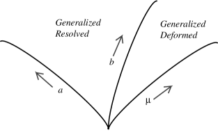
Figure 2.3: Representation of the moduli space of generalized resolutions of the conifold singularity. The two regions depicted correspond to the two solutions of our constraint. The generalized deformed conifold metric is singular. A point on each of the three lines represents, from left to right, the resolved, regularized and deformed conifold. They meet at a single point, the singular conifold.

As a byproduct of the supersymmetry analysis, the Killing spinors for these geometries have been obtained. In particular, the obtainment of the Killing spinors on the deformed conifold is remarkable. It is based on a rotated radial projection (2.2.29). We will see in the following chapters that this technical trick is really useful, since such kind of rotated projection appears in lots of setups.

Moreover, it has been shown that lower-dimensional gauged supergravities are an appropriate framework to resolve singularities in the study of geometries corresponding to D-branes wrapping supersymmetric cycles, which are dual to supersymmetric gauge theories. A conventional twisting (2.2.6) with $g=0$ and constant $\lambda$ leads to the singular conifold metric. But as we have seen, by switching on the appropriate degrees of freedom of the gauged sugra, the twisting can be generalized and the singularity smoothened. However, asymptotically (for large $r$), the solution, and therefore, the twisting, remains unaltered.

Finally, it is worth to point out that the mechanism presented in this chapter for desingularizing the conifold is also useful to study other singularity resolutions. Some examples will be presented in the following.

Chapter 3 $G_{2}$ holonomy metrics from gauged supergravity

3.1 Introduction

$G_{2}$ holonomy manifolds and their physical significance

On a Riemannian manifold, one can move tangent vectors along a path by parallel transport. The holonomy group is defined as the set of linear transformations arising from parallel transport along closed loops. As parallel transport preserves the length of vectors, the holonomy group of an orientable $n$-manifold must be contained in $SO(n)$. If it is indeed a proper subgroup, then we say that the manifold has special holonomy. Special holonomy manifolds are important in physics because they preserve some fraction of the supersymmetry (we have already seen an example in the previous chapter, the conifold, which has $SU(3)$ holonomy and, hence, it is 1/4-supersymmetric). In this chapter we will consider manifolds with $G_{2}$ holonomy.

The group $G_{2}$ is a subgroup of $SO(7)$, so we will deal with seven dimensional manifolds. It leaves invariant the multiplication table of the imaginary octonions. Therefore, its action preserves the form:

$$\Phi_{(3)}=dx_{123}+dx_{145}+dx_{167}+dx_{246}-dx_{257}-dx_{347}-dx_{356}\,\,.$$ (3.1.1)

Then in order to have $G_{2}$ holonomy, there must exist such a three-form that does not change under parallel transport throughout the manifold. Referring the three-form to some vielbein basis, we need its covariant derivative to vanish: $D_{\mu}\Phi_{\nu\rho\sigma}=0$. It is known that this is equivalent to having:

$$d\Phi\,=\,d{}^{*}\Phi\,=\,0\,\,.$$ (3.1.2)

$\Phi$ is a calibrating three-form which calibrates a minimal three-cycle inside the seven dimensional $G_{2}$ holonomy geometry. This cycle is called associative (the four-cycle calibrated by ${}^{*}\Phi$ is called coassociative).

Let us now turn to the relation of $G_{2}$ holonomy with supersymmetry. The spinor representation of $SO(7)$ can be decomposed, in terms of representations of $G_{2}$, as:

$${\bf 8}\,\rightarrow\,{\bf 7}\,+\,{\bf 1}\,\,,$$ (3.1.3)

i.e. it splits into a fundamental and a singlet of $G_{2}$. Only the singlet gives a covariantly constant spinor $D_{\mu}\epsilon=0$. The rest of the spinors get changed under transport over the manifold. Hence, $G_{2}$ holonomy manifolds are 1/8-supersymmetric. Going now to eleven dimensional supergravity, one can conclude that, being supersymmetric, it solves the equations of motion, and, therefore, $G_{2}$ holonomy manifolds are Ricci-flat (we set the 3-form of D=11 sugra to zero). It is also worth to point out that the three-form $\Phi$ can be computed as a bilinear in the covariantly constant spinor. This property will be explicitly used in sections 3.2.2 and 3.3.2 below. It gives a relation between the projections on the Killing spinors and the calibrating form.

For a better introduction to all the topics presented above, see [45].

By studying M-theory on $G_{2}$ holonomy manifolds, one finds a dual description of ${\cal N}=1$ four dimensional supersymmetric Yang-Mills (SYM). If the manifold is large enough and smooth, the low energy description is given in terms of a purely gravitational configuration of eleven dimensional supergravity. The gravity/gauge theory correspondence then allows for a geometrical approach to the study of important aspects of the strong coupling regime of SYM theory such as the existence of a mass gap, chiral symmetry breaking, confinement, gluino condensation, domain walls and chiral fermions [40, 46, 47, 48]. These facts have led, in the last years, to a concrete and important physical motivation to study compact and non–compact seven-manifolds of $G_{2}$ holonomy.

Up to year 2001, there were only three known examples of complete metrics with $G_{2}$ holonomy on Riemannian manifolds [49, 50]. They correspond to ${\rm I\kern-1.6pt{\rm R}}^{3}$ bundles over $S^{4}$ or ${{\mathchoice{\rm C\mkern-8.0mu\vrule height=6.24301pt,depth=-0.21529pt,width=0.50003pt\mkern 9.0mu\kern-0.50003pt}{\rm C\mkern-8.0mu\vrule height=6.24301pt,depth=-0.21529pt,width=0.50003pt\mkern 9.0mu\kern-0.50003pt}{\rm C\mkern-8.0mu\vrule height=4.30554pt,depth=-0.3014pt,width=0.35004pt\mkern 9.0mu\kern-0.35004pt}{\rm C\mkern-8.0mu\vrule height=2.79857pt,depth=-0.43057pt,width=0.24994pt\mkern 8.0mu\kern-0.24994pt}}{\rm I\kern-1.79993ptP}}^{2}$, and to an ${\rm I\kern-1.6pt{\rm R}}^{4}$ bundle over $S^{3}$. These manifolds develop isolated conical singularities corresponding, respectively, to cones on ${{\mathchoice{\rm C\mkern-8.0mu\vrule height=6.24301pt,depth=-0.21529pt,width=0.50003pt\mkern 9.0mu\kern-0.50003pt}{\rm C\mkern-8.0mu\vrule height=6.24301pt,depth=-0.21529pt,width=0.50003pt\mkern 9.0mu\kern-0.50003pt}{\rm C\mkern-8.0mu\vrule height=4.30554pt,depth=-0.3014pt,width=0.35004pt\mkern 9.0mu\kern-0.35004pt}{\rm C\mkern-8.0mu\vrule height=2.79857pt,depth=-0.43057pt,width=0.24994pt\mkern 8.0mu\kern-0.24994pt}}{\rm I\kern-1.79993ptP}}^{3}$, $SU(3)/U(1)\times U(1)$, or $S^{3}\times S^{3}$.

Constructing additional complete metrics can be an important issue in improving our understanding of the strongly coupled infrared dynamics of ${\cal N}=1$ supersymmetric gauge theories. For example, a new $G_{2}$ holonomy manifold with an asymptotically stabilized $S^{1}$ was recently found [51]. This solution is asymptotically locally conical (ALC) –near infinity it approaches a circle bundle with fibres of constant length over a six–dimensional cone–, as opposed to the asymptotically conical (AC) solutions found in [49, 50].

The rôle of gauged supergravity

Salam-Sezgin eight dimensional gauged supergravity (see section 1.4.4) is an appropriate tool for obtaining a large family of $G_{2}$ holonomy metrics. Once again, the reason is that the natural framework to study D6-branes is an eight dimensional theory, where the D6’s are domain walls.

A ten dimensional configuration where D6-branes wrap a special Lagrangian three-cycle inside a Calabi-Yau three-fold uplifts to $G_{2}$ holonomy manifolds in eleven dimensions. This is deduced from supersymmetry and holonomy matching conditions [34]. We will consider an eight dimensional ansatz corresponding to D6-branes wrapping a cycle which is topologically $S^{3}$. When uplifting to M-theory, there is another $S^{3}$, so the metrics obtained will have $S^{3}\times S^{3}$ principal orbits. Furthermore, they will have cohomogeneity one (corresponding to the radial direction). At small $r$, one of the spheres shrinks yielding the topology of an ${\rm I\kern-1.6pt{\rm R}}^{4}$ bundle over $S^{3}$ (so the solutions with the other topologies cannot be found by this procedure).

All known metrics of this kind will be found below from gauged supergravity, as solutions of a single system of equations [9]. Actually, we will recover Hitchin’s general system [52] from a different approach. The calibrating forms and Killing spinors are also computed.

Notably, the set of solutions comprises the ALC ones, what proves what a powerful tool gauged sugra can be. That such metrics are obtained may seem surprising, as the archetypical ALC metric is Taub-NUT space, which corresponds to the eleven dimensional description of the full supergravity solution describing D6-branes in flat space. It was argued in [53] that D=8 gauged supergravity only accounts for the near-horizon physics of D6-branes, thus leading to the Eguchi-Hanson solution, in which there is no stabilized circle.

Indeed, let us take the eight dimensional ansatz [54]:

$$ds_{8}^{2}\,=\,e^{2\phi\over 3}\,dx_{1,6}^{2}\,+\,dr^{2}\,\,,$$ (3.1.4)

and excite one of the scalars in the coset, as in eq. (2.2.2). There is no gauge field in this case. By imposing the projection:

$$\Gamma_{r}\hat{\Gamma}_{123}\,\epsilon\,=\,-\,\epsilon\,\,,$$ (3.1.5)

the BPS eqs. coming from the vanishing of the fermion field susy variations (1.4.29) read:

$$\phi^{\prime} = {1\over 8}\,e^{-\phi}\,(e^{-4\lambda}\,+\,2\,e^{2\lambda})\,\,,$$

$$\lambda^{\prime} = {1\over 6}\,e^{-\phi}\,(e^{-4\lambda}\,-\,e^{2\lambda})\,\,,$$ (3.1.6)

whereas if $\eta$ is a constant spinor satisfying $\Gamma_{r}\hat{\Gamma}_{123}\eta=-\eta$, one has $\epsilon=e^{{\phi\over 6}}\eta$. Changing the radial variable as $dr=e^{\phi-2\lambda}dt$, the BPS system can be easily solved:

$$\lambda={1\over 6}\left[\log(e^{t}+a^{4})-t\,\right]\,\,,\qquad\qquad\phi={3\over 4}\left[\lambda+{1\over 2}t-\log(16)\,\right]\,\,,$$ (3.1.7)

where we have appropriately defined the integration constants. Let us make another redefinition of the radial variable: $e^{t}=\rho^{4}-a^{4}$. Then, the eleven dimensional solution (1.4.24) reads $ds_{11}^{2}=dx_{1,6}^{2}+ds_{EH}^{2}$ and we find the (1/2-supersymmetric) Eguchi-Hanson metric (see, for example, [55]):

$$ds_{EH}^{2}\,=\,{1\over 1-{a^{4}\over\rho^{4}}}\,d\rho^{2}\,+\,{\rho^{2}\over 4}\,\left[(\tilde{w}^{1})^{2}+(\tilde{w}^{2})^{2}+\left(1-{a^{4}\over\rho^{4}}\right)(\tilde{w}^{3})^{2}\,\right]\,\,.$$ (3.1.8)

On the other hand, the ALC Ricci-flat Taub-NUT metric reads [55]:

$$ds_{Taub-NUT}^{2}\,=\,{1\over 4}{r+m\over r-m}dr^{2}+{1\over 4}(r^{2}-m^{2})\left[(\tilde{w}^{1})^{2}+(\tilde{w}^{2})^{2}\right]+m^{2}\,{r-m\over r+m}\,(\tilde{w}^{3})^{2}\,\,.$$ (3.1.9)

There is also a multi-center version of this solution corresponding to parallel, but not coincident, D6-branes.

3.2 D6-brane wrapped on $S^{3}$

For the sake of clarity, let us start by analyzing the case that corresponds to a D6-brane wrapping a three–cycle in such a way that the corresponding eight dimensional metric $ds^{2}_{8}$ contains a round three-sphere. The general, much more involved, ansatz (allowing anisotropy of the $S^{3}$) will be addressed in section 3.3. Accordingly, we consider now the following metric:

$$ds^{2}_{8}\,=\,e^{{2\phi\over 3}}\,dx_{1,3}^{2}\,+\,e^{2h}\,d\Omega_{3}^{2}\,+\,dr^{2}\,\,,$$ (3.2.1)

where $dx_{1,3}^{2}=-(dx^{0})^{2}+(dx^{1})^{2}+(dx^{2})^{2}+(dx^{3})^{2}$, $\phi$ and $h$ are functions of the radial coordinate $r$ and $d\Omega_{3}^{2}$ is the metric of the unit $S^{3}$. The factor on the unwrapped directions has been chosen as in (2.2.10) to have Minkowski space in those directions after uplifting. It is convenient to parametrize the three-sphere by means of a new set of left invariant one-forms $w^{i}$, $i=1,2,3$, of the $SU(2)$ group manifold like the ones defined in (1.4.27). (The symbol $\tilde{w}^{i}$ will continue to denote the forms of the $S^{3}$ involved in the reduction from eleven to eight dimensions.) So we have:

$$d\Omega_{3}^{2}\,=\,{1\over 4}\,\sum_{i=1}^{3}\,(\,w^{i}\,)^{2}\,\,.$$ (3.2.2)

In the configurations studied in the present section, apart from the metric, we will only need to excite the dilatonic scalar $\phi$ and the $SU(2)$ gauge potential $A_{\mu}^{i}$. As the scalars in the coset are trivial ($\lambda=0$ in the notation of (2.2.2)), we get the following simple values for the tensors appearing in the Salam-Sezgin formalism:

$$T_{ij}\,=\,\delta_{ij}\,\,,\,\,\,\,\,\,\,\,\,\,P_{ij}\,=\,0\,\,,\,\,\,\,\,\,\,\,\,\,Q_{ij}=\pmatrix{0&&-A^{3}&&A^{2}\cr A^{3}&&0&&-A^{1}\cr-A^{2}&&A^{1}&&0}\,\,.$$ (3.2.3)

We will assume that the non-abelian gauge potential $A_{\mu}^{i}$ has only non-vanishing components along the directions of the $S^{3}$. Actually, we will adopt an ansatz in which this field, written as a one-form, is given by:

$$A^{i}\,=\,\Big{(}\,g\,-\,{1\over 2}\,\Big{)}\,w^{i}\,\,,$$ (3.2.4)

with $g$ being a function of the radial coordinate $r$. The field strength corresponding to the potential (3.2.4) is (the prime denotes derivative with respect to $r$):

$$F^{i}\,=\,g^{\prime}\,dr\,\wedge\,w^{i}\,+\,{1\over 8}\,(\,4g^{2}-1\,)\,\epsilon^{ijk}\,w^{j}\,\wedge\,w^{k}\,\,.$$ (3.2.5)

The eleven dimensional metric reads (1.4.24):

$$ds_{11}^{2}\,=\,dx_{1,3}^{2}\,+\,e^{-\frac{2\phi}{3}}\,dr^{2}\,+\,{1\over 4}\,e^{2h-\frac{2\phi}{3}}\,w_{i}^{2}\,+\,4\,e^{\frac{4\phi}{3}}\,\left(\tilde{w}^{i}+(g-{1\over 2})\,w^{i}\right)^{2}$$ (3.2.6)

This ansatz extends the one used in [43] to get a metric of $G_{2}$ holonomy by the inclusion of the function $g$. We will see that the key point for having $g\neq 0$ is that a rotated projection similar to (2.2.29) is needed.

3.2.1 Supersymmetry analysis

In this section we will find a system of first-order equations by analyzing the supersymmetry transformations of the fermionic fields, along the lines of section 1.3.1. As we will verify soon, this approach will give us the hints we need to extend our analysis to metrics more general than the one written in eq. (3.2.1).

In what follows, the Dirac matrices along the sphere $S^{3}$ shall be denoted by $\{\Gamma_{1},\Gamma_{2},\Gamma_{3}\}$, while, as before, $\{\hat{\Gamma}_{1},\hat{\Gamma}_{2},\hat{\Gamma}_{3}\}$ will be the matrices along the $SU(2)$ group manifold.

The first-order BPS equations we are trying to find are obtained by requiring that $\delta\chi_{i}=\delta\psi_{\lambda}=0$ (1.4.29) for some Killing spinor $\epsilon$, which must satisfy some projection conditions. First of all, we need to impose that:

$$\Gamma_{12}\,\epsilon\,=\,-\hat{\Gamma}_{12}\,\epsilon\,\,,\,\,\,\,\,\,\,\,\,\,\,\,\,\,\,\Gamma_{23}\,\epsilon\,=\,-\hat{\Gamma}_{23}\,\epsilon\,\,,\,\,\,\,\,\,\,\,\,\,\,\,\,\,\,\Gamma_{13}\,\epsilon\,=\,-\hat{\Gamma}_{13}\,\epsilon\,\,.$$ (3.2.7)

Notice that in eq. (3.2.7) the projections along the sphere $S^{3}$ and the $SU(2)$ group manifold are related. Actually, only two of these equations are independent and, for example, the last one can be obtained from the first two. Moreover, it follows from (3.2.7) that:

$$\Gamma_{1}\hat{\Gamma}_{1}\epsilon\,=\,\Gamma_{2}\hat{\Gamma}_{2}\epsilon\,=\,\Gamma_{3}\hat{\Gamma}_{3}\epsilon\,\,.$$ (3.2.8)

These projections are imposed by the ambient Calabi–Yau three–fold in which the three–cycle lives, from the conditions $J_{ab}~{}\epsilon=\Gamma_{ab}~{}\epsilon$, where $J$ is the Kähler form. By using eqs. (3.2.7) and (3.2.8) to evaluate the right-hand side of (1.4.29), together with the ansatz for the metric, dilaton and gauge field, one gets some equations which give the radial derivative of $\phi$, $h$ and $\epsilon$. Actually, one arrives at the following equation for the radial derivative of the dilaton:

$$\phi^{\prime}\epsilon\,=\,{3\over 8}\,\Big{[}\,4\,(\,1-4g^{2}\,)\,e^{\phi-2h}\,-\,e^{-\phi}\,\Big{]}\,\Gamma_{r}\,\hat{\Gamma}_{123}\,\epsilon\,+\,3\,e^{\phi-h}\,g^{\prime}\,\Gamma_{1}\,\hat{\Gamma}_{1}\,\epsilon\,\,,$$ (3.2.9)

while the derivative of the function $h$ is:

$$h^{\prime}\epsilon = 2ge^{-h}\,\Gamma_{1}\,\hat{\Gamma}_{1}\,\Gamma_{r}\,\hat{\Gamma}_{123}\,\epsilon\,-\,{1\over 8}\,\Big{[}\,12\,(\,1-4g^{2}\,)\,e^{\phi-2h}\,+\,e^{-\phi}\,\Big{]}\,\Gamma_{r}\,\hat{\Gamma}_{123}\,\epsilon\,-\,$$ (3.2.10)

$$-\,e^{\phi-h}\,g^{\prime}\,\Gamma_{1}\,\hat{\Gamma}_{1}\,\epsilon\,\,.$$

Moreover, the radial dependence of the spinor $\epsilon$ is determined by:

$$\partial_{r}\,\epsilon\,-\,{1\over 16}\,\Big{[}\,4(\,1-4g^{2}\,)\,e^{\phi-2h}\,\,-\,e^{-\phi}\,\Big{]}\,\Gamma_{r}\,\hat{\Gamma}_{123}\,\epsilon\,+\,{5\over 2}\,e^{\phi-h}\,g^{\prime}\,\Gamma_{1}\,\hat{\Gamma}_{1}\,\epsilon\,=\,0\,\,.$$ (3.2.11)

In order to proceed further, we need to impose some additional condition to the spinor $\epsilon$. It is clear from the right-hand side of eqs. (3.2.9)-(3.2.11) that we must specify the action on $\epsilon$ of the radial projector $\Gamma_{r}\,\hat{\Gamma}_{123}$. The choice made in ref. [43] was to take $g=0$ and impose the condition $\Gamma_{r}\,\hat{\Gamma}_{123}\,\epsilon\,=\,-\epsilon$. It is immediate to verify that in this case the eqs. (3.2.9)–(3.2.11) reduce to those obtained in ref. [43]. Here we will not take any a priori particular value of $\Gamma_{r}\,\hat{\Gamma}_{123}\,\epsilon$. Instead we will try to determine it in general from eqs. (3.2.9)–(3.2.11). Notice that in our approach $g$ will not be constant and, therefore, we will have to find a differential equation which determines it. It is clear from eq. (3.2.9) that our spinor $\epsilon$ must satisfy a relation of the sort of (2.2.17):

$$\Gamma_{r}\,\hat{\Gamma}_{123}\,\epsilon\,=\,-(\beta\,+\,\tilde{\beta}\,\Gamma_{1}\,\hat{\Gamma}_{1}\,)\,\epsilon\,\,,$$ (3.2.12)

where $\beta$ and $\tilde{\beta}$ are again functions of the radial coordinate $r$, which in this case can be easily extracted from eq. (3.2.9), namely:

$$\beta = -{8\over 3}\,\,{\phi^{\prime}\over 4(1-4g^{2})\,e^{\phi-2h}\,-\,e^{-\phi}}\,\,,$$

$$\tilde{\beta} = 8\,\,{e^{\phi-h}\,g^{\prime}\over 4(1-4g^{2})\,e^{\phi-2h}\,-\,e^{-\phi}}\,\,.$$ (3.2.13)

As in the previous chapter, the consistency condition:

$$\beta^{2}\,+\,\tilde{\beta}^{2}\,=\,1\,\,,$$ (3.2.14)

holds. This can be proved by noticing that $(\Gamma_{r}\,\hat{\Gamma}_{123})^{2}\epsilon\,=\,\epsilon$ and that $\{\Gamma_{r}\,\hat{\Gamma}_{123},\Gamma_{1}\,\hat{\Gamma}_{1}\}=0$. By using in eq. (3.2.14) the explicit values of $\beta$ and $\tilde{\beta}$ given in eq. (3.2.13), one gets:

$${(\phi^{\prime})^{2}\over 9}\,+\,e^{2\phi-2h}\,(g^{\prime})^{2}\,=\,{1\over 64}\,\Big{[}\,4(1-4g^{2})\,e^{\phi-2h}\,-\,e^{-\phi}\,\Big{]}^{2}\,\,,$$ (3.2.15)

which relates the radial derivatives of $\phi$ and $g$. Let us now consider the equation for $h^{\prime}$ written in eq. (3.2.10). By using the value of $\Gamma_{r}\,\hat{\Gamma}_{123}\,\epsilon$ given in eq. (3.2.12), and separating the terms with and without $\Gamma_{1}\,\hat{\Gamma}_{1}\,\epsilon$, we get two equations:

$$h^{\prime}\,=\,2ge^{-h}\,\tilde{\beta}\,+\,{1\over 8}\,\Big{[}\,\,12(1-4g^{2})\,e^{\phi-2h}\,+\,e^{-\phi}\,\Big{]}\,\beta\,\,,$$

$$2g\,e^{-h}\,\beta\,-\,{1\over 8}\,\Big{[}\,\,12(1-4g^{2})\,e^{\phi-2h}\,+\,e^{-\phi}\,\Big{]}\,\tilde{\beta}\,+\,e^{\phi-h}\,g^{\prime}\,=\,0\,\,.$$ (3.2.16)

Moreover, by using in the latter the values of $\beta$ and $\tilde{\beta}$ given in eq. (3.2.13), we get the following relation between $g^{\prime}$ and $\phi^{\prime}$:

$$g^{\prime}\,=\,-{8g\over 3}\,{e^{2h}\,\phi^{\prime}\over 4(1-4g^{2})\,e^{2\phi}\,+\,e^{2h}}\,\,.$$ (3.2.17)

Plugging back this equation in the consistency condition (3.2.15), we can determine $\phi^{\prime}$, $g^{\prime}$, $\beta$ and $\tilde{\beta}$ in terms of $\phi$, $g$ and $h$. Moreover, by substituting these results on the first equation in (3.2.16), we get a first-order equation for $h$. In order to write these equations, let us define the function:

$$K\equiv\sqrt{\Big{(}\,4\,(1-2g)^{2}\,e^{2\phi}+\,e^{2h}\,\Big{)}\,\Big{(}\,4\,(1+2g)^{2}\,e^{2\phi}+\,e^{2h}\,\Big{)}}\,\,.$$ (3.2.18)

Then, the BPS equations are:

$$\phi^{\prime} = \,{3\over 8}\,\,{e^{-2h-\phi}\over K}\,\,\Big{[}\,e^{4h}\,-\,16\,(1-4g^{2})^{2}\,e^{4\phi}\,\Big{]}\,\,,$$

$$h^{\prime} = {e^{-2h-\phi}\over 8K}\,\,\Big{[}\,e^{4h}\,+\,16\,(1+4g^{2})\,e^{2h+2\phi}\,+\,48\,(1-4g^{2})^{2}\,e^{4\phi}\,\Big{]}\,\,,$$

$$g^{\prime} = {ge^{-\phi}\over K}\,\,\Big{[}\,4\,(1-4g^{2})\,e^{2\phi}\,-\,e^{2h}\,\Big{]}\,\,.$$ (3.2.19)

Notice that $g^{\prime}=g=0$ certainly solves the last of these equations and, in this case, the square root disappears from $K$ and the first two equations in (3.2.19) reduce to the ones written in ref. [43]. Moreover, the system (3.2.19) is identical to that found in ref. [56] by means of the superpotential method (see section 3.2.4). The solutions of (3.2.19) have been obtained in ref. [56], and they depend on two parameters (see section 3.2.3).

The radial projection can be interpreted as in section 2.2, where a similar expression was reached studying the conifold. We can parametrize $\beta=\cos\alpha$ and $\tilde{\beta}=\sin\alpha$, as in (2.2.21), and by substituting the value of $\phi^{\prime}$ and $g^{\prime}$ given by the first-order equations (3.2.19) into the definition of $\beta$ and $\tilde{\beta}$ (eq. (3.2.13)), one arrives at:

$$\tan\alpha\,=\,8g\,{e^{\phi+h}\over 4(1-4g^{2})\,e^{2\phi}\,+\,e^{2h}}\,\,.$$ (3.2.20)

Then, by using the representation (2.2.21), it is immediate to rewrite eq. (3.2.12) as:

$$\Gamma_{r}\,\hat{\Gamma}_{123}\,\epsilon\,=\,-e^{\alpha\Gamma_{1}\hat{\Gamma}_{1}}\,\,\epsilon\,\,.$$ (3.2.21)

Since $\{\Gamma_{r}\,\hat{\Gamma}_{123},\Gamma_{1}\,\hat{\Gamma}_{1}\}=0$, eq. (3.2.21) can be solved as:

$$\epsilon\,=\,e^{-{1\over 2}\alpha\Gamma_{1}\hat{\Gamma}_{1}}\,\,\epsilon_{0}\,\,,$$ (3.2.22)

where $\epsilon_{0}$ is a spinor satisfying the standard radial projection condition with $\alpha=0$, i.e.:

$$\Gamma_{r}\,\hat{\Gamma}_{123}\,\epsilon_{0}\,=\,-\epsilon_{0}\,\,.$$ (3.2.23)

To determine completely $\epsilon_{0}$ we must use eq. (3.2.11), which dictates the radial dependence of the Killing spinor. Actually, by using the first-order equations (3.2.19) one can compute $\partial_{r}\,\alpha$ from eq. (3.2.20). The result is remarkably simple, namely:

$$\partial_{r}\,\alpha\,=\,6\,e^{\phi-h}\,g^{\prime}\,\,.$$ (3.2.24)

By using eq. (3.2.22) in eq. (3.2.11), one consistently obtains (3.2.24) again. Furthermore, the typical radial dependence of $\epsilon_{0}$ in terms of the dilaton (2.2.31) is found. Thus, after collecting all results, it follows that $\epsilon$ can be written as:

$$\epsilon\,=\,e^{{\phi\over 6}}\,e^{-{1\over 2}\alpha\Gamma_{1}\hat{\Gamma}_{1}}\,\eta\,\,.$$ (3.2.25)

The projections conditions satisfied by $\eta$ are simply:

$$\Gamma_{12}\,\hat{\Gamma}_{12}\,\eta\,=\,\eta\,\,,\,\,\,\,\,\,\,\,\,\,\,\,\,\,\,\,\,\,\,\,\,\,\,\,\Gamma_{23}\,\hat{\Gamma}_{23}\,\eta\,=\,\eta\,\,,\,\,\,\,\,\,\,\,\,\,\,\,\,\,\,\,\,\,\,\,\,\,\,\,\Gamma_{r}\,\hat{\Gamma}_{123}\,\eta\,=\,-\eta\,\,.$$ (3.2.26)

In order to find out the meaning of the phase $\alpha$, let us use (1.4.32) to write the radial projection (3.2.21) as:

$$\Gamma_{x^{0}\cdots x^{3}}\,\big{(}\,\cos\alpha\Gamma_{123}\,-\,\sin\alpha\hat{\Gamma}_{123}\,\big{)}\,\epsilon\,=\,\epsilon\,\,,$$ (3.2.27)

which is the projection corresponding to a D6–brane wrapped on a three–cycle, which is non-trivially embedded in the two three–spheres, with $\alpha$ measuring the contribution of each sphere. This equation must be understood as seen from the uplifted perspective. The case $\alpha=0$ corresponds to the D6–brane wrapping a three–sphere that is fully contained in the eight–dimensional space-time where supergravity lives, and has been studied earlier [43]. Notice that $\alpha=\pi/2$ is not a solution of the system. This is an important consistency check as this would mean that the D6–brane is not wrapping a three–cycle contained in the eight–dimensional space-time and the twisting would make no sense. However, solutions that asymptotically approach $\alpha=\pi/2$ are possible. In the next subsection we will describe a quantity for which the rotation by the angle $\alpha$ plays an important rôle.

3.2.2 The calibrating three-form

Given a solution of the BPS equations (3.2.19), one can get an eleven dimensional metric $ds^{2}_{11}$ by means of the uplifting formula (1.4.24). The corresponding eleven dimensional manifold is a direct product of four dimensional Minkowski space and a seven dimensional manifold, i.e.:

$$ds^{2}_{11}\,=\,dx^{2}_{1,3}\,+\,ds^{2}_{7}\,=\,dx^{2}_{1,3}\,+\,\sum_{A=1}^{7}\,\big{(}\,e^{A}\,)^{2}\,\,,$$ (3.2.28)

where we have written $ds^{2}_{7}$ in terms of a basis of one-forms $e^{A}$ ($A=1,\cdots,7)$. It follows from (1.4.24) that this basis can be taken as:

$$e^{i} = {1\over 2}\,e^{h-{\phi\over 3}}\,\,w^{i}\,,\,\,\,\,\,\,\,\,\,\,(i=1,2,3)\,\,,$$

$$e^{3+i} = 2\,e^{{2\phi\over 3}}\,\big{(}\,\tilde{w}^{i}\,+\,(\,g-{1\over 2}\,)\,w^{i}\,\,\big{)}\,,\,\,\,\,\,\,\,\,\,\,(i=1,2,3)\,\,,$$

$$e^{7} = e^{-{\phi\over 3}}\,dr\,\,.$$ (3.2.29)

It is a well-known fact that a manifold of $G_{2}$ holonomy is endowed with a calibrating three-form $\Phi$, which must be closed and co-closed (as stated in eq. (3.1.2)) with respect to the seven dimensional metric $ds^{2}_{7}$. We shall denote by $\phi_{ABC}$ the components of $\Phi$ in the basis $(\ref{tcinco})$, namely:

$$\Phi\,=\,{1\over 3!}\,\phi_{ABC}\,e^{A}\wedge e^{B}\wedge e^{C}\,\,.$$ (3.2.30)

The relation between $\Phi$ and the Killing spinors of the metric is also well-known. Indeed, let $\tilde{\epsilon}$ be the Killing spinor uplifted to eleven dimensions, which in terms of $\epsilon$ is simply $\tilde{\epsilon}=e^{-{\phi\over 6}}\,\epsilon$. Then, one has:

$$\phi_{ABC}\,=\,i\,\tilde{\epsilon}^{\dagger}\,\Gamma_{ABC}\,\tilde{\epsilon}\,\,.$$ (3.2.31)

By using the relation between $\epsilon$ and the constant spinor $\eta$, one can rewrite eq. (3.2.31) as:

$$\phi_{ABC}\,=\,i\,\eta^{\dagger}\,e^{{1\over 2}\alpha\Gamma_{1}\hat{\Gamma}_{1}}\Gamma_{ABC}\,e^{-{1\over 2}\alpha\Gamma_{1}\hat{\Gamma}_{1}}\eta\,\,.$$ (3.2.32)

Let us now denote by $\phi_{ABC}^{(0)}$ the above matrix element when $\alpha=0$, i.e.:

$$\phi_{ABC}^{(0)}\,=\,i\,\eta^{\dagger}\,\Gamma_{ABC}\,\eta\,\,.$$ (3.2.33)

It is not difficult to obtain the non-zero matrix elements of (3.2.33). Recall that $\eta$ is characterized as an eigenvector of the set of projection operators written in eq. (3.2.26). Thus, if ${\cal O}$ is an operator which anticommutes with any of these projectors, ${\cal O}\eta$ and $\eta$ are eigenvectors of the projectors with different eigenvalues and, therefore, they are orthogonal (i.e. $\eta^{\dagger}{\cal O}\eta=0$). Moreover, by using the projection conditions (3.2.26), one can relate the non-vanishing matrix elements to $\eta^{\dagger}\,\Gamma_{123}\,\eta$. If we normalize $\eta$ such that $i\,\eta^{\dagger}\,\Gamma_{123}\,\eta\,=\,1$ and if $\hat{i}\,=\,i+3$ for $i=1,2,3$, one can easily prove that the non-zero $\phi_{ijk}^{(0)}$’s are:

$$\phi_{ijk}^{(0)}\,=\,\epsilon_{ijk}\,\,,\,\,\,\,\,\,\,\,\,\,\,\,\,\,\,\,\,\,\phi_{i\hat{j}\hat{k}}^{(0)}\,=\,-\epsilon_{ijk}\,\,,\,\,\,\,\,\,\,\,\,\,\,\,\,\,\,\,\,\,\phi_{7i\hat{j}}^{(0)}\,=\,\delta_{ij}\,\,,$$ (3.2.34)

as in [57]. This form is like the one written in (3.1.1) after a relabelling of the indices. By expanding the exponential in (3.2.32) and using (3.2.34), it is straightforward to find the different components of $\Phi$ for arbitrary $\alpha$. Actually, one can write the result as:

$$\Phi = e^{7}\,\wedge\,\big{(}\,e^{1}\,\wedge\,e^{4}\,+\,e^{2}\,\wedge\,e^{5}\,+\,e^{3}\,\wedge\,e^{6}\,\big{)}\,+\,$$ (3.2.35)

$$+\,\big{(}\,e^{1}\cos\alpha+e^{4}\sin\alpha\,\big{)}\,\wedge\,\big{(}\,e^{2}\wedge e^{3}-e^{5}\wedge e^{6}\,\big{)}\,+$$

$$+\,\big{(}\,-e^{1}\sin\alpha+e^{4}\cos\alpha\,\big{)}\,\wedge\,\big{(}\,e^{3}\wedge e^{5}-e^{2}\wedge e^{6}\,\big{)}\,\,,$$

which shows that the effect on $\Phi$ of introducing the phase $\alpha$ is just a (radial dependent) rotation in the $(e^{1},e^{4})$ plane (alternatively, the same expression can be written as a rotation in the $(e^{2},e^{5})$ or $(e^{3},e^{6})$ plane). As mentioned above, $\Phi$ should be closed and co-closed:

$$d\Phi=0\,\,,\,\,\,\,\,\,\,\,\,\,\,\,\,\,\,\,\,\,d*_{7}\Phi=0\,\,,$$ (3.2.36)

where $*_{7}$ denotes the Hodge dual in the seven dimensional metric. There is an immediate consequence of this fact which we shall now exploit. Let us denote by $p$ and $q$ the components of $\Phi$ along the volume forms of the two three spheres, i.e.:

$$\Phi\,=\,p\,\,w^{1}\wedge w^{2}\wedge w^{3}\,+\,q\,\,\tilde{w}^{1}\wedge\tilde{w}^{2}\wedge\tilde{w}^{3}\,+\,\cdots\,\,.$$ (3.2.37)

From the condition $d\Phi=0$, it follows immediately that $p$ and $q$ must be constant. By plugging the explicit expression of the forms $e^{A}$, given in eq. (3.2.29), on the right-hand side of eq. (3.2.35), one easily gets $p$ and $q$ in terms of $\phi$, $h$ and $g$. Thus, the two constant of motion are:

$$p = {1\over 8}\,\Big{[}\,e^{3h-\phi}\,-\,12\,e^{h+\phi}\,\,(\,1-2g\,)^{2}\,\Big{]}\,\cos\alpha\,-\,{1\over 4}\,(1-2g)\,\Big{[}\,3e^{2h}\,-\,4\,e^{2\phi}\,(\,1-2g\,)^{2}\,\Big{]}\,\sin\alpha\,\,,$$

$$q = -8e^{2\phi}\,\sin\alpha\,\,.$$ (3.2.38)

Notice that $\alpha=0$ implies $q=0$ which is precisely the case studied in [43]. By explicit calculation one can check that $p$ and $q$ are constants as a consequence of the BPS equations. Actually, by using (3.2.19) one can show that, indeed, $\Phi$ is closed and co-closed as it should.

3.2.3 Solving the equations

The Bryant-Salamon metric

As argued above, one can take consistently $g=0$, going back to the analysis of [43]. In this case, the system of equations (3.2.19) gets drastically simplified:

$$\phi^{\prime}\, = \,\frac{3}{8}\,e^{-\phi}\,-\,\frac{3}{2}\,e^{\phi-2h}\,\,,$$

$$h^{\prime}\, = \,\frac{1}{8}\,e^{-\phi}\,+\,\frac{3}{2}\,e^{\phi-2h}\,\,.$$ (3.2.39)

Let us define a new function $x$ and a new radial variable $t$:

$$x\equiv 12\,e^{2\phi-2h}\,\,,\,\,\,\,\,\,\,\,\,\,\,\,\,\,\,\frac{dr}{dt}\,=\,e^{\phi}\,\,.$$ (3.2.40)

Then, eq. (2.3.4) is obtained again, and therefore:

$$x\,=\,{1\over 1\,+\,b\,e^{-\frac{t}{2}}}\,\,\,,$$ (3.2.41)

that immediately leads to:

$$e^{2h}\,=\,e^{\frac{t}{4}}\,(b\,+\,e^{\frac{t}{2}})^{1\over 2}\,\,,\,\,\,\,\,\,\,\,\,\,\,\,\,\,\,e^{2\phi}\,=\,\frac{1}{12}\,e^{\frac{3t}{4}}\,(b\,+\,e^{\frac{t}{2}})^{-{1\over 2}}\,\,.$$ (3.2.42)

The solution is better expressed by redefining the integration constant and the radial coordinate:

$$b\,\equiv\frac{a^{3}}{18}\,\,,\,\,\,\,\,\,\,\,\,\,\,\,\,\,\,e^{\frac{t}{2}}\equiv{1\over 18}\,(\rho^{3}-a^{3})\,\,,$$ (3.2.43)

in terms of which (3.2.42) reads:

$$e^{2h}\,=\,\frac{\rho^{3}}{18}\,\,\left(1-\frac{a^{3}}{\rho^{3}}\right)^{1\over 2}\,\,,\,\,\,\,\,\,\,\,\,\,\,\,\,\,\,e^{2\phi}\,=\,\frac{\rho^{3}}{216}\,\,\left(1-\frac{a^{3}}{\rho^{3}}\right)^{\frac{3}{2}}\,\,.$$ (3.2.44)

Then, the eleven dimensional metric (3.2.6) can be written as $ds_{11}^{2}=dx_{1,3}^{2}+ds_{7}^{2}$ where:

$$ds_{7}^{2}\,=\,{d\rho^{2}\over\left(1-\frac{a^{3}}{\rho^{3}}\right)}\,+\,{\rho^{2}\over 12}\,(w^{i})^{2}\,+\,{\rho^{2}\over 9}\,\left(1-\frac{a^{3}}{\rho^{3}}\right)\,\left(\tilde{w}^{i}-\frac{w^{i}}{2}\right)^{2}\,\,.$$ (3.2.45)

This is the $G_{2}$ holonomy metric with ${\rm I\kern-1.6pt{\rm R}}^{4}\times S^{3}$ topology which was first obtained by Bryant and Salamon [49] (see also [50]). When $\rho\rightarrow a$, one of the three-spheres shrinks to a point while the other one remains finite, so $a$ plays a rôle similar to the resolution or deformation parameters of the conifold. As in that case, it cures the curvature singularity at the origin.

The general solution

The general solution of the system (3.2.19) was worked out in ref. [56]. This system is harder to solve than (2.3.2) or (2.4.2), as no decoupled first order equation can be found. However, as will be shown next, a second order equation can be decoupled by proceeding cunningly.

First of all, it is convenient to write the equation in terms of three new functions $\{y,\ z,\ \psi\}$:

$$y\,=\,4\,e^{{4\phi\over 3}}\,\,,\,\,\,\,\,\,\,\,\,\,\,\,\,\,\,\,\,\,z\,=\,{1\over 4}\,e^{2h-\frac{2\phi}{3}}\,\,,\,\,\,\,\,\,\,\,\,\,\,\,\,\,\,\,\,\,\psi\,=\,(2\,g)^{-1/2}\,\,,$$ (3.2.46)

and a new radial variable $w$ defined as:

$$\frac{dw}{dr}\,=\,2\,e^{\phi}\,K^{-1}\,\,.$$ (3.2.47)

The system (3.2.19) becomes:

$$\frac{dy}{dw} = 4z\,-\,\frac{y^{2}}{4z}\,(1-\psi^{-4})^{2}\,\,\,,$$

$$\frac{dz}{dw} = \frac{y}{2}\,(1-\psi^{-4})^{2}\,+\,2z\,(1+\psi^{-4})\,\,\,,$$

$$\frac{d\psi}{dw} = -\psi\,(1-\psi^{-4})+\frac{4\,\psi\,z}{y}\,\,\,.$$ (3.2.48)

Now, by differentiating the last equation and also making use of the first two, the desired decoupled equation is achieved:

$${d^{2}\psi\over dw^{2}}\,=\,4\psi\,-\,4\,\psi^{-3}\,\,\,.$$ (3.2.49)

The easiest way to integrate (3.2.49) is to notice that it can be regarded as an equation describing a classical system with a potential given by $-\frac{\partial V}{\partial\psi}=4\psi-4\psi^{-3}$. Then, conservation of energy reads ${1\over 2}\left(\frac{d\psi}{dw}\right)^{2}+V=const$. This has separate variables and can be immediately integrated. Calling $const=8/\lambda$ for convenience, and denoting by $m$ the other constant of integration, we get:

$$e^{4w}\,=\,8m\,\left[\,\sqrt{1+{2\over\lambda}\psi^{2}+\psi^{4}}\,+\,\psi^{2}+{1\over\lambda}\,\right]\,\,.$$ (3.2.50)

As in [56], let us further redefine the radial variable:

$$\tau\,=\,\frac{\lambda}{8}\,e^{4w}\,\,.$$ (3.2.51)

In (3.2.50), it is easy to find the value of $\psi$, and therefore, of $g$:

$$g\,=\,\lambda\,\,m\,\tau\,Y(\tau)^{-1}\,\,\,,$$ (3.2.52)

where $Y(\tau)$ has been defined to be:

$$Y(\tau)\,\equiv\,\tau^{2}\,-\,2m\tau\,+\,m^{2}\,(1-\lambda^{2})\,\,.$$ (3.2.53)

Knowing $\psi$, one can find $z/y$ from the last equation of (3.2.48) and then it is not difficult to integrate the other equations:

$$y\,=\,F(\tau)^{-\frac{1}{3}}\,Y(\tau)\,\,\,,\,\,\,\,\,\,\,\,\,z\,=\,{1\over 4}\,F(\tau)^{\frac{2}{3}}\,Y(\tau)^{-1}\,\,\,,$$ (3.2.54)

where:

$$F(\tau)\,\equiv\,3\tau^{4}\,-\,8m\tau^{3}\,+\,6\,m^{2}\,(1-\lambda^{2})\,\tau^{2}-m^{4}\,(1-\lambda^{2})^{2}\,\,.$$ (3.2.55)

The two constants of integration $\lambda$, $m$ play the same rôle as the constants of motion $p$, $q$ found in section 3.2.2. In fact, they can be related by directly plugging the solution (3.2.52), (3.2.54) in the expressions (3.2.38), getting:

$$q\,=\,-\,m\,\lambda\,\,,\,\,\,\,\,\,\,\,\,\,\,\,\,\,\,\,\,\,\,\,\,\,\,\,p\,=\,{1\over 2}\,m\,(1+\lambda)\,\,.$$ (3.2.56)

Now the eleven dimensional metric can be explicitly written. We have to insert (3.2.1) and (3.2.4) in the uplifting formula (1.4.24). The solution (3.2.52), (3.2.54) and the definitions (3.2.46), (3.2.47) are needed. Finally, by dropping the flat four dimensional Minkowski part of the metric, we arrive at the sought seven dimensional $G_{2}$ holonomy metric:

$$ds^{2}_{7}\,=\,F^{-{1\over 3}}\,d\tau^{2}\,+\,{1\over 4}\,F^{{2\over 3}}\,Y^{-1}\,(\,w^{i}\,)^{2}\,+\,F^{-{1\over 3}}\,Y\,\Bigg{(}\,\tilde{w}^{i}\,-\,\big{(}\,{1\over 2}\,+\,{q\,\tau\over Y}\big{)}\,w^{i}\,\Bigg{)}^{2}\,\,.$$ (3.2.57)

The analysis of the metrics (3.2.57) has been carried out in ref. [56]. It turns out that only in three cases ($p=0$, $q=0$ and $p=-q$) the metric (3.2.57) is non-singular. The first two cases are related by the so-called flop transformation, which is a ${\rm Z}\kern-3.8pt{\rm Z}\kern 2.0pt_{2}$ action that exchanges $w^{i}$ and $\tilde{w}^{i}$, while the $p=-q$ case is flop invariant. It is interesting to point out that, as $g\rightarrow 0$ when $\tau\rightarrow\infty$, the gauge field (3.2.4) asymptotically approaches that used in [43] to perform the twisting. This agrees with the fact that the twisting just fixes the value of the gauge field at infinity (we have already seen an example in the previous chapter).

Finally, let us make contact with the $g=0$ case. It is recovered from the above results by taking $q=0$ ($\lambda=0$), while $p$ plays the rôle of the scale parameter $a$. In fact, by identifying this parameter as $a^{3}\equiv 24\sqrt{3}\,p$ and introducing the radial variable $\rho\equiv\sqrt{3}(3\tau+2p)^{\frac{1}{3}}$, we obtain again the metric (3.2.45).

3.2.4 First order system from a superpotential

In this section we are going to derive the first-order equations (3.2.19) by finding a superpotential for the effective lagrangian $L_{eff}$ in eight dimensional supergravity. The first step in this approach is to obtain the form of $L_{eff}$ for the ansatz given in eqs. (3.2.1) and (3.2.4). Actually, the expression of $L_{eff}$ can be obtained by substituting (3.2.1) and (3.2.4) into the lagrangian given by eq. (1.4.22). Indeed, one can check that the equations of motion of eight dimensional supergravity can be derived from the following effective lagrangian:

$$L_{eff} = e^{{4\phi\over 3}+3h}\,\Big{[}\,(h^{\prime}\,)^{2}\,-\,{1\over 9}\,(\phi^{\prime}\,)^{2}\,-\,4e^{2\phi-2h}\,(g^{\prime}\,)^{2}\,+\,{4\over 3}\,\phi^{\prime}\,h^{\prime}\,+\,$$ (3.2.58)

$$+\,e^{-2h}\,+\,{1\over 16}\,e^{-2\phi}\,-\,(4g^{2}\,-\,1)^{2}\,e^{2\phi-4h}\,\,\Big{]}\,\,,$$

together with the zero-energy condition. Next, let us introduce a new set of functions:

$$a\,=\,2\,e^{{2\phi\over 3}}\,\,,\,\,\,\,\,\,\,\,\,\,\,\,\,\,\,b\,=\,{1\over 2}\,e^{h\,-\,{\phi\over 3}}\,\,,$$ (3.2.59)

and a new variable $\eta$, defined as:

$${dr\over d\eta}\,=\,e^{{4\phi\over 3}\,+\,3h}\,\,.$$ (3.2.60)

The effective lagrangian in these new variables has the kinetic term:

$$T\,=\,\Big{(}\,{\partial_{\eta}a\over a}\,\Big{)}^{2}\,+\,\Big{(}\,{\partial_{\eta}b\over b}\,\Big{)}^{2}\,+\,3\,{(\partial_{\eta}a)(\partial_{\eta}b)\over ab}\,-\,{1\over 4}\,{a^{2}\over b^{2}}\,\big{(}\,\partial_{\eta}g\,\big{)}^{2}\,\,.$$ (3.2.61)

The potential in $L_{eff}$ is:

$$V\,=\,{a^{6}b^{6}\over 2}\,\Big{[}\,(1\,-\,4g^{2}\,)^{2}\,{a^{2}\over 32b^{4}}\,-\,{1\over 2a^{2}}-\,{1\over 2b^{2}}\,\Big{]}\,\,.$$ (3.2.62)

The superpotential for $T-V$ in the variables just introduced has been obtained in ref. [56], starting from eleven dimensional supergravity. So, we shall follow here the same steps as in ref. [56] and define $\alpha^{1}=\log a$, $\alpha^{2}=\log b$ and $\alpha^{3}=g$. Then, the kinetic energy $T$ can be rewritten as:

$$T\,=\,{1\over 2}\,g_{ij}\,{d\alpha^{i}\over d\eta}\,{d\alpha^{j}\over d\eta}\,\,,$$ (3.2.63)

where $g_{ij}$ is the matrix:

$$g_{ij}\,=\,\pmatrix{2&&3&&0\cr 3&&2&&0\cr 0&&0&&-{a^{2}\over 2b^{2}}}\,\,.$$ (3.2.64)

The superpotential $W$ for this system must satisfy (1.3.6) where $g^{ij}$ is the inverse of $g_{ij}$ and $V$ has been written in eq. (3.2.62). By using the values of $g_{ij}$ in (3.2.64), one can write explicitly the relation between $V$ and $W$ as:

$$V\,=\,{1\over 5}\,a^{2}\,\Bigg{(}{\partial W\over\partial a}\Bigg{)}^{2}\,+\,{1\over 5}\,b^{2}\,\Bigg{(}{\partial W\over\partial b}\Bigg{)}^{2}\,-\,{3\over 5}\,ab\,{\partial W\over\partial a}\,{\partial W\over\partial b}\,+\,{b^{2}\over a^{2}}\,\Bigg{(}{\partial W\over\partial g}\Bigg{)}^{2}\,\,.$$ (3.2.65)

Moreover, it is not difficult to verify, following again ref. [56], that $W$ can be taken as:

$$W\,=\,{1\over 8}\,a^{2}\,b\,\sqrt{\Big{(}\,a^{2}\,(1-2g)^{2}\,+\,4b^{2}\,\Big{)}\,\Big{(}\,a^{2}\,(1+2g)^{2}\,+\,4b^{2}\,\Big{)}}\,\,.$$ (3.2.66)

The first-order equations associated to the superpotential $W$ are (1.3.7).

By substituting the expressions of $W$ and $g^{ij}$ on the right-hand side of eq. (1.3.7), and by writing the result in terms of the typical eight dimensional variables, one can check that the system (3.2.19) is reobtained.

It is worth mentioning that the superpotentials with a square root are typical of systems whose supersymmetry is based on a projection of the kind (3.2.21). This is because, as we have seen, a square root typically appears in the equations of motion after working with a expression of the kind (3.2.15), which directly comes from (3.2.14).

3.3 D6-brane wrapped on squashed $S^{3}$

In this section we are going to generalize the analysis performed in section 3.2 to a much more general situation, in which the eight dimensional metric takes the form:

$$ds^{2}_{8}\,=\,e^{{2\phi\over 3}}\,dx_{1,3}^{2}\,+\,{1\over 4}\,e^{2h_{i}}\,(\,w^{i}\,)^{2}\,+\,dr^{2}\,\,.$$ (3.3.1)

Once again, we have implemented the $e^{{2\phi\over 3}}$ factor, which ensures that we are going to have a direct product of four dimensional Minkowski space and a seven dimensional manifold in the uplift to eleven dimensions. As in the previous case, we are going to switch on a $SU(2)$ gauge field potential with components along the squashed $S^{3}$. The ansatz we shall adopt for this potential is:

$$A^{i}\,=\,G_{i}\,w^{i}\,\,,$$ (3.3.2)

which depends on three functions $G_{1}$, $G_{2}$ and $G_{3}$. It should be understood that there is no sum on the right-hand side of eq. (3.3.2). Moreover, we shall excite coset scalars in the diagonal and, therefore, the corresponding $L_{\alpha}^{i}$ matrix will be taken as:

$$L_{\alpha}^{i}\,=\,{\rm diag}\,(\,e^{\lambda_{1}}\,,\,e^{\lambda_{2}}\,,\,e^{\lambda_{3}}\,)\,\,,\,\,\,\,\,\,\,\,\,\,\,\,\lambda_{1}\,+\,\lambda_{2}\,+\,\lambda_{3}\,=\,0\,\,.$$ (3.3.3)

The matrices $P_{\mu ij}$ and $Q_{\mu ij}$ defined in eq. (1.4.17) are easily evaluated from eqs. (3.3.2) and (3.3.3). Written as differential forms, they are:

$$P_{ij}\,+\,Q_{ij}\,=\,\pmatrix{d\lambda_{1}&&-A^{3}\,e^{\lambda_{21}}&&A^{2}\,e^{\lambda_{31}}\cr\cr A^{3}\,e^{\lambda_{12}}&&d\lambda_{2}&&-A^{1}\,e^{\lambda_{32}}\cr\cr-A^{2}\,e^{\lambda_{13}}&&A^{1}\,e^{\lambda_{23}}&&d\lambda_{3}}\,\,,$$ (3.3.4)

where $\lambda_{ij}\,\equiv\,\lambda_{i}\,-\,\lambda_{j}$ and $P_{ij}$ ($Q_{ij}$) is the symmetric (antisymmetric) part of the matrix appearing on the right-hand side of (3.3.4). Notice that our present ansatz depends on nine functions, since there are only two independent $\lambda_{i}$’s (see eq. (3.3.3)). On the other hand, it would be convenient in what follows to define the following combinations of these functions:

$$M_{1}\,\equiv \,e^{\phi+\lambda_{1}-h_{2}-h_{3}}\,(\,G_{1}\,+\,G_{2}\,G_{3})\,\,,$$

$$M_{2}\,\equiv \,e^{\phi+\lambda_{2}-h_{1}-h_{3}}\,(\,G_{2}\,+\,G_{1}\,G_{3})\,\,,$$

$$M_{3}\,\equiv \,e^{\phi+\lambda_{3}-h_{1}-h_{2}}\,(\,G_{3}\,+\,G_{1}\,G_{2})\,\,.$$ (3.3.5)

3.3.1 Supersymmetry analysis

With the setup just described, and the experience acquired in section 3.2.1, we will now face the problem of finding supersymmetric configurations for this more general ansatz. Notice that, using this method, it is quite straightforward (although rather lengthy) to obtain the system of first order equations and constraints that gives the most general supersymmetric configurations. On the contrary, it seems very hard to achieve the same results from the superpotential method.

As before, we must guarantee that $\delta\chi_{i}=\delta\psi_{\lambda}=0$ for some spinor $\epsilon$. We begin by imposing again the angular projection condition (3.2.7). Then, the equation $\delta\chi_{1}=0$ yields:

$$\Big{(}\,{1\over 2}\lambda_{1}^{\prime}+{1\over 3}\phi^{\prime}\,\Big{)}\,\epsilon\, = \,e^{\phi+\lambda_{1}-h_{1}}\,G_{1}^{\prime}\,\Gamma_{1}\hat{\Gamma}_{1}\,\epsilon\,-\,2\Big{[}\,M_{1}\,-\,{1\over 16}\,e^{-\phi}\,(\,e^{2\lambda_{1}}-e^{2\lambda_{2}}-e^{2\lambda_{3}}\,)\,\Big{]}\,\Gamma_{r}\hat{\Gamma}_{123}\,\epsilon\,-\,$$ (3.3.6)

$$-\Big{[}\,e^{-h_{2}}\,G_{2}\,\sinh\lambda_{13}\,+\,e^{-h_{3}}\,G_{3}\,\sinh\lambda_{12}\,\Big{]}\,\Gamma_{1}\hat{\Gamma}_{1}\,\Gamma_{r}\hat{\Gamma}_{123}\,\epsilon\,\,,$$

and, obviously, $\delta\chi_{2}=\delta\chi_{3}=0$ give rise to other two similar equations which are obtained by permutation of the indices $(1,2,3)$ in eq. (3.3.6). Adding these three equations and using eq. (3.2.8) and the fact that $\lambda_{1}+\lambda_{2}+\lambda_{3}=0$, we get the following equation for $\phi^{\prime}$:

$$\phi^{\prime}\,\epsilon\, = \,e^{\phi}\,\Big{[}\,e^{\lambda_{1}-h_{1}}\,G_{1}^{\prime}\,+\,e^{\lambda_{2}-h_{2}}\,G_{2}^{\prime}\,+\,e^{\lambda_{3}-h_{3}}\,G_{3}^{\prime}\,\Big{]}\Gamma_{1}\hat{\Gamma}_{1}\,\epsilon\,-\,$$ (3.3.7)

$$-2\Big{[}\,M_{1}+M_{2}+M_{3}+{1\over 16}\,e^{-\phi}\,\big{(}\,e^{2\lambda_{1}}\,+\,e^{2\lambda_{2}}\,+\,e^{2\lambda_{3}}\,\big{)}\,\Big{]}\,\Gamma_{r}\hat{\Gamma}_{123}\,\epsilon\,\,.$$

It can be checked that this same equation is obtained from the variation of the gravitino components along the unwrapped directions. Moreover, it follows from eq. (3.3.7) that $\Gamma_{r}\,\hat{\Gamma}_{123}\,\epsilon$ has the same structure as in eq. (3.2.12), where now $\beta$ and $\tilde{\beta}$ are given by:

$$\beta = \,{8\,\phi^{\prime}\over 16\,(\,M_{1}+M_{2}+M_{3})\,+\,e^{-\phi}\,(\,e^{2\lambda_{1}}\,+\,e^{2\lambda_{2}}\,+\,e^{2\lambda_{3}}\,)}\,\,,$$

$$\tilde{\beta} = \,-\,{8\,e^{\phi}\,(\,e^{\lambda_{1}-h_{1}}\,G_{1}^{\prime}\,+\,e^{\lambda_{2}-h_{2}}\,G_{2}^{\prime}\,+\,e^{\lambda_{3}-h_{3}}\,G_{3}^{\prime}\,)\over 16\,(\,M_{1}+M_{2}+M_{3})\,+\,e^{-\phi}\,(\,e^{2\lambda_{1}}\,+\,e^{2\lambda_{2}}\,+\,e^{2\lambda_{3}}\,)}\,\,.$$ (3.3.8)

It is also immediate to see that in the present case $\beta$ and $\tilde{\beta}$ must also satisfy the constraint (3.2.14). Thus, in this case we are going to have the same type of radial projection as in the round metric of section 3.2. Actually, we shall obtain a set of first-order differential equations in terms of $\beta$ and $\tilde{\beta}$ and then we shall find some consistency conditions which, in particular, allow to determine the values of $\beta$ and $\tilde{\beta}$. From this point of view it is straightforward to write the equation for $\phi^{\prime}$. Indeed, from the definition of $\beta$ (eq. (3.3.8)), one has:

$$\phi^{\prime}\,=\,\Big{[}\,2\,(\,M_{1}\,+\,M_{2}\,+\,M_{3})\,+\,{1\over 8}\,e^{-\phi}\,(\,e^{2\lambda_{1}}\,+\,e^{2\lambda_{2}}\,+\,e^{2\lambda_{3}}\,)\,\Big{]}\,\beta\,\,.$$ (3.3.9)

In order to obtain the equation for $\lambda_{i}^{\prime}$ and $G_{i}^{\prime}$, let us consider again the equation derived from the condition $\delta\chi_{i}=0$ (eq. (3.3.6)). Plugging the projection condition on the right-hand side of eq. (3.3.6), using the value of $\phi^{\prime}$ displayed in eq. (3.3.9), and considering the terms without $\Gamma_{1}\,\hat{\Gamma}_{1}$, one gets the equation for $\lambda_{1}^{\prime}$, namely:

$$\lambda_{1}^{\prime} = {4\over 3}\,\Big{[}\,2M_{1}\,-\,M_{2}\,-\,M_{3}\,-\,{1\over 8}\,e^{-\phi}\,\big{(}\,2e^{2\lambda_{1}}\,-\,e^{2\lambda_{2}}\,-\,e^{2\lambda_{3}}\,\big{)}\,\Big{]}\,\beta\,-\,$$ (3.3.10)

$$-\,2\,\Big{[}\,e^{-h_{2}}\,G_{2}\,\sinh\lambda_{13}\,+\,e^{-h_{3}}\,G_{3}\,\sinh\lambda_{12}\,\Big{]}\,\tilde{\beta}\,\,.$$

while the terms with $\Gamma_{1}\,\hat{\Gamma}_{1}$ of eq. (3.3.6) yield the equation for $G_{1}^{\prime}$:

$$e^{\phi\,+\,\lambda_{1}-h_{1}}\,G_{1}^{\prime} = \Big{[}\,-2M_{1}\,+\,{1\over 8}\,e^{-\phi}\,(\,e^{2\lambda_{1}}\,-\,e^{2\lambda_{2}}\,-\,e^{2\lambda_{3}}\,)\,\Big{]}\,\tilde{\beta}\,-\,$$ (3.3.11)

$$-\,\Big{[}\,e^{-h_{2}}\,G_{2}\,\sinh\lambda_{13}\,+\,e^{-h_{3}}\,G_{3}\,\sinh\lambda_{12}\,\Big{]}\,\beta\,\,.$$

By cyclic permutation of the indices in eqs. (3.3.10) and (3.3.11), one obtains the first-order differential equations of $\lambda_{i}^{\prime}$ and $G_{i}^{\prime}$ for $i=2,3$.

It remains to obtain the equation for $h_{i}^{\prime}$. With this purpose let us consider the supersymmetric variation of the gravitino components along the sphere. One gets:

$$h_{1}^{\prime}\,\epsilon = -{1\over 3}\,e^{\phi}\,\Big{[}\,5\,e^{\lambda_{1}-h_{1}}\,G_{1}^{\prime}\,-\,e^{\lambda_{2}-h_{2}}\,G_{2}^{\prime}\,-\,e^{\lambda_{3}-h_{3}}\,G_{3}^{\prime}\,\Big{]}\,\Gamma_{1}\,\hat{\Gamma}_{1}\,\epsilon\,-\,$$ (3.3.12)

$$-{1\over 3}\,\Big{[}\,2\,(M_{1}-5M_{2}-5M_{3})\,+\,{1\over 8}\,e^{-\phi}\,(\,e^{2\lambda_{1}}\,+\,e^{2\lambda_{2}}\,+\,e^{2\lambda_{3}}\,)\,\Big{]}\,\Gamma_{r}\,\hat{\Gamma}_{123}\,\epsilon\,-\,$$

$$-\,\Big{[}\,{e^{2h_{1}}\,-\,e^{2h_{2}}\,-\,e^{2h_{3}}\over e^{h_{1}+h_{2}+h_{3}}}\,-\,2e^{-h_{1}}\,G_{1}\,\cosh\lambda_{23}\,\Big{]}\,\Gamma_{1}\,\hat{\Gamma}_{1}\,\Gamma_{r}\,\hat{\Gamma}_{123}\,\epsilon\,\,,$$

and two other equations obtained by cyclic permutation. By considering the terms without $\Gamma_{1}\,\hat{\Gamma}_{1}$ in eq. (3.3.12) we get the desired first-order equation for $h_{1}^{\prime}$, namely:

$$h_{1}^{\prime} = {1\over 3}\,\Big{[}\,2\,(M_{1}-5M_{2}-5M_{3})\,+\,{1\over 8}\,e^{-\phi}\,(\,e^{2\lambda_{1}}\,+\,e^{2\lambda_{2}}\,+\,e^{2\lambda_{3}}\,)\,\Big{]}\,\beta\,-\,$$ (3.3.13)

$$-\,\Big{[}\,{e^{2h_{1}}\,-\,e^{2h_{2}}\,-\,e^{2h_{3}}\over e^{h_{1}+h_{2}+h_{3}}}\,-\,2e^{-h_{1}}\,G_{1}\,\cosh\lambda_{23}\,\Big{]}\,\tilde{\beta}\,\,.$$

On the other hand, the terms with $\Gamma_{1}\,\hat{\Gamma}_{1}$ of eq. (3.3.12) give rise to new equations for the $G_{i}^{\prime}$’s:

$$e^{\phi}\,\Big{[}\,5\,e^{\lambda_{1}-h_{1}}\,G_{1}^{\prime}\,-\,e^{\lambda_{2}-h_{2}}\,G_{2}^{\prime}\,-\,e^{\lambda_{3}-h_{3}}\,G_{3}^{\prime}\,\Big{]}\,=\,$$

$$=\,\Big{[}\,2\,(M_{1}-5M_{2}-5M_{3})\,+\,{1\over 8}\,e^{-\phi}\,(\,e^{2\lambda_{1}}\,+\,e^{2\lambda_{2}}\,+\,e^{2\lambda_{3}}\,)\,\Big{]}\,\tilde{\beta}\,+\,$$

$$+\,3\,\Big{[}\,{e^{2h_{1}}\,-\,e^{2h_{2}}\,-\,e^{2h_{3}}\over e^{h_{1}+h_{2}+h_{3}}}\,-\,2e^{-h_{1}}\,G_{1}\,\cosh\lambda_{23}\,\Big{]}\,\beta\,\,.$$ (3.3.14)

This equation (and the other two obtained by cyclic permutation) must be compatible with the equation for $G_{i}^{\prime}$ written in eq. (3.3.11). Actually, by substituting in eq. (3.3.14) the value of $G_{i}^{\prime}$ given by eq. (3.3.11), and by combining appropriately the equations so obtained, we arrive at three algebraic relations of the type:

$${\cal A}_{i}\,\beta\,-\,{\cal B}_{i}\,\tilde{\beta}\,=\,0\,\,,$$ (3.3.15)

where ${\cal A}_{1}$ and ${\cal B}_{1}$ are given by:

$${\cal A}_{1} = e^{h_{1}-h_{2}-h_{3}}\,+\,e^{\lambda_{1}-\lambda_{3}-h_{2}}\,G_{2}\,+\,e^{\lambda_{1}-\lambda_{2}-h_{3}}\,G_{3}\,\,,$$

$${\cal B}_{1} = -4M_{1}\,+\,{1\over 4}\,e^{-\phi+2\lambda_{1}}\,\,,$$ (3.3.16)

while the values of ${\cal A}_{i}$ and ${\cal B}_{i}$ for $i=2,3$ are obtained from (3.3.16) by cyclic permutation. Notice that the above relations do not involve derivatives of the fields and, in particular, they allow to obtain the values of $\beta$ and $\tilde{\beta}$. Indeed, by using the constraint $\beta^{2}\,+\,\tilde{\beta}^{2}=1$, and eq. (3.3.15) for $i=1$, we get:

$$\beta\,=\,{{\cal B}_{1}\over\sqrt{{\cal A}_{1}^{2}\,+\,{\cal B}_{1}^{2}}}\,\,,\,\,\,\,\,\,\,\,\,\,\,\tilde{\beta}\,=\,{{\cal A}_{1}\over\sqrt{{\cal A}_{1}^{2}\,+\,{\cal B}_{1}^{2}}}\,\,.$$ (3.3.17)

Moreover, it is clear from (3.3.15) that the ${\cal A}_{i}$’s and ${\cal B}_{i}$’s must satisfy the following consistency conditions:

$${\cal A}_{i}\,{\cal B}_{j}\,=\,{\cal A}_{j}\,{\cal B}_{i}\,\,,\,\,\,\,\,\,\,\,\,\,\,\,(i\not=j)\,\,.$$ (3.3.18)

Eq. (3.3.18) gives two independent algebraic constraints that the functions of our generic ansatz must satisfy if we demand it to be a supersymmetric solution. Notice that these constraints are trivially satisfied in the round case of section 3.2. On the other hand, if we adopt the radial projection of refs. [43, 58], i.e. when $\beta=1$ and $\tilde{\beta}=0$, they imply that ${\cal A}_{i}=0$ (see eq. (3.3.15)), this leading precisely to the values of the $SU(2)$ gauge potential used in those references. Moreover, by using eq. (3.3.15), the differential equation satisfied by the $G_{i}$’s can be simplified. One gets:

$$e^{\phi\,+\,\lambda_{1}-h_{1}}\,G_{1}^{\prime} = {1\over 2}\,\,\Big{[}\,e^{h_{1}-h_{2}-h_{3}}\,+\,e^{\lambda_{3}-\lambda_{1}-h_{2}}\,G_{2}\,+\,e^{\lambda_{2}-\lambda_{1}-h_{3}}\,G_{3}\,\Big{]}\,\beta\,-\,$$ (3.3.19)

$$\,-\,{e^{-\phi}\over 8}\,\big{(}\,e^{2\lambda_{2}}+e^{2\lambda_{3}}\,\big{)}\,\tilde{\beta}\,\,,$$

and similar expressions for $G_{2}$ and $G_{3}$.

Let us now parametrize $\beta$ and $\tilde{\beta}$ in the usual way (2.2.21), i.e. $\beta\,=\,\cos\alpha$, $\tilde{\beta}\,=\,\sin\alpha$. Then, it follows from eq. (3.3.17) that one has:

$$\tan\alpha\,=\,{{\cal A}_{1}\over{\cal B}_{1}}\,=\,{{\cal A}_{2}\over{\cal B}_{2}}\,=\,{{\cal A}_{3}\over{\cal B}_{3}}\,\,.$$ (3.3.20)

Notice that by taking $\alpha=0$, eq. (3.3.19) precisely leads to the expression for the gauge field in terms of scalar fields used in [58] to perform the twisting. Moreover, the radial projection condition can be written as in eq. (3.2.21) and, thus, the natural solution to the Killing spinor equations is just the one written in eq. (3.2.25), where $\eta$ is a constant spinor satisfying the conditions (3.2.26). To check that this is the case, one can plug the expression of $\epsilon$ given in eq. (3.2.25) in the equation arising from the supersymmetric variation of the radial component of the gravitino. It turns out that this equation is satisfied provided $\alpha$ satisfies the equation:

$$\partial_{r}\alpha\,=\,-\,\Big{[}\,4\,\big{(}\,M_{1}\,+\,M_{2}\,+\,M_{3}\,\big{)}\,+\,{1\over 4}\,e^{-\phi}\,\big{(}\,e^{2\lambda_{1}}\,+\,e^{2\lambda_{2}}\,+\,e^{2\lambda_{3}}\,\big{)}\,\Big{]}\,\sin\alpha\,\,.$$ (3.3.21)

In general, this equation for $\alpha$ does not follow from the first-order equations and the algebraic constraints we have found. Actually, by using the value of $\alpha$ given in eq. (3.3.20) and the first-order equations to evaluate the left-hand side of eq. (3.3.21), we could derive a third algebraic constraint. However, this new constraint is rather complicated. Happily, we will not need to do this explicitly since eq. (3.3.21) will serve to our purposes.

It is worth pointing out that a seven dimensional manifold has holonomy contained in $G_{2}$ if the spin connection on the seven manifold is self-dual: $\omega^{ab}={1\over 2}\psi_{abcd}\omega^{cd}$, where $\psi_{abcd}$ is the dual of the structure constants $\psi_{abc}$ of the octonions [57] (see section 7.3). It can be checked [59] that the differential equations and constraints just found can also be obtained by imposing this condition on a rotated frame. The calculation is similar to the one that will be showed in section 7.3 for $Spin(7)$ holonomy manifolds.

3.3.2 The calibrating three-form

In order to find the calibrating three-form $\Phi$ in this case, let us take the following vielbein basis:

$$e^{i} = {1\over 2}\,e^{h_{i}-{\phi\over 3}}\,\,w^{i}\,,\,\,\,\,\,\,\,\,\,\,(i=1,2,3)\,\,,$$

$$e^{3+i} = 2\,e^{{2\phi\over 3}+\lambda_{i}}\,\big{(}\,\tilde{w}^{i}\,+\,G_{i}\,w^{i}\,\,\big{)}\,,\,\,\,\,\,\,\,\,\,\,(i=1,2,3)\,\,,$$

$$e^{7} = e^{-{\phi\over 3}}\,dr\,\,,$$ (3.3.22)

which is the natural one for the uplifted metric. The different components of $\Phi$ can be computed by using eq. (3.2.30) and it is obvious from the form of the projection that the result is just the one given in eq. (3.2.35), where now $\alpha$ is given by eq. (3.3.20) and the one-forms $e^{A}$ are the ones written in eq. (3.3.22). If, as in eq. (3.2.37), $p$ and $q$ denote the components of $\Phi$ along the two three spheres, it follows from the closure of $\Phi$ that $p$ and $q$ should be constants of motion. By plugging the expressions of the $e^{A}$’s, taken from eq. (3.3.22), on the right-hand side of eq. (3.2.35), one can find the explicit expressions of $p$ and $q$. The result is:

$$p = {1\over 8}\,\Big{[}\,e^{h_{1}+h_{2}+h_{3}-\phi}\,-\,16e^{\phi}\,\big{(}\,e^{h_{1}-\lambda_{1}}G_{2}G_{3}+\,e^{h_{2}-\lambda_{2}}G_{1}G_{3}+\,e^{h_{3}-\lambda_{3}}G_{1}G_{2}\,\big{)}\Big{]}\,\cos\alpha\,+\,$$

$$+\,{1\over 2}\,\Big{[}\,e^{h_{2}+h_{3}+\lambda_{1}}G_{1}\,+\,e^{h_{1}+h_{3}+\lambda_{2}}G_{2}\,+\,e^{h_{1}+h_{2}+\lambda_{3}}G_{3}\,-\,16e^{2\phi}\,G_{1}G_{2}G_{3}\,\Big{]}\,\sin\alpha\,\,,$$

$$q = -8e^{2\phi}\sin\alpha\,\,.$$ (3.3.23)

It is a simple exercise to verify that, when restricted to the round case studied above, the expressions of $p$ and $q$ given in eq. (3.3.23) coincide with those written in eq. (3.2.38). Moreover, the proof of the constancy of $p$ and $q$ can be performed by combining appropriately the first-order equations and the constraints. Actually, by using eq. (3.3.9) to compute the radial derivative of $q$ in eq. (3.3.23), it follows that the condition $\partial_{r}q=0$ is equivalent to eq. (3.3.21). Although the proof of $\partial_{r}p=0$ is much more involved, one can demonstrate that $p$ is indeed constant by using the BPS equations and the constraints (3.3.18) and (3.3.21).

3.4 The Hitchin system

A simple counting argument can be used to determine the number of independent functions left out by the constraints. Indeed, we have already mentioned that our ansatz depends on nine functions. However, we have found two constraints in eq. (3.3.18) and one extra condition which fixes $\partial_{r}\alpha$ in eq. (3.3.21). It is thus natural to think that the number of independent functions is six and, thus, in principle, one should be able to express the metric and the BPS equations in terms of them. By looking at the complicated form of the first-order equations and constraints one could be tempted to think that this is a hopeless task. However, we will show that this is not the case and that there exists a set of variables, which are precisely those introduced by Hitchin in ref. [52], in which the BPS equations drastically simplify. These equations involve the constants $p$ and $q$ just discussed, together with the components of the calibrating three-form $\Phi$. Actually, following refs. [52, 60, 61], we shall parametrize $\Phi$ as:

$$\Phi\,=\,e^{7}\,\wedge\,\omega_{(2)}\,+\,\rho_{(3)}\,\,,$$ (3.4.1)

where the two-form $\omega_{(2)}$ is given in terms of three functions $y_{i}$ as:

$$\omega_{(2)}\,=\,\sqrt{{y_{2}y_{3}\over y_{1}}}\,w^{1}\wedge\tilde{w}^{1}\,+\,\sqrt{{y_{3}y_{1}\over y_{2}}}\,w^{2}\wedge\tilde{w}^{2}\,+\,\sqrt{{y_{1}y_{2}\over y_{3}}}\,w^{3}\wedge\tilde{w}^{3}\,,$$ (3.4.2)

and $\rho_{(3)}$ is a three-form which depends on another set of three functions $x_{i}$, namely:

$$\rho_{(3)}\, = \,p\,w^{1}\wedge w^{2}\wedge w^{3}\,+\,q\,\tilde{w}^{1}\wedge\tilde{w}^{2}\wedge\tilde{w}^{3}\,+$$ (3.4.3)

$$+\,x_{1}\,\big{(}\,w^{1}\wedge\tilde{w}^{2}\wedge\tilde{w}^{3}\,-\,w^{2}\wedge w^{3}\wedge\tilde{w}^{1}\,\big{)}\,+\,{\rm cyclic}\,\,.$$

Notice that the terms appearing in $\omega_{(2)}$ are precisely those which follow from our expression (3.2.35) for $\Phi$. Moreover, by plugging on the right-hand side of eq. (3.2.35) the relation (3.3.22) between the one-forms $e^{A}$ and the $SU(2)$ left invariant forms, one can find the explicit relation between the new and old variables, namely:

$$y_{1} = e^{{2\phi\over 3}+h_{2}+h_{3}-\lambda_{1}}\,\,,$$

$$x_{1} = -2\,\big{[}\,e^{\phi+h_{1}-\lambda_{1}}\,\cos\alpha\,+\,4\,e^{2\phi}\,G_{1}\sin\alpha\,\big{]}\,\,,$$ (3.4.4)

and cyclically in $(1,2,3)$. Notice that the coefficients of $w^{1}\wedge\tilde{w}^{2}\wedge\tilde{w}^{3}$ and of $-w^{2}\wedge w^{3}\wedge\tilde{w}^{1}$ in the expression (3.4.3) of $\rho_{(3)}$ must be necessarily equal if $\Phi$ is closed. Actually, by computing the latter in our formalism, we get an alternative expression for the $x_{i}$’s. This other expression is:

$$x_{1} = \,2\,\big{[}\,e^{h_{3}-\lambda_{3}}\,G_{2}\,+\,e^{h_{2}-\lambda_{2}}\,G_{3}\,\big{]}\,e^{\phi}\,\cos\alpha\,+\,$$ (3.4.5)

$$+\,\big{[}\,8\,e^{2\phi}\,G_{2}\,G_{3}\,-\,{1\over 2}\,e^{\lambda_{1}+h_{2}+h_{3}}\,\big{]}\,\sin\alpha\,\,,$$

and cyclically in $(1,2,3)$. As a matter of fact, these two alternative expressions for the $x_{i}$’s are equal as a consequence of the constraints (3.3.15). In fact, we can regard eqs. (3.3.15) and (3.3.21) as conditions needed to ensure the closure of $\Phi$. On the other hand, by using, at our convenience, eqs. (3.4.4) and (3.4.5), one can prove the following useful relations:

$${x_{2}x_{3}-px_{1}\over y_{1}}\,=\,{1\over 4}\,e^{2h_{1}-{2\phi\over 3}}\,+\,4\,e^{{4\phi\over 3}+2\lambda_{1}}\,\,G_{1}^{2}\,\,,$$

$${x_{1}^{2}-x_{2}^{2}-x_{3}^{2}-pq\over y_{1}}\,=\,8\,e^{{4\phi\over 3}+2\lambda_{1}}\,\,G_{1}\,\,,$$

$${x_{2}x_{3}+qx_{1}\over y_{1}}\,=\,4\,e^{{4\phi\over 3}+2\lambda_{1}}\,\,,$$ (3.4.6)

and cyclically in $(1,2,3)$. As a first application of eq. (3.4.6), let us point out that, making use of this equation, one can easily invert the relation (3.4.4). The result is:

$$e^{2\phi}\, = \,{1\over 8}\,\,{(qx_{1}+x_{2}x_{3})^{1/2}(qx_{2}+x_{1}x_{3})^{1/2}(qx_{3}+x_{1}x_{2})^{1/2}\over\sqrt{y_{1}y_{2}y_{3}}}\,\,,$$

$$e^{2\lambda_{1}}\, = \,{(y_{2}y_{3})^{1/3}\over(y_{1})^{2/3}}\,\,{(qx_{1}+x_{2}x_{3})^{2/3}\over(qx_{2}+x_{1}x_{3})^{1/3}(qx_{3}+x_{1}x_{2})^{1/3}}\,\,,$$

$$e^{2h_{1}}\, = \,2\,\,{(y_{2}y_{3})^{5/6}\over(y_{1})^{1/6}}\,\,{(qx_{2}+x_{1}x_{3})^{1/6}(qx_{3}+x_{1}x_{2})^{1/6}\over(qx_{1}+x_{2}x_{3})^{5/6}}\,\,,$$

$$G_{1} = {1\over 2}\,\,{x_{1}^{2}-x_{2}^{2}-x_{3}^{2}-pq\over qx_{1}+x_{2}x_{3}}\,\,,$$ (3.4.7)

and cyclically in $(1,2,3)$. Moreover, in order to make contact with the formalism of refs. [52, 61], let us define now the following “potential”:

$$U \equiv p^{2}q^{2}\,+\,2pq\,(\,x_{1}^{2}\,+\,x_{2}^{2}\,+\,x_{3}^{2}\,)\,+\,4(p-q)\,x_{1}x_{2}x_{3}\,+\,$$ (3.4.8)

$$+\,x_{1}^{4}\,+\,x_{2}^{4}\,+\,x_{3}^{4}\,-\,2x_{1}^{2}x_{2}^{2}\,-\,2x_{2}^{2}x_{3}^{2}\,-\,2x_{3}^{2}x_{1}^{2}\,\,.$$

A straightforward calculation shows that $U$ can be rewritten as:

$$U = {1\over 3}\,(\,x_{1}^{2}\,-\,x_{2}^{2}\,-\,x_{3}^{2}\,-\,pq\,)^{2}\,-\,{4\over 3}\,(\,x_{2}x_{3}\,+\,qx_{1}\,)\,(\,x_{2}x_{3}\,-\,px_{1}\,)\,+\,$$ (3.4.9)

$$+\,{\rm cyclic\,\,\,permutations}\,\,.$$

By using (3.4.6) to evaluate the right-hand side of eq. (3.4.9), together with the definition of the $y_{i}$’s written in eq. (3.4.4), one easily verifies that $U$ is given by:

$$U\,=\,-4y_{1}y_{2}y_{3}\,\,.$$ (3.4.10)

It is important to stress the fact that in the general Hitchin formalism the relation (3.4.10) is a constraint, whereas here this equation is just an identity which follows from the definitions of $p$, $q$, $x_{i}$ and $y_{i}$. Another important consequence of the identities (3.4.6) is the form of the metric in the new variables. Indeed, it is immediate from eqs. (3.3.22) and (3.4.6) to see that the seven dimensional metric $ds^{2}_{7}$ takes the form:

$$ds^{2}_{7}=dt^{2}\,+\,$$

$$+\,{1\over y_{1}}\,\Big{[}\,\big{(}\,x_{2}x_{3}-px_{1}\,\big{)}\,(w^{1})^{2}\,+\,\big{(}\,x_{1}^{2}-x_{2}^{2}-x_{3}^{2}-pq\,\big{)}\,w^{1}\tilde{w}^{1}\,+\,\big{(}\,x_{2}x_{3}+qx_{1}\,\big{)}\,(\tilde{w}^{1})^{2}\,\Big{]}\,+$$

$$+\,{1\over y_{2}}\,\Big{[}\,\big{(}\,x_{3}x_{1}-px_{2}\,\big{)}\,(w^{2})^{2}\,+\,\big{(}\,x_{2}^{2}-x_{3}^{2}-x_{1}^{2}-pq\,\big{)}\,w^{2}\tilde{w}^{2}\,+\,\big{(}\,x_{3}x_{1}+qx_{2}\,\big{)}\,(\tilde{w}^{2})^{2}\,\Big{]}\,+$$

$$+\,{1\over y_{3}}\,\Big{[}\,\big{(}\,x_{1}x_{2}-px_{3}\,\big{)}\,(w^{3})^{2}\,+\,\big{(}\,x_{3}^{2}-x_{1}^{2}-x_{2}^{2}-pq\,\big{)}\,w^{3}\tilde{w}^{3}\,+\,\big{(}\,x_{1}x_{2}+qx_{3}\,\big{)}\,(\tilde{w}^{3})^{2}\,\Big{]}\,\,,$$

(3.4.11)

where $dt^{2}\,=\,e^{-2\phi/3}\,dr^{2}$.

It remains to determine the first-order system of differential equations satisfied by the new variables. First of all, recall that, in the old variables, the BPS equations depend on the phase $\alpha$. Actually, from the expression of $q$ (eq. (3.3.23)), and the first equation in (3.4.7), one can easily determine $\sin\alpha$, whereas $\cos\alpha$ can be obtained from the second equation in (3.4.4). The result is:

$$\sin\alpha = -q\,\,{\sqrt{y_{1}y_{2}y_{2}}\over(qx_{1}+x_{2}x_{3})^{1/2}(qx_{2}+x_{1}x_{3})^{1/2}(qx_{3}+x_{1}x_{2})^{1/2}}\,\,\,,$$

$$\cos\alpha = -\,\,{2x_{1}x_{2}x_{3}\,+\,q\,(x_{1}^{2}+x_{2}^{2}+x_{3}^{2}\,)\,+\,pq^{2}\over 2(qx_{1}+x_{2}x_{3})^{1/2}(qx_{2}+x_{1}x_{3})^{1/2}(qx_{3}+x_{1}x_{2})^{1/2}}\,\,.$$ (3.4.12)

As a check of eq. (3.4.12) one can easily verify that $\sin^{2}\alpha+\cos^{2}\alpha=1$ as a consequence of the relation (3.4.10). It is now straightforward to compute the derivatives of $x_{i}$ and $y_{i}$. Indeed, one can differentiate eq. (3.4.4) and use eqs. (3.3.9), (3.3.10), (3.3.13), (3.3.19) and (3.3.21) to evaluate the result in the old variables. This result can be converted back to the new variables by means of eqs. (3.4.7) and (3.4.12). The final result of these calculations is remarkably simple, namely:

$$\dot{x}_{1} = -\sqrt{{y_{2}y_{3}\over y_{1}}}\,\,,$$

$$\dot{y}_{1} = {pqx_{1}\,+\,(p-q)x_{2}x_{3}\,+\,x_{1}(x_{1}^{2}-x_{2}^{2}-x_{3}^{2})\over\sqrt{y_{1}y_{2}y_{3}}}\,\,,$$ (3.4.13)

and cyclically in $(1,2,3)$. In eq. (3.4.13) the dot denotes derivative with respect to the variable $t$ defined after eq. (3.4.11). The first-order system (3.4.13) is, with our notations, the one derived in refs. [52, 61]. Indeed, one can show that the equations satisfied by the $x_{i}$’s are a consequence of the condition $d\Phi=0$, whereas, if the seven dimensional Hodge dual is computed with the metric (3.4.11), then $d*_{7}\Phi=0$ implies the first-order equations for the $y_{i}$’s. Therefore, we have shown that eight dimensional gauged supergravity provides an explicit realization of the Hitchin formalism for general values of the constants $p$ and $q$. Notice that a non-zero phase $\alpha$ is needed in order to get a system with $q\not=0$. Recall (see eq. (3.2.27)) that the phase $\alpha$ parametrizes the tilting of the three-cycle on which the D6-brane is wrapped with respect to the three sphere of the eight dimensional metric. Notice that the analysis of [58] corresponds to the case $q=\alpha=0$.

Let us finally point out that the first-order equations (3.4.13) are invariant if we change the constants $(p,q)$ by $(-q,-p)$. In the metric (3.4.11) this change is equivalent to the exchange of $w^{i}$ and $\tilde{w}^{i}$, i.e. of the two $S^{3}$ of the principal orbits of the cohomogeneity one metric (3.4.11). As mentioned above, this is the so-called flop transformation. Thus, we have proved that:

$$w^{i}\leftrightarrow\tilde{w}^{i}\,\,\,\,\Longleftrightarrow\,\,\,\,(p,q)\,\leftrightarrow(-q,-p)\,\,.$$ (3.4.14)

Notice that the three-form $\Phi$ given in eqs. (3.4.1)-(3.4.3) changes its sign when both $(w^{i},\tilde{w}^{i})$ and $(p,q)$ are transformed as in eq. (3.4.14).

3.5 Some particular cases

With the kind of ansatz we are adopting for the eight-dimensional solutions, the corresponding eleven dimensional metrics are of the type:

$$ds^{2}_{11}\,=\,dx^{2}_{1,3}\,+\,B_{i}^{2}\,\,(\,w^{i}\,)^{2}\,+\,D_{i}^{2}\,(\,\tilde{w}^{i}\,+\,G_{i}\,w^{i}\,)^{2}\,+\,dt^{2}\,\,,$$ (3.5.1)

where the coefficients $B_{i}$, $D_{i}$ and the variable $t$ are related to eight dimensional quantities as follows:

$$B_{i}^{2}\,=\,{1\over 4}\,e^{2h_{i}\,-\,{2\phi\over 3}}\,\,,\,\,\,\,\,\,\,\,\,\,\,\,\,\,\,\,D_{i}^{2}\,=\,4\,e^{{4\phi\over 3}+2\lambda_{i}}\,\,,\,\,\,\,\,\,\,\,\,\,\,\,\,\,\,\,dt^{2}\,=\,e^{-{2\phi\over 3}}\,dr^{2}\,\,.$$ (3.5.2)

Moreover, we have found that, for a supersymmetric solution, the nine functions appearing in the metric are not independent but rather they are related by some algebraic constraints which are, in general, quite complicated. Notice that, in this case, the gauged supergravity approach forces the six function ansatz, this possibly clarifying the reasons behind this a priori requirement in previous cases in the literature. To illustrate this point, let us write eq. (3.3.18) in terms of $B_{i}$, $D_{i}$ and $G_{i}$. One gets:

$$\big{[}\,B_{1}\,D_{2}^{2}\,D_{1}\,G_{2}\,-\,(\,1\leftrightarrow 2\,)\,\big{]}\,D_{3}^{2}\,(\,1\,-\,G_{3}^{2}\,)\,=\,$$

$$=\,B_{3}\,D_{2}\,\big{[}\,B_{1}\,B_{3}\,D_{1}\,D_{2}\,G_{2}\,+\,D_{1}^{2}\,D_{2}\,D_{3}\,G_{1}^{2}\,+\,B_{1}^{2}\,D_{2}\,D_{3}\,\big{]}\,-\,(\,1\leftrightarrow 2\,)\,\,,$$ (3.5.3)

and cyclically in $(1,2,3)$. In addition, we must ensure that eq. (3.3.21) is also satisfied. Despite the terrifying aspect of eq. (3.5.3), it is not hard to find expressions for, say, $G_{2}$ and $G_{3}$ in terms of the remaining functions. Moreover, we will be able to find some particular solutions, which correspond to the different cohomogeneity one metrics with $S^{3}\times S^{3}$ principal orbits and $SU(2)$ $\times$ $SU(2)$ isometry which have been studied in the literature.

3.5.1 The $q=0$ solution

The simplest way of solving the constraints imposed by supersymmetry is by taking $q=0$, which leads to the case studied in [58]. A glance at the second equation in (3.3.23) reveals that in this case $\sin\alpha=0$ and, thus, $\beta=1$, $\tilde{\beta}=0$. Notice, first of all, that this is a consistent solution of eq. (3.3.21). Moreover, it follows from eq. (3.3.15) that one must have:

$${\cal A}_{i}\,=\,0\,\,.$$ (3.5.4)

By combining the three conditions (3.5.4) it is easy to find the values of the gauge field components $G_{i}$ in terms of the other functions $B_{i}$ and $D_{i}$ [58]. One gets:

$$G_{1}\,=\,{1\over 2}\,\,{D_{2}D_{3}\over B_{2}B_{3}}\,\,\Big{[}\,\,\Big{(}{B_{1}\over D_{1}}\Big{)}^{2}\,-\,\Big{(}{B_{2}\over D_{2}}\Big{)}^{2}\,-\,\Big{(}{B_{3}\over D_{3}}\Big{)}^{2}\,\,\Big{]}\,\,,$$ (3.5.5)

and cyclically in $(1,2,3)$, which is precisely the result of [58]. This is the solution of the constraints we were looking for. One can check that, assuming that the $G_{i}$’s are given by eq. (3.5.5), then eq. (3.3.19) for $G_{i}^{\prime}$ is satisfied if eqs. (3.3.9), (3.3.10) and (3.3.13) hold. Thus, eq. (3.5.5) certainly gives a consistent truncation of the first-order differential equations. On the other hand, by using the value of the $G_{i}$’s given in eq. (3.5.5), one can eliminate them and obtain a system of first-order equations for the remaining functions $B_{i}$ and $D_{i}$. These equations are:

$$\dot{B}_{1} = -{D_{2}\over 2B_{3}}\,(\,G_{2}\,+\,G_{1}G_{3}\,)\,-\,{D_{3}\over 2B_{2}}\,(\,G_{3}\,+\,G_{1}G_{2})\,\,,$$

$$\dot{D}_{1} = {D_{1}^{2}\over 2B_{2}B_{3}}\,(\,G_{1}\,+\,G_{2}G_{3}\,)\,+\,{1\over 2D_{2}D_{3}}\,(\,D_{2}^{2}\,+\,D_{3}^{2}\,-\,D_{1}^{2}\,)\,\,,$$ (3.5.6)

together with the other permutations of the indices $(1,2,3)$. In (3.5.6) the $G_{i}$’s are the functions of $B_{i}$ and $D_{i}$ displayed in eq. (3.5.5). The constant $p$ can be immediately obtained from (3.3.23), namely:

$$p=B_{1}B_{2}B_{3}\,-\,B_{1}D_{2}D_{3}G_{2}G_{3}\,-\,B_{2}D_{1}D_{3}G_{1}G_{3}\,-\,B_{3}D_{1}D_{2}G_{1}G_{2}\,\,.$$ (3.5.7)

Let us now give the Hitchin variables in this case. By taking $\alpha=0$ on the right-hand side of (3.4.4) and using the relation (3.5.2), one readily arrives at:

$$x_{1}\,=\,-B_{1}D_{2}D_{3}\,\,,\,\,\,\,\,\,\,\,\,\,\,\,\,\,\,\,y_{1}\,=\,B_{2}B_{3}D_{2}D_{3}\,\,.$$ (3.5.8)

The values of the other $x_{i}$ and $y_{i}$ are obtained by cyclic permutation. As a verification of these expressions, it is not difficult to demonstrate, by using eq. (3.5.6), that the functions $x_{i}$ and $y_{i}$ of eq. (3.5.8) satisfy the first-order equations (3.4.13) for $q=0$. Finally, let us point out that, by means of a flop transformation, one can pass from the $q=0$ metric described above to a metric with $p=0$.

3.5.2 The flop invariant solution

It is also possible to solve our constraints by requiring that the metric be invariant under the ${\rm Z}\kern-3.8pt{\rm Z}\kern 2.0pt_{2}$ flop transformation $w^{i}\leftrightarrow\tilde{w}^{i}$. It follows from eq. (3.4.14) that, in this case, we must necessarily have $p=-q$. Moreover, it is also clear that the forms $w^{i}$ and $\tilde{w}^{i}$ must enter the metric in the combinations $(\,w^{i}-\tilde{w}^{i}\,)^{2}$ and $(\,w^{i}+\tilde{w}^{i}\,)^{2}$, which are the only quadratic combinations which are invariant under the flop transformation. Thus the metric we are seeking must be of the type:

$$ds^{2}_{11}\,=\,dx^{2}_{1,3}\,+\,a_{i}^{2}\,(\,w^{i}\,-\,\tilde{w}^{i}\,)^{2}\,+\,b_{i}^{2}\,(\,w^{i}\,+\,\tilde{w}^{i}\,)^{2}\,+\,dt^{2}\,\,,$$ (3.5.9)

where $a_{i}$ and $b_{i}$ are functions which obey some system of first-order differential equations to be determined. In general [56], a metric of the type written in eq. (3.5.1) can be put in the form (3.5.9) only if $G_{i}$, $B_{i}$ and $D_{i}$ satisfy the following relation:

$$G_{i}^{2}\,=\,1\,-\,{B_{i}^{2}\over D_{i}^{2}}\,\,.$$ (3.5.10)

It is easy to show that our constraints are solved for $G_{i}$ given as in eq. (3.5.10). Indeed, after some calculations, one can rewrite the constraint (3.3.18) for $i=1$ and $j=2$ as:

$$\Big{(}\,1\,-\,{1\over 16}\,e^{-2\phi+2h_{1}-2\lambda_{1}}\,-\,G_{1}^{2}\,\Big{)}\,\,e^{-2\lambda_{3}}\,-\,\Big{(}\,1\,-\,{1\over 16}\,e^{-2\phi+2h_{2}-2\lambda_{2}}\,-\,G_{2}^{2}\,\Big{)}\,\,e^{-2\lambda_{3}}\,+\,$$

$$+\,\Big{(}\,1\,-\,{1\over 16}\,e^{-2\phi+2h_{3}-2\lambda_{3}}\,-\,G_{3}^{2}\,\Big{)}\,\Big{[}\,G_{2}\,e^{h_{1}-h_{3}+\lambda_{2}}\,-\,G_{1}\,e^{h_{2}-h_{3}+\lambda_{1}}\,\Big{]}\,\,=0\,\,,$$ (3.5.11)

which is clearly solved for:

$$G_{i}^{2}\,=\,1\,-\,{1\over 16}\,e^{-2\phi+2h_{i}-2\lambda_{i}}\,\,.$$ (3.5.12)

Similarly, one can verify that eq. (3.5.12) also solves eq. (3.3.18) for the remaining values of $i$ and $j$. After taking into account the identifications (3.5.2), we easily conclude that the solution (3.5.12) coincides with the condition (3.5.10) and, thus, it corresponds to ${\rm Z}\kern-3.8pt{\rm Z}\kern 2.0pt_{2}$ invariant metric of the type (3.5.9). Moreover, it can be checked that the relation (3.5.12) gives a consistent truncation of the first-order differential equations found in section 3.3.1 and that eq. (3.3.21) is also satisfied. On the other hand, the identification of the $a_{i}$ and $b_{i}$ functions with the ones corresponding to 8d gauged supergravity is easily established by comparing the uplifted metric with (3.5.9), namely:

$$dr = e^{{\phi\over 3}}\,dt\,\,,$$

$$e^{2h_{i}-{2\phi\over 3}} = 16\,{a_{i}^{2}\,b_{i}^{2}\over a_{i}^{2}\,+\,b_{i}^{2}}\,\,,$$

$$e^{{4\phi\over 3}+2\lambda_{i}} = {1\over 4}\,(\,a_{i}^{2}\,+\,b_{i}^{2}\,)\,\,.$$ (3.5.13)

This relation allows to obtain $\phi$, $\lambda_{i}$ and $h_{i}$ in terms of $a_{i}$ and $b_{i}$:

$$e^{2\phi}\, = \,{1\over 8}\,\,\prod_{i}\,(\,a_{i}^{2}\,+\,b_{i}^{2})^{1\over 2}\,\,,$$

$$e^{2\lambda_{i}}\, = \,{a_{i}^{2}\,+\,b_{i}^{2}\over\prod_{j}\,(\,a_{j}^{2}\,+\,b_{j}^{2})^{1\over 3}}\,\,,$$

$$e^{2h_{i}}\, = \,8\,{a_{i}^{2}\,b_{i}^{2}\over a_{i}^{2}\,+\,b_{i}^{2}}\,\,\prod_{j}\,(\,a_{j}^{2}\,+\,b_{j}^{2})^{1\over 6}\,\,,$$ (3.5.14)

while $G_{i}$ in terms of the $a_{i}$ and $b_{i}$ is given by:

$$G_{i}\,=\,{b_{i}^{2}-a_{i}^{2}\over b_{i}^{2}+a_{i}^{2}}\,\,.$$ (3.5.15)

The inverse relation is also useful:

$$a_{i}^{2}\,=\,2\,e^{{4\phi\over 3}\,+\,2\lambda_{i}}\,\,(\,1\,-\,G_{i}\,)\,\,,\,\,\,\,\,\,\,\,\,\,\,\,\,b_{i}^{2}\,=\,2\,e^{{4\phi\over 3}\,+\,2\lambda_{i}}\,\,(\,1\,+\,G_{i}\,)\,\,,$$ (3.5.16)

where $G_{i}$ is the function of $\phi$, $h_{i}$ and $\lambda_{i}$ written in eq. (3.5.12). By using eqs. (3.5.14) and (3.5.15) one can obtain the values of $\cos\alpha$ and $\sin\alpha$ for this case. One gets:

$$\cos\alpha = {\,b_{1}a_{2}a_{3}\,+\,a_{1}b_{2}a_{3}\,+\,a_{1}a_{2}b_{3}\,-\,b_{1}b_{2}b_{3}\,\over\sqrt{(\,a_{1}^{2}\,+\,b_{1}^{2}\,)\,(\,a_{2}^{2}\,+\,b_{2}^{2})\,(\,a_{3}^{2}\,+\,b_{3}^{2}\,)}}\,\,,$$

$$\sin\alpha = {\,a_{1}b_{2}b_{3}\,+\,b_{1}a_{2}b_{3}\,+\,b_{1}b_{2}a_{3}\,-\,a_{1}a_{2}a_{3}\over\sqrt{(\,a_{1}^{2}\,+\,b_{1}^{2}\,)\,(\,a_{2}^{2}\,+\,b_{2}^{2})\,(\,a_{3}^{2}\,+\,b_{3}^{2}\,)}}\,\,.$$ (3.5.17)

Moreover, by differentiating eq. (3.5.16) and using the first-order equations of section 3.3.1, together with eqs. (3.5.14) and (3.5.17), one can find the BPS equations in the $a_{i}$ and $b_{i}$ variables. They are:

$$\dot{a}_{1} = -\,{a_{1}^{2}\over 4a_{2}b_{3}}\,-\,{a_{1}^{2}\over 4a_{3}b_{2}}\,+\,{a_{2}\over 4b_{3}}\,+\,{b_{2}\over 4a_{3}}\,+\,{a_{3}\over 4b_{2}}\,+\,{b_{3}\over 4a_{2}}\,\,,$$

$$\dot{b}_{1} = -\,{b_{1}^{2}\over 4a_{2}a_{3}}\,+\,{b_{1}^{2}\over 4b_{2}b_{3}}\,-\,{b_{2}\over 4b_{3}}\,+\,{a_{2}\over 4a_{3}}\,-\,{b_{3}\over 4b_{2}}\,+\,{a_{3}\over 4a_{2}}\,\,,$$ (3.5.18)

and cyclically for the other $a_{i}$’s and $b_{i}$’s. These are precisely the equations found in ref. [51] for this type of metrics, where it was proved that some solutions of this system yield ALC metrics. Moreover, it is now straightforward to compute the constants $p$ and $q$ in this case. Indeed, by substituting eqs. (3.5.14), (3.5.15) and (3.5.17) on the right-hand side of eq. (3.3.23), one easily proves that:

$$p\,=\,-q\,=\,\,a_{1}b_{2}b_{3}\,+\,b_{1}a_{2}b_{3}\,+\,b_{1}b_{2}a_{3}\,-\,a_{1}a_{2}a_{3}\,\,.$$ (3.5.19)

Similarly, from eq. (3.4.4) one can find the Hitchin variables in terms of the $a_{i}$’s and $b_{i}$’s. The result for $x_{1}$ and $y_{1}$ is:

$$x_{1} = a_{1}b_{2}b_{3}\,-\,b_{1}a_{2}b_{3}\,-\,b_{1}b_{2}a_{3}\,-\,a_{1}a_{2}a_{3}\,\,,$$

$$y_{1} = 4a_{2}a_{3}b_{2}b_{3}\,\,,$$ (3.5.20)

while the expressions of $x_{2}$, $x_{3}$, $y_{2}$ and $y_{3}$ are obtained from (3.5.20) by cyclic permutations.

3.5.3 The conifold unification metrics

There exists a class of $G_{2}$ metrics with $S^{3}\times S^{3}$ principal orbits which have an extra $U(1)$ isometry and generic values of $p$ and $q$. They are the so-called conifold–unification metrics and they were introduced in ref. [62] as a unification, via M–theory, of the deformed and resolved conifolds . Following ref. [62], let us parametrize them as:

$$ds^{2}_{7} = a^{2}\,\big{[}\,\big{(}\,\tilde{w}^{1}\,+\,{\cal G}\,w^{1}\,\big{)}^{2}\,+\,\big{(}\,\tilde{w}^{2}\,+\,{\cal G}\,w^{2}\,\big{)}^{2}\,\big{]}\,+\,b^{2}\,\big{[}\,\big{(}\,\tilde{w}^{1}\,-\,{\cal G}\,w^{1}\,\big{)}^{2}\,+\,\big{(}\,\tilde{w}^{2}\,-\,{\cal G}\,w^{2}\,\big{)}^{2}\,\big{]}\,+$$ (3.5.21)

$$+\,c^{2}\,\big{(}\,\tilde{w}^{3}\,-\,w^{3}\,\big{)}^{2}\,+\,f^{2}\,\big{(}\,\tilde{w}^{3}\,+\,{\cal G}_{3}\,w^{3}\,\big{)}^{2}\,+\,dt^{2}\,\,.$$

It is clear that, in order to obtain in our eight-dimensional supergravity approach a metric such as the one written in eq. (3.5.21), one must take $h_{1}=h_{2}$, $\lambda_{1}=\lambda_{2}\,=\,-\lambda_{3}/2\,=\,\lambda$ and $G_{1}=G_{2}$ in our general formalism. Then, it is an easy exercise to find the gauged supergravity variables in terms of the functions appearing in the ansatz (3.5.21). One has:

$$e^{\phi}\,=\,{1\over 2\sqrt{2}}\,\big{(}\,a^{2}\,+\,b^{2}\,\big{)}^{{1\over 2}}\,\,\big{(}\,f^{2}\,+\,c^{2}\,\big{)}^{{1\over 4}}\,\,,$$

$$e^{\lambda}\,=\,\big{(}\,a^{2}\,+\,b^{2}\,\big{)}^{{1\over 6}}\,\,\big{(}\,f^{2}\,+\,c^{2}\,\big{)}^{-{1\over 6}}\,\,,$$

$$e^{h_{1}}\,=\,2\sqrt{2}\,a\,b\,{\cal G}\,\big{(}\,a^{2}\,+\,b^{2}\,\big{)}^{-{1\over 3}}\,\,\big{(}\,f^{2}\,+\,c^{2}\,\big{)}^{{1\over 12}}\,\,,$$

$$e^{h_{3}}\,=\,\sqrt{2}\,f\,c\,(1+{\cal G}_{3})\,\big{(}\,a^{2}\,+\,b^{2}\,\big{)}^{{1\over 6}}\,\,\big{(}\,f^{2}\,+\,c^{2}\,\big{)}^{-{5\over 12}}\,\,,$$

$$G_{1}\,=\,{\cal G}\,\,{a^{2}-b^{2}\over a^{2}+b^{2}}\,\,,$$

$$G_{3}\,=\,\,{{\cal G}_{3}\,\,f^{2}-c^{2}\over f^{2}+c^{2}}\,\,.$$ (3.5.22)

With the parametrization given above, it is not difficult to solve the constraints (3.3.18). Actually, one of these constraints is trivial, while the other allows to obtain ${\cal G}_{3}$ in terms of the other variables, namely:

$${\cal G}_{3}\,=\,{\cal G}^{2}\,+\,{c\,(\,a^{2}-b^{2}\,)(\,1-{\cal G}^{2}\,)\over 2abf}\,\,.$$ (3.5.23)

The relation (3.5.23), with $a\rightarrow-a$, is precisely the one obtained in ref. [62]. One can also prove that eq. (3.5.23) solves eq. (3.3.21). Actually, the phase $\alpha$ in this case is:

$$\cos\alpha\,=\,{2abc\,+\,(b^{2}-a^{2})\,f\over(\,a^{2}+b^{2}\,)\sqrt{c^{2}+f^{2}}}\,\,,\,\,\,\,\,\,\,\,\,\,\,\,\,\,\,\,\,\,\sin\alpha\,=\,{2abf\,+\,(a^{2}-b^{2})\,c\over(\,a^{2}+b^{2}\,)\sqrt{c^{2}+f^{2}}}\,\,.$$ (3.5.24)

With all these ingredients it is now straightforward, although tedious, to find the first-order equations for the five independent functions of the ansatz (3.5.21). The result coincides again with the one written in ref.[62], after changing $a\rightarrow-a$, and is given by:

$$\dot{a} = {c^{2}\,(\,b^{2}-a^{2}\,)\,+\,[\,4a^{2}\,(\,b^{2}-a^{2}\,)\,+\,c^{2}\,(\,5a^{2}-b^{2}\,)\,-\,4abcf\,]\,{\cal G}^{2}\over 16a^{2}\,bc\,{\cal G}^{2}}\,\,,$$

$$\dot{b} = {c^{2}\,(\,a^{2}-b^{2}\,)\,+\,[\,4b^{2}\,(\,a^{2}-b^{2}\,)\,+\,c^{2}\,(\,5b^{2}-a^{2}\,)\,+\,4abcf\,]\,{\cal G}^{2}\over 16ab^{2}\,c\,{\cal G}^{2}}\,\,,$$

$$\dot{c} = -{c^{2}\,+\,(\,c^{2}\,-\,2a^{2}\,-\,2b^{2}\,)\,{\cal G}^{2}\over 4ab{\cal G}^{2}}\,\,,$$

$$\dot{f} = -{(\,a^{2}-b^{2}\,)\,\big{[}\,4abf^{2}\,{\cal G}^{2}\,+\,c\,(\,a^{2}\,f\,-\,b^{2}\,f\,-\,4abc\,)\,(\,1-{\cal G}^{2}\,)\,\big{]}\over 16a^{3}\,b^{3}\,{\cal G}^{2}}\,\,,$$

$$\dot{\cal G} = {c\,(\,1-{\cal G}^{2}\,)\over 4ab{\cal G}}\,\,.$$ (3.5.25)

Furthermore, the constants $p$ and $q$ are also easily obtained, with the result:

$$p = (\,a^{2}\,-\,b^{2}\,)\,c\,{\cal G}^{2}\,+\,2abf{\cal G}_{3}\,{\cal G}^{2}\,\,,$$

$$q = (\,b^{2}\,-\,a^{2}\,)\,c\,-\,2abf\,\,,$$ (3.5.26)

while the Hitchin variables are:

$$x_{1}\,=\,x_{2}\,=\,-(\,a^{2}+b^{2}\,)\,c\,{\cal G}\,\,,\,\,\,\,\,\,\,\,\,\,\,\,\,\,\,\,\,\,x_{3}\,=\,(\,a^{2}-b^{2}\,)\,c\,-2abf{\cal G}_{3}\,\,,$$

$$y_{1}\,=\,y_{2}\,=\,2abcf{\cal G}(\,1\,+\,{\cal G}_{3}\,)\,\,,\,\,\,\,\,\,\,\,\,\,\,\,\,\,\,\,\,\,y_{3}\,=\,4a^{2}b^{2}{\cal G}^{2}\,\,.$$ (3.5.27)

Eqs. (3.5.26) and (3.5.27) are again in agreement with those given in ref. [62], after changing $a$ by $-a$ as before.

3.6 Discussion

In this chapter, a large set of Ricci-flat seven dimensional metrics with $G_{2}$ holonomy have been studied, using eight dimensional gauged supergravity to obtain eleven dimensional solutions. Concretely, all the cohomogeneity one metrics with $S^{3}\times S^{3}$ principal orbits are obtained. This is proved by making contact with the Hitchin formalism (see section 3.4), which was originally formulated from a completely different perspective.

Indeed, eight dimensional gauged supergravity proves itself very useful in the computation of such metrics. There is a unique, although quite involved, system of BPS equations (those written is section 3.3.1), which include first order differential equations along with algebraic constraints, yielding all the solutions. Moreover, the Killing spinors and the calibrating three-form have been computed. As in chapter 2, the main technical trick to obtain the most general set of solutions is a rotation on the Killing spinor (eqs. (3.2.12), (3.2.22)). It amounts to the introduction of a phase $\alpha$ in the radial projection of the Killing spinor and, correspondingly, the twist is implemented by a non-abelian gauge field which is not fixed a priori, but determined by a first-order differential equation. This gauge field encodes the non-trivial fibering of the two three-spheres in the special holonomy manifold, while the corresponding radial projection determines the wrapping of the D6-brane in the supersymmetric three-cycle. Actually we have seen that, for non-zero $\alpha$, the three-cycle on which the D6-brane is wrapped has components along the two $S^{3}$’s (see eq. (3.2.27)).

Some particular $G_{2}$ holonomy metrics have a particular physical interest. The asymptotically locally conical (ALC) stand among them. As explained above, they have an $S^{1}$ that does not grow at large $r$, so a compactification can be made there without getting a growing string coupling constant. We have seen how gauged sugra can describe such solutions. This seems to be at odds with the fact that gauged supergravity is unable to describe the Taub-NUT metric. This metric is the uplift of the full D6-brane solution, while, in principle, 8d gauged sugra can only account for the near horizon physics of the D6-branes. It would be interesting to study whether there is some way out of this limitation and the full solution can be obtained in lower dimensional sugra.

Chapter 4 Adding fluxes in 8d gauged supergravity

The low energy dynamics of a collection of D–branes wrapping supersymmetric cycles is governed, when the size of the cycle is taken to zero, by a lower dimensional supersymmetric gauge theory with less than sixteen supercharges. The gravitational description of these gauge theories allows for a geometrical approach to the study of important aspects of their dynamics. We have seen in chapters 2 and 3 that eight dimensional gauged supergravity is useful in finding the metrics of non-trivial geometries of reduced supersymmetry and holonomy. The goal of this chapter is to show how it is possible to generalize some of those supergravity solutions by the addition of fluxes, and how the same gauged supergravity is an appropriate framework for such a task [8]. We will also try to give an interpretation from the point of view of the associated brane configurations and dual gauge theories.

Gauged supergravities have several forms coming from the dimensional reduction of the highest dimensional supergravities [19]. Turning them on amounts to the introduction of other branes into the system in the form of either localized or smeared intersections and overlappings. Many of these configurations correspond to extremely interesting supersymmetric gauge theories. In particular, these configurations give rise to a world–volume dynamics whose description, at different energy scales, is given by increasingly richer phases connected by RG flows. See, for example, [63, 64].

Concretely, we will study the effect of turning on 4-form fluxes in the non-compact directions of the solutions of the previous chapters. When uplifted, this amounts to the addition of a 4-form field strength of eleven dimensional supergravity, i.e. to the presence of a M2-brane charge, which halves the number of supercharges. Then, by reducing to ten dimensions and performing T-dualities, it is possible to find several associated solutions with different kinds of D-branes which are useful for the construction of gravity duals.

The structure of the chapter is the following: In section 4.1.1, we show a general procedure to find the new supergravity solutions [8, 65], that works under some general assumptions that will always be fulfilled in the cases considered below. The deformation of the background produced by the inclusion of a 4-form amounts to the appearance of warp factors. Then, in section 4.1.2 we explain how to find an effective lagrangian with a given ansatz for the eight dimensional fields when the 4-form $G$ is turned on. This involves a subtle sign flip when constructing the Routhian after integrating out the corresponding potential. Sections 4.2 and 4.3 are devoted to the study of particular cases, corresponding to the addition of flux to solutions analyzed in chapters 2 (D6-branes wrapping two-cycles) and 3 (D6-branes wrapping three-cycles) respectively. In both cases, we derive the BPS equations both through the vanishing condition for supersymmetry transformations of the fermions as well as from the domain wall equations resulting from the effective Routhian obtained by inserting the ansatz into the 8d gauged supergravity Lagrangian. We obtain the general solution and uplift it to eleven dimensions. Then, we find some solutions related by duality and elaborate on the corresponding field theories. Some of the solutions display the effect of supersymmetry without supersymmetry [66, 67].

Let us finally point out that it would be desirable to address the problem of adding more general kinds of fluxes in gauged supergravity. For instance, it would be interesting to look for solutions with non-vanishing components of the 4-form along the compact directions of the special holonomy background.

4.1 General procedure

In this section, some methods for the calculation of this kind of solutions will be presented. First, in 4.1.1, from a general formalism, it is shown how the effect of the introduction of the 4-form is the introduction of warp factors in the metric, which distinguish between directions parallel and orthogonal to the 2-brane source of the 4-form. For the sake of clarity, a simple example where the flux is added to flat space in eight dimensions is developed.

Then, in 4.1.2, the problem of finding an effective lagrangian in order to use the superpotential method for finding the first order systems is addressed. A simple but important subtlety that must be taken into account is explained.

4.1.1 General dependence of the metric on the 4-form

Let us suppose that we adopt the following ansatz for the eight-dimensional metric:

$$ds_{8}^{2}\,=\,e^{2f}\,dx_{1,2}^{2}\,+\,\sum_{i=1}^{4}\,e^{2h_{i}}\,\big{(}\,E^{i}\,)^{2}\,+\,dr^{2}\,\,,$$ (4.1.1)

where $E^{i}$ are some vierbiens, which we will assume to be independent of the radial coordinate $r$. We want to add a 3-form potential depending on $r$ and spanning the $x_{0}$, $x_{1}$, $x_{2}$ space-time directions. Therefore, the 4-form will be:

$$G_{\underline{x^{0}x^{1}x^{2}r}}\,=\,\Lambda\,e^{-\sum h_{i}\,-\,2\phi}\,\equiv\,\Lambda\,e^{-\phi}\,\xi(\,\phi,h_{i}\,)\,\,,$$ (4.1.2)

where the underlining is to remark the fact that the indices are flat. $\Lambda$ is a constant and we have defined the function $\xi(\,\phi,h_{i}\,)$. This ansatz for $G$ ensures that the equation of motion for the 3-potential (which comes from the lagrangian (1.4.22)):

$$D_{\mu}\,\Big{(}\,\sqrt{-g_{(8)}}\,\,e^{2\phi}\,G^{\mu\nu\tau\sigma}\,\big{)}\,=0\,\,,$$ (4.1.3)

is satisfied. Notice that also the consistency condition (1.4.23) is fulfilled, as long as there is no gauge field strength in the $x$ directions.

All the dependence on $r$ is included in the functions $f$, $h_{i}$ and $\phi$. We will assume that we have also some scalar fields $\lambda_{i}$. In all the cases studied below, these functions satisfy certain first-order BPS equations of the type:

$${d\over dr}\,f = \Upsilon_{f}\,(\,\phi,h_{i},\lambda_{i})\,+\,{\Lambda\over 2}\,\,\xi(\,\phi,h_{i}\,)\,\,,$$

$${d\over dr}\,h_{i} = \Upsilon_{h_{i}}\,(\,\phi,h_{i},\lambda_{i})\,-\,{\Lambda\over 2}\,\,\xi(\,\phi,h_{i}\,)\,\,,$$

$${d\over dr}\,\phi = \Upsilon_{\phi}\,(\,\phi,h_{i},\lambda_{i})\,-\,{\Lambda\over 2}\,\,\xi(\,\phi,h_{i}\,)\,\,,$$

$${d\over dr}\,\lambda_{i} = \Upsilon_{\lambda_{i}}\,(\,\phi,h_{i},\lambda_{i})\,\,,$$ (4.1.4)

where the functions $\Upsilon$ of the right-hand side depend on the particular case we are considering. The only property we will need of these functions is that they satisfy the following homogeneity condition:

$$\Upsilon(\,\phi\,+\,\gamma\,,\,h_{i}+\,\gamma\,,\lambda_{i}\,)\,=\,e^{-\gamma}\,\Upsilon(\,\phi\,,\,h_{i}\,,\lambda_{i}\,)\,\,,$$ (4.1.5)

where $\gamma$ is an arbitrary function. In all the cases studied here and in refs. [63, 65] the $\Upsilon$’s satisfy (4.1.5). On the other hand, from the definition of $\xi(\,\phi\,,\,h_{i}\,)$ one has:

$$\xi(\,\phi\,+\,\gamma\,,\,h_{i}+\,\gamma\,)\,=\,e^{-5\gamma}\,\xi(\,\phi\,,\,h_{i}\,)\,\,.$$ (4.1.6)

Let us now consider a function $\chi$ such that solves the following differential equation:

$${d\chi\over dr}\,=\,-{\Lambda\over 2}\,\,\xi(\,\phi,h_{i}\,)\,\,,$$ (4.1.7)

and let us define the functions:

$$\tilde{f}\,=\,f\,+\,\chi\,\,,\,\,\,\,\,\,\,\,\,\,\,\,\,\,\tilde{h}_{i}\,=\,h_{i}\,-\,\chi\,\,,\,\,\,\,\,\,\,\,\,\,\,\,\,\,\tilde{\phi}\,=\,\phi\,-\,\chi\,\,.$$ (4.1.8)

If we now introduce a new radial variable $\tilde{r}$ such that:

$${dr\over d\tilde{r}}\,=\,e^{\chi}\,\,,$$ (4.1.9)

then, it is straightforward to prove that $\tilde{f}\,$, $\tilde{h}_{i}\,$ and $\tilde{\phi}$ and $\lambda$ satisfy the following differential equations:

$${d\over d\tilde{r}}\,\tilde{f} = \Upsilon_{f}\,(\,\tilde{\phi},\tilde{h}_{i},\lambda_{i})\,\,,$$

$${d\over d\tilde{r}}\,\tilde{h}_{i} = \Upsilon_{h_{i}}\,(\,\tilde{\phi},\tilde{h}_{i},\lambda_{i})\,\,,$$

$${d\over d\tilde{r}}\,\tilde{\phi} = \Upsilon_{\phi}\,(\,\tilde{\phi},\tilde{h}_{i},\lambda_{i})\,\,,$$

$${d\over d\tilde{r}}\,\lambda_{i} = \Upsilon_{\lambda_{i}}\,(\,\tilde{\phi},\tilde{h}_{i},\lambda_{i})\,\,,$$ (4.1.10)

which are the same as those for the same system without the 4-form. Moreover, if we define the function $H$ as:

$$H\,\equiv\,e^{4\chi}\,\,,$$ (4.1.11)

then, the uplifted metric is:

$$ds^{2}_{11}\, = \,H^{-{2\over 3}}\,e^{2\tilde{f}\,-\,{2\over 3}\,\tilde{\phi}}\,dx^{2}_{1,2}\,+\,$$ (4.1.12)

$$+\,H^{{1\over 3}}\,\Big{[}\,\sum_{i}\,e^{2\tilde{h}_{i}\,-\,{2\over 3}\tilde{\phi}}\big{(}\,E^{i}\,)^{2}\,+\,e^{-{2\over 3}\tilde{\phi}}\,d\tilde{r}^{2}\,+\,4\,e^{{4\over 3}\tilde{\phi}}\,\Big{(}\,A_{i}\,+\,{1\over 2}\,L_{i}\,\Big{)}^{2}\,\Big{]}\,\,.$$

It is clear from eq. (4.1.12) that the effect of the 4-form on the metric is the introduction of some powers of $H$ which distinguish among the directions parallel and orthogonal to the form. Moreover, it is easy to verify from the equation satisfied by $\chi$ that the harmonic function $H$ satisfies:

$${dH\over d\tilde{r}}\,=\,-2\Lambda\,\,\xi(\,\tilde{\phi}\,,\,\tilde{h}^{i}\,)\,=\,-2\Lambda\,e^{-\sum\tilde{h}_{i}\,-\,\tilde{\phi}}\ \,\,,$$ (4.1.13)

and, thus, if we know the solution without form, we can integrate the right-hand side of the last equation and find the expression of $H$. Notice that when $\Lambda=0$ we can take $H={\rm constant}$. In this case the components of the metric parallel to the 4-form are constant provided that $\tilde{\phi}=3\tilde{f}$ solves eq. (4.1.10), which can only happen if $\Upsilon_{\phi}=3\Upsilon_{f}$ (this is just the (2.2.10) condition needed to have a flat Minkowski part of the eleven dimensional metric without form). This condition holds for all the systems studied here and in refs. [63, 65]. Moreover, if $\tilde{\phi}=3\tilde{f}$ one can verify that the uplifted 4-form is such that:

$$F_{x^{0}x^{1}x^{2}\tilde{r}}\,=\,\partial_{\tilde{r}}\,(\,H^{-1}\,)\,\,,$$ (4.1.14)

where the indices are curved (i.e. they refer to the coordinate basis of (4.1.12)).

As an illustration of the general formalism we have developed above, let us consider the case of a flat D6-brane with flux. In this situation there are no scalar fields $\lambda$ excited and the ansatz for the metric is [43]:

$$ds^{2}_{8}\,=\,e^{2f}\,dx_{1,2}^{2}\,+\,e^{2h}\,dy_{4}^{2}\,+\,dr^{2}\,\,.$$ (4.1.15)

The functions $\Upsilon$ appearing in the first-order system (4.1.4) are $\Upsilon_{f}=\Upsilon_{h}={\Upsilon_{\phi}\over 3}={1\over 8}\,e^{-\phi}$. If we change to a new variable $t$ such that $d\tilde{r}\,=\,e^{-\tilde{\phi}}\,dt$, we can write the solution of the system (4.1.10) as $\tilde{f}=\tilde{h}={\tilde{\phi}\over 3}={1\over 8}\,t$. Moreover, for the case at hand $\xi(\,\tilde{\phi}\,,\,\tilde{h}\,)\,=\,e^{-4\tilde{h}-\tilde{\phi}}$ and, by plugging this result in eq. (4.1.13), we get that the harmonic function is:

$$H\,=\,-2\Lambda\,\int e^{-4\tilde{h}-\tilde{\phi}}d\tilde{r}\,=\,-2\Lambda\,\int e^{-4\tilde{h}}dt\,=\,1\,+\,4\Lambda\,e^{-{t\over 2}}\,\,,$$ (4.1.16)

where we have fixed the integration constant to recover the solution with $\Lambda=0$ at $t\rightarrow\infty$. The eleven dimensional metric is readily obtained from the uplifting formula (1.4.24). Since there are no $SU(2)$ gauge fields excited in this flat case [43], we get:

$$ds^{2}_{11}\,=\,H^{-{2\over 3}}\,dx^{2}_{1,2}\,+\,H^{{1\over 3}}\,\,\Big{(}\,dy_{4}^{2}\,+\,e^{{t\over 2}}\,(dt^{2}\,+\,16\,d\Omega_{3}^{2})\,\Big{)}\,\,.$$ (4.1.17)

Introducing a new variable $\rho$ as $\rho\,=\,{4\over{\sqrt{N}}}\,e^{{t\over 4}}$, the metric (4.1.17) can be put in the form:

$$ds^{2}_{11}\,=\,\Big{[}\,H(\rho)\,\Big{]}^{-{2\over 3}}\,dx^{2}_{1,2}\,+\,\Big{[}\,H(\rho)\,\Big{]}^{{1\over 3}}\,\,\Big{(}\,dy_{4}^{2}\,+\,N(d\rho^{2}\,+\,\rho^{2}\,d\Omega_{3}^{2}\,)\,\Big{)}\,\,,$$ (4.1.18)

where $H(\rho)$ is given by:

$$H(\rho)\,=\,1\,+\,{64\Lambda\over N}\,{1\over\rho^{2}}\,\,.$$ (4.1.19)

Notice that the harmonic function of the D2-brane $H(\rho)$ appearing in the metric (4.1.18) is not in its near horizon limit. Actually, if one drops the $1$ on the right-hand side of eq. (4.1.19), one can check that (4.1.17) coincides with the metric of the standard near horizon D2-D6 intersection.

4.1.2 Effective lagrangian with 4-form

In this section, we explain how to find effective lagrangians for a given ansatz for the eight dimensional fields when the four-form $G$ is non-zero. Let us imagine that we substitute our ansatz for the metric and gauge field $A_{\mu}^{i}$ in the Salam-Sezgin lagrangian (1.4.22) and let us denote by $f_{i}$ the different functions $f$, $h$, $\dots$ of the ansatz (including the dilaton and other scalar fields). As the four-form field has a radial component, we can represent it as $B^{\prime}$, where $B$ is a potential and the prime denotes radial derivative. After integrating by parts to eliminate the second derivatives, the resulting lagrangian will be of the type:

$$L\,=\,\tilde{L}(\,f_{i},f_{i}^{\prime}\,)\,+\,a(\,f_{i}\,)\,(\,B^{\prime}\,)^{2}\,\,,$$ (4.1.20)

where $a(\,f_{i}\,)$ does not depend on the derivatives of the $f_{i}$’s. The equations of motion for $L$ are:

$${d\over dr}\,{\partial\tilde{L}\over\partial f_{i}^{\prime}} = {\partial\tilde{L}\over\partial f_{i}}\,+\,(\,B^{\prime}\,)^{2}\,{\partial a\over\partial f_{i}}\,\,,$$

$${d\over dr}\,\Big{[}\,a\,B^{\prime}\,\Big{]} = 0\,\,.$$ (4.1.21)

Integrating the equation for $B$ we get:

$$B^{\prime}\,=\,{\Lambda\over a(\,f_{i}\,)}\,\,,$$ (4.1.22)

where $\Lambda$ is a constant. This is precisely our typical ansatz for $G$ (4.1.2), which will be explicitly used in eqs. (4.2.3) and (4.3.3). Substituting the value of $B^{\prime}$ given in eq. (4.1.22) in the equation for the $f_{i}$’s, one gets:

$${d\over dr}\,{\partial\tilde{L}\over\partial f_{i}^{\prime}}={\partial\tilde{L}\over\partial f_{i}}\,+\,{\Lambda^{2}\over a^{2}}\,{\partial a\over\partial f_{i}}\,=\,{\partial\over\partial f_{i}}\,\Big{(}\,\tilde{L}\,-\,{\Lambda^{2}\over a}\,\Big{)}\,\,,$$ (4.1.23)

and, therefore, the effective lagrangian for the $f_{i}$’s is:

$$L_{eff}\,=\,\tilde{L}(\,f_{i},f_{i}^{\prime}\,)\,-\,{\Lambda^{2}\over a(\,f_{i}\,)}\,\,.$$ (4.1.24)

Indeed, the Euler-Lagrange equations for $L_{eff}$ are precisely (4.1.23). Notice the change of sign in the last term of $L_{eff}$ as compared with the corresponding one in $L$ (so one cannot naively introduce the ansatz for the 4-form in (1.4.22)). This sign flip will be taken into account is eqs. (4.2.7) and (4.3.7) and is crucial to find the superpotentials. Equivalently, one can obtain $L_{eff}$ by eliminating the cyclic coordinate $B$ by constructing the Routhian ${\cal R}$ as:

$${\cal R}\,=\,L\,-\,B^{\prime}\,{\partial L\over\partial B^{\prime}}\,\,.$$ (4.1.25)

Clearly ${\cal R}=L_{eff}$.

4.2 D6-branes wrapped on a 2-sphere with 4-form

In this section we are going to extend the results of chapter 2 by the inclusion of the 4-form. More concretely, only the generalized resolved conifold case (section 2.3) will be treated. The extension of the solution of section 2.4 would go similarly.

Therefore, the ansatz for the scalars is given in (2.2.2) while the ansatz for the gauge field is (2.2.6). However, as the constraint (2.2.37) is imposed, the gauge field and its field strength are just:

$$A^{3}\,=\,\cos\theta\,d\varphi\,\,,\,\,\,\,\,\,\,\,\,\,\,\,\,\,\,\,F^{3}\,=\,-\,\sin\theta\,d\theta\,\wedge\,d\varphi\,\,.$$ (4.2.1)

The natural ansatz for the metric is:

$$ds^{2}_{8}\,=\,e^{2f}\,dx_{1,2}^{2}\,+\,e^{2\zeta}\,dy_{2}^{2}\,+\,e^{2h}\,d\Omega_{2}^{2}\,+\,dr^{2}\,\,,$$ (4.2.2)

where, $f$, $\zeta$ and $h$ are functions of $r$ and $dy_{2}^{2}=(dy^{1})^{2}+(dy^{2})^{2}$. Notice that the $x$ and $y$ coordinates must be distinguished in the metric, because the 3-form potential is directed along the $x$ ones. For the metric (4.2.2), the equation of motion of the four-form is satisfied if one writes (see (4.1.2)):

$$G_{\underline{x^{0}x^{1}x^{2}r}}\,=\,\Lambda\,e^{-2\zeta-2h-2\phi}\,\,,$$ (4.2.3)

where $\Lambda$ is a constant.

Supersymmetry analysis

Let us look for the BPS configurations by requiring the vanishing of the supersymmetry variations of the fermionic fields. The angular projection related to the Kähler structure of the compact space (2.2.12) remains unchanged. For the resolved conifold, the function $\alpha$ parametrizing the rotation of the spinor is zero (2.3.1) and, hence, the radial projection (2.2.29) gets reduced to:

$$\Gamma_{r}\hat{\Gamma}_{123}\,\epsilon\,=\,-\epsilon\,\,,$$ (4.2.4)

Furthermore, the presence of the flux (or equivalently of a D2-brane in the type IIA theory in ten dimensions) makes necessary an extra projection which further halves the preserved supersymmetry. It reads:

$$\Gamma_{x^{0}x^{1}x^{2}}\epsilon\,=\,-\epsilon\,\,.$$ (4.2.5)

The number of unbroken supercharges is then four. It is now straightforward to find the first-order equations which follow from the conditions $\delta\psi_{\lambda}=\delta\chi_{i}=0$. One gets:

$$f^{\prime} = -{1\over 6}\,e^{\phi-2h-2\lambda}\,+\,{1\over 24}\,e^{-\phi}\,(\,2e^{2\lambda}\,+\,e^{-4\lambda}\,)\,+\,{\Lambda\over 2}\,e^{-\phi-2h-2\zeta}\,\,,$$

$$\zeta^{\prime} = -{1\over 6}\,e^{\phi-2h-2\lambda}\,+\,{1\over 24}\,e^{-\phi}\,(\,2e^{2\lambda}\,+\,e^{-4\lambda}\,)\,-\,{\Lambda\over 2}\,e^{-\phi-2h-2\zeta}\,\,,$$

$$h^{\prime} = {5\over 6}\,e^{\phi-2h-2\lambda}\,+\,{1\over 24}\,e^{-\phi}\,(\,2e^{2\lambda}\,+\,e^{-4\lambda}\,)\,-\,{\Lambda\over 2}\,e^{-\phi-2h-2\zeta}\,\,,$$

$$\phi^{\prime} = -{1\over 2}\,e^{\phi-2h-2\lambda}\,+\,{1\over 8}\,e^{-\phi}\,(\,2e^{2\lambda}\,+\,e^{-4\lambda}\,)\,-\,{\Lambda\over 2}\,e^{-\phi-2h-2\zeta}\,\,,$$

$$\lambda^{\prime} = {1\over 3}\,e^{\phi-2h-2\lambda}\,-\,{1\over 6}\,e^{-\phi}\,(\,e^{2\lambda}\,-\,e^{-4\lambda}\,)\,\,.$$ (4.2.6)

As a check, it is interesting to verify in eq. (4.2.6) that, when $\Lambda=0$, we have $f^{\prime}=\zeta^{\prime}=\phi^{\prime}/3$, and the resulting equations coincide with those of (2.3.2).

First order equations from a superpotential

Let us briefly present here how to obtain the first order system by finding a superpotential. By inserting the ansatz in the lagrangian (1.4.22), and taking into account the sign change explained in section 4.1.2, one finds the effective lagrangian:

$$L_{eff} = e^{3f+2\zeta+2h}\,\Big{[}\,{3\over 2}\,\big{(}f\,^{\prime}\,)^{2}\,+\,{1\over 2}\,\big{(}\zeta\,^{\prime}\,)^{2}\,+\,{1\over 2}\,\big{(}h\,^{\prime}\,)^{2}\,-\,{3\over 2}\,\big{(}\lambda\,^{\prime}\,)^{2}\,-\,{1\over 2}\,\big{(}\phi\,^{\prime}\,)^{2}\,$$ (4.2.7)

$$+\,3f\,^{\prime}\,\zeta\,^{\prime}\,+\,3f\,^{\prime}\,h\,^{\prime}\,+\,2h\,^{\prime}\zeta\,^{\prime}\,+\,{1\over 2}\,e^{-2h}\,+\,{1\over 16}\,e^{-2\phi}\,\big{(}\,2e^{-2\lambda}\,-\,{1\over 2}\,e^{-8\lambda}\,\big{)}\,$$

$$-\,{1\over 2}\,e^{2\phi-4h-4\lambda}\,-\,{\Lambda^{2}\over 2}\,e^{-4\zeta-2\phi-4h}\,\,\Big{]}\,\,,$$

where some integration by parts has been made. Let us define a new radial coordinate $\eta$:

$${dr\over d\eta}\,=\,e^{-h\,-\,\zeta}\,\,.$$ (4.2.8)

After taking into account the jacobian for the change of variable (4.2.8), one concludes that the effective lagrangian in the new variable is $\hat{L}_{eff}\,=\,e^{-h\,-\,\zeta}\,L_{eff}$. Moreover, it is easy to check that $\hat{L}_{eff}$ can be put in the form (1.3.11), with $A\,\equiv\,f\,+\,h\,+\,\zeta$. The constants in eq. (1.3.11) become $c_{1}=3$, $c_{2}=3/2$, and now $\varphi^{a}$ has four components, namely, $\varphi^{a}\,=\,(\zeta,h,\phi,\lambda)$. The non-vanishing elements of the metric $G_{ab}$ are $G_{\zeta\,\zeta}\,=\,G_{h\,h}\,=\,2$, $G_{\zeta\,h}\,=\,G_{\phi\,\phi}\,=\,1$ and $G_{\lambda\,\lambda}\,=\,3$, and the potential $\tilde{V}$ is given by:

$$\tilde{V}={1\over 2}\,e^{2\phi-6h-2\zeta-4\lambda}\,+\,{1\over 32}\,e^{-2\phi-2h-2\zeta}\,\big{(}\,e^{-8\lambda}\,-\,4e^{-2\lambda}\,\big{)}\,-\,\\ \\ {1\over 2}\,e^{-4h-2\zeta}\,+\,{\Lambda^{2}\over 2}\,e^{-6\zeta-2\phi-6h}\,\,.$$

The corresponding superpotential $\tilde{W}$ must satisfy eq. (1.3.13), which in this case becomes (fixing $c_{3}=1$):

$$\tilde{V}={1\over 3}\,\Bigg{(}\,{\partial\tilde{W}\over\partial\zeta}\,\Bigg{)}^{2}\,+\,{1\over 3}\,\Bigg{(}\,{\partial\tilde{W}\over\partial h}\,\Bigg{)}^{2}\,+\,{1\over 2}\,\Bigg{(}\,{\partial\tilde{W}\over\partial\phi}\,\Bigg{)}^{2}\,+\,{1\over 6}\,\Bigg{(}\,{\partial\tilde{W}\over\partial\lambda}\,\Bigg{)}^{2}\,-\,\\ \\ {1\over 3}\,{\partial\tilde{W}\over\partial h}\,{\partial\tilde{W}\over\partial\zeta}\,-\,{3\over 2}\,\,\tilde{W}^{2}\,\,.$$

After some elementary calculation, one can prove that $W$ can be taken as:

$$\tilde{W}=-{1\over 2}\,\,e^{\phi\,-\,3h\,-\,\zeta\,-\,2\lambda}\,-\,{1\over 8}\,\,e^{-\phi\,-\,h\,-\,\zeta}\,\,\big{(}\,e^{-4\lambda}\,+\,2e^{2\lambda}\,\big{)}\,+\,{\Lambda\over 2}\,\,e^{-3\zeta-3h-\phi}\,\,.$$ (4.2.9)

The first-order equations for this superpotential can be obtained by substituting (4.2.9) on the right-hand side of eq. (1.3.17). It is not difficult to check that, in terms of the original variable $r$, one gets exactly the first-order system (4.2.6).

4.2.1 Getting the eleven dimensional solution

In order to find the solution of eleven dimensional supergravity arising from the uplifting of the eight dimensional configuration described by the system (4.2.6), we can use the reasoning of section 4.1.1. Indeed, (4.2.6) is of the type (4.1.4). The system without 4-form is written in eq. (2.3.2), and its solutions in the subsequent equations. In the following, tilded functions will refer to the solution of that system (2.3.7), (2.3.12). Using (4.2.3), (4.1.2) in (4.1.13), a differential equation for the warp factor is obtained:

$${dH\over d\tilde{r}}\,=\,-2\,\Lambda\,e^{-2\tilde{h}-\frac{5}{3}\tilde{\phi}}\,\,,$$ (4.2.10)

where $\tilde{\zeta}=\tilde{\phi}/3$ has been used (which is simply the condition (2.2.10) for the system without flux). It is convenient to express the warp factor in terms of the radial variable $\rho$ which was used in the result (2.3.15). Taking into account (2.3.3) and (2.3.10), it is immediate to get:

$${d\tilde{r}\over d\rho}\,=\,\frac{4}{\rho}\,\,e^{\tilde{\phi}+4\lambda}\,\,\,,$$ (4.2.11)

and therefore, substituting (2.3.7), (2.3.12), one arrives at:

$${dH\over d\rho}\,=\,-\,4\,{432\,\Lambda\over\rho^{3}\,(\rho^{2}+6a^{2})\,\kappa(\rho)}\,\,.$$ (4.2.12)

Smeared M2–branes at the tip of the conifold

Let us consider first the case of the singular conifold with $a=b=0$ and $\kappa(\rho)=1$. Then, the integration of (4.2.12) is trivial:

$$H(\rho)\,=\,1\,+\,{k\over\rho^{4}}\,\,,$$ (4.2.13)

where the 1 has been fixed in order to recover the solution without flux at $\rho\rightarrow\infty$, and the constant $k$ is related to $\Lambda$ by means of the expression:

$$k\,=\,432\,\,\Lambda\,\,.$$ (4.2.14)

We get the corresponding eleven dimensional metric, which takes the form:

$$ds^{2}_{11}\,=\,\big{[}\,H(\rho)\,\big{]}^{-{2\over 3}}\,dx_{1,2}^{2}\,+\,\big{[}\,H(\rho)\,\big{]}^{{1\over 3}}\,\Big{[}\,dy_{2}^{2}\,+\,ds^{2}_{6}\,\Big{]}\,\,,$$ (4.2.15)

where $ds^{2}_{6}$ is the singular conifold metric written in (2.1.7). Finally, the 4-form $F$ can be obtained from (4.1.14):

$$F_{x^{0}x^{1}x^{2}\rho}\,=\,\partial_{\rho}\,\big{[}\,H(\rho)\,\big{]}^{-1}\,\,.$$ (4.2.16)

It follows from these results that this solution can be interpreted as the geometry created by a smeared distribution of M2-branes located at the tip of the singular conifold. Notice that we are now smearing the M2- brane along two coordinates, which agrees with the power of $\rho$ in the harmonic function (4.2.13).

Smeared M2–branes and generalized resolved conifold

Integrating (4.2.12) for arbitrary values of $a$, $b$ is somewhat involved. By fixing again $H(\infty)=1$, the explicit expression of the integral is:

$$H(\rho)\,=\,1\,+\,4k\,\int_{\rho}^{\infty}\,{\tau d\tau\over\tau^{6}\,+\,9a^{2}\tau^{4}\,-\,b^{6}}\,\,,$$ (4.2.17)

with $k$ again given by eq. (4.2.14). The metric can be written as (4.2.15) where now $ds_{6}^{2}$ corresponds to the small resolution of the generalized conifold (2.3.15). On the other hand, the 4-form $F$ for this solution can be put in the form (4.2.16) with $H(\rho)$ given by eq. (4.2.17).

It is immediate to conclude that $H(\rho)$ behaves for $\rho\rightarrow\infty$ exactly as the right-hand side of eq. (4.2.13). In order to find out the behavior of $H$ at small $\rho$, let us perform explicitly the integral (4.2.17) in some particular cases. First of all, we consider the case $b=0$, for which $H(\rho)$ is given by:

$$H(\rho)\,=\,1\,+\,{2k\over 9a^{2}}\,{1\over\rho^{2}}\,-\,{2k\over 81a^{4}}\,\log\big{(}\,1\,+\,{9a^{2}\over\rho^{2}}\,\big{)}\,\,,\,\,\,\,\,\,\,\,\,\,\,\,\,\,\,(b=0)\,\,.$$ (4.2.18)

This expression for $H(\rho)$ coincides exactly with the one found in [44] for the case of a D3-brane at the tip of the small resolution of the conifold, which can be obtained from our solution by dimensional reduction and T-duality (see below). For $\rho\approx 0$ the harmonic function behaves as:

$$H(\rho)\,\approx\,{2k\over 9a^{2}}\,{1\over\rho^{2}}\,\,,\,\,\,\,\,\,\,\,\,\,\,\,\,\,\,(b=0)\,\,.$$ (4.2.19)

When $a=0$ the integral (4.2.17) can also explicitly performed , with the result:

$$H(\rho)\,=\,1\,-\,{2k\over b^{4}}\,\,\Big{[}\,{1\over 6}\,\log{(\rho^{2}-b^{2})^{3}\over\rho^{6}-b^{6}}\,+\,{1\over\sqrt{3}}\,{\rm arccot}{2\rho^{2}+b^{2}\over\sqrt{3}\,b^{2}}\,\Big{]}\,\,,\,\,\,\,\,\,\,\,\,\,\,\,\,\,\,(a=0)\,\,,$$ (4.2.20)

and, again, this result coincides with that of ref. [42]. For $\rho\approx b$ the function in (4.2.20) has a logarithmic behavior of the form:

$$H(\rho)\,\approx\,-{2k\over 3b^{4}}\,\log{\rho-b\over b}\,\,,\,\,\,\,\,\,\,\,\,\,\,\,\,\,\,(a=0)\,\,.$$ (4.2.21)

For general values of $a$ and $b$ the integral (4.2.17) can be performed by factorizing the polynomial in the denominator. The result depends on the sign of the “discriminant” $\Delta\,=\,b^{6}\,-\,108\,a^{6}$. The analysis of the different cases has been carried out in ref. [42].

4.2.2 Reduction to D=10 and T-duality

Some ten dimensional solutions associated to the eleven dimensional ones of section 4.2.1 will be obtained here. This can be achieved by means of Kaluza-Klein reduction to type IIA theory and by afterwards implementing T-duality. Finding this kind of solutions is interesting because they can be related to D-branes, and therefore, used as gravity duals of gauge theories.

D3–branes at the tip of the generalized resolved conifold

Let us consider first a reduction along a direction orthogonal to the six dimensional conifold metric. Notice that $\partial/\partial y^{1}$ and $\partial/\partial y^{2}$ are Killing vectors of (4.2.15). Let us reduce along $y^{2}$ followed by a T-duality transformation along $y^{1}$. The resulting metric in the IIB theory is:

$$ds^{2}_{10}\,=\,\big{[}\,H(\rho)\,\big{]}^{-{1\over 2}}\,\Big{[}\,dx^{2}_{1,2}\,+\,(dy^{1})^{2}\,\Big{]}\,+\,\big{[}\,H(\rho)\,\big{]}^{{1\over 2}}\,ds^{2}_{6}\,\,,$$ (4.2.22)

where $H(\rho)$ is written in (4.2.17) and $ds_{6}^{2}$ in (2.3.15). The dilaton is constant and there is an RR 5-form:

$$F^{(5)}=\partial_{\rho}\,\Big{[}\,H(\rho)\,\Big{]}^{-1}\,\,dx^{0}\wedge dx^{1}\wedge dx^{2}\wedge dy\wedge d\rho\,\,+\,\,{\rm Hodge\,\,dual}\,\,.$$ (4.2.23)

This solution is precisely the one studied in ref. [42] and corresponds to a D3–brane located at the tip of the generalized resolved conifold.

Smeared D2–D6 wrapped on a 2-cycle

Another possibility is to reduce along the fiber $\tilde{\psi}$ of the $T^{1,1}$ space. The expression (2.3.15), when included in (4.2.15), automatically gives a reduction ansatz of the type (1.4.8). However, notice that the vielbein where susy was analyzed and the spinor was $\tilde{\psi}$-independent is the one related to (2.3.14). To go to the vielbein naturally associated to (2.3.15), a $\tilde{\psi}$-dependent local lorentzian rotation is necessary. This introduces a functional dependence on the eleven dimensional Killing spinor and so it renders a non–supersymmetric supergravity solution [68]. This is nothing but the phenomenon of supersymmetry without supersymmetry first discussed in [66]. In order to write the result of the reduction along $\tilde{\psi}$, let us define the function:

$$\Gamma(\rho)\,\equiv\,{\rho^{2}\over 9}\,\kappa(\rho)\,\,.$$ (4.2.24)

Then, the solution of the type IIA theory that one obtains by reducing along $\tilde{\psi}$ is:

$$ds^{2}_{10} = \Bigg{[}\,{\Gamma(\rho)\over H(\rho)}\,\Bigg{]}^{{1\over 2}}\,\,\Big{[}\,dx^{2}_{1,2}\,+\,H(\rho)\,\big{(}\,dy^{2}_{2}\,+\,{d\rho^{2}\over\kappa(\rho)}\,+\,{\rho^{2}+6a^{2}\over 6}\,d\Omega^{2}\,+\,{\rho^{2}\over 6}\,d\tilde{\Omega}^{2}\,\,\big{)}\,\Big{]}\,\,,$$

$$e^{\phi} = \Big{[}\,\Gamma(\rho)\,\Big{]}^{{3\over 4}}\,\,\Big{[}\,H(\rho)\,\Big{]}^{{1\over 4}}\,\,,$$

$$F^{(2)} = \epsilon_{(2)}\,+\,\tilde{\epsilon}_{(2)}\,\,,$$

$$F^{(4)} = \partial_{\rho}\,\Big{[}\,H(\rho)\,\Big{]}^{-1}\,\,dx^{0}\wedge dx^{1}\wedge dx^{2}\wedge d\rho\,\,,$$ (4.2.25)

where $d\tilde{\Omega}^{2}\,=\,d\tilde{\theta}^{2}\,+\,\sin^{2}\tilde{\theta}d\tilde{\varphi}^{2}$, $\epsilon_{(2)}\,=\,\sin\theta d\varphi\wedge d\theta$ and $\tilde{\epsilon}_{(2)}\,=\,\sin\tilde{\theta}d\tilde{\varphi}\wedge d\tilde{\theta}$. This (non–supersymmetric) solution (of IIA supergravity) corresponds to a system of (D2-D6)-branes, with the D2-brane extended along $(x^{1},x^{2})$ and smeared in $(y^{1},y^{2})$ and the D6-brane wrapped on a two-cycle. Notice that the KK reduction somehow disentangled the bundle and the resulting ten dimensional metric exhibits a product of the two-spheres instead of a fibration. This is characteristic of what has been called supersymmetry without supersymmetry: the supergravity solution does not display supersymmetry even when it may be present at the level of full string theory [67, 68, 69].

D4–branes

If we now perform T-duality transformations along the coordinates $(y^{1},y^{2})$, we arrive at a system composed by D4-branes, for which the metric and dilaton are:

$$ds^{2}_{10} = \Bigg{[}\,{\Gamma(\rho)\over H(\rho)}\,\Bigg{]}^{{1\over 2}}\,\,\Big{[}\,dx^{2}_{1,2}\,+\,{dy^{2}_{2}\over\Gamma(\rho)}\,+\,H(\rho)\,\big{(}\,{d\rho^{2}\over\kappa(\rho)}\,+\,{\rho^{2}+6a^{2}\over 6}\,d\Omega^{2}\,+\,{\rho^{2}\over 6}\,d\tilde{\Omega}^{2}\,\,\big{)}\,\Big{]}\,\,,$$

$$e^{\phi} = \Bigg{[}\,{\Gamma(\rho)\over H(\rho)}\,\Bigg{]}^{{1\over 4}}\,\,.$$ (4.2.26)

Moreover, the direct application of the T-duality rules gives the following RR potentials:

$$C^{(3)} = \cos\theta\,d\varphi\wedge dy^{1}\wedge dy^{2}\,+\,\cos\tilde{\theta}\,d\tilde{\varphi}\wedge dy^{1}\wedge dy^{2}\,\,,$$

$$C^{(5)} = \big{[}\,H(\rho)\,\big{]}^{-1}\,dx^{0}\wedge dx^{1}\wedge dx^{2}\wedge dy^{1}\wedge dy^{2}\,\,.$$ (4.2.27)

However, since $C^{(5)}$ is really the potential of $F^{(6)}\,=\,{}^{*}\,F^{(4)}$, we will only have a four-form RR field strength, given by:

$$F^{(4)}\,=\,(\,\epsilon_{(2)}\,+\,\tilde{\epsilon}_{(2)}\,)\,\wedge dy^{1}\wedge dy^{2}\,+\,{k\over 27}\,\epsilon_{(2)}\wedge\tilde{\epsilon}_{(2)}\,\,,$$ (4.2.28)

where $k$ is the constant appearing in the harmonic function $H(\rho)$. Again, this solution displays the supersymmetry without supersymmetry behavior.

4.3 D6-branes wrapped on a 3-sphere with 4-form

In this section, the 4-form $G$ flux will be added to the geometry with $G_{2}$ holonomy studied in chapter 3. We will closely follow the steps of the previous section for this case.

For concreteness, we will only deal with the simpler case of the Bryant-Salamon metric (see the beginning of section 3.2.3). Therefore, the gauge field and its field strength are just:

$$A^{i}\,=\,-{1\over 2}\,w^{i}\,\,,\,\,\,\,\,\,\,\,\,\,\,\,F^{i}\,=\,-\frac{1}{8}\,\epsilon_{ijk}\,w^{j}\wedge w^{k}\,\,.$$ (4.3.1)

The metric must take the form:

$$ds^{2}_{8}\,=\,e^{2f}\,dx_{1,2}^{2}\,+\,e^{2\zeta}\,dy^{2}\,+\,e^{2h}\,d\Omega_{3}^{2}\,+\,dr^{2}\,\,.$$ (4.3.2)

The corresponding ansatz for the 4-form $G$ in flat coordinates is (4.1.2):

$$G_{\underline{x^{0}x^{1}x^{2}r}}\,=\,\Lambda\,e^{-\zeta-3h-2\phi}\,\,,$$ (4.3.3)

with $\Lambda$ being a constant and $\phi$ the eight-dimensional dilaton.

Supersymmetry analysis

As in section 4.2, the supersymmetric projections for the configuration without flux have to be kept. In this case, there are three of them which can be read from eqs. (3.2.7) and (3.2.12) (where $\tilde{\beta}=0$, $\beta=1$ as we are looking at the $g=0$ case). They read:

$$\Gamma_{12}\hat{\Gamma}_{12}\,\epsilon\,=\,\Gamma_{23}\hat{\Gamma}_{23}\,\epsilon\,=\,-\Gamma_{r}\hat{\Gamma}_{123}\,\epsilon\,=\,\epsilon\,\,.$$ (4.3.4)

Additionally, the presence of the flux makes necessary a new projection, reducing to two the total number of supercharges preserved by the solution:

$$\Gamma_{x^{0}x^{1}x^{2}}\epsilon\,=\,-\epsilon\,\,.$$ (4.3.5)

With these conditions, it is straightforward to obtain the BPS equations, by demanding, as usual, the vanishing of the supersymmetric variation of the gravitino and dilatino fields:

$$f^{\prime} = -{1\over 2}\,e^{\phi-2h}\,+\,{1\over 8}\,e^{-\phi}\,+\,{\Lambda\over 2}\,e^{-\phi-3h-\zeta}\,\,,$$

$$\zeta^{\prime} = -{1\over 2}\,e^{\phi-2h}\,+\,{1\over 8}\,e^{-\phi}\,-\,{\Lambda\over 2}\,e^{-\phi-3h-\zeta}\,\,,$$

$$h^{\prime} = {3\over 2}\,e^{\phi-2h}\,+\,{1\over 8}\,e^{-\phi}\,-\,{\Lambda\over 2}\,e^{-\phi-3h-\zeta}\,\,,$$

$$\phi^{\prime} = -{3\over 2}\,e^{\phi-2h}\,+\,{3\over 8}\,e^{-\phi}\,-\,{\Lambda\over 2}\,e^{-\phi-3h-\zeta}\,\,.$$ (4.3.6)

Notice that, as it should, eqs. (4.3.6) reduce to (3.2.39) when $\Lambda=0$ (and $f=\zeta=\phi/3$).

First order equations from a superpotential

Before finding the general integral of the BPS equations (4.3.6), let us derive them again by means of the alternative superpotential method . Actually, the equations of motion of eight dimensional supergravity for our ansatz can be derived from the effective Lagrangian:

$$L_{eff} = e^{3f+\zeta+3h}\,\Big{[}\,(f^{\prime}\,)^{2}\,+\,(h^{\prime}\,)^{2}\,-\,{1\over 3}\,(\phi^{\prime}\,)^{2}\,+\,3\,f^{\prime}\,h^{\prime}\,+\,f^{\prime}\,\zeta^{\prime}\,+\,\zeta^{\prime}\,h^{\prime}\,$$ (4.3.7)

$$+\,e^{-2h}\,+\,{1\over 16}\,e^{-2\phi}\,-\,e^{2\phi-4h}\,-\,{\Lambda^{2}\over 3}\,e^{-2\zeta\,-\,6h\,-\,2\phi}\,\Big{]}\,\,.$$

Let us now introduce a new radial variable $\eta$, whose relation to our original coordinate $r$ is given by:

$${dr\over d\eta}\,=\,e^{-{3\over 2}\,h\,-\,{1\over 2}\zeta}\,\,.$$ (4.3.8)

The lagrangian in the new variable is $\hat{L}_{eff}\,=\,e^{-{3\over 2}\,h\,-\,{1\over 2}\zeta}\,L_{eff}\,$, where we have taken into account the corresponding jacobian. If we define a new scalar field $A\equiv f\,+\,{1\over 2}\,\zeta\,+{3\over 2}\,h$, so the lagrangian is of the sort (1.3.11) with parameters $c_{1}=3$, $c_{2}=1$ and where the non-vanishing elements of the metric $G_{ab}$ are $G_{\zeta\,\zeta}\,=\,G_{\zeta\,h}\,=\,{1\over 2}$, $G_{h\,h}\,=\,{5\over 2}$ and $G_{\phi\,\phi}\,=\,{2\over 3}$. The potential $\tilde{V}(\varphi)$ appearing in $\hat{L}_{eff}$ is:

$$\tilde{V}(\varphi)\,=\,e^{2\phi\,-\,7h\,-\,\zeta}\,-\,{1\over 16}\,e^{-2\phi\,-\,3h\,-\,\zeta}\,-\,e^{-\,5h\,-\,\zeta}\,+\,{\Lambda^{2}\over 3}\,e^{-2\phi\,-\,9h\,-\,3\zeta}\,\,.$$ (4.3.9)

In view of (1.3.13), we have to look for a function $\tilde{W}(\phi,h,\zeta)$ such that:

$$\tilde{V}\,=\,{5\over 4}\,\Bigg{(}\,{\partial\tilde{W}\over\partial\zeta}\,\Bigg{)}^{2}\,+\,{1\over 4}\,\Bigg{(}\,{\partial\tilde{W}\over\partial h}\,\Bigg{)}^{2}\,+\,{3\over 4}\,\Bigg{(}\,{\partial\tilde{W}\over\partial\phi}\,\Bigg{)}^{2}\,-\,{1\over 2}\,{\partial\tilde{W}\over\partial\zeta}\,{\partial\tilde{W}\over\partial h}\,-\,{9\over 4}\,W^{2}\,\,.$$ (4.3.10)

For the value of $\tilde{V}$ given above (eq. (4.3.9)) one can check that eq. (4.3.10) is satisfied by:

$$W\,=\,-\,e^{\phi\,-\,{7\over 2}\,h\,-\,{\zeta\over 2}}\,-\,{1\over 4}\,e^{-\phi\,-\,{3\over 2}\,h\,-\,{\zeta\over 2}}\,+\,{\Lambda\over 3}\,e^{-\phi\,-\,{9\over 2}\,h\,-\,{3\over 2}\,\zeta}\,\,.$$ (4.3.11)

It is now easy to verify that the first-order domain wall equations for this superpotential (1.3.17) are exactly the same (when expressed in terms of the old variable $r$) as those obtained from the supersymmetric variation of the fermionic fields (eqs. (4.3.6)).

4.3.1 Eleven dimensional solution

Let us now write the solution that comes from integrating eqs. (4.3.6). Once again, the general procedure of section 4.1.1 simplifies the task drastically. It is easy to check that all the conditions needed for (4.1.12), (4.1.14) to be the solution are fulfilled. The system of equations for $\Lambda=0$ and its solution are written in (3.2.39)-(3.2.45). In the following, as in section 4.2.1, the tilded functions will refer to quantities of the system without four-form. The equation for the warp factor (4.1.13) is just, using $\tilde{\zeta}=\tilde{\phi}/3$:

$${dH\over d\tilde{r}}\,=\,-2\,\Lambda\,e^{-3\tilde{h}-\frac{4\tilde{\phi}}{3}}\,\,.$$ (4.3.12)

In order to express the equation in terms of the radial variable $\rho$ used in (3.2.45), we need:

$${d\tilde{r}\over d\rho}\,=\,\frac{6}{\rho}\,\left(1-\frac{a^{3}}{\rho^{3}}\right)^{-1}\,e^{\tilde{\phi}}\,\,,$$ (4.3.13)

which can be easily derived from (3.2.40), (3.2.43). Finally, reading from (3.2.44) the values of $\tilde{h}$, $\tilde{\phi}$, we arrive at the simple equation:

$${dH\over d\rho}\,=\,-\,\frac{1296\,\sqrt{3}\,\Lambda}{(\rho^{3}-a^{3})^{2}}\,\,.$$ (4.3.14)

One gets the following metric in D=11:

$$ds^{2}_{11}\,=\,\big{[}\,H(\rho)\,\big{]}^{-{2\over 3}}\,dx_{1,2}^{2}\,+\,\big{[}\,H(\rho)\,\big{]}^{{1\over 3}}\,\Big{[}\,dy^{2}\,+\,ds^{2}_{7}\,\Big{]}\,\,,$$ (4.3.15)

where $ds^{2}_{7}$ is the Bryant-Salamon metric (3.2.45). The 4-form $F$ in the solution has the usual form (4.1.14).

Smeared M2–branes on the tip of a $G_{2}$ cone

Consider first the particular solution $a=0$, where the warp factor is really simple:

$$H(\rho)\,=\,1\,+\,{k\over\rho^{5}}\,\,.$$ (4.3.16)

with $k$ being:

$$k\,=\,{1296\over 5}\,\sqrt{3}\,\,\Lambda\,\,.$$ (4.3.17)

Notice that $H(\rho)$ is an harmonic function in the transverse seven dimensional space. It is clear from the result of the uplifting that our solution corresponds to a smeared distribution of M2–branes in the tip of the singular cone over $S^{3}\times S^{3}$ with a $G_{2}$ holonomy metric found in [49, 50]. Notice that the power of $\rho$ in the harmonic function (4.3.16) is the one expected within this interpretation.

Smeared M2–branes on the resolved $G_{2}$ cone

For a general value of $a$, fixing $H(\infty)=1$, the warp factor is (4.3.14):

$$H(\rho)\,=\,1\,+\,k\,\int_{\rho}^{\infty}{5\over(\tau^{3}-a^{3})^{2}}\,d\tau\,\,,$$ (4.3.18)

where the constant $k$ is the same as in eq. (4.3.17). After some calculation, an explicit expression can be obtained, namely:

$$H(\rho)\,=\,1+\,k\,\Bigg{[}\,{5\over 3a^{3}\rho^{2}}\,{1\over 1\,-\,{a^{3}\over\rho^{3}}}+{10\over 3\sqrt{3}\,a^{5}}\,{\rm arccot}\,\big{[}\,{2\rho+a\over a\sqrt{3}}\big{]}\,-\,{5\over 9a^{5}}\,\log\big{(}\,1\,+\,{3a\rho\over(\rho-a)^{2}}\big{)}\,\Bigg{]}\,\,.$$ (4.3.19)

This solution represents a smeared distribution of M2–branes on the resolved manifold of $G_{2}$ holonomy $X_{7}$ (the Bryant-Salamon solution), whose singular limit is the cone obtained above. It is an ${\rm I\kern-1.6pt{\rm R}}^{4}$ bundle over $S^{3}$. Actually, the function $H(\rho)$ can also be determined by solving the Laplace equation on the seven dimensional $G_{2}$ manifold [70]. It is also interesting to analyze the large and small distance behavior of this harmonic function. When $\rho\rightarrow\infty$, $H(\rho)$ can be approximated as:

$$H(\rho)\approx 1\,+\,{k\over\rho^{5}}\,+\,{5a^{3}k\over 4\rho^{8}}\,+\,\cdots\,\,,$$ (4.3.20)

i.e. it has the same leading asymptotic behavior as the function (4.3.16). On the other hand, for $\rho\approx a$, $H(\rho)$ diverges as:

$$H(\rho)\approx{5k\over 9a^{4}}\,{1\over\rho-a}\,+\,{10k\over 9a^{5}}\,\log{\rho-a\over a}\,+\,\cdots\,\,.$$ (4.3.21)

It is tempting to argue at this point that this supergravity smeared solution might be the dual of some gauge theory at a given low energy range. The resolution of the conical singularity must render the theory non-conformal in the IR. In order to better understand our solutions, it is important to go to ten dimensions. There are different reductions to type IIA string theory: we can reduce on the smeared direction, or we can embed the M–theory circle in the ${\rm I\kern-1.6pt{\rm R}}^{4}$ fiber or the $S^{3}$ base in $X_{7}$. We will study them in the following subsection.

4.3.2 Reduction to D=10 and T-duality

D2–branes on the tip of a (resolved) $G_{2}$ cone

There are several possible choices for a coordinate to reduce. The simplest election –and the most meaningful from the point of view of gauge/string duality, as long as the smearing is removed– is to reduce along $y$, for which the metric and dilaton of the IIA theory are:

$$ds^{2}_{10} = \big{[}\,H(\rho)\,\big{]}^{-{1\over 2}}\,dx_{1,2}^{2}\,+\,\big{[}\,H(\rho)\,\big{]}^{{1\over 2}}\,ds^{2}_{7}\,\,,$$

$$e^{\phi} = \big{[}\,H(\rho)\,\big{]}^{{1\over 4}}\,\,,$$ (4.3.22)

while the 4-form field strength of D=11 becomes the RR 4-form $F^{(4)}$ of the type IIA theory and $C^{(1)}$ vanishes. It is clear that this D=10 solution represents a D2 sitting at the tip of the $G_{2}$ holonomy manifold $X_{7}$, whose principal orbits are topologically trivial $\tilde{S}^{3}$ bundles over $S^{3}$. In the singular limit, when the base $S^{3}$ has vanishing volume, we end with D2–branes at the tip of the $G_{2}$ cone over the Einstein manifold $Y_{6}$. This configuration is reminiscent of the Klebanov–Witten’s $D3$–branes placed at the tip of the conifold [71]. Indeed, it is a sort of lower supersymmetric version of it. Notice, however, that the solution resulting from gauged supergravity is the complete D2–brane solution and not its near horizon limit. This might look strange since gauged supergravity usually gives directly the near horizon metric. The reason is that the near horizon limit of the D6–branes (that we would obtain through a different reduction, see below), which are the host branes of D=8 gauged supergravity, do not imply, in general, the near horizon limit of the D2–branes that are intersecting them. In summary, in order to get the supergravity dual of the system of D2–branes on the tip of the $G_{2}$ cone, we must consider the near horizon limit. We should reintroduce $l_{p}$ units everywhere and take $\rho$, $a$ and $l_{p}$ to zero such that

$$U\equiv{a\rho\over l_{p}^{3}}~{}~{}~{}~{}~{}~{}~{}\mbox{and}~{}~{}~{}~{}~{}~{}~{}L\equiv{a^{2}\over l_{p}^{3}}$$ (4.3.23)

are kept fixed. The resulting expression for the harmonic function (4.3.19), for large $U$, admits the following asymptotic expansion

$$H(U)\,=\,{5\,g_{YM}^{3}\,N\over 3\,l_{s}^{4}\,L^{3}\,U^{2}}\sum_{n=1}^{\infty}{3n\over 3n+2}\Big{(}{L\over U}\Big{)}^{3n}\,,$$ (4.3.24)

where $g_{YM}^{2}\approx L$ is the three dimensional coupling constant, $al_{s}^{2}=l_{p}^{3}$, and $N$ is the number of $D2$–branes. The asymptotic background gives the near horizon limit of $N$ $D2$–branes transverse to the $G_{2}$ holonomy manifold:

$$ds^{2}_{10} = l_{s}^{2}\left({U^{5\over 2}\over\sqrt{g_{YM}^{2}N}}\,dx_{1,2}^{2}\,+\,{\sqrt{g_{YM}^{2}N}\over U^{{5\over 2}}}\,ds^{2}_{7}\,\right)\,,$$

$$e^{\phi} = \left({g_{YM}^{10}N\over U^{5}}\right)^{{1\over 4}}\,,$$ (4.3.25)

and the 4-form field strength $F$ is still given by (4.2.16). It is analogous to the flat D2–brane [72] except for the fact that the transverse ${\rm I\kern-1.6pt{\rm R}}^{7}$ has been replaced by the $G_{2}$ cone over $S^{3}\times S^{3}$. This is the valid description for intermediate high energies, $g_{YM}^{2}N>U>g_{YM}^{2}N^{1\over 5}$, where the string coupling and the curvature are small, and the radius of the eleventh circle vanishes.

In the UV we can trust the super Yang–Mills theory description. It is an ${\cal N}=1$ theory in $2+1$ dimensions. We can obtain its field content following the arguments in [71]. In the case of a single $D2$–brane, it is a $U(1)\times U(1)$ gauge theory with four complex scalars $Q_{i}$, $\tilde{Q}_{i}$, $i=1,2$, and a vector multiplet whose gauge field can be dualized to a compact scalar that would parametrize the position of the $D2$–branes along the M–theory circle. The vacuum moduli space is given by

$$|q_{1}|^{2}+|q_{2}|^{2}-|\tilde{q}_{1}|^{2}-|\tilde{q}_{2}|^{2}=L^{2}~{},$$ (4.3.26)

where $q_{i}$, $\tilde{q}_{i}$ are the scalar components of the superfields $Q_{i}$, $\tilde{Q}_{i}$, which precisely provides an algebraic–geometric description of the manifold $X_{7}$ [47].

D2–D6 system wrapping a special Lagrangian $S^{3}$

The second possibility we shall explore is the reduction along some compact direction of the $G_{2}$ manifold. Let us consider first the three-sphere $\tilde{S}^{3}$, parametrized by the $SU(2)$ left-invariant 1-forms $\tilde{w}^{i}$. Notice that $\tilde{S}^{3}$ is external to the D6-brane worldvolume in the D=8 gauged supergravity approach. We shall regard the $\tilde{S}^{3}$ sphere as a Hopf bundle over a two-sphere, and we will reduce along the fiber of this bundle. Denoting the $\tilde{w}^{i}$’s as in eq. (1.4.27), we shall choose $z=\tilde{\varphi}$ as the coordinate along which the dimensional reduction will take place. Accordingly [73], let us define the vector $\tilde{\mu}^{i}$ and the 1-forms $\tilde{e}^{i}$ by means of the following decomposition of the $\tilde{w}^{i}$’s:

$$\tilde{w}^{i}\,=\,\tilde{e}^{i}\,+\,\tilde{\mu}^{i}\,d\tilde{\varphi}\,\,.$$ (4.3.27)

The components of $\tilde{\mu}^{i}$ and $\tilde{e}^{i}$ are:

$$\tilde{\mu}^{1}\,=\,\sin\tilde{\theta}\sin\tilde{\psi}\,\,,\,\,\,\,\,\,\,\,\,\,\tilde{\mu}^{2}\,=\,-\sin\tilde{\theta}\cos\tilde{\psi}\,\,,\,\,\,\,\,\,\,\,\,\,\tilde{\mu}^{3}\,=\,\cos\tilde{\theta}\,\,,$$

$$\tilde{e}^{1}\,=\,\cos\tilde{\psi}\,d\tilde{\theta}\,\,,\,\,\,\,\,\,\,\,\,\,\,\,\,\,\,\,\,\tilde{e}^{2}\,=\,\sin\tilde{\psi}\,d\tilde{\theta}\,\,,\,\,\,\,\,\,\,\,\,\,\,\,\,\,\,\,\,\,\,\,\,\,\,\tilde{e}^{3}\,=\,d\tilde{\psi}\,\,.$$ (4.3.28)

Notice that $\tilde{\mu}^{i}\tilde{\mu}^{i}\,=\,1$. One can also check the following relation:

$$\tilde{e}^{i}\,=\,\epsilon_{ijk}\,\tilde{\mu}^{j}\,d\tilde{\mu}^{k}\,+\,\cos\tilde{\theta}\,d\tilde{\psi}\,\tilde{\mu}^{i}\,\,,$$ (4.3.29)

from which it follows that $\tilde{e}^{i}\tilde{\mu}^{i}\,=\,\cos\tilde{\theta}\,d\tilde{\psi}$. Next, let us define the one-forms $D\tilde{\mu}^{i}$ as:

$$D\tilde{\mu}^{i}\,\equiv\,d\tilde{\mu}^{i}\,-\,{1\over 2}\,\epsilon_{ijk}\,w^{j}\,\tilde{\mu}^{k}\,\,.$$ (4.3.30)

It is important to point out that the $D\tilde{\mu}^{i}$ one-forms are not independent since $\tilde{\mu}^{i}\,D\tilde{\mu}^{i}\,=\,0$. Moreover, after some calculation one verifies [73] that:

$$\,\sum_{i=1}^{3}\,\big{(}\,\tilde{w}^{i}\,-\,{1\over 2}\,w^{i}\,\big{)}^{2}\,=\,\,\sum_{i=1}^{3}\,\big{(}\,D\tilde{\mu}^{i}\,\big{)}^{2}\,+\,\sigma^{2}\,\,,$$ (4.3.31)

where $\sigma$ is given by:

$$\sigma\,=\,d\tilde{\varphi}\,+\,\cos\tilde{\theta}\,d\tilde{\psi}\,-\,{1\over 2}\,\tilde{\mu}^{i}\,w^{i}\,\,.$$ (4.3.32)

Using eq. (4.3.31) to rewrite the right-hand side of (3.2.45), one is able to put the metric (4.3.15) in the form (1.4.8) with $z=\tilde{\varphi}$. Before giving the form of the resulting D=10 supergravity background, let us write a more explicit expression for $\big{(}\,D\tilde{\mu}\,\big{)}^{2}$,

$$\,\sum_{i=1}^{3}\,\big{(}\,D\tilde{\mu}^{i}\,\big{)}^{2} = \Bigg{(}\,d\tilde{\theta}\,-\,\cos\tilde{\psi}\,{w^{1}\over 2}\,-\,\sin\tilde{\psi}\,{w^{2}\over 2}\,\Bigg{)}^{2}\,$$ (4.3.33)

$$+\,\sin^{2}\tilde{\theta}\,\Bigg{(}\,d\tilde{\psi}\,+\,\cot\tilde{\theta}\,\sin\tilde{\psi}\,{w^{1}\over 2}\,-\,\cot\tilde{\theta}\,\cos\tilde{\psi}\,{w^{2}\over 2}\,-\,{w^{3}\over 2}\Bigg{)}^{2}\,.$$

If we define $\gamma(\rho)$ as:

$$\gamma(\rho)\,\equiv\,{\rho^{2}\over 9}\,\,\big{(}\,1\,-\,{a^{3}\over\rho^{3}}\,\big{)}\,\,,$$ (4.3.34)

then, the D=10 metric and dilaton obtained by reducing along $\tilde{\varphi}$ are:

$$ds^{2}_{10} = \Bigg{[}\,{\gamma(\rho)\over H(\rho)}\,\Bigg{]}^{{1\over 2}}\,\Big{[}\,dx^{2}_{1,2}+H(\rho)\,\big{(}\,dy^{2}\,+\,{d\rho^{2}\over 1\,-\,{a^{3}\over\rho^{3}}}\,+\,{\rho^{2}\over 12}\,\sum_{i=1}^{3}\,(\,w^{i}\,)^{2}\,+\,\gamma(\rho)\,\sum_{i=1}^{3}\,\big{(}\,D\tilde{\mu}^{i}\,\big{)}^{2}\,\big{)}\,\Big{]}\,,$$

$$e^{\phi} = \Big{[}\,\gamma(\rho)\,\Big{]}^{{3\over 4}}\,\Big{[}\,H(\rho)\,\Big{]}^{{1\over 4}}\,.$$ (4.3.35)

As the dilaton $\phi$ diverges at $\rho\rightarrow\infty$, it follows that this solution has infinite string coupling constant. Moreover, the RR potentials $C^{(1)}$ and $C^{(3)}$ of the type IIA theory are:

$$C^{(1)} = \cos\tilde{\theta}\,d\tilde{\psi}\,-\,{1\over 2}\,\tilde{\mu}^{i}\,w^{i}\,\,,$$

$$C^{(3)} = -\Big{[}\,H(\rho)\,\Big{]}^{-1}\,\,dx^{0}\wedge dx^{1}\wedge dx^{2}\,\,,$$ (4.3.36)

whose field strengths are:

$$F^{(2)} = -{1\over 2}\,\epsilon_{ijk}\,\tilde{\mu}^{k}\,\Big{[}\,D\tilde{\mu}^{i}\wedge D\tilde{\mu}^{j}\,+\,{1\over 4}\,w^{i}\wedge w^{j}\,\Big{]}\,\,,$$

$$F^{(4)} = \partial_{\rho}\,\Big{[}\,H(\rho)\,\Big{]}^{-1}\,\,dx^{0}\wedge dx^{1}\wedge dx^{2}\wedge d\rho\,\,,$$ (4.3.37)

which clearly correspond to a (D2-D6)-brane system with the D2–brane smeared in one of the directions of the D6–brane worldvolume (i.e. along the $y$ direction). Three of the directions of the D6–brane are wrapping a supersymmetric 3-cycle in a complex deformed Calabi–Yau. Yet, the smearing in D=10 makes this solution a bit awkward from the point of view of the AdS/CFT correspondence. Instead, we can perform a T–duality transformation along that direction.

Curved D3–branes and deformed conifold

Notice that $\partial/\partial y$ is still a Killing vector of the D=10 metric (4.3.35). Therefore, we can perform a T-duality transformation along the direction of the coordinate $y$ and, in this way, we get the following solution of the type IIB theory:

$$ds^{2}_{10} = \Bigg{[}\,{\gamma(\rho)\over H(\rho)}\,\Bigg{]}^{{1\over 2}}\,\Big{[}\,dx^{2}_{1,2}+{dy^{2}\over\gamma(\rho)}+H(\rho)\,\left({d\rho^{2}\over 1\,-\,{a^{3}\over\rho^{3}}}\,+\,{\rho^{2}\over 12}\sum_{i=1}^{3}\,(w^{i})^{2}+\gamma(\rho)\sum_{i=1}^{3}\,\big{(}\,D\tilde{\mu}^{i}\,\big{)}^{2}\,\right)\,\Big{]}\,,$$

$$e^{\phi} = \Big{[}\,\gamma(\rho)\,\Big{]}^{{1\over 2}}\,,$$

$$F^{(3)} = {1\over 2}\,\epsilon_{ijk}\,\tilde{\mu}^{k}\,\Big{[}\,D\tilde{\mu}^{i}\wedge D\tilde{\mu}^{j}\,+\,{1\over 4}\,w^{i}\wedge w^{j}\,\Big{]}\wedge dy\,,$$

$$F^{(5)} = \partial_{\rho}\,\Big{[}\,H(\rho)\,\Big{]}^{-1}\,dx^{0}\wedge dx^{1}\wedge dx^{2}\wedge dy\wedge d\rho\,+\,{\rm Hodge\,\,dual}\,\,.$$ (4.3.38)

The solution (4.3.38) contains a D3-brane extended along $(x^{1},x^{2},y)$, with the $y$-direction distinguished from the other two. For large $\rho$ the space transverse to the D3-brane is topologically a cone over $S^{3}\times S^{2}$. Moreover, since $\gamma(\rho)\rightarrow 0$ as $\rho\rightarrow a$, the $S^{2}$ part of the transverse space shrinks to zero near $\rho=a$ and, thus, the transverse space has the same topology as the deformed conifold.

Type IIA background with RR fluxes

Another possible reduction to the type IIA theory is obtained by choosing the M-theory circle as the Hopf fiber of the three sphere $S^{3}$ (the one parametrized by the one-forms $w^{i}\,$). In order to proceed in this way, let us first rewrite the seven dimensional metric (3.2.45) as:

$$ds^{2}_{7}\,=\,{d\rho^{2}\over 1\,-\,{a^{3}\over\rho^{3}}}\,+\,{\rho^{2}\over 12}\,\xi(\rho)\,\,\sum_{i=1}^{3}\,(\,\tilde{w}^{i}\,)^{2}\,+\,\beta(\rho)\,\,\sum_{i=1}^{3}\,\big{(}\,w^{i}\,-\,{\xi(\rho)\over 2}\,\tilde{w}^{i}\,\big{)}^{2}\,\,.$$ (4.3.39)

with $\xi(\rho)$ and $\beta(\rho)$ being:

$$\xi(\rho)\,\equiv\,{1-{a^{3}\over\rho^{3}}\over 1-{a^{3}\over 4\rho^{3}}}\,\,,\,\,\,\,\,\,\,\,\,\,\,\,\,\,\,\,\,\,\beta(\rho)\,\equiv\,{\rho^{2}\over 9}\,\big{(}\,1\,-\,{a^{3}\over 4\rho^{3}}\,\big{)}\,.$$ (4.3.40)

As in eq. (4.3.27), we decompose $w^{i}$ as $w^{i}\,=\,e^{i}\,+\,\mu^{i}\,d\varphi$. The components of $e^{i}$ and $\mu^{i}$ are similar to the ones written in eq. (4.3.28). Moreover, if we define the 1-forms $D\mu^{i}$ as:

$$D\mu^{i}\,\equiv\,d\mu^{i}\,-\,{\xi(\rho)\over 2}\,\epsilon_{ijk}\,\tilde{w}^{j}\,\mu^{k}\,\,,$$ (4.3.41)

then, one can easily find expressions of the type of eqs. (4.3.31)–(4.3.32) and the D=10 solution is readily obtained. For the metric, dilaton and RR 1-form potential one gets:

$$ds^{2}_{10} = \Bigg{[}\,{\beta(\rho)\over H(\rho)}\,\Bigg{]}^{{1\over 2}}\,\,\Big{[}\,dx^{2}_{1,2}\,+\,H(\rho)\,\big{(}\,dy^{2}\,+\,{d\rho^{2}\over 1\,-\,{a^{3}\over\rho^{3}}}\,+\,{\rho^{2}\over 12}\,\xi(\rho)\,(\,\tilde{w}^{i}\,)^{2}\,+\,\beta(\rho)\,\big{(}\,D\mu^{i}\,\big{)}^{2}\,\,\big{)}\,\Big{]}\,\,,$$

$$e^{\phi} = \Big{[}\,\beta(\rho)\,\Big{]}^{{3\over 4}}\,\,\Big{[}\,H(\rho)\,\Big{]}^{{1\over 4}}\,\,,$$

$$C^{(1)} = \cos\theta\,d\phi\,-\,{\xi(\rho)\over 2}\,\mu^{i}\,\tilde{w}^{i}\,\,,$$ (4.3.42)

while the RR potential $C^{(3)}$ is the same as in eq. (4.3.36).

Curved D3–branes and resolved conifold

We can make a T-duality transformation to the background (4.3.42) in the direction of the coordinate $y$. The resulting metric and dilaton are:

$$ds^{2}_{10} = \Bigg{[}\,{\beta(\rho)\over H(\rho)}\,\Bigg{]}^{{1\over 2}}\,\,\Big{[}\,dx^{2}_{1,2}\,+\,{dy^{2}\over\beta(\rho)}\,+\,H(\rho)\,\big{(}\,{d\rho^{2}\over 1\,-\,{a^{3}\over\rho^{3}}}\,+\,{\rho^{2}\over 12}\,\xi(\rho)\,(\,\tilde{w}^{i}\,)^{2}\,+\,\beta(\rho)\,\big{(}\,D\mu^{i}\,\big{)}^{2}\,\,\big{)}\,\Big{]}\,\,,$$

$$e^{\phi} = \Big{[}\,\beta(\rho)\,\Big{]}^{{1\over 2}}\,\,,$$ (4.3.43)

which for large $\rho$ corresponds, again, to a D3-brane with a transverse space with the topology of a cone over $S^{3}\times S^{2}$. However, since $\xi(\rho)$ vanishes at $\rho=a$, in this case the $S^{3}$ part of the cone shrinks to zero as $\rho\rightarrow a$ and, therefore, the transverse space has a structure similar to the resolved conifold.

Chapter 5 The Maldacena-Núñez model

In ref. [37], Maldacena and Núñez proposed a duality between a supergravity solution (previously found by Chamseddine and Volkov [74]) and ${\cal N}=1$ super Yang-Mills with $SU(N)$ gauge group. The setup consists in a stack of $N$ D5-branes wrapping a (compact) supersymmetric two-cycle inside a (non-compact) Calabi-Yau three-fold. The Calabi-Yau is 1/4 supersymmetric and the presence of D5-branes further halves the number of susys (and also spoils conformal symmetry) leaving a total of 4 supercharges.

Then, if one looks at the low energy dynamics of open strings on the D5-branes (discarding Kaluza-Klein modes and stringy excitations), one finds a Yang-Mills theory living in the 1+3 unwrapped dimensions. On the other hand, the closed string dynamics shows up in the generated supergravity background. Hence, one can think of an open/closed string duality which becomes a gauge/gravity duality, in the same spirit as AdS/CFT (although the dualities with reduced supersymmetry are never as clean as the original AdS/CFT). As in that case, the relation is holographic, and the non-compact direction of the Calabi-Yau plays the rôle of the energy scale of the gauge theory.

More concretely, we start with D5-branes wrapped in the finite, topologically non-trivial two-cycle of a resolved conifold. The backreaction of the branes deforms the geometry, and one has a geometric transition as those studied in [39, 40]. The final geometry, which is described by the solution of next section, is topologically like a deformed conifold, where the $S^{2}$ is contractible but the $S^{3}$ is not. Moreover, the branes disappear and are replaced by fluxes. The total RR-charge associated to these fluxes is that of the initial number of branes.

The Lorentz symmetry of the configuration is $SO(1,3)\times SO(2)\times SO(4)$. In order to keep the desired amount of supersymmetry, one must perform the twisting, i.e., appropriately embed the spin connection on the $SO(2)$ inside the $SO(4)=SU(2)\times SU(2)$. This will be explicitly done in the next section.

The degrees of freedom of $D=4$, ${\cal N}=1$ SYM can be arranged into a vector multiplet composed by a gauge vector field $A_{\mu}$ (two on-shell bosonic degrees of freedom) and a Majorana spinor $\lambda$ (two on-shell fermionic degrees of freedom), both of them transforming in the adjoint representation of the gauge group. An important difference with other gauge theories with more supersymmetry is that there are no scalars, so there is no moduli space. This theory has some similarities with QCD and, therefore, it can be used to address, in a simpler context, some phenomena like confinement.

In section 5.1, the derivation of the sugra solution from a supersymmetry analysis will be explained thoroughly. The explicit expression for the Killing spinors will be found. In section 5.2, we briefly review how some aspects of the field theory can be read from the supergravity solution. In chapter 6, supersymmetric probes in the background are studied in detail, and it is argued that their presence is dual to the addition of flavor to the dual gauge theory.

5.1 Supersymmetry and the gravity solution

The supergravity solution which is the topic of this chapter was first found by Chamseddine and Volkov [74] by studying non-abelian supersymmetric monopoles in $D=4$ gauged supergravity. In ten dimensions, it represents D5-branes wrapping a two-cycle inside a resolved conifold. Therefore, in the spirit of previous chapters, the natural supergravity where one should try to find the solution is $D=7$, where a 5-brane is a domain wall. The BPS equations are obtained in section 5.1.1 from the seven dimensional point of view and a neat expression for the Killing spinors is given. Then, in 5.1.2, the process is repeated in $D=10$ type IIB supergravity. The interest of this repetition is two-fold: the relation between 7d and 10d supersymmetry is clearly seen and the ten dimensional Killing spinors (which are useful for the gauge-gravity correspondence) are found. For completeness, in 5.1.3 the integration of the equations is explicitly carried out, following the steps of [74].

5.1.1 $D=7$ supersymmetry analysis

The aim is to describe the solution using the seven dimensional supergravity of section 1.4.5. The natural ansatz for the metric of a 5-brane wrapping an $S^{2}$ reads (string frame):

$$ds_{7}^{2}\,=\,dx_{1,3}^{2}\,+\,e^{2h}\,(d\theta^{2}\,+\,\sin^{2}\theta d\varphi^{2})\,+\,dr^{2}\,\,.$$ (5.1.1)

The other excited degrees of freedom are the dilaton $\phi_{7}$ (the subindex is to remind that this is the seven dimensional dilaton, which will be different from the IIB dilaton that will appear in section 5.1.2) and the $SU(2)$ gauge field. Its ansatz is:

$$A^{1}\,=\,-a(r)d\theta\,,\,\,\,\,\,\,\,\,\,A^{2}\,=\,a(r)\sin\theta d\varphi\,,\,\,\,\,\,\,\,\,\,A^{3}\,=\,-\cos\theta d\varphi\,.$$ (5.1.2)

Notice the similarity with (2.2.6). Like there, the $A^{3}$ component is uniquely determined by the twisting condition, and the $A^{1}$ and $A^{2}$ play the rôle of smoothing the singularity in the infrared, in complete analogy to what happens with the resolution of the Dirac string by the ’t Hooft-Polyakov monopole. The field strength, calculated with the expression (1.4.19) is:

$$F^{1}\,=\,-a^{\prime}\,dr\wedge d\theta\,\,,\,\,\,\,\,\,\,\,\,\,F^{2}\,=\,a^{\prime}\sin\theta dr\wedge d\varphi\,\,,\,\,\,\,\,\,\,\,\,\,F^{3}\,=\,(\,1-a^{2}\,)\,\sin\theta d\theta\wedge d\varphi\,\,.$$ (5.1.3)

As $F\wedge F=0$, the 3-form potential $B$ can be consistently taken to vanish. We want to impose $\delta\lambda=\delta\psi_{\mu}=0$ in (1.4.36). First of all, the angular projection is needed:

$$\Gamma_{\theta\varphi}\,\epsilon\,=\,\sigma^{1}\sigma^{2}\,\epsilon\,\,.$$ (5.1.4)

By using eq. (5.1.4), the dilatino equation reduces to:

$$\phi_{7}^{\prime}\,\epsilon\,+\,\big{(}\,1\,+\,{e^{-2h}\over 4}\,(a^{2}-1)\,\big{)}\,\Gamma_{r}\,\epsilon\,-\,{1\over 2}\,a^{\prime}\,e^{-h}\,\Gamma_{\theta}\,i\,\sigma^{1}\,\epsilon\,=\,0\,\,,$$ (5.1.5)

while $\delta\psi_{\theta}=\delta\psi_{\varphi}=0$ yield:

$$h^{\prime}\epsilon\,-\,{1\over 2}\,a^{\prime}\,e^{-h}\,\Gamma_{\theta}\,i\,\sigma^{1}\,\epsilon\,+\,a\,e^{-h}\,\Gamma_{r}\Gamma_{\theta}\,i\,\sigma^{1}\,\epsilon\,+\,{1\over 2}\,(a^{2}-1)\,e^{-2h}\,\Gamma_{r}\,\epsilon\,=\,0\,\,.$$ (5.1.6)

From the transformation of the radial component of the gravitino $\delta\psi_{r}=0$, one just gets:

$$\partial_{r}\epsilon\,=\,{1\over 2}\,a^{\prime}\,e^{-h}\,\Gamma_{\theta}\,i\,\sigma^{1}\,\epsilon\,\,.$$ (5.1.7)

From (5.1.5), we find a rotated projection for the Killing spinor, in full analogy with (2.2.17) or (3.2.12).

$$\Gamma_{r}\,\epsilon\,=\,\big{(}\,\beta+\tilde{\beta}\,\Gamma_{\theta}\,i\,\sigma^{1}\,\big{)}\,\epsilon\,\,,$$ (5.1.8)

where $\beta$ and $\tilde{\beta}$ can be read from eq. (5.1.5), namely:

$$\beta\,=\,{-\phi_{7}^{\prime}\over 1+{e^{-2h}\over 4}\,(a^{2}-1)}\,\,,\,\,\,\,\,\,\,\,\,\,\,\tilde{\beta}\,=\,{1\over 2}\,{e^{-h}a^{\prime}\over 1+{e^{-2h}\over 4}\,(a^{2}-1)}\,\,.$$ (5.1.9)

On the other hand, it is easy to check that the consistency condition is the same of previous cases $\beta^{2}+\tilde{\beta}^{2}=1$, and, therefore, we can represent again $\beta$ and $\tilde{\beta}$ as:

$$\beta=\cos\alpha\,,\,\,\,\,\,\,\,\,\,\,\,\tilde{\beta}=\sin\alpha\,\,.$$ (5.1.10)

Substituting the radial projection (eq. (5.1.8)) into eq. (5.1.6), and considering the terms with and without $\Gamma_{\theta}i\sigma^{1}$, we get the following two equations:

$$h^{\prime}\,=\,-{1\over 2}\,e^{-2h}\,(a^{2}-1)\,\beta-ae^{-h}\tilde{\beta}\,\,,\,\,\,\,\,\,\,\,\,\,\,a^{\prime}\,=\,-2a\beta\,+\,e^{-h}\,(a^{2}-1)\,\tilde{\beta}\,\,.$$ (5.1.11)

By using the definition of $\beta$ and $\tilde{\beta}$ (eq. (5.1.9)) into the second equation in (5.1.11), we get the following relation between $\phi_{7}^{\prime}$ and $a^{\prime}$:

$$\phi_{7}^{\prime}\,=\,{a^{\prime}\over 2a}\,\Big{[}\,1\,-\,{1\over 4}\,e^{-2h}\,(a^{2}-1)\,\Big{]}\,\,.$$ (5.1.12)

Furthermore, from the condition $\beta^{2}+\tilde{\beta}^{2}=1$ , one obtains a new relation between $\phi_{7}^{\prime}$ and $a^{\prime}$, namely:

$$\phi_{7}^{\prime 2}\,+\,{1\over 4}\,e^{-2h}\,a^{\prime 2}\,=\,[\,1\,+\,{1\over 4}\,e^{-2h}\,(\,a^{2}-1\,)\,]^{2}\,\,.$$ (5.1.13)

By combining eqs. (5.1.12) and (5.1.13) one can get the expression of $\phi_{7}^{\prime}$ and $a^{\prime}$ in terms of $a$ and $h$. Moreover, by using these results in eq. (5.1.9), one can get $\beta$ and $\tilde{\beta}$ as functions of $a$ and $h$ and, by plugging the corresponding expressions on the first eq. in (5.1.11), one can obtain the differential equation for $h$. In order to write these expressions in a compact form, let us define:

$$Q\,\equiv\,\sqrt{e^{4h}\,+\,{1\over 2}\,e^{2h}\,(a^{2}+1)\,+\,{1\over 16}\,(a^{2}-1)^{2}}\,\,.$$ (5.1.14)

Then, one has the following system of first-order differential equations for $\phi_{7}$, $h$ and $a$:

$$\phi_{7}^{\prime} = -{1\over Q}\,\Big{[}\,e^{2h}\,-\,{e^{-2h}\over 16}\,(a^{2}-1)^{2}\,\Big{]}\,\,,$$

$$h^{\prime} = {1\over 2Q}\,\Big{[}\,a^{2}+1+{e^{-2h}\over 4}\,(a^{2}-1)^{2}\,\Big{]}\,\,,$$

$$a^{\prime} = -{2a\over Q}\,\Big{[}\,e^{2h}+{1\over 4}\,(a^{2}-1)\,\Big{]}\,\,,$$ (5.1.15)

and the values of $\beta=\cos\alpha$ and $\tilde{\beta}=\sin\alpha$, which are given by:

$$\sin\alpha\,=\,-{ae^{h}\over Q}\,\,,\,\,\,\,\,\,\,\,\,\,\,\,\cos\alpha\,=\,{e^{2h}\,-\,{1\over 4}\,(\,a^{2}-1\,)\over Q}\,\,.$$ (5.1.16)

It is interesting to notice that, when solving the quadratic eq. (5.1.13) to obtain (5.1.15) and (5.1.16), we have a sign ambiguity. We have fixed this sign by requiring that $h^{\prime}$ is always positive. It remains to verify the fulfillment of equation (5.1.7). Notice, first of all, that the radial projection (5.1.8) can be written as:

$$\Gamma_{r}\,\,\epsilon\,=\,e^{\alpha\,\Gamma_{\theta}\,i\,\sigma^{1}}\,\epsilon\,\,,$$ (5.1.17)

which, after taking into account that $\{\Gamma_{r},\Gamma_{\theta}\,i\,\sigma^{1}\}=0$, can be solved as:

$$\epsilon\,=\,e^{-{\alpha\over 2}\,\Gamma_{\theta}\,i\,\sigma^{1}}\,\epsilon_{0}\,\,,\,\,\,\,\,\,\,\,\,\,\,\,\,\,\,\,\,\,\,\,\Gamma_{r}\,\epsilon_{0}=\epsilon_{0}\,\,.$$ (5.1.18)

Finally, inserting this parametrization of $\epsilon$ into eq. (5.1.7), we get:

$$\alpha^{\prime}\,=\,-e^{-h}\,a^{\prime}\,\,.$$ (5.1.19)

But, by differentiating eq. (5.1.16) and using eq. (5.1.15), one can verify that (5.1.19) is automatically satisfied.

In summary, Eq. (5.1.15) is a system of first-order differential equations whose solution determines the metric, dilaton and RR three-form of the background. The explicit expression of the Killing spinor can be read from (5.1.18), where $\epsilon_{0}$ must also fulfil the projection (5.1.4). Clearly, this solution preserves four supersymmetries.

5.1.2 $D=10$ supersymmetry and solution

The type IIB ten dimensional metric corresponding to the analysis of the previous section, after performing an S-duality transformation in (1.4.38), is (Einstein frame):

$$ds^{2}_{10}\,=\,e^{{\phi\over 2}}\,\,\Big{[}\,dx^{2}_{1,3}\,+\,e^{2h}\,\big{(}\,d\theta^{2}+\sin^{2}\theta d\varphi^{2}\,\big{)}\,+\,dr^{2}\,+\,{1\over 4}\,({\underline{w}}^{i}-A^{i})^{2}\,\Big{]}\,\,,$$ (5.1.20)

where the ${\underline{w}}^{i}$ were defined in (1.4.40) and $\phi$ is the dilaton:

$$\phi\,=\,-\,\phi_{7}\,\,.$$ (5.1.21)

The unwrapped coordinates $x^{\mu}$ have been rescaled and all distances are measured in units of $Ng_{s}\alpha^{\prime}$. The solution of the type IIB supergravity includes a Ramond-Ramond three-form $F_{(3)}$ given by:

$$F_{(3)}\,=\,-{1\over 4}\,\big{(}\,{\underline{w}}^{1}-A^{1}\,\big{)}\wedge\big{(}\,{\underline{w}}^{2}-A^{2}\,\big{)}\wedge\big{(}\,{\underline{w}}^{3}-A^{3}\,\big{)}\,+\,{1\over 4}\,\,\sum_{a}\,F^{a}\wedge\big{(}\,{\underline{w}}^{a}-A^{a}\,\big{)}\,\,,$$ (5.1.22)

where $A$ and $F$ are the ones in (5.1.2), (5.1.3). As usual, we want to plug this ansatz in the corresponding susy transformations (1.4.15) and enforce $\delta\lambda=\delta\psi_{\mu}=0$. For the metric ansatz of eq. (5.1.20), let us consider the frame:

$$e^{x^{i}} = e^{{\phi\over 4}}\,dx^{i}\,\,,\,\,\,\,\,\,\,(i=0,1,2,3)\,\,,$$

$$e^{1} = e^{{\phi\over 4}+h}\,d\theta\,\,,\,\,\,\,\,\,\,\,\,\,\,\,\,\,e^{2}=e^{{\phi\over 4}+h}\,\sin\theta d\varphi\,\,,$$

$$e^{r} = e^{{\phi\over 4}}\,dr\,\,,\,\,\,\,\,\,\,\,\,\,\,\,\,\,e^{\hat{i}}={e^{{\phi\over 4}}\over 2}\,\,(\,{\underline{w}}^{i}\,-\,A^{i}\,)\,\,,\,\,\,\,\,\,\,(i=1,2,3)\,\,.$$ (5.1.23)

The projection condition corresponding to the SUSY two-cycle reads:

$$\Gamma_{12}\,\epsilon\,=\,\hat{\Gamma}_{12}\,\epsilon\,\,,$$ (5.1.24)

This is the ten dimensional equivalent of (5.1.4). Furthermore, the following projection is also needed:

$$\epsilon\,=\,i\epsilon^{*}\,\,.$$ (5.1.25)

From the seven dimensional point of view, this was imposed from the beginning (remember that the gauged supergravity we are using only has half of the maximal susy). Then, the supersymmetry calculation runs in complete analogy to section 5.1.1. The analogous to (5.1.8) is:

$$\Gamma_{r}\hat{\Gamma}_{123}\,\epsilon\,=\,\big{(}\,\beta+\tilde{\beta}\,\Gamma_{2}\hat{\Gamma}_{2}\,\big{)}\,\epsilon\,\,,$$ (5.1.26)

where $\beta$, $\tilde{\beta}$ are the same as in eq. (5.1.9). Parametrizing them as in eq. (5.1.10), we can rewrite (5.1.26) as:

$$\Gamma_{r}\,\hat{\Gamma}_{123}\,\epsilon\,=\,e^{\alpha\Gamma_{2}\hat{\Gamma}_{2}}\,\epsilon\,\,,$$ (5.1.27)

which, after taking into account that $\{\Gamma_{r}\hat{\Gamma}_{123},\Gamma_{2}\hat{\Gamma}_{2}\}=0$, can be solved as:

$$\epsilon\,=\,e^{-{\alpha\over 2}\,\Gamma_{2}\hat{\Gamma}_{2}}\,\,\epsilon_{0}\,\,,\,\,\,\,\,\,\,\,\,\,\,\,\,\,\,\,\,\,\,\,\Gamma_{r}\,\hat{\Gamma}_{123}\,\epsilon_{0}=\epsilon_{0}\,\,.$$ (5.1.28)

Moreover, from the transformation of the radial component of the dilatino, an additional equation appears, governing the radial dependence of the spinor:

$$\partial_{r}\epsilon_{0}-{1\over 8}\,\phi^{\prime}\,\epsilon_{0}\,=\,0\,\,,\,\,\,\,\,\,\,\,\,\,\,\,\,\,\,\,\,\,\,\,$$ (5.1.29)

Thus, the explicit form of the ten dimensional Killing spinor is:

$$\epsilon\,=\,e^{{\alpha\over 2}\,\Gamma_{1}\hat{\Gamma}_{1}}\,\,e^{{\phi\over 8}}\,\,\eta\,\,,$$ (5.1.30)

where $\eta$ is a constant spinor satisfying:

$$\Gamma_{x^{0}\cdots x^{3}}\,\Gamma_{12}\,\eta\,=\,\eta\,\,,\,\,\,\,\,\,\,\,\,\,\,\,\Gamma_{12}\,\eta\,=\,\hat{\Gamma}_{12}\,\eta\,\,,\,\,\,\,\,\,\,\,\,\,\,\,\eta\,=\,i\eta^{*}\,\,.$$ (5.1.31)

We have made use of the fact that $\epsilon$ is a spinor of definite chirality of type IIB supergravity, so it satisfies $\Gamma_{x^{0}\cdots x^{3}}\Gamma_{12}\Gamma_{r}\hat{\Gamma}_{123}\epsilon=\epsilon$. If we multiply the radial projection condition (5.1.26) by $\Gamma_{x^{0}\cdots x^{3}}\Gamma_{12}$, we obtain a expression that will be useful for the kappa symmetry analysis that will be carried out in the next chapter:

$$\Gamma_{x^{0}\cdots x^{3}}\,\big{(}\,\cos\alpha\,\Gamma_{12}\,+\,\sin\alpha\,\Gamma_{1}\hat{\Gamma}_{2}\,)\,\epsilon\,=\,\epsilon\,\,.$$ (5.1.32)

The explicit solution

By solving the system (5.1.15) (and taking into account $\phi_{7}=-\phi$), one gets (see next section):

$$a(r) = {2r\over\sinh 2r}\,\,,$$

$$e^{2h} = r\coth 2r\,-\,{r^{2}\over\sinh^{2}2r}\,-\,{1\over 4}\,\,,$$

$$e^{-2\phi} = e^{-2\phi_{0}}{2e^{h}\over\sinh 2r}\,\,,$$ (5.1.33)

where $\phi_{0}$ is the value of the dilaton at $r=0$. Near the origin $r=0$ the function $e^{2h}$ behaves as $e^{2h}\sim r^{2}$ and the metric is non-singular. By plugging in eq. (5.1.14) the values of $h$ and $a$ given in eq. (5.1.33), one verifies that

$$Q=r\,\,.$$ (5.1.34)

Then, one gets the following simple expression for $\cos\alpha$:

$$\cos\alpha\,=\,{\rm\coth}2r\,-\,{2r\over\sinh^{2}2r}\,\,.$$ (5.1.35)

It is interesting to write here the UV and IR limits of $\alpha$, namely

$$\lim_{r\rightarrow\infty}\,\alpha\,=\,0\,\,,\,\,\,\,\,\,\,\,\,\,\,\,\,\,\,\,\,\,\,\,\lim_{r\rightarrow 0}\,\alpha\,=\,-{\pi\over 2}\,\,.$$ (5.1.36)

The BPS equations (5.1.15) also admit a solution in which the function $a(r)$ vanishes, i.e. in which the one-form $A^{i}$ has only one non-vanishing component, namely $A^{3}$. We will refer to this solution as the abelian ${\cal N}=1$ background, and it is important as it corresponds to the UV limit of the associated gauge theory. Its explicit form can be easily obtained by taking the $r\rightarrow\infty$ limit of the functions given in eq. (5.1.33). Notice that, indeed $a(r)\rightarrow 0$ as $r\rightarrow\infty$ in eq. (5.1.33). Neglecting exponentially suppressed terms, one gets:

$$e^{2h}\,=\,r\,-\,{1\over 4}\,\,,\,\,\,\,\,\,\,\,\,\,\,\,\,\,\,\,\,\,(a=0)\,\,,$$ (5.1.37)

while $\phi$ can be obtained from the last equation in (5.1.33). The metric of the abelian background is singular at $r=1/4$ (the position of the singularity can be moved to $r=0$ by a redefinition of the radial coordinate). This IR singularity of the abelian background is removed in the non-abelian metric by switching on the $A^{1},A^{2}$ components of the one-form (5.1.2). Moreover, when $a=0$, the angle $\alpha$ appearing in the expression of the Killing spinors is zero, as follows from eq. (5.1.16).

To finish this section, the potentials associated to the RR 3-form field strength and its Hodge dual will be given. Since $dF_{(3)}=0$, one can represent $F_{(3)}$ in terms of a two-form potential $C_{(2)}$ as $F_{(3)}\,=\,dC_{(2)}$. Actually, it is not difficult to verify that $C_{(2)}$ can be taken as:

$$C_{(2)} = {1\over 4}\,\Big{[}\,\tilde{\psi}\,(\,\sin\theta d\theta\wedge d\varphi\,-\,\sin\tilde{\theta}d\tilde{\theta}\wedge d\tilde{\varphi}\,)\,-\,\cos\theta\cos\tilde{\theta}d\varphi\wedge d\tilde{\varphi}\,-$$ (5.1.38)

$$-a\,(\,d\theta\wedge{\underline{w}}^{1}\,-\,\sin\theta d\varphi\wedge{\underline{w}}^{2}\,)\,\Big{]}\,\,.$$

Moreover, the equation of motion of $F_{(3)}$ in the Einstein frame is $d\Big{(}\,e^{\phi}\,{}^{*}F_{(3)}\,\Big{)}=0$, where $*$ denotes Hodge duality. Therefore it follows that, at least locally, one must have:

$$e^{\phi}\,{}^{*}F_{(3)}\,=\,dC_{(6)}\,\,,$$ (5.1.39)

with $C_{(6)}$ being a six-form potential. It is readily checked that $C_{(6)}$ can be taken as:

$$C_{(6)}\,=\,dx^{0}\wedge dx^{1}\wedge dx^{2}\wedge dx^{3}\wedge{\cal C}\,\,,$$ (5.1.40)

where ${\cal C}$ is the following two-form:

$${\cal C} = -{e^{2\phi}\over 8}\,\,\Big{[}\,\Big{(}\,(\,a^{2}-1\,)a^{2}\,e^{-2h}\,-\,16\,e^{2h}\,\Big{)}\,\cos\theta d\varphi\wedge dr\,-\,(\,a^{2}-1\,)\,e^{-2h}\,{\underline{w}}^{3}\wedge dr\,+$$ (5.1.41)

$$+\,a^{\prime}\,\Big{(}\,\sin\theta d\varphi\wedge{\underline{w}}^{1}\,+\,d\theta\wedge{\underline{w}}^{2}\,\Big{)}\,\Big{]}\,\,.$$

5.1.3 Integrating the equations

For the sake of completeness, the procedure for integrating the system (5.1.15) is briefly described in this section [74].

The idea is to divide the equation for $h^{\prime}$ by that for $a^{\prime}$ in order to have a first order equation for $\frac{dh}{da}$ in which the annoying factor $Q$ has disappeared. To use the same notation as [74], let us define:

$$x\equiv a^{2}\,\,,\,\,\,\,\,\,\,\,\,\,\,\,\,\,R^{2}\equiv 4\,e^{2h}\,\,.$$ (5.1.42)

Then, eqs. (5.1.15) yield:

$$x\,(R^{2}+x-1)\,\frac{d(R^{2})}{dx}\,+\,R^{2}\,(x+1)\,+\,(x-1)^{2}\,=\,0\,\,.$$ (5.1.43)

Eq. (5.1.43) can be drastically simplified by using the parametrization:

$$x\,=\,\rho^{2}\,e^{\xi(\rho)}\,\,,\,\,\,\,\,\,\,\,\,\,\,\,\,\,R^{2}\,=\,-\rho\frac{d\xi(\rho)}{d\rho}\,-\,\rho^{2}\,e^{\xi(\rho)}\,-\,1\,\,,$$ (5.1.44)

so (5.1.43) reduces to:

$${d^{2}\xi(\rho)\over d\rho^{2}}\,=\,2e^{\xi(\rho)}\,\,.$$ (5.1.45)

Up to a meaningless constant, which cancels out in the final expressions, the physical solution is:

$$\xi(\rho)=-2\log(\sinh(\rho-\rho_{0}))\,\,.$$ (5.1.46)

It is not difficult to find the relation between $\rho$ and the original radial variable $r$: $\rho=2r+c$, where $c$ is a new integration constant that is only a redefinition of the origin of $r$. Taking $c=0$, and substituting (5.1.46) into (5.1.44), and back into (5.1.42), one can easily get:

$$a(r) = {2r\over\sinh 2(r-r_{0})}\,\,,$$

$$e^{2h} = r\coth 2(r-r_{0})\,-\,{r^{2}\over\sinh^{2}2(r-r_{0})}\,-\,{1\over 4}\,\,,$$ (5.1.47)

which clearly is (5.1.33) when $r_{0}$ is taken to zero. On the other hand, this is the only way of having a smooth metric at the origin. Once these functions are known, the dilaton can be immediately found by direct integration (see (5.1.33)).

5.2 Achievements of the Maldacena-Núñez model

In order to verify that the Maldacena-Núñez solution is dual to ${\cal N}=1$ SYM, we should be able to find the gauge theory information encoded by this background. This section will be devoted to making a brief overview of the literature on the subject and it will be shown how many field theory features have been successfully addressed from the gravitational perspective. Reviews on this topic can be found in [76, 77, 78, 79, 80]. Only the ideas and results will be discussed, without getting into deep details, the goal being just to give some insight on the duality. Problems like decoupling limits, comparison of scales and validity regimes will not be covered at all.

It is also worth pointing out that generalizations of this duality have been explored: the dual of non-commutative ${\cal N}=1$ SYM was constructed in [81] while scenarios where supersymmetry is softly broken were considered in [82]. Moreover, some aspects regarding the complex geometry of the solution were studied in [41].

Confinement and magnetic monopoles

The quark-antiquark potential is basically the energy of a fundamental string extended along one of the $x$ directions where the gauge theory lives. The action for such a string is given by the Nambu-Goto action, $S=(2\pi\alpha^{\prime})^{-1}\int d\tau d\sigma\sqrt{-{\mathrm{d}et}\,g_{ab}}$, where $g_{ab}$ is the pull-back of the string frame metric on the worldvolume of the string. Looking at the metric (5.1.20), one can immediately see that the string will prefer to stretch out sitting at $r=0$, as the value of $e^{\phi}$ is minimum there (see eq. (5.1.33)). Its action reads (note that (5.1.20) is in Einstein frame, and to go to string frame, it must be multiplied overall by $e^{\phi/2}$):

$$S={e^{\phi_{0}}\over 2\pi\alpha^{\prime}}\int dx\,dt\qquad\Rightarrow\qquad T_{s}={e^{\phi_{0}}\over 2\pi\alpha^{\prime}}\,\,.$$ (5.2.1)

Therefore, the string tension does not vanish and the theory is confining.

As stated in [37], magnetic monopole sources correspond to D3-branes wrapping an $S^{2}$ and extending in the radial direction. The monopole-antimonopole potential is similar to the quark-antiquark one, but in the action one must now further multiply by the volume of the $S^{2}$. But this sphere shrinks in the $r=0$ limit, so the tension of the monopole-antimonopole string vanishes. Therefore, they are screened, not confined.

$U(1)_{R}$ symmetry breaking, instantons and the gluino condensate

The action of $SU(N)$ ${\cal N}=1$ SYM has an $U(1)_{R}$ symmetry at the classical level, which amounts to giving a phase to the gluino field:

$$\lambda\rightarrow e^{-i\varepsilon}\lambda\,\,,$$ (5.2.2)

where we define the parameter $\varepsilon\in[0,2\pi)$. However, at the quantum level, this symmetry is anomalous. From instanton calculation, it can be proved that the Yang-Mills angle gets modified:

$$\theta_{YM}\rightarrow\theta_{YM}+2N\varepsilon\,\,.$$ (5.2.3)

The transformation is a symmetry of the theory only if the $\theta_{YM}$ does not get modified. Being defined with periodicity $2\pi$, one needs $\theta_{YM}\rightarrow\theta_{YM}+2n\pi$, where $n$ is some integer. So the parameter $\varepsilon$ can take the values $\varepsilon=n\pi/N$ with $n=0,\dots,2N-1$, and $U(1)_{R}$ gets broken down to ${\rm Z}\kern-3.8pt{\rm Z}\kern 2.0pt_{2N}$. Furthermore, it is known that this symmetry group is spontaneously broken to ${\rm Z}\kern-3.8pt{\rm Z}\kern 2.0pt_{2}$ in the IR because of the formation of a gluino condensate $<\lambda^{2}>$, whose transformation reads $<\lambda^{2}>\rightarrow e^{-2i\pi n/N}<\lambda^{2}>$, so only two values of $n$ leave it unchanged. Hence, the gauge theory has $N$ inequivalent vacua.

All this symmetry breaking can be nicely found in the gravity solution [37]. In the UV (i.e. when $a=0$), there is an isometry of the metric (5.1.20):

$$\tilde{\psi}\rightarrow\tilde{\psi}+2\varepsilon\,\,.$$ (5.2.4)

We have written $2\varepsilon$ in (5.2.4) so taking $\varepsilon$ from 0 to $2\pi$ corresponds to a period in $\tilde{\psi}$. This shift in $\tilde{\psi}$ is the gravitational counterpart of the $U(1)_{R}$. However, (5.2.4) is not a symmetry of the full solution since it changes $C_{(2)}$. Changing $\tilde{\psi}$ amounts to adding a closed, but not exact, form to the potential $C_{(2)}$. This is a large gauge transformation, which is generically quantized.

This effect can be seen quantitatively by obtaining the explicit expression of the $\theta_{YM}$ angle in the gravity approach. With this purpose, let us consider a D5-brane probe wrapping the $S^{2}$ sphere of the geometry with a worldvolume gauge field strength $F$ excited [83]. The quadratic action for this $F$ will be the bosonic action of the gauge field of ${\cal N}=1$ SYM, after integrating over the $S^{2}$. The probe action is a sum of a Born-Infeld and a Wess-Zumino term:

$$S=-T_{5}\,\int d^{6}\sigma\,e^{-\phi}\sqrt{g_{\mathrm{s}tr}+2\pi\alpha^{\prime}F}\,+\,T_{5}\int C\wedge e^{2\pi\alpha^{\prime}F}\,\,.$$ (5.2.5)

By inserting the solution and comparing with the bosonic action:

$$S_{YM}\,=\,-\,{1\over 4\,g_{YM}^{2}}\int d^{4}x\,F_{\alpha\beta}^{A}\,F^{\alpha\beta}_{A}\,+\,{\theta_{YM}\over 32\pi^{2}}\int d^{4}x\,F_{\alpha\beta}^{A}\,{}^{*}F^{\alpha\beta}_{A}\,\,,$$ (5.2.6)

we obtain the following expressions (the last term comes from the $C_{(2)}\wedge F\wedge F$ coupling):

$${1\over g_{YM}^{2}} = {1\over 2(2\pi)^{3}\alpha^{\prime}g_{s}}\int_{S^{2}}e^{-\phi}\sqrt{{\mathrm{d}et}\,G}$$

$$\theta_{YM} = {1\over 2\pi\,\alpha^{\prime}g_{s}}\int_{S^{2}}C_{(2)}\,\,,$$ (5.2.7)

where $G$ is the induced metric on the $S^{2}$. We have made use of the expression for the tension of a D5 brane: $T_{5}=\left((2\pi)^{5}g_{s}\alpha^{\prime 3}\right)^{-1}$. (5.2.7) can also be obtained by considering an instanton in the gravitational setup, which is an euclidean D1-brane wrapping the same $S^{2}$ [37], and comparing its action to the field theory instanton action [84, 76].

In order to perform the explicit integration of (5.2.7), we need the parametrization of the two-sphere. There are two equivalent choices for this cycle [85]. Notice that the $S^{2}$ shrinks as $r\rightarrow 0$:

$$\tilde{\theta}=\pi-\theta\,\,,\qquad\qquad\tilde{\varphi}=\varphi\,\,,\qquad\qquad\,\,\,\,\,\,\,\,\,\,\,\,\tilde{\psi}=\tilde{\psi}_{0}\,\,$$

$$\tilde{\theta}=\theta\,\,,\qquad\qquad\,\,\,\,\,\,\,\,\,\,\tilde{\varphi}=2\pi-\varphi\,\,,\qquad\qquad\tilde{\psi}=\tilde{\psi}_{0}\,\,.$$ (5.2.8)

Inserting it in (5.2.7), one gets the gauge coupling (we now insert in the solution the factor $Ng_{s}\alpha^{\prime}$ that had not been considered up to now and which comes from the quantization of the RR charge corresponding to $N$ D5-branes. It multiplies the RR forms and all the components of the metric except those on the 1+3 unwrapped $x$ directions):

$${1\over g_{YM}^{2}}\,=\,{N\over 4\,\pi^{2}}\,r\,\tanh r\,\,,$$ (5.2.9)

and, at large r, the value of the Yang-Mills angle:

$$\theta_{YM}\,=\,N\,\tilde{\psi}_{0}\,\,.$$ (5.2.10)

Now, imposing that $\theta_{YM}\rightarrow\theta_{YM}+2n\pi$ under (5.2.4) transformations, the parameter can only be $\varepsilon=n\pi/N$ with $n=0,\dots,2N-1\,\,$, in perfect agreement with the field theory analysis. Therefore, we have found the UV quantum anomaly $U(1)_{R}\rightarrow{\rm Z}\kern-3.8pt{\rm Z}\kern 2.0pt_{2N}$ from the gravity approach.

By considering the full solution up to the IR, which amounts to taking $a\neq 0$, the only surviving symmetry from the initial $U(1)_{R}$ is $\tilde{\psi}\rightarrow\tilde{\psi}+2\pi$ and $\tilde{\psi}$ has only two possible values for each case in (5.2.8). The function $a$ plays the same rôle as the gluino condensate in the spontaneous breaking to ${\rm Z}\kern-3.8pt{\rm Z}\kern 2.0pt_{2}$, so it is natural to think that it is its gravitational counterpart (the same conclusion can be reached by looking for the fields to which $a$ couples [87]):

$$<\lambda^{2}>\,\leftrightarrow a(r)\,\,.$$ (5.2.11)

We see that the function $a(r)$, which is needed for the sugra solution to be smooth when $r\rightarrow 0$, is also responsible of the gravity description of non-trivial gauge theory effects in the IR, i.e. of the ${\rm Z}\kern-3.8pt{\rm Z}\kern 2.0pt_{2N}\rightarrow{\rm Z}\kern-3.8pt{\rm Z}\kern 2.0pt_{2}$ spontaneous R-symmetry breaking.

The $\beta$-function

Eq. (5.2.9) shows the evolution of the coupling constant in terms of the radial variable $r$. From general grounds in holography, we know that it has to be related to the energy scale of the gauge theory. Large values of $r$ correspond to the UV (where one finds asymptotic freedom, as expected) while $r\rightarrow 0$ is the IR. In order to obtain the precise radius-energy relation, the statement (5.2.11) has been used [83]. The operator $<\lambda^{2}>$ has non-anomalous dimension 3, and so $<\lambda^{2}>=c\,\Lambda^{3}$, where $\Lambda$ is the dynamically generated scale of the gauge theory. Thus, we can write:

$$a(r)\,=\,{\Lambda^{3}\over\mu^{3}}\,\,,$$ (5.2.12)

$\mu$ being an arbitrary mass scale introduced to regulate the theory. By using (5.2.9) and (5.2.12), one can now easily compute the beta function:

$$\beta(g_{YM})={\partial g_{YM}\over\partial\log(\mu/\Lambda)}={\partial g_{YM}\over\partial r}{\partial r\over\partial\log(\mu/\Lambda)}\approx-3{N\,g_{YM}^{3}\over 16\,\pi^{2}}\left(1-{N\,g_{YM}^{2}\over 8\,\pi^{2}}\right)^{-1}\,\,.$$ (5.2.13)

For the last step, terms exponentially suppressed in $r$ have been neglected. This is exactly the NSVZ $\beta$-function, which was calculated in [88], using a Pauli-Villars regularization scheme.

This result seems surprising since in the AdS/CFT duality, the validity of the gravity approach is limited to the strong coupling regime of the gauge theory. Therefore, it is puzzling that we are finding the correct $\beta$-function in the perturbative regime. The answer to this question may go along the lines of [89]. There, by computing an annulus diagram, it was proved that the open/closed string duality allows the perturbative regime of a non-conformal gauge theory to be encoded in a supergravity solution. The calculation is made for particular cases where the sugra dual is constructed with fractional branes in orbifolds. The Maldacena-Núñez case might have the same property. However, an analogous calculation in the background we are dealing with is much more difficult and has not been done.

For a deeper discussion on the $\beta$-function just obtained, see [76].

String tensions

A $q$-string is a tube connecting a set of $q$ quarks with a set of $q$ antiquarks in a $SU(N)$ gauge theory. If $T_{q+q^{\prime}}<T_{q}+T_{q^{\prime}}$, it will not decay in $q$ separate 1-strings. In ref. [90], these objects were studied from the gravitational point of view. They are represented by a bunch of fundamental strings placed at $r=0$ and extended in the $x$ direction. Because of the presence of the RR potential, the Myers polarization effect blows the F-strings up into a D3-brane, extending in the $x$ direction and wrapping an $S^{2}$ inside the finite $S^{3}$. The size of the $S^{2}$ depends on the number $q$. The tension of the $q$-string is the energy density of the D3-brane after integration in the $S^{2}$ directions.

The calculation goes like that of [91] where a D2-brane in an NS background was considered. The generalization to RR background was performed in [92], and the relation to Myers effect was explicitly shown in [93]. One finds:

$$T_{q}=c\,\sin{\pi\,q\over N},$$ (5.2.14)

where $c$ is a constant, related to an IR scale of the gauge theory. This result agrees with the ones obtained from other approaches (see [90] for references). The constant $c$ can be determined by direct calculation or by noting that for $q=1$ (and large $N$), the result of (5.2.1) should be recovered. Then we have $c={e^{\phi_{0}}N\over 2\pi^{2}\alpha^{\prime}}$. Notice that when $q=N$, the set of quarks and the set of antiquarks form separate colorless states (a baryon and an antibaryon) and therefore the tension vanishes.

BPS domain walls

As we have seen, ${\cal N}=1$ SYM is characterized by a set of $N$ different vacua. There exist domain wall configurations that interpolate between them. They are BPS states and preserve half of the supersymmetries. Their tension is related to the different vevs for the gluino condensate at both sides of the domain wall.

The corresponding object in the supergravity setup is a stack of $n$ D5-branes wrapped on the $S^{3}$ of the geometry, and extended in three of the unwrapped space-time directions, say, $x_{0}$, $x_{1}$, $x_{2}$. Then, going from $x_{3}=-\infty$ to $x_{3}=\infty$ amounts to crossing the domain wall and therefore moving from one vacuum into another. It can be shown [84] that crossing the domain wall implies a shift in the angle $\tilde{\psi}$ such that $\Delta\tilde{\psi}_{0}=2\pi n/N$. Hence, choosing $n$ among $n=1,\dots N-1$ one can have a domain wall between any pair of vacua, in perfect agreement with what is expected from field theory.

The D5-branes will wrap the $S^{3}$ at $r=0$, where its volume is minimum. This agrees with the fact that the domain walls (even the existence of $N$ vacua) is an infrared effect. Furthermore, the fact that QCD-strings can end in domain walls is perfectly reproduced as their gravity counterpart are $F$-strings (or their blow-up to D3 a la Myers), which can end in the D5-brane domain walls.

It is worth pointing out that the field theory interpretation of different possible brane probes is summarized in ref. [84].

The Veneziano-Yankielowicz potential

In ref. [94], Veneziano and Yankielowicz constructed an effective action for ${\cal N}=1$ SYM. They showed that non-perturbative (IR) effects give rise to an effective superpotential of the form:

$$W_{VY}\,=\,-N\,S\,\left(1-\log{S\over\Lambda^{3}}\right)\,\,,$$ (5.2.15)

where $S$ is a gauge invariant superfield that contains the composite operator $\lambda^{2}$. Indeed, the fact that this potential has a minimum leads to the existence of a non-trivial vacuum expectation value for $<\lambda^{2}>$, the gluino condensate.

It was argued by Vafa [40] that such kind of potentials may be found in string theory duals by integrating over certain cycles the fluxes present in the solution (that appear after geometric transitions). The Veneziano-Yankielowicz potential was found following this approach in different supergravity duals of ${\cal N}=1$ SYM [40, 38, 95]. However, it is difficult to use such a procedure in the MN model because of the varying dilaton.

An alternative approach was presented in [96]. The proposal is to relate the VY potential to the potential that feels a brane probe. Partial success was achieved, but further research may be required.

Glueballs

The glueball spectrum of the theory was analyzed in ref. [97]. In the spirit of AdS/CFT correspondence, the idea is to look for the supergravity mode that couples to the gauge invariant operator of the field theory. In this case, the dilaton field couples to ${\mathrm{T}r}\,F^{2}$, which corresponds to a glueball with quantum numbers $J^{PC}=0^{++}$. Therefore, the fluctuation spectrum of the dilaton should yield the mass spectrum of this kind of glueballs (the fluctuations of the RR potential $C_{(2)}$, dual to $1^{--}$ glueballs, were also studied). By considering an ansatz for the dilaton fluctuation:

$$\Phi(x,r)\,=\,\tilde{\Phi}(r)e^{ik\cdot x}\,\,,$$ (5.2.16)

one reaches the equation of motion:

$$\partial_{r}(e^{2\phi+2h}\partial_{r}\tilde{\Phi})\,+\,M^{2}e^{2\phi+2h}\,\tilde{\Phi}\,=\,0\,\,,$$ (5.2.17)

where $M^{2}=k_{0}^{2}-|\vec{k}|^{2}\,$ is the mass in the four dimensional theory. Dependence of the fluctuation field on the angular coordinates of the compact space would lead to solutions where the Kaluza-Klein modes (not present in the field theory) contribute.

Unfortunately, eq. (5.2.17) does not lead to a discrete spectrum. As argued in [97], this is due to the fact that one cannot trust the solution (5.1.20), (5.1.22), (5.1.33) all the way to the UV because the dilaton grows unbounded. One should perform an S-duality at some point. This can be simulated by taking a cutoff $\Lambda$ and imposing by hand that the fluctuations for $r>\Lambda$ vanish. This may seem awkward at first sight, but glueballs are an IR effect, and there is a scale really present in the theory: the scale at which gluinos condense and the IR regime is reached. The precise value of $\Lambda$ is not clear but it must be in the region $2<\Lambda<5$. The form of the spectrum obtained depends on the concrete value of $\Lambda$. A pattern similar to what is obtained from other supergravity models is found by taking $\Lambda\approx 3.5$

In section 6.6, the same problem will appear when calculating the meson spectrum of the theory with flavor.

The theory with flavor

This topic will be developed in the next chapter. However, for the sake of completeness of this section, some ideas and results are summarized here.

When there is a gauge theory living on some brane worldvolume, matter transforming in the fundamental representation is described by fundamental strings with one end on the gauge theory brane. The other end of the string must be attached to some other brane, which will be called flavor brane. From the analysis of the ${\cal N}=1$ SYM theory, it has been known for a long time that one can add flavor (massive quarks) without reducing the number of supercharges. Therefore, if one wants to describe this effect from the supergravity dual, one must find a locus where the flavor brane can be placed without further breaking the supersymmetry of the background.

Moreover, as discussed in [98], the flavor brane must be space-time filling in the space-time dimensions where the field theory lives and also in the holographic (radial) direction. That the brane extends to infinity in the radial direction is pleasant from a holographic point of view, because to introduce something new in the field theory, something should be modified on the boundary of the gravity setup. In [98], it was also argued that if the quarks are to have a finite mass, the flavor brane should extend only up to a minimum value of $r$ (vanishing in thin air), because the quark mass is related to the minimum energy that a string stretched between both branes can have.

In [99], by analyzing the spectrum of massless modes of strings going from one brane to another, it was concluded that this addition of supersymmetric flavor can be done with D9-branes or with D5-branes extending orthogonally to the gauge theory branes in two directions of the Calabi-Yau space.

In [11] (see next chapter), the possible positions for these D5-branes were found explicitly by $\kappa$-symmetry analysis. The solutions fulfil all the conditions stated above. Moreover, there is one parameter that can be naturally related to the mass of the quark. With the explicit expression of the solutions, one can see the gravity counterpart of a number of known phenomena of the gauge theory: $U(1)_{R}$ symmetry breaking by the formation of an squark condensate, non-smoothness of the limit $m_{q}\rightarrow 0$ and $U(1)_{B}$ baryonic symmetry preservation. Moreover, a formula for the mass spectrum of the mesons is given. All the analysis is made in the probe approximation, that corresponds to the limit of the gauge theory with $N_{f}\ll N_{c}$.

Chapter 6 Supersymmetric probes in the MN model: flavor

6.1 Introduction

Two related problems in the context of the supergravity dual to ${\cal N}=1$ SYM will be studied in this chapter [11]. One of the problems is finding kappa symmetric D5-brane probes in this particular background. The other is the use of these probes to add flavors to the gauge theory. We will find a rich and mathematically appealing structure of the supersymmetric embeddings of a D5-brane probe in this background. Besides, we compute the mass spectrum of the low energy excitations of ${\cal N}=1$ SQCD (mesons) and match our results with some field theory aspects known from the study of supersymmetric gauge theories with a small number of flavors.

Most of the analysis carried out with the background of [37] (see the previous chapter) do not incorporate quarks in the fundamental representation which, in a string theory setup, correspond to open strings. In order to introduce an open string sector in a supergravity dual it is quite natural to add D-brane probes and see whether one can extract some information about the quark dynamics. As usual, if the number of brane probes is much smaller than those of the background, one can assume that there is no backreaction of the probe in the bulk geometry. In this chapter, we follow this approach and we will probe with D5-branes the supergravity dual of ${\cal N}=1$ SYM. Since we will interpret the brane probes as introducing flavor, the results for the dual gauge theory can only be valid for the so-called quenched approximation, where the number of flavors is much less than the number of colors ($N_{f}\ll N$). Obviously, one cannot go beyond this limit without finding the backreacted supergravity background.

The main technique to determine the supersymmetric brane probe configurations is kappa symmetry [100], which tells us that, if $\epsilon$ is a Killing spinor of the background, only those embeddings for which a certain matrix $\Gamma_{\kappa}$ satisfies:

$$\Gamma_{\kappa}\,\epsilon\,=\,\epsilon\,\,$$ (6.1.1)

preserve the supersymmetry of the background [101]. The matrix $\Gamma_{\kappa}$ depends on the metric induced on the worldvolume of the brane. Therefore, if the Killing spinors $\epsilon$ are known, we can regard (6.1.1) as an equation for the embedding of the brane. We will be able to find embeddings where the brane probe preserves exactly the same susy as the background and no additional projections are needed.

The starting point in this program will be the simple expression for the Killing spinor of the background found in section 5.1.2.

The probes we are going to consider are D5-branes wrapped on a two-dimensional submanifold. By inserting in (6.1.1) the projections (5.1.24), (5.1.25) and (5.1.26), we will be able to find some differential equations for the embedding. They are, in general, quite complicated to solve. The first obvious configuration one should look at is that of a fivebrane wrapped at a fixed distance from the origin. In this case the equations simplify drastically and we will be able to prove a no-go theorem which states that, unless we place the brane at an infinite distance from the origin, the probe breaks supersymmetry. This result is consistent with the fact that these ${\cal N}=1$ theories do not have a moduli space. In this analysis we will make contact with the two-cycle considered in ref. [85] and show that it preserves supersymmetry at an asymptotically large distance from the origin.

Guided by the negative result obtained when trying to wrap the D5-brane at constant distance, we will allow this distance to vary within the two-submanifold of the embedding. To simplify the equations that determine the embeddings, we first consider the singular version of the background, in which the vector field of the seven dimensional gauged supergravity is abelian. This geometry coincides with the non-singular one, in which the vector field is non-abelian, at large distances from the origin. By choosing an appropriate set of variables we will be able to write the differential equations for the embedding as two pairs of Cauchy-Riemann equations which are straightforward to integrate in general. Among all possible solutions, we will concentrate on some of them characterized by integers, which can be interpreted as winding numbers. Generically these solutions have spikes, in which the probe is at infinite distance from the origin and, thus, they correspond to fivebranes wrapping a non-compact submanifold. Moreover, these configurations are worldvolume solitons and we will verify that they saturate an energy bound [102].

With the insight gained by the analysis of the worldvolume solitons in the abelian background we will consider the equations for the embeddings in the non-abelian background. In principle, any solution for the smooth geometry must coincide in the UV with one of the configurations found for the singular metric. This observation will allow us to formulate an ansatz to solve the complicated equations arising from kappa symmetry. Actually, in some cases, we will be able to find analytical solutions for the embeddings, which behave as those found for the singular metric at large distance from the origin and also saturate an energy bound, which ensures their stability.

One of our motivations to study brane probes is to use these results to explore the quark sector of the gauge/gravity duality. Actually, it was proposed in refs. [98, 103] that one can add flavor to this correspondence by considering space-time filling branes. Open strings coming into the gauge theory brane from the flavor brane represent the quarks, and the fluctuations of the branes introducing flavor will be low energy excitations of the gauge theory, which are mesons. In ref. [104] this program has been made explicit for the $AdS_{5}\times S^{5}$ geometry of a stack of D3-branes and a D7-brane probe. When the D3-branes of the background and the D7-brane of the probe are separated, the fundamental matter arising from the strings stretched between them becomes massive and a discrete spectrum of mesons for an ${\cal N}=2$ SYM with a matter hypermultiplet can be obtained analytically from the fluctuations of a D7-brane probe. In ref. [105] a similar analysis was performed for the ${\cal N}=1$ Klebanov-Strassler background [36], while in refs. [106, 107] the meson spectrum for some non-supersymmetric backgrounds was found (for recent related work see refs. [95, 108]).

It was suggested in ref. [99] that one possible way to add flavor to the ${\cal N}=1$ SYM background is by considering supersymmetric embeddings of D5-branes which wrap a two-dimensional submanifold and are space-time filling. Some of the configurations we will find in our kappa symmetry analysis have the right ingredients to be used as flavor branes. They are supersymmetric by construction, extend infinitely and have some parameter which determines the minimal distance between the brane probe and the origin. This distance should be interpreted as the mass scale of the quarks. It corresponds to what in [98] is called branes vanishing in thin air. They vanish from a five dimensional point of view (the four space-time dimensions plus the radial, holographic dimension) since, as explained above, there is a minimal radial distance. However, from a ten dimensional point of view, the configuration is perfectly smooth.

Moreover, these brane probes capture geometrically the pattern of R-symmetry breaking of SQCD with few flavors [109]. Consequently, we will study the quadratic fluctuations around the static probe configurations found by integrating the kappa symmetry equations. We will verify that these fluctuations decay exponentially at large distances. However, we will not be able to define a normalizability condition which could give rise to a discrete spectrum. The reason for this is the exponential blow up of the dilaton at large distances. Actually, the same difficulty was found in ref. [97] in the study of the glueball spectrum for this background. As proposed in ref. [97], we shall introduce a cut-off and impose boundary conditions which ensure that the fluctuation takes place in a region in which the supergravity approximation remains valid. The resulting spectrum is discrete and, by using numerical methods, we will be able to determine its form.

In section 6.2 we obtain the kappa symmetry equations which determine the supersymmetric embeddings. In section 6.3 we obtain the no-go theorem for branes wrapped at fixed distance. In section 6.4 the kappa symmetry equations for the abelian background are integrated in general and some of the particular solutions are studied in detail. Section 6.5 deals with the integration of the equations for the supersymmetric embeddings in the full non-abelian background. Readers more interested in the gravity version of the addition of flavors to ${\cal N}=1$ SYM may take for granted all these results and look at the solutions exhibited in eqs. (6.4.19), (6.4.22) and (6.5.15), which are what we called “abelian and non-abelian unit-winding solutions”. Then, they should go straight to section 6.6, where the spectrum of the quadratic fluctuations is analyzed and the gauge theory interpretation is explained. Moreover, an appendix is devoted to the asymptotic form of the fluctuations.

6.2 Kappa symmetry

As mentioned above, the kappa symmetry condition for a supersymmetric embedding of a D5-brane probe is $\Gamma_{\kappa}\,\epsilon\,=\,\epsilon$ (see eq. (6.1.1)), where $\epsilon$ is a Killing spinor of the background. For $\epsilon$ such that $\epsilon=i\epsilon^{*}$ and when there is no worldvolume gauge field, one has:

$$\Gamma_{\kappa}\,=\,{1\over 6!}\,\,{1\over\sqrt{-g}}\,\,\epsilon^{m_{1}\cdots m_{6}}\,\,\gamma_{m_{1}\cdots m_{6}}\,\,,$$ (6.2.1)

where $g$ is the determinant of the induced metric $g_{mn}$ on the worldvolume

$$g_{mn}\,=\,\partial_{m}X^{\mu}\,\partial_{n}X^{\nu}\,G_{\mu\nu}\,\,,$$ (6.2.2)

with $G_{\mu\nu}$ being the ten-dimensional metric and $\gamma_{m_{1}\cdots m_{6}}$ are antisymmetrized products of worldvolume Dirac matrices $\gamma_{m}$, defined as:

$$\gamma_{m}\,=\,\partial_{m}X^{\mu}\,e_{\mu}^{a}\,\Gamma_{a}\,\,.$$ (6.2.3)

The vierbeins $e_{\mu}^{a}$ are the coefficients which relate the one-forms $e^{a}$ of the frame and the differentials of the coordinates, i.e. $e^{a}=e_{\mu}^{a}dX^{\mu}$. The ten dimensional vierbein that we will use for the Maldacena-Núñez background is written in (5.1.23). Let us take as worldvolume coordinates $(x^{0},\cdots,x^{3},\theta,\varphi)$. Then, for an embedding with $\tilde{\theta}=\tilde{\theta}(\theta,\varphi)$, $\tilde{\varphi}=\tilde{\varphi}(\theta,\varphi)$, $\tilde{\psi}=\tilde{\psi}(\theta,\varphi)$ and $r=r(\theta,\varphi)$, the kappa symmetry matrix $\Gamma_{\kappa}$ takes the form:

$$\Gamma_{\kappa}\,=\,{e^{\phi}\over\sqrt{-g}}\,\Gamma_{x^{0}\cdots x^{3}}\,\gamma_{\theta\varphi}\,\,,$$ (6.2.4)

with $\gamma_{\theta\varphi}$ being the antisymmetrized product of the two induced matrices $\gamma_{\theta}$ and $\gamma_{\varphi}$, which can be written as:

$$e^{-{\phi\over 4}}\,\gamma_{\theta} = e^{h}\,\Gamma_{1}\,+\,(V_{1\theta}+{a\over 2}\,)\,\hat{\Gamma}_{1}\,+\,V_{2\theta}\,\hat{\Gamma}_{2}\,+\,V_{3\theta}\,\hat{\Gamma}_{3}\,+\,\partial_{\theta}r\Gamma_{r}\,\,,$$

$${e^{-{\phi\over 4}}\over\sin\theta}\,\gamma_{\varphi} = e^{h}\,\Gamma_{2}\,+\,V_{1\varphi}\,\hat{\Gamma}_{1}\,+\,(V_{2\varphi}\,-{a\over 2}\,)\,\hat{\Gamma}_{2}\,+\,V_{3\varphi}\,\hat{\Gamma}_{3}\,+\,{\partial_{\varphi}r\over\sin\theta}\,\Gamma_{r}\,\,,$$ (6.2.5)

where the $V$’s can be obtained by computing the pullback on the worldvolume of the left invariant one-forms ${\underline{w}}^{i}$ (see (1.4.40)), and are given by:

$$V_{1\theta} = {1\over 2}\,\cos\tilde{\psi}\,\partial_{\theta}\,\tilde{\theta}\,+\,{1\over 2}\sin\tilde{\psi}\sin\tilde{\theta}\,\partial_{\theta}\,\tilde{\varphi}\,\,,$$

$$\sin\theta\,V_{1\varphi} = {1\over 2}\,\cos\tilde{\psi}\,\partial_{\varphi}\,\tilde{\theta}\,+\,{1\over 2}\sin\tilde{\psi}\sin\tilde{\theta}\,\partial_{\varphi}\,\tilde{\varphi}\,\,,$$

$$V_{2\theta} = -{1\over 2}\,\sin\tilde{\psi}\,\partial_{\theta}\,\tilde{\theta}\,+\,{1\over 2}\cos\tilde{\psi}\sin\tilde{\theta}\,\partial_{\theta}\,\tilde{\varphi}\,\,,$$

$$\sin\theta\,V_{2\varphi} = -{1\over 2}\,\sin\tilde{\psi}\,\partial_{\varphi}\,\tilde{\theta}\,+\,{1\over 2}\cos\tilde{\psi}\sin\tilde{\theta}\,\partial_{\varphi}\,\tilde{\varphi}\,\,,$$

$$V_{3\theta} = {1\over 2}\,\partial_{\theta}\tilde{\psi}\,+\,{1\over 2}\cos\tilde{\theta}\,\partial_{\theta}\,\tilde{\varphi}\,\,,$$

$$\sin\theta\,V_{3\varphi} = {1\over 2}\,\partial_{\varphi}\tilde{\psi}\,+\,{1\over 2}\cos\tilde{\theta}\,\partial_{\varphi}\,\tilde{\varphi}\,+\,{1\over 2}\,\cos\theta\,\,.$$ (6.2.6)

By using the projections (5.1.24) and (5.1.26) one can compute the action of $\gamma_{\theta\varphi}$ on the Killing spinor $\epsilon$. It is clear that one arrives at an expression of the type:

$${e^{-{\phi\over 2}}\over\sin\theta}\,\,\gamma_{\theta\varphi}\,\epsilon\, = \,\big{[}\,c_{12}\,\Gamma_{12}\,+\,c_{1\hat{2}}\,\Gamma_{1}\hat{\Gamma}_{2}\,+\,c_{1\hat{1}}\,\Gamma_{1}\hat{\Gamma}_{1}\,+\,c_{1\hat{3}}\,\Gamma_{1}\hat{\Gamma}_{3}\,+\,$$ (6.2.7)

$$+\,c_{\hat{1}\hat{3}}\,\hat{\Gamma}_{13}\,+\,c_{\hat{2}\hat{3}}\,\hat{\Gamma}_{23}\,+\,c_{2\hat{3}}\,\Gamma_{2}\hat{\Gamma}_{3}\,\big{]}\,\epsilon\,\,,$$

where the $c$’s are coefficients that can be explicitly computed. By using eq. (6.2.7) we can obtain the action of $\Gamma_{\kappa}$ on $\epsilon$ and we can use this result to write the kappa symmetry projection $\Gamma_{\kappa}\epsilon=\epsilon$. Actually, eq. (6.1.1) is automatically satisfied if it can be reduced to eq. (5.1.32). If we want this to happen, all terms except the ones containing $\Gamma_{12}\,\epsilon$ and $\Gamma_{1}\,\hat{\Gamma}_{2}\,\epsilon$ on the right-hand side of eq. (6.2.7) should vanish. Then, we should require:

$$c_{1\hat{1}}\,=\,c_{1\hat{3}}\,=\,c_{\hat{1}\hat{3}}\,=\,c_{\hat{2}\hat{3}}\,=\,c_{2\hat{3}}\,=\,0\,\,.$$ (6.2.8)

By using the explicit expressions of the $c$’s one can obtain from eq. (6.2.8) five conditions that our supersymmetric embeddings must necessarily satisfy. These conditions are:

$$e^{h}\,(V_{1\varphi}\,+\,V_{2\theta}\,)=0\,\,,$$ (6.2.9)

$$e^{h}\,(\,V_{3\varphi}\,+\,\cos\alpha\partial_{\theta}r\,)\,+\,(\,V_{2\varphi}\,-\,{a\over 2}\,)\,\sin\alpha\,\partial_{\theta}r\,-\,V_{2\theta}\,\sin\alpha\,\,{\partial_{\varphi}r\over\sin\theta}\,=\,0\,\,,$$ (6.2.10)

$$(\,V_{1\theta}\,+\,{a\over 2}\,)\,V_{3\varphi}\,-\,V_{3\theta}\,V_{1\varphi}\,-\,e^{h}\sin\alpha\,\partial_{\theta}r\,+\,$$

$$\,\,\,\,\,\,\,\,\,\,\,\,\,\,\,\,\,\,\,\,\,\,\,+\,(\,V_{2\varphi}\,-\,{a\over 2}\,)\,\cos\alpha\,\partial_{\theta}r\,-\,V_{2\theta}\cos\alpha\,{\partial_{\varphi}r\over\sin\theta}\,=0\,\,,$$ (6.2.11)

$$V_{3\varphi}\,V_{2\theta}\,-\,V_{3\theta}\,(\,V_{2\varphi}\,-\,{a\over 2}\,)\,-\,V_{1\varphi}\cos\alpha\,\partial_{\theta}r\,+\,$$

$$\,\,\,\,\,\,\,\,\,\,\,\,\,\,\,\,\,\,\,\,\,\,\,+\,\bigg{(}\,e^{h}\sin\alpha\,+\,(V_{1\theta}\,+\,{a\over 2}\,)\cos\alpha\bigg{)}\,{\partial_{\varphi}r\over\sin\theta}\,=0\,\,,$$ (6.2.12)

$$\sin\alpha\,V_{1\varphi}\partial_{\theta}r\,-\,e^{h}\,V_{3\theta}+\,\bigg{(}\,e^{h}\cos\alpha\,-\,(V_{1\theta}\,+\,{a\over 2}\,)\sin\alpha\,\bigg{)}\,{\partial_{\varphi}r\over\sin\theta}=0\,\,.$$ (6.2.13)

Moreover, if we want the kappa symmetry projection $\Gamma_{\kappa}\epsilon=\epsilon$ to coincide with the SUGRA projection, the ratio of the coefficients of the terms with $\Gamma_{1}\,\hat{\Gamma}_{2}\,\epsilon$ and $\Gamma_{12}\,\epsilon$ must be $\tan\alpha$, i.e. one must have:

$$\tan\alpha\,=\,{c_{1\hat{2}}\over c_{12}}\,\,.$$ (6.2.14)

The explicit form of $c_{12}$ and $c_{1\hat{2}}$ is:

$$c_{12} = e^{2h}+V_{1\theta}\,V_{2\varphi}-V_{2\theta}\,V_{1\varphi}-{a\over 2}\,(\,V_{1\theta}\,-\,V_{2\varphi}\,)-{a^{2}\over 4}-\cos\alpha V_{3\varphi}\,\partial_{\theta}r+\cos\alpha V_{3\theta}{\partial_{\varphi}r\over\sin\theta}\,\,,$$

$$c_{1\hat{2}} = e^{h}\,(\,V_{2\varphi}\,-\,V_{1\theta}\,-a\,)\,-\,\sin\alpha V_{3\varphi}\,\partial_{\theta}r\,+\,\sin\alpha V_{3\theta}\,{\partial_{\varphi}r\over\sin\theta}\,\,.$$ (6.2.15)

Amazingly, except when $r$ is constant and takes some value in the interval $0<r<\infty$ (see section 6.3), eq. (6.2.14) is a consequence of eqs. (6.2.9)-(6.2.13). Actually, by eliminating $V_{3\theta}$ of eqs. (6.2.12) and (6.2.13), and making use of eqs. (6.2.9) and (6.2.10), one arrives at the following expression of $\tan\alpha$:

$$\tan\alpha\,=\,{e^{h}\,(\,V_{2\varphi}\,-\,V_{1\theta}\,-a\,)\over e^{2h}\,+\,V_{1\theta}\,V_{2\varphi}\,-\,V_{2\theta}\,V_{1\varphi}\,-\,{a\over 2}\,(\,V_{1\theta}\,-\,V_{2\varphi}\,)\,-\,{a^{2}\over 4}}\,\,.$$ (6.2.16)

Notice that the terms of $c_{1\hat{2}}$ ($c_{12}$) which do not contain $\sin\alpha$ ($\cos\alpha$) are just the ones in the numerator (denominator) of the right-hand side of this equation. It follows from this fact that eq. (6.2.14) is satisfied if eqs. (6.2.9)-(6.2.13) hold. Moreover, by using the values of $\cos\alpha$ and $\sin\alpha$ given in eq. (5.1.16), one obtains the interesting relation:

$$\Big{(}\,1\,+\,a^{2}\,+\,4e^{2h}\,)\,(\,V_{1\theta}\,-\,V_{2\varphi}\,)=4a\,\Big{(}\,V_{2\theta}^{2}\,+\,V_{1\theta}\,V_{2\varphi}\,-\,{1\over 4}\,\Big{)}\,\,.$$ (6.2.17)

The system of eqs. (6.2.9)-(6.2.13) is rather involved and, although it could seem at first sight very difficult and even hopeless to solve, we will be able to do it in some particular cases. Moreover, it is interesting to notice that, by simple manipulations, one can obtain the following expressions of the partial derivatives of $r$:

$$\partial_{\theta}r = -\cos\alpha V_{3\varphi}\,+\,\sin\alpha\,e^{-h}\,\,\big{[}\,(V_{1\theta}\,+\,{a\over 2}\,)\,V_{3\varphi}\,-\,V_{3\theta}\,V_{1\varphi}\,\big{]}\,\,,$$

$$\partial_{\varphi}r = \cos\alpha\sin\theta V_{3\theta}\,+\,\sin\alpha\,\sin\theta e^{-h}\,\,\big{[}\,(V_{2\varphi}\,-\,{a\over 2}\,)\,V_{3\theta}\,-\,V_{3\varphi}\,V_{2\theta}\,\big{]}\,\,,$$ (6.2.18)

which will be very useful in our analysis.

6.3 Branes wrapped at fixed distance

In this section, we will consider the possibility of wrapping the D5-branes at a fixed distance $r>0$ from the origin. It is clear that, in this case, we have $\partial_{\theta}r\,=\,\partial_{\varphi}r=0$ and many of the terms on the left-hand side of eqs. (6.2.9)-(6.2.13) cancel. Moreover $e^{h}$ is non-vanishing when $r>0$ and it can be factored out in these equations. Thus, the equations (6.2.9)-(6.2.13) of kappa symmetry when the radial coordinate $r$ is constant and non-zero reduce to:

$$V_{1\varphi}\,+\,V_{2\theta}\,=\,V_{3\varphi}\,=\,V_{3\theta}\,=\,0\,\,.$$ (6.3.1)

From the equations $V_{3\varphi}\,=\,V_{3\theta}\,=\,0$ we obtain the following differential equations for $\tilde{\psi}$ :

$$\partial_{\theta}\,\tilde{\psi}\,=\,-\cos\tilde{\theta}\,\partial_{\theta}\tilde{\varphi}\,\,,\,\,\,\,\,\,\,\,\,\,\,\,\,\,\,\,\partial_{\varphi}\,\tilde{\psi}\,=\,-\cos\tilde{\theta}\,\partial_{\varphi}\tilde{\varphi}\,-\,\cos\theta\,\,.$$ (6.3.2)

The integrability condition for this system gives:

$$\partial_{\varphi}\tilde{\theta}\,\partial_{\theta}\tilde{\varphi}\,-\,\partial_{\theta}\tilde{\theta}\,\partial_{\varphi}\tilde{\varphi}\,=\,{\sin\theta\over\sin\tilde{\theta}}\,\,.$$ (6.3.3)

By using this condition and the definition of the $V$’s (eq. (6.2.6)) one can prove that:

$$V_{1\theta}\,V_{2\varphi}\,-\,V_{1\varphi}\,V_{2\theta}\,=\,-{1\over 4}\,\,.$$ (6.3.4)

Let us now define $\Delta$ as follows:

$$V_{2\varphi}\,-\,V_{1\theta}\,\equiv\,\,\Delta\,\,.$$ (6.3.5)

By using the expression of the V’s in terms of the angles, one can combine eq. (6.3.5) and the condition $V_{1\varphi}\,+\,V_{2\theta}\,=\,0$ in the following matrix equation

$$\pmatrix{\cos\tilde{\psi}&\sin\tilde{\psi}\cr\cr-\sin\tilde{\psi}&\cos\tilde{\psi}}\,\,\pmatrix{\sin\theta\partial_{\theta}\tilde{\theta}\,-\,\sin\tilde{\theta}\partial_{\varphi}\tilde{\varphi}\cr\cr\sin\theta\sin\tilde{\theta}\partial_{\theta}\tilde{\varphi}\,+\,\partial_{\varphi}\tilde{\theta}}\,\,=\,\,\pmatrix{-2\Delta\sin\theta\cr\cr 0}\,\,.$$ (6.3.6)

Since the matrix appearing on the left-hand side is non-singular, we can multiply by its inverse. By doing this one arrives at the following equations:

$$\partial_{\theta}\tilde{\theta}\,-\,{\sin\tilde{\theta}\over\sin\theta}\,\partial_{\varphi}\tilde{\varphi}\,=\,-2\Delta\,\cos\tilde{\psi}\,\,,$$

$${\partial_{\varphi}\tilde{\theta}\over\sin\theta}\,+\,\sin\tilde{\theta}\partial_{\theta}\tilde{\varphi}\,=\,-2\Delta\,\sin\tilde{\psi}\,\,.$$ (6.3.7)

Substituting the derivatives of $\tilde{\theta}$ obtained from the above equations into the integrability condition (6.3.3) we obtain after some calculation

$$\sin^{2}\tilde{\theta}\,\Bigg{(}\,\partial_{\theta}\tilde{\varphi}\,+\,\Delta\,{\sin\tilde{\psi}\over\sin\tilde{\theta}}\,\Bigg{)}^{2}\,+\,{\sin^{2}\tilde{\theta}\over\sin^{2}\theta}\,\,\Bigg{(}\,\partial_{\varphi}\tilde{\varphi}\,-\,\Delta\,\cos\tilde{\psi}\,\,{\sin\theta\over\sin\tilde{\theta}}\,\Bigg{)}^{2}\,=\,\Delta^{2}\,-\,1\,\,.$$ (6.3.8)

The left-hand side of eq. (6.3.8) is non-negative. Then, one obtains a bound for $\Delta$:

$$\Delta^{2}\,\geq\,1\,\,.$$ (6.3.9)

Notice that we have not imposed all the requirements of kappa symmetry. Indeed, it still remains to check that the ratios between the coefficients $c_{12}$ and $c_{1\hat{2}}$ is the one corresponding to the projection of the background. Using eq. (6.3.4) and the definition of $\Delta$ (eq. (6.3.5)), one obtains:

$$c_{12}\,=\,e^{2h}\,+\,a\,{\Delta\over 2}\,-\,{a^{2}+1\over 4}\,\,,\,\,\,\,\,\,\,\,\,\,\,\,\,\,\,\,\,\,\,\,\,\,\,\,\,\,\,\,\,\,\,\,c_{1\hat{2}}\,=\,e^{h}\,(\Delta-a)\,\,.$$ (6.3.10)

Then, one must have:

$$\tan\alpha\,=\,{e^{h}\,(\Delta-a)\over e^{2h}\,+\,a\,{\Delta\over 2}\,-\,{a^{2}+1\over 4}}\,=\,-{ae^{h}\over e^{2h}+{1-a^{2}\over 4}}\,\,,$$ (6.3.11)

where we have used the values of $\sin\alpha$ and $\cos\alpha$ given in the eq. (5.1.16). If $e^{h}$ is non-zero (and finite), we can factor it out in eq. (6.3.11) and obtain the following expression of $\Delta$:

$$\Delta={2a\over 1+a^{2}+4e^{2h}}\,\,.$$ (6.3.12)

Notice that $\Delta$ depends only on the coordinate $r$ and is a monotonically decreasing function such that $0<\Delta<1$ for $0<r<\infty$ and

$$\lim_{r\rightarrow 0}\,\,\Delta=1\,\,,\,\,\,\,\,\,\,\,\,\,\,\,\,\,\,\,\lim_{r\rightarrow\infty}\,\,\Delta\,=\,0\,\,.$$ (6.3.13)

As $\Delta<1$, the bound (6.3.9) is not satisfied and, thus, there is no solution to our equations for $0<r<\infty$. Notice that this was to be expected from the lack of moduli space of the ${\cal N}=1$ theories.

Let us now consider the possibility of placing the brane probe at $r\rightarrow\infty$. Notice that in this case eq. (6.3.11) is satisfied for any finite value of $\Delta$. However, the value $\Delta=1$ is special since, in this case, the right-hand side of eq. (6.3.8) vanishes and we obtain two equations that determine the derivatives of $\varphi$, namely:

$$\partial_{\theta}\tilde{\varphi}\,=\,-{\sin\tilde{\psi}\over\sin\tilde{\theta}}\,\,,\,\,\,\,\,\,\,\,\,\,\,\,\,\,\,\,\,\,\,\,\,\,\,\,\,\,\,\,\,\,\,\,\partial_{\varphi}\tilde{\varphi}\,=\,\cos\tilde{\psi}\,\,{\sin\theta\over\sin\tilde{\theta}}$$ (6.3.14)

Using these equations into the system (6.3.7) for $\Delta=1$ one gets the following equations for the derivatives of $\tilde{\theta}$:

$$\partial_{\theta}\tilde{\theta}\,=\,-\cos\tilde{\psi}\,\,,\,\,\,\,\,\,\,\,\,\,\,\,\,\,\,\,\,\,\,\,\,\,\,\,\,\,\,\,\,\,\,\,\partial_{\varphi}\tilde{\theta}\,=\,-\sin\theta\sin\tilde{\psi}\,\,,$$ (6.3.15)

and, similarly, the equations (6.3.2) for $\tilde{\psi}$ become:

$$\partial_{\theta}\tilde{\psi}\,=\,\sin\tilde{\psi}\cot\tilde{\theta}\,\,,\,\,\,\,\,\,\,\,\,\,\,\,\,\,\,\,\,\,\,\,\,\,\,\,\,\,\,\,\,\,\,\,\partial_{\varphi}\tilde{\psi}\,=\,-\sin\theta\cot\tilde{\theta}\,\cos\tilde{\psi}\,-\,\cos\theta$$ (6.3.16)

The equations (6.3.14) and (6.3.15) can be regarded as coming from the following identifications of the frame forms in the $(\theta,\varphi)$ and $(\tilde{\theta},\tilde{\varphi})$ spheres:

$$\pmatrix{d\tilde{\theta}\cr\cr\sin\tilde{\theta}d\tilde{\varphi}}\,=\,\pmatrix{\cos\tilde{\psi}&-\sin\tilde{\psi}\cr\cr\sin\tilde{\psi}&\cos\tilde{\psi}}\,\pmatrix{-d\theta\cr\cr\sin\theta d\varphi}$$ (6.3.17)

The differential equations (6.3.16) are just the integrability conditions of the system (6.3.17). Another interesting observation is that one can prove by using the differential eqs. (6.3.14)-(6.3.16) that the pullbacks of the $SU(2)$ left-invariant one-forms are

$$P[w^{1}]\,=\,-d\theta\,\,,\,\,\,\,\,\,\,\,\,\,\,\,\,\,\,\,\,\,\,\,\,\,\,\,\,\,\,\,\,\,\,\,P[w^{2}]\,=\,\sin\theta d\varphi\,\,,\,\,\,\,\,\,\,\,\,\,\,\,\,\,\,\,\,\,\,\,\,\,\,\,\,\,\,\,\,\,\,\,P[w^{3}]\,=\,-\cos\theta d\varphi\,\,.$$ (6.3.18)

Let us try to find a solution of the differential equations (6.3.14)-(6.3.16) in which $\tilde{\theta}=\tilde{\theta}(\theta)$ and $\tilde{\varphi}=\tilde{\varphi}(\varphi)$. The vanishing of $\partial_{\varphi}\tilde{\theta}$ and $\partial_{\theta}\tilde{\varphi}$ immediately leads to $\sin\tilde{\psi}=0$ or $\tilde{\psi}=0,\pi\,\,\,({\hbox{\rm mod}}\,\,2\pi)$. Thus $\tilde{\psi}$ is constant in this case. Let us put $\cos\tilde{\psi}=\eta\,=\,\pm 1$. The vanishing of $\partial_{\theta}\tilde{\psi}$ is automatic, whereas the condition $\partial_{\varphi}\tilde{\psi}\,=\,0$ leads to a relation between $\tilde{\theta}$ and $\theta$:

$$\cot\tilde{\theta}\,=\,-\eta\cot\theta$$ (6.3.19)

In the case $\tilde{\psi}=0$, one has $\eta=1$ and the previous relation yields $\tilde{\theta}=\pi-\theta$. Notice that this relation is in agreement with the first equation in eq. (6.3.15). Moreover, the second equation in (6.3.14) gives $\tilde{\varphi}=\varphi$. Similarly, one can solve the equations for $\tilde{\psi}=\pi$. The solutions in these two cases are just the ones used in ref. [85] in the calculation of the beta function (with some correction in the $\tilde{\psi}=0$ case to have the correct range of $\theta$ and $\tilde{\theta}$), namely:

$$\tilde{\theta}\,=\,\pi-\theta\,\,,\,\,\,\,\,\,\,\,\,\,\,\,\,\tilde{\varphi}\,=\,\varphi\,\,,\,\,\,\,\,\,\,\,\,\,\,\,\,\tilde{\psi}=0\,\,({\hbox{\rm mod}}\,\,2\pi)\,\,,$$

$$\tilde{\theta}\,=\,\theta\,\,,\,\,\,\,\,\,\,\,\,\,\,\,\,\tilde{\varphi}\,=\,2\pi-\varphi\,\,,\,\,\,\,\,\,\,\,\,\,\,\,\,\tilde{\psi}=\pi\,\,({\hbox{\rm mod}}\,\,2\pi)\,\,.$$ (6.3.20)

It follows from our results that the embedding of ref. [85] is only supersymmetric asymptotically when $r\rightarrow\infty$. In this sense, although it is somehow distinguished, it is not unique since for any embedding such that the $V$’s are finite when $r\rightarrow\infty$, the determinant of the induced metric diverges as $\sqrt{-g}\sim e^{{3\phi\over 2}+2h}$ and the only term which survives in the equation $\Gamma_{\kappa}\epsilon=\epsilon$ is the one with the matrix $\Gamma_{12}$, giving rise to the same projection as the background for $r\rightarrow\infty$.

6.4 Worldvolume solitons (abelian case)

Let us consider the case $a=\alpha=0$ in the general equations of section 6.2. From equations (6.2.9) and (6.2.17) we get the following (Cauchy-Riemann like) equations:

$$V_{1\theta}\,=\,V_{2\varphi}\,\,,\,\,\,\,\,\,\,\,\,\,\,V_{1\varphi}\,=\,-V_{2\theta}\,\,,$$ (6.4.1)

whereas, from eq. (6.2.18) we obtain that the derivatives of $r$ are given by:

$$r_{\theta}\,=\,-V_{3\varphi}\,\,,\,\,\,\,\,\,\,\,\,\,\,\,\,\,\,\,\,\,\,\,\,\,\,r_{\varphi}\,=\,\sin\theta\,V_{3\theta}\,\,,$$ (6.4.2)

where $r_{\theta}\equiv\partial_{\theta}r$ and $r_{\varphi}\equiv\partial_{\varphi}r$. It can be easily demonstrated that, in this abelian case, the full set of equations (6.2.9)-(6.2.13) collapses to the two pairs of equations (6.4.1) and (6.4.2). Notice that $c_{1\hat{2}}=0$ when $a=\alpha=0$ and eq. (6.4.1) holds and, thus, eq. (6.2.14) is satisfied identically.

Let us study first the two equations (6.4.1). By using the same technique as the one employed in section 6.3 to derive eq. (6.3.7), it can be shown easily that they can be written as:

$$\sin\theta\partial_{\theta}\tilde{\theta}\,=\,\sin\tilde{\theta}\partial_{\varphi}\tilde{\varphi}\,\,,\,\,\,\,\,\,\,\,\,\,\,\,\,\,\,\,\,\,\,\,\,\,\partial_{\varphi}\tilde{\theta}\,=\,-\sin\theta\sin\tilde{\theta}\partial_{\theta}\tilde{\varphi}\,\,.$$ (6.4.3)

In order to find the general solution of eq. (6.4.3), let us introduce a new set of variables $u$ and $\tilde{u}$ as follows:

$$u\,=\,\log\tan{\theta\over 2}\,\,,\,\,\,\,\,\,\,\,\,\,\,\,\,\,\,\tilde{u}\,=\,\log\tan{\tilde{\theta}\over 2}\,\,.$$ (6.4.4)

Then, eq. (6.4.3) can be written as the Cauchy-Riemann equations in the $(u,\varphi)$ and $(\tilde{u},\tilde{\varphi})$ variables, namely:

$${\partial\tilde{u}\over\partial u}\,=\,{\partial\tilde{\varphi}\over\partial\varphi}\,\,,\,\,\,\,\,\,\,\,\,\,\,\,\,\,\,{\partial\tilde{u}\over\partial\varphi}\,=\,-{\partial\tilde{\varphi}\over\partial u}\,\,.$$ (6.4.5)

Since $u,\tilde{u}\in(-\infty,+\infty)$ and $\varphi,\tilde{\varphi}\in(0,2\pi)$, the above equations are the Cauchy-Riemann equations in a band. The general solution of these equations is of the form:

$$\tilde{u}+i\tilde{\varphi}\,=\,f(u+i\varphi)\,\,,$$ (6.4.6)

where $f$ is an arbitrary function. Given any function $f$, it is clear that the above equation provides the general solution $\tilde{\theta}(\theta,\varphi)$ and $\tilde{\varphi}(\theta,\varphi)$ of the system (6.4.3).

Let us turn now to the analysis of the system of equations (6.4.2), which determines the radial coordinate $r$. By using the explicit values of $V_{3\varphi}$ and $V_{3\theta}$, these equations can be written as:

$$r_{\theta} = -{1\over 2\sin\theta}\,\partial_{\varphi}\,\tilde{\psi}\,-\,{1\over 2}\,{\cos\tilde{\theta}\over\sin\theta}\,\partial_{\varphi}\tilde{\varphi}-\,{1\over 2}\cot\theta\,\,,$$

$$r_{\varphi} = {\sin\theta\over 2}\,\partial_{\theta}\,\tilde{\psi}\,+\,{\sin\theta\over 2}\,\cos\tilde{\theta}\,\partial_{\theta}\tilde{\varphi}\,\,,$$ (6.4.7)

where $\tilde{\theta}(\theta,\varphi)$ and $\tilde{\varphi}(\theta,\varphi)$ are solutions of eq. (6.4.3). In terms of the derivatives with respect to variable $u$ defined above ($\sin\theta\partial_{\theta}=\partial_{u}$), these equations become:

$$r_{u} = -{1\over 2}\,\,\partial_{\varphi}\tilde{\psi}\,-\,{1\over 2}\,\cos\tilde{\theta}\,\partial_{\varphi}\tilde{\varphi}\,-\,{1\over 2}\,\cos\theta\,\,,$$

$$r_{\varphi} = {1\over 2}\,\,\partial_{u}\tilde{\psi}\,+\,{1\over 2}\,\cos\tilde{\theta}\,\partial_{u}\tilde{\varphi}\,\,.$$ (6.4.8)

The integrability condition of these equations is just $\partial_{\varphi}r_{u}=\partial_{u}r_{\varphi}$. As any solution $(\tilde{\theta},\tilde{\varphi})$ of the Cauchy-Riemann equations (6.4.3) satisfies:

$$\partial_{\varphi}\tilde{\theta}\partial_{\varphi}\tilde{\varphi}\,=\,-\partial_{u}\tilde{\theta}\partial_{u}\tilde{\varphi}\,\,,$$ (6.4.9)

and, since $\tilde{\varphi}$, being a solution of the Cauchy-Riemann equations, is harmonic in $(u,\varphi)$, it follows from (6.4.8) that $\partial_{\varphi}r_{u}=\partial_{u}r_{\varphi}$ if and only if $\tilde{\psi}$ is also harmonic in $(u,\varphi)$, i.e. the differential equation for $\tilde{\psi}$ is just the Laplace equation in the $(u,\varphi)$ plane, namely:

$$\partial_{\varphi}^{2}\tilde{\psi}\,+\,\partial_{u}^{2}\tilde{\psi}\,=\,0\,\,.$$ (6.4.10)

Remarkably, the form of $r(\theta,\varphi)$ can be obtained in general. Let us define:

$$\Lambda(\theta,\varphi)\,=\,\int_{0}^{\varphi}d\varphi\sin\theta\partial_{\theta}\tilde{\psi}(\theta,\varphi)\,-\,\int{d\theta\over\sin\theta}\,\,\partial_{\varphi}\tilde{\psi}(\theta,0)\,\,,$$ (6.4.11)

It follows from this definition and the fact that $\tilde{\psi}$ is harmonic in $(u,\varphi)$ that $\tilde{\psi}$ and $\Lambda$ also satisfy the Cauchy-Riemann equations:

$${\partial\Lambda\over\partial\varphi}\,=\,{\partial\tilde{\psi}\over\partial u}\,\,,\,\,\,\,\,\,\,\,\,\,\,\,\,\,\,\,\,\,\,\,\,{\partial\Lambda\over\partial u}\,=\,-{\partial\tilde{\psi}\over\partial\varphi}\,\,.$$ (6.4.12)

Thus $\tilde{\psi}$ and $\Lambda$ are conjugate harmonic functions, i.e. $\tilde{\psi}+i\Lambda$ is an analytic function of $u+i\varphi$. Notice that given $\Lambda$ one can obtain $\tilde{\psi}$ by integrating the previous differential equations. It can be checked by using the Cauchy-Riemann equations that the derivatives of $r$, as given by the right hand side of eq. (6.4.8), can be written as $r_{\theta}=\partial_{\theta}F$, $r_{\varphi}=\partial_{\varphi}F$, where:

$$F(\theta,\varphi)\,=\,{1\over 2}\,\,\bigg{[}\,\Lambda(\theta,\varphi)\,-\,\log\big{(}\sin\theta\sin\tilde{\theta}(\theta,\varphi)\big{)}\,\bigg{]}\,\,.$$ (6.4.13)

Therefore, it follows that:

$$e^{2r}\,=\,C\,\,\,{e^{\Lambda(\theta,\varphi)}\over\sin\theta\sin\tilde{\theta}(\theta,\varphi)}\,\,,$$ (6.4.14)

with $C$ being a constant. We will make use of this amazingly simple expression to derive the equation of some particularly interesting embeddings.

6.4.1 $n$-Winding solitons

First of all, let us consider the particular class of solutions of the Cauchy-Riemann eqs. (6.4.5):

$$\tilde{u}+i\tilde{\varphi}\,=\,n(u+i\varphi)\,+\,{\rm constant}\,\,,$$ (6.4.15)

where $n$ is an integer and the constant is complex. In terms of the original variables:

$$\tan{\tilde{\theta}\over 2}\,=\,\tilde{c}\,\Bigg{(}\,\tan{\theta\over 2}\,\Bigg{)}^{n}\,\,,\,\,\,\,\,\,\,\,\,\,\,\,\,\,\,\,\,\tilde{\varphi}\,=\,n\,\varphi\,+\,\varphi_{0}\,\,,$$ (6.4.16)

with $\tilde{c}$ and $\varphi_{0}$ being constants. It is clear that in this solution the $\tilde{\varphi}$ coordinate of the probe wraps $n$ times the $[0,2\pi]$ interval as $\varphi$ varies between $0$ and $2\pi$. Let us now assume that the coordinate $\tilde{\psi}$ is constant, i.e. $\tilde{\psi}=\tilde{\psi}_{0}$. It is clear from its definition that the function $\Lambda(\theta,\varphi)$ is zero in this case. Moreover, by using the identities:

$$\sin x\,=\,{2\tan{x\over 2}\over 1+\tan^{2}{x\over 2}}\,\,,\,\,\,\,\,\,\,\,\,\,\,\,\,\,\,\,\,\,\,\,\,\tan{x\over 2}\,=\,\sqrt{{1-\cos x\over 1+\cos x}}\,\,,$$ (6.4.17)

one can prove that:

$$\sin\tilde{\theta}\,=\,2\sqrt{c}\,\,\,{(\sin\theta\,)^{n}\over(\,1\,+\,\cos\theta\,)^{n}\,+\,c\,(\,1\,-\,\cos\theta\,)^{n}}\,\,,$$ (6.4.18)

where $c=\tilde{c}^{2}$. After plugging this result in eq. (6.4.14), one obtains the explicit form of the function $r(\theta)$, namely:

$$e^{2r}\,=\,{e^{2r_{*}}\over 1+c}\,\,{(\,1\,+\,\cos\theta\,)^{n}\,+\,c\,(\,1\,-\,\cos\theta\,)^{n}\over(\sin\theta\,)^{n+1}}\,\,,$$ (6.4.19)

where $r_{*}=r(\theta=\pi/2)$. We will call $n$-winding embedding to the brane configuration corresponding to eqs. (6.4.16) and (6.4.19) for a constant value of the angle $\tilde{\psi}$.

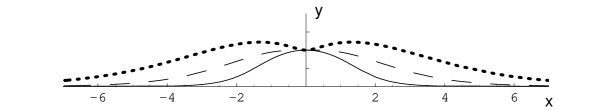
Figure 6.1: Curves $y=y(x)$ for three values of the winding number $n$: $n=0$ (solid line), $n=1$ (dashed curve) and $n=2$ (dotted line). These three curves correspond to $r_{*}=1$.

Let us pause for a moment to study the function (6.4.19). First of all it is easy to verify that this function is invariant if we change $n\rightarrow-n$ and $c\rightarrow 1/c$ (or equivalently changing $\theta\rightarrow\pi-\theta$ for the same constant $c$). Actually, in what follows we shall take the integration constant $c=1$ and thus we can restrict ourselves to the case in which $n$ is non-negative. In this $c=1$ case, $r_{*}$ is the minimal separation between the brane probe and the origin. Another observation is that $r$ diverges for $\theta=0,\pi$, which corresponds to the location of the spikes of the worldvolume solitons. Therefore the supersymmetric embedding we have found is non-compact. Actually, it has the topology of a cylinder whose compact direction is parametrized by $\varphi$. This cylinder connects the two poles at $\theta=0,\pi$ of the $(\theta,\varphi)$ sphere at $r=\infty$ and passes at a distance $r_{*}$ from the origin.

It is also interesting to discuss the symmetries of our solutions. Recall that the angle $\tilde{\psi}$ is constant for our embeddings. Thus, it is clear that one can shift it by an arbitrary constant $\epsilon$ as $\tilde{\psi}\rightarrow\tilde{\psi}+\epsilon$. This $U(1)$ symmetry corresponds to an isometry of the abelian background which is broken quantum-mechanically to ${\rm Z}\kern-3.8pt{\rm Z}\kern 2.0pt_{2N}$ as a consequence of the flux quantization of the RR two-form potential [37, 110, 48]. In the gauge theory side this isometry has been identified [37, 110, 48] with the $U(1)$ R-symmetry of the ${\cal N}=1$ SYM theory, which is broken down to ${\rm Z}\kern-3.8pt{\rm Z}\kern 2.0pt_{2N}$ by a field theory anomaly [109]. On the other hand, it is also clear that we have an additional $U(1)$ associated to constant shifts in $\tilde{\varphi}$, which are equivalent to a redefinition of $\varphi_{0}$ in eq. (6.4.16).

To visualize the shape of the brane in these solutions it is rather convenient to introduce the following cartesian coordinates $x$ and $y$ :

$$x\,=\,r\cos\theta\,\,,\,\,\,\,\,\,\,\,\,\,\,\,\,\,\,y\,=\,r\sin\theta\,\,.$$ (6.4.20)

In terms of $(x,y)$ the D5-brane embedding will be described by means of a curve $y=y(x)$. Notice that $y\geq 0$, whereas $-\infty<x<+\infty$. The value of the coordinate $y$ at $x=0$ is just $r_{*}$, i.e. $y(x=0)=r_{*}$. Moreover, for large values of the coordinate $x$, the function $y(x)\rightarrow 0$ exponentially as

$$y(x)\,\approx C\,|x|\,e^{-{2\over|n|+1}|x|}\,\,,\,\,\,\,\,\,\,\,\,\,\,\,\,\,\,(|x|\rightarrow\infty)\,\,,$$ (6.4.21)

where $C$ is a constant. To illustrate this behavior we have plotted in figure 6.1 the curves $y(x)$ for three different values of the winding $n$ and the same value of $r_{*}$.

A particularly interesting case is obtained when $n=\pm 1$. By adjusting properly the constant $\varphi_{0}$ in eq. (6.4.16), the angular embedding reduces to:

$$\tilde{\theta}\,=\,\theta\,\,,\,\,\,\,\,\,\,\,\,\,\,\,\,\,\tilde{\varphi}\,=\,\varphi\,+\,{\rm constant}\,\,,\,\,\,\,\,\,\,\,\,\,\,\,\,\,\,\,\,\,\,\,\,\,\,\,\,\,\,\,\,\,\,\,\,\,\,\,\,\,\,\,\,\,(n=1)\,\,,$$

$$\tilde{\theta}\,=\,\pi-\theta\,\,,\,\,\,\,\,\,\,\,\,\,\,\,\,\,\tilde{\varphi}\,=\,2\pi-\varphi\,+\,{\rm constant}\,\,,\,\,\,\,\,\,\,\,\,\,\,\,\,\,(n=-1)\,\,,$$ (6.4.22)

with $\tilde{\psi}$ being constant. These types of angular embeddings are similar to the ones considered in ref. [85] (although they are not the same, see eq. (6.3.20) ) and we will refer to them as unit-winding embeddings. Notice that the two cases displayed in eq. (6.4.22) represent the two possible identifications of the $(\theta,\varphi)$ and $(\tilde{\theta},\tilde{\varphi})$ two-spheres.

When $n=0$ the brane is wrapping the $(\theta,\varphi)$ sphere at constant values of $\tilde{\theta}$ and $\tilde{\varphi}$, i.e. one has:

$$\tilde{\theta}\,=\,{\rm constant}\,=\,\tilde{\theta}_{0}\,\,,\,\,\,\,\,\,\,\,\,\,\,\,\,\,\,\,\,\,\,\tilde{\varphi}\,=\,{\rm constant}\,=\,\tilde{\varphi}_{0}\,\,,\,\,\,\,\,\,\,\,\,\,\,\,\,\,\,\,\,\,\,(n=0)$$ (6.4.23)

We will refer to this case as zero-winding embedding [83].

One can verify that the brane embeddings we have found are solutions of the probe equations of motion. Actually, they are supersymmetric worldvolume solitons of the D5 brane probe. To illustrate this fact let us show that these configurations saturate a BPS energy bound. To simplify matters, let us assume that the angular embedding is the one displayed in eq. (6.4.16) and let $r(\theta)$ be an arbitrary function. The Dirac-Born-Infeld (DBI) lagrangian density for a D5-brane with unit tension is:

$${\cal L}\,=\,-e^{-\phi}\,\sqrt{-g_{st}}\,+\,P\,\Big{[}\,C_{(6)}\,\Big{]}\,\,,$$ (6.4.24)

where $g_{st}$ is the determinant of the induced metric in the string frame ($g_{st}=e^{3\phi}\,g$) and $P\,\Big{[}\,C_{(6)}\,\Big{]}$ is the pullback on the worldvolume of the RR six-form of the background. The elements of the induced metric for the $n$-winding solution along the angular coordinates are:

$$g_{\theta\theta} = e^{{\phi\over 2}}\,\bigg{(}\,e^{2h}\,+\,{n^{2}\over 4}\,{\sin^{2}\tilde{\theta}\over\sin^{2}\theta}\,+\,r_{\theta}^{2}\,\bigg{)}\,\,,$$ (6.4.25)

$$g_{\varphi\varphi} = e^{{\phi\over 2}}\,\bigg{(}\,e^{2h}\,+\,{n^{2}\over 4}\,{\sin^{2}\tilde{\theta}\over\sin^{2}\theta}\,+\,V_{3\varphi}^{2}\,\bigg{)}\sin^{2}\theta\,\,.$$ (6.4.27)

From this expression one immediately obtains the determinant of the induced metric, namely:

$$\sqrt{-g}\,=\,e^{{3\phi\over 2}}\,\sin\theta\,\,\sqrt{\bigg{(}\,e^{2h}\,+\,{n^{2}\over 4}\,{\sin^{2}\tilde{\theta}\over\sin^{2}\theta}\,+\,V_{3\varphi}^{2}\,\bigg{)}\,\bigg{(}\,e^{2h}\,+\,{n^{2}\over 4}\,{\sin^{2}\tilde{\theta}\over\sin^{2}\theta}\,+\,r_{\theta}^{2}\,\bigg{)}}\,\,.$$ (6.4.28)

Moreover, the pullback on the worldvolume of the two-form ${\cal C}$ is :

$$P\,\Big{[}\,{\cal C}\,\Big{]}\,=\,{e^{2\phi}\over 8}\,(\,16e^{2h}\,\cos\theta\,-\,ne^{-2h}\,\cos\tilde{\theta}\,)\,r_{\theta}\,d\varphi\wedge d\theta$$ (6.4.29)

The hamiltonian density ${\cal H}$ for a static configuration is just ${\cal H}\,=\,-{\cal L}$ or:

$${\cal H}\,=\,e^{2\phi}\,\Bigg{[}\,\sin\theta\,\sqrt{\bigg{(}\,e^{2h}\,+\,{n^{2}\over 4}\,{\sin^{2}\tilde{\theta}\over\sin^{2}\theta}\,+\,V_{3\varphi}^{2}\,\bigg{)}\,\bigg{(}\,e^{2h}\,+\,{n^{2}\over 4}\,{\sin^{2}\tilde{\theta}\over\sin^{2}\theta}\,+\,r_{\theta}^{2}\,\bigg{)}}\,-\,$$

$$\,\,\,\,\,\,\,\,\,\,\,\,\,\,\,\,\,\,\,\,-\,{1\over 8}\,(\,16e^{2h}\,\cos\theta\,-\,ne^{-2h}\,\cos\tilde{\theta}\,)\,r_{\theta}\,\Bigg{]}\,\,,$$ (6.4.30)

It can be checked that, for an arbitrary function $r(\theta)$, one can write ${\cal H}$ as:

$${\cal H}\,=\,{\cal Z}\,+\,{\cal S}\,\,,$$ (6.4.31)

where ${\cal Z}$ is a total derivative:

$${\cal Z}\,=\,-\partial_{\theta}\,\Bigg{[}\,e^{2\phi}\,\bigg{(}e^{2h}\,\cos\theta\,+\,{n\over 4}\,\cos\tilde{\theta}\,\bigg{)}\,\Bigg{]}\,\,,$$ (6.4.32)

and ${\cal S}$ is non-negative:

$${\cal S}\geq 0\,\,,$$ (6.4.33)

with ${\cal S}=0$ precisely when the BPS equations for the embedding are satisfied. The expression of ${\cal S}$ is:

$${\cal S} = \sin\theta\,e^{2\phi}\,\Bigg{[}\,\sqrt{\bigg{(}\,e^{2h}\,+\,{n^{2}\over 4}\,{\sin^{2}\tilde{\theta}\over\sin^{2}\theta}\,+\,V_{3\varphi}^{2}\,\bigg{)}\,\bigg{(}\,e^{2h}\,+\,{n^{2}\over 4}\,{\sin^{2}\tilde{\theta}\over\sin^{2}\theta}\,+\,r_{\theta}^{2}\,\bigg{)}}\,\,-$$ (6.4.34)

$$\,\,\,\,\,\,\,\,\,\,\,\,\,\,\,\,\,\,\,\,\,\,\,\,\,\,\,\,-\bigg{(}\,e^{2h}\,+\,{n^{2}\over 4}\,{\sin^{2}\tilde{\theta}\over\sin^{2}\theta}\,-\,V_{3\varphi}\,r_{\theta}\,\bigg{)}\,\Bigg{]}\,\,.$$

The BPS equation for $r$ in this case is $r_{\theta}=-V_{3\varphi}$ (see eq. (6.4.2)). If this equation is satisfied, the first term on the right-hand side of eq. (6.4.34) is a square root of a perfect square which cancels against the second term of this equation. Moreover, it is easy to check that the condition ${\cal S}\geq 0$ is equivalent to:

$$\big{(}r_{\theta}\,+\,V_{3\varphi}\,\big{)}^{2}\geq 0\,\,,$$ (6.4.35)

which is obviously satisfied and reduces to an equality if and only if the BPS equation for the embedding is satisfied.

6.4.2 (n,m)-Winding solitons

The solutions found in the previous section are easily generalized if we allow the angle $\tilde{\psi}$ to wind a certain number of times as the coordinate $\varphi$ varies from $\varphi=0$ to $\varphi=2\pi$. Recalling that $\tilde{\psi}$ ranges from $0$ to $4\pi$, let us write the following ansatz for $\tilde{\psi}(\varphi)$:

$$\tilde{\psi}\,=\,\tilde{\psi}_{0}\,+\,2m\varphi\,\,,$$ (6.4.36)

where $m$ is an integer. It is obvious that the above function satisfies the Laplace equation (6.4.10). Moreover, its harmonic conjugate $\Lambda$ is immediately obtained by solving the Cauchy-Riemann differential equations (6.4.12), namely:

$$\Lambda\,=\,-2mu\,\,.$$ (6.4.37)

In terms of the angle $\theta$, the above equation becomes:

$$e^{\Lambda}\,=\,{1\over\Big{(}\,\tan{\theta\over 2}\,\Big{)}^{2m}}\,\,.$$ (6.4.38)

By plugging this result in eq. (6.4.14), and using the value of $\sin\tilde{\theta}$ given in eq. (6.4.18), it is straightforward to obtain the function $r(\theta)$ of the embedding. One gets:

$$e^{2r}\,=\,{e^{2r_{*}}\over 1+c}\,\,{(\,1\,+\,\cos\theta\,)^{n}\,+\,c\,(\,1\,-\,\cos\theta\,)^{n}\over\big{[}\tan{\theta\over 2}\big{]}^{2m}(\sin\theta\,)^{n+1}}\,\,,$$ (6.4.39)

where, as in the $n$-winding case, $r_{*}=r(\theta=\pi/2)$.

An interesting observation concerning the solution we have just found is that, by choosing appropriately the winding number $m$, one of the spikes of the $m=0$ solutions at $\theta=0$ or $\theta=\pi$ disappears. Indeed if, for example, $n$ is non-negative and we take $2m=n+1$, the function $r(\theta)$ is regular at $\theta=0$. Similarly, also when $n\geq 0$, one can eliminate the spike at $\theta=\pi$ by choosing $2m=-n-1$.

6.4.3 Spiral solitons

By considering more general solutions of the Cauchy-Riemann equations (6.4.5) and (6.4.12) we can obtain many more classes of supersymmetric configurations of the brane probe. One of the questions one can address is whether or not one can have embeddings in which $r$ is finite for all values of the angles. We will now see that the answer to this question is yes, although the corresponding embeddings seem not to be very interesting. To illustrate this point, let us see how we can find functions $\tilde{\psi}$ and $\Lambda$ such that they make the radial coordinate of the $n$-winding embedding finite at $\theta=0,\pi$. First of all, notice that, in terms of the Cauchy-Riemann variables $u$ and $\tilde{u}$ defined in eq. (6.4.4), we have to explore the behavior of the embedding at $u,\tilde{u}\rightarrow\pm\infty$. Since:

$$\sin\theta\,=\,{2e^{u}\over 1+e^{2u}}\,\,,\,\,\,\,\,\,\,\,\,\,\,\,\,\,\,\,\,\,\,\,\,\sin\tilde{\theta}\,=\,{2e^{\tilde{u}}\over 1+e^{2\tilde{u}}}\,\,,$$ (6.4.40)

one has that $\sin\theta\rightarrow e^{-|u|}$, $\sin\tilde{\theta}\rightarrow e^{-|\tilde{u}|}$ as $u,\tilde{u}\rightarrow\pm\infty$. Then, the factors multiplying $e^{\Lambda}$ in eq. (6.4.14) diverge as $e^{|u|+|\tilde{u}|}$. In the $n$-winding solution $|\tilde{u}|=|n||u|$ and, therefore this divergence is of the type $e^{(|n|+1)|u|}$. We can cancel this divergence by adding a $\Lambda$ such that $e^{\Lambda}\rightarrow 0$ as $u\rightarrow\pm\infty$ in such a way that, for example, $\Lambda+(|n|+1)|u|\rightarrow-\infty$. This is clearly achieved by taking a function $\Lambda$ such that $\Lambda\rightarrow-u^{2}$. It is straightforward to find an analytic function in the $(u,\varphi)$ plane such that its imaginary part behaves as $-u^{2}$ for $u\rightarrow\pm\infty$. One can take

$$\tilde{\psi}+i\Lambda\,=\,-i(u+i\varphi)^{2}\,=\,2u\varphi\,-\,i(u^{2}-\varphi^{2})\,\,.$$ (6.4.41)

From this equation we can read the functions $\tilde{\psi}$ and $\Lambda$. In terms of $\theta$ and $\varphi$ they are:

$$\tilde{\psi}\,=\,2u\varphi\,=\,2\varphi\log\tan{\theta\over 2}\,\,,\,\,\,\,\,\,\,\,\,\,\,\,\,\,\,\,\,\,\,\,\,\Lambda\,=\,-u^{2}+\varphi^{2}\,=\,-\big{(}\,\log\tan{\theta\over 2}\,\big{)}^{2}\,+\,\varphi^{2}\,\,.$$ (6.4.42)

In this case $r\rightarrow 0$, $\tilde{\psi}\rightarrow\pm\infty$ as $\theta\rightarrow 0,\pi$, which means that we describe an infinite spiral which winds infinitely in the $\tilde{\psi}$ direction. Notice that, although $r$ is always finite, the volume of the two-submanifold is infinite due to this infinite winding. One can try other alternatives to make the radial coordinate finite. In all the ones we have analyzed, one obtains the infinite spiral behavior described above.

6.5 Worldvolume solitons (non-abelian case)

Let us consider the full non-abelian background and let us try to obtain solutions to the kappa symmetry equations (6.2.9)-(6.2.13). Actually we will restrict ourselves to the situations in which $r$ only depends on the angle $\theta$. It can be easily checked that, in this case, only four of the five equations (6.2.9)-(6.2.13) are independent. As an independent set of equations we will choose eqs. (6.2.9), (6.2.17) and:

$$\partial_{\theta}r=-{e^{h}\,V_{3\varphi}\over e^{h}\,\cos\alpha\,+\,(\,V_{2\varphi}\,-\,{a\over 2}\,)\,\sin\alpha}\,\,,$$ (6.5.1)

$$\sin\alpha V_{1\varphi}\,\partial_{\theta}r\,-\,e^{h}\,V_{3\theta}=0\,\,,$$ (6.5.2)

which can be obtained from eqs. (6.2.10) and (6.2.13) after taking $\partial_{\varphi}r=0$.

We will now try to find the non-abelian version of the solutions found in the abelian theory for arbitrary winding $n$. With this purpose, let us consider the following ansatz for $\tilde{\varphi}$:

$$\tilde{\varphi}(\theta,\varphi)\,=\,n\varphi\,+\,f(\theta)\,\,,$$ (6.5.3)

while we shall assume that $\tilde{\theta}$, $\tilde{\psi}$ and $r$ are functions of $\theta$ only. We will require that, in the asymptotic UV, $\tilde{\varphi}\rightarrow n\varphi$. It is clear that in this ansatz $\partial_{\varphi}\tilde{\varphi}\,=\,n$ and that $\partial_{\theta}\tilde{\varphi}\,=\,\partial_{\theta}f$. Moreover, from eq. (6.2.9) we can obtain the relation between $\partial_{\theta}\tilde{\varphi}$ and $\partial_{\theta}\tilde{\theta}$, namely:

$$\partial_{\theta}\tilde{\varphi}\,=\,\tan\tilde{\psi}\,\,\bigg{[}\,{\partial_{\theta}\tilde{\theta}\over\sin\tilde{\theta}}\,-\,{n\over\sin\theta}\,\bigg{]}\,\,.$$ (6.5.4)

Using this value of $\partial_{\theta}\tilde{\varphi}$, we get the following values of the $V$ functions:

$$V_{1\theta}\,=\,{1\over 2}\,\bigg{[}\,{\partial_{\theta}\tilde{\theta}\over\cos\tilde{\psi}}\,-\,n\,{\sin\tilde{\theta}\over\sin\theta}\,\,{\sin^{2}\tilde{\psi}\over\cos\tilde{\psi}}\,\bigg{]}\,\,,$$

$$V_{1\varphi}\,=\,{n\over 2}\,{\sin\tilde{\theta}\over\sin\theta}\,\sin\tilde{\psi}\,=\,-V_{2\theta}\,\,,$$

$$V_{2\varphi}\,=\,{n\over 2}\,{\sin\tilde{\theta}\over\sin\theta}\,\cos\tilde{\psi}\,\,,$$

$$V_{3\theta}\,=\,{1\over 2}\,\partial_{\theta}\tilde{\psi}\,+\,{1\over 2}\,\cot\tilde{\theta}\,\tan\tilde{\psi}\,\partial_{\theta}\tilde{\theta}\,-\,{n\over 2}\,\tan\tilde{\psi}\,{\cos\tilde{\theta}\over\sin\theta}\,\,,$$

$$V_{3\varphi}\,=\,{n\over 2}\,{\cos\tilde{\theta}\over\sin\theta}\,+\,{1\over 2}\,\cot\theta\,\,.$$ (6.5.5)

By using these values in eq. (6.2.17), one gets the value of $\partial_{\theta}\tilde{\theta}$ in terms of the other variables:

$$\partial_{\theta}\tilde{\theta}\,=\,{n\sin\tilde{\theta}\cosh 2r-\sin\theta\cos\tilde{\psi}\over\sin\theta\cosh 2r-n\sin\tilde{\theta}\cos\tilde{\psi}}\,\,.$$ (6.5.6)

On the other hand, by combining the two equations (6.5.4) and (6.5.6), we obtain:

$$\partial_{\theta}\,\tilde{\varphi}\,=\,{n^{2}\sin^{2}\tilde{\theta}\,-\,\sin^{2}\theta\over\sin\theta\sin\tilde{\theta}\,(\,\sin\theta\cosh 2r\,-\,n\sin\tilde{\theta}\cos\tilde{\psi}\,)}\,\sin\tilde{\psi}\,\,.$$ (6.5.7)

Moreover, plugging the values of $V_{1\varphi}$, $V_{2\varphi}$, $V_{3\theta}$ and $V_{3\varphi}$ in eqs. (6.5.1) and (6.5.2) we can obtain the values of the derivatives of $\tilde{\psi}$ and $r$. The result is:

$$\partial_{\theta}\tilde{\psi} = {n\cot\theta\sin\tilde{\theta}+\cot\tilde{\theta}\sin\theta\over\sin\theta\cosh 2r-n\sin\tilde{\theta}\cos\tilde{\psi}}\,\,\sin\tilde{\psi}\,\,,$$

$$\partial_{\theta}r = -{1\over 2}\,\,{n\cos\tilde{\theta}+\cos\theta\over\sin\theta\cosh 2r-n\sin\tilde{\theta}\cos\tilde{\psi}}\,\,\sinh 2r\,\,.$$ (6.5.8)

It follows from eq. (6.5.6) that, asymptotically in the UV, $\sin\theta\,\partial_{\theta}\tilde{\theta}\rightarrow n\sin\tilde{\theta}$. If one wants to fulfil this relation for arbitrary $r$ it is easy to see from eq. (6.5.6) that one must have $(n\sin\tilde{\theta})^{2}=\sin^{2}\theta$, which only happens for $n=\pm 1$ and $\sin\theta=\sin\tilde{\theta}$. Noticing that for these values one has $\partial_{\theta}\tilde{\theta}\,=\,\pm 1$, one is finally led to the two possibilities of eq. (6.4.22): $\tilde{\theta}=\theta$ for $n=1$ and $\tilde{\theta}=\pi-\theta$ for $n=-1$. Notice that in the two cases of eq. (6.4.22) this equation implies that $\partial_{\theta}\,\tilde{\varphi}=0$ and thus when $n=\pm 1$ the angular identifications of the abelian unit-winding embeddings (eq. (6.4.22)) also solve the non-abelian equations (6.5.6) and (6.5.7) for all $r$.

For a general value of $n$, one has that asymptotically in the UV $\partial_{\theta}\tilde{\varphi}\rightarrow 0$ and $\partial_{\theta}\tilde{\psi}\rightarrow 0$, as in the abelian solutions. Moreover it follows from eqs. (6.5.7) and (6.5.8) that $\tilde{\varphi}$ and $\tilde{\psi}$ can be kept constant for all $r$ if $\sin\tilde{\psi}=0$, i.e. when $\tilde{\psi}=0,\pi\,\,\,{\hbox{\rm mod}}\,\,2\pi$. For these values of $\tilde{\psi}$ the equations simplify and, although we will not attempt to do it here, one could try to integrate numerically the equations of $\tilde{\theta}$ and $r$. It is however interesting to point out that, contrary to what happens in the abelian $n$-winding solution, the angle $\tilde{\psi}$ cannot be an arbitrary constant for the non-abelian probes. As we will argue below, this is a geometrical realization of the breaking of the R-symmetry of the corresponding ${\cal N}=1$ SYM theory in the IR. On the contrary, the angle $\tilde{\varphi}$ can take an arbitrary constant value, as in the abelian solution.

6.5.1 Non-abelian unit-winding solutions

Let us now obtain the non-abelian generalization of the unit-winding solutions. First of all we define:

$$\eta\,=\,n=\pm 1\,\,.$$ (6.5.9)

We have already noticed that for unit-winding embeddings the values of $\tilde{\theta}$ and $\tilde{\varphi}$ displayed in eq. (6.4.22) solve the non-abelian differential equations (6.5.6) and (6.5.7). Therefore, let us try to find a solution in the non-abelian theory in which the embedding of the $(\tilde{\theta},\tilde{\varphi})$ coordinates is the same as in the abelian theory, i.e. as in eq. (6.4.22). For this type of embeddings $\sin\tilde{\theta}=\sin\theta$, $\partial_{\theta}\tilde{\theta}\,=\,\eta$ and eq. (6.5.5) reduces to:

$$V_{1\theta}\,=\,{\eta\cos\tilde{\psi}\over 2}\,\,,\,\,\,\,\,\,\,\,\,\,\,\,\,\,\,\,\,\,\,\,\,\,\,\,\,\,V_{1\varphi}\,=\,{\eta\sin\tilde{\psi}\over 2}\,\,,$$

$$V_{2\theta}\,=\,-{\eta\sin\tilde{\psi}\over 2}\,\,,\,\,\,\,\,\,\,\,\,\,\,\,\,\,\,\,\,\,\,\,\,\,V_{2\varphi}\,=\,{\eta\cos\tilde{\psi}\over 2}\,\,,$$

$$V_{3\theta}\,=\,{\tilde{\psi}_{\theta}\over 2}\,\,,\,\,\,\,\,\,\,\,\,\,\,\,\,\,\,\,\,\,\,\,\,\,\,\,\,\,\,\,\,\,\,\,\,\,\,\,\,\,V_{3\varphi}\,=\,\cot\theta\,\,,$$ (6.5.10)

where we have denoted $\tilde{\psi}_{\theta}\equiv\partial_{\theta}\,\tilde{\psi}$. As a check, notice that $V_{1\theta}$, $V_{1\varphi}$, $V_{2\theta}$ and $V_{2\varphi}$ satisfy eqs. (6.4.1). It follows from eq. (6.2.17) that they must also satisfy:

$$V_{1\theta}^{2}\,+\,V_{1\varphi}^{2}\,=\,{1\over 4}\,\,,\,\,\,\,\,\,\,\,\,\,\,\,\,\,\,\,\,\,\,\,\,\,V_{2\theta}^{2}\,+\,V_{2\varphi}^{2}\,=\,{1\over 4}\,\,,$$ (6.5.11)

which indeed they verify. Moreover, by substituting $\sin\tilde{\theta}=\sin\theta$ and $\cos\tilde{\theta}=\eta\cos\theta$ in eq. (6.5.8), we obtain the following differential equations for $\tilde{\psi}(\theta)$ and $r(\theta)$:

$$\tilde{\psi}_{\theta} = -{2\eta\sin\tilde{\psi}\over\sinh 2r}\,\,r_{\theta}\,\,,$$

$$r_{\theta} = -{\cot\theta\over\cosh 2r\,-\,\eta\cos\tilde{\psi}}\,\,\sinh 2r\,\,.$$ (6.5.12)

These equations can be integrated with the result:

$$\Bigg{(}\,\tan\,{\tilde{\psi}\over 2}\,\Bigg{)}^{\eta}\,=\,A\,\coth r\,\,,$$

$${\sinh r\over\sqrt{A^{2}+\tanh^{2}r}}\,=\,{C\over\sin\theta}\,\,,$$ (6.5.13)

where $A$ and $C$ are constants of integration. Eq. (6.5.13), together with eq. (6.4.22), determines the unit-winding embeddings of the probe in the non-abelian background. Notice that, as in the corresponding abelian solution, $r$ diverges when $\theta=0,\pi$, i.e.  the brane probe extends infinitely in the radial direction. On the other hand, it is also instructive to explore the $r\rightarrow\infty$ limit of the solution (6.5.13). First of all, it is clear that when $r\rightarrow\infty$ the angle $\tilde{\psi}$ reaches asymptotically a constant value $\tilde{\psi}_{0}$, given by:

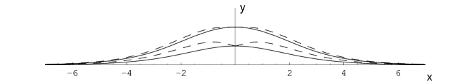
Figure 6.2: Comparison between the non-abelian (solid line) and abelian (dashed line) unit-winding embeddings for the same value of $r_{*}$ . The non-abelian embedding is the one corresponding to eq. (6.5.15) and the abelian one is that given in eq. (6.4.19) for $n=1$ and $c=1$. The curves for two different values of $r_{*}$ ($r_{*}=0.5$ and $r_{*}=1$) are shown. The variables $(x,y)$ are the ones defined in eq. (6.4.20).

$$\cos\tilde{\psi}_{0}\,=\,{1-A^{2}\over 1+A^{2}}\,\,\eta\,\,.$$ (6.5.14)

Moreover, when $r\rightarrow\infty$, the function $r(\theta)$ displayed in eq. (6.5.13) becomes, after a proper identification of the integration constants, exactly the one written in eq. (6.4.19) for $n=\pm 1$ and $c=1$. Notice that the angle $\tilde{\psi}$ in the embedding (6.5.13) is not constant in general. Actually, only when $A=0$ or $A=\infty$ the coordinate $\tilde{\psi}$ remains constant and equal to $0,\pi\,\,{\hbox{\rm mod}}\,2\pi$ ($\cos\tilde{\psi}=\eta$ for $A=0$ and $\cos\tilde{\psi}=-\eta$ in the case $A=\infty$). It is interesting to write the dependence of $r$ on $\theta$ in these two particular cases. When $A=\infty$ the solution is:

$$\tilde{\theta} = \cases{\theta,&if $\,\,\eta=+1\,,$\cr\pi-\theta,&if $\,\,\eta=-1\,,$}\,\,,\,\,\,\,\,\,\,\,\,\,\,\,\tilde{\varphi}\,=\,\cases{\varphi+{\rm constant},&if $\,\,\eta=+1\,,$\cr 2\pi-\varphi+{\rm constant},&if $\,\,\eta=-1$}\,\,,$$

$$\tilde{\psi} = \cases{\pi,3\pi,&if $\,\,\eta=+1\,,$\cr 0,2\pi,&if $\,\,\eta=-1\,,$}\,\,,\,\,\,\,\,\,\,\,\,\,\,\,\sinh r\,=\,{\sinh r_{*}\over\sin\theta}\,\,\,,$$ (6.5.15)

where $r_{*}$ is the minimal value of $r$ (i.e. $r_{*}=r(\theta=\pi/2)$) and we have also displayed the angular part of the embedding. Notice that, for a given sign of the winding number $\eta$, only two values of $\tilde{\psi}$ are possible. Thus, in this solution, the $U(1)$ symmetry of shifts in $\tilde{\psi}$ is broken to a ${\rm Z}\kern-3.8pt{\rm Z}\kern 2.0pt_{2}$ symmetry. This will be interpreted in section 6.6 as the realization, at the level of the brane probe, of the R-symmetry breaking of the gauge theory.

To have a better understanding of the solution (6.5.15) we have plotted it in figure 6.2 in terms of the variables $(x,y)$ defined in eq. (6.4.20). For comparison we have also plotted the abelian solution corresponding to the same value of $r_{*}$. In this figure the embeddings for two different values of the minimal radial distance $r_{*}$ are shown. When $r_{*}$ is large enough ($r_{*}\geq 2$) the two curves become practically identical.

In figure 6.3, a pictorial representation of the non-abelian unit-winding embedding of the brane has been plotted. $r_{*}$ is the minimal distance to the origin it reaches. From the five-dimensional point of view, we see how the brane vanishes in thin air at $r=r_{*}$, while it is space-time filling as it goes to $r\rightarrow\infty$. For $r_{*}=0$, we have the cylinder solutions described below. This limit is somehow pathological as the brane gets disconnected into two pieces, one at $\theta=\tilde{\theta}=0$ (suppose $\eta=+1$) and the other at $\theta=\tilde{\theta}=\pi$ without going through intermediate values of $\theta$.

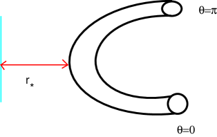
Figure 6.3: A pictorial representation of the embedding, which has the topology of a cylinder. The compact direction is the $\varphi$ angle, while the non-compact one extends in $r(\theta)$. It goes to infinity for $\theta=0,\pi$ and $r$ is minimum for $\theta=\pi/2$. Besides, the probe brane is also extended in the four flat space-time dimensions where the gauge theory lives.

Let us now have a look at the case of the $A=0$ embeddings. The function $r(\theta)$ in this case can be read from eq. (6.5.13), namely:

$$\cosh r\,=\,{C\over\sin\theta}\,\,\,.$$ (6.5.16)

We have plotted in figure 6.4 the profile for these embeddings in terms of the variables $(x,y)$ of eq. (6.4.20). Notice that, when $C$ is in the interval $(1,\infty)$ it can be parametrized as $C=\cosh r_{*}$, with $r_{*}>0$ being the minimal radial distance between the probe and the origin. On the contrary, when $C$ lies in the interval $[0,1]$ the brane reaches the origin when $\sin\theta=C$. We have thus, in this case, a one-parameter family of configurations which pass through the origin.

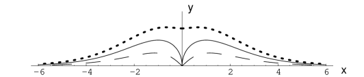
Figure 6.4: Graphic representation of the unit winding embedding of eq. (6.5.16) for three values of the constant $C$: $C=0.5$ (dashed line), $C=1$ (solid line) and $C=1.5$ (dotted line). The variables $(x,y)$ are the ones defined in eq. (6.4.20).

As in their abelian counterparts, all of these worldvolume solitons for the non-abelian background saturate an energy bound. In order to prove this fact, let us define:

$$D\,\equiv\,\coth 2r\,-\,\eta\,{\cos\tilde{\psi}\over\sinh 2r}\,\,.$$ (6.5.17)

Notice that $D\geq 0$ for any real $\tilde{\psi}$ and $r$. Moreover the equation for $r(\theta)$ can be written as $r_{\theta}=-\cot\theta/D$. For arbitrary functions $r(\theta)$ and $\tilde{\psi}(\theta)$ the hamiltonian density takes the form:

$${\cal H}\,=\,e^{2\phi}\sin\theta \Bigg{[} \sqrt{\Big{(}r-r_{\theta}\cot\theta\Big{)}^{2}\,+\,rD\,\Big{(}r_{\theta}+{\cot\theta\over D}\,\Big{)}^{2}\,+\,{rD\over 4}\Big{(}\tilde{\psi}_{\theta}\,-\,{2\eta\sin\tilde{\psi}\over D\sinh 2r}\,\cot\theta\,\Big{)}^{2}}\,-$$ (6.5.18)

$$-\,\Big{(}\,2e^{2h}\,-\,{1\over 8}\,(a^{2}-1)^{2}\,e^{-2h}\,\,\Big{)}\,\cot\theta\,\,r_{\theta}\Bigg{]}\,\,.$$

It can be verified that ${\cal H}$ can be written as ${\cal H}={\cal Z}+{\cal S}$, where:

$${\cal Z}=-{d\over d\theta}\,\Big{[}\,e^{2\phi}\,r\cos\theta\,\Big{]}\,\,.$$ (6.5.19)

(this is the same value as in the abelian soliton for $n=1$). The expression of ${\cal S}$ is:

$${\cal S}\,=\,e^{2\phi}\sin\theta \Bigg{[} \sqrt{\Big{(}r-r_{\theta}\cot\theta\Big{)}^{2}\,+\,rD\,\Big{(}r_{\theta}+{\cot\theta\over D}\,\Big{)}^{2}\,+\,{rD\over 4}\Big{(}\tilde{\psi}_{\theta}\,-\,{2\eta\sin\tilde{\psi}\over D\sinh 2r}\,\cot\theta\,\Big{)}^{2}}\,-$$ (6.5.20)

$$\,-\Big{(}\,r\,-\,r_{\theta}\cot\theta\,\big{)}\,\Bigg{]}\,\,.$$

As in the abelian case, if the BPS equations (6.5.12) are satisfied, the square root on eq. (6.5.20) can be exactly evaluated and ${\cal S}$ vanishes. Furthermore, one can easily check that ${\cal S}\geq 0$ is equivalent to the condition:

$$rD\,\Big{(}r_{\theta}+{\cot\theta\over D}\,\Big{)}^{2}\,+\,{rD\over 4}\Big{(}\tilde{\psi}_{\theta}\,-\,{2\eta\sin\tilde{\psi}\over D\sinh 2r}\,\cot\theta\,\Big{)}^{2}\,\geq\,0\,\,,$$ (6.5.21)

which, since $D\geq 0$, is trivially satisfied for any functions $r(\theta)$ and $\tilde{\psi}(\theta)$. Moreover, as $r-r_{\theta}\cot\theta\geq 0$ for the solution of the BPS equations, it follows that our BPS embedding saturates the bound.

6.5.2 Non-abelian zero-winding solutions

The differential equations for the non-abelian version of the zero-winding solution can be obtained by putting $n=0$ in our general equations. Actually, by taking $n=0$ in the second equation in (6.5.8) one obtains the differential equation which determines the dependence of $r$ on the angle $\theta$, namely:

$$r_{\theta}\,=\,-{\cot\theta\over 2\coth 2r}\,\,,$$ (6.5.22)

which can be easily integrated, namely:

$$\sinh 2r\,=\,{C\over\sin\theta}\,\,.$$ (6.5.23)

Notice that, as in the abelian case, this solution has two spikes at $\theta=0,\pi$, where $r$ diverges and, thus, the brane probe also extends infinitely in the radial direction. Moreover, the minimal value of the radial coordinate, which we will denote by $r_{*}$, is reached at $\theta=\pi/2$. This minimal value is related to the constant $C$ in eq. (6.5.23), namely $\sinh 2r_{*}=C$. It is readily verified that for large $r$ this solution behaves exactly as the zero-winding solution in the abelian theory. Moreover, it follows from eq. (6.5.4) that, in this $n=0$ case, the angle $\tilde{\varphi}$ only depends on $\theta$. Actually, the differential equations for the angles $\tilde{\theta}$, $\tilde{\varphi}$ and $\tilde{\psi}$ as functions of $\theta$ are easily obtained from eqs. (6.5.6), (6.5.7) and (6.5.4):

$$\partial_{\theta}\,\tilde{\theta} = -{\cos\tilde{\psi}\over\cosh 2r}\,\,,$$

$$\partial_{\theta}\,\tilde{\varphi} = -{1\over\cosh 2r}\,\,{\sin\tilde{\psi}\over\sin\tilde{\theta}}\,\,,$$

$$\partial_{\theta}\,\tilde{\psi} = {\cot\tilde{\theta}\sin\tilde{\psi}\over\cosh 2r}\,\,.$$ (6.5.24)

By combining the equations of $\tilde{\psi}$ and $\tilde{\theta}$ one can easily get the relation between these two angles, namely:

$$\sin\tilde{\psi}\,=\,{B\over\sin\tilde{\theta}}\,\,.$$ (6.5.25)

Notice that, for consistency, $B\leq 1$ and $\sin\tilde{\theta}\geq B$. We can also obtain $\tilde{\varphi}=\tilde{\varphi}(\tilde{\theta})$ and $\tilde{\theta}=\tilde{\theta}(\theta)$:

$$\tilde{\varphi}=-\arctan\Bigg{[}\,{B\cos\tilde{\theta}\over\sqrt{\sin^{2}\tilde{\theta}-B^{2}}}\Bigg{]}\,+\,{\rm constant}\,\,,$$

$$-\arcsin\Bigg{[}\,{\cos\tilde{\theta}\over\sqrt{1-B^{2}}}\Bigg{]}=\arcsin\Bigg{[}\,{\cos\theta\over\sqrt{1+C^{2}}}\Bigg{]}\,+\,{\rm constant}\,\,.$$ (6.5.26)

Actually, much simpler equations for the embedding are obtained if one considers the particular case in which the angle $\tilde{\psi}$ is constant. Notice that, as was pointed out after eq. (6.5.8), this only can happen if $\tilde{\psi}=0,\pi$ (${\hbox{\rm mod}}\,\,2\pi$) (see also the last equation in (6.5.24)). These solutions correspond to taking the constant $B$ equal to zero in eq. (6.5.25). Moreover, it follows from the eq. (6.5.24) that $\tilde{\varphi}$ is an arbitrary constant in this case, while the dependence of $\tilde{\theta}$ on $\theta$ can be obtained by combining eqs. (6.5.23) and (6.5.24). If we denote $\cos\tilde{\psi}=\epsilon$, with $\epsilon=\pm 1$, one has:

$$\sinh 2r\,=\,{\sinh 2r_{*}\over\sin\theta}\,\,,\,\,\,\,\,\,\,\,\,\,\,\,\,\,\,\,\,\,\,\sin(\,\tilde{\theta}\,-\,\tilde{\theta}_{*}\,)\,=\,\epsilon\,{\cos\theta\over\cosh 2r_{*}}\,\,,$$ (6.5.27)

where $\tilde{\theta}_{*}=\tilde{\theta}(\theta=\pi/2)$. Notice that there are four possible values of $\tilde{\psi}$ in this zero-winding solution and, thus, the $U(1)$ R-symmetry is broken to ${\rm Z}\kern-3.8pt{\rm Z}\kern 2.0pt_{4}$ in this case.

Let us finally point out that, also in this case, the hamiltonian density ${\cal H}$ can be put as ${\cal H}={\cal Z}+{\cal S}$, where ${\cal S}$ is non-negative (${\cal S}=0$ for the BPS solution) and ${\cal Z}$ is given by:

$${\cal Z}\,=\,-\partial_{\theta}\,\Bigg{[}\,e^{2\phi}\,\cos\theta\bigg{(}\,r\,-\,{1\over 4}\,\coth 2r\,+\,{r\over 2\sinh^{2}2r}\,\bigg{)}\,\Bigg{]}\,\,.$$ (6.5.28)

6.5.3 Cylinder solutions

We shall now show that there exists a general class of supersymmetric embeddings for the non-abelian background. For convenience, let us consider $r$ as worldvolume coordinate and let us assume that the D5-brane is sitting at the north poles of the $(\theta,\varphi)$ and $(\tilde{\theta},\tilde{\varphi})$ two-spheres, i.e. at $\theta=\tilde{\theta}=0$. In the remaining angular coordinates $\varphi$, $\tilde{\varphi}$ and $\tilde{\psi}$, the embedding is characterized by the equation:

$${\varphi-\varphi_{0}\over p}\,=\,{\tilde{\varphi}-\tilde{\varphi}_{0}\over q}\,=\,{\tilde{\psi}-\tilde{\psi}_{0}\over s}\,\,,$$ (6.5.29)

where $(\varphi_{0},\tilde{\varphi}_{0},\tilde{\psi}_{0})$ and $(p,q,s)$ are constants. Notice that, if one of the constants of the denominator in (6.5.29) is zero, then the corresponding angle must be a constant. Let us parametrize these embeddings by means of two worldvolume coordinates $\sigma_{1}$ and $\sigma_{2}$, defined as follows:

$$\sigma_{1}\,=\,{\varphi-\varphi_{0}\over p}\,=\,{\tilde{\varphi}-\tilde{\varphi}_{0}\over q}\,=\,{\tilde{\psi}-\tilde{\psi}_{0}\over s}\,\,,\,\,\,\,\,\,\,\,\,\,\,\,\,\,\,\,\,\sigma_{2}\,=\,r\,\,.$$ (6.5.30)

It is straightforward to demonstrate that the pullback to the worldvolume of the forms $w^{i}$ and $A^{i}$ is given by:

$$P[\,w^{1}\,]\,=\,P[\,w^{2}\,]\,=\,0\,\,,\,\,\,\,\,\,\,\,\,\,\,\,\,\,\,\,\,P[\,w^{3}\,]\,=\,(q+s)\,d\sigma_{1}\,\,,$$

$$P[\,A^{1}\,]\,=\,P[\,A^{2}\,]\,=\,0\,\,,\,\,\,\,\,\,\,\,\,\,\,\,\,\,\,\,\,P[\,A^{3}\,]\,=\,-p\,d\sigma_{1}\,\,.$$ (6.5.31)

It follows from these results that the pullback of the frame one-forms $e^{i}$ and $e^{\hat{j}}$ is zero for $i,j=1,2$, whereas $P[e^{\hat{3}}]$ is non-vanishing. As a consequence, the induced Dirac matrices are:

$$\gamma_{\sigma_{1}}\,=\,{1\over 2}\,(p+q+s)\,e^{{\phi\over 4}}\,\hat{\Gamma}_{3}\,\,,\,\,\,\,\,\,\,\,\,\,\,\,\,\,\,\,\,\,\,\,\,\,\,\,\,\,\,\,\,\,\,\,\,\,\gamma_{\sigma_{2}}\,=\,e^{{\phi\over 4}}\,\,\Gamma_{r}\,\,.$$ (6.5.32)

The kappa symmetry matrix $\Gamma_{\kappa}$ for the embedding at hand is:

$$\Gamma_{\kappa}\,=\,{e^{\phi}\over\sqrt{-g}}\,\Gamma_{x^{0}\cdots x^{3}}\,\gamma_{\sigma_{1}\sigma_{2}}\,\,.$$ (6.5.33)

Moreover, by using the projection conditions satisfied by the Killing spinors $\epsilon$, one can prove that:

$$\gamma_{\sigma_{1}\sigma_{2}}\,\epsilon\,=\,-{p+q+s\over 2}\,\,e^{{\phi\over 2}}\,\,\Gamma_{r}\,\hat{\Gamma}_{3}\,\epsilon\,=\,{p+q+s\over 2}\,\,e^{{\phi\over 2}}\,\Big{(}\,\cos\alpha\,\Gamma_{12}\,+\,\sin\alpha\Gamma_{1}\hat{\Gamma}_{2}\,\Big{)}\,\epsilon\,\,,$$ (6.5.34)

and, since the determinant of the induced metric is $\sqrt{-g}\,=\,e^{{3\phi\over 2}}\,{p+q+s\over 2}$, it is immediate to verify that the kappa symmetry projection $\Gamma_{\kappa}\epsilon=\epsilon$ coincides with the projection satisfied by the Killing spinors of the background. Therefore, our brane probe preserves all the supersymmetries of the background. Notice that the induced metric on the worldvolume along the $\sigma_{1},\sigma_{2}$ directions has the form

$$e^{{\phi\over 2}}\big{[}\,{(p+q+s)^{2}\over 4}\,d\sigma_{1}^{2}\,+\,d\sigma_{2}^{2}\,\big{]}\,\,,$$ (6.5.35)

which is conformally equivalent to the metric of a cylinder. After a simple calculation one can prove that the energy density of these solutions is

$${\cal H}\,=\,\partial_{r}\,\Bigg{[}\,e^{2\phi}\,\bigg{(}\,pr\,+\,(q+s-p)\,\bigg{(}{\coth 2r\over 4}\,-\,{r\over 2\sinh^{2}2r}\,\bigg{)}\,\bigg{)}\,\Bigg{]}\,\,.$$ (6.5.36)

One can also have cylinders located at the south pole of the $(\theta,\varphi)$ and $(\tilde{\theta},\tilde{\varphi})$ two-spheres. Indeed, the above equations remain valid if $\theta=\pi$ ($\tilde{\theta}=\pi$) if one changes $p\rightarrow-p$ ($q\rightarrow-q$, respectively). On the other hand, if $p=0$ , the angle $\varphi$ is constant and, as the pullback of the $e^{i}$ frame one-forms also vanishes when $\theta$ is also constant, it follows that $\theta$ can have any constant value when $p=0$. Similarly, if $q=0$ one necessarily has $\tilde{\varphi}=\tilde{\varphi}_{0}$ and $\tilde{\theta}$ can be an arbitrary constant in this case.

When $p=1$, $q=n$ and $s=2m$, the angular part of the embedding is the same as in the $(n,m)$-winding solitons. Actually, these cylinder solutions correspond to formally taking $r_{*}\rightarrow-\infty$ is the abelian solution of eq. (6.4.39). This forces one to take $\theta=0,\pi$ and, thus one can regard the cylinder as a zoom which magnifies the region in which the probe goes to infinity. One can also get cylinder embeddings by consider the limit of the non-abelian solutions in which the probe reaches the point $r=0$. For example, by taking $r_{*}=0$ in eq. (6.5.15) one gets the $p=q=1$, $s=0$ cylinder solutions while the $r_{*}\rightarrow 0$ limit of the embedding (6.5.27) corresponds to a cylinder with $p=1$ and $q=s=0$. Actually, when one takes the $r_{*}\rightarrow 0$ limit of these non-abelian embeddings one obtains two cylinder solutions, one with $\theta=0$ and the other with $\theta=\pi$. This suggests that, in order to obtain a consistent solution, one must combine in general two cylinders located at each of the two poles of the $(\theta,\varphi)$ two-sphere. Notice that this is also required if one imposes the condition of RR charge neutrality of the two-sphere at infinity.

6.6 Quadratic fluctuations around the unit-winding embedding

As mentioned in the introduction, we are now going to consider some of the brane probe configurations previously found as flavor branes, which will allow us to introduce dynamical quarks in the ${\cal N}=1$ SYM theory. Following refs. [98, 103, 104], the spectrum of quadratic fluctuations of the brane probe will be interpreted as the meson spectrum of ${\cal N}=1$ SQCD. So, let us try to elaborate on the reasons to consider these probes as the addition of flavors to the field theory dual. In fact, when considering the ’t Hooft expansion for large number of colors, the rôle of flavors is played by the boundaries of the Feynman graph. From a gravity perspective, these boundaries correspond to the addition of D-branes and open strings in the game.

In our case, we have a system of $N$ D5-branes wrapping a two-cycle inside the resolved conifold and $N_{f}$ D5-branes that wrap another two-submanifold, thus introducing $N_{f}$ flavors in the $SU(N)$ gauge theory. Taking the decoupling limit with $g_{s}\alpha^{\prime}N$ fixed and large is equivalent to replacing the $N$ D5-branes by the geometry they generate (the one studied in section 5.1.2), while the $N_{f}$-D5 branes that do not backreact (because we take $N_{f}$ much smaller than $N$) are treated as probes. From a gauge theory perspective, this is equivalent to consider the dynamics of gluons and gluinos coupled to fundamentals, but neglecting the backreaction of the latter. Of course it would be of great interest to find the backreacted solution.

The way of adding fundamental fields in this gauge theory from a string theory perspective was discussed in [99], where two possible ways, adding $D9$ branes or adding $D5$ branes as probes, were proposed. Here, we are considering the cleaner case of $D5$ probes. A careful analysis of the open string spectrum shows the existence of a four dimensional gauge ${\cal N}=1$ vector multiplet and a complex scalar multiplet. This is the spectrum of SQCD. In the case analyzed below we will consider abelian DBI actions for the probes, so that we will be dealing with the $N_{f}=1$ case.

We have found several brane configurations in the non-abelian background which, in principle, could be suitable to generate the meson spectrum. One of the requirements we should demand to these configurations is that they must incorporate some scale parameter which could be used to generate the mass scale of the quarks. Within our framework such a mass scale is nothing but the minimal distance between the flavor brane and the origin, i.e. what we have denoted by $r_{*}$. This requirement allows to discard the cylinder solutions we have found since they reach the origin and have no such a mass scale. We are thus left with the unit-winding solutions and the zero-winding solutions of section 6.5 as the only analytical solutions we have found for the non-abelian background.

In this section we shall analyze the fluctuations around the unit-winding solutions. We have several reasons for this election. First of all, the unperturbed unit-winding embedding is simpler. Secondly, we will show in appendix 6.8 that the UV behavior of the fluctuations is better in the unit-winding configuration than in the zero-winding embedding. Thirdly, the unit-winding embeddings of constant $\tilde{\psi}$ incorporate the correct pattern $U(1)\rightarrow{\rm Z}\kern-3.8pt{\rm Z}\kern 2.0pt_{2}$ of R-symmetry breaking, whereas for the zero-winding embeddings of eq. (6.5.27) the $U(1)$ symmetry is broken to a ${\rm Z}\kern-3.8pt{\rm Z}\kern 2.0pt_{4}$ subgroup.

Recall from section 6.5.1 that we have two possible solutions with $\tilde{\psi}=0,\pi\,\,({\hbox{\rm mod}}\,2\pi)$, which are the ones displayed in eqs. (6.5.15) and (6.5.16). As discussed in section 6.5.1, the solution of eq. (6.5.16) contains a one-parameter subfamily of embeddings which reach the origin and, thus, they should correspond to massless dynamical quarks. On the contrary, the embeddings of eq. (6.5.15) pass through the origin only in one case, i.e. when $r_{*}=0$ and, somehow, the limit in which the quarks are massless is uniquely defined. Recall that for $r_{*}=0$ the solution (6.5.15) is identical to the unit-winding cylinder. For these reasons we consider the configuration displayed in eq. (6.5.15) more adequate for our purposes and we will use it as the unperturbed flavor brane.

We will consider first in section 6.6.1 the fluctuations of the scalar transverse to the brane probe, while in section 6.6.2 we will study the fluctuations of the worldvolume gauge field. The gauge theory interpretation of the results will be discussed in section 6.6.3

6.6.1 Scalar mesons

Let us consider a non-abelian unit-winding embedding with $\tilde{\theta}=\theta$, $\tilde{\varphi}=\varphi+{\rm constant}$ and $\tilde{\psi}=\pi\,({\hbox{\rm mod}}\,2\pi)$. For convenience we take first $r$ as worldvolume coordinate and consider $\theta$ as a function of $r$, $\varphi$ and of the unwrapped coordinates $x$, i.e. $\theta=\theta(r,x,\varphi)$. The lagrangian density for such embedding can be easily obtained by computing the induced metric. One gets:

$${\cal L}=-e^{2\phi}\,\sin\theta\,\times$$

$$\times\Bigg{[}\,\sqrt{\bigg{[}\,1+r\tanh r\Big{(}\,(\partial_{r}\theta)^{2}+(\partial_{x}\theta)^{2}\,+\,{1\over\cos^{2}\theta+r\coth r\sin^{2}\theta}\,(\partial_{\varphi}\theta)^{2}\,\Big{)}\bigg{]}\,\big{(}r\coth r+\cot^{2}\theta\big{)}}\,+\,$$

$$\,\,\,\,\,\,\,\,\,\,\,\,\,\,\,\,\,\,\,\,\,\,\,\,\,\,\,\,\,\,\,\,+\,r\partial_{r}\theta-\cot\theta\,\Bigg{]}\,\,,$$ (6.6.1)

where we have neglected the term $\partial_{r}(r\cos\theta e^{2\phi})$ which, being a total radial derivative, does not contribute to the equations of motion.

We are going to expand this lagrangian around the corresponding non-abelian unit-winding configuration obtained in section 6.5.1. Actually, by taking in eq. (6.5.15) $\eta=+1$ one obtains a configuration with $\tilde{\psi}=\pi\,\,({\hbox{\rm mod}}\,2\pi)$, which corresponds to a function $\theta=\theta_{0}(r)$, given by:

$$\sin\theta_{0}(r)={\sinh r_{*}\over\sinh r}\,\,,$$ (6.6.2)

where $r_{*}$ is the minimum value of $r$ and $r_{*}\leq r<\infty$. It is clear from this equation that with the coordinate $r$ we can only describe one-half of the brane probe: the one that is wrapped, say, on the north hemisphere of the two-sphere, in which $\theta\in(0,\pi/2)$. Outside this interval $\theta_{0}(r)$ is a double-valued function of $r$. Let us put:

$$\theta(r,x,\varphi)\,=\,\theta_{0}(r)\,+\,\chi(r,x,\varphi)\,\,,$$ (6.6.3)

and expand ${\cal L}$ up to quadratic order in $\chi$. Using the first-order equation satisfied by $\theta_{0}(r)$, namely:

$$\partial_{r}\theta_{0}\,=\,-\coth r\tan\theta_{0}\,\,,$$ (6.6.4)

we get:

$${\cal L} = -{1\over 2}\,\,{e^{2\phi}\over 1+r\coth r\tan^{2}\theta_{0}}\,\,\Bigg{[}\,\,r\tanh r\cos\theta_{0}\,(\partial_{r}\chi)^{2}\,+\,{2r\over\cos\theta_{0}}\,\chi\,\partial_{r}\chi\,+\,{r\coth r\over\cos^{3}\theta_{0}}\,\,\chi^{2}\,\,\Bigg{]}\,-$$ (6.6.5)

$$-\,{1\over 2}\,\,e^{2\phi}\,r\tanh r\,\Big{[}\,\cos\theta_{0}\,(\partial_{x}\chi)^{2}\,+\,{1\over\cos\theta_{0}\,(\,1+r\coth r\tan^{2}\theta_{0}\,)}\,\,(\partial_{\varphi}\chi)^{2}\,\,\Big{]}\,\,.$$

In the equations of motion derived from this lagrangian we will perform the ansatz:

$$\chi(r,x,\varphi)=e^{ikx}\,e^{il\varphi}\,\,\xi(r)\,\,,$$ (6.6.6)

where, as $\varphi$ is a periodically identified coordinate, $l$ must be an integer and $k$ is a four-vector whose square determines the four-dimensional mass $M$ of the fluctuation mode:

$$M^{2}=-k^{2}\,\,.$$ (6.6.7)

By substituting the functions (6.6.6) in the equation of motion that follows from the lagrangian (6.6.5), one gets a second order differential equation which is rather complicated and that can only be solved numerically. However, it is not difficult to obtain analytically the asymptotic behavior of $\xi(r)$. This has been done in appendix 6.8 and we will now use these results to explore the nature of the fluctuations. For large $r$, i.e. in the UV, one gets (see eq. (6.8.11)) that $\xi(r)$ vanishes exponentially in the form:

$$\xi(r)\,\sim\,{e^{-r}\over r^{{1\over 4}}}\cos\big{[}\sqrt{M^{2}-l^{2}}\,\,r\,+\,\delta\,\big{]}\,\,,\,\,\,\,\,\,\,\,\,\,\,\,\,\,\,\,\,(r\rightarrow\infty)\,\,,$$ (6.6.8)

where $\delta$ is a phase and we are assuming that $M^{2}\geq l^{2}$. For $M^{2}<l^{2}$ the fluctuations do not oscillate in the UV and we will not be able to impose the appropriate boundary conditions (see below). Notice that our unperturbed solution $\theta_{0}(r)$ also decreases in the UV as:

$$\theta_{0}(r)\sim e^{-r}\,\,\,\,\,\,\,\,\,\,\,\,\,\,\,\,\,\,\,(r\rightarrow\infty)\,\,.$$ (6.6.9)

Thus $\xi(r)/\theta_{0}(r)\rightarrow 0$ as $r\rightarrow\infty$ and the first-order expansion we are performing continues to be valid in the UV. On the other hand, for $r$ close to $r_{*}$ there are two independent solutions, one of them is finite at $r=r_{*}$ while the other diverges as:

$$\xi(r)\,\sim\,{1\over\sqrt{r-r_{*}}}\,\,.$$ (6.6.10)

Let us now see how one can use the information on the asymptotic behavior of the fluctuation modes to extract their value for the full range of the radial coordinate. First of all, it is clear that, in principle, by consistency with the type of expansion we are adopting, one should require that $\xi<<\theta_{0}$. Thus, one should discard the solutions which diverge in the infrared (see, however, the discussion below). Moreover, the behavior of the fluctuations $\xi$ for large $r$ should be determined by some normalizability conditions. The corresponding norm would be an expression of the form:

$$\int_{0}^{\infty}\,dr\sqrt{\gamma}\,\,\,\xi^{2}\,\,,$$ (6.6.11)

where $\sqrt{\gamma}$ is some measure, which can be determined by looking at the lagrangian (6.6.5). If we regard $\chi$ as a scalar field with the standard normalization in a curved space, then $\sqrt{\gamma}$ is just the coefficient of the kinetic term ${1\over 2}\,(\partial_{r}\chi)^{2}$ in ${\cal L}$, namely:

$$\sqrt{\gamma}\,=\,e^{2\phi}\,\,{r\tanh r\cos\theta_{0}\over 1+r\coth r\tan^{2}\theta_{0}}\,\,.$$ (6.6.12)

For large $r$, $\sqrt{\gamma}$ behaves as:

$$\sqrt{\gamma}\,\,(\,\,r\rightarrow\infty\,\,)\,\approx\,r^{{1\over 2}}\,e^{2r}\,\,.$$ (6.6.13)

Notice that the factors on the right-hand side of eq. (6.6.13) cancel against the exponentials and power factors of $\xi^{2}$ in the UV (see eq. (6.6.8)). As a consequence, all solutions have infinite norm.

The reason for the bad behavior we have just discovered is the exponential blow up of the dilaton in the UV which invalidates the supergravity approximation. Actually, if one wishes to push the theory to the UV one has to perform an S-duality, which basically changes $e^{2\phi}$ by $e^{-2\phi}$. The S-dual theory corresponds to wrapped Neveu-Schwarz fivebranes and is the supergravity dual of a little string theory. Notice that, by changing $e^{2\phi}\rightarrow e^{-2\phi}$ in the measure (6.6.12), all solutions become normalizable, which is as bad as having no normalizable solutions at all. Moreover, it is unclear how to perform an S-duality in our D5-brane probe and convert it in a Neveu-Schwarz fivebrane for large values of the radial coordinate.

A problem similar to the one we are facing here appeared in ref. [97] in the calculation of the glueball spectrum for this background. It was argued in this reference that, in order to have a discrete spectrum, one has to introduce a cut-off to discriminate between the two regimes of the theory. Notice that, since they extend infinitely in the radial direction, we cannot avoid that our D5-brane probe explores the deep UV region. However, what we can do is to consider fluctuations that are significantly non-zero only on scales in which one can safely trust the supergravity approximation. In ref. [97] it was proposed to implement this condition by requiring the fluctuation to vanish at some conveniently chosen UV cut-off $\Lambda$. Translated to our situation, this proposal amounts to requiring:

$$\xi(r)\big{|}_{r=\Lambda}\,=\,0\,\,.$$ (6.6.14)

This condition, together with the regularity of $\xi(r)$ at $r=r_{*}$, produces a discrete spectrum which we shall explore below. Notice that, for consistency with the general picture described above, in addition to having a node at $r=\Lambda$ as in eq. (6.6.14), the function $\xi(r)$ should be small for $r$ close to the UV cut-off. This condition can be fulfilled by adjusting appropriately the mass scale of our solution, i.e. the minimal distance $r_{*}$ between the probe and the origin, in such a way that $r_{*}$ is not too close to $\Lambda$.

Notice that, by imposing the boundary condition (6.6.14) on the fluctuations, we are effectively introducing an infinite wall located at the UV cut-off. The introduction of this wall allows to have a discrete spectrum and should be regarded as a physical condition which implements the correct range of validity of the background geometry as a supergravity dual of ${\cal N}=1$ Yang-Mills. Even if this regularization could appear too rude and unnatural, the results obtained by using it for the first glueball masses are not too bad [97].

The cut-off scale $\Lambda$ should not be a new scale but instead it should be obtainable from the background geometry itself. The proposal of ref. [97] is to take $\Lambda$ as the scale of gluino condensation, which is believed to correspond to the point at which the function $a(r)$ approaches its asymptotic value $a=0$. A more pragmatic point of view, to which we will adhere here, is just taking the value of $\Lambda$ which gives reasonable values for the glueball masses. In ref. [97] the value $\Lambda=2$ was needed to fit the glueball masses obtained from lattice calculations, whereas with $\Lambda=3.5$ one gets a glueball spectrum which resembles that predicted by other supergravity models. Notice that from $r=0$ to $r=3$ the effective string coupling constant $e^{\phi}$ increases in an order of magnitude. From our point of view it is also natural to look at the effect of the background on our brane probe. In this sense it is interesting to point out that for $r_{*}=2-3$ onwards the abelian and non-abelian embeddings are indistinguishable (see sect. 6.5.1).

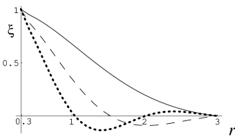
Figure 6.5: Graphic representation of the first three fluctuation modes for $r_{*}=0.3$, $\Lambda=3$ and $l=0$. The three curves have been normalized to have $\xi(r_{*})=1$.

We have performed the numerical integration of the equation of motion of $\xi(r)$ subject to the boundary condition (6.6.14) by means of the shooting technique. For a generic value of the mass $M$ the solution diverges at $r=r_{*}$. Only for some discrete set of masses the fluctuations are regular in the IR. In figure 6.5, we show the first three modes obtained by this procedure for $r_{*}=0.3$ and $\Lambda=3$. From this figure, we notice that the number of zeroes of $\xi(r)$ grows with the mass. In general one observes that the $n^{th}$ mode has $n-1$ nodes in the region $r_{*}<r<\Lambda$, in agreement with the general expectation for this type of boundary value problems. Moreover, for $l=0$, the mass $M$ grows linearly with the number of nodes (see below).

At this point it is interesting to pause a while and discuss the suitability of our election of $r$ as worldvolume coordinate. Although this coordinate is certainly very useful to extract the asymptotic behavior of the fluctuations (specially in the UV), we should keep in mind that we are only describing one half of the brane, i.e. the one corresponding to one of the two hemispheres of the two-sphere. On the other hand, the election of the angle as excited scalar has some subtleties which we now discuss. Actually, to describe the displacement of the brane probe with respect to its unperturbed configuration it is physically more sensible to use the coordinate $y$, defined in eq. (6.4.20). Accordingly, let us define the function $y(r,x,\varphi)$ as

$$y(r,x,\varphi)\,=\,r\sin\theta(r,x,\varphi)\,\,.$$ (6.6.15)

Let us put in this equation $\theta(r,x,\varphi)=\theta_{0}(r)\,+\,\chi(r,x,\varphi)$. At the linear order in $\chi$ we are working, $y$ can be written as

$$y(r,x,\varphi)\,=\,y_{0}(r)\,+\,r\cos\theta_{0}(r)\,\chi(r,x,\varphi)\,\,,$$ (6.6.16)

where $y_{0}(r)\equiv r\sin\theta_{0}(r)$ corresponds to the unperturbed brane. Notice, first of all, that for those modes in which $\chi(r_{*},x,\varphi)$ is finite, the fluctuation term in $y(r_{*},x,\varphi)$ vanishes since $\cos\theta_{0}(r)\rightarrow 0$ when $r\rightarrow r_{*}$. Then

$$y(r_{*},x,\varphi)\,=\,y_{0}(r_{*})\,=\,r_{*}\,\,\,\,{\rm if}\,\,\,\chi(r_{*},x,\varphi)\,\,\,\,{\rm is\,\,\,finite}\,\,.$$ (6.6.17)

Thus, by considering those modes $\chi$ that are regular at $r=r_{*}$ we are effectively restricting ourselves to the modes which have a node in the $y$ coordinate at $r=r_{*}$. If, on the contrary $\chi$ diverges for $r\approx r_{*}$, we know from eq. (6.6.10) that it behaves as $\chi\,\approx\,1/\sqrt{r-r_{*}}$. But we also know that $\cos\theta_{0}(r)\rightarrow 0$ when $r\rightarrow r_{*}$ and, in fact, the second term on the right-hand side of eq. (6.6.16) remains undetermined. The precise form in which $\cos\theta_{0}(r_{*})$ vanishes can be read from eq. (6.8.12), namely $\cos\theta_{0}(r)\,\approx\,\sqrt{r-r_{*}}$ for $r\approx r_{*}$. Therefore, even if $\chi$ diverges at $r=r_{*}$, we could have, in the linearized approximation we are adopting, a finite value for $y(r_{*},x,\varphi)$. Thus, modes with $\chi(r_{*},x,\varphi)\rightarrow\infty$ should not be discarded. Actually, $y(r_{*},x,\varphi)-y_{0}(r_{*})$, although finite, is undetermined in eq. (6.6.16) for these modes and, in order to obtain its allowed values we should impose a boundary condition at the other half of the brane. As previously mentioned, this cannot be done when $r$ is taken as worldvolume coordinate. Therefore, it is convenient to come back to the formalism of sects. 6.2-6.5, in which $\theta$ had been chosen as one of the worldvolume coordinates. In this approach, the unperturbed brane configuration is described by a function $r_{0}(\theta)$, given by:

$$\sinh r_{0}(\theta)\,=\,{\sinh r_{*}\over\sin\theta}\,\,,$$ (6.6.18)

and the brane embedding is characterized by a function $r=r(\theta,x,\varphi)$, which we expand around $r_{0}(\theta)$ as follows:

$$r(\theta,x,\varphi)\,=\,r_{0}(\theta)\,+\,\rho(\theta,x,\varphi)\,\,.$$ (6.6.19)

Plugging this expansion into the DBI lagrangian of eq. (6.4.24) and keeping up to second order terms in $\rho$, one gets the following lagrangian density:

$${\cal L} = -{1\over 2}\,{e^{2\phi}\sin\theta\,r_{0}\over r_{0}+\cot^{2}\theta\tanh r_{0}}\Bigg{[}\coth r_{0}\,\big{(}\partial_{\theta}\rho\big{)}^{2}+{2\cot\theta\over\sinh r_{0}\cosh r_{0}}\,\,\rho\partial_{\theta}\rho+{\cot^{2}\theta\over\sinh r_{0}\cosh^{3}r_{0}}\,\rho^{2}\,\Bigg{]}-$$ (6.6.20)

$$\,\,-\,\,{e^{2\phi}\sin\theta\,\,r_{0}\over 2}\,\Bigg{[}\,\big{(}\partial_{x}\,\rho\,\big{)}^{2}\,+\,{1\over\cos^{2}\theta\,\big{(}1+r_{0}\coth r_{0}\tan^{2}\theta\,\big{)}}\,\,\big{(}\partial_{\varphi}\,\rho\,\big{)}^{2}\,\Bigg{]}\,\,.$$

Similarly to what we have done with the lagrangian (6.6.5), we will look for solutions of the equations of motion of ${\cal L}$ which have the form:

$$\rho(\theta,x,\varphi)\,=\,e^{ikx}\,e^{il\varphi}\,\,\zeta(\theta)\,\,,$$ (6.6.21)

where $l$ is an integer and $k^{2}=-M^{2}$. As before, in order to get a discrete spectrum one must impose some boundary conditions. In the present approach we should cutoff the regions close to the two poles of the two-sphere. Accordingly, let us define the following angle:

$$\sin\theta_{\Lambda}\equiv{\sinh r_{*}\over\sinh\Lambda}\,\,,\,\,\,\,\,\,\,\,\,\,\,\,\,\,\,\theta_{\Lambda}\in(0,{\pi\over 2})\,\,,$$ (6.6.22)

where, as indicated, we are taking $\theta_{\Lambda}$ in the range $0<\theta_{\Lambda}<\pi/2$. Notice that $\theta_{\Lambda}\rightarrow 0$ if $\Lambda\rightarrow\infty$ as it should. Clearly $\theta_{\Lambda}$ and $\pi-\theta_{\Lambda}$ are the two angles that correspond to the radial scale $\Lambda$. Therefore, we impose the following boundary conditions to our fluctuation:

$$\zeta(\theta_{\Lambda})\,=\,\zeta(\pi-\theta_{\Lambda})\,=\,0\,\,.$$ (6.6.23)

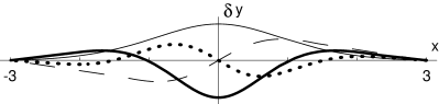
Figure 6.6: Plot of $\delta y\equiv\zeta\sin\theta$ versus $x=r\cos\theta$ for the first four modes for $r_{*}=0.3$, $\Lambda=3$ and $l=0$. The dashed and dotted curves pass through the origin and correspond to the first two modes of figure 6.5.

The equations of motion derived from (6.6.20), subjected to the boundary conditions (6.6.23) can be integrated numerically by means of the shooting technique. One first enforces the condition at $\theta=\theta_{\Lambda}$ and then varies the mass $M$ until $\zeta(\pi-\theta_{\Lambda})$ vanishes. This only happens for a discrete set of values of the mass $M$. For a given value of $l$, let us order the solutions in increasing value of the mass. In general one notices that the $n^{th}$ mode has $n-1$ nodes in the interval $\theta_{\Lambda}<\theta<\pi-\theta_{\Lambda}$ and for $n$ even (odd) the function $\zeta(\theta)$ is odd (even) under $\theta\rightarrow\pi-\theta$. In figure 6.6, we have plotted the first four modes corresponding to $r_{*}=0.3$, $\Lambda=3$ and $l=0$. The modes odd under $\theta\rightarrow\pi-\theta$ vanish at $\theta=\pi/2$ and their masses and shapes match those found with the lagrangian (6.6.5) and the boundary condition (6.6.14). On the contrary, the modes with an even number of nodes in $\theta_{\Lambda}<\theta<\pi-\theta_{\Lambda}$ are the ones we were missing in the formulation in which $r$ is taken as worldvolume coordinate.

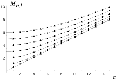
Figure 6.7: Mass spectrum for $r_{*}=0.3$ and $\Lambda=3$ for $l=0,\cdots,6$. The solid lines correspond to the right-hand side of eq. (6.6.24). The triangles (squares) are the masses of the modes $\zeta(\theta)$ which are even (odd) under $\theta\rightarrow\pi-\theta$.

Let $M_{n,l}(r_{*},\Lambda)$ be the mass corresponding to the $n^{th}$ mode for a given value $l$ and the mass scales $r_{*}$ and $\Lambda$. Our numerical results are compatible with an expression of $M_{n,l}(r_{*},\Lambda)$ of the form:

$$M_{n,l}(r_{*},\Lambda)\,=\,\sqrt{m^{2}(r_{*},\Lambda)\,\,n^{2}+l^{2}}$$ (6.6.24)

To illustrate this fact we have plotted in figure 6.7 the values of $M_{n,l}(r_{*},\Lambda)$ for $r_{*}=0.3$ and $\Lambda=3$, together with the curves corresponding to the right-hand side of (6.6.24).

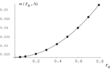
Figure 6.8: Dependence of $m(r_{*},\Lambda)$ on $r_{*}$ for $\Lambda=3$. The solid line is a fit to the quadratic function (6.6.25).

We have also studied the dependence of the coefficient $m(r_{*},\Lambda)$ on the two scales $(r_{*},\Lambda)$. Recall that $r_{*}$ is the minimal separation of the brane probe from the origin and, thus, can be naturally identified with the mass of the quarks. We obtained that $m(r_{*},\Lambda)$ can be represented by an expression of the type:

$$m(r_{*},\Lambda)\,=\,{\pi\over 2\Lambda}\,+\,b(\Lambda)\,r^{2}_{*}\,\,.$$ (6.6.25)

The coefficients on the right-hand side of eq. (6.6.25) have been obtained by a fit of $m(r_{*},\Lambda)$ to a quadratic expression in $r_{*}$. An example of this fit is presented in figure 6.8. The first term in eq. (6.6.25) is a universal term (independent of $r_{*}$) which can be regarded as a finite size effect induced by our regularization procedure. We also have determined the dependence of the coefficient $b$ on $\Lambda$ and it turns out that one can fit $b(\Lambda)$ to the expression $b(\Lambda)=0.23\,\Lambda^{-2}\,+\,0.53\,\Lambda^{-3}$ .

We have obtained a very regular mass spectrum of particles, classified by two quantum numbers $n,l$ (see eqs. (6.6.24) and (6.6.25)). We can offer an interpretation of these formulas. Indeed, recall that the two-submanifold on which we are wrapping the brane is topologically like a cylinder, with the compact direction parametrized by the angle $\varphi$. The quantum number $l$ is precisely the eigenvalue of the operator $-i\partial_{\varphi}$, which generates the shifts of $\varphi$ and, indeed, the dependence on $l$ of the mass displayed in eq. (6.6.24) is the typical one for a Kaluza-Klein reduction along a compact coordinate. Therefore, we should interpret the mesons with $l\not=0$ as composed by Kaluza-Klein modes. Moreover, the term in (6.6.25) proportional to $r_{*}^{2}$ can be understood as the contribution coming from the mass of the constituent quarks, while the term $\frac{\pi}{2\Lambda}$ can be interpreted as a contribution coming from the ‘finite size‘ of the meson. Indeed, it looks like a Casimir energy and it is originated in the presence of the cut-off $\Lambda$.

It is perhaps convenient to emphasize again that the cut-off procedure implemented here is a very natural procedure for this type of computations in this supergravity dual. In fact, given that the mesons are an IR effect in SQCD, we expect the contributions of high energy effects to be irrelevant or negligible in the physical properties of the meson itself. This is indeed what we are doing when cutting off the integration range. We are just taking into account the ‘non-abelian‘ part of the probes, while neglecting the ‘abelian‘ part or, equivalently, discarding high energy contributions.

6.6.2 Vector mesons

Let us now excite a gauge field that is living in the worldvolume of the brane. The linearized equations of motion are:

$$\partial_{m}\,\Big{[}\,e^{-\phi}\,\sqrt{-g_{st}}\,{\cal F}^{nm}\,\Big{]}\,=\,0\,\,,$$ (6.6.26)

where $g_{st}$ is the determinant of the induced metric in the string frame and ${\cal F}^{nm}$ is the field strength of the worldvolume gauge field ${\cal A}_{m}$, i.e. ${\cal F}_{nm}=\partial_{n}{\cal A}_{m}-\partial_{m}{\cal A}_{n}$. Let us assume that the only non-vanishing components of the gauge field ${\cal A}$ are those along the unwrapped directions $x^{\mu}$ of the worldvolume of the brane. In what follows we are going to use $\theta$ as worldvolume coordinate. Let us put

$${\cal A}_{\mu}(\theta,x,\varphi)\,=\,\epsilon_{\mu}\,\varsigma(\theta)\,\,e^{ikx}\,\,e^{il\varphi}\,\,,$$ (6.6.27)

where $\epsilon_{\mu}$ is a constant polarization four-vector and $l$ must be an integer. It follows from the equations of motion (6.6.26) that $\epsilon_{\mu}$ must be transverse, i.e.:

$$k^{\mu}\,\epsilon_{\mu}\,=\,0\,\,,$$ (6.6.28)

and that $\varsigma(\theta)$ must satisfy the following second-order differential equation:

$$\partial_{\theta}\,\Big{[}\,{\sin\theta\over\tanh r_{0}}\,\partial_{\theta}\,\varsigma\,\Big{]}\,+\,{\tanh r_{0}\over\sin\theta}\,\,\Bigg{[}\,M^{2}\,\,\bigg{(}\cos^{2}\theta\,+\,r_{0}\,\coth r_{0}\,\sin^{2}\theta\bigg{)}\,-\,l^{2}\,\Bigg{]}\varsigma\,=\,0\,\,,$$ (6.6.29)

where, as in eq. (6.6.7), $k^{2}=-M^{2}$. We have solved numerically this equation by means of the shooting technique with the boundary conditions

$$\varsigma(\theta_{\Lambda})\,=\,\varsigma(\pi-\theta_{\Lambda})\,=\,0\,\,.$$ (6.6.30)

Surprisingly, the set of possible values of $M$ is given by the same expression as in the scalar meson case, i.e. eq. (6.6.24), with a coefficient function $m(r_{*},\Lambda)$ which is, within the accuracy of our approximate calculation, equal numerically to that of the scalar mesons. This is quite remarkable since the differential equations we are solving in both cases are quite different (the equation satisfied by $\zeta(\theta)$, which arises from the lagrangian (6.6.20), is much more complicated than eq. (6.6.29)). Thus, to summarize, we predict a degeneracy between the scalar and vector mesons in the corresponding ${\cal N}=1$ SYM theory.

6.6.3 Gauge theory interpretation

Let us comment on some gauge theory aspects that can be read from the results of this chapter. For this purpose, we shall concentrate on the main solutions that have been used, namely, the abelian solution with unit winding ($n=1$) in eq. (6.4.22) and its non-abelian extension of eq. (6.5.15).

First of all, let us analyze the R-symmetry of the gauge theory from the probe viewpoint. It is clear that the abelian solution (6.4.22) is invariant under shifts of $\tilde{\psi}$ by a constant since the value of this angle is an arbitrary constant in this solution. This symmetry has been identified as the geometric dual of the R-symmetry [37, 110, 48]. Actually, this is not a $U(1)$ invariance of the background because [37, 110, 48] of the presence of the RR form that selects, by consistency, only some particular values of the angle $\tilde{\psi}$, i.e. $\tilde{\psi}=\frac{2\pi n}{N}$ with $1\leq n\leq 2N$. So, the abelian probes can see a ${\rm Z}\kern-3.8pt{\rm Z}\kern 2.0pt_{2N}$ symmetry. In contrast, when we consider the non-abelian probe, the solution (6.5.15) selects two particular values of the angle $\tilde{\psi}$, thus breaking ${\rm Z}\kern-3.8pt{\rm Z}\kern 2.0pt_{2N}$ down to ${\rm Z}\kern-3.8pt{\rm Z}\kern 2.0pt_{2}$. Notice that the $U(1)\rightarrow{\rm Z}\kern-3.8pt{\rm Z}\kern 2.0pt_{2N}$ breaking is an UV effect (it takes place already in the abelian background) while the ${\rm Z}\kern-3.8pt{\rm Z}\kern 2.0pt_{2N}\rightarrow{\rm Z}\kern-3.8pt{\rm Z}\kern 2.0pt_{2}$ breaking is an IR effect which appears only when one considers the full non-abelian regular background. This same breaking pattern was observed in the case of SQCD with massive flavors. Indeed, as showed in [109], the theory with massive flavors has a non-anomalous discrete ${\rm Z}\kern-3.8pt{\rm Z}\kern 2.0pt_{2N}$ R-symmetry, given by (component fields are used, $\lambda$ is the gluino and $\Phi$ and $\bar{\Phi}$ are the squarks):

$$\lambda\rightarrow e^{-i\pi n/N}\lambda\,\,,~{}\,\,\,\,\,\,\,\,\Phi\rightarrow e^{-i\pi n/N}\Phi\,\,,\,\,\,\,\,\,\,\,\bar{\Phi}\rightarrow e^{-i\pi n/N}\bar{\Phi}\,\,,$$ (6.6.31)

with $n=1,...2N$ .

As shown in [109], this ${\rm Z}\kern-3.8pt{\rm Z}\kern 2.0pt_{2N}$ symmetry is broken down to ${\rm Z}\kern-3.8pt{\rm Z}\kern 2.0pt_{2}$ by the formation of a squark condensate. Indeed, one can see that $<\Phi\bar{\Phi}>$ transforms as $<\Phi\bar{\Phi}>\rightarrow e^{-2i\pi n/N}<\Phi\bar{\Phi}>$ leaving us with a ${\rm Z}\kern-3.8pt{\rm Z}\kern 2.0pt_{2}$. Besides, the squark condensate is consistent with supersymmetry, because the $F$-term equation of motion $<\Phi\bar{\Phi}>-m=0$ is satisfied. Notice that this preservation of symmetry when $m\not=0$ is in agreement with the kappa symmetry of our brane probes.

Apart from all this, there is a vectorial $U(1)$ symmetry that remains unbroken in our brane probe analysis and that we have associated with the invariance under translations in $\tilde{\varphi}$. On the field theory side, this symmetry can be identified with a phase change of the full chiral/antichiral multiplet $\Phi\rightarrow e^{i\alpha}\Phi,\,\,\bar{\Phi}\rightarrow e^{-i\alpha}\bar{\Phi}$, which is nothing but the $U(1)_{B}$ baryonic number symmetry of the theory. The two possible assignations $\pm 1$ of the baryonic charge are in correspondence with the two possible identifications of the $S^{1}$ described by $\tilde{\varphi}$ with the $S^{1}$ parametrized by $\varphi$. The spectrum we have found is independent of this identification.

We would like also to comment briefly on the possibility of taking the parameter $r_{*}=0$. Given that this parameter can be associated with the mass of the quark (since it is the characteristic distance between the probe brane and the background), one would like to study the case in which this parameter is taken to be zero. Nevertheless, the approach implemented here seems to break down for this particular value of the parameter. Indeed, taking $r_{*}=0$ will imply that $\theta_{0}=0$, so, a fluctuation of it can lead to negative values of $\theta$ taking us out of the range of this coordinate. The fact that our approach apparently does not work for the case of massless quarks seems to be in agreement with the fact that SQCD with massless flavors, has some special properties like spontaneous breaking of supersymmetry, the existence of a runaway potential (Affleck-Dine-Seiberg potential) and the non-existence of a well-defined vacuum state. Notice that, when $r_{*}\not=0$, our approach, by construction, deals with massive quarks that preserve supersymmetry, since our probes were constructed by that requirement.

6.7 Discussion

In this chapter, a search for surfaces where a D5-brane can be placed in the Maldacena-Núñez background without spoiling supersymmetry has been performed.

Solutions where the probes are at a fixed distance from the ”background branes” are shown to break supersymmetry. This phenomenon is in agreement with the non-existence of moduli space of ${\cal N}=1$ SYM. On the other hand, allowing the distance to the brane probe to vary, a wide variety of kappa symmetric solutions was found and a rich mathematical structure was pointed out. Typically, these probes extend to infinity. On the spirit of AdS/CFT correspondence, when the gravity setup is changed at infinity, some new ingredient is introduced in the associated gauge theory. In our case, we interpret the configurations found (at least some of them) as the introduction of flavor in the dual ${\cal N}=1$ SYM.

First, configurations in the abelian background (the large $r$ regime of the full background) have been studied. These abelian solutions are shown to have a very interesting analytic structure (harmonic functions and Cauchy-Riemann equations show up) allowing interesting explicit solutions. In extending these studies to the full background, we found several classes of non-abelian solitons. It might be possible that these solutions show themselves useful when studying other aspects of the model not addressed in this work.

Then, in section (6.6), the kappa symmetric solutions which are argued to introduce fundamental matter in the dual to SYM theory (those we called unit-winding) have been explored in detail. The surfaces where the flavor branes are placed are the equivalent of the non-compact holomorphic 2-cycles considered in ref. [38] to add chiral superfields in a similar scenario.

Given that the brane probes do not backreact on the background, these flavors are introduced in the so-called quenched approximation. Nevertheless, many qualitative features and quantitative predictions for the strong coupling regime of ${\cal N}=1$ SQCD can be addressed. Among them, the qualitative difference between the massless and massive flavors is clear in this picture. Indeed, by construction, our approach deals with the massive-flavor case, so, the problems or peculiarities of the massless case can be seen in this approach under a different geometrical perspective.

Other characteristic feature of SQCD with few flavors is the breaking pattern of R-symmetry. The ${\rm Z}\kern-3.8pt{\rm Z}\kern 2.0pt_{2N}\rightarrow{\rm Z}\kern-3.8pt{\rm Z}\kern 2.0pt_{2}$ breaking is geometrically very clear from the brane probe perspective. Also, the preserved vectorial symmetry $U(1)_{B}$ is geometrically realized, as explained in the previous section, by arbitrary changes in the coordinate $\tilde{\varphi}$.

A mass spectrum for the low energy excitations (mesons) of massive SQCD was found and this may be a very interesting and quantitative prediction of this approach. In fact, a nice formula for the masses is derived that exhibits a BPS-like behavior with the level ($n$) and with the Kaluza-Klein quantum number ($l$) of the meson (6.6.24), (6.6.25). Basically, our formula gives the meson masses in terms of the mass of the fundamentals and the Casimir energy due to finite size of the meson, and shows explicitly the contamination of the meson spectrum due to the Kaluza-Klein modes. It would be very interesting if lattice calculations could validate or invalidate the formula found here.

Our results are in perfect agreement with two general assertions about vector-like gauge theories proved by Vafa and Witten [111]: massive quarks cannot constitute massless mesons and a vectorial symmetry cannot be spontaneously broken.

It would be really interesting to find a backreacted gravity solution in order to go beyond the quenched approximation of the gauge theory. Among other aspects, the Affleck-Dine-Seiberg potential, the corrections to the $\beta$-function due to flavors or Seiberg dualities might be found. The techniques developed will hopefully be useful to perform similar analysis in different gravity setups.

6.8 Appendix: asymptotic behavior of the fluctuations

This appendix is devoted to the determination of the asymptotic form of the fluctuations around the kappa-symmetric static configurations of the D5-brane probe. In subsection 6.8.1 we will consider the large and small $r$ behavior of the solutions of the equation of motion corresponding to the lagrangian (6.6.5), which describes the small oscillations around the unit-winding embedding (6.6.2). In section 6.8.2 we will study the asymptotic form of the fluctuations of the $n$-winding embedding in the abelian background. Following our general arguments, the UV behavior of the abelian and non-abelian fluctuations must be the same and, thus, from this analysis we can get an idea of the nature of the small oscillations around the general non-abelian $n$-winding configurations (whose analytical form we have not determined) for large values of the radial coordinate.

6.8.1 Non-abelian unit-winding embedding

For large $r$ the lagrangian (6.6.5) takes the form:

$${\cal L}\,=\,-{1\over 2}\,e^{2\phi}\,\big{[}\,r\,(\partial_{r}\chi)^{2}\,+\,2r\,\chi\,\partial_{r}\chi\,+\,r\chi^{2}\,+\,r\,(\partial_{x}\chi)^{2}\,+\,r\,(\partial_{\varphi}\chi)^{2}\,\big{]}\,\,,$$ (6.8.1)

where we have not expanded the dilaton and we have eliminated the exponentially suppressed terms. Using the asymptotic value of $\partial_{r}\phi$:

$$\partial_{r}\phi\,\approx\,1\,-{1\over 4r-1}\,\,,$$ (6.8.2)

we obtain the following equation for $\xi$:

$$\partial^{2}_{r}\,\xi\,+\,{8r^{2}-1\over 4r^{2}-r}\,\partial_{r}\,\,\xi\,+\,\Bigg{(}M^{2}-l^{2}+1\,+\,{2r-1\over 4r^{2}-r}\Bigg{)}\,\,\xi\,=\,0\,\,.$$ (6.8.3)

To study the UV behavior of the solutions of this differential equation, it is interesting to rewrite it with the different coefficient functions expanded in powers of $1/r$ as:

$$\partial^{2}_{r}\,\xi\,+\,\big{(}\,a_{0}+{a_{1}\over r}+{a_{2}\over r^{2}}\,+\,\cdots\big{)}\,\partial_{r}\,\xi\,+\,\big{(}\,b_{0}+{b_{1}\over r}+{b_{2}\over r^{2}}\,+\,\cdots\big{)}\,\xi\,=\,0\,\,,$$ (6.8.4)

where:

$$a_{0}\,=\,2\,,\,\,\,\,\,\,\,\,b_{0}\,=\,M^{2}-l^{2}+1\,,\,\,\,\,\,\,\,\,\,\,\,\,\,\,\,\,\,\,\,\,a_{1}\,=\,b_{1}\,=\,{1\over 2}\,,\,\,\,\,\,\,\,\,\,\,\,\,\,\,\,a_{2}\,=\,b_{2}\,=\,-{1\over 8}\,,\cdots\\ \\$$

We want to solve eq. (6.8.4) by means of an asymptotic Frobenius expansion of the type $\xi=r^{\rho}\,(c_{0}+c_{1}/r+\cdots)$ for some exponent $\rho$. By substituting this expansion on the right-hand side of eq. (6.8.4) and comparing the terms with the different powers of $r$, we notice that there is only one term with $r^{\rho}$, namely $b_{0}c_{0}r^{\rho}$, which cannot be canceled. In order to get rid of this term, let us define a new function $w$ as:

$$\xi\,=\,e^{\alpha r}\,w\,\,,$$ (6.8.5)

with $\alpha$ being a number to be determined. The equation satisfied by $w$ is the same as that of $\xi$ with the changes:

$$a_{0}\rightarrow a_{0}+2\alpha\,,\,\,\,\,\,\,\,\,\,\,\,\,\,\,\,\,b_{0}\rightarrow\alpha^{2}+\alpha a_{0}+b_{0}\,\,,$$

$$a_{i}\rightarrow a_{i}\,\,,\,\,\,\,\,\,\,\,\,\,\,\,\,\,\,\,\,\,\,\,\,\,\,\,\,\,\,b_{i}\rightarrow b_{i}+\alpha a_{i}\,\,,\,\,\,\,\,\,\,\,(i=1,2,\cdots)\,\,.$$ (6.8.6)

It is clear that we must impose the condition:

$$\alpha^{2}+\alpha a_{0}+b_{0}\,=\,0\,\,,$$ (6.8.7)

which determines the values of $\alpha$. Writing now $w=r^{\rho}\,(c_{0}+c_{1}/r+\cdots)$ and looking at the highest power of $r$ in the equation of $w$ (i.e. $\rho-1$), we immediately obtain the value of $\rho$, namely:

$$\rho=-{\alpha a_{1}+b_{1}\over 2\alpha+a_{0}}\,\,,$$ (6.8.8)

and, clearly, as $r\rightarrow\infty$ the asymptotic behavior of $\xi(r)$ is:

$$\xi(r)\approx e^{\alpha r}\,r^{\rho}\,(\,1\,+\,o({1\over r})\,)\,\,.$$ (6.8.9)

In our case, it is easy to verify that the values of $\alpha$ and $\rho$ are:

$$\alpha=-1\pm i\sqrt{M^{2}-l^{2}}\,\,,\,\,\,\,\,\,\,\,\,\,\,\,\rho=-{1\over 4}\,\,.$$ (6.8.10)

Then, it is clear that we have two independent behaviors for the real function $\xi(r)$, namely:

$$\xi(r)\sim{e^{-r}\over r^{{1\over 4}}}\cos\Big{(}\,\sqrt{M^{2}-l^{2}}\,\,r\,\Big{)}\,,\,\,\,\,\,\,{e^{-r}\over r^{{1\over 4}}}\sin\Big{(}\,\sqrt{M^{2}-l^{2}}\,\,r\,\Big{)}\,\,.$$ (6.8.11)

Notice that all solutions decrease exponentially when $r\rightarrow\infty$.

Let us now turn to the analysis of the fluctuations for small values of the radial coordinate. Recall that $r_{*}\leq r\leq\infty$. Near $r_{*}$, one can expand $\sin\theta_{0}$ and $\cos\theta_{0}$ as follows:

$$\sin\theta_{0} \approx 1\,-\,\coth r_{*}\,(r-r_{*})\,+\,{1\over 2}\,{1+\cosh^{2}r_{*}\over\sinh^{2}r_{*}}\,(r-r_{*})^{2}\,+\,\cdots\,\,,$$

$$\cos\theta_{0} \approx \sqrt{2\coth r_{*}(r-r_{*})}\,\bigg{[}\,1\,-{\coth r_{*}\over 2}\,(1+{1\over 2\cosh^{2}r_{*}})\,(r-r_{*})\,+\,\cdots\bigg{]}\,\,.$$ (6.8.12)

Using these expressions it is straightforward to show that the lagrangian density of the quadratic fluctuations is given by:

$${\cal L}\,=\,-{1\over 2}\,e^{2\phi_{*}}\,\,\big{[}\,A(r)\,(\,\partial_{r}\chi)^{2}\,+\,B(r)2\chi\partial_{r}\chi\,+\,C(r)\,\chi^{2}\,+\,D(r)\,(\,\partial_{x}\chi)^{2}\,+\,E(r)\,(\,\partial_{\varphi}\chi)^{2}\,\,\big{]}\,\,,$$ (6.8.13)

where $\phi_{*}=\phi(r_{*})$ and the functions $A,B,C,D$ and $E$ are of the form:

$$A(r) = \big{[}\,8\tanh r_{*}\,(r-r_{*})^{3}\,\big{]}^{{1\over 2}}\,\,\big{(}\,1\,+\,{\cal A}(r)\,\big{)}\,\,,$$

$$B(r) = {\sqrt{2(r-r_{*})}\over\sqrt{\coth r_{*}}}\,\,\big{(}\,1\,+\,{\cal B}(r)\,\big{)}\,\,,$$

$$C(r) = {1\over\sqrt{2\coth r_{*}\,(r-r_{*})}}\,\,\big{(}\,1\,+\,{\cal C}(r)\,\big{)}\,\,,$$

$$D(r) = {r_{*}\over\sqrt{\coth r_{*}}}\,\sqrt{2(r-r_{*})}\,\,\big{(}\,1\,+\,{\cal D}(r)\,\big{)}\,\,,$$

$$E(r) = \big{[}\,\tanh r_{*}\,\big{]}^{{3\over 2}}\,\,\sqrt{2(r-r_{*})}\,\,\big{(}\,1\,+\,{\cal E}(r)\,\big{)}\,\,.$$ (6.8.14)

The functions ${\cal A},{\cal B},{\cal C},{\cal D},{\cal E}$, satisfy:

$${\cal A}(r),{\cal B}(r),{\cal C}(r),{\cal D}(r)\,{\cal E}(r)\,\,\sim\,\,o(r-r_{*})\,\,.$$ (6.8.15)

Notice that, remarkably, after integrating by parts the $\chi\partial_{r}\chi$ term in the lagrangian, the singular term of $C(r)$ cancels against the leading term of $B(r)$. The equation of motion for $\xi$ near $r_{*}$ is:

$$\partial^{2}_{r}\xi\,+\,{A^{\prime}(r)\over A(r)}\,\,\partial_{r}\xi\,+\,{B^{\prime}(r)-C(r)+M^{2}D(r)-l^{2}E(r)\over A(r)}\,\,\xi\,=\,0\,\,.$$ (6.8.16)

In order to solve this equation in a power series expansion in $r-r_{*}$, it is important to understand the singularities of the different coefficients near $r_{*}$. It is immediate that:

$${A^{\prime}(r)\over A(r)}\,=\,{3\over 2}\,\,{1\over r-r_{*}}\,+\,{{\cal A}^{\prime}(r)\over 1+{\cal A}(r)}\,=\,{3\over 2}\,\,{1\over r-r_{*}}\,+\,{\rm regular}\,\,.$$ (6.8.17)

Similarly, the coefficient of $\xi$ has a simple pole near $r_{*}$:

$${B^{\prime}(r)-C(r)+M^{2}D(r)-l^{2}E(r)\over A(r)}\,=\,{3{\cal B}\,^{\prime}(r_{*})-{\cal C}\,^{\prime}(r_{*})+2M^{2}r_{*}-2l^{2}\tanh r_{*}\over 4}\,{1\over r-r_{*}}\,+\,{\rm regular}\,\,.$$

It follows that the point $r=r_{*}$ is a singular regular point. The corresponding Frobenius expansion reads:

$$\xi(r)\,=\,(r-r_{*})^{\lambda}\,\sum_{n=0}^{\infty}\,c_{n}\,(r-r_{*})^{n}\,\,,$$ (6.8.19)

where $\lambda$ satisfies the indicial equation, which can be obtained by plugging the expansion in the equation and looking at the term with lowest power of $r-r_{*}$ (i.e. $\lambda-2$). In our case, $\lambda$ must be a root of the quadratic equation:

$$\lambda(\lambda-1)+{3\over 2}\,\lambda\,=\,0\,\,,$$ (6.8.20)

i.e.:

$$\lambda=0,-{1\over 2}\,\,.$$ (6.8.21)

This means that there are two independent solutions of the differential equation which can be represented by a Frobenius series around $r=r_{*}$, one of then is regular as $r\rightarrow r_{*}$ (the one corresponding to $\lambda=0$), whereas the other diverges as $(r-r_{*})^{-{1\over 2}}$.

6.8.2 $n$-Winding embeddings in the abelian background

Let us consider the abelian background and an embedding with winding number $n$, for which $\partial_{\varphi}\tilde{\varphi}=n$, $\sin\theta\partial_{\theta}\tilde{\theta}\,=\,n\sin\tilde{\theta}$ and $\psi=\psi_{0}={\rm constant}$. Let us define:

$$V \equiv {n\over 2}{\cos\tilde{\theta}\over\sin\theta}\,+\,{1\over 2}\cot\theta\,=\,{n\over 2\sin\theta}\,\,{(1+\cos\theta)^{n}\,-\,(1-\cos\theta)^{n}\over(1+\cos\theta)^{n}\,+\,(1-\cos\theta)^{n}}\,+\,{1\over 2}\cot\theta\,\,,$$

$$W \equiv {n\over 2}{\sin\tilde{\theta}\over\sin\theta}\,=\,{n(\sin\theta)^{(n-1)}\over(1+\cos\theta)^{n}\,+\,(1-\cos\theta)^{n}}\,\,.$$ (6.8.22)

Choosing $r$ as worldvolume coordinate and considering embeddings in which $\theta$ depends on both $r$ and on the unwrapped coordinates $x$, we obtain the following lagrangian:

$${\cal L}=-e^{2\phi}\,\sin\theta \Bigg{[} \sqrt{\big{(}\,e^{2h}\,+\,V^{2}\,+\,W^{2}\,\big{)}\,\big{(}\,1\,+\,(e^{2h}\,+\,W^{2})((\partial_{r}\theta)^{2}\,+\,(\partial_{x}\theta)^{2})\big{)}}\,+$$ (6.8.25)

$$+\,(e^{2h}\,+\,W^{2})\partial_{r}\theta\,-\,V\,\Bigg{]}\,\,.$$

We shall expand this lagrangian around a configuration $\theta_{0}(r)$ such that:

$$e^{2(r-r_{*})}\,=\,{1\over 2}\,{(1+\cos\theta_{0}(r))^{n}\,+\,(1-\cos\theta_{0}(r))^{n}\over(\sin\theta_{0}(r))^{n+1}}\,\,.$$ (6.8.26)

Notice that $\theta_{0}(r)$ remains unchanged under the transformation $n\rightarrow-n$. Thus, without loss of generality we shall restrict ourselves from now on to the case $n\geq 0$. Let us now define:

$$V_{0}(r)\equiv V|_{\theta(r)=\theta_{0}(r)}\,\,,\,\,\,\,\,\,\,\,\,\,\,\,\,\,\,\,W_{0}(r)\equiv W|_{\theta(r)=\theta_{0}(r)}\,\,,\,\,\,\,\,\,\,\,\,\,\,\,\,\,\,\,V_{0\theta}(r)\equiv{\partial V\over\partial\theta}\Big{|}_{\theta(r)=\theta_{0}(r)}\,\,.$$ (6.8.27)

Using:

$$\partial_{r}\theta_{0}\,=\,-{1\over V_{0}}\,\,,$$ (6.8.28)

we obtain the following quadratic lagrangian:

$${\cal L}\,=\,-{e^{2\phi}\over 2}\,\sin\theta_{0}\,(e^{2h}\,+\,W_{0}^{2}\,)\, \Bigg{[} {1\over e^{2h}\,+\,V_{0}^{2}\,+\,W_{0}^{2}}\,\Big{(}\,V_{0}^{3}\,(\partial_{r}\chi)^{2}\,-\,2V_{0}\,V_{0\theta}\,\chi\partial_{r}\chi\,+$$ (6.8.29)

$$+\,{V_{0\theta}^{2}\over V_{0}}\,\chi^{2}\,\Big{)}\,+\,V_{0}\,(\partial_{x}\chi)^{2}\,\Bigg{]}\,\,.$$

Keeping the leading terms for large $r$, the lagrangian becomes:

$${\cal L}\,=\,-{r\over 2}e^{2\phi}\,\big{[}\,{n+1\over 2}\,(\partial_{r}\chi)^{2}\,+\,2\chi\partial_{r}\chi\,+\,{2\over n+1}\,\chi^{2}\,+\,{n+1\over 2}\,(\partial_{x}\chi)^{2}\,\big{]}\,\,,$$ (6.8.30)

and, if we represent $\chi$ as in eq. (6.6.6) with $l=0$, the equation of motion for $\xi$ becomes:

$$\partial_{r}^{2}\xi\,+\,\big{(}2+{1\over 2r}\big{)}\,\partial_{r}\xi\,+\,\bigg{(}\,M^{2}\,+\,{4n\over(n+1)^{2}}\,+\,{1\over n+1}\,{1\over r}\,\bigg{)}\,\xi\,=\,0\,\,.$$ (6.8.31)

Now we have the following coefficients in eq. (6.8.4):

$$a_{0}\,=\,2\,\,,\,\,\,\,\,\,\,\,\,\,\,\,\,\,\,\,\,\,b_{0}\,=\,M^{2}+{4n\over(n+1)^{2}}\,\,,\,\,\,\,\,\,\,\,\,\,\,\,\,\,\,\,\,\,a_{1}\,=\,{1\over 2}\,\,,\,\,\,\,\,\,\,\,\,\,\,\,\,\,\,\,\,\,b_{1}\,=\,{1\over n+1}\,\,.$$ (6.8.32)

By plugging these values in eq. (6.8.7), we obtain the following result for the coefficient $\alpha$ of the exponential:

$$\alpha\,=\,-1\,\pm\,\sqrt{\Big{(}{n-1\over n+1}\Big{)}^{2}\,-\,M^{2}}\,\,.$$ (6.8.33)

Let us distinguish two cases, depending on the sign inside the square root. Suppose first that $M^{2}\geq\big{(}{n-1\over n+1}\big{)}^{2}$ and define:

$$\tilde{M}^{2}\,=\,M^{2}\,-\,\Big{(}{n-1\over n+1}\Big{)}^{2}\,\,.$$ (6.8.34)

In this case the values of the exponent $\rho$ obtained from (6.8.8) are:

$$\rho\,=\,-{1\over 4}\,\mp{n-1\over 2(n+1)\tilde{M}}\,\,i\,\,.$$ (6.8.35)

It follows that the two real asymptotic solutions are:

$$\xi(r)\sim{e^{-r}\over r^{{1\over 4}}}\,\cos\big{[}\tilde{M}r\,-\,{n-1\over 2(n+1)\tilde{M}}\,\log r\big{]}\,\,,\,\,\,\,\,\,\,\,\,\,\,\,{e^{-r}\over r^{{1\over 4}}}\,\sin\big{[}\tilde{M}r\,-\,{n-1\over 2(n+1)\tilde{M}}\,\log r\big{]}\,\,.$$ (6.8.36)

Both solutions vanish exponentially when $r\rightarrow\infty$.

If $\tilde{M}^{2}<0$, let us define $\bar{M}^{2}=-\tilde{M}^{2}$. In this case $\alpha$ is real, namely $\alpha=-1\pm\bar{M}$. Notice that $\bar{M}<1$ and thus $\alpha<0$. The independent asymptotic solutions are:

$$\xi(r)\sim e^{(\bar{M}-1)r}\,\,r^{-{1\over 4}\,\big{(}1\,-\,{n-1\over(n+1)\bar{M}}\big{)}}\,\,,\,\,\,\,\,\,\,\,\,\,\,\,e^{-(\bar{M}+1)r}\,\,r^{-{1\over 4}\,\big{(}1\,+\,{n-1\over(n+1)\bar{M}}\big{)}}\,\,,$$ (6.8.37)

and both decrease exponentially, without oscillations, when $r\rightarrow\infty$. This non-oscillatory character of the functions in eq. (6.8.36) make them inadequate for the type of boundary conditions we are imposing and, therefore, we shall discard them.

Notice that, for $n=1$, the large $r$ asymptotic solutions (6.8.11) and (6.8.36) coincide. This is of course to be expected since the abelian and non-abelian configurations coincide in the UV. It is also interesting to compare the magnitude of the fluctuation with that of the unperturbed configuration for large $r$. By inspecting eq. (6.8.26) one readily concludes that:

$$\theta_{0}(r)\,\sim\,e^{-{2\over n+1}r}\,\,,\,\,\,\,\,\,\,\,\,(r\rightarrow\infty)\,\,.$$ (6.8.38)

By comparing this behavior with eq. (6.8.36) one finds:

$${\xi(r)\over\theta_{0}(r)}\sim{e^{-{n-1\over n+1}r}\over r^{{1\over 4}}}\,\,,\,\,\,\,\,\,\,\,\,(r\rightarrow\infty)\,\,.$$ (6.8.39)

Thus, for $n\geq 1$ one has that ${\xi(r)\over\theta_{0}(r)}\rightarrow 0$ as $r\rightarrow\infty$. On the contrary for $n=0$, both in the abelian and non-abelian case, the ratio ${\xi(r)\over\theta_{0}(r)}$ diverges in the UV and the first order expansion breaks down.

Let us now consider the IR behavior of the fluctuations. Near $r_{*}$ one has to leading order that $\sin\theta_{0}\approx 1$ and:

$$\cos\theta_{0}\approx{2\over\sqrt{1+n^{2}}}\,\sqrt{r-r_{*}}\,\,,\,\,\,\,\,\,\,\,\,\,\,\,\,\,\,\,\,\,\,\,\,\,\,\,V_{0}\approx\sqrt{n^{2}+1}\,\sqrt{r-r_{*}}\,\,,$$

$$W_{0}\approx{n\over 2}\,\,,\,\,\,\,\,\,\,\,\,\,\,\,\,\,\,\,\,\,\,\,\,\,\,\,\,\,\,\,\,\,\,\,\,\,\,\,\,\,\,\,\,\,\,\,\,\,\,\,\,\,\,\,\,\,\,\,\,\,\,\,\,\,\,\,\,\,\,\,\,\,\,\,V_{0\theta}\approx-{n^{2}+1\over 2}\,\,.$$ (6.8.40)

The IR lagrangian is of the same form as in eq. (6.8.13) (with $E=0$ since we are now considering the case in which $\chi$ is independent of $\varphi$). The functions $A(r)$ to $D(r)$ are now of the form:

$$A(r) = \Big{[}\,(n^{2}+1)(r-r_{*})\Big{]}^{{3\over 2}}\,\,\Big{(}\,1+o(r-r_{*})\Big{)}\,\,,$$

$$B(r) = {(n^{2}+1)^{{3\over 2}}\over 2}\,\sqrt{r-r_{*}}\,\,\Big{(}\,1+o(r-r_{*})\Big{)}\,\,,$$

$$C(r) = {1\over 4}\,{(n^{2}+1)^{{3\over 2}}\over\sqrt{r-r_{*}}}\,\,\Big{(}\,1+o(r-r_{*})\Big{)}\,\,,$$

$$D(r) = \Big{(}r_{*}+{n^{2}-1\over 4}\,\Big{)}\sqrt{n^{2}+1}\,\sqrt{r-r_{*}}\,\,\Big{(}\,1+o(r-r_{*})\Big{)}\,\,.$$ (6.8.41)

Notice that, also in this case, the coefficients of the functions above are such that, after a partial integration, the singular term of $C(r)$ cancels against the leading term of $B(r)$. The differential equation that follows for $\xi$ in the IR is:

$$\partial_{r}^{2}\xi\,+\,\Big{(}{3\over 2}\,{1\over r-r_{*}}\,+\,o(r-r_{*})\,\Big{)}\,\partial_{r}\xi\,+\,o({1\over r-r_{*}})\,\xi\,=\,0\,\,,$$ (6.8.42)

and, therefore, the indicial equation is the same as for eq. (6.8.16) (i.e. eq. (6.8.20)). It follows that also in this case there exists an independent solution which does not diverge when $r\rightarrow r_{*}$.

Chapter 7 Other solutions from supersymmetry

This miscellaneous chapter is devoted to the description of a few supergravity backgrounds that have not been discussed elsewhere in this thesis. Except for section 7.1 [11], the rest is based on unpublished work. In section 7.1, the supersymmetry analysis and Killing spinors of the supergravity dual of three dimensional ${\cal N}=1$ gauge theory are shown. Section 7.2 is devoted to the study of solutions arising from branes wrapped in hyperbolic spaces. We will find in all cases that the metric runs into a bad singularity. Then, in section 7.3, we review the possibility of obtaining eight dimensional $Spin(7)$ holonomy metrics from gauged supergravity. We will see that the procedure of allowing a rotation of the Killing spinor in a simple ansatz, which leads to new metrics in the conifold and $G_{2}$ cases, only yields trivial solutions. Finally, some D=7, $SO(4)$ gauged supergravity setups are discussed in section 7.4. This is a truncation of the theory of section 1.4.6. In particular, we show how to obtain the Maldacena-Núñez solution from this viewpoint and discuss a (singular) background dual to ${\cal N}=2$ SYM. We show that the procedure that desingularizes the gravity solution dual to ${\cal N}=1$ SYM does not work in this case.

7.1 Fivebranes wrapped on a three-cycle

In this section, we are going to analyze the case of D5-branes wrapping an associative three-cycle inside a $G_{2}$ holonomy manifold in type IIB theory, first studied in [27]. This leaves 1+2 unwrapped flat dimensions where the dual gauge theory lives. As usual, the normal bundle must be twisted in order to preserve some supersymmetry. It can be shown that 1/16 of the maximal supersymmetry is preserved, so there are two supercharges, which amounts to ${\cal N}=1$ in three dimensions. We will check this explicitly by finding the four independent projections that must be imposed on the Killing spinor. The bosonic degrees of freedom of the dual gauge theory are just a gauge boson and the action is Yang-Mills with a Chern-Simons term. This gravity solution and its dual gauge theory were studied in [27, 113].

We will follow a similar procedure to section 5.1, where the solution for D5 wrapping $S^{2}$ was found. The natural framework is the D=7 supergravity of section 1.4.5. The seven dimensional ansatz will be given, but, for the sake of brevity, the supersymmetry analysis will be only performed in ten dimensions for the uplifted ansatz [11]. A difference with the case of section 5.1 is that the BPS first order equations can be found, but the general analytical solution is not known.

The ansatz for the metric in seven dimensions is (string frame):

$$ds_{7}^{2}\,=\,\,dx_{1,2}^{2}\,+\,{1\over 4}\,R(r)^{2}\,(\,\underline{\breve{w}}^{i}\,)^{2}\,+\,dr^{2}\,\,,$$ (7.1.1)

where $R(r)$ is a function to be determined. The $\underline{\breve{w}}^{i}$ ($i=1,2,3$) are a new set of left invariant one-forms defined as in (1.4.40), $d\underline{\breve{w}}^{i}\,=\,-\,{1\over 2}\,\epsilon_{ijk}\,\underline{\breve{w}}^{j}\,\wedge\,\underline{\breve{w}}^{k}$, such that $d\Omega_{3}^{2}={1\over 4}(\underline{\breve{w}}^{i})^{2}$. The ansatz for the gauge field is:

$$A^{i}\,=\,{1+\omega(r)\over 2}\,\,\underline{\breve{w}}^{i}\,\,.$$ (7.1.2)

It is immediate to get the gauge field strength by inserting (7.1.2) in (1.4.19):

$$F^{i}\,=\,{\omega^{\prime}\over 2}\,dr\wedge\underline{\breve{w}}^{i}\,+\,{\omega^{2}-1\over 8}\,\epsilon_{ijk}\,\underline{\breve{w}}^{j}\wedge\underline{\breve{w}}^{k}\,\,.$$ (7.1.3)

From the lagrangian (1.4.34), we see that $F\wedge F$ acts as a source for the 3-form $B$. Upon uplifting, this leads to an additional term in the RR 3-form $F_{(3)}$ (see below). By explicit calculation, one finds that $F\wedge F$ is not zero for this ansatz:

$$\sum_{i}\,F^{i}\wedge F^{i}\,=\,{1\over 8}\,(\,\omega^{2}\,-\,1\,)\,\omega^{\prime}\,\,\epsilon_{jkm}\,dr\wedge\underline{\breve{w}}^{j}\wedge\underline{\breve{w}}^{k}\wedge\underline{\breve{w}}^{m}\,\,.$$ (7.1.4)

The corresponding type IIB Einstein frame metric, describing D5 branes wrapped in $S^{3}$, reads:

$$ds_{10}^{2}\,=\,e^{{\phi\over 2}}\,\big{[}\,dx_{1,2}^{2}\,+\,{1\over 4}\,R(r)^{2}\,(\,\underline{\breve{w}}^{i}\,)^{2}\,+\,dr^{2}\,+\,{1\over 4}\,(\,{\underline{w}}^{i}\,-\,A^{i}\,)^{2}\,\big{]}\,\,,$$ (7.1.5)

while the Ramond-Ramond 3-form $F_{(3)}$ is:

$$F_{(3)}\,=\,-{1\over 4}\,({\underline{w}}^{1}-A^{1})\wedge({\underline{w}}^{2}-A^{2})\wedge({\underline{w}}^{3}-A^{3})\,+\,{1\over 4}\,\sum_{i}\,F^{i}\wedge({\underline{w}}^{i}-A^{i})\,+\,h\,\,,$$ (7.1.6)

where $h$ comes from the uplifting of the non-zero 3-form $B$ of seven dimensional sugra and is determined by requiring that $F_{(3)}$ satisfies the Bianchi identity $dF_{(3)}=0$. This is equivalent to requiring the form $B$ to solve the equations of motion of 7d sugra. One easily verifies that $h$ must satisfy the following equation:

$$dh\,=\,{1\over 4}\,\sum_{i}\,F^{i}\wedge F^{i}\,\,.$$ (7.1.7)

Thus, taking (7.1.4) into account, the equation for $h$ can be solved as:

$$h\,=\,{1\over 32}\,{1\over 3!}\,V(r)\,\epsilon_{ijk}\,\underline{\breve{w}}^{i}\wedge\underline{\breve{w}}^{j}\wedge\underline{\breve{w}}^{k}\,\,,$$ (7.1.8)

where:

$$V(r)\,=\,2\omega^{3}\,-\,6\omega\,+\,8k\,\,,$$ (7.1.9)

with $k$ being a constant. Let us study the supersymmetry preserved by this ansatz in the frame:

$$e^{x^{i}}\,=\,e^{{\phi\over 4}}\,dx^{i}\,\,,\,\,\,\,\,\,\,\,\,\,\,\,\,\,(i=0,1,2)\,\,,\,\,\,\,\,\,\,\,\,\,\,\,\,\,\,\,\,\,\,\,e^{r}\,=\,e^{{\phi\over 4}}\,dr\,\,,$$

$$e^{i}\,=\,{1\over 2}\,\,e^{{\phi\over 4}}\,\,R\,\underline{\breve{w}}^{i}\,\,,\,\,\,\,\,\,\,\,\,\,\,\,\,\,\,\,\,\,\,\,\,\,\,\,\,\,\,\,\,\,\,\,\,\,\,\,e^{\hat{i}}\,=\,{1\over 2}\,\,e^{{\phi\over 4}}\,\,({\underline{w}}^{i}-A^{i})\,\,,\,\,\,\,\,\,\,\,\,\,(i=1,2,3)\,\,,$$ (7.1.10)

We want to have $\delta\lambda=\delta\psi_{\mu}=0$ in the expressions (1.4.15). We start by imposing the following projections on the spinors:

$$\Gamma_{1}\hat{\Gamma}_{1}\,\epsilon\,=\,\Gamma_{2}\hat{\Gamma}_{2}\,\epsilon\,=\,\Gamma_{3}\hat{\Gamma}_{3}\,\epsilon\,\,,$$

$$\epsilon\,=\,i\epsilon^{*}\,\,.$$ (7.1.11)

Then, the condition $\delta\lambda\,=\,0$ becomes:

$$\phi^{\prime}\,\epsilon\,-\,\bigg{(}\,1\,+\,3\,{\omega^{2}\,-\,1\over 4R^{2}}\bigg{)}\,\Gamma_{r}\,\hat{\Gamma}_{123}\,\epsilon\,+\,{3\omega^{\prime}\over 4R}\,\Gamma_{1}\hat{\Gamma}_{1}\epsilon\,-\,{V\over 8R^{3}}\,\Gamma_{1}\hat{\Gamma}_{1}\,\Gamma_{r}\,\hat{\Gamma}_{123}\,\epsilon\,=\,0\,\,.$$ (7.1.12)

Moreover, from $\delta\psi_{i}=0$, one gets:

$$R^{\prime}\epsilon\,-\,{\omega^{\prime}\over 2}\,\Gamma_{1}\hat{\Gamma}_{1}\epsilon\,+\,{\omega^{2}-1\over R}\,\Gamma_{r}\,\hat{\Gamma}_{123}\,\epsilon\,+\,\Big{(}\,{V\over 8R^{2}}\,-\,\omega\,\Big{)}\,\Gamma_{1}\hat{\Gamma}_{1}\,\Gamma_{r}\,\hat{\Gamma}_{123}\,\epsilon\,=\,0\,\,.$$ (7.1.13)

The vanishing of the supersymmetric variation of the radial component of the gravitino gives rise to:

$$\partial_{r}\epsilon\,-\,{3\omega^{\prime}\over 4R}\,\Gamma_{1}\hat{\Gamma}_{1}\epsilon\,-\,{1\over 8}\,\phi^{\prime}\,\epsilon\,=\,0\,\,,$$ (7.1.14)

where we have used eq. (7.1.12). Let us solve these equations by taking the projection:

$$\Gamma_{r}\,\hat{\Gamma}_{123}\,\epsilon\,=\,\big{(}\,\beta\,+\,\tilde{\beta}\Gamma_{1}\hat{\Gamma}_{1}\,\big{)}\,\epsilon\,\,.$$ (7.1.15)

As usual, from $(\Gamma_{r}\,\hat{\Gamma}_{123})^{2}\,\epsilon\,=\,\epsilon$ and $\{\Gamma_{r}\,\hat{\Gamma}_{123},\Gamma_{1}\hat{\Gamma}_{1}\}=0$ it follows that $\beta^{2}+\tilde{\beta}^{2}\,=\,1$ and thus we can take $\beta=\cos\alpha$ and $\tilde{\beta}=\sin\alpha$.

Let us substitute our ansatz for $\Gamma_{r}\,\hat{\Gamma}_{123}\,\epsilon$ (eq. (7.1.15)) on the equations coming from the dilatino and gravitino (eqs. (7.1.12) and (7.1.13)). From the terms containing the unit matrix, we obtain equations for $\phi^{\prime}$ and $R^{\prime}$:

$$\phi^{\prime} = \Big{(}\,1\,+\,3\,{\omega^{2}-1\over 4R^{2}}\,\Big{)}\,\beta\,-\,{V\over 8R^{3}}\,\tilde{\beta}\,\,,$$

$$R^{\prime} = {1-\omega^{2}\over R}\,\beta\,+\,\Big{(}\,{V\over 8R^{2}}\,-\,\omega\,\Big{)}\,\tilde{\beta}\,\,.$$ (7.1.16)

Moreover, by considering the terms with $\Gamma_{1}\hat{\Gamma}_{1}$, we obtain two expressions for $\omega^{\prime}$ :

$$3\omega^{\prime} = {V\over 2R^{2}}\,\beta\,+\,\Big{(}\,4R\,+\,3\,{\omega^{2}-1\over R}\,\Big{)}\,\tilde{\beta}\,\,,$$

$$\omega^{\prime} = \Big{(}\,{V\over 4R^{2}}\,-\,2\omega\,\Big{)}\,\beta\,+\,2\,{\omega^{2}-1\over R}\,\tilde{\beta}\,\,.$$ (7.1.17)

By combining these last two equations we get:

$$\Big{(}\,{V\over 24R^{2}}\,-\,w\,\Big{)}\,\beta\,=\,\Big{(}\,{1-w^{2}\over 2R}\,+\,{2R\over 3}\,\Big{)}\,\tilde{\beta}\,\,.$$ (7.1.18)

By plugging this last relation in the condition $\beta^{2}+\tilde{\beta}^{2}\,=\,1$, one can easily obtain the expression of $\beta$ and $\tilde{\beta}$. Indeed, let us define $M$ as follows:

$$M\,\equiv\,\Big{(}\,{V\over 24R^{2}}\,-\,w\,\Big{)}^{2}\,+\,\Big{(}\,{1-w^{2}\over 2R}\,+\,{2R\over 3}\,\Big{)}^{2}\,\,.$$ (7.1.19)

In terms of this new quantity $M$, the coefficients $\beta$ and $\tilde{\beta}$ are given by:

$$\beta\,=\,\cos\alpha\,=\,{1\over\sqrt{M}}\,\,\Bigg{(}\,{2R\over 3}\,+\,{1-\omega^{2}\over 2R}\,\Bigg{)}\,\,,\,\,\,\,\,\,\,\,\,\,\,\,\,\,\,\,\,\,\tilde{\beta}\,=\,\sin\alpha\,=\,{1\over\sqrt{M}}\,\,\Bigg{(}\,{V\over 24R^{2}}\,-\,\omega\,\Bigg{)}\,\,.$$ (7.1.20)

By using these values of $\beta$ and $\tilde{\beta}$ in the equations which determine $R\,^{\prime}$, $\omega\,^{\prime}$ and $\phi^{\prime}$, we obtain a system of first-order BPS equations which are identical to those written in refs. [113]. They are:

$$R\,^{\prime} = {1\over 3\sqrt{M}}\,\Big{[}\,{V^{2}\over 64R^{4}}\,+\,{1\over 2R^{2}}\,\Big{(}\,3(1-\omega^{2})^{2}\,-\,V\omega\,\Big{)}\,+\,\omega^{2}\,+\,2\,\Big{]}\,\,,$$

$$\omega\,^{\prime} = {4R\over 3\sqrt{M}}\,\Big{[}\,{V\over 32R^{4}}\,(\,1-\omega^{2}\,)\,+\,{2k\,-\,\omega^{3}\over 2R^{2}}\,-\,\omega\,\Big{]}\,\,,$$

$$\phi^{\prime} = -{3\over 2}\,\big{(}\,\log R\,\big{)}^{\prime}\,+\,{3\over 2}\,{\sqrt{M}\over R}\,\,.$$ (7.1.21)

The radial projection condition (7.1.15) can be written as:

$$\Gamma_{r}\,\hat{\Gamma}_{123}\,\epsilon\,=\,e^{\alpha\Gamma_{1}\hat{\Gamma}_{1}}\,\epsilon\,\,.$$ (7.1.22)

Since $\{\Gamma_{r}\,\hat{\Gamma}_{123},\Gamma_{1}\hat{\Gamma}_{1}\}=0$, this equation can be solved as:

$$\epsilon\,=\,e^{-{\alpha\over 2}\,\Gamma_{1}\hat{\Gamma}_{1}}\,\epsilon_{0}\,\,,\,\,\,\,\,\,\,\,\,\,\,\,\,\,\,\Gamma_{r}\,\hat{\Gamma}_{123}\,\epsilon_{0}\,=\,\epsilon_{0}\,\,.$$ (7.1.23)

Plugging now this parametrization of $\epsilon$ into the equation obtained from the variation of the radial component of the gravitino (eq. (7.1.14) ), we arrive at the following two equations:

$$\partial_{r}\,\epsilon_{0}\,=\,{\phi^{\prime}\over 8}\,\epsilon_{0}\,\,,\,\,\,\,\,\,\,\,\,\,\,\,\,\,\,\,\,\,\alpha^{\prime}\,=\,-{3\over 2}\,\omega^{\prime}\,R\,\,.$$ (7.1.24)

The equation for $\epsilon_{0}$ can be solved immediately:

$$\epsilon_{0}\,=\,e^{{\phi\over 8}}\,\eta\,\,,$$ (7.1.25)

where $\eta$ is a constant spinor. Moreover, one can verify that the equation for $\alpha$ is a consequence of the first-order BPS equations (7.1.21). Therefore, the Killing spinors for this geometry are of the form:

$$\epsilon\,=\,e^{-{\alpha\over 2}\,\Gamma_{1}\hat{\Gamma}_{1}}\,\,e^{{\phi\over 8}}\,\eta\,\,,$$ (7.1.26)

where $\eta$ is constant and satisfies the following conditions:

$$\Gamma_{x^{0}\cdots x^{2}}\,\Gamma_{123}\,\eta\,=\,\eta\,\,,$$

$$\Gamma_{1}\hat{\Gamma}_{1}\,\eta\,=\,\Gamma_{2}\hat{\Gamma}_{2}\,\eta\,=\,\Gamma_{3}\hat{\Gamma}_{3}\,\eta\,\,,$$

$$\eta\,=\,i\eta^{*}\,\,.$$ (7.1.27)

Notice that, for the spinor $\epsilon$, the first of these projections can be rewritten as:

$$\Gamma_{x^{0}\cdots x^{2}}\,\Big{(}\,\cos\,\alpha\Gamma_{123}\,-\,\sin\alpha\hat{\Gamma}_{123}\,\Big{)}\,\epsilon\,=\,\epsilon\,\,.$$ (7.1.28)

As in section 5.1, the susy analysis directly performed in seven dimensional sugra is analogous to the one performed above in ten dimensions. In the seven dimensional language, the projections (7.1.11) and (7.1.15) read: $\Gamma_{1}\sigma^{1}\epsilon=\Gamma_{2}\sigma^{2}\epsilon=\Gamma_{3}\sigma^{3}\epsilon$ and $\Gamma_{r}\epsilon=(\beta+\tilde{\beta}\Gamma_{1}\,i\,\sigma^{1})\epsilon$ (one must also take into account $\Gamma^{x_{0}x_{1}x_{2}r123}=1$).

7.2 Branes wrapping hyperbolic spaces

In this section, some cases where branes are wrapped on spaces with constant negative curvature will be analyzed. We will follow the strategy of previous chapters by looking for a solution of some low dimensional gauged supergravity in order to uplift it to ten or eleven dimensions.

Hyperbolic spaces are, in principle, non-compact. However, once the solution is obtained, we can quotient the hyperbolic space by some discrete (infinite) group, so we end up with finite volume. If the Killing spinors do not depend on the coordinates of the hyperbolic space where the quotienting is made, the solution will continue to be supersymmetric. Moreover, this procedure gives rise to Riemann surfaces of different genus. This is interesting because it can introduce adjoint matter in the associated gauge theory. Indeed, by an index theorem, the genus of the surface is related to the number of zero modes on the submanifold in which the brane is wrapped (see, for example, [33]). Therefore, if the genus is bigger than one, there are zero modes that survive in the limit in which the volume of the compact space is taken to be small and, thus, they must appear somehow in the gauge theory. Because of supersymmetry, they must reorganize themselves in supermultiplets (which may be different depending on the case). Note that this kind of zero modes are absent when the brane is wrapping a sphere $S^{2}$ or $S^{3}$, so this adjoint matter is not present in the cases studied in previous chapters.

However, we will see in different cases that this leads (for a general gauge field in the ansatz) to pathological supergravity backgrounds: the factor multiplying the hyperbolic space first grows but then collapses (and gets negative, changing the signature of space-time) at some finite value of the distance $r$. Maybe the reason is that there is something in the gauge theory that makes the gauge-gravity duality fail, so one should only trust it far away from this singular point, but further work is required to clarify this idea.

It would also be interesting to look for similar solutions when the reduction from ten or eleven dimensions to gauged supergravity is made on a hyperbolic space and not on a sphere (see [114] for Scherk-Schwarz reductions in general three dimensional group manifolds).

In the following subsections, we study the hyperbolic counterpart of the spaces described on chapters 2, 3 and 5 respectively.

7.2.1 D6-branes wrapping $H_{2}$

Let us consider the ansatz obtained by substituting the $S^{2}$ in eq. (2.2.1) by the hyperbolic space $H_{2}$. The subsequent analysis will be very similar to that in sections 2.2, 2.3, so some details will be skipped. The metric in the 8d Salam-Sezgin gauged sugra (section 1.4.4) is:

$$ds^{2}_{8}=e^{{2\phi\over 3}}\,dx_{1,4}^{2}\,+\,{e^{2h}\over y^{2}}\,\big{(}dz^{2}+dy^{2}\big{)}+dr^{2}\,\,.$$ (7.2.1)

The ansatz for the scalars is again (2.2.2): $L_{\alpha}^{i}\,=\,{\rm diag}\,\Big{(}\,e^{\lambda}\,,\,e^{\lambda}\,,\,e^{-2\lambda}\,\Big{)}$, while for the gauge field we write:

$$A^{1}\,=\,{b\over y}\,dy\,\,,\,\,\,\,\,\,\,\,\,\,\,\,\,\,A^{2}\,=\,-{b\over y}\,dz\,\,,\,\,\,\,\,\,\,\,\,\,\,\,\,\ A^{3}\,=\,{1\over y}\,dz\,\,.$$ (7.2.2)

The $P$ and $Q$ matrices are again given by (2.2.4), and the field strength reads:

$$F^{1}\,=\,\,{b^{\prime}\over y}\,dr\wedge dy\,\,,\,\,\,\,\,\,\,\,\,\,\,\,\,\,F^{2}\,=\,-\,{b^{\prime}\over y}\,dr\wedge dz\,\,,\,\,\,\,\,\,\,\,\,\,\,\,\,\,F_{zy}^{3}\,=\,\,\,{1+b^{2}\over y^{2}}\,dz\wedge dy\,\,.$$ (7.2.3)

We will use the following angular projection:

$$\Gamma_{zy}\epsilon\,=\,-\hat{\Gamma}_{12}\epsilon\,\,.$$ (7.2.4)

By combining the equations $\delta\chi_{1}=\delta\chi_{2}=0$ and $\delta\chi_{3}=0$, we get an equation for $\phi^{\prime}$:

$$\phi^{\prime}\,\epsilon\,-\,e^{\phi+\lambda-h}\,b^{\prime}\,\hat{\Gamma}_{2}\Gamma_{z}\epsilon\,+\,\Big{[}\,{1\over 2}\,e^{\phi-2\lambda-2h}\,\big{(}\,1+b^{2}\,\big{)}\,+\,{1\over 8}\,e^{-\phi}\,\big{(}\,e^{-4\lambda}\,+\,2e^{2\lambda}\,\big{)}\,\Big{]}\,\Gamma_{r}\hat{\Gamma}_{123}\,\epsilon\,=\,0\,\,,$$

(7.2.5)

and an equation for $\lambda^{\prime}$:

$$\lambda^{\prime}\,\epsilon\,+\,be^{-h}\sinh 3\lambda\,\hat{\Gamma}_{2}\Gamma_{z}\Gamma_{r}\hat{\Gamma}_{123}\,\epsilon\,-\,{1\over 3}\,e^{\phi+\lambda-h}\,b^{\prime}\,\hat{\Gamma}_{2}\Gamma_{z}\epsilon\,+\,$$

$$\,+\,\Big{[}\,-{1\over 3}\,e^{\phi-2\lambda-2h}\,\big{(}\,1+b^{2}\,\big{)}\,+\,{1\over 6}\,e^{-\phi}\,\big{(}\,e^{-4\lambda}\,-\,e^{2\lambda}\,\big{)}\,\Big{]}\,\Gamma_{r}\hat{\Gamma}_{123}\,\epsilon\,=\,0\,\,.$$ (7.2.6)

From the gravitino variation we get a new equation:

$$h^{\prime}\epsilon\,-\,be^{-h}\cosh 3\lambda\,\hat{\Gamma}_{2}\Gamma_{z}\Gamma_{r}\hat{\Gamma}_{123}\,\epsilon\,+\,{2\over 3}\,e^{\phi+\lambda-h}\,b^{\prime}\,\hat{\Gamma}_{2}\Gamma_{z}\,\epsilon\,+\,$$

$$+\,\Big{[}\,-{5\over 6}\,e^{\phi-2\lambda-2h}\,\big{(}\,1+b^{2}\,\big{)}\,+\,{1\over 24}\,e^{-\phi}\,\big{(}\,e^{-4\lambda}\,+\,2e^{2\lambda}\,\big{)}\,\Big{]}\,\Gamma_{r}\hat{\Gamma}_{123}\,\epsilon\,=\,0\,\,.$$ (7.2.7)

The equation for $\phi^{\prime}$ is of the form:

$$\Gamma_{r}\hat{\Gamma}_{123}\,\epsilon\,=\,-(\,\beta\,+\,\tilde{\beta}\,\hat{\Gamma}_{2}\Gamma_{z}\,)\,\epsilon\,\,,$$ (7.2.8)

where $\beta$ and $\tilde{\beta}$ can be directly read from (7.2.5). As in other cases, $\beta$ and $\tilde{\beta}$ should satisfy that $\beta^{2}+\tilde{\beta}^{2}=1$. Plugging (7.2.8) in the BPS equations we get two algebraic constraints analogue to (2.2.23), (2.2.27). After eliminating $\beta$ and $\tilde{\beta}$, they imply the following constraint for the functions of the ansatz:

$$b\,\Big{[}\,1\,+\,4\,e^{2\phi+2\lambda-2h}\,(\,1\,+\,b^{2}\,)\,\Big{]}\,=\,0\,\,.$$ (7.2.9)

Notice that the only solution of this equation is $b=0$, since the other solution corresponds to imaginary $b$. Thus, there is no analogue of the deformed conifold and $\beta=1$, $\tilde{\beta}=0$. The resulting BPS equations are:

$$\phi^{\prime} = {1\over 2}\,e^{\phi-2\lambda-2h}\,+\,{1\over 8}\,e^{-\phi}\,(\,2e^{2\lambda}\,+\,e^{-4\lambda}\,)\,\,,$$

$$h^{\prime} = -{5\over 6}\,e^{\phi-2\lambda-2h}\,+\,{1\over 24}\,e^{-\phi}\,(\,2e^{2\lambda}\,+\,e^{-4\lambda}\,)\,\,,$$

$$\lambda^{\prime} = -{1\over 3}\,e^{\phi-2\lambda-2h}\,+\,{1\over 6}\,e^{-\phi}\,(\,e^{-4\lambda}\,-\,e^{2\lambda}\,)\,\,.$$ (7.2.10)

These eqs. can be integrated by the usual method. First of all, we define a new function $x$ and a new variable $t$:

$$x\,\equiv\,4e^{2\phi-2h+2\lambda}\,\,,\,\,\,\,\,\,\,\,\,\,\,\,\,{dr\over dt}\,=\,e^{\phi+4\lambda}\,\,.$$ (7.2.11)

Then, one gets a decoupled differential equation for $x$: $\frac{dx}{dt}={1\over 2}x(x+1)$. Knowing $x$, the integration of the full system is easy. The result is:

$$e^{\phi}={1\over 12}\,\rho^{{3\over 2}}\kappa(\rho)^{{1\over 4}}\,\,,\,\,\,\,\,\,\,\,\,\,\,\,e^{\lambda}=\left({3\over 2\,\kappa(\rho)}\right)^{{1\over 6}}\,\,\,,\,\,\,\,\,\,\,\,\,\,\,\,e^{2h}={1\over 6\,(12)^{\frac{2}{3}}}\,\rho(6a^{2}-\rho^{2})\kappa(\rho)^{{1\over 6}}\,\,,$$ (7.2.12)

where the new radial variable $\rho$ and the function $\kappa(\rho)$ are defined as follows:

$$\rho^{2}\,=\,6\,(96)^{\frac{1}{9}}\,e^{{t\over 2}}\,\,,\,\,\,\,\,\,\,\,\,\,\,\,\,\,\,\,\,\,\kappa(\rho)\,=\,{\rho^{6}-9a^{2}\rho^{4}+A\over\rho^{6}-6a^{2}\rho^{4}}\,\,,$$ (7.2.13)

$a$, $A$ being integration constants. The eleven dimensional metric takes the form:

$$ds^{2}_{11}\,=\,dx^{2}_{1,4}\,+\,\big{(}\kappa(\rho)\big{)}^{-1}\,d\rho^{2}\,+\,{6a^{2}-\rho^{2}\over 6}\,dH_{2}\,+\,{\rho^{2}\over 6}\,\Big{(}\tilde{w}_{1}^{2}+\tilde{w}_{2}^{2}\Big{)}\,+\,{\rho^{2}\kappa(\rho)\over 9}\,\Big{(}\tilde{w}_{3}\,+\,{dz\over y}\Big{)}^{2}\,\,,$$

where $\tilde{w}_{i}$ are left-invariant $SU(2)$ one-forms for the external $S^{3}$ and $dH_{2}=y^{-2}(dz^{2}+dy^{2})$ is the metric of the hyperbolic space.

Let us study the behavior of this metric. If we want to keep the same $(1,10)$ signature, we must require that $6a^{2}-\rho^{2}>0$, i.e.:

$$\rho<\rho_{max}\,\,,\,\,\,\,\,\,\,\,\,\,\,\,\,\,\,\,\rho^{2}_{max}\,=\,6a^{2}\,\,.$$ (7.2.15)

Moreover, if we want to keep $\kappa(\rho)>0$ in the range $\rho^{2}<\rho^{2}_{max}$, we should require $f(\rho)\equiv\rho^{6}-9a^{2}\rho^{4}+A<0$. Notice that $f^{\prime}(\rho)=6\rho^{3}(\rho^{2}-6a^{2})<0$ if $\rho<\rho_{max}$. There are two possible cases. If $A\leq 0$, the minimal value of $\rho$ is $\rho=0$, i.e. in this case $0\leq\rho<\rho_{\max}$. If $A>0$ we must consider two cases. If $0<A<108a^{6}$, then $\rho_{min}\leq\rho<\rho_{\max}$, where $\rho_{min}$ is the solution of the equation $f(\rho)=0$. If $A\geq 108a^{6}$, then $\rho_{min}\geq\rho_{\max}$ and the solution makes no sense.

The conclusion is that, in all the cases, there is a maximum value of the radial coordinate $\rho_{max}$, where the metric has a singularity that cannot be removed and, hence, the solution becomes pathological. As a matter of fact, this supergravity solution cannot be used as the dual of a gauge theory, at least for values of $\rho$ near the singular point. In any case, if one wants to use the small $\rho$ regime of the solution as a gauge theory dual, the singularity should be somehow interpreted.

7.2.2 D6-branes wrapping $H_{3}$

The following analysis is analogue to that of section 3.2, changing the sphere $S^{3}$ by the hyperbolic space $H_{3}$. The natural ansatz for the 8d metric is:

$$ds^{2}_{8}=e^{{2\phi\over 3}}\,dx_{1,3}^{2}\,+\,{e^{2h}\over z^{2}}\,\big{(}dx^{2}+dy^{2}+dz^{2}\big{)}+dr^{2}\,\,.$$ (7.2.16)

The ansatz for the gauge field is:

$$A^{1}\,=\,{b\over z}\,dz\,\,,\,\,\,\,\,\,\,\,\,\,\,\,\,\,A^{2}\,=\,{dy\over z}\,+\,{b\over z}\,dx\,\,,\,\,\,\,\,\,\,\,\,\,\,\,\,\ A^{3}\,=\,-{dx\over z}\,+\,{b\over z}\,dy\,\,,$$ (7.2.17)

where, $b$ is a function of $r$. We will not excite any scalar field. The components of the field strength are:

$$F_{xy}^{1}\,=\,F_{yz}^{2}\,=\,F_{zx}^{3}\,=\,{1+b^{2}\over z^{2}}\,\,,$$

$$F_{rz}^{1}\,=\,F_{rx}^{2}\,=\,F_{ry}^{3}\,=\,{b^{\prime}\over z}\,\,.$$ (7.2.18)

We will now use the following angular projections (note that only two are independent):

$$\Gamma_{zx}\epsilon\,=\,-\hat{\Gamma}_{12}\epsilon\,\,,\,\,\,\,\,\,\,\,\,\,\,\,\,\,\Gamma_{zy}\epsilon\,=\,-\hat{\Gamma}_{13}\epsilon\,\,,\,\,\,\,\,\,\,\,\,\,\,\,\,\,\Gamma_{xy}\epsilon\,=\,-\hat{\Gamma}_{23}\epsilon\,\,.$$ (7.2.19)

The following equations are obtained after imposing the vanishing of the variation of the fermionic fields (1.4.29):

$$\phi^{\prime}\epsilon\,+\,{3\over 2}\,e^{\phi-h}\,b^{\prime}\,\hat{\Gamma}_{1}\,\Gamma_{z}\,\epsilon\,+\,\Big{(}\,{3\over 2}\,e^{\phi-2h}\,(1+b^{2})\,+\,{3\over 8}\,e^{-\phi}\,\Big{)}\,\Gamma_{r}\hat{\Gamma}_{123}\epsilon\,=\,0\,\,,$$

$$h^{\prime}\epsilon\,-{1\over 2}\,b^{\prime}\,e^{\phi-h}\,\,\hat{\Gamma}_{1}\Gamma_{z}\epsilon\,+\,be^{-h}\,\hat{\Gamma}_{1}\,\Gamma_{z}\Gamma_{r}\hat{\Gamma}_{123}\epsilon\,+\,$$

$$\,\,\,\,\,\,\,\,\,\,\,\,\,\,\,\,\,\,\,\,\,\,\,\,\,\,\,\,\,+\,\Big{(}\,-{3\over 2}\,e^{\phi-2h}\,(1+b^{2})\,+\,{1\over 8}\,e^{-\phi}\,\Big{)}\,\Gamma_{r}\hat{\Gamma}_{123}\epsilon\,=\,0\,\,,$$

$$\partial_{r}\epsilon\,=\,{\phi^{\prime}\over 6}\,\epsilon\,+\,{3\over 2}\,e^{\phi-h}\,b^{\prime}\,\hat{\Gamma}_{1}\Gamma_{z}\epsilon\,\,.$$ (7.2.20)

As usual, from the first of these equations, one can directly read $\Gamma_{r}\hat{\Gamma}_{123}\,\epsilon\,=\,-(\,\beta\,+\,\tilde{\beta}\hat{\Gamma}_{1}\Gamma_{z}\,)\,\epsilon$, which implies the consistency condition $\beta^{2}+\tilde{\beta}^{2}=1$. Proceeding as in section 3.2, we get the following BPS equations:

$$\phi^{\prime} = {3\over 8}\,{e^{-2h-\phi}\over K}\,\,\Big{[}\,e^{4h}\,-\,16\,(\,1+b^{2}\,)^{2}\,e^{4\phi}\,\Big{]}\,\,,$$

$$h^{\prime} = {e^{-2h-\phi}\over 8K}\,\,\Big{[}\,e^{4h}\,+\,16\,(\,b^{2}\,-\,1\,)\,e^{2\phi+2h}\,+\,48\,(\,1\,+\,b^{2}\,)^{2}\,e^{4\phi}\,\Big{]}\,\,,$$

$$b^{\prime} = -{be^{-\phi}\over K}\,\,\Big{[}\,4\,(\,1+b^{2}\,)\,e^{2\phi}\,+\,e^{2h}\,\Big{]}\,\,,$$ (7.2.21)

with

$$K\,\equiv\,\sqrt{16\,(\,1+b^{2}\,)^{2}\,e^{4\phi}\,+\,8\,(\,b^{2}\,-\,1\,)\,e^{2\phi+2h}\,+\,e^{4h}}\,\,.$$ (7.2.22)

Representing $\beta=\cos\alpha$, $\tilde{\beta}=\sin\alpha$, we have:

$$\tan\alpha\,=\,4b\,{e^{\phi+h}\over 4\,(\,1+b^{2}\,)\,e^{2\phi}\,-\,e^{2h}}\,\,.$$ (7.2.23)

Moreover, by taking the spinor $\epsilon$ as:

$$\epsilon\,=\,e^{-{1\over 2}\alpha\,\hat{\Gamma}_{1}\Gamma_{z}}\,\epsilon_{0}\,\,,\,\,\,\,\,\,\,\,\,\,\,\,\,\,\,\,\,\,\,\,\,\,\,\,\,\,\,\,\Gamma_{r}\,\hat{\Gamma}_{123}\,\epsilon_{0}\,=\,-\epsilon_{0}\,\,,$$ (7.2.24)

we obtain from the last eq. in (7.2.20) that $\alpha^{\prime}=-3e^{\phi-h}b^{\prime}$ and $\epsilon_{0}\,=\,e^{\phi/6}\,\eta$, where $\eta$ is, as usual, a constant spinor satisfying the same projections as $\epsilon_{0}$. It can be checked that this equation for $\alpha^{\prime}$ is satisfied as a consequence of the BPS equations for $\phi$, $h$ and $b$. The BPS equations (7.2.21) can be integrated as in the case of the round $S^{3}$. Let us define:

$$Y(\rho) = \rho^{2}-2m\rho+m^{2}(1+\lambda^{2})\,\,,$$

$$F(\rho) = -3\rho^{4}+8m\rho^{3}-6\,(\,1\,+\,\lambda^{2}\,)\,m^{2}\,\rho^{2}\,+\,m^{4}\,(\,1\,+\,\lambda^{2}\,)^{2}\,\,,$$ (7.2.25)

where $m$ and $\lambda$ are constants of integration and $\rho$ is a new radial variable. Then, the uplifting to eleven dimensions yields:

$$ds^{2}_{11}\,=\,dx^{2}_{1,3}\,+\,F^{-{1\over 3}}\,d\rho^{2}\,+\,F^{{2\over 3}}\,Y^{-1}\,dH_{3}\,+\,F^{-{1\over 3}}\,Y\,(\,\tilde{w}_{i}+A_{i}\,)^{2}\,\,,$$ (7.2.26)

where $dH_{3}\equiv{1\over z^{2}}(dx^{2}+dy^{2}+dz^{2})$ and the components of the gauge field are determined in terms of $b$, which is given by:

$$b(\rho)\,=\,{2\lambda m\rho\over Y(\rho)}\,\,.$$ (7.2.27)

Notice that $F(\rho)$ is positive near $\rho=0$ (for $m\not=0$) and negative for large values of $\rho$. Thus, there is a limiting value of $\rho$ also in this case. Again, there is a singularity of the metric at some $\rho_{max}$ that renders the solution pathological.

7.2.3 D5-branes wrapping $H_{2}$

BPS equations for D5-branes wrapped on a $H_{2}$

We look here for a solution in the case in which the $H_{2}$ space is considered in the place of the $S^{2}$ of the Maldacena-Núñez model . Thus, the analysis below is similar to section 5.1.1. This gravity solution should, in principle, be also dual to ${\cal N}=1$ SYM, although, as discussed above, adjoint matter is incorporated in the model. However, we will again find that the gravity solution becomes pathological for large values of the radial coordinate. Let us use the gauged supergravity of section 1.4.5 and consider the seven dimensional metric:

$$ds^{2}_{7}=dx_{1,3}^{2}+dr^{2}+{e^{2h}\over y^{2}}\,\big{(}dz^{2}+dy^{2}\big{)}\,\,,$$ (7.2.28)

where $h=h(r)$. Let us consider the following gauge field:

$$A^{1}\,=\,-\,\frac{b}{y}\,dy\,\,,\,\,\,\,\,\,\,\,\,\,\,\,A^{2}\,=\,-\,\frac{b}{y}\,dz\,\,,\,\,\,\,\,\,\,\,\,\,\,\,A^{3}\,=\,-\,\frac{1}{y}\,dz\,\,,$$ (7.2.29)

where $b=b(r)$. The corresponding field strength is:

$$F^{1}\,=\,-\,\frac{b^{\prime}}{y}\,dr\wedge dy\,\,,\,\,\,\,\,\,\,\,\,\,F^{2}\,=\,-\,\frac{b^{\prime}}{y}\,dr\wedge dz\,\,,\,\,\,\,\,\,\,\,\,\,F^{3}\,=\,\frac{1+b^{2}}{y^{2}}\,dy\wedge dz\,\,.$$ (7.2.30)

Now we turn to solve the equations for the vanishing of the variation of the fermion fields (1.4.36). From $\delta\psi_{z}=0$ we find the angular projection needed to perform the twisting:

$$\Gamma_{zy}\,\epsilon\,=\,i\,\sigma^{3}\,\epsilon\,=\,\sigma^{1}\,\sigma^{2}\,\epsilon\,\,.$$ (7.2.31)

Using it, the conditions $\delta\psi_{z}=\delta\psi_{y}=0$ yield:

$$h^{\prime}\epsilon\,+\,b\,e^{-h}\,\Gamma_{ry}\,i\sigma^{1}\,\epsilon\,+\,{e^{-2h}\over 2}\,(\,1+b^{2}\,)\,\Gamma_{r}\epsilon\,-\,{b^{\prime}\over 2}\,e^{-h}\,\Gamma_{y}\,i\sigma^{1}\,\epsilon=0\,\,.$$ (7.2.32)

From $\delta\lambda=0$ we obtain:

$$\phi^{\prime}\epsilon\,+\,\Big{(}\,1\,+\,{1\over 4}\,e^{-2h}\,(1+b^{2})\,\Big{)}\,\Gamma_{r}\epsilon\,-\,{e^{-h}\over 2}\,b^{\prime}\,\Gamma_{y}\,i\,\sigma_{1}\,\epsilon\,=\,0\,\,.$$ (7.2.33)

Finally, from the variation of the radial component of the gravitino, we arrive at:

$$\partial_{r}\epsilon\,=\,{e^{-h}\,b^{\prime}\over 2}\,\Gamma_{y}\,i\,\sigma_{1}\,\epsilon\,\,.$$ (7.2.34)

Taking (7.2.33) into account, we obtain a rotated radial projection:

$$\Gamma_{r}\epsilon\,=\,\big{(}\,\beta\,+\,\tilde{\beta}\,\Gamma_{y}\,i\,\sigma_{1}\,\big{)}\,\epsilon\,\,,$$ (7.2.35)

where:

$$\beta\,=\,-\,{\phi^{\prime}\over 1+{e^{-2h}\over 4}\,(1+b^{2})}\,\,,\,\,\,\,\,\,\,\,\,\,\,\tilde{\beta}\,=\,{1\over 2}\,{e^{-h}b^{\prime}\over 1+{e^{-2h}\over 4}\,(1+b^{2})}\,\,.$$ (7.2.36)

Since $(\Gamma_{r})^{2}\epsilon=\epsilon$, we get $\beta^{2}+\tilde{\beta}^{2}=1$ and use the usual parametrization: $\beta=\cos\alpha$, $\tilde{\beta}=\sin\alpha$ in order to write (7.2.35) as:

$$\Gamma_{r}\epsilon\,=\,e^{\alpha\,\Gamma_{y}\,i\,\sigma_{1}}\,\epsilon\,\,,$$ (7.2.37)

which is solved by:

$$\epsilon=e^{-{\alpha\over 2}\Gamma_{y}i\sigma_{1}}\,\epsilon_{0}\,\,,\,\,\,\,\,\,\,\,\,\,\,\Gamma_{r}\,\epsilon_{0}=\epsilon_{0}\,\,.$$ (7.2.38)

By inserting the projection in (7.2.32), we find the radial derivatives of $h$ and $b$ In terms of $\beta$ and $\tilde{\beta}$:

$$h^{\prime}\,=\,-{1\over 2}\,e^{-2h}\,(1+b^{2})\,\beta-b\,e^{-h}\,\tilde{\beta}\,\,,\,\,\,\,\,\,\,\,\,\,\,b^{\prime}\,=\,-2\,b\,\beta\,+\,e^{-h}\,(1+b^{2})\,\tilde{\beta}\,\,.$$ (7.2.39)

Moreover, $\phi^{\prime}$ is given in terms of $b^{\prime}$ as:

$$\phi^{\prime}\,=\,{b^{\prime}\over 2b}\,\Big{[}\,1\,-\,{1\over 4}\,e^{-2h}\,(1+b^{2})\,\Big{]}\,\,.$$ (7.2.40)

Define:

$$K\equiv\sqrt{1+{1\over 2}\,e^{-2h}\,(\,b^{2}-1\,)\,+\,{1\over 16}\,e^{-4h}\,(\,1+b^{2}\,)^{2}}\,\,.$$ (7.2.41)

Then, we have the following first-order differential equations:

$$\phi^{\prime} = {1\over K}\,\Big{[}\,1\,-\,{e^{-4h}\over 16}\,(\,1+b^{2}\,)^{2}\,\Big{]}\,\,,$$

$$h^{\prime} = -{e^{-2h}\over 2K}\,\Big{[}\,b^{2}-1+{e^{-2h}\over 4}\,(\,1+b^{2}\,)^{2}\,\Big{]}\,\,,$$

$$b^{\prime} = {2b\over K}\,\Big{[}\,1+{e^{-2h}\over 4}\,(\,1+b^{2}\,)\,\Big{]}\,\,.$$ (7.2.42)

By substituting our ansatz for the spinor in the equation for $\partial_{r}\epsilon$, we get:

$$\alpha^{\prime}\,=\,-e^{-h}\,b^{\prime}\,\,.$$ (7.2.43)

Moreover:

$$\tan\alpha\,=\,{4b\over(1+b^{2})e^{-h}-4e^{h}}\,\,.$$ (7.2.44)

One can show using this last equation that the equation for $\alpha^{\prime}$ is a consequence of (7.2.42). The radial projection can be written as:

$$\Gamma_{x^{0}\cdots x^{3}\,z}\,(\,\cos\alpha\,\Gamma_{y}+\,\sin\alpha\,i\sigma_{1}\,)\epsilon\,=\,\epsilon\,\,.$$ (7.2.45)

Solution of the BPS equations

It is clear that $b=0$ is a solution of the last BPS equation (7.2.42). Let us start by solving this particular case, in which the radial projection on the spinor is not rotated. The expression of $K$ gets simplified:

$$K\,=\,1-{1\over 4}\,e^{-2h}\,\,,\,\,\,\,\,\,\,\,\,\,\,\,\,\,\,\,\,\,\,\,\,\,\,\,\,\,(b=0)\,\,.$$ (7.2.46)

(Notice that there is no square root). The remaining BPS equations are:

$$h^{\prime}\,=\,{1\over 2}\,\,e^{-2h}\,\,,\,\,\,\,\,\,\,\,\,\,\,\,\,\,\,\,\,\,\,\,\,\,\,\,\,\,\phi^{\prime}\,=\,1\,+\,{1\over 4}\,\,e^{-2h}\,\,,$$ (7.2.47)

whose general solution is:

$$e^{2h}\,=\,r\,+\,C\,\,,\,\,\,\,\,\,\,\,\,\,\,\,\,\,\,\,\,\,\,\,\,\,\,\,\,\,e^{2\phi}\,=\,2e^{2\phi_{0}}\,e^{2r}\,(\,r\,+\,C\,)^{{1\over 2}}\,\,,$$ (7.2.48)

where $C$ and $\phi_{0}$ are constants of integration. We will see that the matching with the general solution fixes the value of $C$ to be $1/4$. For this value of $C$, the constant $\phi_{0}$ is the value of $\phi$ at $r=0$ (which is finite). Notice that, in general, $\phi(r=0)$ is finite for any positive $C$, whereas $\phi(r=0)\rightarrow-\infty$ for $C=0$ .

Let us now search for the general solution of the system (7.2.42). We will follow closely the Chamseddine-Volkov method (see section 5.1.3). Let us define first the quantities:

$$x\equiv b^{2}\,\,,\,\,\,\,\,\,\,\,\,\,\,\,\,\,\,\,\,\,\,R^{2}\equiv 4e^{2h}\,\,.$$ (7.2.49)

From the equations of $h$ and $b$ we get:

$$x(R^{2}+x+1)\,{dR^{2}\over dx}\,+\,(x-1)\,R^{2}\,+\,(x+1)^{2}\,=\,0\,\,.$$ (7.2.50)

To solve this equation we introduce a parametrization in terms of an auxiliary variable $\rho$ and an auxiliary function $\xi(\rho)$, related to $x$ and $R$ as:

$$x\,=\,\rho^{2}\,e^{\xi(\rho)}\,\,,\,\,\,\,\,\,\,\,\,\,\,\,\,\,\,\,\,\,\,R^{2}\,=\,\rho{d\xi(\rho)\over d\rho}\,-\,\rho^{2}\,e^{\xi(\rho)}+1\,\,.$$ (7.2.51)

Then, the differential equation (7.2.50) reduces to the following simple equation for $\xi$:

$${d^{2}\xi(\rho)\over d\rho^{2}}\,=\,-2\,e^{\xi(\rho)}\,\,.$$ (7.2.52)

This is the equation of motion of a particle whose position is the variable $\xi(\rho)$ moving under the force $-2e^{\xi(\rho)}$. The conservation of energy for this auxiliary mechanical problem gives ${1\over 2}\,\left(\,{d\xi\over d\rho}\,\right)^{2}\,+\,2\,e^{\xi}\,=\,E$, and the general solution is:

$$e^{\xi(\rho)}\,=\,{E\over 2\cosh^{2}\big{[}\sqrt{{E\over 2}}\,(\,\rho-\rho_{0}\,)\,\big{]}}\,\,.$$ (7.2.53)

By inserting this result in (7.2.51) and (7.2.49), and going back to the original radial variable, the values of $h$ and $b$ are straightforwardly obtained. With them, it is easy to integrate the equation for $\phi$. Finally, the functions of the ansatz are (notice that $E$ disappears from the expressions):

$$b(r) = {2r\over\cosh(2r-2r_{0})}\,,$$

$$e^{2h} = -r\tanh(2r-2r_{0})\,-\,{r^{2}\over\cosh^{2}(2r-2r_{0})}\,+\,{1\over 4}\,\,,$$

$$e^{2\phi} = e^{2\phi_{0}}\,\,{2e^{h}\cosh(2r_{0})\over\cosh(2r-2r_{0})}\,\,.$$ (7.2.54)

For $r$ close to zero and $r_{0}=0$, $e^{2h}$ behaves as $e^{2h}\approx{1\over 4}\,-\,3r^{2}$. Moreover, $e^{2h}$ becomes zero for some value of $r=r_{max}$ and, thus, one should restrict to the region $r<r_{max}$ if we want $e^{2h}>0$. The $b=0$ case is recovered in the limit $r_{0}\rightarrow\infty$.

Once more, a bad singularity is reached at some maximum value of the radial variable. For all we have seen in this section, this seems to be a common property for solutions arising from branes wrapped in hyperbolic cycles. The singularity can be taken to infinity by choosing $r_{0}=\infty$, what amounts to having an unrotated radial projection on the spinor.

7.3 $Spin(7)$ holonomy metrics from gauged supergravity

In this section, we are going to consider D6-branes wrapping an $S^{4}$ in eight dimensional Salam-Sezgin supergravity. Upon uplifting to eleven dimensions, one gets a direct product of 1+2 Minkowski space and an eight-manifold with $Spin(7)$ holonomy [116], see also [117]. In ten dimensions, it corresponds to D6-branes wrapping a coassociative four-cycle inside a seven dimensional manifold of $G_{2}$ holonomy [34].

First, it will be shown how to obtain from gauged sugra ([116]) a complete, $Spin(7)$ holonomy metric, first found by Bryant and Salamon in [49]. Then, in the spirit of chapters 2 and 3, a new ansatz will be proposed, by allowing the gauge fields to depend on the radial coordinate and the radial projection of the spinor to be rotated. Unlike the previous cases, no new non-trivial metric can be found by this procedure, the only alternative to Bryant-Salamon metric being flat eight dimensional space. This is in agreement with the fact that the only consistent supersymmetric deformation of the Hopf fibration that gives $S^{7}$ is the squashed $S^{7}$ (with the $S^{7}$, one can construct the metric of flat eight dimensional space and with the squashed $S^{7}$, the large $r$ limit of the Bryant-Salamon metric).

Furthermore, it will be shown how the BPS equations can also be obtained by imposing a self-duality condition to the spin connection, the duality being performed with the octonionic structure constants [118, 57]. This directly proves that the holonomy group is contained in $Spin(7)$.

It would be interesting to clarify if other $Spin(7)$ holonomy metrics [119] can be understood in the context of gauged supergravity.

The Bryant-Salamon $Spin(7)$ holonomy metric

Following [116, 117], let us consider the following ansatz for the metric in 8d sugra:

$$ds^{2}_{8}\,=\,e^{{2\phi\over 3}}\,dx_{1,2}^{2}\,+\,dr^{2}\,+\,e^{2h}\,ds_{4}^{2}\,\,,$$ (7.3.1)

where $ds_{4}^{2}$ is the de Sitter metric on the $S^{4}$ with unit diameter that will be written as:

$$ds_{4}^{2}\,=\,{1\over\left(1+\xi^{2}\right)^{2}}\,\left(d\xi^{2}\,+\,{\xi^{2}\over 4}\Big{(}(w^{1})^{2}+(w^{2})^{2}+(w^{3})^{2}\Big{)}\right)\,\,,$$ (7.3.2)

where $\xi$ ranges form $0$ to $\infty$ and the $w^{i}$ are a set of $SU(2)$ left invariant one-forms defined as in (1.4.27). We will not consider any coset scalars excited: $L_{\alpha}^{i}=\delta_{\alpha}^{i}$ so that $P_{ij}=0$ and $Q_{ij}=-\epsilon_{ijk}A^{k}$. The gauge field needed for the twisting is that of the $SU(2)$ instanton on $S^{4}$:

$$A^{i}\,=\,-\,{1\over 1+\xi^{2}}\,w^{i}\,\,\,,\,\,\,\,\,\,\,\,\,\,\,\,\,\,\,\,\,\,(i=1,2,3)\,\,\,,$$ (7.3.3)

and its field strength (self-dual on the $S^{4}$) reads:

$$F^{i}\,=\,4\,a(\xi)\,b(\xi)\,d\xi\wedge w^{i}\,-\,2\,a(\xi)^{2}\,\epsilon_{ijk}\,w^{j}\wedge w^{k}\,\,,$$ (7.3.4)

where the definitions:

$$a(\xi)\equiv\frac{\xi/2}{1+\xi^{2}}\ ,\qquad\quad\>\>\>\>b(\xi)\equiv\frac{1}{1+\xi^{2}}\ ,$$ (7.3.5)

have been made. Then, by imposing the following set of projections on the Killing spinor:

$$\Gamma_{\xi r}\,\epsilon\,=\,\Gamma_{\hat{1}1}\,\epsilon\,\,,\,\,\,\,\,\,\,\,\,\,\,\,\,\,\,\,\,\,\Gamma_{12}\,\epsilon = -\hat{\Gamma}_{12}\,\epsilon\,\,,\,\,\,\,\,\,\,\,\,\,\,\,\,\,\,\,\,\,\Gamma_{23}\,\epsilon\,=\,-\hat{\Gamma}_{23}\,\epsilon\,\,,$$ (7.3.6)

$$\Gamma_{r}\hat{\Gamma}_{123}\,\epsilon = -\epsilon\,\,,$$ (7.3.7)

the vanishing of the fermion field variations yields the system of BPS equations:

$$\phi^{\prime} = -12\,e^{\phi-2h}\,+\,{3\over 8}\,e^{-\phi}\,\,,$$

$$h^{\prime} = 8\,e^{\phi-2h}\,+\,{1\over 8}\,e^{-\phi}\,\,.$$ (7.3.8)

It is not hard to solve this system proceeding similarly to previous cases. Then, by using (1.4.24), the solution leads to the eleven dimensional metric:

$$ds_{11}^{2}=dx_{1,2}^{2}+{d\tau^{2}\over\left(1-\frac{l^{10/3}}{\tau^{10/3}}\right)}+{9\,\tau^{2}\over 5\left(1+\xi^{2}\right)^{2}}\left(d\xi^{2}+{\xi^{2}\over 4}(w^{i})^{2}\right)+{9\over 100}\tau^{2}\left(1-\frac{l^{10/3}}{\tau^{10/3}}\right)\left(\tilde{w}^{i}-{w^{i}\over 1+\xi^{2}}\right)^{2},$$ (7.3.9)

where $\tau$ is a new radial variable $d\tau=e^{\phi/3}dr$. One can read the Bryant-Salamon metric by discarding the three dimensional Minkowski space. Note that for $l=0$ (or large $\tau$), the fibration of $S^{3}$ on $S^{4}$ gives the metric of the squashed seven-sphere.

Extending the ansatz

Let us consider an extension of the ansatz where the gauge field can depend on $r$ and one of the projections on the Killing spinor is rotated. We saw in chapters 2 and 3 how such a generalization leads to new metrics for the cases of D6 wrapping $S^{2}$ or $S^{3}$. We therefore take, for the gauge field:

$$A^{i}\,=\,A\,w^{i}\,\,,$$ (7.3.10)

where $A=A(r,\xi)$. The field strength is then:

$$F^{i}=\partial_{r}A\,dr\wedge w^{i}+\partial_{\xi}A\,d\xi\wedge w^{i}+{1\over 2}F\epsilon_{ijk}w^{j}\wedge w^{k}\,\,,$$ (7.3.11)

with:

$$F\equiv A(1+A)\,\,.$$ (7.3.12)

As in previous chapters, we permit a rotation in the Killing spinor, leaving the projections (7.3.6) unchanged while rotating (7.3.7):

$$\Gamma_{r}\hat{\Gamma}_{123}\,\epsilon=-(\cos\alpha+\sin\alpha\,\Gamma_{1}\hat{\Gamma}_{1})\,\epsilon\ \ \Rightarrow\ \ \epsilon=e^{-{\alpha\over 2}\,\Gamma_{1}\hat{\Gamma}_{1}}\epsilon_{0}\ ,$$ (7.3.13)

with $\epsilon_{0}$ satisfying (7.3.7). Now it is straightforward to compute the supersymmetry variation of the fermion fields (1.4.29) and to get the system of BPS equations. From the dilatino variations one obtains:

$$\frac{d\phi}{dr} = \frac{3}{8}e^{-\phi}\cos\alpha-\frac{3}{2ab}\frac{\partial A}{\partial\xi}e^{\phi-2h}+\frac{3}{2}\frac{F}{a^{2}}e^{\phi-2h}\cos\alpha\ ,$$

$$\frac{\partial A}{\partial r}\frac{e^{\phi-h}}{a} = -\frac{1}{4}e^{-\phi}\sin\alpha-\frac{F}{a^{2}}e^{\phi-2h}\sin\alpha\ ,$$ (7.3.14)

where the definitions of $a$ and $b$ (7.3.5) have been used. From $\delta\psi_{1}=\delta\psi_{2}=\delta\psi_{3}=0$ one arrives at:

$$a\,e^{h}\frac{dh}{dr} = A\sin\alpha+\frac{1}{2}\sin\alpha+\frac{1}{2b}\frac{\partial A}{\partial\xi}e^{\phi-h}+\frac{1}{8}a\,e^{-\phi+h}\cos\alpha-\frac{3}{2}\frac{F}{a}e^{\phi-h}\cos\alpha\ ,$$

$$\frac{1}{2}\frac{\partial A}{\partial r}e^{\phi} = -A\cos\alpha-\frac{1}{2}\cos\alpha-{1\over 2}\left({1-\xi^{2}\over 1+\xi^{2}}\right)+\frac{1}{8}a\,e^{-\phi+h}\sin\alpha-\frac{3}{2}\frac{F}{a}e^{\phi-h}\sin\alpha\ .$$

Finally, $\delta\psi_{\xi}=0$ and $\delta\psi_{r}=0$ yield:

$$\xi\frac{\partial\alpha}{\partial\xi} = -2e^{h}a\frac{dh}{dr}+\frac{F}{a}e^{\phi-h}\cos\alpha+\frac{5}{b}\frac{\partial A}{\partial\xi}e^{\phi-h}+\frac{1}{4}a\,e^{-\phi+h}\cos\alpha\ ,$$

$$a\frac{\partial\alpha}{\partial r} = -\frac{F}{2a}e^{\phi-2h}\sin\alpha+{5\over 2}\frac{\partial A}{\partial r}e^{\phi-h}-\frac{1}{8}a\,e^{-\phi}\sin\alpha\ .$$ (7.3.16)

Notice that by taking $\alpha=0$ and the gauge field of (7.3.3), the system of BPS equations (7.3.8) is recovered. Once the system (7.3.14)-(7.3.16) is solved, it is easy to get the uplifted eleven dimensional solution. It can be written:

$$ds_{11}^{2}=dx_{1,2}^{2}+d\rho^{2}+4P^{2}\sum_{i=1}^{3}\left(\tilde{w}^{i}+A\,w_{i}\right)^{2}+Q^{2}ds_{4}^{2}\ ,$$ (7.3.17)

where the redefinition in terms of the eight dimensional variables reads:

$$d\rho\equiv e^{-\phi/3}dr\ ,\quad\quad P\equiv e^{2\phi/3}\ ,\quad\quad Q\equiv e^{-\phi/3+h}\ .$$ (7.3.18)

The Killing spinor equations become, for the new set of functions:

$$\frac{dP}{d\rho} = -\frac{P^{2}}{Q^{2}}\frac{\partial A}{\partial\xi}\frac{1}{ab}+\frac{F}{a^{2}}\frac{P^{2}}{Q^{2}}\cos\alpha+\frac{1}{4}\cos\alpha\ ,$$ (7.3.19)

$$\frac{1}{a}\frac{\partial A}{\partial\rho}\frac{P}{Q} = -\frac{F}{a^{2}}\frac{P}{Q^{2}}\sin\alpha-\frac{1}{4P}\sin\alpha\ ,$$ (7.3.20)

$$P\frac{\partial A}{\partial\rho} = -A\cos\alpha-\frac{1}{2}\cos\alpha-{1\over 2}\left({1-\xi^{2}\over 1+\xi^{2}}\right)-2\frac{F}{a}\frac{P}{Q}\sin\alpha\ ,$$ (7.3.21)

$$a\frac{dQ}{d\rho} = A\sin\alpha+\frac{1}{2}\sin\alpha+\frac{P}{Q}\frac{1}{b}\frac{\partial A}{\partial\xi}-2\frac{F}{a}\frac{P}{Q}\cos\alpha,$$ (7.3.22)

$$\frac{\partial\alpha}{\partial\xi} = -b\frac{dQ}{d\rho}+3\frac{P}{Q}\frac{\partial A}{\partial\xi}\frac{1}{a},$$ (7.3.23)

$$a\frac{d\alpha}{d\rho} = \frac{3P}{Q}\frac{\partial A}{\partial\rho}\ .$$ (7.3.24)

Solving the BPS system

Despite the terrifying appearance of (7.3.19)-(7.3.24), we will show that there only exist two inequivalent solutions, one leading to (7.3.9) and the other to flat space. First of all, notice that an algebraic constraint can be deduced from (7.3.20) and (7.3.21):

$$A\cos\alpha+\frac{1}{2}\cos\alpha+{1\over 2}\left({1-\xi^{2}\over 1+\xi^{2}}\right)+\frac{F}{a}\frac{P}{Q}\sin\alpha-\frac{Qa}{4P}\sin\alpha=0\ .$$ (7.3.25)

By performing the radial derivative of this expression and using (7.3.19), (7.3.20), (7.3.22) and (7.3.24), one gets a new, simpler, algebraic constraint:

$$\sin\alpha\,\frac{\partial A}{\partial\xi}\left(\frac{FP^{2}}{Q^{2}a^{2}}+\frac{1}{4}\right)=0\ .$$ (7.3.26)

There are three possibilities to fulfil this constraint. Clearly, $\sin\alpha=0$ leads to the system (7.3.8) and therefore to the metric (7.3.9). On the other hand, $\frac{\partial A}{\partial\xi}=0$ is inconsistent with the set of equations (7.3.19)-(7.3.24). Finally, $\frac{FP^{2}}{Q^{2}a^{2}}+\frac{1}{4}=0$ yields two equivalent solutions (one corresponding to the instanton and the other one to the antiinstanton on $S^{4}$). One of them is:

$$P = \frac{r}{4},\>\>\>\>\>\>Q=r,\>\>\>\>\>\>A=-\frac{1}{1+\xi^{2}},$$

$$\cos\alpha = -\frac{\xi^{4}-6\xi^{2}+1}{\xi^{4}+2\xi^{2}+1},\>\>\>\>\sin\alpha=-\frac{4\xi(1-\xi^{2})}{\xi^{4}+2\xi^{2}+1},$$ (7.3.27)

so the metric obtained by inserting this in (7.3.17) is:

$$ds_{8}^{2}=dr^{2}+r^{2}ds_{4}^{2}+\frac{1}{4}\,r^{2}\sum_{i=1}^{3}\left(\tilde{w}_{i}-\frac{1}{1+\xi^{2}}\,w_{i}\right)^{2}\ .$$ (7.3.28)

This is just a flat space metric, as can be checked by direct calculation of the Riemann tensor (in fact, the angular part of this metric is just the sphere $S^{7}$ written as a Hopf fibration). The holonomy group of flat space is trivial, so it is contained in $Spin(7)$ as it should. This has been quite a long way to obtain just the Minkowski metric, but it is a nice result in the sense that we obtain the sphere $S^{7}$ and its only supersymmetric deformation, the squashed $S^{7}$ from the same system in gauged supergravity.

Octonions and BPS equations from the spin connection theorem

The so-called spin connection theorem asserts that if an eight dimensional manifold satisfies the condition:

$$\omega^{\alpha\beta}=\frac{1}{2}\Psi_{\alpha\beta\gamma\delta}\omega^{\gamma\delta}\,,$$ (7.3.29)

then its holonomy group is contained in $Spin(7)$ [57, 118]. $\omega^{\alpha\beta}$ is the spin connection defined in some frame, and $\Psi_{\alpha\beta\gamma\delta}$ is an antisymmetric four-form constructed from the octonionic structure constants (its precise definition will be given below), and is invariant under the action of the $Spin(7)$ subgroup of $SO(8)$. Then, the system (7.3.19)-(7.3.24), should be obtainable by this method by directly imposing this condition on the metric (7.3.17). We will see that the key point is a rotation of the frame, which is related to the rotation (7.3.13) on the Killing spinor. As pointed out in section 3.3.1, an analogous procedure can be followed in order to obtain the $G_{2}$ holonomy metrics studied in chapter 3. Let us start with the constants that define the octonion algebra:

$$\psi_{7i\hat{j}}=\delta_{ij}\ ,\quad\quad\psi_{ijk}=-\psi_{i\hat{j}\hat{k}}=\epsilon_{ijk}\ ,$$ (7.3.30)

Using the definition $\psi_{abcd}={(1/6)}\epsilon_{abcdefg}\psi_{efg}$  , one finds that:

$$\psi_{7ij\hat{k}}=-\psi_{7\hat{i}\hat{j}\hat{k}}=\epsilon_{ijk}\ ,\quad\psi_{ij\hat{m}\hat{n}}=\delta_{im}\delta_{jn}-\delta_{in}\delta_{jm}\ .$$ (7.3.31)

By splitting the eight dimensional index $\alpha$ as $\alpha=(a,8)$, so that $a=1,2,\ldots,7$ runs over the seven imaginary octonions, we can define the totally antisymmetric 4-index tensor that is invariant under $Spin(7)$:

$$\Psi_{abc8}\equiv\psi_{abc}\,\,,\quad\quad\Psi_{abcd}\equiv\psi_{abcd}\,\,.$$ (7.3.32)

Then, the self-duality condition (7.3.29), explicitly written in components, amounts to:

$$\omega^{8i}_{0} = -{1\over 2}\epsilon_{ijk}(\omega^{jk}_{0}-\omega^{\hat{j}\hat{k}}_{0})+\omega^{7\hat{i}}_{0}\ ,$$

$$\omega^{8\hat{i}}_{0} = \epsilon_{ijk}\,\omega^{j\hat{k}}_{0}-\omega^{7i}_{0}\ ,$$

$$\omega^{87}_{0} = -\omega^{i\hat{i}}_{0}\ .$$ (7.3.33)

The subindex 0 means that the spin connection is referred to some vielbein frame $e^{\alpha}_{0}$. Now, consider a new frame $e^{\alpha}$ related to the former as:

$$e_{0}=\Lambda^{-1}e\ ,\quad\quad\Lambda=\pmatrix{\cos\alpha&-\sin\alpha\cr\sin\alpha&\cos\alpha}\ ,$$ (7.3.34)

where $\Lambda$ is a rotation matrix acting in the $(1-\hat{1})$ plane. Then, the relation of the spin connections is, as usual:

$$\omega_{0}=\Lambda^{-1}\,\omega\,\Lambda\,+\,\Lambda^{-1}d\Lambda\ ,$$ (7.3.35)

so the self-duality equations (7.3.33) in this frame read:

$$\omega^{8i}={1\over 2}\cos\alpha\,\epsilon_{ijk}\,(\omega^{\hat{j}\hat{k}}-\omega^{jk})-\sin\alpha\,\epsilon_{ijk}\,\omega^{j\hat{k}}+\omega^{7\hat{i}}\ ,$$

$$\omega^{8\hat{i}}={1\over 2}\sin\alpha\,\epsilon_{ijk}(\omega^{\hat{j}\hat{k}}-\omega^{jk})+\cos\alpha\,\epsilon_{ijk}\,\omega^{j\hat{k}}-\omega^{7i}\ ,$$

$$\omega^{87}=-\omega^{i\hat{i}}+d\alpha\ .$$ (7.3.36)

Notice that, although the rotation has been performed in the $(1-\hat{1})$ plane, it would be exactly the same if it had been done in $(2-\hat{2})$ or $(3-\hat{3})$. This is due to the invariance of the 4-form $\Psi$ under cyclic permutations of (1,2,3).

In order to impose this condition on a metric of the form (7.3.17), let us define the following eight dimensional vielbein:

$$e^{i}=Qaw_{i}\ ,\quad\quad e^{\hat{i}}=2P(\tilde{w}_{i}+A\,w_{i})\ ,\quad\quad e^{7}=d\rho\ ,\quad\quad e^{8}=Qbd\xi\ ,$$ (7.3.37)

where $P(\rho)$, $Q(\rho)$, $A(\rho,\xi)$, $a(\xi)$, $b(\xi)$. We need the spin connection, which can be obtained from the structure equations $de^{a}+w^{a}_{\ b}\wedge e^{b}=0$. This computation yields:

$$\omega^{87}={\partial_{\rho}Q\over Q}\,e^{8}\ ,\ \quad\quad\quad\quad\quad\quad\ \ \omega^{\hat{i}8}={P\partial_{\xi}A\over Q^{2}\,a\,b}e^{i}\ ,$$

$$\omega^{i8}={\partial_{\xi}a\over Q\,a\,b}e^{i}+{P\partial_{\xi}A\over Q^{2}\,a\,b}e^{\hat{i}}\ ,\ \quad\quad \omega^{i7}={\partial_{\rho}Q\over Q}e^{i}+{P\,\partial_{\rho}A\over Q\,a}e^{\hat{i}}\ ,$$

$$\omega^{\hat{i}7}={\partial_{\rho}P\over P}e^{\hat{i}}+{P\,\partial_{\rho}A\over Q\,a}e^{i}\ ,\ \,\quad\quad \omega^{ij}=\epsilon_{ijk}\left({1\over 2Qa}e^{k}-{P\,F\over Q^{2}a^{2}}e^{\hat{k}}\right)\,\,,$$

$$\omega^{\hat{i}\hat{j}}=\epsilon_{ijk}\left({1\over 4P}e^{\hat{k}}-{A\over Qa}e^{k}\right)\ ,\quad \omega^{i\hat{j}}=\epsilon_{ijk}{P\,F\over Q^{2}a^{2}}e^{k}+\delta_{ij}\left({P\partial_{\xi}A\over Q^{2}\,a\,b}e^{8}+{P\,\partial_{\rho}A\over Q\,a}e^{7}\right).\ \ \ \ \$$ (7.3.38)

Now, one can substitute the value of the spin connection in (7.3.36) and check that the system (7.3.19)-(7.3.24) is recovered.

Finally, let us see how the projection on the spinor can be described in terms of $\Psi_{(4)}$. The conditions for a $Spin(7)$ invariant spinor read $\Bigl{(}\Gamma_{\alpha\beta}+{1\over 6}\Psi_{\alpha\beta\gamma\delta}\Gamma_{\gamma\delta}\Bigr{)}\epsilon_{0}=0$, which are just (7.3.6), (7.3.7). In order to include the rotation of the Killing spinor, one can make a rotation on $\Psi$ (this is what was done in section 3.2.2 for the $G_{2}$ case):

$$\psi^{(\alpha)}_{7ij\hat{k}}=-\psi^{(\alpha)}_{7\hat{i}\hat{j}\hat{k}}=\cos\alpha\,\epsilon_{ijk}\ ,\quad\psi^{(\alpha)}_{7ijk}=-\psi^{(\alpha)}_{7i\hat{j}\hat{k}}=-\sin\alpha\,\epsilon_{ijk}\ ,$$

$$\psi^{(\alpha)}_{ij\hat{m}\hat{n}}=\psi_{ij\hat{m}\hat{n}}=\delta_{im}\delta_{jn}-\delta_{in}\delta_{jm}\,\,,$$

$$\psi^{(\alpha)}_{7i\hat{j}}=\psi_{7i\hat{j}}=\delta_{ij}\ ,\quad\psi^{(\alpha)}_{ijk}=-\psi^{(\alpha)}_{i\hat{j}\hat{k}}=\cos\alpha\,\epsilon_{ijk}\ ,\quad\psi^{(\alpha)}_{\hat{i}\hat{j}\hat{k}}=-\psi^{(\alpha)}_{ij\hat{k}}=-\sin\alpha\,\epsilon_{ijk}\ .$$ (7.3.39)

Then, the Killing spinor satisfies the condition:

$$\Bigl{(}\Gamma_{\alpha\beta}+{1\over 6}\Psi^{(\alpha)}_{\alpha\beta\gamma\delta}\Gamma_{\gamma\delta}\Bigr{)}\epsilon=0\,\,,$$ (7.3.40)

which is just (7.3.6), together with (7.3.13).

7.4 $SO(4)$ twistings in D=7 gauged supergravity

The gauge group of the maximal supergravity in seven dimensions is $SO(5)$ (see section 1.4.6). This gauge group comes from the symmetries of the $S^{4}$ sphere, where the reduction from $D=11$ to $D=7$ was performed. However, by taking an appropriate scaling limit for the fields and the gauge coupling constant, one can make a consistent truncation of the gauge group to $SO(4)$. This process was described in detail in ref. [31]. It is equivalent to first reducing $D=11$ sugra to $D=10$ IIA theory and then compactifying it in $S^{3}$, so the $SO(4)$ is the isometry group of the $S^{3}$ sphere.

In the following, the 3-form $C$ of section 1.4.6 will not be considered. Looking at the lagrangian (1.4.41), one concludes that this is consistent as long as $[F,F]=0$, what indeed happens in the cases addressed below. Then, the variation of the fermionic fields is [30, 87] (the notation used in this section is mainly borrowed from [87]):

$$\delta(\Gamma^{i}\lambda_{i}) = \Big{[}\,{1\over 2}\,(T_{ij}\,-\,\frac{1}{5}\,T\,\delta_{ij})\,\Gamma^{i}\,\Gamma^{j}\,+\,{1\over 2}\,\gamma_{\mu}\,P^{\mu}_{ij}\,\Gamma^{i}\,\Gamma^{j}\,+$$

$$+\,\frac{1}{16}\,\gamma^{\mu\nu}\,(\Gamma^{i}\,\Gamma^{kl}\,\Gamma^{i}\,-\,\frac{1}{5}\,\Gamma^{kl})\,F_{\mu\nu}^{kl}\,\Big{]}\,\epsilon\,,\qquad\quad\textrm{(no sum in $i$)},$$

$$\delta\hat{\psi}_{\mu} = \left[{\cal D}_{\mu}-\frac{1}{4}\gamma_{\mu}\gamma^{\nu}(V^{-1})^{I}_{i}\partial_{\nu}V_{I}^{i}+\frac{1}{4}\Gamma^{ij}F_{\mu\lambda}^{ij}\gamma^{\lambda}\right]\epsilon\,\,,$$ (7.4.1)

where now $i$, $j$, $I$, $J$ range from 1 to 4. These transformations can be read from (1.4.46), taking into account that the shifted gravitino $\hat{\psi}$ has been defined as a combination of the original gravitino and the spin-${1\over 2}$ fermions: $\hat{\psi}_{\mu}=\psi_{\mu}-{1\over 2}\gamma_{\mu}\sum_{i=1}^{4}\Gamma^{i}\lambda_{i}$.

Following [87], we write $SO(4)=SU(2)^{+}\times SU(2)^{-}$ and express the two sets of independent $SU(2)$ generators in $SO(4)$ notation:

$$\eta_{1}^{\pm}={1\over 2}\pmatrix{0&1&0&0\cr-1&0&0&0\cr 0&0&0&\pm 1\cr 0&0&\mp 1&0}\,,\,\,\eta_{2}^{\pm}={1\over 2}\pmatrix{0&0&\mp 1&0\cr 0&0&0&1\cr\pm 1&0&0&0\cr 0&-1&0&0}\,,\,\,\eta_{3}^{\pm}={1\over 2}\pmatrix{0&0&0&1\cr 0&0&\pm 1&0\cr 0&\mp 1&0&0\cr-1&0&0&0}\,.$$ (7.4.2)

These matrices satisfy the commutation algebra:

$$[\eta_{a}^{\pm},\eta_{b}^{\pm}]=\epsilon_{abc}\eta_{c}^{\pm}\,\,,\qquad\quad[\eta_{a}^{+},\eta_{b}^{-}]=0\,\,.$$ (7.4.3)

It is also convenient to write the Dirac matrices on the $SO(4)$ in an $SU(2)^{+}\times SU(2)^{-}$ form. Define:

$$\sigma_{1}^{\pm}\,=\,{1\over 2i}\left(\Gamma^{24}\pm\Gamma^{31}\right)\,\,,\qquad\sigma_{2}^{\pm}\,=\,-\,{1\over 2i}\left(\Gamma^{14}\pm\Gamma^{23}\right)\,\,,\qquad\sigma_{3}^{\pm}\,=\,{1\over 2i}\left(\Gamma^{12}\pm\Gamma^{34}\right)\,\,.$$ (7.4.4)

These matrices satisfy the following relations:

$$\sigma_{a}^{\pm}\sigma_{b}^{\pm}\,=\,i\,\epsilon_{abc}\,\sigma_{c}^{\pm}\,\,,$$ (7.4.5)

but they are not really Pauli matrices as they do not square to unity.

In the following, we will see a few different possibilities for the $SO(4)$ gauge field in this general framework, i.e. different twistings of the normal bundle, leading to different supergravity setups and therefore to different dual gauge theories. Concretely, we will only consider branes wrapping two-spheres, so the ansatz for the seven dimensional metric is:

$$ds_{7}^{2}\,=\,e^{2f}\,\left(dx_{1,3}^{3}\,+\,d\rho^{2}\right)\,+\,e^{2g}\,\left(d\theta^{2}\,+\,\sin^{2}\theta\,d\varphi^{2}\right)\,\,,$$ (7.4.6)

where $f\equiv f(\rho)$, $g\equiv g(\rho)$. First, we will see how to recover the supergravity dual of ${\cal N}=1$ SYM in this setup. Then, a singular sugra solution dual to ${\cal N}=2$ SYM is described. To finish the chapter, it will be proved that this solution cannot be desingularized along the lines followed to resolve the singularity in the ${\cal N}=1$ case.

The Maldacena-Núñez model

It was shown in section 5.1.1 that the Chamseddine-Volkov background used in the Maldacena-Núñez model can be obtained in $SU(2)$ gauged supergravity. Certainly, it is possible to get it in this formalism by just switching on the gauge field $SU(2)^{+}\subset SO(4)$ [87]:

$$A\,=\,{1\over 2}\,\left[\,\cos\theta\,d\varphi\,\eta_{1}^{+}\,+\,a(\rho)\,d\theta\,\eta_{2}^{+}\,+\,a(\rho)\,\sin\theta\,d\varphi\,\eta_{3}^{+}\,\right]\,\,.$$ (7.4.7)

There is only one scalar: $V_{I}^{i}=\textrm{diag}(e^{-\lambda},e^{-\lambda},e^{-\lambda},e^{-\lambda})$. Then, after an appropriate identification of the functions in the ansatz, one obtains the differential equations of sec. 5.1. The projections needed in this formalism are (5.1.4) and (5.1.8). Furthermore, one has to impose $\sigma^{-}\epsilon=0$ (notice that if one the $\sigma^{-}$ annihilates the spinor, all of them do because of (7.4.5)). Basically, this projection (which halves the number of supercharges) kills the $SU(2)^{-}$ so it leads from $SO(4)$ sugra to the Townsend-van Nieuwenhuizen $SU(2)$ gauged sugra.

The ${\cal N}=2$ singular solution

This supergravity dual of ${\cal N}=2$ Yang-Mills was first considered in [120], see also [121]. The idea is similar to that of the Maldacena-Núñez model: the low energy description of a D5-brane wrapping a two-cycle will be Yang-Mills in 3+1 dimensions. The difference is the way in which the twisting is performed. From a geometrical perspective, we now want to have the brane wrapping a two-cycle inside a Calabi-Yau two-fold (instead of being embedded in a Calabi-Yau three-fold). Then, it can be seen that the total number of supercharges is eight. To achieve this, we take the gauge field to live in $U(1)^{+}\times U(1)^{-}\subset SO(4)$:

$$A\,=\,{1\over 2}\,\cos\theta\,d\varphi\,(\,\eta_{1}^{+}\,+\,\eta_{1}^{-}\,)\,\,.$$ (7.4.8)

This breaks the symmetry group as $SO(1,3)\times SO(2)\times SO(4)\rightarrow SO(1,3)\times SO(2)\times SO(2)_{1}\times SO(2)_{2}$, where $SO(2)_{1}$ rotates the {1,2} directions (where the gauge field lives) inside $SO(4)$ and $SO(2)_{2}$ rotates the {3,4} ones. The spin connection of $S^{2}$ is identified with $SO(2)_{1}$. Geometrically, the normal bundle is split into $SO(2)_{1}$ describing normal directions to the brane within the Calabi-Yau manifold and $SO(2)_{2}$ describing the rest of the normal directions. To preserve these symmetries, we take the matrix of scalars:

$$V_{I}^{i}\,=\,\textrm{diag}\left(e^{-\lambda_{1}},e^{-\lambda_{1}},e^{-\lambda_{2}},e^{-\lambda_{2}}\right)\,\,.$$ (7.4.9)

Now, by plugging the ansatz (7.4.6), (7.4.8), (7.4.9) in (7.4.1), a system of BPS equations is found. As expected, only two projections on the Killing spinor are needed:

$$\gamma^{\rho}\epsilon\,=\,\epsilon\,\,,\qquad\quad\gamma^{\theta\varphi}\epsilon\,=\,\Gamma^{12}\epsilon\,\equiv\,i\,(\sigma_{3}^{+}+\sigma_{3}^{-})\epsilon\,\,.$$ (7.4.10)

Let us make the following definitions:

$$p\equiv\lambda_{1}+\lambda_{2}\,\,,\qquad y\equiv\lambda_{1}-\lambda_{2}\,\,,\qquad h\equiv g-f\,\,.$$ (7.4.11)

Then, it is immediate to check that $\delta\hat{\psi}_{x}=0$ implies $f=-\lambda_{1}-\lambda_{2}$. From $\delta\hat{\psi}_{\theta}=\delta\hat{\psi}_{\varphi}=0$, one finds:

$$\partial_{\rho}h\,=\,-\,{1\over 2}\,e^{-2h-y}\,\,,$$ (7.4.12)

and by combining the spin-${1\over 2}$ fermion variations one arrives at:

$$\partial_{\rho}p = \frac{2}{5}\,\cosh y\,-\,\frac{1}{10}\,e^{-2h-y}\,\,,$$

$$\partial_{\rho}y = 2\,\sinh y\,-\,{1\over 2}\,e^{-2h-y}\,\,.$$ (7.4.13)

Finally, from $\delta\hat{\psi}_{\rho}=0$, one gets $\partial_{\rho}\epsilon=(\partial_{\rho}f/2)\epsilon$ and, therefore $\epsilon=e^{\frac{f}{2}}\eta$, where $\eta$ is a constant spinor that satisfies the same projections as $\epsilon$.

This system was found in [120] by applying the superpotential method in seven dimensions. Then, the supersymmetry of the corresponding ten dimensional solution was studied and it turns out that a rather non-obvious frame is needed (unlike what happens in $S^{3}$ upliftings coming from $SU(2)$ gaugings). The ten dimensional gravity solution is dual to ${\cal N}=2$ SYM in four dimensions. It is singular in the IR. In the string frame, it reads [120]:

$$ds_{10}^{2} = dx_{1,3}^{2}\,+\,z\,(d\tilde{\theta}^{2}\,+\,\sin^{2}\tilde{\theta}^{2}\,d\tilde{\phi}^{2})\,+\,e^{2x}\,dz^{2}\,+\,d\theta^{2}\,+$$ (7.4.14)

$$+\,{1\over\Omega}\,e^{-x}\,\cos^{2}\theta\,(d\phi_{1}\,+\,\cos\tilde{\theta}\,d\tilde{\phi})^{2}\,+\,{1\over\Omega}\,e^{x}\,\sin^{2}\theta\,d\phi_{2}^{2}\,\,,$$

with the definitions:

$$e^{-2x}\,\equiv\,1\,-\,{1+k\,e^{-2z}\over 2z}\,\,,\qquad\quad\Omega\,\equiv\,e^{x}\cos^{2}\theta+e^{-x}\sin^{2}\theta\,\,,$$ (7.4.15)

where $k$ is a constant. The dilaton and NS 3-form are:

$$\,\,e^{-2\phi}\,=\,e^{-2\phi_{0}}\,e^{2z}\,\left(1-\sin^{2}\theta{1+k\,e^{-2z}\over 2z}\right)\,\,,$$

$$H_{(3)} = {2\sin\theta\cos\theta\over\Omega^{2}}\left(\sin\theta\cos\theta{dx\over dz}dz-d\theta\right)\wedge(d\phi_{1}+\cos\tilde{\theta}d\tilde{\phi})\wedge d\phi_{2}+$$ (7.4.16)

$$+\,{e^{-x}\sin^{2}\theta\over\Omega}\sin\tilde{\theta}d\tilde{\theta}\wedge d\tilde{\phi}\wedge d\phi_{2}\,\,.$$

Trying (unsuccessfully) to desingularize the ${\cal N}=2$ solution

In the ${\cal N}=1$ case, we saw how generalizing the $U(1)$ gauge field to $SU(2)$ (in a ’t Hooft-Polyakov way), the gravity solution gets desingularized. It is natural to try here to look for an $SU(2)\times SU(2)$ gauge field that generalizes the $U(1)\times U(1)$ showed above. This was proposed in [122]. By studying the relevant system of first order equations for this ansatz, it will be proved below that the only possible solution is the one already described.

So, let us consider the gauge field:

$$A\,=\,{1\over 2}\,\left[\cos\theta\,d\varphi\,(\eta_{1}^{+}+\eta_{1}^{-})+a(\rho)d\theta\,(\eta_{2}^{+}+\eta_{2}^{-})+a(\rho)\sin\theta d\varphi\,(\eta_{3}^{+}+\eta_{3}^{-})\right]\,\,,$$ (7.4.17)

whose gauge field strength reads:

$$F = {1\over 2}\,\Big{[}\,(a^{2}-1)\,\sin\theta\,d\theta\wedge d\varphi\,(\eta_{1}^{+}+\eta_{1}^{-})\,+\,\partial_{\rho}a\,d\rho\wedge d\theta\,(\eta_{2}^{+}+\eta_{2}^{-})+$$ (7.4.18)

$$+\,\partial_{\rho}a\,\sin\theta\,d\rho\wedge d\varphi\,(\eta_{3}^{+}+\eta_{3}^{-})\,\Big{]}\,\,.$$

The ansatz for the scalar fields is:

$$V_{I}^{i}\,=\,\textrm{diag}\left(e^{-\lambda_{1}},e^{-\lambda_{1}},e^{-\lambda_{2}},e^{-\lambda_{3}}\right)\,\,.$$ (7.4.19)

It is useful to use the same definition of $h$ as in (7.4.11) and also to take:

$$x\equiv\lambda_{1}+{\lambda_{2}+\lambda_{3}\over 2}\,\,,\qquad\quad y\equiv\lambda_{1}-{\lambda_{2}+\lambda_{3}\over 2}\,\,,\qquad\quad z\equiv{\lambda_{2}-\lambda_{3}\over 2}\,\,.$$ (7.4.20)

Following the reasoning used in previous cases, we maintain the angular projection:

$$\gamma^{\theta\varphi}\epsilon\,=\,\Gamma^{12}\epsilon\,\equiv\,i\,(\sigma_{3}^{+}+\sigma_{3}^{-})\epsilon\,\,,$$ (7.4.21)

which is necessary for the twisting but do not make any a priori choice for the radial projection, that, in principle, may be rotated. As usual, we must now put the ansatz (7.4.17)-(7.4.21), (7.4.6) into the supersymmetry variation of the fermions. $\delta\hat{\psi}_{x}=0$ gives $f=-x$ and the equations $\delta\hat{\psi}_{\theta}=\delta\hat{\psi}_{\varphi}=0$ yield:

$$\left[e^{h}\,(\partial_{\rho}h)+a\cosh(y+z)\,\gamma^{\rho\theta}\Gamma^{24}+{1\over 2}e^{z}\,(\partial_{\rho}a)\,\,\gamma^{\theta}\Gamma^{24}-{1\over 2}e^{-h-y}\,(a^{2}-1)\,\gamma^{\rho}\right]\epsilon=0\,\,,$$ (7.4.22)

whereas $\delta\hat{\psi}_{\rho}=0$ leads to:

$$\left(\partial_{\rho}+{\partial_{\rho}x\over 2}+{1\over 2}(\partial_{\rho}a)\,\,e^{-h+z}\,\gamma^{\theta}\Gamma^{24}\right)\epsilon=0\,\,.$$ (7.4.23)

Finally, by appropriately combining the equations $\delta\lambda_{i}=0$, one finds:

$$\left(-\partial_{\rho}z\,\gamma^{\rho}+e^{-y}\sinh 2z+e^{-h}a\,\sinh(y+z)\,\gamma^{\theta}\Gamma^{24}+{1\over 2}(\partial_{\rho}a)e^{-h+z}\gamma^{\rho\theta}\Gamma^{24}\right)\epsilon=0\,\,,\,\,\,\,\,\,\,\,\,\,\,\,\,\,$$ (7.4.24)

$$\left(-\partial_{\rho}x\,\gamma^{\rho}+\frac{1}{5}(e^{y}+e^{-y}\cosh 2z)+\frac{1}{10}e^{-2h-y}(a^{2}-1)-\frac{1}{5}(\partial_{\rho}a)e^{-h+z}\gamma^{\rho\theta}\Gamma^{24}\right)\epsilon=0\,,\,\,\,\,\,\ \$$ (7.4.25)

$$\left(-\partial_{\rho}y\,\gamma^{\rho}+(e^{y}-e^{-y}\cosh 2z)+{1\over 2}e^{-2h-y}(a^{2}-1)+2a\,e^{-h}\sinh(y+z)\gamma^{\theta}\Gamma^{24}\right)\epsilon=0\,\,.\,\,\,\,\,\,\,\,$$ (7.4.26)

Comparing with previous cases, it seems clear that, in order to solve this system, one should consider a Killing spinor of the form:

$$\epsilon=e^{-\frac{\alpha(\rho)}{2}\,\gamma^{\theta}\Gamma^{24}}\epsilon_{0}\,\,,$$ (7.4.27)

where $\epsilon_{0}$ satisfies the unrotated radial projection (7.4.10). Then, $\epsilon$ would satisfy the rotated projection: $\gamma^{\rho}\epsilon=e^{\alpha(\rho)\gamma^{\theta}\Gamma^{24}}\epsilon$. However, by adding (7.4.24)+$\frac{5}{2}$(7.4.25)-${1\over 2}$ (7.4.26), one gets:

$$\partial_{\rho}(z+\frac{5}{2}x-{1\over 2}y)\ \gamma^{\rho}\epsilon\,=\,e^{-y+2z}\epsilon\,\,,$$ (7.4.28)

and, as the right hand side cannot vanish, for consistency, the radial projection must be unrotated $\gamma^{\rho}\epsilon=\epsilon$. Thus, we have $\alpha(\rho)=0$. Then, by looking at the matrix structure of eq. (7.4.23), it is immediate to conclude $\partial_{\rho}a=0$, and hence, $a=0$ because of (7.4.22). This takes us back to the $U(1)\times U(1)$ singular solution studied above.

The presence of IR singularities is common to all ${\cal N}=2$ supergravity duals. The resolution of these singularities is believed to be the enhançon mechanism. The enhançon is a locus where symmetry gets enhanced and extra string states become important. Therefore, one cannot trust the supergravity approach beyond it, and, hence, one never sees the IR singularity in the dual gauge theory. For a review on this topic and further references, see [77].

Acknowledgements

First of all, I would like to thank my supervisor Alfonso Vázquez Ramallo for giving me the opportunity to carry out this Ph. D. thesis work at the University of Santiago de Compostela. I am also indebted to José Camino, Pepe Barbón, José Edelstein and Carlos Núñez. I have really enjoyed collaborating with them during this years. Finally, I also wish to thank Kostas Sfetsos, Rafael Hernández and Javier Mas for stimulating discussions.

Bibliography

- [1] M. B. Green, J. H. Schwarz and E. Witten, Superstring theory, Vol. 1 and 2, Cambridge University Press (Cambridge, 1987); J. Polchinski, String theory, Vol. 1 and 2, Cambridge University Press (Cambridge, 1998); D. Lüst and S. Theisen, Lectures on string theory, Springer-Verlag (Berlin, 1989).
- [2] C. V. Johnson, D-branes, Cambridge University Press (Cambridge, 2003).
- [3] A. Giveon, D. Kutasov, “Brane dynamics and gauge theory”, Rev. Mod. Phys. 71 (1999) 983, hep-th/9802067.
- [4] G. ’t Hooft, “A planar diagram theory for strong interactions”, Nucl. Phys. B72 (1974) 461.
- [5] J. M. Maldacena, “The large limit of superconformal field theories and supergravity”, Adv. Theor. Math. Phys. 2 (1998) 231, hep-th/9711200.
- [6] O. Aharony, S. Gubser, J. Maldacena, H. Ooguri and Y. Oz, “Large field theories, string theory and gravity”, Phys. Rept. 323 (2000) 183, hep-th/9905111.
- [7] L. Susskind, “The world as a hologram”, J. Math. Phys. 36 (1995) 6377, hep-th/9409089; A. Polyakov, “The wall of the cave”, Int. J. Mod. Phys. A14 (1999) 645, hep-th/9809057.
- [8] J. D. Edelstein, A. Paredes and A. V. Ramallo, “Wrapped branes with fluxes in 8d gauged supergravity”, J. High Energy Phys. 12 (2002) 075, hep-th/0207127.
- [9] J. D. Edelstein, A. Paredes and A. V. Ramallo, “Let’s twist again: General metrics of holonomy from gauged supergravity”, J. High Energy Phys. 01 (2003) 011, hep-th/0211203.
- [10] J. D. Edelstein, A. Paredes and A. V. Ramallo, “Singularity resolution in gauged supergravity and conifold unification”, Phys. Lett. B554 (2003) 197, hep-th/0212139.
- [11] C. Núñez, A. Paredes and A. V. Ramallo, “Flavoring the gravity dual of Yang-Mills with probes”, J. High Energy Phys. 12 (2003) 024, hep-th/0311201.
- [12] P. C. West, Introduction to supersymmetry and supergravity, World Scientific (Singapore, 1986); J. Wess and J. Bagger, Supersymmetry and supergravity, Princeton University Press (Princeton, 1983).
- [13] Y. Tanii, “Introduction to supergravities in diverse dimensions”, hep-th/9802138.
- [14] W. Nahm, “Supersymmetries and their representations”, Nucl. Phys. B135 (1978) 149.
- [15] E. Cremmer, B. Julia and J. Scherk, “Supergravity theory in 11 dimensions”, Phys. Lett. B76 (1978) 409.
- [16] I. C. G. Campbell and P. C. West, “N=2, D=10 Non-chiral supergravity and its spontaneous compactification”, Nucl. Phys. B243 (1984) 112; F. Giani and M. Pernici, “N=2 supergravity in ten dimensions”, Phys. Rev. D30 (1984) 325.
- [17] T. Ortín, Gravity and strings, Cambridge University Press (Cambridge, 2004).
- [18] M. B. Green and J. H. Schwarz, “Supersymmetrical string theories”, Phys. Lett. B109 (1982) 444; P. Howe and P. C. West, “The complete N=2, D=10 supergravity”, Nucl. Phys. B238 (1984) 181; J. H. Schwarz, “Covariant field equations of chiral N=2 D=10 supergravity”, Nucl. Phys. B226 (1983) 269.
- [19] J. Scherk and J. H. Schwarz, “How to get masses from extra dimensions”, Nucl. Phys. B153 (1979) 61.
- [20] J. Scherk and J. H. Schwarz, “Spontaneous breaking of supersymmetry through dimensional reduction” Phys. Lett. B82 (1979) 60.
- [21] A. Salam and E. Sezgin, “d=8 supergravity”, Nucl. Phys. B258 (1985) 284.
- [22] P. K. Townsend and P. van Nieuwenhuizen, “Gauged seven-dimensional supergravity”, Phys. Lett. 125 (1983) 41.
- [23] A. Salam and E. Sezgin, “ gauging of supergravity in seven dimensions”, Phys. Lett. B126 (1983) 295.
- [24] H. Lü and C. N. Pope, “Exact embedding of N=1, D=7 gauged supergravity in D=11”, Phys. Lett. B467 (1999) 67, hep-th/9906168.
- [25] A. H. Chamseddine and W. A. Sabra, “D=7 SU(2) gauged supergravity from D=10 supergravity”, Phys. Lett. B476 (2000) 415, hep-th/9911180.
- [26] M. Cvetič, H. Lü and C. N. Pope, “Consistent Kaluza-Klein sphere reductions”, Phys. Rev. D62 (2000) 064028, hep-th/0003286.
- [27] B. S. Acharya, J. P. Gauntlett and N. Kim, “Fivebranes wrapped on associative three-cycles”, Phys. Rev. D63 (2001) 106003, hep-th/0011190.
- [28] M. Pernici, K. Pilch and P. van Nieuwenhuizen, “Gauged maximally extended supergravity in seven dimensions”, Phys. Lett. B143 (1984) 103.
- [29] H. Nastase, D. Vaman, P. van Nieuwenhuizen, “Consistency of the reduction and the origin of self-duality in odd dimensions”, Nucl. Phys. B581 (2000) 179, hep-th/9911238.
- [30] J. T. Liu and R. Minasian, “Black holes and membranes in ” Phys. Lett. B457 (1999) 39, hep-th/9903269.
- [31] M. Cvetič, H. Lü, C. N. Pope, A. Sadrzadeh, T. A. Tran, “ and reductions of type IIA supergravity”, Nucl. Phys. B590 (2000) 233, hep-th/0005137, T. A. Tran, “Gauged supergravities from spherical reductions”, hep-th/0109092.
- [32] M. Bershadsky, C. Vafa and V. Sadov, “D-branes and Topological Field Theories”, Nucl. Phys. B463 (1996) 420, hep-th/9511222.
- [33] J. M. Maldacena and C. Núñez, “Supergravity description of field theories on curved manifolds and a no go theorem”, Int. J. Mod. Phys. A16 (2001) 822, hep-th/0007018.
- [34] J. Gomis, “D-branes, holonomy and M-theory”, Nucl. Phys. B606 (2001) 3, hep-th/0103115.
- [35] P. Candelas and X. C. de la Ossa, “Comments on conifolds”, Nucl. Phys. B342 (1990) 246.
- [36] I. R. Klebanov and M. J. Strassler, “Supergravity and a confining gauge theory: Duality cascades and SB-resolution of naked singularities”, J. High Energy Phys. 08 (2000) 052, hep-th/0007191.
- [37] J. M. Maldacena and C. Núñez, “Towards the large N limit of pure super Yang-Mills”, Phys. Rev. Lett. 86 (2001) 588, hep-th/0008001.
- [38] F. Cachazo, K. Intriligator and C. Vafa, “A large N duality via a geometric transition”, Nucl. Phys. B603 (2001) 3, hep-th/0103067.
- [39] R. Gopakumar, C. Vafa, “On the gauge theory/geometry correspondence”, Adv. Theor. Math. Phys. 3 (1999) 1415, hep-th/9811131.
- [40] C. Vafa, “Superstrings and topological strings at large N”, J. Math. Phys. 42 (2001) 2798, hep-th/0008142.
- [41] G. Papadopoulos and A. A. Tseytlin, “Complex geometry of conifolds and 5-brane wrapped on 2-sphere”, Class. Quant. Grav. 18, 1333 (2001), hep-th/0012034.
- [42] L. A. Pando Zayas and A. A. Tseytlin, “3-branes on spaces with topology”, Phys. Rev. D63 (2001) 086006, hep-th/0101043.
- [43] J. D. Edelstein and C. Núñez, “D6 branes and M-theory geometrical transitions from gauged supergravity”, J. High Energy Phys. 04, (2001) 028, hep-th/0103167.
- [44] L. A. Pando Zayas and A. A. Tseytlin, “3-branes on resolved conifold”, J. High Energy Phys. 11 (2000) 028, hep-th/0010088.
- [45] S. S. Gubser, “TASI lectures: special holonomy in string theory and M-theory”, hep-th/0201114.
- [46] B. S. Acharya, “On realising N=1 super Yang-Mills in M-theory”, hep-th/0011089; “Confining strings from -holonomy spacetimes”, hep-th/0101206; B. S. Acharya, C. Vafa, “On domain Walls of N=1 supersymmetric Yang-Mills in four dimensions”, hep-th/0103011; B. S. Acharya, E. Witten, “Chiral fermions from manifolds of holonomy”, hep-th/0109152; M. Atiyah, E. Witten, “M-theory dynamics on a manifold of holonomy”, Adv. Theor. Math. Phys. 6 (2003) 1, hep-th/0107177.
- [47] M. Atiyah, J. Maldacena and C. Vafa, “An M-theory flop as a large N duality”, J. Math. Phys. 42 (2001) 3209, hep-th/0011256.
- [48] U. Gürsoy, S. A. Hartnoll and R. Portugués, “The chiral anomaly from M-theory”, hep-th/0311088.
- [49] R. Bryant and S. Salamon, “On the construction of some complete metrics with exceptional holonomy”, Duke Math. J. 58 (1989) 829.
- [50] G. W. Gibbons, D. N. Page and C. N. Pope, “Einstein metrics on , and bundles”, Commun. Math. Phys. 127 (1990) 529.
- [51] A. Brandhuber, J. Gomis, S. S. Gubser and S. Gukov, “Gauge theory at large N and new holonomy metrics”, Nucl. Phys. B611 (2001) 179, hep-th/0106034.
- [52] N. Hitchin, “Stable forms and special metrics”, in “Global differential geometry: the mathematical legacy of Alfred Gray”, M. Fernández and J. A. Wolf (eds.), Contemporary Mathematics 288, American Mathematical Society, Providence (2001), Math.DG/0107101.
- [53] H. J. Boonstra, K. Skenderis and P. K. Townsend, “The domain wall/QFT correspondence”, J. High Energy Phys. 01 (1999) 003, hep-th/9807137.
- [54] J. D. Edelstein, “Large N dualities from wrapped D-branes”, hep-th/0211204.
- [55] T. Eguchi, P. B. Gilkey, A. J. Hanson, “Gravitation, gauge theory and differential geometry”, Phys. Rept. 66, No.6 (1980) 213.
- [56] M. Cvetič, G. W. Gibbons, H. Lü and C. N. Pope, “Supersymmetric M3-branes and manifolds”, Nucl. Phys. B620 (2002) 3, hep-th/0106026.
- [57] A. Bilal, J. P. Derendinger and K. Sfetsos, “(Weak) holonomy from self-duality, flux and supersymmetry”, Nucl. Phys. B628 (2002) 112, hep-th/0111274.
- [58] R. Hernández and K. Sfetsos, “An eight-dimensional approach to manifolds”, Phys. Lett. B536 (2002) 294, hep-th/0202135.
- [59] R. Hernández, private communication.
- [60] A. Brandhuber, “ holonomy spaces from invariant three-forms”, Nucl. Phys. B629 (2002) 393, hep-th/0112113.
- [61] Z. W. Chong, M. Cvetič, G. W. Gibbons, H. Lü, C. N. Pope and P. Wagner “General metrics of holonomy and contraction limits”, Nucl. Phys. B638 (2002) 459, hep-th/0204064.
- [62] M. Cvetič, G. W. Gibbons, H. Lü and C. N. Pope, “A unification of the deformed and resolved conifolds”, Phys. Lett. B534 (2002) 172, hep-th/0112138.
- [63] U. Gürsoy, C. Núñez and M. Schvellinger, “RG flows from , CY 4-fold and HK manifolds to AdS, Penrose limits and pp waves”, J. High Energy Phys. 06 (2002) 015, hep-th/0203124.
- [64] O. Pelc and R. Siebelink, “The D2-D6 system and a fibered AdS geometry”, Nucl. Phys. B558 (1999) 127, hep-th/9902045; A. Loewy and Y. Oz, “Branes in special holonomy backgrounds”, Phys. Lett. B537 (2002) 147, hep-th/0203092.
- [65] R. Hernández and K. Sfetsos, “Branes with fluxes wrapped on spheres”, J. High Energy Phys. 07 (2002) 045, hep-th/0205099.
- [66] E. Bergshoeff, R. Kallosh and T. Ortín, “Duality versus supersymmetry and compactification”, Phys. Rev D51 (1995) 3009, hep-th/9410230.
- [67] M. J. Duff, H. Lü and C. N. Pope, “Supersymmetry without supersymmetry”, Phys. Lett. B409 (1997) 136, hep-th/9704186.
- [68] J. Brugués, J. Gomis, T. Mateos and T. Ramírez, “Supergravity duals of noncommutative wrapped D6 branes and supersymmetry without supersymmetry”, J. High Energy Phys. 10 (2002) 016, hep-th/0207091.
- [69] R. Minasian and D. Tsimpis, “Hopf reductions, fluxes and branes”, Nucl. Phys. B613 (2001) 127, hep-th/0106266.
- [70] M. Cvetič, G. W. Gibbons, H. Lü and C. N. Pope, “Supersymmetric non-singular fractional D2-branes and NS-NS 2-branes”, Nucl. Phys. B606 (2001) 18, hep-th/0101096.
- [71] I. R. Klebanov and E. Witten, “Superconformal field theory on threebranes at a Calabi-Yau singularity”, Nucl. Phys. B536 (1998) 199, hep-th/9807080.
- [72] N. Itzhaki, J. M. Maldacena, J. Sonnenschein and S. Yankielowicz, “Supergravity and the large N limit of theories with sixteen supercharges”, Phys. Rev. D58 (1998) 046004, hep-th/9802042.
- [73] M. Cvetič, H. Lü and C. N. Pope “Consistent warped-space Kaluza-Klein reductions, half-maximal gauged supergravities and constructions”, Nucl. Phys. B597 (2001) 172, hep-th/0007109.
- [74] A. H. Chamseddine and M. S. Volkov, “Non-Abelian BPS monopoles in gauged supergravity”, Phys. Rev. Lett. 79 (1997) 3343, hep-th/9707176; “Non-Abelian solitons in gauged supergravity and leading order string theory”, Phys. Rev. D57 (1998) 6242, hep-th/9711181.
- [75] J. Polchinski, M. J. Strassler, “The string dual of a confining four-dimensional gauge theory”, hep-th/0003136.
- [76] M. Bertolini, “Four lectures on the gauge/gravity correspondence”, Int. J. Mod. Phys. A18 (2003) 5647, hep-th/0303160.
- [77] F. Bigazzi, A. L. Cotrone, M. Petrini, A. Zaffaroni, “Supergravity duals of supersymmetric four dimensional gauge theories”, Riv. Nuovo Cim. 25N12 (2002) 1, hep-th/0303191.
- [78] P. Merlatti, “N=1 super Yang-Mills theories and wrapped branes”, Class. Quant. Grav. 20 (2003) S541, hep-th/0212203.
- [79] E. Imeroni, “The gauge/string correspondence towards realistic gauge theories”, hep-th/0312070.
- [80] P. Di Vecchia, “ super Yang-Mills from D-branes”, hep-th/0403216.
- [81] T. Mateos, J. M. Pons and P. Talavera, “Supergravity dual of noncommutative N=1 SYM”, Nucl. Phys. B651 (2003) 291, hep-th/0209150.
- [82] O. Aharony, E. Schreiber and J. Sonnenschein, “Stable non-supersymmetric supergravity solutions from deformations of the Maldacena-Núñez background”, J. High Energy Phys. 04 (2002) 011, hep-th/0201224; N. Evans, M. Petrini and A. Zaffaroni, “The gravity dual of softly broken super Yang-Mills”, J. High Energy Phys. 06 (2002) 004, hep-th/0203203.
- [83] P. Di Vecchia, A. Lerda and P. Merlatti, “N=1 and N=2 super Yang-Mills theories from wrapped branes”, Nucl. Phys. B646 (2002) 43, hep-th/0205204.
- [84] A. Loewy and J. Sonnenschein, “On the holographic duals of gauge dynamics”, J. High Energy Phys. 08 (2001) 007, hep-th/0103163.
- [85] M. Bertolini and P. Merlatti, “A note on the dual of super Yang-Mills theory”, Phys. Lett. B556 (2003) 80, hep-th/0211142.
- [86] P. Olesen, F. Sannino, “N=1 super Yang-Mills from supergravity: The UV-IR connection”, hep-th/0207039.
- [87] R. Apreda, F. Bigazzi, A. L. Cotrone, M. Petrini, A. Zaffaroni, “Some comments on N=1 gauge theories from wrapped branes”, Phys. Lett. B536 (2002) 161, hep-th/0112236.
- [88] V. A. Novikov, M. A. Shifman, A. I. Vainstein, V. I. Zakharov, “Exact Gell-Mann-Low function of supersymmetric Yang-Mills theories from instanton calculus”, Nucl. Phys. B229 (1983) 381.
- [89] P. Di Vecchia, A. Liccardo, R. Marotta, F. Pezzella, “Gauge/gravity correspondence from open/closed string duality”, J. High Energy Phys. 06 (2003) 007, hep-th/0305061.
- [90] C. P. Herzog, I. R. Klebanov, “On string tensions in supersymmetric SU(M) gauge theory”, Phys. Lett. B526 (2002) 388, hep-th/0111078.
- [91] C. Bachas, M. Douglas, C. Schweigert, “Flux stabilization of D-branes”, J. High Energy Phys. 05 (2000) 048, hep-th/0003037.
- [92] J. Pawelczyk, S.-J. Rey, “Ramond-Ramond flux stabilization of D-branes”, Phys. Lett. B493 (2000) 395, hep-th/0007154.
- [93] J. M. Camino, A. Paredes, A. V. Ramallo, “Stable wrapped branes”, J. High Energy Phys. 05 (2001) 11, hep-th/0201138.
- [94] G. Veneziano and S. Yankielowicz, “An effective Lagrangian for the pure supersymmetric Yang-Mills theory”, Phys. Lett. B113 (1982) 231.
- [95] E. Imeroni and A. Lerda, “Non-perturbative gauge superpotentials from supergravity”, jhep 12 (2003) 051, hep-th/0310157.
- [96] W. Mück, “Perturbative and non-perturbative aspects of pure super Yang-Mills theory from wrapped branes”, J. High Energy Phys. 02 (2003) 013, hep-th/0301171.
- [97] L. Ametller, J. M. Pons and P. Talavera, “On the consistency of the SYM spectra from wrapped five branes”, Nucl. Phys. B674 (2003) 231, hep-th/0305075.
- [98] A. Karch and E. Katz, “Adding flavor to AdS/CFT”, J. High Energy Phys. 06 (2002) 043, hep-th/0205236.
- [99] X.-J. Wang and S. Hu, “Intersecting branes and adding flavors to the Maldacena-Núñez background”, J. High Energy Phys. 09 (2003) 017, hep-th/0307218.
- [100] M. Cederwall, A. von Gussich, B. E. W. Nilsson, P. Sundell and A. Westerberg, “The Dirichlet super-p-branes in Type IIA and IIB supergravity”, Nucl. Phys. B490 (1997) 179, hep-th/9611159; E. Bergshoeff and P. K. Townsend, “Super D-branes”, Nucl. Phys. B490 (1997) 145, hep-th/9611173; M. Aganagic, C. Popescu and J. H. Schwarz, “D-brane actions with local kappa symmetry”, Phys. Lett. B393 (1997) 311, hep-th/9610249; M. Aganagic, C. Popescu and J. H. Schwarz, “Gauge-invariant and gauge-fixed D-brane actions”, Nucl. Phys. B495 (1997) 99, hep-th/9612080.
- [101] K. Becker, M. Becker and A. Strominger, “Fivebranes, membranes and non-perturbative string theory”, Nucl. Phys. B456 (1995) 130, hep-th/9507158; E. Bergshoeff, R. Kallosh, T. Ortin and G. Papadopulos, “-symmetry, supersymmetry and intersecting branes”, Nucl. Phys. B502 (1997) 149, hep-th/9705040; E. Bergshoeff and P. K. Townsend, “Solitons on the supermembrane”, J. High Energy Phys. 05 (1999) 021, hep-th/9904020.
- [102] J. P. Gauntlett, J. Gomis and P. K. Townsend, “BPS bounds for worldvolume branes”, J. High Energy Phys. 01 (1998) 003, hep-th/9711205.
- [103] A. Karch, E. Katz and N. Weiner, “Hadron masses and screening from AdS Wilson loops”, Phys. Rev. Lett. 90 (2003) 091601, hep-th/0211107.
- [104] M. Kruczenski, D. Mateos, R. Myers and D. Winters, “Meson spectroscopy in AdS/CFT with flavour”, J. High Energy Phys. 07 (2003) 049, hep-th/0304032.
- [105] T. Sakai and J. Sonnenschein, “Probing flavored mesons of confining gauge theories by supergravity”, J. High Energy Phys. 09 (2003) 047, hep-th/0305049.
- [106] J. Babington, J. Erdmenger, N. Evans, Z. Guralnik and I. Kirsch, “Chiral symmetry breaking and pions in non-supersymmetric gauge/gravity duals”, Phys. Rev. D69 (2004) 066007, hep-th/0306018.
- [107] M. Kruczenski, D. Mateos, R. Myers and D. Winters, ‘Towards a holographic dual of large- QCD”, hep-th/0311270.
- [108] P. Ouyang, “Holomorphic D7-branes and flavored N=1 gauge dynamics”, hep-th/0311084.
- [109] I. Affleck, M. Dine and N. Seiberg, “Dynamical supersymmetry breaking In supersymmetric QCD” Nucl. Phys. B241, 493 (1984).
- [110] I. R. Klebanov, P. Ouyang and E. Witten, “A gravity dual of the chiral anomaly”, Phys. Rev. D65, 105007 (2002), hep-th/0202056.
- [111] C. Vafa and E. Witten, “Restrictions on symmetry breaking in vector-like gauge theories”, Nucl. Phys. B234 (1984) 173.
- [112] J. P. Gauntlett, N. Kim, D. Martelli and D. Waldram, “Five-branes wrapped on SLAG three-cycles and related geometry”, J. High Energy Phys. 11 (2001) 018, hep-th/0110034.
- [113] A. H. Chamseddine and M. S. Volkov, “Non-abelian vacua in D=5, N=4 gauged supergravity, J. High Energy Phys. 04 (2001) 023, hep-th/0101202; M. Schvellinger and T. A. Tran, “Supergravity duals of gauge field theories from gauged supergravity in five dimensions”, J. High Energy Phys. 06 (2001) 025, hep-th/0105019; J. Maldacena and H. Nastase, “The supergravity dual of a theory with dynamical supersymmetry breaking”, J. High Energy Phys. 09 (2001) 024, hep-th/0105049; J. Gomis, “On Susy breaking and SB from string duals”, Nucl. Phys. B624 (2002) 181, hep-th/0111060.
- [114] N. Alonso-Alberca, E. Bergshoeff, U. Gran, R. Linares, T. Ortín and D. Roest, “The Bianchi classification of maximal D=8 gauged supergravities”, J. High Energy Phys. 06 (2003) 038, hep-th/0303113; E. Bergshoeff, U. Gran, R. Linares, M. Nielsen, T. Ortín and D. Roest, “Domain walls of D=8 gauged supergravities and their D=11 origin”, Class. Quant. Grav. 20 (2003) 3997.
- [115] E. Radu, “New nonabelian solutions in D=4, N=4 gauged supergravity”, Phys. Lett. B542 (2002) 275, gr-qc/0202103.
- [116] R. Hernández, “Branes wrapped on coassociative cycles”, Phys. Lett. B521 (2001) 371, hep-th/0106055.
- [117] R. Hernández and K. Sfetsos, “Holonomy from wrapped branes”, Class. Quant. Grav. 20 (2003) S501, hep-th/0211130.
- [118] I. Bakas, E. G. Floratos and A. Kehagias, “Octonionic gravitational instantons”, Phys. Lett. B445 (1998) 69, hep-th/9810042.
- [119] M. Cvetič, G. W. Gibbons, H. Lü and C. N. Pope, “New complete non-compact manifolds”, Nucl. Phys. B620 (2002) 29, hep-th/0103155.
- [120] J. P. Gauntlett, N. Kim, D. Martelli, D. Waldram, “Wrapped fivebranes and N=2 super Yang-Mills theory”, Phys. Rev. D64 (2001) 106008, hep-th/0106117.
- [121] F. Bigazzi, A. L. Cotrone, A. Zaffaroni, “N=2 gauge theories from wrapped five-branes”, Phys. Lett. B519 (2001) 269, hep-th/0106160.
- [122] J. Gomis, J. G. Russo, “D=2+1 N=2 Yang-Mills theory from wrapped branes”, J. High Energy Phys. 10 (2001) 028, hep-th/0109177.