Conformal Geometry and Invariants of 3–strand Brownian Braids

Abstract

We propose a simple geometrical construction of topological invariants of 3–strand Brownian braids viewed as world lines of 3 particles performing independent Brownian motions in the complex plane $z$. Our construction is based on the properties of conformal maps of doubly-punctured plane $z$ to the universal covering surface. The special attention is paid to the case of indistinguishable particles. Our method of conformal maps allows us to investigate the statistical properties of the topological complexity of a bunch of 3–strand Brownian braids and to compute the expectation value of the irreducible braid length in the non-Abelian case.

I Introduction

Our paper presents some results concerning geometry and statistics of random three-strand braids. Besides the relevance of this work at a purely algebraic level (see, for example, birman for a review of principal topological problems), its usefulness in the understanding statistical physics of entangled lines, independent on their physical nature, is also undeniable. Statistics of ensembles of uncrossible linear objects with topological constraints has very broad application area ranging from problems of self-diffusion of directed polymer chains in flows and nematic-like textures to dynamical and topological aspects of vortex glasses in high–$T_{\rm c}$ superconductors nel ; nelson . In order to have representative and physically clear image for the system of fluctuating lines with non-Abelian (i.e. noncommutative) topology we formulate the model in terms of entangled Brownian trajectories: such representation serves also as a geometrically clear image of Wilson loops in (2+1)D non-Abelian field–theoretic path integral formalism. In particular our paper focuses on the geometrical, algebraic and statistical properties of the simplest non-commutative braid group $B_{3}$.

Consider the ensemble of $N$ particles randomly moving in the complex plane $z=x+iy$. Let us label the coordinates of these particles by $z_{j}(t)=x_{j}(t)+iy_{j}(t)$ where $1\leq j\leq N$ and $t$ is the current ”time” (the initial configuration of the particles corresponds to $t=0$). It is clear that in (2+1)D ”space-time” $(z,t)$ the diffusive motion of all particles is described by the statistics of $N$ ”world lines” or ”directed polymers” and the time $t$ plays the role of the length of the ”world line”. In what follows we shall assume the periodic boundary conditions, i.e. we shall suppose that at some time $t=T$ the configuration of the particles in the plane $z$ is just the permutation of the initial configuration, i.e. $\{z_{1}(T),...,z_{N}(T)\}={\mathcal{P}}\{z_{1}(0),...,z_{N}(0)\}$, ${\mathcal{P}}$ being a permutation of $N$ elements. Thus, under the natural condition $z_{j}(t)\neq z_{k}(t)$ for any $1\leq\{k,j\}\leq N$, the ”world lines” shall be entangled.

The topology of the braid can play a crucial role in macroscopic physical properties. Let us mention only two examples. The elastic properties of polymer networks strongly depend on the initial degree of entanglement between subchains forming the sample and, hence, the elastic properties of the rubbers can be controlled by different initial conditions of samples preparation edwards ; florykh . In ${\rm Cu0_{2}}$–based high–$T_{\rm c}$ superconductors in fields less than the critical magnetic field $H_{\rm c2}$ there exists a region where the Abrikosov flux lattice is molten, but the sample of the superconductor demonstrates the absence of the conductivity. This effect is explained by highly entangled state of flux lines due to their topological constraints nel ; obrub .

We restrict our study to $N=3$, i.e. to the case of 3–strand braids produced by bunches of ”word lines” of 3 particles simultaneously moving in the complex plane $z$ (see fig.1). The simplest non-commutative group $B_{3}$ is defined on the projection of this bunch onto the plane $(t,x)$ as it is shown in fig.1. The group $B_{3}$ is constituted by the set of generators $\{\sigma_{1},\sigma_{2},\sigma_{1}^{-1},\sigma_{2}^{-1}\}$ satisfying commutation relations explicited below. Each topological configuration can be exactly encoded by an element of the braid group $B_{3}$, that is a ”word” written in terms of ”letters”–the braid group generators, associated to elementary moves–positive/negative crossings in the projection (see fig.1). A configuration of the braid corresponds at the time $t=T$ to an element $\omega_{T}$ of $B_{3}$.

We are interested in an explicit construction of topological invariants of entanglements of such world lines i.e., in the $3$–strand random ”braid” $\omega_{T}$. We investigate and evaluate the complexity of such randomly generated braid, defined as the minimal number of generators $L(\omega_{T})$ necessary to write $\omega_{T}$. This quantity $L(\omega_{T})$ is called the irreducible length (in the metric of words) and exactly coincides with the minimal number of crossings necessary to represent the entanglement. Therefore $L(\omega_{T})$ can be chosen as an indicator of the braid complexity. In particular, if $L(\omega_{t})=0$ the braid is trivial (i.e. the strands are unentangled).

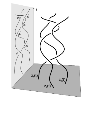
Figure 1: Braiding of three directed lines. Elementary moves $\sigma_{i}$ in the projection generate the group $B_{3}$.

In what follows we shall repeatedly use the so-called Burau matrix representation of the braid group. In the particular case of the group $B_{3}$ the Burau representation is given by $2\times 2$ matrices:

$$\sigma_{1}=\left(\begin{array}[]{cc}-t&1\\ 0&1\end{array}\right);\qquad\sigma_{2}=\left(\begin{array}[]{cc}1&0\\ t&-t\end{array}\right)$$ (1)

where $t$ is a free parameter. It is known that for $B_{3}$ this representation is faithful birman . When $t=-1$ the group $B_{3}$ coincides with the modular group $PSL(2,{\mathbb{Z}})$.

The paper is structured as follows. The first part introduces the basic notions of homotopy groups and homotopic length, necessary to self-contained description of topological invariants. The method proposed in this part, demonstrates on the simplest examples how the monodromy representations of groups allows one to build the universal coverings, giving rise to topological invariants, associated at a physical level to fluxes of non-Abelian extension of ”solenoidal magnetic fields”. Using the same ideas, the second part deals with the case of $B_{3}$ for which we explicitly derive a topological invariant, directly linked to the irreducible braid length, and construct its non-Abelian flat connection. For the model of ideal Brownian braids, the stochastic evolution of this topological invariant is given and its asymptotic distribution is derived.

II Topological invariants and monodromy representations

II.1 Basic concepts and definitions

Let us consider the double–punctured complex plane ${\mathbb{C}}^{\star\star}={{\mathbb{C}}}-\{z_{1},z_{2}\}$, of variable $z=x+iy$ and suppose the coordinates of the punctures $M_{1}$ and $M_{2}$ to be $z_{1}=(0,0)$ and $z_{2}=(c,0)$ correspondingly. We set $c\equiv 1$ by appropriate rescaling of the plane $z$.

Take now two closed elementary paths on $z$ such that the first one ($\gamma_{1}$) encloses only the point $M_{1}$ and the second one ($\gamma_{2}$) surrounds only the point $M_{2}$. With the usual composition law of paths, $\gamma_{1}$ and $\gamma_{2}$, generate a fundamental group $F_{2}$, which is the first homotopy group, $\pi_{1}$, of the double–punctured complex plane $z$:

$$\pi_{1}({\mathbb{C}}^{\star\star})=F_{2}$$

The trivial path (the unit element of the group $F_{2}$) is the composition of an arbitrary loop with its inverse: $e=\gamma_{i}\gamma_{i}^{-1}=\gamma_{i}^{-1}\gamma_{i},\;i=\{1,2\}$. The loops $\gamma_{i}$ and $\tilde{\gamma}_{i}$ are equivalent if $\gamma_{i}$ can be continuously deformed into $\tilde{\gamma}_{i}$ (the equivalent loops represent the same element of $F_{2}$). We denote the class of equivalent paths by $\gamma_{i}$.

Any element of the group $F_{2}$ being finitely generated, corresponds to a closed path on $z$ and can be represented by a ”word” consisting of a sequence of letters–generators of the group $F_{2}$: $\{\gamma_{1},\gamma_{2},\gamma_{1}^{-1},\gamma_{2}^{-1}\}$. Each word can be reduced to a minimal (or ”irreducible”) representation. For example, the word $W=\gamma_{1}\gamma_{2}^{-1}\gamma_{1}\gamma_{1}\gamma_{1}^{-1}\gamma_{2}^{-1}\gamma_{2}\gamma_{1}^{-1}\gamma_{2}^{-1}\equiv\gamma_{1}\gamma_{2}^{-1}\left[\gamma_{1}\left[\gamma_{1}\gamma_{1}^{-1}\right]\left[\gamma_{2}^{-1}\gamma_{2}\right]\gamma_{1}^{-1}\right]\gamma_{2}^{-1}$ can be reduced to $W=\gamma_{1}\gamma_{2}^{-1}\gamma_{2}^{-1}$. Consider now a finitely generated group $G=\langle g_{1},g_{2}\rangle$ (to be more precise, the group admitting only one– or two–generators presentation). We are interested in the monodromy representation of $F_{2}$ into $G$ defined by the following group homomorphism $\Psi$:

$$\Psi:\left\{\begin{array}[]{lll}F_{2}&\longrightarrow&G\\ \gamma_{i}&\longrightarrow&g_{i}\quad(i=1,2)\end{array}\right.$$ (2)

Note that this straightforwardly can be generalized to the case of multi–punctured surfaces or other topological spaces. We do not discuss in details the existence of such homomorphism, assuming that it results mainly from the fact that $F_{2}$ is a free group.

Our main goal in the present paper consists in defining an explicit geometrical construction of a non-Abelian generalization of a Gauss topological invariant (i.e. a ”linking number”) for different groups $G$ using the monodromy representations of $G$. In particular, we construct a complex flat connection $A(z)$ on ${\mathbb{C}}^{\star\star}$, i.e. a ”Bohm-Aharonov–like vector potential” $A(z)$, whose holonomy gives rise to a representation of $G$. A special attention is paid to the case when $G=B_{3}$. Moreover, we use the developed approach to estimate the averaged complexity of a 3–strand braid represented by independent motion of 3 Brownian particles in (2+1) dimensions.

II.2 Topological invariants from conformal maps

In order to explain the basic notions, we begin with the simplest possible case—the Abelian group ${\mathbb{Z}}$ and construct the corresponding topological invariant by means of conformal transforms.

II.2.1 Abelian case: commutative group $G={\mathbb{Z}}$

The central point of the approach deals with the reconstruction of a linear differential equation on the manifold ${\mathbb{C}}^{\star\star}$ by its monodromy group $G$. In other words, defining the action of $G$ on the space of solutions of some $2^{\rm nd}$–order liner differential equation with two branching points, we are attempting to recover the form of this differential equation and its solutions. In the case of $G={\mathbb{Z}}$ it is natural to consider a usual 1-dimensional additive action

$$n[w(z)]=w(z)+2i\pi n$$

for $w$ defined on ${\mathbb{C}}^{\star\star}$ and $n\in{\mathbb{Z}}$. It turns out that the simplest linear differential equation with two branching points, satisfying those conditions is:

$$(z-z_{1})(z-z_{2})\frac{dw}{dz}-2z+z_{1}+z_{2}=0$$ (3)

whose solution reads

$$w(z)=\ln(z-z_{1})+\ln(z-z_{2})$$ (4)

One can check that the free group $\Gamma_{2}$ acts on the space of solutions as follows

$$w(z)\stackrel{{\scriptstyle\{\gamma_{1},\gamma_{2}\}}}{{\longrightarrow}}w(z)+2i\pi$$ (5)

which means that the homomorphism $\Psi$ is trivial in for this example: $\Psi(\gamma_{i})=1$ $(i=1,2)$. The function $w(z)$ conformally maps the doubly punctured plane to the universal covering space $w=u+iv$ free of any branching points. In the complex plane $w$ we have

$$\left\{\begin{array}[]{l}u=\ln|(z-z_{1})(z-z_{2})|\vskip 6.0pt plus 2.0pt minus 2.0pt\\ v=\arg(z-z_{1})+\arg(z-z_{2})\end{array}\right.$$

The function $w(z|z_{1},z_{2})$ is a topological invariant because of equality (5). In particular, the function $v(z|z_{1},z_{2})$ defines the total number of turns in the plane $z$ around the branching points $z_{1}$ and $z_{2}$ and hence it is nothing else as the Gauss linking number.

Thus, knowing the conformal transform $w(z)$ of the multiply punctured plane ${\mathbb{C}}^{\star\star}$ to the universal (i.e. uniformizing) covering surface, we can easily extract a topological invariant ${\rm Inv}(\gamma)$ of a closed path $\gamma$ (starting and ending at some arbitrary point $z_{0}\neq\{0,1\}$ in the plane $z$) from the difference $w_{\rm in}(z_{0})-w_{\rm fin}(z_{0})$. The path $\gamma$ connects the images of the point $z_{0}$ on different Riemann sheets—the ”copies” of the fundamental domain of $G$. Recall that by definition the fundamental domain of a group $G$ is a minimal connected domain tessellating the whole covering space under the action of $G$. Representing the topological invariant ${\rm Inv}_{(z)}(\gamma)$ as a full derivative along the contour $\gamma$, we get:

$${\rm Inv}_{(z)}(\gamma)\stackrel{{\scriptstyle\rm def}}{{=}}w_{\rm fin}-w_{\rm in}\equiv\oint\limits_{\gamma}\frac{dw(z)}{dz}dz=\oint A(z)dz$$ (6)

The physical interpretation of the derivative $A(z)=\frac{dw(z)}{dz}$ is very straightforward. The conformal transform $w(z)$ plays the role of a complex potential of a field $A(z)$, which defines a flat connection of a multiple–punctured plane ${{\mathbb{C}}}^{\star\star}$.

For the commutative group $G={\mathbb{Z}}$ we obtain $A(z)$ by taking the derivative of (4):

$$A(z)=\frac{1}{z-z_{1}}+\frac{1}{z-z_{2}}$$ (7)

This expression can be easily identified with the standard (Abelian) Bohm–Aharonov vector potential of two solenoidal magnetic fields orthogonal to the plane $z$ and crossing it in the points $z_{1}$ and $z_{2}$.

In the next section the same construction of the flat connection associated to a specific group $G$ will be generalized to the non-Abelian case.

II.2.2 Non-Abelian case: non-commutative groups $F_{2},\,H_{q}$

We consider a special class of hyperbolic and hyperbolic–like groups: the free ($F_{2}$) and the Hecke ($H_{q}$) groups, as well as the braid group $B_{3}$. By hyperbolic–like groups we mean a class broader than hyperbolic groups in the classification of M.Gromov gromov . (According to the Gromov’s definition, the group $B_{3}$ does not belong to the class of hyperbolic groups). The important feature for us would be just the exponential growth of the group. From this point of view the group $B_{3}$ fits our scheme.

1. The free group $F_{2}$ (in general, $F_{n}\;(n=2,3,4,...)$) by definition is the free product of two (in general of $n$) copies of cyclic groups of second order, ${{\mathbb{Z}}}_{2}$. The matrix representation of the generators of the free groups $F_{2}\{f_{1},f_{2}\}$ and $F_{3}\{f_{1},S\}$ are:

$$\begin{array}[]{l}F_{2}:\quad f_{1}=\left(\begin{array}[]{cc}1&2\\ 0&1\end{array}\right);\;f_{2}=\left(\begin{array}[]{cc}1&0\\ 2&1\end{array}\right)\vskip 6.0pt plus 2.0pt minus 2.0pt\\ F_{3}:\quad f_{1}=\left(\begin{array}[]{cc}1&2\\ 0&1\end{array}\right);\;S=\left(\begin{array}[]{cc}0&1\\ -1&0\end{array}\right)\end{array}$$ (8)

2. The Hecke group $H_{q}$ is the free product of two cyclic groups ${\mathbb{Z}}_{2}$, and ${\mathbb{Z}}_{q}$ of orders 2 and $q$ respectively. The Hecke group is defined by the relations

$$\begin{array}[]{r}(ST_{q})^{q}=b_{q}^{q}=1\vskip 6.0pt plus 2.0pt minus 2.0pt\\ S^{2}=a_{2}^{2}=1\end{array}$$ (9)

where the generators $T_{q}$ and $S$ have the following matrix representation

$$H_{q}:\quad T_{q}=\left(\begin{array}[]{cc}1&2\cos\frac{\pi}{q}\\ 0&1\end{array}\right);\;S=\left(\begin{array}[]{cc}0&1\\ -1&0\end{array}\right)$$ (10)

The parameter $q$ takes discrete values $q=3,4,5,6,\ldots$. The Hecke group $H_{q}$ ”interpolates” between the modular group $PSL(2,{\mathbb{Z}})$ (for $q=3$) and the free group $F_{3}$ with 3 generators ($q\to\infty$).

We have stressed in the previous section that the topological invariant can be constructed on the basis of the conformal map $w(z)$ of multiple–punctured plane to the universal covering space of a group. We now extend the described method to more interesting cases than considered at length of the section II.2.1.

We derive the conformal mapping of the half–plane ${\rm Im}\,z>0$ onto the fundamental domain of the triangular group $G$—a curvilinear triangle lying in the upper half–plane ${\rm Im}\,w>0$. The action of $G$ on this fundamental domain generates the whole covering space. Each copy of the fundamental domain represents a Riemann sheet corresponding to the fibre bundle above $z$ and the whole covering space $w$ is the unification of all such Riemann sheets—see fig.2.

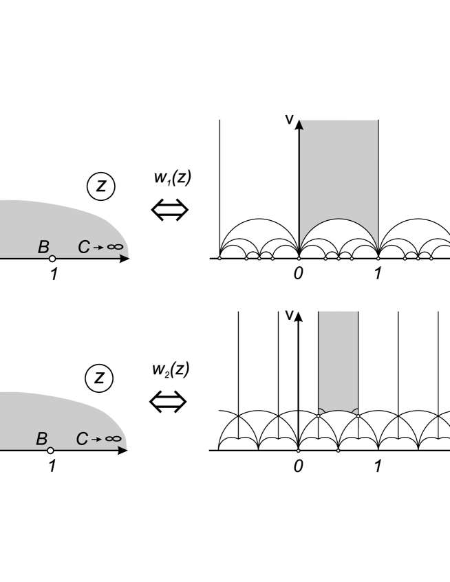
Figure 2: Conformal transforms of the upper half-plane ${\rm Im}\,z>0$ to the fundamental domain of the group $F_{2}$ (up) and of the group ${PSL(2,{\mathbb{Z}})}$ (down).

The coordinates of initial and final points of a trajectory on the universal covering $w$ determine:

• The coordinates of the corresponding points on $z$;

• The element of $G$ corresponding to the homotopy class of the path on $z$.

Following the construction described in the previous section let us define the action of $G\{g_{1},g_{2}\}$ in the complex plane $w=u+iv$. The group $G$ admits the faithful 2–dimensional representations and acts in the covering space $w$ by fractional–linear transforms. Consider two basic contours $\gamma_{1}$ and $\gamma_{2}$, associated to the action of $G$ on $z$ ($z\neq\{z_{1},z_{2},\infty\}$. The contours $\gamma_{1}$ and $\gamma_{2}$ enclose the branching points located at $z_{1}$ and $z_{2}$ correspondingly ($z\neq\{z_{1},z_{2},\infty\}$). The function $w(z)$ ($z\neq\{z_{1},z_{2},\infty\}$) obeys the following transformations:

$$w\left[z\stackrel{{\scriptstyle\gamma_{1}}}{{\rightarrow}}z\right]\rightarrow\tilde{w}_{1}(z)=\frac{a_{1}w(z)+b_{1}}{c_{1}w(z)+d_{1}};\quad w\left[z\stackrel{{\scriptstyle\gamma_{2}}}{{\rightarrow}}z\right]\rightarrow\tilde{w}_{2}(z)=\frac{a_{2}w(z)+b_{2}}{c_{2}w(z)+d_{2}}$$ (11)

The matrices $g_{1}$ and $g_{2}$

$$g_{1}=\left(\begin{array}[]{cc}a_{1}&b_{1}\\ c_{1}&d_{1}\end{array}\right);\qquad g_{2}=\left(\begin{array}[]{cc}a_{2}&b_{2}\\ c_{2}&d_{2}\end{array}\right)$$ (12)

are the matrices of basic substitutions of the group $G\{g_{1},g_{2}\}$, i.e. $g_{1}$ and $g_{2}$ are the generators of $G$.

It is well known that the function $w(z)$ can be defined as the quotient of two fundamental solutions $u_{1}(z)$ and $u_{2}(z)$ of a second order differential equation with branching points $\{z_{1}=(0,0),z_{2}=(0,1),z_{3}=\infty\}$. As it follows from the analytic theory of differential equations, the solutions $u_{1}(z)$ and $u_{2}(z)$ undergo the linear substitutions when the variable $z$ moves along the contours $\gamma_{1}$ and $\gamma_{2}$:

$$\gamma_{1}:\,\left(\begin{array}[]{c}\tilde{u}_{1}(z)\\ \tilde{u}_{2}(z)\end{array}\right)=g_{1}\left(\begin{array}[]{c}u_{1}(z)\\ u_{2}(z)\end{array}\right);\quad\gamma_{2}:\,\left(\begin{array}[]{c}\tilde{u}_{1}(z)\\ \tilde{u}_{2}(z)\end{array}\right)=g_{2}\left(\begin{array}[]{c}u_{1}(z)\\ u_{2}(z)\end{array}\right)$$ (13)

where $g_{1}$ and $g_{2}$ are the generators of the monodromy group of this equation. The problem of restoring the form of a differential equation by the monodromy matrices $g_{1}$ and $g_{2}$ of the group $G$ of the differential equation, is known as the Riemann-Hilbert problem. Yet we restrict ourselves with the groups $F_{2}$ and $H_{q}$, the group $B_{3}$ shall be considered separately.

The free group $F_{2}$. For the free group $F_{2}$ the solution of the Riemann-Hilbert problem gives rise to the following second–order differential equation bateman :

$$z(z-1)\frac{d^{2}u(z)}{dz^{2}}+(2z-1)\frac{du(z)}{dz}+\frac{1}{4}u(z)=0$$ (14)

Indeed, a possible basis of solutions of this equation is as follows:

$$\left\{\begin{array}[]{ll}u_{1}(z)=F(1/2,1/2,1,z)\vskip 6.0pt plus 2.0pt minus 2.0pt\\ u_{2}(z)=iF(1/2,1/2,1,1-z)\end{array}\right.$$ (15)

Using the well–known properties of hypergeometric functions, one can restore the monodromy matrices defined in (13) for this basis:

$$g_{1}=\left(\begin{array}[]{cc}1&0\\ 2&1\end{array}\right);\qquad g_{2}=\left(\begin{array}[]{cc}1&-2\\ 0&1\end{array}\right)$$ (16)

which coincides with the generating set of the group $F_{2}$. The function $w(z)$ performing the conformal map of the upper half–plane Im$z>0$ onto the fundamental domain (the curvilinear triangle $ABC$) of the universal covering $w$ satisfies eq.(11) and can be written as:

$$w(z)=\frac{u_{1}(z)}{u_{2}(z)}$$ (17)

The function $w(z)$ is well known in the literature (see, for example, bateman ) and its inverse $z(w)$ is the elliptic modular function

$$z(w)\equiv\lambda(w)=\frac{\theta_{2}^{4}(0,w)}{\theta_{3}^{4}(0,w)}$$ (18)

Now we can give an explicit expression of the flat connection ${\bf A}(z)$ for the doubly punctured plane corresponding to the monodromy of the free group $F_{2}$. Taking the derivatives and using the properties of the hypergeometric functions, we get:

$$A(z)=\frac{dw(z)}{dz}=-i\frac{E(z)K(1-z)+(E(1-z)-K(1-z))K(z)}{2z(z-1)K^{2}(1-z)}$$ (19)

where

$$K(z)=\int\limits_{0}^{\pi/2}\frac{d\theta}{\sqrt{1-z\sin^{2}\theta}};\qquad E(z)=\int\limits_{0}^{\pi/2}d\theta\sqrt{1-z\sin^{2}\theta}$$ (20)

are correspondingly the complete elliptic integrals $K(z)$ and $E(z)$ (see, for example, abramowitz ).

In the Fig.3 we have plotted the absolute values $|A(z)|$ of the Abelian (Eq.(7)) and the non-Abelian (Eq.(19)) flat connections.

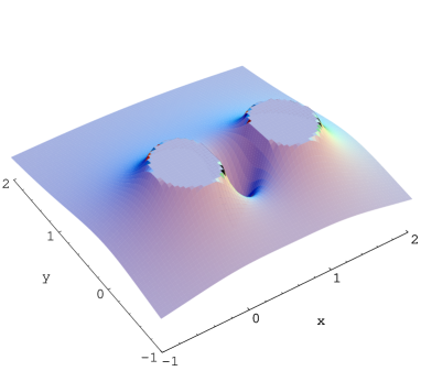
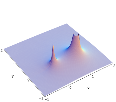
Figure 3: The cuts of the function $|A(z)|$ in the Abelian (left) and non-Abelian (right) cases.

The leading asymptotics of (19) are as follows:

$$A(z)\sim\left\{\begin{array}[]{cl}\displaystyle\frac{-i\pi}{z\ln^{2}z}&\quad\mbox{as $z\to 0$}\vskip 6.0pt plus 2.0pt minus 2.0pt\\ \displaystyle\frac{-i}{\pi(z-1)}&\quad\mbox{as $z\to 1$}\end{array}\right.$$ (21)

Hence even in the vicinity of the branching point $z=0$ the function $A(z)$ defined in (19) does not coincide asymptotically with the flat connection for the Abelian case (7).

The Hecke group $H_{q}$. We now pass to the case of $H_{q}$, keeping in mind that for $q=3$ we recover the group $PSL(2,{\mathbb{Z}})$, directly linked to $B_{3}$ ($B_{3}$ is a central extension of $PSL(2,{\mathbb{Z}})$, see birman ). The solution of the corresponding Riemann-Hilbert problem leads to the following differential equation: venkov

$$z(z-1)\frac{d^{2}u(z,q)}{dz^{2}}+\left[\left(\frac{3}{2}-\frac{1}{q}\right)z-\left(1-\frac{1}{q}\right)\right]\frac{du(z,q)}{dz}+\frac{1}{4}\left(\frac{1}{2}-\frac{1}{q}\right)^{2}u(z,q)=0$$ (22)

whose possible basis of solution is:

$$\left\{\begin{array}[]{ll}\displaystyle u_{1}(z)=F\left(\frac{q-2}{4q},\frac{q-2}{4q},1-\frac{1}{q},z\right)-\lambda(q)e^{i\pi/q}z^{1/q}F\left(\frac{q+2}{4q},\frac{q+2}{4q},1+\frac{1}{q},z\right)\vskip 6.0pt plus 2.0pt minus 2.0pt\\ \displaystyle u_{2}(z)=-e^{i\pi/q}F\left(\frac{q-2}{4q},\frac{q-2}{4q},1-\frac{1}{q},z\right)+\lambda(q)z^{1/q}F\left(\frac{q+2}{4q},\frac{q+2}{4q},1+\frac{1}{q},z\right)\end{array}\right.$$ (23)

where

$$\lambda(q)=\displaystyle e^{2i\pi/q}\frac{\Gamma(1-\frac{1}{q})\Gamma(\frac{q+2}{4q})\Gamma(\frac{3q+2}{4q})}{\Gamma(1+\frac{1}{q})\Gamma(\frac{q-2}{4q})\Gamma(\frac{3q-2}{4q})}$$ (24)

Taking into account that the series defining the hypergeometric functions $F(z)$ converges for $|z|<1$ and corresponds to the so-called logarithmic case (see bateman ) one obtains from (23) the following monodromy matrices after proper analytic continuation:

$$g_{1}=e^{i\pi/q}\left(\begin{array}[]{cc}2\cos\frac{\pi}{q}&1\\ -1&0\end{array}\right);\qquad g_{2}=i\left(\begin{array}[]{cc}0&-1\\ 1&0\end{array}\right)$$ (25)

One can check that after normalization by the determinant, the matrices (25) become the generators of $H_{q}$ (correspondingly of orders $q$ and 2). Let us point out that for $q=3$, one can identify the inverse function $z(w)$ with the Klein’s ”absolute modular invariant”

$$z(w)\equiv J(w)=\frac{(\theta_{2}^{8}(0,w)+\theta_{3}^{8}(0,w)+\theta_{4}^{8}(0,w))^{3}}{54\theta_{2}^{8}(0,w)\theta_{3}^{8}(0,w)\theta_{4}^{8}(0,w)}$$

where $\theta_{2},\theta_{3},\theta_{4}$ are the Jacobi elliptic $\theta$–functions. As in the previous section, the corresponding complex flat connection $A_{H_{q}}(z)$ can be obtained as the full derivative

$$A_{H_{q}}(z)=\frac{dw_{H_{q}}(z)}{dz}$$

from the conformal map

$$w_{H_{q}}(z)=\frac{u_{1}(z)}{u_{2}(z)}$$

with $u_{1}(z)$ and $u_{2}(z)$ defined in (23).

III Invariant of 3-strand braids

Let us return to the model of random braids discussed in the very beginning of the paper. The system of three independently moving particles is described by 3 complex variables (i.e. 6 degrees of freedom) and hence our system can not be directly viewed as a monodromy problem. In order to describe the whole system by one complex variable $\zeta$ and to be able to use the tools elaborated in the previous section, with the minimal loss of information, we introduce the anharmonic quotient:

$$\zeta(t)=\frac{z_{23}(t)}{z_{13}(t)}\equiv\frac{z_{2}(t)-z_{3}(t)}{z_{1}(t)-z_{3}(t)}$$ (26)

One can easily check that the variable $\zeta$ contains the complete topological information of a mutual configuration of three entangled lines, except the global phase, or global twist of the braid. It means that we do not take into account the center of $B_{3}$ considering the factor group ${PSL(2,{\mathbb{Z}})}=B_{3}/{{\mathbb{Z}}}$. We can always take into account the global twist afterwards by passing to the rotating coordinate system with the origin located in the center of mass of the system of three particles. From the statistical point of view the possibility of neglecting the center of $B_{3}$ (which is equivalent to considering the factor group $PSL(2,{\mathbb{Z}})$ only), has been discussed in the papers raf ; voitnech3 . In fact, in these paper it has been shown that the escape rates for random walks on $B_{3}$ and $PSL(2,{\mathbb{Z}})$ are the same in the limit of infinitely long trajectories.

Thus, the parametrization of the three-particle system $\{z_{1}(t),\,z_{2}(t),\,z_{3}(t)\}$ by the function $\zeta(t)$ living in the doubly punctured complex plane enables us to preserve all topological characteristics of the braid of mutually entangled world lines of these particles. However the precise derivation of the expression for the flat connection, as it is shown below, explicitly depends on the fact whether the particles are identical or not.

Looking at the elementary moves associated with the generators $\sigma_{1},\ \sigma_{2}$ of $B_{3}$, we obtain the transformations for the variable $\zeta$. For example, let us pick up some path in the homotopy class of $\sigma_{1}$ (see fig.1). By definition of $\sigma_{1}$, we have at some time $t$:

$$\sigma_{1}[z_{1}\leftrightarrow z_{2},z_{3}\leftrightarrow z_{3}]:\left\{\displaystyle\begin{array}[]{lll}\displaystyle z_{1}(t)=\frac{z_{1}+z_{2}}{2}+\frac{1}{2}z_{12}e^{-i\pi t}\vskip 6.0pt plus 2.0pt minus 2.0pt\\ \displaystyle z_{2}(t)=\frac{z_{1}+z_{2}}{2}-\frac{1}{2}z_{12}e^{-i\pi t}\vskip 6.0pt plus 2.0pt minus 2.0pt\\ z_{3}(t)=z_{3}\end{array}\right.$$ (27)

In the same way we can get the transformation of $\zeta$ along a path corresponding to the homotopy class $\sigma_{2}\equiv\sigma_{2}[z_{1}\leftrightarrow z_{1},z_{2}\leftrightarrow z_{3}]$. Finally we arrive at the following set of transformations of $\zeta$:

$$\begin{array}[]{lcc}\displaystyle\sigma_{1}:\,\zeta&\to&\displaystyle\frac{1}{\zeta}\vskip 6.0pt plus 2.0pt minus 2.0pt\\ \displaystyle\sigma_{2}:\,\zeta&\to&\displaystyle\frac{\zeta}{\zeta-1}\end{array}$$ (28)

which precisely define the representation of the symmetric group $S_{3}$.

Indistinguishable particles. Our main goal consists in constructing the flat connection for the system of three identical particles moving in the plane. The condition of the indistinguishability of particles requires to factor the action of the group $B_{3}$ by $S_{3}$, and hence to consider $\zeta$ as living in the factor space ${\mathbb{C}}^{\star\star}/S_{3}$. The case of distinguishable particles shall be discussed at the end of this section.

All the trajectories $\zeta(t)$ (parameterized by $t$) are obviously closed in the space ${\mathbb{C}}^{\star\star}/S_{3}$. Keeping in mind our strategy of the previous section, we want to define a monodromy representation of $B_{3}$ (more precisely of $PSL(2,{\mathbb{Z}})$) acting on ${\mathbb{C}}^{\star\star}/S_{3}$. To do that we construct a conformal map $w_{s}(\zeta)$ of the doubly punctured plane factorized over the action of the symmetric group, ${\mathbb{C}}^{\star\star}/S_{3}$ onto the fundamental domain of the modular group, $PSL(2,{\mathbb{Z}})$:

$$w_{s}(\zeta):\,{\mathbb{C}}^{\star\star}/S_{3}\longrightarrow PSL(2,{\mathbb{Z}})$$ (29)

To our knowledge, the explicit method of solving the uniformization problem (29) has not been yet considered in the context of our problem. So, our own way to tackle it deals with the following observation.

Consider the so-called pure braid group $P_{3}$ defined as follows:

$$P_{3}=\langle\sigma_{1}^{2},\sigma_{2}^{2},(\sigma_{1}\sigma_{2})^{2}\rangle$$ (30)

It is obvious that the group $P_{3}$ is the subgroup of $B_{3}$. In particular, the group $P_{3}$ can be identified with the factor group $F_{2}\times{\mathbb{Z}}$ through the obvious correspondence

$$\sigma_{1}^{2}=g_{1},\;\sigma_{1}^{2}=g_{1}$$ (31)

where $g_{1}$ and $g_{2}$ are the generators of the free group $F_{2}$. The relations (14) follow from the Burau representation of braid group generators (1) and the obvious geometric construction shown in the fig.4.

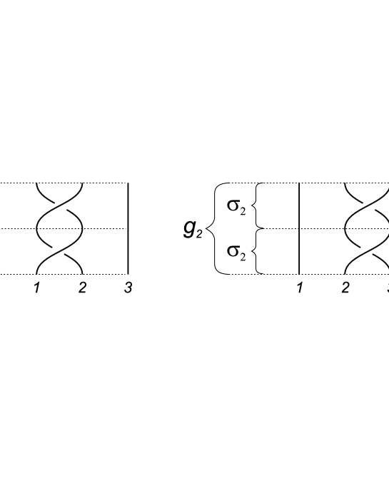
Figure 4: The squares of the braid group generators $\sigma_{i}$ act as the free group generators $g_{i}$: $g_{i}=\sigma_{i}^{2}$ ($i=1,2$).

In the case of the pure braid group $P_{3}$ there is no difference between distinguishable and indistinguishable particles moving in the plane $z$ because the generators $g_{1}$ and $g_{2}$ correspond to ”full turns” of one world line of the particle with respect to another one (and not to ”half turns” as in case of the braid group $B_{3}$). That is, we deal with the monodromy representation of $F_{2}$. Let us remind that we factor out the global turns (i.e. the center of the group) in the space ${\mathbb{C}}^{\star\star}$. The uniformization problem in this case is solved by the conformal map $w_{s}(\zeta)$ of the doubly punctured plane to the covering space

$$w_{s}(\zeta):\,{\mathbb{C}}^{\star\star}\longrightarrow F_{2}$$

Thus, we return to the topic of the previous section, where an explicit form of such conformal map $w_{s}(\zeta)\equiv w(\zeta)$ is given in (17).

Consider now the whole group $B_{3}/{\mathbb{Z}}$, take the same function $w(\zeta)$ and check the effect of the basic substitutions of the symmetric group (28) onto the transformations of $w(\zeta)$. Using the well known properties of the modular functions (see, for example, hille ; golubev ; mckay ), we get:

$$\left\{\begin{array}[]{lcc}\displaystyle w_{s}\left(\zeta\to\frac{1}{\zeta}\right)&\to&\displaystyle-w_{s}+1\vskip 6.0pt plus 2.0pt minus 2.0pt\\ \displaystyle w_{s}\left(\zeta\to\frac{\zeta}{\zeta-1}\right)&\to&\displaystyle\frac{w_{s}}{w_{s}-1}\end{array}\right.$$ (32)

The transformations of $w_{s}$ precisely coincide with the basic transformations of the modular group $PSL(2,{\mathbb{Z}})$. In fact, technically it is much easier to check (instead of (32)) the transformations for the inverse function $\zeta(w_{s})=\frac{\theta_{2}^{4}(0,w_{s})}{\theta{(0,w_{s})}}$:

$$\left\{\begin{array}[]{lcc}\displaystyle\zeta\left(w_{s}\to-w_{s}+1\right)&\to&\displaystyle\frac{1}{\zeta}\vskip 6.0pt plus 2.0pt minus 2.0pt\\ \displaystyle\zeta\left(w_{s}\to\frac{w_{s}}{w_{s}-1}\right)&\to&\displaystyle\frac{\zeta}{\zeta-1}\end{array}\right.$$ (33)

Hence the function $w_{s}(\zeta)$ explicitly solves the desired uniformization problem (29). Thus, we can use this function $w_{s}(\zeta)$ to construct the non-Abelian flat connection $A_{s}(\zeta)$ for the trajectories on ${\mathbb{C}}^{\star\star}/S_{3}$ parametrized by $\zeta(t)$:

$$A_{s}(\zeta)=\frac{dw_{s}(\zeta)}{d\zeta}$$ (34)

where

$$w_{s}(\zeta)\equiv w(\zeta)=\frac{u_{1}(\zeta)}{u_{2}(\zeta)}=-i\,\frac{F(1/2,1/2,1,z)}{F(1/2,1/2,1,1-z)}$$

(see eq.(15)).

The expression (34) is the source for the explicit construction of the topological invariant via equation (6) of three entangled world lines $z_{1}(t)$, $z_{2}(t)$ and $z_{3}(t)$ shown in fig.1.

Distinguishable particles. For distinguishable particles the action of the symmetric group $S_{3}$ should be neglected and hence $\zeta$ is living in the doubly punctured plane, ${\mathbb{C}}^{\star\star}$. The problem of uniformization in this case is solved by the conformal map $w_{d}(\zeta)$ mapping the doubly punctured plane, ${\mathbb{C}}^{\star\star}$, onto the fundamental domain of the modular group, $PSL(2,{\mathbb{Z}})$:

$$w_{d}(\zeta):\,{\mathbb{C}}^{\star\star}\longrightarrow PSL(2,{\mathbb{Z}})$$ (35)

(compare this expression to (29)). The corresponding function $w_{d}(\zeta)$ coincides with $w_{2}(\zeta)=\frac{u_{1}(\zeta)}{u_{2}(\zeta)}$ found in the privious section (use the equations (23)–(24) for $q=3$).

IV Stochastic behavior of the invariant for Brownian 3-strand braids

We are interested in this section in the stochastic behavior of the invariant $|w(\eta)|$ when each of the three particles perform a 2D Brownian motion (BM) represented by its complex coordinate $z_{i}$. This model naturally appears as the generalization of the Edwards’ problem of determining the distribution of the winding angle of two independent 2D BM edwards . The intrinsic noncommutative structure of the 3–particles model, contrary to the commutative 2–particles problem, induces a completely different behavior of the invariant, which characterizes quantitatively the tangle complexity. The method employed here is inspired by a work of Gruet gruet .

IV.1 The Ideal Model

We begin with an ideal case of point–like particles diffusing in the infinite plane with the diffusion constants $D$ set to 1. Following previous sections, one has to study the motion of the reduced variable $\eta$ in the space ${\mathbb{C}}^{\star\star}/S_{3}$. Our strategy relies on the following theorem on conformal transforms of complex BM often referred to as a generalized Paul Lévy’s theorem yor . Denote by $B_{t}$ the generic BM in the complex plane $z$. For any conformal map $f$, the image $Y_{t}=f(B_{t})$ of a BM $B_{t}$ is a time changed BM $B_{u}(t)$ such that

$$du=\dfrac{1}{4}dYd\bar{Y}=|f^{\prime}(B_{t})|^{2}dt$$ (36)

In terms of the diffusion equation (which corresponds to the Langevin equation (36), the time change can be interpreted as a space dependent diffusion coefficient ito-mckean :

$$\partial_{t}P(Y_{t})=\dfrac{du}{dt}\Delta P(Y_{t})$$ (37)

A slightly modified version of the generalized Lévy theorem shows that $\zeta(t)$, being the ratio of two complex BM (see (26)), is also a time changed BM, denoted $\zeta(t)=B_{u(t)}$. The time change then reads, following the rules of Itô calculus:

$$du=\frac{1}{4}d\zeta d\bar{\zeta}=\frac{1+|\zeta(t)|^{2}}{|z_{32}(t)|^{2}}dt$$ (38)

Now we should pass to the covering space $w$ and describe the evolution of the invariant $w(\zeta)=w(B_{u})$. Using once more the generalized Lévy’s theorem, we obtain that there exists a hyperbolic BM $\tilde{B}$ such that $w(\zeta)$ is again a time–changed $\tilde{B}$:

$$w(\zeta(t))=\tilde{B}_{\tau(u(t))}$$ (39)

with

$$d\tau=\dfrac{|w^{\prime}(B_{u})|^{2}}{{\rm Im}^{2}(w(B_{u}))}du$$ (40)

The choice of the hyperbolic metric is not artificial and anticipates the geometrical properties of the transform $w(\zeta)$. Note the importance of obtained result: we know that the topological invariant $w(\zeta)$, giving the braid complexity, performs a hyperbolic diffusion in a new time, or equivalently a hyperbolic diffusion in a space with the metric–dependent diffusion coefficient. We now have to study the full time change $\tau(t)$. Combining (38) and (40) and using the well known inverse function $w^{-1}\equiv z(w)=\lambda(w)$ (see (18)), we obtain after separating the variables the following implicit relation between $t$ and $\tau$, which defines the functional $H_{t}(\tau)$:

$$H_{t}(\tau)=\int_{0}^{t}\frac{dt^{\prime}}{|z_{32}(t^{\prime})|^{2}}=\int_{0}^{\tau}\frac{|\lambda^{\prime}(\tilde{B}_{\tau^{\prime}})|^{2}}{1+|\lambda(\tilde{B}_{\tau^{\prime}})|^{2}}{\rm Im}^{2}(\tilde{B}_{\tau^{\prime}})d\tau^{\prime}$$ (41)

This expression is exact, but does not allow a straightforward interpretation. Let us first notice that the $t$–dependence can be easily shown to be, with the probability one:

$$\lim_{t\to\infty}\frac{H_{t}(\tau)}{\ln t}=C_{1}>0$$ (42)

The sensitive point is the $\tau$–dependence. The integral kernel $f$

$$f:\;z\longrightarrow\frac{|\lambda^{\prime}(z)|^{2}}{1+|\lambda(z)|^{2}}{\rm Im}^{2}(z)$$ (43)

is invariant under the transformations of the group $F_{2}$, and $H_{t}(\tau)$ is therefore an additive functional of the BM on the quotient surface ${\mathbb{H}}/F_{2}$. This motion is ergodic. Therefore if $H_{t}(\tau)$ is integrable over the fundamental domain of $F_{2}$, one can clear up the asymptotic $\tau$–dependence (see in particular a similar approach proposed by Gruet in gruet ). In our case $H_{t}(\tau)$ is not integrable over the domain of $F_{2}$; the $\tau$–dependence for this ideal model requires more attention and have to be treated with more care. We expect to consider that question in details separately, while below we express a conjecture based on the fact that the non-integrability does not lead to a growth faster than $\tau$. We indeed believe that the non-integrability gives rise to sub-leading terms in $\tau$ and the following limit holds:

$$\lim_{\tau\to\infty}\frac{H_{t}(\tau)}{\tau}=C_{2}$$ (44)

Comparing (42) and (44) we arrive at the relation

$$\lim_{t\to\infty}\frac{\tau(t)}{t}=\frac{C_{1}}{C_{2}}$$ (45)

Using (45) we formulate a central result connecting the hyperbolic BM $\tilde{B}_{\tau}$ describing the connection of the expectation of our topological invariant $d(w)$ being the distance in the covering space $w$, with the word length $L(\tilde{B}_{\tau})$ of the corresponding random braid. Recall that the distribution of $\tilde{B}_{\tau}$ is well known, and in particular,

$$\lim_{\tau\to\infty}\frac{d(\tilde{B}_{\tau})}{\tau}=1$$

almost surely. Moreover, if one notices that the word lengths $L$ for $PSL(2,{\mathbb{Z}})$ and for $F_{2}$ are quasi-isometric, we have:

$$\lim_{\tau\to\infty}\frac{\left<L(\tilde{B}_{\tau})\right>}{\tau\ln\tau}=C_{3}>0\quad\mbox{in probability}$$ (46)

what is a direct consequence of a theorem by Gruet proved in gruet . Combining this result with (45, we end up with the following leading asymptotics at large time for the expectation of the word length of Brownian 3–strand braids:

$$\left\langle L_{t}\right\rangle\sim\ln(t)\times\ln(\ln t)\quad\mbox{for $t\to\infty$}$$ (47)

The average topological complexity increases with time, however the growth is very slow. It is limited (as in the case of two particles where this logarithmic scaling also holds) by the angular part of the 2D BM in an infinite space ito-mckean ; edwards2 : when two particles are far apart (and the corresponding typical distance grows with time), their relative angle varies very slowly.

IV.2 Model with a compact domain

We here discuss the physical reasons that justify a regularization of the integral (41) over the fundamental domain of $F_{2}$. The divergence of this integral occurs when $\eta$ approaches the points $\{0,1,\infty\}$ meaning that either two particles collide, or one particle goes to infinity. It is then quite natural to modify slightly the model in order to avoid these pathological cases, which in fact are not realistic if one describes the physical objects of finite thickness such as polymers. Specifically, we assume that three Brownian particles evolve in a bounded domain of characteristic size $R$ and that they experience hard-core repulsion at distance $r$. This can be re-expressed in terms of constraints due to hard walls added to the domain of $\eta$, hereafter denoted by $D$:

$$\begin{array}[]{ll}\epsilon(r,R)\leq|\eta|\leq M(r,R)\vskip 6.0pt plus 2.0pt minus 2.0pt\\ |\eta(r,R)-1|\geq\epsilon\end{array}$$ (48)

The precise shape of the boundary of $D$ is not important. Note that $w(D)$ is compact in ${\mathbb{H}}$. Restricting our model to this domain, we can now claim the integrability of the functional $H^{D}_{t}(\tau)$ over the domain $w(D)$. Within this approximation, we obtain the following $\tau$–dependence from the ergodic property offered above:

$$\lim_{\tau\to\infty}\frac{H^{D}_{t}(\tau)}{\tau}=C_{4}>0$$ (49)

In this model the $t$–dependence is readily changed as follows:

$$\lim_{t\to\infty}\frac{H^{D}_{t}(\tau)}{t}=C_{5}>0$$ (50)

Comparing (49) and (50) we arrive at

$$\lim_{t\to\infty}\frac{\tau(t)}{t}=\frac{C_{4}}{C_{5}}$$ (51)

The expectation of $d(w)$ can now be described asymptotically: $d(w)$ is a hyperbolic BM in the variable $\tau\propto t$ (see (51)). In particular, we have with the probability one:

$$\lim_{t\to\infty}\frac{\left<d(w(\eta))\right>}{t}=C_{6}>0$$ (52)

For a compact domain one can straightforwardly check that the topological invariant, $d$, and the word length, $L$, are quasi-isometric. The asymptotic behavior of the expectation value of $L$ is therefore similar to the one of $\left<d(w(\eta))\right>$:

$$\left\langle L_{t}^{D}\right\rangle\sim t\quad\mbox{for $t\to\infty$}$$ (53)

For the bounded domain, the topological complexity grows much faster, as the infinite space effect discussed above is absent. The scaling $\left<L_{t}^{D}\right>\propto t$ should be compared to the (commutative) scaling $\left<L_{\rm comm}\right>\propto\sqrt{t}$ for two particles. It is noteworthy to stress that (53) is fully consistent with a discrete model considered in voitnech3 ; raf .

V Conclusion

To conclude, we would like to comment the new physical content of our results. So far the only topological invariant studied in the context of entanglements of fluctuating linear objects was the so-called winding number belisle ; alain1 ; nelson ; kardar , which is known to be incomplete for more than two linear objects. We here propose a model, which describes exactly the underlying non-Abelian topology of the problem.

We propose a simple geometrical construction of topological invariants of 3–strand Brownian braids viewed as world lines of 3 particles performing independent Brownian motions in the complex plane $z$. Our construction is based on the properties of conformal maps of doubly-punctured plane $z$ to the universal covering surface. We pay special attention to the case of indistinguishable particles. Our approach is mainly ”self made” and its geometrical transparency we consider as the basic advantage. The standard machinery of constructing the nontrivial braid group representations from the Conformal Field Theory is outlined in the Appendix where we mainly review the strategy realized in todorov . The Appendix is added to our paper exclusively to establish some links between the approachs based on the geometry of conformal maps and on CFT.

Our method of conformal maps allow us to investigate the statistical properties of the topological complexity of a bunch of 3–strand Brownian braids and to compute the expectation value of the irreducible braid length.

Appendix A Braid group representation and CFT

In this section we try to describe the derivation of the braid group representation from the monodromies of some CFT. We will mainly describe the system under investigation in physical terms, rather than in more rigorous but less transparent algebraic topological setting.

So, consider $n$ ($n=3$ shall be mainly treated) indistinguishable particles, living in the complex plane ${\mathbb{C}}$. The ”static” (or configurational) phase space is the following set $X_{n}=Y_{n}/S_{n}={\mathbb{C}}\times Y_{n-1}/S_{n}$ where $Y_{n}=\{{\bf{z}}=(z_{1},...,z_{n})\in{\mathbb{C}}^{n};\ i\not=j\Rightarrow z_{i}\not=z_{j}\}$ and $S_{n}$ is the group of permutations of $n$ elements. The above defined decomposition means that one can factor out the coordinate of the center of mass of the system. Thus, we study the topology of $X_{n}$, or more precisely of its first homotopy group $\pi_{1}(X_{n})$, describing the classes of equivalence of closed curves on $X_{n}$ where $B_{n}=\pi_{1}(X_{n})$.

In physical terms we can rephrase the said above as follows. A quantum mechanical description of this system requires to define the wave functions, or in other words an $n$ fold tensor–valued functions $\Psi:X_{n}\rightarrow V^{\otimes n}$ over this configuration space. These functions should represent the internal quantum numbers such as a spin for each particles. The most general case consists in taking $\Psi$ as the so-called $G$–modules, where $G$ is a Lie group. The obtained multi–valued (in fact, tensor–valued) structure is called a fiber bundle. The main difficulty in such construction is as follows: the functions $\Psi({\bf{z}})$ and $\Psi({\bf{z^{\prime}}}\not={\bf{z}})$ belong to different spaces, say $h_{\bf z}$ and $h_{\bf z^{\prime}}$, and therefore can not be directly compared. To overcome this difficulty one has to define a map $\displaystyle T_{\gamma_{\bf zz^{\prime}}}:h_{\bf z}\rightarrow h_{\bf z^{\prime}}$ that ”transports” the wave function from $\bf z$ to $\bf z^{\prime}$ along the path $\gamma$.

Now let us define the holonomy operator, $T_{\gamma_{\bf zz^{\prime}}}$, and a one–form $\omega=dT_{{\bf zz}}$, called ”flat connection” over $X_{n}$. The important point is that the flatness of the connection

$$d\omega+\omega\wedge\omega=0$$

is a necessary and sufficient condition for the holonomy group $P_{\bf z}$ at $\bf z$ to give rise to a monodromy representation of the fundamental group $\pi_{1}(X_{n})$. Recall that the holonomy group is the group of $T_{\gamma_{\bf zz}}$ of all closed paths $\gamma_{\bf zz}$ with the natural path composition as an internal law. We are therefore lead by this statement to a study of flat connections over $X_{n}$.

What is the physical meaning to be extracted from such consideration? The basic idea, put forward by the discovery of the non-Abelian Bohm–Aharnov effect verlinde , is that a closed trajectory in the phase space can affect internal quantum numbers of the system giving rise to topological interaction which depend only on the homotopy class of this closed path. The flat connections usually considered in the literature are the following matrix valued 1–forms, or the so-called Knizhnik-Zamolodchikov (KZ) connections:

$$\omega^{KZ}=\sum_{1\leq<a<b\leq n}\Omega_{ab}d\log z_{ab}$$ (54)

where $\Omega_{ab}\in{\rm End}(V^{\otimes n})$ is the Casimir invariant (not explicitly written here), and $z_{ab}=z_{a}-z_{b}$. The reader is referred to kanie for a more detailed description of this aspect. This connection was introduced in 2D conformal field theory in the context of the Wess–Zumino–Novikov–Witten model and is related to the study of chiral current algebras witten ; kzam . In this model, a primary field is covariant under two kinds of transformations: local gauge transformations generated by the current $J$ and conformal reparameterization generated by the stress-energy tensor $T$. These $T$ and $J$ are linked by the Sugawara formula describing consistency between two covariances, and leads hence to the KZ equation for an $n$–points correlator $\Psi$:

$$h\,d\Psi=\omega\Psi$$ (55)

$h$ being a complex parameter. This formulation suggests a geometric interpretation: $\Psi$ is covariantly constant for this connection. The equation (55) being a first order linear differential equation, can be treated in the frameworks of the analytic theory of differential equations. Any solution of (55) can be represented by a linear combination of its $n-1$ fundamental solutions. The formal (and in practice not very useful) description of the holonomy group:

$$T_{\gamma_{\bf zz}}=P\exp\int_{\gamma_{\bf zz}}\omega^{KZ}$$ (56)

then reduces to a matrix representation. It is shown in kzam that equation (55) can be reduced in the case $n=3$ to a system of ordinary differential equations for the $SU(N)$–invariant amplitude $\displaystyle F\left(\eta=\frac{z_{23}}{z_{13}}\right)$ defined by

$$\Psi(z_{1},z_{2},z_{3})=z_{13}^{-\frac{3}{4h}}(\eta(1-\eta))^{-\frac{N+1}{Nh}}F(\eta)$$ (57)

This parameterization yields

$$\left(h\frac{d}{d\eta}+\frac{K_{12}}{1-\eta}-\frac{K_{23}}{\eta}\right)F(\eta)=0$$ (58)

where $K_{12},\ K_{23}\in{\rm End}(V^{\otimes n})$. Denoting then by $I_{0},I_{1}$ the basis of $SU(N)$ invariant tensors in $V^{\otimes 3}$ such that

$$K_{23}I_{0}=0,\ K_{12}I_{1}=0$$ (59)

one can write

$$F(\eta)=(1-\eta)f^{0}(\eta)I_{0}+\eta f^{1}(\eta)I_{1}$$ (60)

and then reduce (55) to the following system of ordinary differential equations todorov :

$$\left\{\begin{array}[]{rcl}\displaystyle h(1-\eta)\frac{df^{0}}{d\eta}&=&(h-2)f^{0}+f^{1}\vskip 6.0pt plus 2.0pt minus 2.0pt\\ \displaystyle h\eta\frac{df^{1}}{d\eta}&=&(2-h)f^{1}-f^{0}\end{array}\right.$$ (61)

which admits the form of ordinary 2nd order Riemann differential equation with branching points at $\eta=0,1$

$$\eta(\eta-1)\frac{d^{2}f^{j}}{d\eta^{2}}+\left(\left(3-\frac{4}{h}\right)-1-j+\frac{2}{h}\eta\right)\frac{df^{j}}{d\eta}+\left(1-\frac{1}{h}\right)\left(1-\frac{3}{h}\right)f^{j}=0\qquad(j=0,1)$$ (62)

The basis of fundamental solutions of (62) can be written in terms of standard hypergeometric functions

$$\begin{array}[]{ccc}\displaystyle f^{j}_{0}(\eta)&=&\displaystyle\frac{B(h^{-1},j+h^{-1})}{B(h^{-1},2h^{-1})}(1-\eta)^{2h^{-1}+j-1}F(j-h^{-1},j+h^{-1},j+2h^{-1},1-\eta)\vskip 6.0pt plus 2.0pt minus 2.0pt\\ \displaystyle f^{j}_{1}(\eta)&=&\displaystyle\frac{B(h^{-1},1-j+h^{-1})}{B(h^{-1},2h^{-1})}\eta^{2h^{-1}-j}F(1-j-h^{-1},1-j+h^{-1},1-j+2h^{-1},\eta)\end{array}$$ (63)

Using (63) and the integral representations of the hypergeometric functions, the authors of todorov have directly compute the action of $B_{3}$ generators $\sigma_{1},\ \sigma_{2}$ in the basis of solutions. Choosing a path in the homotopy class of $\sigma_{i}$ ($i=1,2$):

$$\sigma_{i}:\ z_{\sigma_{i}}(t)=\frac{z_{i}+z_{i+1}}{2}+\frac{1}{2}z_{i,i+1}e^{-i\pi t},\ z_{j\not=i,i+1}={\rm const}$$ (64)

corresponding to an elementary move $\sigma_{i}$, they end up with the following braid relations:

$$\sigma_{i}:\ f^{j}_{k}\rightarrow[B_{i}]^{l}_{k}f^{j}_{l}$$ (65)

where the monodromy matrices are:

$$B_{1}={\bar{q}}^{1/N}\left(\begin{array}[]{cc}q&1\\ 0&-{\bar{q}}\end{array}\right);\ B_{2}=q^{-1/N}\left(\begin{array}[]{cc}-{\bar{q}}&0\\ 1&q\end{array}\right)$$ (66)

with $q=e^{-\frac{i\pi}{h}}$. This is a 2–dimensional representation of $B_{3}$.

Following the general method developed at the length of the Sections II and III, we can conjecture that

$$w(\eta)=\frac{f^{j}_{0}(\eta)}{f^{j}_{0}(\eta)}$$

is a topological invariant of the group $B_{3}$. In particular, we expect that $\displaystyle\frac{dw(\eta)}{d\eta}$ gives the corresponding explicit expression of the non-Abelian flat connection.

References

- (1) C. Bélisle, Ann. Prob. 4, 1377 (1989)
- (2) A. Comtet, J. Desbois, C. Monthus, J. Stat. Phys. 73, 433 (1993)
- (3) D.R. Nelson, Phys. Rev. Lett. 60, 1973 (1988); D.R. Nelson, H. Seung, Phys. Rev. B 39, 9153 (1989)
- (4) D.R. Nelson, A. Stern, Proceedings of the XIV Sitges Conference, in Complex Behavior of Glassy Systems, June 10–14 (1996)
- (5) M. Doi and S.F. Edwards Theory of Polymer Dynamics (Academic Press: NY, 1986)
- (6) B. Drossel, M. Kardar, Phys. Rev. E 53, 5861 (1996)
- (7) L. Treloar, The Physics of Rubber Elasticity, 3rd ed., (Clarendon Press: Oxford, 1975); M. Gottlieb, R.J. Gaylord, Polymer, 24, 1644 (1983); A.R. Khokhlov, F.F. Ternovskii, Sov. Phys. JETP, 63, 728 (1986)
- (8) S. Obukhov, M. Rubinstein, Phys. Rev. Lett. 65, 1279 (1990)
- (9) Epstein, Word Processing in Groups (Barlett and sons: Boston, 1992)
- (10) S. Nechaev, A. Grosberg, A. Vershik, J. Phys. A, 29, 2411 (1996)
- (11) P.Dehornoy, Braids and self-distributivity (Birkhauser, 2000)
- (12) J. Birman, Braids, Links and Mapping Class Groups (Ann. Math. Studies 82, Princeton Univ. Press, 1976)
- (13) M. Gromov, Hyperbolic groups (Springer: New York, 1987)
- (14) Higher Transcendental Functions eds.: H. Bateman, A. Erdelyi (McGraw Hill, 1955)
- (15) Handbook of mathematical functions, eds.: M. Abramowitz and I. Stegun (Dover Publications, Inc.: New York, 1970)
- (16) A.B. Venkov, Preprint LOMI P/2/86
- (17) N. Ikeda, H. Matsumoto, J. Funct. Ann., 163, 63 (1999)
- (18) R. Voituriez, Nucl. Phys. B 621, 675 (2002)
- (19) S. Nechaev, R. Voituriez, J. Phys. A, 36, 43 (2003)
- (20) V.V. Golubev Lectures on Analytic Theory of Differential Equations (Moscow: GITTL, 1950)
- (21) E. Hille, Analytic Function Theory (Ginn & Co.: Boston, 1962)
- (22) J. Harnad, J. McKay, Proc. Roy. Soc. Lond. 456 261 (2000)
- (23) D.R. Hofstadter, Phys. Rev. B, 14, 2239 (1976)
- (24) A. Comtet, Ann. Phys., 173, 185 (1987)
- (25) K. Itô, H.P. McKean, Diffusion Processes and their Sample Paths (Springer: Berlin, 1974)
- (26) J.C. Gruet, Prob. Theor. Rel. Fields 111, 489 (1998)
- (27) S.F. Edwards, Proc. Phys. Soc. London 91, 513 (1967)
- (28) D. Revuz, M. Yor, Continuous Martingales and Brownian Motion (Springer: Berlin, 2001)
- (29) I. Todorov, L. Hadjiivanov, Phys. Atom. Nucl. 64, 2059 (2001)
- (30) A. Tsuchiya, Y. Kanie, Lett. Math. Phys., 13 303 (1987)
- (31) E. Verlinde, A note on braid statistics and the nonabelian Aharonov-Bohm effect, in Modern Quantum Field Theory, (World Scientic: Singapore, 1991)
- (32) E. Witten, Coomm. Math. Phys., 92, 455 (1094)
- (33) D.G. Knizhnik, A.B. Zamoodchikov, Nucl. Phys., B247, 83 (1984)