Spectrum of the quantum Neumann model

Abstract

We study numerically the spectrum and eigenfunctions of the quantum Neumann model, illustrating some general properties of a non trivial integrable model.

LPTHE–04–12

1 Introduction.

The Neumann model, one of the first classical models to be shown integrable in a non trivial manner [1], consists of a point constrained to live on a sphere, and submitted to different harmonic forces along the coordinate axis. It has been further studied, generalized to higher dimension and related to the Jacobi theory of geodesic flows on the ellipsoid by J. Moser [2], while K. Uhlenbeck [3] found the conserved quantities in involution as required by Liouville theory. The classical Neumann model has been the object of much interest since its spectral curve is the generic hyperelliptic Riemann surface. Mumford [4] has been able to provide nice derivations of classical results on hyperelliptic curves by elaborating on this model and to give explicit formulae for its solution.

Quantization of this model is non-trivial due to the constraints on the coordinates. This problem has been solved and the commutation of the natural quantization of the conserved quantities has been proved in [5]. This result was not obvious, but can be understood naturally at present in the framework presented in [6], which asserts that under fairly general conditions, classical integrable systems have integrable quantization.

The common spectrum of the conserved quantities has been studied in [7], where it was shown that the Schrödinger equation separates using Neumann’s coordinates. The problem reduces to the solution of a single differential equation involving the common set of eigenvalues, and one has to impose univaluedness of the wave function on the sphere to fix the eigenvalues. This is a difficult problem since, although the differential equation looks like a simple generalization of the hypergeometric equation, it cannot be solved by generalizations of Riemann’s integral formulae, hence one cannot compute the monodromies that would be necessary to state the eigenvalue equations in closed form. However, writing the semi-classical Bohr–Sommerfeld conditions is manageable, and has been achieved in [7]. This line of approach has been developed further by D. Gurarie in [8]. Introducing the Maslov indices for the classical trajectories, he has been able to refine the semi-classical quantization condition. He further considers the perturbative expansion around the trivial case where all oscillator forces vanish, i.e., one deals with free motion on a sphere.

However, all these works fell short of giving concrete solutions for the spectrum of the quantum Neumann model. In fact, almost no non-trivial quantum integrable model yields exact formulae for the spectrum, the Calogero model being a notable exception. The aim of this paper is to present a fairly detailed study of the spectrum and eigenstates of the quantum Neumann model, obtained through numerical methods. The problem has been made manageable by the recognition that, for the model on $S^{N-1}$, $N$ parity operators commute with all conserved quantities. This translates in a unique set of boundary conditions for the factors in the separated wave function, so that these factors are slices of a unique solution of the separated Schrödinger equation. A local study allows to translate the numerical problem to a multiparameter spectral problem with an assorted number of boundary conditions, for which the COLNEW program yields a very efficient solution.

We shall first recall the definition of the classical Neumann model, introducing a two by two Lax pair formulation. This allows to introduce in a natural way Neumann’s separating coordinates and Uhlenbeck’s conserved quantities. We then describe the formulation of the quantum problem, followed by a presentation of the numerical methods. Finally, we show the first thirty-six energy levels of the system plotted as a function of the strength of the potential.

2 The Neumann model.

We begin by presenting the classical Neumann model, which is discussed in a different manner in the book [9]. We start from a $2N$-dimensional free phase space $\{x_{n},y_{n},\quad n=1\cdots N\}$ with canonical Poisson brackets: $\{x_{n},y_{m}\}=\delta_{nm}$ and introduce the “angular momentum” antisymmetric matrix: $J_{kl}=x_{k}y_{l}-x_{l}y_{k}$ and the Hamiltonian:

$$H={1\over 4}\sum_{k\neq l}J_{kl}^{2}~{}+~{}{1\over 2}\sum_{k}a_{k}x_{k}^{2}$$ (1)

We shall assume in the following that: $a_{1}<a_{2}<\cdots<a_{N}$. With the vectors $X=(x_{k})$ and $Y=(y_{k})$ and the diagonal constant matrix $A=(a_{k}\delta_{kl})$, the Hamiltonian equations read:

$$\dot{X}=-JX\qquad\dot{Y}=-JY-AX$$

They automatically ensure that $r^{2}=\sum x_{k}^{2}$ remains constant and lead to the non-linear Newton equations for the particle:

$$\ddot{x}_{k}=-r^{2}a_{k}x_{k}-x_{k}\sum_{l}(\dot{x_{l}}^{2}/r^{2}-a_{l}x_{l}^{2})$$

The Liouville integrability of this system is a consequence of the existence of $(N-1)$ independent quantities in involution [3]:

$$F_{k}=x_{k}^{2}+\sum_{l\neq k}{J_{kl}^{2}\over a_{k}-a_{l}}$$ (2)

This can be understood easily when one introduces the following Lax pair formulation of the Neumann model:

$$L(t)=L_{0}+\sum_{k}{1\over t-a_{k}}L_{k},\quad L_{0}=\pmatrix{0&0\cr-1&0},\quad L_{k}=g_{k}\pmatrix{0&1\cr 0&0}g_{k}^{-1}$$ (3)

As usual in such a formulation, all dynamical variables are described by the $g_{k}$. Since $L_{k}$ is nilpotent, $g_{k}$ can be taken as living in the group of lower triangular matrices of unit determinant and we parametrize it as:

$$g_{k}=\pmatrix{x_{k}&0\cr y_{k}&x_{k}^{-1}}$$ (4)

The matrix $L(t)$ can therefore be written:

$$L(t)=\pmatrix{-v(t)&u(t)\cr-w(t)&v(t)}$$ (5)

with

$$u(t)=\sum_{k}{x_{k}^{2}\over t-a_{k}},\ v(t)=\sum_{k}{x_{k}y_{k}\over t-a_{k}},\ w(t)=1+\sum_{k}{y_{k}^{2}\over t-a_{k}}$$

The spectral curve, $\det(L(t)-sI)=0$, reads

$$s^{2}-v(t)^{2}+u(t)w(t)=0=s^{2}+\sum_{k}{F_{k}\over t-a_{k}}$$ (6)

This is the equation of a smooth hyperelliptic Riemann surface of genus $g=N-1$ [4]. We see that the $F_{k}$ are integrals of motion since they appear in the moduli of the spectral curve. Notice that $\sum_{k}F_{k}=\sum_{k}x_{k}^{2}$ and $H=1/2\,\sum_{k}a_{k}F_{k}$.

Since $\sum_{k}x_{k}^{2}$ commutes with the Hamiltonians, it generates a canonical transformation:

$$(x_{k},y_{k})\longrightarrow(x_{k},y_{k}+2\lambda x_{k})$$ (7)

which is a symmetry of the system. The Hamiltonian reduction with respect to this symmetry is the constrained system on the sphere. In the Lax setup, this symmetry corresponds to conjugating $L(t)$ by the constant matrix

$$\pmatrix{1&0\cr 2\lambda&1}$$

Note that this conjugation fixes $L_{0}$. The properly reduced system has a phase space of dimension $2(N-1)=2g$.

According to the standard Sklyanin procedure [10], we introduce separating coordinates as the roots of $L_{12}(t)=u(t)$. The positivity of the $x_{i}^{2}$ ensures that there is exactly one root in each of the intervals $]a_{k},a_{k+1}[$ so we can set:

$$a_{1}\leq t_{1}\leq a_{2}\leq\cdots\leq a_{N-1}\leq t_{N-1}\leq a_{N}$$

The coordinates $t_{j}$ in this domain form an orthogonal system which covers bijectively the quadrant $x_{i}\geq 0$, as illustrated in Fig. 1:

$$u(t)=(\sum_{i}x_{i}^{2}){\prod_{j}(t-t_{j})\over\prod_{k}(t-a_{k})}\quad\Longrightarrow\quad x_{k}^{2}=(\sum_{i}x_{i}^{2}){\prod_{j}(a_{k}-t_{j})\over\prod_{l\neq k}(a_{k}-a_{l})}$$ (8)

When $t\to a_{k}$ we have $x_{k}\simeq\sqrt{t-a_{k}}$ so that other quadrants are explored by analytic continuation around the branch point at $t=a_{k}$.

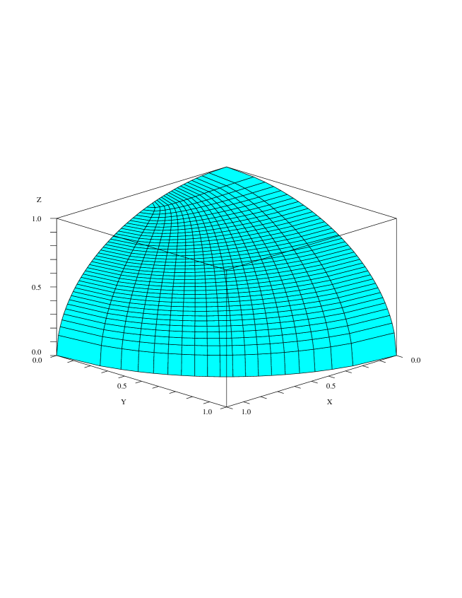
Figure 1: A uniform grid in the separating coordinates for $N=3$.

3 The Schrödinger equation.

We shall seek wave functions which factorize in the separating variables $t_{k}$:

$$\Psi(t_{1},\cdots,t_{N-1})=\Psi_{1}(t_{1})\,\Psi_{2}(t_{2})\cdots\Psi_{N-1}(t_{N-1})$$ (9)

the Hilbert space being the space of functions of variables $t_{i}$ with the measure:

$${\prod_{i>j}(t_{i}-t_{j})\over\sqrt{\prod_{i,k}|t_{i}-a_{k}|}}\prod_{i}dt_{i}$$

It has been shown in [7] that in order to simultaneously solve the eigenvalue equations $F_{k}\Psi=f_{k}\Psi$ all the $\Psi_{k}$ satisfy the same one–dimensional Schrödinger equation:

$$\left[{d^{2}\over dt^{2}}+{1\over 2}\sum_{k}{1\over t-a_{k}}\;{d\over dt}-{1\over 4\hbar^{2}}\sum_{k}{f_{k}\over t-a_{k}}\right]\,\Psi(t)=0$$ (10)

This is a linear differential equation with singularities at the $a_{k}$ and at infinity. More precisely at each $a_{k}$ there is a regular singularity [11], with exponents 0 and 1/2, while the singularity at infinity is irregular. Hence this equation appears as a generalization of the hypergeometric equation, however unlike the case of three regular singularities there doesn’t appear to exist integral formulae for the solution, precluding to perform explicit analytic continuation around the branch points at $a_{k}$.

There exists, fortunately, a workaround. Remark that all Hamiltonians $F_{k}$ are invariant under the $N$ parity transformations $(x_{j},y_{j})\to(-x_{j},-y_{j})$ so that one can simultaneously diagonalize both the Hamiltonians $F_{k}$ and the parities. That is, we can require that the wave function is even or odd in $x_{j}$ for each $j$, or equivalently that is is a function of the $x_{j}^{2}$ multiplied by a monomial $\prod x_{j}^{n_{j}}$ with $n_{j}\in\{0,1\}$. Let us now recall that if $t_{0}$ is a regular singularity with exponents $\alpha$, $\beta$, there exists convergent developments of the solution of the form

$$(t-t_{0})^{m}(p_{0}+p_{1}(t-t_{0})+p_{2}(t-t_{0})^{2}+\cdots)$$

where $m$ is $\alpha$ or $\beta$. The exponents being $0,\,1/2$ at each $a_{k}$, we see that these solutions are respectively even or odd under $x_{k}\to-x_{k}$, since $x_{k}\simeq\sqrt{t-a_{k}}$ for $t\to a_{k}$.

Moreover let us look at the parity properties of the wave function $\Psi$ in eq.(9) with respect to $x_{k}$. There are two ways to approach $x_{k}=0$:

$$t_{k}\to a_{k}~{}{\rm or}~{}t_{k-1}\to a_{k}\quad a_{k-1}<t_{k-1}<a_{k}<t_{k}<a_{k+1}$$

Requiring that the product $\Psi_{k-1}(t_{k-1})\Psi_{k}(t_{k})$ leads to a definite parity state in $x_{k}$ amounts to saying that $\Psi_{k-1}(t)$ and $\Psi_{k}(t)$ share the same exponent at $a_{k}$, hence both share the same analytic expansion in the interval $]a_{k-1},a_{k+1}[$. By induction, we arrive at the stronger statement that in order to have definite parities with respect to the $x_{k}$, all functions $\Psi_{k}$ in eq.(9) are in fact one and the same solution $\Psi(t)$ of the differential equation (10) on the whole interval $]a_{1},a_{N}[$, but constrained to have definite exponents at the points $a_{k}$, so as to produce the above monomial $\prod x_{j}^{n_{j}}$. This is the constraint which quantizes the $F_{k}$ in eq.(10). First it is clear that a wave function $\Psi$ so obtained on the quadrant $x_{k}\geq 0$ extends by parity to a univalued wave function on the sphere satisfying the Schrödinger equation. Second, start from a solution with definite exponent at $a_{1}$. In general its continuation to $a_{2}$ will be a superposition of the two pure exponent solutions. Requiring that there is no mixing imposes one condition on the $f_{k}$. Similarly at $a_{3},\ldots,a_{N}$ so that we get $N-1$ conditions on the $N-1$ independent $f_{k}$, the quantization conditions.

It remains to express these conditions in a form suitable for numerical analysis. We can always reduce the problem to the case where the solution is even under all $x_{k}\to-x_{k}$. Indeed if we want an odd solution, we have only to write $\Psi(t)=\sqrt{t-a_{k}}\Phi(t)$ and obtain the differential equation satisfied by $\Phi$, which is very similar to eq.(10). Then we require that $\Phi$ be even. Hence we need to express that the solution $\Psi(t)$ has a regular power series development at each point $a_{k}$. Inserting $\Psi(t)=p_{0}+p_{1}(t-t_{0})+p_{2}(t-t_{0})^{2}+\cdots$ in eq.(10) and requiring that the polar terms cancel we get the equation $p_{1}=p_{0}f_{k}/(2\hbar^{2})$, that is:

$$\Psi^{\prime}(a_{k})=\Psi(a_{k})f_{k}/(2\hbar^{2})$$ (11)

Of course these equations and eq.(10) are linear in $\Psi$ so a definite solution for $\Psi$ is obtained when requiring for example a normalization condition such as $\Psi(a_{1})=1$.

4 Numerical techniques.

The problem is now set in a form which happens to be directly tractable by a known numerical analysis package called COLNEW. This package allows to solve so–called mixed order boundary values problems: suppose we have a set of differential equations of various orders $u_{i}^{(m_{i})}=f_{i}(u)$ where $u$ is a vector of all functions $u_{i}$ and all their derivatives up to order $m_{i}-1$ for $u_{i}$, where $f$ may be linear or non linear. The general solution depends on $\sum m_{i}$ constants. The package allows to impose $\sum m_{i}$ “boundary conditions” and determines the solution satisfying all of them. These boundary conditions have to be of the form $g_{j}(u)(\zeta_{j})=0$ where $g_{j}$ are expressions of the same vector $u$ as above, and the points $\zeta_{j}$ are $\sum m_{i}$ points arbitrarily disposed in the considered domain or its boundary. The trick to apply this scheme to our problem is to treat the quantities $f_{k}$ as functions of $t$ which happen to be constant, i.e. satisfy $f_{k}^{\prime}=0$. Supplementing eq.(10) by these $N-1$ independent conditions we get a mixed order non linear differential system with total order $2+(N-1).1=N+1$. The boundary conditions we impose are the $N$ above equations $\Psi^{\prime}(a_{k})=\Psi(a_{k})f_{k}/(2\hbar^{2})$ at each $a_{k}$ plus a normalization such as $\Psi(a_{1})=1$ which completely fixes things.

Finally to appreciate how the numerical package can deal with the singularities at the $a_{k}$ appearing in eq.(10), it is in order to say a few words about it. The computation starts by cutting the considered interval into a number of subintervals. One is free to require that the $a_{k}$ are included in the subdivision. In each interval, the solution is approximated by some polynomial. The coefficients of these polynomials are fixed by a set of equations: first one requires that the differential equation is exactly satisfied at a number of so–called “collocation points” inside the intervals. These points are chosen at Gaussian positions as in numerical integration, in order to improve convergence. Note that, these points being interior while the $a_{k}$ are boundary points, we are always away from the poles in $1/(t-a_{k})$ when computing these equations. Second the package imposes that the solutions from interval to interval fit in a smooth way, and that the boundary conditions are obeyed. These conditions don’t suffer from divergent factors at $a_{k}$ and moreover imply in a finite way that the differential equation is indeed obeyed at the $a_{k}$ and that the solution has the appropriate parity property.

Things are set up so that one gets a non linear system for the coefficients, with as many equations as unknowns. This system is then solved by Newton–Raphson method, an error is evaluated, and a more refined solution is computed until a defined tolerance is obtained on all the equations. In practice we have found that the package works remarkably well for our problem, and is able to compute a fair number of solutions in a couple of seconds on a modern machine. Moreover its use is enhanced by the existence of a wrapper in Scilab which allows to program these computations in a convenient way.

The numerical results below will be restricted to the case $N=3$. There would not be any difficulty to study similarly higher dimensional problems. To reduce the parameter space to explore, we first normalize coefficients. Translating all the $a_{k}$ by the same quantity does not change the $F_{k}$ and adds a constant to the energy. We therefore set $a_{1}=0$. The equation (10) is also invariant by a common rescaling of $t$ and the $a_{k}$ by $\lambda$ and the rescaling of the $f_{k}$ by $1/\lambda$. The $\hbar$ factor can also be absorbed in the $f_{k}$ so that we are reduced to two parameters. We choose $a_{2}=1$ and have a parameter $y=a_{3}/a_{2}$ characterizing the asymmetry of the model. Now $\sum_{k}f_{k}=v$, where

$$v={a_{2}r^{2}\over 4\hbar^{2}},\quad r^{2}=\sum_{k}x_{k}^{2}$$ (12)

This single parameter can either be seen as characterizing the strength of the potential energy compared to the kinetic energy, or the approach to the semiclassical regime, which are therefore equivalent in this case. Finally, let us write the equations to be solved:

$$\hskip-28.45274pt\biggl{(}{d^{2}\over dt^{2}}+{1\over 2}\Bigl{(}{1\over t}+{1\over t-1}+{1\over t-y}\Bigr{)}{d\over dt}-$$

$$\hskip 28.45274pt\Bigl{(}{v-f_{2}-f_{3}\over t}+{f_{2}\over t-1}+{f_{3}\over t-y}\Bigr{)}\biggr{)}\Psi(t)=0$$ (13)

$$\hskip-28.45274pt\biggl{(}{d^{2}\over dt^{2}}+{1\over 2}\Bigl{(}{3\over t}+{1\over t-1}+{1\over t-y}\Bigr{)}{d\over dt}-$$

$$\hskip-14.22636pt\Bigl{(}{v-f_{2}-f_{3}+1/4+1/(4y)\over t}+{f_{2}-1/4\over t-1}+{f_{3}-1/(4y)\over t-y}\Bigr{)}\biggr{)}\Psi(t)=0$$ (14)

The second equation is the one we obtain when setting $\Psi\to\sqrt{t}\Psi$. There exist six similar equations describing, with the two displayed, the eight possible combinations of parities of the solution. Equation (13) is known as Wangerin’s equation, but its properties have not been explored. When $v=0$ the singularity at infinity becomes regular, and the equation reduces to Lamé’s equation. A great deal of work on this equation is summarized in [11], and is relevant for our study as we see below.

5 Numerical results.

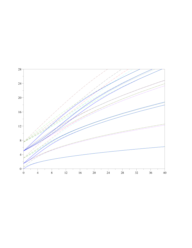
Figure 2: Energy as a function of $v$. Case $y=1.1$.

A single spectrum is not really instructive. We shall therefore show the evolution of the 36 lowest energy levels when the parameter $v$ grows. The number of different energy levels displayed is limited for the readability of the plots. States are characterized by their sets of parities and by the number of zeros of the wave function in each of the two intervals $]0,1[$ and $]1,y[$. The principal difficulty is to be able to choose a particular solution with a given number of zeros. The COLNEW package allows for a powerful mean to achieve this: an initial guess of the solution can be provided. However good guesses are not easy to find except for $v=0$. In this case, the theory of the Lamé spheroidal harmonics teaches us that the solutions which are analytic at the $a_{k}$ are polynomials. The zeros of these polynomials satisfy simple equations and it is therefore not difficult to give numerical approximations of the solutions. To reach higher values of $v$, we have used the continuation method, which consists in taking the solution for the old value of $v$ as the initial guess for the next value of $v$. If the difference between successive values of $v$ is sufficiently small, the new solution has the same quantum numbers. Below we have plotted $E/2=f_{2}+yf_{3}$ but we could have plotted individually each $f_{k}$ as a function of $v$.

To have an idea of the effect of the asymmetry parameter $y$, we plot the energies for three values of this parameter. The line styles correspond to the parity properties of the states. The heavy solid lines correspond to the states which are completely even, the other lines are solid or dashed according to the total parity of the states. In Fig. 2, $y$ is equal to 1.1, meaning that the two coordinates $x_{2}$ and $x_{3}$ are nearly equivalent. In fact, when $a_{k}=a_{k+1}$ there is a singular term in $F_{k}$ and $F_{k+1}$, but we can change for their sum and difference, with the sum being regular and the difference proportional to $J_{k,k+1}^{2}$. In this case of enhanced symmetry, the algebro–geometric solution of the classical model becomes singular, see [9], but the quantum solution has no particular trouble. Note however that a degeneracy of energy levels is apparent on the figure.

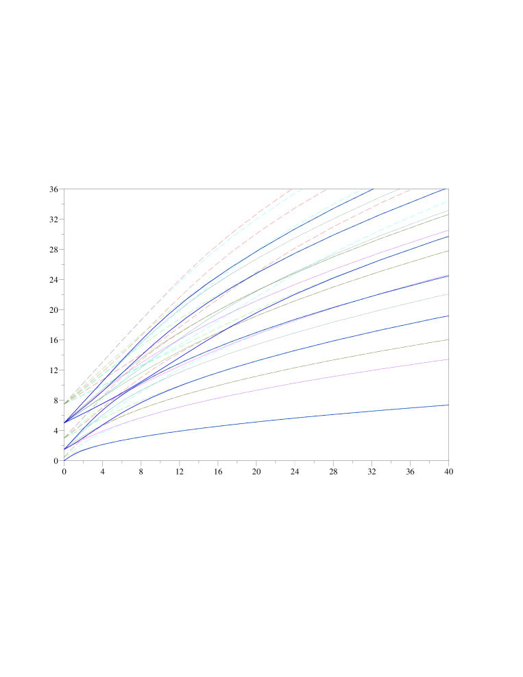
Figure 3: Energy as a function of $v$. Case $y=2$.

The case $y=2$ in Fig. 3 is representative of the case where the oscillator strengths are equally distributed, while the case $y=5$ in Fig. 4 illustrates the case where one of them is bigger. A remarkable feature of these plots is that the levels converge at $v=0$ to integer or half integer values. This is easily understood: $v=0$ is equivalent to setting the potential to zero, hence the problem has spherical symmetry, so the energy is equal to a factor times the eigenvalue of the $L^{2}$ operator, $j(j+1)$ with a $2j+1$ degeneracy. This is easily observed on the curves. An other feature of these plots is that pair of levels converge for large $v$. This can be understood from the potential barrier at the $x_{1}=0$ plane, so that the probability is concentrated around the opposite poles. In this limit, there are therefore two equivalent states, just separated by the exponentially small tunneling probability. When $v$ becomes even greater, the states occupy but a small patch around the poles and the effect of the curvature of the sphere becomes small. The problem reduces to the one of two independent harmonic oscillators, which have energies proportional to $\sqrt{v}$. Remark however that with growing quantum numbers, the level crossings between the two regimes $v$ small and $v$ large occur at larger values of $v$, so that for a given value of $v$, the eigenfunctions of sufficient energies are perturbations of the spheroidal harmonics.

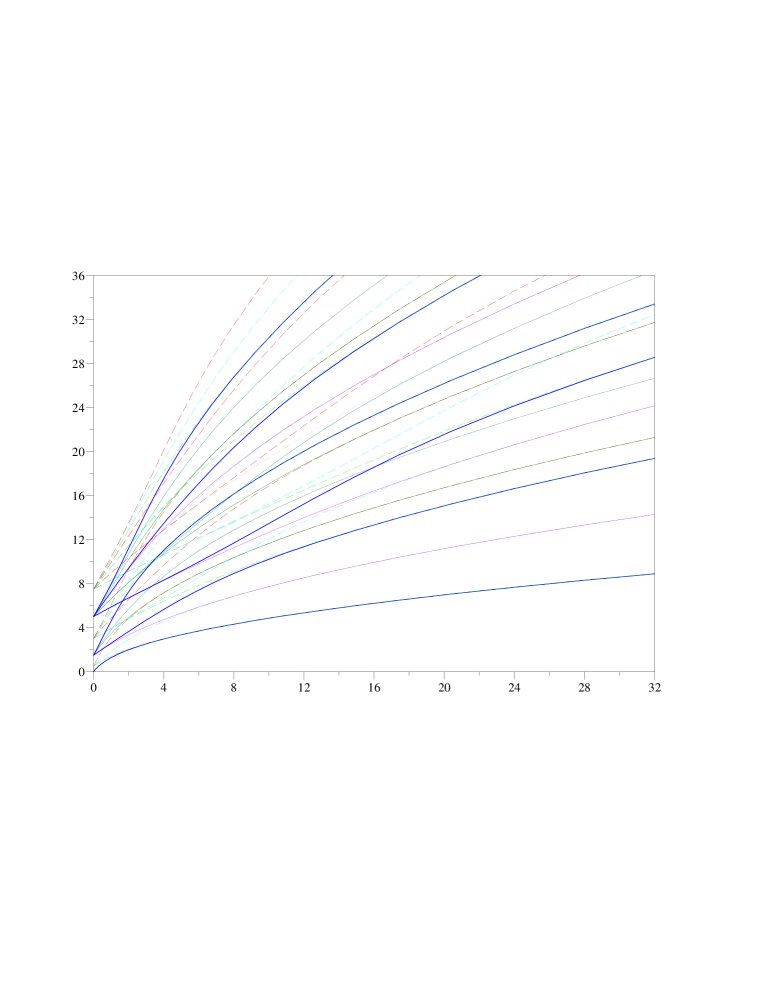
Figure 4: Energy as a function of $v$. Case $y=5$.

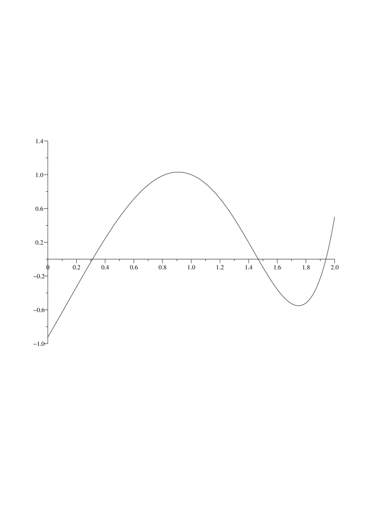
Figure 5: Eigenfunction. Case $y=2$ and $v=8$.

Finally the solution of eq. (10) for an excited state with $v=2$ and $y=2$ is plotted in figure (5). Precisely for this solution, which has one zero in $]0,1[$ and two zeroes in $]1,y[$ we have $f_{2}=-0.338$, $f_{3}=9.913$ hence the ”energy” is $f_{2}+yf_{3}=19.49$. Recall that the wave function is $\Psi(t_{1})\Psi(t_{2})$, with $0\leq t_{1}\leq 1\leq t_{2}\leq y$. Note that the locus of zeroes of the wave function is formed of intersecting lines due to the separation of variables. This is clearly non generic and would be destroyed by any perturbation. The existence of such singular node curves in the eigenstates of a quantum Hamiltonian is evidence for integrability.

6 Conclusion.

An efficient calculation of the spectrum of the quantum integrable Neumann model has been displayed. A number of degeneracies are evident from the above figures. It will be the purpose of a separate work to explicit these phenomena and relate them with the semiclassical analysis of the equation. This makes contact with the solution of the classical case in terms of hyperelliptic functions. The interesting features are the transitions between different semiclassical quantization conditions.

References

- [1] C. Neumann, De problemate quodam mechanico, quod ad primam integralium ultraellipticorum classem revocatur. Crelle Journal 56(1859), pp. 46–63.
- [2] J. Moser, Various aspects of integrable Hamiltonian systems. Proc. CIME bressanone, Progress in Mathematics, Birkhäuser (1978) 233.
- [3] K. Uhlenbeck, Minimal 2-spheres and tori in Sk. Preprint (1975).
- [4] D. Mumford. Tata lectures on Theta II. Birkhauser Boston, (1984).
- [5] J. Avan and M. Talon, Poisson structure and integrability of the Neumann-Moser-Uhlenbeck model. Intern. Journ. Mod. Phys. A 5 (1990), pp. 4477–4488.
- [6] O. Babelon and M. Talon, Riemann surfaces, separation of variables and classical and quantum integrability. Phys. Lett. A 312 (2003), pp. 71–77.
- [7] O. Babelon and M. Talon, Separation of variables for the classical and quantum Neumann model. Nucl. Phys. B379 (1992), pp. 321–339.
- [8] D. Gurarie, Quantized Neumann problem, separable potentials on Sn and the Lamé equation. J. Math. Phys. 36 (1995), pp. 5355–5391.
- [9] D. Bernard, O. Babelon and M. Talon. Introduction to classical integrable systems. Cambridge University Press, (2003).
- [10] E.K. Sklyanin. The quantum Toda chain. In Non-linear equations in classical and quantum field theory. Springer Notes in Physics, vol.226, (1985).
- [11] E.T. Whittaker and G.N. Watson. A course of modern analysis. Cambridge University Press, (1902).