SPHALERONS IN THE SKYRME MODEL

Abstract

Numerical methods are used to compute sphaleron solutions of the Skyrme model. These solutions have topological charge zero and are axially symmetric, consisting of an axial charge $n$ Skyrmion and an axial charge $-n$ antiSkyrmion (with $n>1$), balanced in unstable equilibrium. The energy is slightly less than twice the energy of the axially symmetric charge $n$ Skyrmion. A similar configuration with $n=1$ does not produce a sphaleron solution, and this difference is explained by considering the interaction of asymptotic pion dipole fields. For sphaleron solutions with $n>4$ the positions of the Skyrmion and antiSkyrmion merge to form a circle, rather than isolated points, and there are some features in common with Hopf solitons of the Skyrme-Faddeev model.

1 Introduction

Sphalerons are unstable classical solutions of field theories whose existence is due to non-trivial topological properties of the space of field configurations. Taubes was the pioneer of a topological approach to finding saddle point solutions and used this method to prove the existence of a monopole-antimonopole solution of the Yang-Mills-Higgs equations [27]. Subsequently, Manton used a similar approach to suggest the existence of an unstable solution in the Weinberg-Salam theory [20], which was then studied numerically in ref.[17] where the name sphaleron was coined. These, and other, successes prompted the search for a sphaleron in the Skyrme model, corresponding to a Skyrmion-antiSkyrmion solution in analogy with the monopole-antimonopole solution of the Yang-Mills-Higgs theory. However, despite the fact that the topological aspects are similar in the two theories, the current evidence [3, 12, 7] suggests that such a sphaleron is unlikely to exist, although it remains an open problem.

In this paper we observe that the asymptotic pion dipole interactions between Skyrmions and antiSkyrmions suggests that a more promising candidate for a saddle point solution consists of an axially symmetric charge $n$ Skyrmion balanced in unstable equilibrium with a charge $-n$ antiSkyrmion, where $n>1$ rather than $n=1.$ Note that for $n>2$ the constituents are themselves already saddle point solutions, since the minimal energy charge $n$ Skyrmion is not axially symmetric for $n>2$ [5].

Using numerical simulations of the Skyrme model we investigate this possibility and indeed are able to compute static saddle point solutions. Examples with $2\leq n\leq 6$ are presented in detail. They are axially symmetric and the energy is slightly less than twice the energy of the axial charge $n$ Skyrmion. Some comments on the topology associated with these solutions are made.

For $n=3$ and $n=4$ the solutions are qualitatively similar to the $n=2$ solution, with the separation between the Skyrmion and antiSkyrmion being smaller for larger values of $n.$ For $n>4$ the positions of the Skyrmion and antiSkyrmion are no longer isolated, but merge to form a circle, producing solutions which have some features in common with Hopf solitons of the Skyrme-Faddeev model [6, 8, 4, 9].

2 Topology and Interaction Energies

Let us begin by recalling the salient features behind the existence of Taubes’ monopole-antimonopole solution. Morse theory relates the topology of a manifold to the number and types of critical points of a function defined on the manifold. Taubes [27] was able to apply an infinite dimensional version of Morse theory, with the space of field configurations and the energy functional playing the role of the manifold and the function respectively. Topology enters through the non-triviality of certain homotopy groups, as follows. The space ${\cal C}^{\mbox{mon}}$ of finite energy Yang-Mills-Higgs field configurations (after suitably removing the gauge freedom) is homotopic to the space of maps from $S^{2}$ to $S^{2},$ which may be thought of as the space of Higgs fields at infinity. The degree of this map $N$ is the monopole number and this labels the connected components of ${\cal C}^{\mbox{mon}}$ since

$$\pi_{0}({\cal C}^{\mbox{mon}})=\pi_{0}(\mbox{Maps}(S^{2}\mapsto S^{2}))=\pi_{2}(S^{2})=\hbox{\mybb Z}.$$ (2.1)

The component ${\cal C}^{\mbox{mon}}_{0}$, with zero monopole number, has non-contractible loops since

$$\pi_{1}({\cal C}^{\mbox{mon}}_{0})=\pi_{1}(\mbox{Maps}(S^{2}\mapsto S^{2}))=\pi_{3}(S^{2})=\hbox{\mybb Z}$$ (2.2)

where now the maps between two-spheres must be restricted to those with degree zero.

A generator for this homotopy group is the non-contractible loop in configuration space in which a monopole-antimonopole pair is created from the vacuum, the pair are separated and the monopole rotated by $2\pi$ before the pair are brought together again to annihilate back to the vacuum. For any loop $\gamma$ in the same homotopy class as this one we can determine the maximal value $E_{\gamma}$ of the energy along this loop. Minimizing this maximal value over all loops $\gamma$ yields an unstable stationary point of the energy functional and this is the sphaleron. It is the midpoint of the non-contractible loop where the monopole is rotated by $\pi$ and the pair relax to the optimal separation to minimize the energy with this relative rotation. The pair can not relax to annihilate because the loop is non-contractible and hence the only other way that this procedure could fail to yield a sphaleron is if the relaxation produced a monopole-antimonopole pair with infinite separation. Taubes was able to rigorously rule out this possibility, and physically it corresponds to the fact that at large separation the interaction energy of a monopole-antimonopole pair is dominated by the Coulomb force which has a magnetic and (in the BPS limit) a scalar contribution which are both strictly attractive. This attraction at large separation therefore prevents the relaxation from producing a pair with infinite separation. The monopole-antimonopole solution is axially symmetric and has been computed numerically [23, 14], where its energy (in the BPS limit) is found to be $1.70$ times the energy of a single monopole.

Some aspects of the above analysis can be mirrored in the Skyrme model, though others can not, as we now briefly describe.

The space ${\cal C}^{\mbox{sky}}$ of finite energy Skyrme fields [24] is homotopic to the space of maps from $S^{3}$ to $S^{3}.$ The degree of the map $B$ is the baryon number and this labels the connected components of ${\cal C}^{\mbox{sky}}$ since

$$\pi_{0}({\cal C}^{\mbox{sky}})=\pi_{0}(\mbox{Maps}(S^{3}\mapsto S^{3}))=\pi_{3}(S^{3})=\hbox{\mybb Z}.$$ (2.3)

As for monopoles, the component ${\cal C}^{\mbox{sky}}_{0}$, with zero charge, has non-contractible loops since

$$\pi_{1}({\cal C}^{\mbox{sky}}_{0})=\pi_{1}(\mbox{Maps}(S^{3}\mapsto S^{3}))=\pi_{4}(S^{3})=\hbox{\mybb Z}_{2}$$ (2.4)

where we restrict to degree zero maps between three-spheres. Note that this result shows that in the Skyrme model there is only one type of non-contractible loop, compared to the infinite number for monopoles.

The non-contractible loop is generated by creating a Skyrmion-antiSkyrmion pair, separating them, rotating the Skyrmion by $2\pi$ and bringing the pair back together to annihilate. So far the discussion is very close to that for monopoles, the only difference being that rotating the Skyrmion by $4\pi$ instead of $2\pi$ is a contractible loop in the Skyrme model, but this is not important for the possible existence of a sphaleron. However, recall that a sphaleron could fail to exist if the minimax procedure results in a Skyrmion-antiSkyrmion pair with infinite separation, and this is where the crucial difference lies. For monopoles this does not happen because a monopole-antimonopole pair attract at large separations for all relative phases, but this is not true for a Skyrmion-antiSkyrmion pair.

From far away a Skyrmion resembles a triplet of orthogonal pion dipoles. Let us denote the dipole strength by $4\pi C,$ where $C$ is a positive constant. The leading order contribution to the interaction energy of a well separated Skyrmion-antiSkyrmion pair is given by the dipole-dipole interaction term. Consider a Skyrmion-antiSkyrmion pair with separation $s$ and the Skyrmion rotated by a phase $\alpha$ relative to the antiSkyrmion, about the line joining them. To leading order the energy of the pair is [3, 12]

$$E=2E_{1}-\frac{4C^{2}}{3\pi s^{3}}(1+\cos\alpha)$$ (2.5)

where $E_{1}$ denotes the energy of a single Skyrmion.

Providing the relative phase is not equal to $\pi$ then the interaction energy is negative so the Skyrmion and antiSkyrmion attract. However, if the phase is $\pi$ then the dipole-dipole interaction vanishes and a higher order calculation must be performed to determine the nature of the interaction. The result of such a calculation [12] reveals that the leading contribution to the interaction energy is of order $1/s^{6}$ and is positive, so that a Skyrmion and antiSkyrmion are repulsive when the relative phase is $\pi.$ The result of the minimax procedure is therefore a Skyrmion and antiSkyrmion with infinite separation, not a sphaleron. The numerical results presented in the following sections agree with this analysis and support the conclusion that there is no sphaleron in the Skyrme model that may be thought of as a single Skyrmion-antiSkyrmion pair.

Let us turn our attention, for the moment, to the minimal energy charge 2 Skyrmion. This is axially symmetric and its asymptotic fields resemble a single pion dipole aligned with the symmetry axis and with a dipole strength of approximately $8\pi C.$ This is because the charge 2 Skyrmion is formed by bringing together two single Skyrmions where one is rotated by $\pi$ around an axis (which will become the axis of symmetry) orthogonal to the line joining the two Skyrmions. The dipole fields which point along the axis will add whereas the others will cancel in pairs.

Now consider a well separated charge 2 Skyrmion and a charge $-2$ antiSkyrmion with a common axis of symmetry and separation $s.$ If the Skyrmion is rotated by a phase $\alpha$ about the symmetry axis then, because all the dipole fields lie along this axis, the leading order interaction energy will be negative and independent of $\alpha.$ To order $1/s^{3}$ the energy is given by

$$E=2E_{2}-\frac{16C^{2}}{3\pi s^{3}}$$ (2.6)

where $E_{2}$ is the energy of the charge 2 Skyrmion.

From the point of view of the interaction energy the charge 2 Skyrmion and charge $-2$ antiSkyrmion pair is qualitatively similar to the monopole-antimonopole pair. The leading order contribution to the interaction is attractive and independent of the phase, so the pair will not drift away to infinite separation. This configuration therefore has more chance of forming a sphaleron than the charge 1 Skyrmion and charge $-1$ antiSkyrmion pair, when only this aspect is considered.

As we discuss in detail in the appendix, there are good reasons to believe that for all $n>1$ the axially symmetric charge $n$ Skyrmion has asymptotic fields that consist of only a single pion dipole, which is aligned with the symmetry axis, and whose dipole strength increases with $n.$ Therefore the previous discussion of the nature of the interaction energy of a charge 2 Skyrmion and a charge $-2$ antiSkyrmion applies equally well to a configuration consisting of an axially symmetric charge $n$ Skyrmion and a charge $-n$ antiSkyrmion for all $n>1.$

Having seen that the dipole interaction between an axial charge $n$ Skyrmion and a charge $-n$ antiSkyrmion is favourable for the formation of a sphaleron let us now consider the topology of such a configuration.

The fields of the axially symmetric charge $n$ Skyrmion are invariant under a rotation by $2\pi/n$ around the symmetry axis. Note that although the Skyrmion is said to have an axial symmetry, generically a rotation by $\alpha$ around the axis of symmetry will change the fields, and axial symmetry refers to the fact that this change is equivalent to an isospin rotation by $\alpha n.$

The closed loop that is relevant for an axial charge $n$ Skyrmion and charge $-n$ antiSkyrmion pair is the creation of the pair from the vacuum, their separation, the rotation of the Skyrmion by $2\pi/n,$ and their subsequent annihilation. The hope is then that a sphaleron would be associated with the midpoint of this loop where the relative phase is $\pi/n.$ The closed loop which corresponds to the rotation by $2\pi/n$ around the symmetry axis of an axially symmetric charge $n$ Skyrmion is non-contractible if and only if $n$ is odd [18]. Thus the loop relevant for the sphaleron is only non-contractible if $n$ is odd. It therefore appears that the lowest value for which the interaction energy and topology combine to produce a sphaleron should be $n=3.$

Naively, there seems no reason to suppose a sphaleron should exist with $n=2$ (or any other even value) since the topology appears to be lost, but as we shall see it turns out that this conclusion is too hasty. It may be that the energy barrier provided by the non-zero relative phase is sufficient to yield a solution, or that the topology is more subtle. For example, it may be the existence of non-trivial higher homotopy groups that underlies the existence of these solutions. This is certainly a possibility in the Skyrme model as there are non-contractible spheres since

$$\pi_{2}({\cal C}^{\mbox{sky}}_{0})=\pi_{2}(\mbox{Maps}(S^{3}\mapsto S^{3}))=\pi_{5}(S^{3})=\hbox{\mybb Z}_{2}.$$ (2.7)

Another possibility is that although for even $n$ the loop is contractible in the full space of Skyrme fields it may not be contractible within the restricted space of axially symmetric Skyrme fields. It would be interesting to clarify this, but we have as yet been unable to do so. Should it be true then symmetry considerations prevent an axially symmetric field from breaking this symmetry during relaxation, so it should be sufficient to yield a sphaleron.

In this section we have made some arguments for the possible existence of sphalerons consisting of a charge $n$ Skyrmion and charge $-n$ antiSkyrmion, where $n>1.$ In the following sections we investigate this using numerical methods and find that indeed such solutions exist.

3 Axial Skyrmions

The static energy of the Skyrme model is given by

$$E=\frac{1}{12\pi^{2}}\int\left\{-{1\over 2}\mbox{Tr}(R_{i}R_{i})-{1\over 16}\mbox{Tr}([R_{i},R_{j}][R_{i},R_{j}])\right\}\,d^{3}x\,,$$ (3.1)

where $R_{i}=(\partial_{i}U)U^{\dagger}$ is the $su(2)$-valued current associated with the $SU(2)$-valued Skyrme field $U({\bf x}).$ With this normalization the Faddeev-Bogomolny bound is $E\geq|B|$ where the baryon number $B$ is

$$B=-{1\over 24\pi^{2}}\int\epsilon_{ijk}{\rm Tr}\left(R_{i}R_{j}R_{k}\right)\,d^{3}x.$$ (3.2)

To make contact with the nonlinear pion theory $U$ is written as

$$U=\sigma+i\mbox{\boldmath$\pi$}\cdot\mbox{\boldmath$\tau$}$$ (3.3)

where $\tau$ denotes the triplet of Pauli matrices, $\mbox{\boldmath$\pi$}=(\pi_{1},\pi_{2},\pi_{3})$ is the triplet of pion fields and $\sigma$ is determined by the constraint $\sigma^{2}+\mbox{\boldmath$\pi$}\cdot\mbox{\boldmath$\pi$}=1.$

In this paper we are only concerned with axially symmetric fields so we introduce the ansatz

$$\sigma=\psi_{3},\quad\pi_{1}=\psi_{1}\cos n\theta,\quad\pi_{2}=\psi_{1}\sin n\theta,\quad\pi_{3}=\psi_{2}$$ (3.4)

where $\mbox{\boldmath$\psi$}(\rho,z)=(\psi_{1},\psi_{2},\psi_{3})$ is a three-component unit vector which is a function only of $\rho$ and $z,$ where $\rho$ and $\theta$ are polar coordinates in the $(x_{1},x_{2})$ plane and $z=x_{3}.$ In the above ansatz $n$ is an integer that counts the planar winding of the fields.

Substituting the ansatz (3.4) into the Skyrme energy (3.1) gives

$$E=\frac{1}{6\pi}\int\{(\partial_{\rho}\mbox{\boldmath$\psi$}\cdot\partial_{\rho}\mbox{\boldmath$\psi$}+\partial_{z}\mbox{\boldmath$\psi$}\cdot\partial_{z}\mbox{\boldmath$\psi$})(1+\frac{n^{2}}{\rho^{2}}\psi_{1}^{2})+|\partial_{\rho}\mbox{\boldmath$\psi$}\times\partial_{z}\mbox{\boldmath$\psi$}|^{2}+\frac{n^{2}}{\rho^{2}}\psi_{1}^{2}\}\ \rho\,d\rho\,dz$$ (3.5)

which is a kind of Baby Skyrme model on the half-plane. The baryon number is given by

$$B=\frac{n}{\pi}\int\{\psi_{1}\mbox{\boldmath$\psi$}\cdot\partial_{\rho}\mbox{\boldmath$\psi$}\times\partial_{z}\mbox{\boldmath$\psi$}\}\ d\rho\,dz.$$ (3.6)

The finite energy boundary conditions are that $\mbox{\boldmath$\psi$}\rightarrow(0,0,1)$ as $\rho^{2}+z^{2}\rightarrow\infty,$ and on the symmetry axis $\rho=0$ we require $\psi_{1}=0$ and $\partial_{\rho}\psi_{2}=\partial_{\rho}\psi_{3}=0.$

A configuration with the correct topology and boundary conditions of an axially symmetric Skyrme field with $B=n$ is given by

$$\psi_{1}=\frac{\rho}{r}\sin f,\quad\psi_{2}=\frac{z}{r}\sin f,\quad\psi_{3}=\cos f$$ (3.7)

where $r=\sqrt{\rho^{2}+z^{2}}$ and $f(r)$ is a monotonically decreasing profile function with $f(0)=\pi$ and $f(\infty)=0.$

In order to create initial conditions for a charge $n$ Skyrmion and a charge $-n$ antiSkyrmion pair (which of course has total charge $B=0$) with separation $s$ we perform the following construction. Let $\mbox{\boldmath$\psi$}^{(1)}$ be a configuration of the form (3.7) with profile function $f(r)=\pi(1-2r/s)$ for $r\leq s/2$ and zero otherwise. Now make the replacement $z\mapsto z-s/2$ so that the charge $n$ Skyrmion is located at $z=s/2$ on the symmetry axis. Let $\mbox{\boldmath$\psi$}^{(2)}$ be a similar configuration but this time shifted by $z\mapsto z+s/2$ so that it is located at $z=-s/2.$ To turn this second Skyrmion into an antiSkyrmion we make the reflection

$$(\psi^{(2)}_{1},\psi^{(2)}_{2},\psi^{(2)}_{3})\mapsto(\psi^{(2)}_{1},-\psi^{(2)}_{2},\psi^{(2)}_{3})$$ (3.8)

which we refer to as an antiSkyrmion with zero relative phase, compared to the original Skyrmion. Note that this reflection changes the sign of only one of the pion fields and so our definition of the relative phase differs by an addition of $\pi$ in comparison with that of refs.[3, 12, 7], where the antiSkyrmion is obtained by changing the sign of all three of the pion fields. However, the definition used in this paper makes for a more natural comparison with the similar situation for monopoles.

The fields of a charge $n$ Skyrmion are invariant under a rotation around the symmetry axis by $2\pi/n,$ so the midpoint of the loop we are interested in corresponds to a rotation by $\pi/n.$ From (3.4) we see that the rotation $\theta\mapsto\theta+\pi/n$ changes the sign of the pion fields $\pi_{1}$ and $\pi_{2}$ and so is equivalent to the change $\psi_{1}\mapsto-\psi_{1}.$ Thus to obtain a charge $n$ antiSkyrmion which is out of phase with the charge $n$ Skyrmion (in the sense of being at the midpoint of the loop) we replace the transformation (3.8) with

$$(\psi^{(2)}_{1},\psi^{(2)}_{2},\psi^{(2)}_{3})\mapsto(-\psi^{(2)}_{1},-\psi^{(2)}_{2},\psi^{(2)}_{3}).$$ (3.9)

Finally, the fields are defined to be

$$\mbox{\boldmath$\psi$}=\cases{\mbox{\boldmath$\psi$}^{(1)}\quad\mbox{ if}\quad\sqrt{(z-s/2)^{2}+\rho^{2}}\leq s/2\cr\mbox{\boldmath$\psi$}^{(2)}\quad\mbox{ if}\quad\sqrt{(z+s/2)^{2}+\rho^{2}}\leq s/2\cr(0,0,1)\quad\quad\mbox{otherwise.}}$$ (3.10)

The profile function is zero at a radius $s/2$ from the centre of the Skyrmion (or antiSkyrmion), so the Skyrmion and antiSkyrmion are patched together in a continuous way, with the fields set to the vacuum outside each of the cores. This method of creating initial conditions is preferable to using a product ansatz with a minimal energy profile function, since the product ansatz does not respect the symmetries of the configuration in the same way that the patching ansatz (3.10) does.

In the following section we discuss the results of a numerical relaxation of axially symmetric Skyrmion-antiSkyrmion pairs using the initial conditions described above. In addition to the initial conditions using the simple ansatz (3.7), more sophisticated initial conditions were also used based on the rational map ansatz [11] with an axially symmetric charge $n$ map. Either ansatz leads to the same final solutions, though the rational map ansatz relaxes slightly faster since it provides a better approximation to the axial charge $n$ Skyrmion.

4 Numerical Results

To find stationary points of the energy (3.5) we solve the associated gradient flow equation. This is an evolution equation which is first order in a fictitious time and where the velocity of the field is given by minus the variation of the energy, taking into account the unit vector constraint. We do not present the details of this equation here since it is rather cumbersome and not particularly enlightening. The end point of the gradient flow evolution is then the required stationary point of the energy. The gradient flow equation is solved numerically using a finite difference scheme which is second order accurate in the spatial derivatives and first order in the time derivatives. The grid in the $(\rho,z)$-plane contains $200\times 400$ points with a lattice spacing of $0.05$ so that the range covered is $(\rho,z)\in[0,10]\times[-10,10].$

Figure 1: The separation $s$ and energy $E$ (in units of the energy of a single Skyrmion) as a function of time, for a charge 1 Skyrmion and charge $-1$ antiSkyrmion pair with a relative phase of $\pi.$

Figure 2: The separation $s$ and energy $E$ (in units of $E_{2}$) as a function of time, for a charge 2 Skyrmion and charge $-2$ antiSkyrmion pair with zero relative phase.

As a test on the numerical code we first perform two simulations which are not expected to lead to a sphaleron solution. The first simulation consists of a charge 1 Skyrmion and charge $-1$ antiSkyrmion pair with a relative phase of $\pi.$ The initial conditions are created using the ansatz described in the previous section with an initial separation $s=2.$ In Fig. 1 we plot the separation $s,$ and the energy $E$ divided by the energy of a single Skyrmion ($E_{1}=1.232$), as a function of time during the gradient flow evolution. The separation is computed from the positions of the Skyrmion and antiSkyrmion, which are defined to be the points in space where the $\sigma$ field is equal to $-1.$ The separation increases with time and the energy tends towards twice the energy of a single Skyrmion, confirming the repulsive force between this pair.

For the second simulation we turn to the charge 2 Skyrmion and charge $-2$ antiSkyrmion pair. Fig. 2 displays the results of an initial configuration with separation $s=4$ and zero relative phase. The separation rapidly decreases to zero, as does the energy, demonstrating that the pair annihilate. The energy is plotted in units of $E_{2},$ the energy of the axially symmetric charge 2 Skyrmion. In this paper $E_{n}$ denotes the energy of the axially symmetric charge $n$ Skyrmion, and energies will be plotted in these units for ease of comparison. The values used for $E_{n}$ can be found in the third column of Table 1 and were computed using the same code with the same lattice values, so that an accurate computation of the relative energies should result.

Figure 3: The separation $s$ and energy $E$ (in units of $E_{2}$) as a function of time, for a charge 2 Skyrmion and charge $-2$ antiSkyrmion pair with relative phase $\pi/2.$

Fig. 3 displays the results for a charge 2 Skyrmion and charge $-2$ antiSkyrmion pair again with an initial separation $s=4$ but this time with a relative phase of $\pi/2.$ As expected from the dipole analysis, the separation initially decreases but it then tends to an asymptotic value $s=2.89,$ at which the energy is $1.967$ times the energy of the axially symmetric charge 2 Skyrmion ie. the energy is slightly less than the energy of the Skyrmion-antiSkyrmion constituents. This is the sphaleron solution. The sphaleron energy density in the $(z,\rho)$-plane is displayed in Fig. 4.

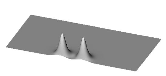
Figure 4: The sphaleron energy density in the $(z,\rho)$-plane.

Figure 5: The $\sigma$ field along the $z$-axis for the sphaleron solution formed from the charge $n$ Skyrmion and charge $-n$ antiSkyrmion, where $n=2$ (solid curve), $n=3$ (dashed curve), $n=4$ (dotted curve).

The charge 2 Skyrmion and charge $-2$ antiSkyrmion are clearly visible as distinct structures and this explains why the energy is only very slightly less than twice the energy of the charge 2 Skyrmion. The $\sigma$ field along the $z$-axis is plotted as the solid curve in Fig. 5, where the soliton positions ($\sigma=-1$) can be seen on the $z$-axis at $z=\pm 1.445.$ Note that between the pair the field is far from the vacuum value $\sigma=1.$

$n$	$E$	$E_{n}$	$E/E_{n}$	$(z,\rho)$
2	4.645	2.362	1.967	$(\pm 1.445,0)$
3	6.947	3.581	1.940	$(\pm 1.096,0)$
4	9.323	4.863	1.917	$(\pm 0.653,0)$
5	11.656	6.141	1.898	$(0,1.303)$
6	14.054	7.481	1.879	$(0,2.082)$

Table 1: For $2\leq n\leq 6$ the table shows the energy $E$ of the sphaleron consisting of a charge $n$ Skyrmion and a charge $-n$ antiSkyrmion pair, the energy $E_{n}$ of the axially symmetric charge $n$ Skyrmion, the ratio $E/E_{n},$ and the position of the Skyrmion and antiSkyrmion in the $(z,\rho)$-plane.

Higher energy sphaleron solutions are formed from a charge $n$ Skyrmion and charge $-n$ antiSkyrmion pair with a relative phase of $\pi/n,$ where $n>2.$ For $n=3$ and $n=4$ the sphaleron solution is qualitatively similar to the case of $n=2.$ Table 1 lists the energies of these sphalerons, a comparison with the energies of axial charge $n$ Skyrmions, and the positions of the Skyrmion-antiSkyrmion pair in the $(z,\rho)$-plane. In Fig. 5 the $\sigma$ field along the $z$-axis is plotted as the dashed curve for $n=3$ and the dotted curve for $n=4.$ Table 1 and Fig. 5 demonstrate that the charge $n$ Skyrmion and charge $-n$ antiSkyrmion pair sit closer together and are more tightly bound as $n$ increases. This is consistent with the fact that the dipole strength of the axial charge $n$ Skyrmion increases with $n.$ Recall that, as discussed earlier, in the case $n=3$ the sphaleron is associated with a non-contractible loop, since the relevant loop is non-contractible when $n$ is odd. Thus it might be possible to rigorously prove the existence of this $n=3$ sphaleron solution using Taubes’ approach.

For $n>4$ the sphaleron solution has an interesting qualitative difference with the solutions described so far. The energies presented in Table 1 for $n=5$ and $n=6$ follow a similar trend to the $n=2,3,4$ solutions. However, an examination of the $\sigma$ field reveals that the positions of the Skyrmion and antiSkyrmion are no longer two isolated points on the $z$-axis, but merge to form a circle. Fig. 6 plots the $\sigma$ field along (a) the $z$-axis and (b) the $\rho$-axis, for $n=5$ (solid curves) and $n=6$ (dashed curves). It can be seen that the $\sigma$ field never attains the value $-1$ along the $z$-axis, and in fact the minimal value along this axis increases with $n.$ The $\sigma$ field is $-1$ on a circle in the $z=0$ plane of radius $\rho=1.303$ for $n=5$ and radius $\rho=2.082$ for $n=6.$ The Skyrmion and antiSkyrmion can no longer be identified, having merged so that they are both located on a whole circle. As we now describe, these solutions have some features in common with Hopf solitons of the Skyrme-Faddeev model.

Figure 6: The $\sigma$ field along (a) the $z$-axis and (b) the $\rho$-axis for the sphaleron solution formed from the charge $n$ Skyrmion and charge $-n$ antiSkyrmion, where $n=5$ (solid curves) and $n=6$ (dashed curves).

The field of the Skyrme-Faddeev model [6] is a three-component unit vector, and it has topological soliton solutions classified by the integer-valued Hopf invariant associated with the homotopy group $\pi_{3}(S^{2})=\hbox{\mybb Z}.$ Solutions of the Skyrme-Faddeev model automatically yield solutions of the Skyrme model by an embedding which sets one of the pion fields to zero (say $\pi_{3}$) and maps the unit vector onto the $\sigma$ field and the two remaining pion fields. Such embedded solutions have zero baryon number and are expected to be unstable, so they are sphaleron-like, but there is no obvious interpretation in terms of Skyrmion-antiSkyrmion pairs.

The lowest energy Hopf soliton with Hopf charge one has a Skyrme energy of about $4.4$ (in the units we are using) so it has less energy than any of the sphalerons presented in this paper. Axially symmetric Hopf solitons exist for all Hopf charges $Q,$ although for $Q>2$ they are not the minimal energy solitons and are unstable even within the Skyrme-Faddeev model [4]. Such axially symmetric solutions fit into the class described by the ansatz (3.4) with $\psi_{2}=0$ and $Q=n.$ The $\sigma$ field is $-1$ on a circle and the pion fields $\pi_{1},\pi_{2}$ rotate $n$ times around this circle, so these solutions are qualitatively similar to the sphaleron solutions formed from a charge $n$ Skyrmion and charge $-n$ antiSkyrmion provided $n>4.$ The energies [4] of the embedded axial Hopf solitons with $n=5$ and $n=6$ are $E=16.7$ and $E=19.9,$ so a comparison with Table 1 shows that it is not energetically favourable to set $\psi_{2}=0$ for these values of $n$.

We have seen that as $n$ increases the sphaleron solution has a $\sigma$ field along the $z$-axis whose deviation from the vacuum value diminishes. Embedded Hopf solitons have $\sigma=1$ along the entire $z$-axis, so it may be that the sphaleron and Hopf soliton solutions tend towards the same field configurations for large $n.$ It might be interesting to investigate this possibility in more detail in the future.

5 Conclusion

In this paper we have discussed how considerations of asymptotic pion dipole fields and topology combine to suggest the existence of sphaleron solutions in the Skyrme model. These sphalerons consist of an axial charge $n$ Skyrmion and an axial charge $-n$ antiSkyrmion (with $n>1$) balanced in unstable equilibrium. We have then used numerical methods to compute these solutions and have described their properties in some detail. The solutions appear to exists for all $n>1,$ but the topological aspects are better understood for odd $n$, and some open problems remain in clarifying the more subtle role of the topology for even $n,$ though we have made some suggestions for further investigation.

For $n>4$ a new interesting phenomenon occurs, with the position of the Skyrmion and antiSkyrmion merging to form a circle, rather than two isolated points. A similar phenomenon occurs in the Yang-Mills-Higgs model, where charge $n$ monopole and charge $-n$ antimonopole solutions also exist with $n\geq 1$ [22, 15], and for $n>2$ the Higgs field is zero on a circle. This is another example of the similarity that is often found between monopoles and Skyrmions. There are also monopole-antimonopole chains [16] where monopoles and antimonopoles alternate along a line, and we expect similar solutions to exist in the Skyrme model, provided the constituents are not single Skyrmions or single antiSkyrmions.

Although the physical implications of saddle point solutions in quantum field theory are not easily deduced, the existence of sphaleron solutions in the Skyrme model may have ramifications which can be investigated experimentally. The simplest sphaleron solution we have found is relevant to deuterium-antideuterium annihilation, and although experiments can not yet investigate this process, the recent experimental successes in studying antihydrogen [1] suggest it may be a possibility in the near future.

Finally, the results presented in this paper may have technological significance in future years, since apparently the engines of Star Trek starships are powered by deuterium-antideuterium reactors [25].

Appendix

In this appendix we discuss the asymptotic pion dipole fields of the axially symmetric charge $n$ Skyrmion, where $n>1.$

From numerical calculations it is difficult to determine the asymptotic fields of a Skyrmion which is not spherically symmetric, since a region is required which is both far from the Skyrmion core and far from the boundary of the grid, and this is difficult to achieve. Therefore, we present two approximate calculations which both suggest that for all $n>1$ the axially symmetric charge $n$ Skyrmion has asymptotic fields that consist of only a single pion dipole, which is aligned with the symmetry axis, and whose dipole strength increases with $n.$

Manton [21] has pointed out that it is often possible to predict the asymptotic multipole fields of a given Skyrmion by simply adding together the individual dipole fields of its constituents, if it is known how to arrange the individual Skyrmions so that the required Skyrmion will result.

As we have discussed earlier, the fields of the axially symmetric charge $n$ Skyrmion are strictly invariant under a rotation around the symmetry axis through an angle $2\pi/n.$ It is possible to arrange $n$ well separated single Skyrmions so that this cyclic subgroup is realized, and it is likely that this is the appropriate alignment to yield the axially symmetric charge $n$ Skyrmion. Similar cyclic arrangements of monopoles indeed lead to scattering processes which pass through the axially symmetric monopole [10, 26].

Generically, a Skyrmion has a dipole as its leading multipole

$$\pi_{j}=\frac{C_{ji}{\bf x}_{i}}{r^{3}}$$ (5.1)

where $4\pi C_{ji}$ is the dipole moment matrix. For a single Skyrmion we can choose the orientation so that

$$C_{ji}=\pmatrix{c&0&0\cr 0&c&0\cr 0&0&c}.$$ (5.2)

Arrange $n$ Skyrmions with positions

$${\bf X}^{(k)}=(L\cos\frac{2\pi k}{n},L\sin\frac{2\pi k}{n},0),\quad\quad k=1,\ldots,n$$ (5.3)

where $L$ is a separation scale. If the orientations of the pion fields are chosen to be

$$C^{(k)}=c\pmatrix{\cos({2\pi k}/{n})&-\sin({2\pi k}/{n})&0\cr\sin({2\pi k}/{n})&\cos({2\pi k}/{n})&0\cr 0&0&1\cr}$$ (5.4)

then this arrangement has cyclic symmetry, since under a spatial rotation by $2\pi/n$ around the $x_{3}$-axis, Skyrmion $k$ is rotated into Skyrmion $k+1$ and $C^{(k)}$ maps to $C^{(k+1)}.$

The sum of the dipole moment matrices gives

$$\sum_{k=1}^{n}C^{(k)}=\pmatrix{0&0&0\cr 0&0&0\cr 0&0&cn}$$ (5.5)

and so suggests that the axially symmetric Skyrmion has asymptotic fields that consist of only a single pion dipole, which is aligned with the symmetry axis, and whose dipole strength is proportional to $n.$ This argument is rather simple, and so the finer details should not be trusted too much, but it seems likely that the qualitative picture is correct, and for example the dipole field is likely to grow with $n,$ though a simple linear growth is probably too simplistic.

An approximate method for obtaining charge $n$ Skyrmions is through the holonomy of a four-dimensional charge $n$ Yang-Mills instanton [2]. For the axially symmetric Skyrmion the relevant instanton is of the JNR type [13] and is determined by a solution of the Laplace equation of the form

$$\zeta=\sum_{k=0}^{n}\frac{\lambda_{k}}{|x-a_{k}|^{2}}$$ (5.6)

where $x$ is the coordinate in four-dimensional Euclidean space, $\lambda_{k}=\frac{1}{n+1}$ are equal weights, and $a_{k\mu}=(L\cos\frac{2\pi k}{n+1},L\sin\frac{2\pi k}{n+1},0,0)$ are pole positions with $L$ a length scale.

Defining the quantity

$$Q_{\mu\nu}=\sum_{k=0}^{n}\lambda_{k}a_{k\mu}a_{k\nu}$$ (5.7)

then the asymptotic dipole fields of the instanton generated Skyrmion are given by [19]

$$\pi_{k}=-\frac{\pi}{2}(Q_{11}+Q_{22}+Q_{33}-Q_{44})\frac{x_{k}}{r^{3}}+(Q_{kj}-\varepsilon_{ijk}Q_{i4})\frac{\pi x_{j}}{r^{3}}.$$ (5.8)

Substituting the above values yields

$$\pi_{k}=-\frac{L^{2}\delta_{k3}\pi x_{3}}{2r^{3}}$$ (5.9)

which again suggests only a single pion dipole field aligned with the symmetry axis. Note that the sign is irrelevant here since there is only one non-zero component so its sign can be changed by an isospin transformation. The scale $L$ needs to be fixed in the instanton approximation by a minimization over $L$ of the energy of the resulting approximate Skyrmion. Since the size of an axially symmetric Skyrmion grows with $n$ it is expected that so does the minimizing scale $L,$ so again the prediction is that the dipole strength should increase with $n,$ in broad agreement with the prediction of the first approach.

References

- [1] M. Amoretti et al, Production and detection of cold antihydrogen atoms, Nature 456, 419 (2002).
- [2] M. F. Atiyah and N. S. Manton, Skyrmions from instantons, Phys. Lett. B222, 438 (1989); Geometry and kinematics of two Skyrmions, Commun. Math. Phys. 153, 391 (1993).
- [3] J. Bagger, W. Goldstein and M. Soldate, Static solutions in the vacuum sector of the Skyrme model, Phys. Rev. D31, 2600 (1985).
- [4] R. A. Battye and P. M. Sutcliffe, Knots as stable soliton solutions in a three-dimensional classical field theory, Phys. Rev. Lett. 81, 4798 (1998); Solitons, links and knots, Proc. R. Soc. Lond. A455, 4305 (1999).
- [5] R. A. Battye and P. M. Sutcliffe, Solitonic fullerene structures in light atomic nuclei, Phys. Rev. Lett. 86, 3989 (2001); Skyrmions, fullerenes and rational maps, Rev. Math. Phys. 14, 29 (2002).
- [6] L. Faddeev and A. J. Niemi, Stable knot-like structures in classical field theory, Nature 387, 58 (1997).
- [7] T. Gisiger and M. B. Paranjape, Recent mathematical developments in the Skyrme model, Phys. Reports 306, 109 (1998).
- [8] J. Gladikowski and M. Hellmund, Static solitons with nonzero Hopf number, Phys. Rev. D56, 5194 (1997).
- [9] J. Hietarinta and P. Salo, Faddeev-Hopf knots: dynamics of linked un-knots, Phys. Lett. B451, 60 (1999).
- [10] N. J. Hitchin, N. S. Manton and M. K. Murray, Symmetric monopoles, Nonlinearity 8, 661 (1995).
- [11] C. J. Houghton, N. S. Manton and P. M. Sutcliffe, Rational maps, monopoles and Skyrmions, Nucl. Phys. B510, 507 (1998).
- [12] K. Isler, J. LeTourneux and M. B. Paranjape, Morse theory and the Skyrmion-Skyrmion potential, Phys. Rev. D43, 1366 (1990).
- [13] R. Jackiw, C. Nohl and C. Rebbi, Conformal properties of pseudoparticle configurations, Phys. Rev. D15, 1642 (1977).
- [14] B. Kleihaus and J. Kunz, Monopole-antimonopole solution of the Yang-Mills-Higgs model, Phys. Rev. D61, 025003 (2000).
- [15] B. Kleihaus, J. Kunz and Ya. Shnir, Monopoles, antimonopoles and vortex rings, Phys. Rev. D68, 101701 (2003).
- [16] B. Kleihaus, J. Kunz and Ya. Shnir, Monopole-antimonopole chains, Phys. Lett. B570, 237 (2003).
- [17] F. R. Klinkhamer and N. S. Manton, A saddle-point solution in the Weinberg-Salam theory, Phys. Rev. D30, 2212 (1984).
- [18] S. Krusch, Homotopy of rational maps and the quantization of Skyrmions, Ann. Phys. 304, 103 (2003).
- [19] R. A. Leese and N. S. Manton, Stable instanton-generated Skyrme fields with baryon numbers three and four, Nucl. Phys. A572, 575 (1994).
- [20] N. S. Manton, Topology in the Weinberg-Salam theory, Phys. Rev. D28, 2019 (1983).
- [21] N. S. Manton, Skyrmions and their pion multipole moments, Acta Phys. Pol. B25, 1757 (1994).
- [22] V. Paturyan and D. H. Tchrakian, Monopole-antimonopole solution of the Skyrmed Yang-Mills-Higgs model, J. Math. Phys. 45, 302 (2004).
- [23] B. Rüber, Eine axialsymmetrische magnetische Dipollösung der Yang-Mills-Higgs-Gleichungen, Diplomarbeit, Universität Bonn, 1985.
- [24] T. H. R. Skyrme, A nonlinear field theory, Proc. R. Soc. Lond. A260, 127 (1961).
- [25] R. Sternback and M. Okuda, Star Trek: The next generation technical manual, Pocket Books (1991).
- [26] P. M. Sutcliffe, Cyclic monopoles, Nucl. Phys. B505, 517 (1997).
- [27] C. H. Taubes, The existence of a non-minimal solution to the Yang-Mills-Higgs equations on : Part I, Commun. Math. Phys. 86, 257 (1982); The existence of a non-minimal solution to the Yang-Mills-Higgs equations on : Part II, ibid 86, 299 (1982).