HU-EP-04-36

Generalizations of the AdS/CFT correspondence

Ingo Kirsch

Institut für Physik

Humboldt-Universität zu Berlin

Newtonstraße 15

D-12489 Berlin, Germany

Abstract

We consider generalizations of the AdS/CFT correspondence in which probe branes are embedded in gravity backgrounds dual to either conformal or confining gauge theories. These correspond to defect conformal field theories (dCFT) or QCD-like theories with fundamental matter, respectively. Moreover, starting from the dCFT we discuss the deconstruction of intersecting M5-branes and M-theory. We obtain the following results:

i) Holography of defect conformal field theories. We consider holography for a general D3-D$p$ brane intersection in type IIB string theory ($p\in\{3,5,7\}$). The corresponding near-horizon geometry is given by a probe AdS-brane in $AdS_{5}\times S^{5}$. The dual defect conformal field theory describes ${\cal N}=4$ super Yang-Mills degrees of freedom coupled to fundamental matter on a lower-dimensional space-time defect. We derive the spectrum of fluctuations about the brane embedding and determine the behaviour of correlation functions involving defect operators. We also study the dual conformal field theory in the case of intersecting D3-branes. To this end, we develop a convenient superspace approach in which both two- and four-dimensional fields are described in a two-dimensional $(2,2)$ superspace. We show that quantum corrections vanish to all orders in perturbation theory, such that the theory remains a (defect) conformal field theory when quantized.

ii) Flavour in generalized AdS/CFT dualities. We present a holographic non-perturbative description of QCD-like theories with a large number of colours by embedding D7-brane probes into two non-supersymmetric gravity backgrounds. Both backgrounds exhibit confinement of fundamental matter and a discrete glueball and meson spectrum. We numerically compute the $\bar{\psi}\psi$ quark condensate and meson spectrum associated with these backgrounds. In the first background, we find some numerical evidence for a first order phase transition at a critical quark mass where the D7 embedding undergoes a geometric transition. In the second, we find a chiral symmetry breaking condensate as well as the associated Goldstone boson.

iii) Deconstruction of extra dimensions. We apply the deconstruction method to the dCFT of intersecting D3-branes to obtain a field theory description for intersecting M5-branes. The resulting theory corresponds to two six-dimensional (2,0) superconformal field theories which we show to have tensionless strings on their four-dimensional intersection. Moreover, we argue that the $SU(2)_{L}$ R-symmetry of the dCFT matches the manifest $SU(2)$ R-symmetry of the M5-M5 intersection. We finally explore the fascinating idea of deconstructing M-theory itself. We give arguments for an equivalence of M-theory on a certain background with the Higgs branch of a four-dimensional non-supersymmetric (quiver) gauge theory: In addition to a string theoretical motivation, we find wrapped M2-branes in the mass spectrum of the quiver theory at low energies.

        And since the portions of the great and of the small are equal in amount, for this reason, too, all things will be in everything; nor is it possible for them to be apart, but all things have a portion of everything. Since it is impossible for there to be a least thing, they cannot be separated, nor come to be by themselves; but they must be now, just as they were in the beginning, all together. And in all things many things are contained, and an equal number both in the greater and in the smaller of the things that are separated off.

Anaxagoras of Clazomenae (500-428 B.C.)

1 Introduction

Holography is an ever fascinating concept since the early days of natural philosophy in ancient Greece. In modern language, holography (from the Greek word ‘holo’, meaning ‘whole’, and ‘graphy’, meaning ‘(the form of) writing’) means that all the physics in a volume of arbitrary dimension can be described in terms of the degrees of freedom of the surface or boundary of the volume with one less dimension. This definition is in analogy to a traditional hologram which stores a three-dimensional image in a two-dimensional surface. A philosophy which has a resemblance to holography is the ontology of Anaxagoras (500-428 B.C.). He was one of the pre-Socratics who wanted to solve the problem of change posed by Parmenides (504-456 B.C.). Anaxagoras suggested that each and every substance of the universe may be divided infinitely into ever smaller parts, but even in the tiniest part of the world there are fragments of all other things. His notion of “everything in everything” can most appropriately be illustrated by a hologram. Unlike normal photographs, every part of a hologram contains all the information possessed by the whole. In other words, if a hologram is fragmented, each piece of the hologram depicts a smaller version of the original picture and not just a part of it.

The philosophy of Anaxagoras fell behind due to the success of the “atomic theory” of Democritus (ca. 460-370 B.C.), another pre-Socratic philosopher. Democritus’ idea of an indivisible object (the a-tom) entered physics at the beginning of the 20th century when Rutherford and Bohr developed their atom models. Much later, these developments led to the concept of elementary particles which are nowadays described by the Standard Model of Elementary Particle Physics. The “Standard Model” is a term used to describe the quantum theory that includes the theory of strong interactions (quantum chromodynamics or QCD) and the unified theory of weak and electromagnetic interactions (electroweak). Though the Standard Model is substantially confirmed by experiment, it is incomplete in the sense that it does not incorporate gravity. To overcome this shortcoming, physicists seek for a unified theory which describes all forces including gravity. The most promising candidate is currently string theory which describes nature by tiny one-dimensional objects called “strings”.

String theory has its origin as an attempted theory of strong interactions [3, 4, 5] in 1970. However, in the years 1973 and 1974 an alternative theory of the strong interaction emerged in the form of quantum chromodynamics (QCD) replacing the previous string models (also called “dual resonance models”). It was then realised that dual models contain spin 2 particles with gravity-like couplings [6]. The original motivation for string theory as a theory of hadrons gave way to the view of string theory as a unified theory of fundamental forces. For this reason the efforts to find a consistent and anomaly-free string theory continued and culminated in a manifest supersymmetric formulation in the years 1981 and 1982 [7, 8, 9]. Much later (in 1995), string theory was again revolutionised by the discovery of D-branes [10] which can be thought of as solitonic extended objects on which open strings can end.

A revival of Anaxagoras’ ontology came very recently in string theory with Maldacena’s discovery of the AdS/CFT correspondence [11, 12, 13] in 1997 which can be regarded as a modern realisation of holography. AdS/CFT is a conjectured holographic relation between a theory with gravity in $d$ dimensions and a (local) quantum field theory in $d-1$ dimensions. The field theory is invariant under angle-preserving transformations (conformal transformations) and is located on the boundary of an Anti-de Sitter (AdS) space. An AdS space is a maximally symmetric Einstein space with negative cosmological constant. The interior (or the bulk) of the AdS space is governed by string theory which includes (super-)gravity. AdS/CFT states the equivalence or duality between both theories.

Such a holographic duality of two theories is quite remarkable for both physicists and philosophers. First, we propose to consider gauge-gravity dualities as a synthesis of both pre-Socratic philosophies: While the local field theory on the boundary is the (preliminary) final stage of a development which began with Democritus, the underlying philosophy of the bulk theory is associated predominantly with Anaxagoras’ notion of holography. Second, AdS/CFT is a considerable attempt to describe particle physics by a gravitational theory. The hope is that one day a generalization of AdS/CFT will contribute to the understanding of some parameter regime of the Standard Model which is not accessible by perturbation theory.

In this paper we consider generalizations of the correspondence in which conformal symmetry and supersymmetry are broken. These are potentially useful for describing realistic quantum field theories. In particular, it is hoped that methods based on gauge-gravity duality will eventually be applicable to QCD. Note that already in 1974 ’t Hooft suggested that a large $N$ version of QCD with $N$ the number of colours can be described by a string theory [14]. The simplest generalizations involve deforming AdS by the inclusion of relevant operators [15]. These geometries are asymptotically AdS, with the deformations interpreted as renormalization group (RG) flow from a super-conformal gauge theory in the ultraviolet to a QCD-like theory in the infrared. Moreover a number of non-supersymmetric ten-dimensional geometries of this or related form have been found [16, 17, 18, 19, 20, 21] and have been shown to describe confining gauge dynamics. There have been interesting calculations of the glueball spectrum in three and four-dimensional QCD by solving classical supergravity equations in various deformed AdS geometries [22, 23, 24, 25, 26, 27, 28, 29, 30, 31, 32].

A difficulty with describing QCD in this way arises due to the asymptotic freedom of QCD. The vanishing of the ’t Hooft coupling in the UV requires the dual geometry to be infinitely curved in the region corresponding to the UV. In this case classical supergravity is insufficient and one needs to use full string theory. Formulating string theory in the relevant backgrounds has thus far proven difficult. The existing glueball calculations involve geometries with small curvature that return asymptotically to AdS (the field theory returns to the strongly coupled ${\cal N}=4$ theory in the UV), and are in the same coupling regime as strong coupling lattice calculations far from the continuum limit. There is nevertheless optimism that the glueball calculations are fairly accurate, based on comparisons with lattice data [33, 34, 35].

All AdS/CFT dualities considered so far conjecture the equivalence of a particular string (or supergravity) theory and a pure Yang-Mills theory with matter in the adjoint representation of the gauge group. For a more realistic gauge-gravity duality the inclusion of matter in the fundamental representation (“quarks”) is a mandatory requirement. The introduction of quarks into the AdS/CFT correspondence is a prerequisite for studying a number of non-perturbative phenomena in QCD in terms of a weakly coupled string theory. Examples are the formation of hadrons, spontaneous chiral symmetry breaking, pion scattering and decay, quark confinement, etc., to mention only the most prominent among the strong coupling phenomena.

The main objectives of this paper are to lay the foundations for a holographic study of Yang-Mills theories with flavour and to show that some of the non-perturbative phenomena can be understood in a string theoretical framework at least in a qualitative way.

As an additional aspect we study several models which are based on a method known as deconstruction. As we will explain in detail later, deconstruction is a technique for generating extra dimensions in field theories. The discussion of deconstruction is somewhat deviating from the general discussion of flavour in AdS/CFT. Nevertheless, some of the models to which deconstruction is applied arise out of the study of defect conformal field theories (dCFT). In particular, we will discuss intersecting M5-branes the action of which is obtained from the dCFT of intersecting D3-branes. Subsequently, we will investigate to some extend the exciting idea to deconstruct a discrete action for M-theory itself.

The paper is organised as follows. In Chapter 2 we discuss holographic duals of defect conformal field theories in which fundamental matter was first considered in the context of AdS/CFT. In Chapter 3 we consider gauge-gravity dualities with flavour in four spacetime dimensions. In particular, we will compute meson spectra in large $N$ QCD-like theories via supergravity and demonstrate spontaneous $U(1)_{A}$ chiral symmetry breaking. In Chapter 4 we consider the deconstruction of intersecting M5-branes and M-theory.

In the following, we give an introduction to each of these three topics. After a brief review of standard AdS/CFT in Sec. 1.1, we will give an introduction to defect conformal field theories and their supergravity duals in Sec. 1.2. This will lead us to the discussion of flavours in four spacetime dimensions in Sec. 1.3. In Sec. 1.4 we close the introduction by discussing the theory of intersecting M5-branes which is related to a particular defect conformal field theory via the deconstruction method.

1.1 A brief introduction to the AdS/CFT correspondence

Before introducing fundamental matter into confining gauge-gravity dualities, we briefly review some basic aspects of the standard AdS/CFT correspondence. For a more detailed introduction to AdS/CFT we refer the interested reader to some excellent reviews on the subject [36, 37, 38, 39, 40, 41, 42, 43].

Essential for the AdS/CFT correspondence is the concept of D(irichlet)-branes in string theory. D$p$-branes are $p+1$-dimensional solitonic objects in string theory which can be understood as hypersurfaces on which open strings can end [10]. On the open strings attached to the D-branes one imposes Dirichlet boundary conditions. An interesting property of D-branes is that they realise gauge theories on their world-volume. The low-energy effective field theory of massless open string modes on $N$ coincident D$p$-branes is a $p+1$-dimensional $U(N)$ super Yang-Mills theory with 16 supercharges.

D-branes also have an interpretation in terms of closed strings. Polchinski showed [10] that D$p$-branes carry an elementary charge with respect to the $p+1$-form potential from the Ramond-Ramond (closed string) sector of the superstring. This implies that D-branes act as sources for closed strings which induce a back-reaction on the background. Indeed, one can show that massless closed string excitations of D-branes generate Ramond-Ramond charged extremal $p$-brane solutions in supergravity.

There exists a limit in string theory (the Maldacena limit), in which the string coupling $g_{s}$ and the number of D-branes are kept fixed, while the string length $l_{s}$ goes to zero ($l_{s}\rightarrow 0$). In this limit open strings and closed strings do not interact anymore leaving two decoupled descriptions of the same system: one in terms of open strings, the other in terms of closed strings. Generally speaking, the AdS/CFT correspondence conjectures both descriptions to be equivalent.

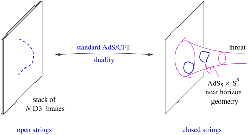
Figure 1.1: Standard AdS/CFT: The left figure shows the description of a stack of D3-branes in terms of open strings (Yang-Mills description), the right figure in terms of closed strings (supergravity description).

In the standard AdS/CFT correspondence [11, 12, 13], a system of $N$ coincident D3-branes is considered within type IIB string theory. Its description in terms of open and closed strings is shown in Fig. 1.1. At low energies massive string modes decouple and the effective theory generated by open string modes is ${\cal N}=4$ $SU(N)$ super Yang-Mills theory in 3+1 dimensions which is known to be a conformal field theory. This theory is located on the world-volume of the D3-branes.

The holographic dual theory is generated by massless closed string modes. In the Maldacena limit, the metric of the D3-branes reduces to its near-horizon (throat) region which is $AdS_{5}\times S^{5}$. This is a product space of a five-dimensional Anti-de-Sitter space and a five-sphere. Closed strings in the asymptotic flat region decouple from the theory inside the throat region.

So far only very little is known about string theory quantization on a curved background including $AdS_{5}\times S^{5}$. One therefore takes the ’t Hooft limit, sending $N\rightarrow\infty$, while keeping the ’t Hooft coupling $\lambda=4\pi g_{s}N$ fixed. Taking also a large ’t Hooft coupling, $\lambda\gg 1$, the radius of curvature $L^{4}=\lambda\alpha^{\prime}{}^{2}$ of the AdS space becomes large leading to a small curvature (there the string length is much smaller than the size of AdS, so we see particles instead of strings). The full quantum string theory then reduces to classical type IIB supergravity on $AdS_{5}\times S^{5}$.

Thus, at low energies we have two different descriptions of a stack of $N$ D3-branes which are conjectured to be equivalent (at large $\lambda$):

• one in terms of the ${\cal N}=4$ $SU(N)$ super Yang-Mills theory in 3+1 dimensions generated by the massless open string modes,

• the other in terms of type IIB supergravity on $AdS_{5}\times S^{5}$ (with integer flux of the five-form Ramond-Ramond field strength, $N=\int_{S^{5}}F_{5}$) generated by the massless closed string degrees of freedom,

where the parameters of the two theories are related as

$$g_{s}=g_{YM}^{2}\,,\qquad L^{4}=\lambda\alpha^{\prime}{}^{2}\,.$$ (1.1)

Here $g_{s}$ is the string coupling, $g_{YM}$ the Yang-Mills coupling, $L$ the radius of curvature of both AdS space and $S^{5}$, and $\alpha^{\prime}=l_{s}^{2}$ is related to the string tension by $T=1/2\pi\alpha^{\prime}$.

Although a strict proof of the AdS/CFT correspondence is still missing, there is a lot of evidence that there is some truth in it. At least the above stated weak form of the correspondence has been very well tested by now.

Note first that the map between AdS and CFT quantities is given by

$${\cal Z}_{sugra}(\phi_{i})=\left\langle\exp\left(\int d^{4}x\phi_{i}^{0}{\cal O}_{i}\right)\right\rangle\,,$$ (1.2)

where the left-hand side is the supergravity partition function evaluated on the classical solution given by $\phi_{i}$ (which satisfies $\phi_{i}|_{\partial AdS}=\phi_{i}^{0}$) and the right-hand side is the generating function for super Yang-Mills theory. $\phi_{i}^{0}$ denotes the value of the supergravity field $\phi_{i}$ at the boundary, where it acts as a source for the operator ${\cal O}_{i}$. We see that there is a one-to-one correspondence between the operators ${\cal O}_{i}$ and fields $\phi_{i}$. It has been verified [13] that there is a precise match between supergravity fields and so-called BPS operators in the gauge theory. As a consistency check observe that the isometries of the $AdS_{5}\times S^{5}$ space correspond to the symmetries of the conformal field theory. The isometry group $SO(4,2)$ of $AdS_{5}$ is the conformal group in four dimensions, while the isometry group $SO(6)\simeq SU(4)$ of $S^{5}$ is the R-symmetry of ${\cal N}=4$ supersymmetry. More generally, both the supergravity fields as well as the Yang-Mills BPS operators fall in the same multiplets of the supergroup $PSU(2,2|4)$.

Moreover, correlation functions of Yang-Mills operators have been computed via supergravity and compared to field theory results (for a review see [36]). It is quite non-trivial that there is an agreement in the general behaviour of the correlation functions in both computations. Of course, numerical factors usually differ since the field theory correlators are computed at weak coupling, while the AdS computation yields correlators at strong coupling.

It is also interesting to compare the vacuum expectation value of a Wilson loop, which in field theory can be expanded in terms of local operators. It became more and more clear that the fundamental string in AdS is the same as the QCD string of large $N$ Yang-Mills theory. For instance, open strings are (dual to) spin chains of adjoint fields (“gluons”) with fundamental fields (“quarks”) at their ends [50]. We also encounter such operators below (see Ch. 2.5).

There are many other checks and tests of the correspondence, which we cannot review here, all of them supporting the conjecture.

1.2 Holography of defect conformal field theories

A generalization of the AdS/CFT correspondence is obtained by embedding an additional probe brane into the $AdS_{5}\times S^{5}$ background. Depending on the dimension of the probe brane, the dual field theory of this supergravity set-up is then a conformal field theory with a space-time defect. These defect conformal field theories (dCFT) involve fields which are confined to a lower-dimensional subspace of the original four-dimensional space-time. For these dCFT the four-dimensional conformal symmetry is broken to the lower-dimensional conformal group of the defect. A typical Feynman diagram corresponding to the interaction of four-dimensional bulk degrees of freedom with defect fields is shown in Fig. 1.2. As a special case one can also have a “defect” of codimension zero corresponding to flavour in four spacetime dimensions [51]. This will become important later when we discuss mesons in QCD-like theories.

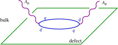
Figure 1.2: Interaction of bulk gauge bosons and defect quarks.

The general problem of introducing a spatial defect into a conformal field theory has been studied in several contexts [52, 53]. Within string theory such defect conformal field theories arise in various brane constructions. They were first studied in this context as matrix model descriptions of compactified NS5-branes [54] and more generally as effective field theories describing various D-brane intersections [55, 56].

The first AdS/CFT setup leading to a dCFT was considered by Karch and Randall in [57, 58, 59]. They conjectured an AdS/CFT duality in which a D5-brane probe (along $x^{0},x^{1},x^{2},x^{4},x^{5},x^{6}$) orthogonally intersects a stack of $N$ D3-branes (along $x^{0},x^{1},x^{2},x^{3}$) on a three-dimensional subspace with coordinates $x^{0},x^{1},x^{2}$, as shown on the left-hand side in Fig. 1.3. The near-horizon limit of this D3-D5 brane system is $AdS_{5}\times S^{5}$ with the D5-brane wrapping an $AdS_{4}\times S^{2}$ submanifold. The supersymmetry of the $AdS_{4}\times S^{2}$ embedding was demonstrated in [60]. The $AdS_{5}$ geometry can be visualized as the interior of a disk as shown on the right-hand side in Fig. 1.3, while the $AdS_{4}$ brane ends on the boundary of the disk.

There are various strings in the set-up: As usual, open string modes with both endpoints on the D3-branes generate the ${\cal N}=4$ super Yang-Mills theory, while closed string modes give rise to type IIB supergravity on $AdS_{5}\times S^{5}$. However, we have additional strings due to the embedding of a probe brane. First, there are strings stretching between the D5-brane and the D3-branes. They give rise to a fundamental hypermultiplet (“quarks”) in the low-energy theory. Due to the decoupling of open strings on the D5-brane in the infrared, the $U(1)$ gauge group on the D5-brane, or $U(N_{f})$ in case of $N_{f}$ D5-branes, turns into the flavour group of the fundamental matter. Second, there are open strings ending on the D5-brane wrapping $AdS_{4}\times S^{2}$. In the probe approximation, one neglects the back-reaction of the D5-brane on the near-horizon background of the D3-branes. Classically, the fluctuation modes of the $AdS_{4}$-brane are then described by the Dirac-Born-Infeld action of the D5-brane (plus Wess-Zumino term).

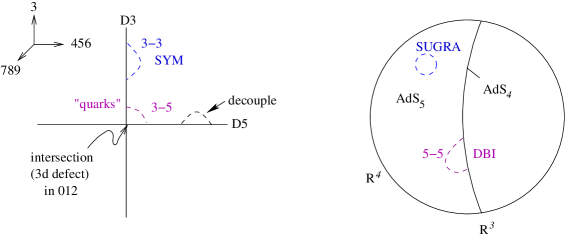
Figure 1.3: Holography of the D3-D5 brane intersection.

Karch and Randall conjecture the AdS/CFT duality to act ‘twice’: First there is the standard AdS/CFT duality between open strings ending on the D3-branes (3-3 strings) and closed strings in type IIB string theory on $AdS_{5}\times S^{5}$. Secondly, they conjecture an additional duality between open strings, stretching between the D5 and D3-branes (3-5 and 5-3 strings), and open strings ending on the D5-brane (5-5 strings) wrapping $AdS_{4}\times S^{2}$.

The world-volume theory of this configuration is a four-dimensional conformal field theory coupled to a codimension one defect. This defect conformal field theory describes the decoupling limit of the D3-D5 intersection, and consists of the ${\cal N}=4$, $d=4$ super Yang-Mills theory coupled to an ${\cal N}=4$, $d=3$ hypermultiplet localized at the defect. In [61] DeWolfe, Freedman and Ooguri constructed the action of the model and developed a precise dictionary between composite operators in the field theory and fluctuation modes on the $AdS_{4}$-brane. In [62], we wrote the action compactly in an ${\cal N}=2,d=3$ superspace and gave field theoretic arguments for quantum conformal invariance.

In summary, the AdS/dCFT correspondence conjectures the equivalence of the following two theories:

4d ${\cal N}=4$ $SU(N)$ type IIB supergravity

super Yang-Mills theory on $AdS_{5}\times S^{5}$         

+                                     $\longleftrightarrow$                            +

3d ${\cal N}=4$ hypermultiplet Dirac-Born-Infeld theory

on $\mathbb{R}^{3}$ defect on $AdS_{4}\times S^{2}$         

Generalization to a general D3-D$p$ intersection

In Ch. 2 we generalize the above duality to the case of a D3-D$p$ brane intersection with $p\in\{(1),3,5,7\}$. The “monopole” case $p=1$ will only be mentioned marginally. Since the D3-D9 intersection is non-supersymmetric, we exclude the case $p=9$. All other D3-D$p$ intersections are supersymmetric and related by T-duality. We also omit the instanton case $p=-1$ since the D(-1)-D3 system does not have a defect interpretation nor does it correspond to an $AdS$ embedding.

The near-horizon geometry is again $AdS_{5}\times S^{5}$ with the D$p$-brane wrapping an $AdS_{k+2}\times S^{k}$ submanifold. Here $k+1=(p+1)/2$ is the dimension of the intersection which agrees with the dimension of the defect. In general, the dual field theory describes the degrees of freedom of the ${\cal N}=4$ $SU(N)$ super Yang-Mills theory coupling to a $k+1$-dimensional defect hypermultiplet in the fundamental representation of the gauge group. The defect breaks supersymmetry by a half. The theory is thus invariant under eight supercharges, i.e. under 2d $(4,4)$, 3d ${\cal N}=4$, or 4d ${\cal N}=2$ supersymmetry in the case of a two-, three-, or four-dimensional defect, respectively.

In the following we give an overview over all D3-D$p$ brane intersections and their corresponding world-volume theories. These configurations are:

D1-D3: The case of $N^{\prime}$ D1-branes ending on a D3-brane has an interpretation in terms of an $SU(N^{\prime})$ magnetic monopole [63]. From the point of view of the effective theory on the D3-brane, the D1-branes act as a point source of magnetic charge for the gauge field. The near-horizon geometry in supergravity is given by an $AdS_{2}$ brane embedded in $AdS_{5}\times S^{5}$. The dual field theory is a four-dimensional defect CFT where the fundamental hypermultiplets are localized on a one-dimensional defect [56, 64]. Two-dimensional conformal field theories with a one-dimensional defect dual to $AdS_{2}$ branes in $AdS_{3}$ have been studied in [65, 66]. However, holography of the D1-D3 system corresponding to an $AdS_{2}$ embedding inside $AdS_{5}$ has not yet been discussed. Since abelian monopoles do not exist, progress towards a holographic description requires the discussion of a non-abelian Dirac-Born-Infeld action of the D1-branes. We will not discuss this case in detail.

In Ch. 2 we will mainly focus on the D3-D3 intersection, for which reason we give a more detailed introduction and an overview over the expected results.

D3-D3: This system, which has first been studied in [67], consists of a stack of D3-branes spanning the $0123$ directions and an orthogonal stack (of D3^′-branes) spanning the $0145$ directions such that eight supercharges are preserved, realising a $(4,4)$ supersymmetry on the common $1+1$ dimensional world-volume. Unlike the D3-D5 intersection, open strings on both stacks of branes remain coupled as $\alpha^{\prime}\rightarrow 0$. However, in the probe approximation a holographic duality can be found relating fluctuations in an $AdS$ background to operators in the dual field theory. One simply takes the number of D3-branes, $N$, in the first stack to infinity, keeping $g_{s}N$ and the number of D3-branes in the second stack, $N^{\prime}$, fixed. In this limit, the ’t Hooft coupling of the gauge theory on the second stack, $\lambda^{\prime}=g_{s}N^{\prime}$, vanishes. Thus the open strings with all endpoints on the second stack decouple, and one is left with a four-dimensional CFT with a codimension two defect. The defect breaks half of the original ${\cal N}=4$, $d=4$ supersymmetry, leaving eight real supercharges realising a two-dimensional $(4,4)$ supersymmetry algebra. The conformal symmetry of the theory is a global $SL(2,R)\times SL(2,R)$, corresponding to a subgroup of the four-dimensional conformal symmetries. The degrees of freedom at the defect are a $(4,4)$ hypermultiplet arising from the open strings connecting the orthogonal stacks of D3-branes.

The classical Higgs branch of this theory has an interpretation as a smooth resolution of the intersection to the holomorphic curve $wy\sim c\alpha^{\prime}$, where $w=X^{2}+iX^{3}$ and $y=X^{4}+iX^{5}$. However, due to the two-dimensional nature of the fields which parameterize these curves, the quantum vacuum spreads out over the entire classical Higgs branch. It has been argued that due to the spreading over the Higgs branch a fully localized supergravity solution for this D3-brane intersection does not exist [68, 69, 70]. Obtaining a closed string description of this defect CFT would therefore seem to be difficult. These objections do not hold in the probe approximation.

In the limit described above, the holographic dual is obtained by focusing on the near horizon region for the first stack of D3-branes, while treating the second stack as a probe. The result is an $AdS_{5}\times S^{5}$ background with $N^{\prime}$ probe D3-branes wrapping an $AdS_{3}\times S^{1}$ subspace. This embedding was shown to be supersymmetric in [60]. We will demonstrate that there is a one complex parameter family of such embeddings, corresponding to the holomorphic curves $wy\sim c$, all of which preserve a set of isometries corresponding to the super-conformal group. As in the D3-D5 system, holographic duality is conjectured to act “twice”. First there is the standard AdS/CFT duality relating closed strings in $AdS_{5}\times S^{5}$ to operators in ${\cal N}=4$ super Yang-Mills theory. Second, there is a duality relating open strings on the probe D$3^{\prime}$ wrapping $AdS_{3}\times S^{1}$ to operators localized on the $1+1$ dimensional defect.

One of the original motivations to search for holographic dualities for defect conformal field theories [57, 58, 59] is that such a duality might imply the localization of gravity on branes in string theory. In the context of a brane wrapping an $AdS_{3}$ geometry embedded inside $AdS_{5}$, localization of gravity would indicate the existence of a Virasoro algebra in the dual CFT, through a Brown-Henneaux mechanism [71]. We do not find any evidence for the existence of a Virasoro algebra in the conformal field theory. Although this theory has a $(4,4)$ superconformal algebra, only the finite part of the algebra is realised in any obvious way. Roughly speaking, the $(4,4)$ superconformal algebra is the common intersection of two ${\cal N}=4,d=4$ superconformal algebras, both of which are finite. The even part of the superconformal group is $SL(2,R)\times SL(2,R)\times SU(2)_{L}\times SU(2)_{R}\times U(1)$, which is also realised as an isometry of the $AdS_{5}$ background which preserves the probe embedding. Enhancement to the usual infinite dimensional algebra would require the existence of a decoupled two-dimensional sector. Correctly addressing this issue would require going beyond the probe limit and studying the back-reaction of the D$3^{\prime}$-branes on the $AdS_{5}\times S^{5}$ geometry as well as gaining a deeper understanding of the dynamics of the defect CFT.

The action for the D3-D3 intersection is most easily and elegantly constructed in $(2,2)$ superspace. Although it may seem unusual to write the ${\cal N}=4,d=4$ components of the action in $(2,2)$ superspace, this is actually quite natural because the four-dimensional supersymmetries are broken by couplings to the defect hypermultiplet. In writing this action, we will not take the limit which decouples one stack of D3-branes. With the help of the manifest chirality of $(2,2)$ superspace we are able to find an argument for the absence of quantum corrections to the combined 2d/4d actions, which implies that the theory remains conformal upon quantization. Although this theory has two-dimensional fields coupled to gauge fields, the gauge couplings are exactly marginal due to the four-dimensional nature of the gauge fields.

We give a detailed dictionary between Kaluza-Klein fluctuations on the probe D3-brane and operators localized on the defect. Of particular interest will be a certain subset of the fluctuations which describe the embedding of the probe inside $AdS_{5}$. This subset is dual to operators containing defect scalar fields, which appear without any derivative or vertex operator structure. Due to strong infrared effects in two dimensions, these fields are not conformal fields associated to states in the Hilbert space. From the point of view of the probe-supergravity system, there is at first sight nothing unusual about these fluctuations. However, upon applying the usual $AdS_{3}$/CFT₂ rules to compute the dual two-point correlator, one finds identically zero due to extra surface terms in the probe action. Thus there is no clear interpretation of these fluctuations as sources for the generating function of the CFT. We shall find however that the bottom of the Kaluza-Klein tower for these fluctuations (with appropriate boundary conditions) parameterizes the aforementioned holomorphic embedding of the probe inside $AdS_{5}$. While the interpretation of this fluctuation as a source is unclear, it nevertheless labels points on the classical Higgs branch. Since the infrared dynamics of two dimensions implies that the vacuum is spread out over the entire Higgs branch, one should in principle sum over holomorphic embeddings when performing computations in the $AdS$ background.

The fluctuations of the probe $S^{1}$ embedding inside $S^{5}$ satisfy the Breitenlohner-Freedman bound despite the lack of topological stability. These fluctuations are dual to a multiplet of scalar operators with defect fermion pairs which we identify with BPS superconformal primaries localized at the intersection. We also find fluctuations of the probe embedding inside $AdS_{5}$ which are dual to descendants of these operators. Remarkably, the AdS computation of the corresponding correlators, which is valid for large ’t Hooft coupling $\lambda$, shows no dependence on $\lambda$. We also study perturbative quantum corrections to the two-point function of the BPS primary operators and find that such corrections are absent at order $g_{YM}^{2}$. Together with the $AdS$ strong coupling result, this suggests the existence of a non-renormalization theorem.

D3-D5: The world-volume theory of this system is a defect CFT with a codimension one defect. Holography of this system was extensively studied in [61]. Historically, it was the first set-up in which defect conformal field theories were studied in AdS/CFT. We reviewed this brane intersection at the beginning of this section (see p. 1.2).

D3-D7: In the D3-D7 brane configuration, first studied by Karch and Katz [51, 72], a spacetime filling D7-brane was added to the $AdS_{5}/{\rm CFT}_{4}$ correspondence. The D7-brane completely fills the $AdS_{5}$ space and wraps a maximal $S^{3}$ inside $S^{5}$. This supergravity configuration is dual to a four-dimensional ${\mathcal{N}}=2$ Yang-Mills theory describing open strings in the presence of one D7 and $N$ D3-branes sharing 3+1 dimensions. The degrees of freedom are those of the ${\mathcal{N}}=4$ super Yang-Mills theory, coupled to an ${\mathcal{N}}=2$ hypermultiplet with fields in the fundamental representation of $SU(N)$. The latter arise from strings stretched between the D7 and D3-branes. This set-up becomes important in the next section, where we discuss flavour in confining supergravity backgrounds corresponding to quarks in four-dimensional non-supersymmetric QCD-like theories.

Holography of defect conformal field theories and the embedding of branes in AdS/CFT have also been considered in various other contexts: Gravitational aspects were discussed in [73, 74, 75, 76]. The Penrose limit of this background was studied in [60, 77], wherein a map between defect operators with large $R$-charge and open strings on a D3-brane in a plane wave background was constructed. RG flows related to defect conformal field theories were discussed in [78]. Finally, defect CFT’s were discussed in connection with the phenomenon of supertubes in [79]. The dCFT on the D3-D5 intersection in connection to integrable open spin chains was studied in [50]. Further related papers not mentioned so far are [80, 81, 82, 83, 84, 85].

1.3 Meson spectra in AdS/CFT and spontaneous chiral symmetry breaking

In the previous section we have seen how matter in the fundamental representation of the gauge group can be introduced in AdS/CFT via the embedding of a probe brane in $AdS_{5}\times S^{5}$. The corresponding D3-D$p$ brane intersection accommodates the holographic dual (defect) conformal field theory on its world-volume.

The D3-D7 configuration is special since fundamental fields are allowed to propagate in all four space-time dimensions. This opens up the possibility for studying flavour in supersymmetric extensions of QCD. It is possible to introduce mass for the fundamental matter by separating the D7-brane from the D3-branes. The dual description involves a probe D7 on which the induced metric is only asymptotically $AdS_{5}\times S^{3}$. In this case there is a discrete spectrum of mesons. This spectrum has been computed (exactly!) at large ’t Hooft coupling [86] using an approach analogous to the glueball calculations in deformed AdS backgrounds. The novel feature here is that the “quark” bound states are described by the scalar fields in the Dirac-Born-Infeld action of the D7-brane probe.

In view of a gravity description of Yang-Mills theory with confined quarks, it is natural to attempt to generalize these calculations to probes of deformed AdS spaces. For instance in [87], a way to embed D7-branes in the Klebanov-Strassler (KS) background [88] was found, following the suggestion of [51]. Moreover in [87], the spectrum of mesons dual to fluctuations of the D7-brane probe in the KS-geometry was calculated. The underlying theory is an ${\mathcal{N}}=1$ gauge theory with massive chiral superfields in the fundamental representation. Calculations of meson spectra for ${\cal N}=1$ supersymmetric gauge theories have also been performed in [89, 90, 91]. Related work may also be found in [92, 93].

One of the most important features of QCD dynamics is chiral symmetry breaking by a quark condensate, but since this is forbidden by unbroken supersymmetry, these constructions do not let us address this issue. In Ch. 3, we attempt to come somewhat closer to QCD by considering the embedding of D7-branes in two non-supersymmetric backgrounds which exhibit confinement. Although neither of these backgrounds corresponds exactly to QCD since they contain more degrees of freedom than just gluons and quarks, we might nevertheless expect chiral symmetry breaking behaviour. The quark mass $m$ and the quark condensate expectation value $c$ are given by the UV asymptotic behaviour of the solutions to the supergravity equations of motion in the standard holographic way (see [94] for an example of this methodology). In the ${\cal N}=2$ supersymmetric Karch-Katz scenario [51] with a D7 probe in standard AdS space, we show that there cannot be any regular solution which has $c\neq 0$; the supersymmetric theory does not allow a quark condensate. We then find that for the deformed AdS backgrounds we consider, there are regular solutions with $c\neq 0$. The case $c\neq 0$ with $m=0$ corresponds to spontaneous chiral symmetry breaking.

The first supergravity background we consider is the Schwarzschild black hole in $AdS_{5}\times S^{5}$. In the absence of D7-branes, this background is dual to strongly coupled ${\mathcal{N}}=4$ super Yang-Mills at finite temperature and is in the same universality class as three-dimensional pure QCD [16]. Glueball spectra in this case were computed in [95, 24]. We introduce D7-branes into this background and compute the quark condensate as a function of the bare quark mass, as well as the meson spectrum. This background is dual to the finite temperature version of the ${\mathcal{N}}=2$ super Yang-Mills theory considered in [51, 86]. The finite temperature ${\mathcal{N}}=2$ theory is not in the same universality class as three-dimensional QCD with light quarks since the antiperiodic boundary conditions for fermions in the Euclidean time direction give a non-zero mass to the quarks upon reduction to three-dimensions, even if the hypermultiplet mass of the underlying ${\mathcal{N}}=2$ theory vanishes. In fact these quarks decouple if one takes the temperature to infinity in order to obtain a truly three-dimensional theory. Nevertheless at finite temperature the geometry describes an interesting four-dimensional strongly coupled gauge configuration with quarks. The meson spectrum we obtain has a mass gap of order of the glueball mass. Furthermore we find that the $\bar{\Psi}\Psi$ condensate vanishes for zero hypermultiplet mass, such that there is no spontaneous violation of parity in three dimensions or chiral symmetry in four dimensions. However for $m\neq 0$ we find a condensate $c$ which at first grows linearly with $m$, and then shrinks back towards zero. Increasing $m$ further, the D7 embedding undergoes a geometric transition at a critical mass $m_{c}$. At sufficiently large $m\gg m_{c}$ the condensate is negligible and the spectrum matches smoothly with the one found in [86] for the ${\mathcal{N}}=2$ theory. Our numerics give some evidence that the geometric transition corresponds to a first order phase transition in the dual gauge theory, at which the condensate $c(m)$ is discontinuous.

The second non-supersymmetric background which we consider was found by Constable and Myers [20]. This background is asymptotically $AdS_{5}\times S^{5}$ but has a non-constant dilaton and $S^{5}$ radius. In the field theory an operator of dimension four with zero R-charge has been introduced (such as ${\rm tr}\,F^{\mu\nu}F_{\mu\nu}$). This deformation does not give mass to the adjoint fermions and scalars of the underlying ${\mathcal{N}}=4$ theory but does leave a non-supersymmetric gauge background. Furthermore, unlike the AdS black-hole background, the geometry has a naked singularity. Nevertheless, in a certain parameter range, this background gives an area law for the Wilson loop and a discrete spectrum of glueballs with a mass gap.

We obtain numerical solutions for the D7-brane equations of motion in the Constable-Myers background with asymptotic behaviour determined by a quark mass $m$ and chiral condensate $c$. We compute the condensate $c$ as a function of the quark mass $m$ subject to a regularity constraint. Remarkably, our results are not sensitive to the singular behaviour of the metric in the IR. For a given mass there are two regular solutions of which the physical, lowest action solution corresponds to the D7-brane “ending” before reaching the curvature singularity. Of course the D7-brane does not really end, however the $S^{3}$ about which it is wrapped contracts to zero size, similarly to the scenario discussed in [51]. In our case the screening of the singularity is related to the existence of the condensate. Furthermore we find numerical evidence for a non-zero condensate in the limit $m\rightarrow 0$. This corresponds to spontaneous breaking of the $U(1)$ chiral symmetry which is non-anomalous in the large $N$ limit [96] (for a review see [97]).

We also compute the meson spectrum by studying classical fluctuations about the D7-embedding. For zero quark mass, the meson spectrum contains a massless mode, as it must due to the spontaneous chiral symmetry breaking. Note that since the spontaneously broken axial symmetry is $U(1)$ for a single D7-brane, the associated Goldstone mode is a close cousin to the $\eta^{\prime}$ of QCD, which is a Goldstone boson in the large $N$ limit. We briefly comment on generalizations to the case of more than one flavour or, equivalently, more than one D7-brane. Moreover we give a holographic version of the Goldstone theorem.

The main message of this part of the paper is that non-supersymmetric gravity duals of gauge theories dynamically generate quark condensates and can break chiral symmetries. We stress that the physical interpretation of naked singularities is a delicate issue, for instance in the light of the analysis of [98]. This applies in particular to the discussion of light quarks and mesons. It is therefore an important part of our analysis that in the presence of a condensate the physical solutions to the supergravity and DBI equations of motion never reach the singularity in the IR. Of course it would be interesting to understand this mechanism further and to see if it occurs in other supergravity backgrounds as well.

Subsequent to [99, 100], chiral symmetry breaking in a non-supersymmetric background obtained from type IIA string theory has been found in [101]. Chiral symmetry breaking in the Constable-Myers background has been studied further in [102].

1.4 Deconstruction of extra dimensions

In the last section we have seen that by relating a five-dimensional gravitational theory to a four-dimensional quantum field theory, AdS/CFT introduces an extra dimension in a natural way. Another possibility to generate extra dimensions is given by the deconstruction technique. In Ch. 4 we apply the deconstruction method to the dCFT of intersecting D3-branes for which the AdS dual is discussed in Ch. 2. Generating two compact extra-dimensions in this system, we obtain a discrete field theory description for intersecting M5-branes wrapped on a two-torus. Due to the obstructions of finding a continuous lagrangian description of M5-branes, the M5-M5 intersection is not very well understood at present. We demonstrate that deconstruction is able to contribute to the understanding of intersecting M5-branes.

Deconstruction is a method to generate (discrete) extra dimensions in theories with internal gauge symmetries. This innovative method has been developed by Arkani-Hamed, Cohen and Georgi [103] and, independently, by Hill, Pokorski and Wang [104] (for early work on this subject, see [105, 106]). The deconstruction method has been used in many fields in theoretical high energy physics and phenomenology. For instance, lattice gauge theorists make use of the discrete nature of the generated extra dimensions to study supersymmetric theories on the lattice [107]. In phenomenology, deconstruction and the physics of so-called theory spaces play an important role in stabilizing the electro-weak scale, see [103] and references thereof. In these models the Higgs boson appears as a pseudo-Goldstone boson protecting the Higgs mass. In the context of quantizing gravity, physicists also got interested in the generation of discrete gravitational dimensions in Einstein’s General Relativity [108, 109, 110, 111, 112]. Amongst many other subjects these examples demonstrate the broad application of deconstruction and the universality of this method.

Subsequent to these developments Arkani-Hamed et al [113] published a further pioneering work, which made deconstruction highly interesting for string theorists. String theory predicts the existence of non-gravitational theories in five and six dimensions, even though no consistent Lagrangians are known for interacting theories in these dimensions. These theories have been discovered by some limit of string theory configurations involving five-branes. A particularly interesting example is the six-dimensional theory with $(2,0)$ supersymmetry describing the decoupling limit of multiple parallel M5-branes [114]. Although this theory is believed to be a local quantum field theory, obstructions to finding a Lagrangian description arise because of difficulties in constructing a non-abelian generalization of a chiral two-form (see for example [115]). The spectrum includes tensionless BPS strings, which are in some sense the “off-diagonal” excitations of the non-abelian chiral two-form. Until recently, the only known formulation of this theory was in terms of a matrix model describing its discrete light cone quantization [116].

Recently, a formulation was found [113, 117] using the deconstruction technique: In order to obtain a description for the six-dimensional superconformal theory located on M5-branes, one considers the low-energy effective theory of a stack of $kN$ D3-branes at an orbifold of the type $\mathbb{C}^{2}/\mathbb{Z}_{k}$. The resulting theory is a ${\cal N}=2$ four-dimensional super Yang-Mills theory with a product gauge group $SU(N)^{k}$ whose field content is given by the (quiver) diagram shown in Fig. 1.4.

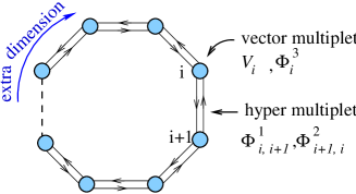
Figure 1.4: Theory space (quiver diagram) for parallel D3-branes at a $\mathbb{C}^{2}/\mathbb{Z}_{k}$ orbifold. Each node corresponds to an ${\cal N}=2$ vector multiplet, while double lines between neighboring nodes correspond to an ${\cal N}=2$ hypermultiplet.

Each of the sites is associated with one of the $k$ $SU(N)$ gauge groups and represents a vector multiplet $V_{i}$ as well as an adjoint chiral multiplet $\Phi^{3}_{i}$ ($i=1,...,k$) which together form a ${\cal N}=2$ vector multiplet. Two neighbouring sites are connected by two oppositely oriented links representing the complex scalars $\Phi^{1}_{i,i+1}$ and $\Phi^{2}_{i+1,i}$ which together form a ${\cal N}=2$ hyper multiplet $(\Phi^{1},{\bar{\Phi}}^{2})_{i,i+1}$. It can now be argued that at low-energies (on the Higgs branch) this particular field theory generates two extra dimensions. This means that the theory, which is four-dimensional at high energies, behaves as a six-dimensional theory at low energies, in which the two extra dimensions are compactified on a discrete toroidal lattice. Such a lattice with sites and link fields is called a theory space.

It is not possible to make further statements about this six-dimensional theory unless one considers the string theory in more detail from which the above field theory descends in a low-energy limit. A string theoretical analysis shows that the Higgs branch of the field theory corresponds to moving the D3-branes a finite distance away from the orbifold singularity, where they become M5-branes after an appropriate T-duality and lift to M-theory. The deconstructed six-dimensional theory can therefore be identified with the world-volume theory of M5-branes, which is the 6d (2, 0) superconformal field theory. In Sec. 4.3 we will review the deconstruction of the non-abelian M5-brane action in much more detail.

In this paper we extend the above deconstruction to the case of intersecting M5-branes, about which even less is known. For details of this deconstruction please see Sec. 4.4 which is based on [118, 119]. We will study further the defect conformal field theory associated with two stacks of D3-branes intersecting each other over a 1+1-dimensional subspace. This brane configuration is placed at a $\mathbb{C}^{2}/\mathbb{Z}_{k}$ orbifold, such that the supersymmetry of the defect conformal field theory is broken to $(4,0)$. Applying the method of deconstruction of [113] generates two extra compact dimensions in an appropriate $k\rightarrow\infty$ limit. In this way we generate a low-energy description of two intersecting stacks of M5 branes. By identifying moduli of the M5-M5 intersection in terms of those of the defect CFT, we will argue that the $SU(2)_{L}$ R-symmetry of the $(4,0)$ defect CFT matches the $SU(2)$ R-symmetry of the ${\cal N}=2,d=4$ theory of the M5-M5 intersection. An amazing result is that the intersection is described by a four-dimensional tensionless string-theory.

In Sec. 4.5 we finally elaborate on the fascinating idea to find a four-dimensional Yang-Mills theory which generates seven extra-dimensions on its Higgs branch such that it is able to describe M-theory itself. This section is based on [120]. We propose to deconstruct M-theory from a four-dimensional non-supersymmetric quiver gauge theory with gauge group $SU(N)^{N_{4}N_{6}N_{8}}$ and $N_{4,6,8}$ three positive integers. The corresponding orbifold realisation is given by a stack of D3-branes in type IIB string theory placed at the origin of $\mathbb{C}^{3}/\Gamma$, where the orbifold group $\Gamma$ is the product of three cyclic groups $\mathbb{Z}_{N_{4}}\times\mathbb{Z}_{N_{6}}\times\mathbb{Z}_{N_{8}}$. The quiver diagram is a discretized three-torus with a body-centred cubic lattice structure.

At a certain point in the moduli space, each of the $\mathbb{Z}_{N}$ factors generates a circular discretized extra dimension. In an appropriate $N_{4,6,8}\rightarrow\infty$ limit, the extra dimensions become continuous, such that the theory appears to be seven-dimensional on the Higgs branch (corresponding to the world-volume theory of D6-branes). There is however a peculiarity in this deconstruction which suggests that the strongly coupled Higgs branch theory is actually an eleven-dimensional gravitational theory: The deconstructed seven-dimensional gauge theory breaks down at a cut-off $\Lambda_{\rm 7d}$. It requires an ultra-violet completion which by string theory arguments can be shown to be M-theory on an $A_{N-1}$ singularity (the M-theory lift of D6-branes). This suggests the equivalence of M-theory on $A_{N-1}$ with the continuum limit of the Higgs branch of the present quiver theory.

The equivalence is also supported by the following properties of the quiver theory on the Higgs branch. We find Kaluza-Klein states in the spectrum of massive gauge bosons which are responsible for the generation of three extra dimensions. Since in M-theory on $A_{N-1}$ the gauge theory is localized at the singularity which is a seven-dimensional submanifold, we can see three of the seven extra dimensions in the gauge boson spectrum. Moreover, we identify states in the spectrum of massive dyons which are identical to M2-branes wrapping two of the three compact extra dimensions.

For further applications of deconstruction in string theory see Refs. [121, 122, 123, 124, 125, 126, 127, 128, 129, 130].

2 Defect conformal field theories and holography

In this chapter we study holography of the D3-D$p$ brane intersection introduced in Ch. 1. The results on the probe-supergravity side of the correspondence hold for all $p\in\{3,5,7\}$. The dual (defect) conformal field theory can most conveniently be described in terms of $k+1$-dimensional superfields. Without loosing to much generality, we specialize the field theory discussion to the case of intersecting D3-branes (i.e. $p=3$ and $k=1$) which is formulated in a two-dimensional superspace. Not only that this theory is interesting by itself as an example of a defect conformal field theory, in Ch. 4 we will need it again for studying intersecting M5-branes. The D3-D5 intersection can be described in an analogous approach using a three-dimensional superspace formalism [62] or component notation [61]. The D3-D7 intersection is a degenerate “defect” conformal field theory with a codimension zero defect. The corresponding field theory can easily be formulated in an ${\cal N}=1$ four-dimensional superspace and will be discussed in Ch. 3.

This chapter is organised as follows. In Sec. 2.1 we present the D3-D$p$ brane setup and its dual description in terms of lower-dimensional AdS-branes in $AdS_{5}$. In Sec. 2.2 we obtain the spectrum of low-energy fluctuations about the probe geometry. In Sec. 2.3 we determine the dependence of general n-point functions associated with these fluctuations on the ’t Hooft coupling. We compute one-point functions and bulk-defect two-point functions and show that their scaling behaviour agrees with the general structure fixed by conformal invariance. In Sec. 2.4 we study the field theory associated with the intersecting D3-branes. In Sec. 2.5 we focus on some peculiarities of the D3-D3 intersection which are due to the two-dimensional conformal symmetry on the defect. For instance, we show that the two-point correlators of a special class of defect operators do not have the usual power-law behaviour. Moreover we discuss the classical Higgs branch of intersecting D3-branes and derive the fluctuation-operator dictionary for the conjectured AdS/CFT correspondence. We also demonstrate that two-point functions of the BPS primary operators do not receive any radiative corrections to order $g^{2}$, thus providing evidence for a non-renormalization theorem.

2.1 Holography for the D3-D$p$ brane intersection

2.1.1 The D3-D$p$ brane configuration

We are interested in the conformal field theory describing the low energy limit of a stack of $N$ D3-branes in the $x^{0},x^{1},x^{2},x^{3}$ directions intersecting another stack of $N^{\prime}$ D$p$-branes, where $p\in\{1,3,5,7\}$. Depending on $p$ the stack of D$p$-branes is aligned in the directions, as indicated in the following table:

D$p$	0	1	2	3	4	5	6	7	8	9
D1	X				X
D$3$	X	X			X	X
D$5$	X	X	X		X	X	X
D$7$	X	X	X	X	X	X	X	X

Orthogonal D$p$–D$q$ brane intersections preserve 8 supercharges, i.e. $1/4$ of the maximal supersymmetry, if $p$ and $q$ fulfill the condition, see e.g. [131],

$$p+q-2k=0\,\,{\rm mod}\,\,4\,,$$ (2.1)

with $k$ the number of intersecting (spatial) dimensions. The D$3$–D$p$ intersections have $q=3$ and $k=(p-1)/2$ such that Eq. (2.1) is automatically satisfied.

The massless open string degrees of freedom of the D$3$–D$p$ intersection correspond to a ${\cal N}=4$ super-Yang-Mills multiplet (generated by 3-3 strings) coupled to a fundamental hypermultiplet (3-$p$ and $p$-3 strings) localized at the $k+1$-dimensional intersection. The decoupling of closed strings is achieved by scaling $N\rightarrow\infty$ while keeping the ’t Hooft coupling $\lambda\equiv g^{2}_{YM}N=4\pi g_{s}N$ fixed. This is the usual ’t Hooft limit for the gauge theory describing the $N$ D3-branes. The ’t Hooft coupling for the $N^{\prime}$ orthogonal D$p$-branes is

$$\lambda^{\prime}=2(2\pi)^{p-2}g_{s}l_{s}^{p-3}N^{\prime}=\lambda(2\pi l_{s})^{p-3}N^{\prime}/N$$ (2.2)

which vanishes in the above limit if $N^{\prime}$ is kept fixed. This implies that the $SU(N^{\prime})$ gauge theory on the D$p$-branes (generated by $p$-$p$ strings) decouples and the group $SU(N^{\prime})$ becomes the flavour symmetry of $N^{\prime}$ flavours. For $\lambda\ll 1$ the appropriate description of this system is given by a four-dimensional ${\cal N}=4$ $SU(N)$ gauge theory coupled to $N^{\prime}$ hypermultiplets at a $k+1$ dimensional defect. The D3-D$p$ intersection and the decoupling of strings is shown on the right hand side of Fig. 2.1.

For $\lambda\gg 1$ one may replace the $N$ D3-branes by the geometry $AdS_{5}\times S^{5}$, according to the usual AdS/CFT correspondence. The D$p$-branes may be treated as a probe of the $AdS_{5}\times S^{5}$ geometry. Comparing the tension of both stacks of branes,

$$T_{Dp}=\frac{\nu}{(2\pi l_{s})^{p-3}}\,T_{D3}\,\qquad(\nu=N^{\prime}/N)\,,$$ (2.3)

we see that the tension $T_{Dp}$ and thus the backreaction of the D$p$-branes can be neglected in the probe limit $\nu\rightarrow 0$ keeping $\nu/l_{s}^{p-3}\ll 1$. As we will see shortly, the D$p$-branes act as $AdS_{k+2}\times S^{k}$ probe branes. Consequently, for large ’t Hooft coupling, the generating function for correlation functions of the defect CFT should be given by the classical action of IIB supergravity on $AdS_{5}\times S^{5}$ coupled to a Dirac-Born-Infeld theory on $AdS_{k+2}\times S^{k}$. The $AdS$ brane embedding in $AdS_{5}\times S^{5}$ is shown on the left hand side of Fig. 2.1.

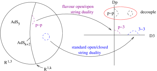
Figure 2.1: AdS/CFT duality for an defect CFT. The duality acts twice. Once for the IIB supergravity on $AdS_{5}\times S^{5}$, and once for DBI theory on $AdS_{k+2}\times S^{k}$.

Following the arguments of [57, 58, 59, 61] we propose that the AdS/CFT duality “acts twice” in the background with an $AdS_{k+2}$-brane embedded in $AdS_{5}$. This means that the closed strings on $AdS_{5}$ should be dual to ${\cal N}=4$ $SU(N)$ super Yang-Mills theory on $\mathbb{R}^{1,3}$, while open string modes on the probe $AdS_{k+2}$-brane should be dual to the fundamental hypermultiplet on the $\mathbb{R}^{1,k}$ defect (see Fig. 2.1). Interactions between the defect hypermultiplet and the bulk ${\cal N}=4$ fields should correspond to couplings between open strings on the probe D$p$-brane and closed strings in $AdS_{5}\times S^{5}$.

2.1.2 AdS-branes in $AdS_{5}\times S^{5}$

We now demonstrate the existence of a one complex parameter family of $AdS_{k+2}\times S^{k}$ embeddings of the probe D$p$-branes in the $AdS_{5}\times S^{5}$ background. Consider first the geometry of the stack of $N$ D3-branes before taking the near horizon limit. The D3 metric is given by

$$ds^{2}=\left(1+\frac{L^{4}}{r^{4}}\right)^{-\frac{1}{2}}(-dt^{2}+dx_{1}^{2}+dx_{2}^{2}+dx_{3}^{2})+\left(1+\frac{L^{4}}{r^{4}}\right)^{\frac{1}{2}}(dx_{4}^{2}+\cdots+dx_{9}^{2})\,,$$ (2.4)

with $r^{2}=x_{4}^{2}+...+x_{9}^{2}$. The probe sits at the origin of the space transverse to its world-volume. With this choice of embedding the induced metric on the probe world-volume is

$$ds^{2}_{probe}=h^{-1/2}\left(-dx_{0}^{2}+...+dx_{k}^{2}\right)+h^{1/2}d\vec{y}^{2}$$ (2.5)

where $h=1+L^{4}/|\vec{y}|^{4}$ ($y^{2}=x_{4}^{2}+...+x_{4+k}^{2}$) is the harmonic function appearing in the background geometry evaluated at the position of the probe. In the near horizon limit, $L/r\gg 1$, the D3-brane geometry becomes $AdS_{5}\times S^{5}$,

$$ds^{2}_{AdS_{5}\times S^{5}}= \frac{L^{2}}{u^{2}}(-dt^{2}+dx_{1}^{2}+dx_{2}^{2}+dx_{3}^{2}+du^{2})\hskip 45.52458pt$$ (2.6)

$$+L^{2}\left(d\phi^{2}_{5}+s_{\phi_{5}}^{2}d\phi_{4}^{2}+s_{\phi_{5}}^{2}s_{\phi_{4}}^{2}d{\phi_{3}}^{2}+s_{\phi_{5}}^{2}s_{\phi_{4}}^{2}s_{\phi_{3}}^{2}d{\phi_{2}}^{2}+s_{\phi_{5}}^{2}s_{\phi_{4}}^{2}s_{\phi_{3}}^{2}s_{\phi_{2}}^{2}d{\phi_{1}}^{2}\right),$$

where $u\equiv\frac{L^{2}}{r}$ and we have defined angular variables $\phi_{1},{\phi_{2}},{\phi_{3}},{\phi_{4}},{\phi_{5}}$ via

$$x^{4} =rs_{\phi_{5}}s_{\phi_{4}}s_{\phi_{3}}s_{\phi_{2}}s_{\phi_{1}} x^{5}=rs_{\phi_{5}}s_{\phi_{4}}s_{\phi_{3}}s_{\phi_{2}}c_{\phi_{1}}\,,$$

$$x^{6} =rs_{\phi_{5}}s_{\phi_{4}}s_{\phi_{3}}c_{\phi_{2}}\,, x^{7}=rs_{\phi_{5}}s_{\phi_{4}}c_{\phi_{3}}\,,$$

$$x^{8} =rs_{\phi_{5}}c_{\phi_{4}}\,, x^{9}=rc_{\phi_{5}}\,,$$ (2.7)

where $s_{\phi_{1}}=\sin\phi_{1}$, $c_{\phi_{1}}=\cos{\phi_{1}}$ etc. It is instructive to consider this limit from the point of view of the probe metric. One can easily show that in the near-horizon region the induced metric on the probe becomes

$$ds^{2}_{probe}=\frac{{L}^{2}}{\tilde{u}^{2}}\left(-dx^{2}_{0}+...+dx_{k}^{2}+d\tilde{u}^{2}\right)+{L^{2}}d\Omega_{k}^{2}\,,$$ (2.8)

where $\tilde{u}=u|_{x^{5+k},...,x^{9}=0}$. One immediately recognizes Eq. (2.8) as the metric on $AdS_{k+2}\times S^{k}$ with radius of curvature ${L}$. The probe wraps a $k$-sphere $S^{k}$ of maximal radius inside the $S^{5}$. We summarize the AdS-branes in Tab. 2.1.

D1:	$(0|$ D1 $\perp$ D3)	$AdS_{2}$
D3:	$(1|$ D3 $\perp$ D3)	$AdS_{3}\times S^{1}$
D5:	$(2|$ D5 $\perp$ D3)	$AdS_{4}\times S^{2}$
D7:	$(3|$ D7 $\perp$ D3)	$AdS_{5}\times S^{3}$

Table 2.1: AdS-brane embeddings in $AdS_{5}\times S^{5}$ which preserve 8 supercharges. $(k|$ Dp $\perp$ D3) denotes the D3-D$p$ brane intersection on $k$ spatial dimensions.

The boundary of the embedded $AdS_{k+2}$-brane is a $k+1$-dimensional Minkowski space $\mathbb{R}^{1,k}$ at $\tilde{u}=0$, and lies within the $\mathbb{R}^{1,3}$ boundary of $AdS_{5}$. This embedding is indeed supersymmetric, as was verified in [60]. Thus this configuration is stable despite the fact that the $S^{k}$ is contractible within the $S^{5}$. As we will see in Sec. 2.2.2, the naively unstable modes associated with contracting the $S^{k}$ satisfy the Breitenlohner-Freedman bound [132] for scalars in $AdS_{k+2}$, and therefore do not lead to an instability.

2.1.3 Isometries

In the absence of the (probe) D$p$-branes, the isometry group of the $AdS_{5}\times S^{5}$ background is $SO(2,4)\times SO(6)$. The $SO(2,4)$ component acts as conformal transformations on the boundary of $AdS_{5}$, while the $SO(6)\simeq SU(4)$ isometry of $S^{5}$ is the R-symmetry of four-dimensional ${{\cal N}=4}$ super Yang-Mills theory, under which the six real scalars $X^{4,5,6,7,8,9}$ transform in the vector representation.

In the presence of the D$p$-branes, the $AdS_{5}\times S^{5}$ isometries are broken to the subgroup which leaves the embedding equations of the D$p$-branes invariant:

$$SO(2,4)\times SO(6)\rightarrow SO(2,k+1)\times SO(3-k)\times SO(k+1)\times SO(5-k)$$ (2.9)

Out of the $SO(2,4)$ isometry of $AdS_{5}$ only $SO(2,k+1)\times SO(3-k)$ is preserved. The $SO(2,k+1)$ factor is the isometry group of $AdS_{k+2}$, while the $SO(3-k)$ factor (non-trivial only for $k=0,1$) acts as a rotation of the coordinates $X^{k+1},...,X^{3}$. Out of the $SO(6)\simeq SU(4)$ isometry of $S^{5}$, only $SO(k+1)\times SO(5-k)$ is preserved. The $SO(k+1)$ factor here rotates the $S^{k}$ of the D$p$-brane world-volume. The $SO(5-k)$ component acts on the coordinates $X^{5+k,...,9}$.

2.2 Fluctuations in the probe-supergravity background

Following the conjecture put forth in [57, 58, 59] and elaborated upon in [61], we expect the holographic duals of defect operators localized on the intersection are open strings on the D$p$-branes, whose world-volume is an $AdS_{k+2}\times S^{k}$ submanifold of $AdS_{5}\times S^{5}$. The operators with protected conformal dimensions should be dual to probe Kaluza-Klein excitations at “sub-stringy” energies, $m^{2}\ll\lambda/L^{2}$. In this section we shall find the mass spectra of these excitations. Later we will find this spectrum to be consistent with the dimensions of operators localized on the intersection.

2.2.1 The probe-supergravity system

The full action describing physics of the background as well as the probe is given by

$$S_{bulk}=S_{IIB}+S_{DBI}+S_{WZ}\,.$$ (2.10)

The contribution of the bulk supergravity piece of the action in Einstein frame is

$$S_{IIB}=\frac{1}{2\kappa^{2}}\int d^{10}x\sqrt{-g}\left(R-\frac{1}{2}e^{2\Phi}(\partial\Phi)^{2}+\cdots\right)\,,$$ (2.11)

where $2\kappa^{2}=(2\pi)^{7}g_{s}^{2}l_{s}^{8}$. The dynamics of the probe D$p$-brane is given by a Dirac-Born-Infeld term and a Wess-Zumino term [133],

$$S =S_{DBI}+S_{WZ}\,,$$ (2.12)

where

$$S_{DBI} =-T_{Dp}\int d^{p+1}\sigma e^{-\Phi}\sqrt{-\det\left(g_{ab}^{PB}+e^{-\Phi/2}{\cal F}_{ab}\right)}\,.$$ (2.13)

The brane tension $T_{Dp}$ is given by $T_{Dp}=(g(2\pi)^{p}\alpha^{\prime(p+1)/2})^{-1}$ with $g=\kappa/(8\pi^{7/2}\alpha^{\prime}{}^{2})$. The metric $g_{ab}^{PB}$ is the pull back of the bulk $AdS_{5}\times S^{5}$ metric to the world-volume of the probe. ${\cal F}_{ab}=B_{ab}+2\pi l_{s}^{2}F_{ab}$ is the total world-volume field strength. The Wess-Zumino action $S_{WZ}$ will be discussed in Sec. 2.2.4.

We work in a static gauge where the world-volume coordinates of the brane are identified with the space time coordinates by $\sigma^{a}\sim x^{0},...,x^{k},u,\phi_{1},...,\phi_{k}$. With this identification the DBI action is

$$S_{DBI}=-T_{Dp}\int d^{p+1}\sigma\sqrt{-\det\left(g_{ab}+\partial_{a}Z^{i}\partial_{b}Z^{j}g_{ij}+{\cal F}_{ab}+2g_{ai}\partial_{b}Z^{i}\right)}\,,$$ (2.14)

where $i,j$ label the transverse directions to the probe and the scalars $Z^{i}$ represent the fluctuations of the transverse scalars $X^{k+1},...,X^{3},\phi_{k+1},...,\phi_{5}$. Also, $e^{-\Phi}=g_{s}^{-1}=1/g_{YM}^{2}$ has been set to one. Henceforth we will only consider the open string fluctuations on the probe and thus drop terms involving closed string fields $B_{ab}$ and $g_{ai}$. The embedding conditions of the $AdS_{k+2}$-brane are given by

$$X^{k+1}=...=X^{3}=0\,,\qquad\phi_{k+1}=...=\phi_{5}=\frac{\pi}{2}\,,$$ (2.15)

where the conditions on the $\phi_{i}$ are equivalent to $X^{k+5}=...=X^{9}=0$, as can be seen from Eq. (2.7). The $AdS$-brane wraps a maximal $k$-sphere $S^{k}$ inside $S^{5}$. To quadratic order in fluctuations, the action takes the form

$$S_{DBI}=-T_{Dp}L^{p+1}\int d^{p+1}\sigma\sqrt{\bar{g}_{p+1}} \left[1+\sum_{i=k+1}^{5}(\frac{1}{2}\partial_{a}\phi^{\prime}_{i}\partial^{a}\phi^{\prime}_{i}-\frac{k}{2}{\phi^{\prime}}_{i}^{2})\right.$$ (2.16)

$$\left.+\sum_{i=k+1}^{3}\frac{1}{2u^{2}}\partial_{a}X^{i}\partial^{a}X^{i}+\frac{1}{4}(2\pi l_{s}^{2})^{2}F_{ab}F^{ab}\right]\,,$$

where $\phi^{\prime}_{i}\equiv\phi_{i}-\frac{\pi}{2}$ and $\bar{g}_{p+1}$ is the determinant of the rescaled $AdS_{k+2}\times S^{k}$ metric $\bar{g}^{p+1}_{ab}$ given by

$$d\bar{s}^{2}=\frac{1}{{u}^{2}}\left(-dt^{2}+...+dx_{k}^{2}+d{u}^{2}\right)+d\Omega_{k}^{2}\,.$$ (2.17)

2.2.2 $S^{k}$ fluctuations inside $S^{5}$

From Eq. (2.16) we see that the angular fluctuations $\phi^{\prime}_{k+1},...,\phi^{\prime}_{5}$ are minimally coupled scalars on $AdS_{k+2}\times S^{k}$ satisfying the equation of motion

$$(\Box+k)\phi^{\prime}=0\,,\quad{\rm with}\quad\Box=\Box_{AdS}+\Box_{S^{k}}\,.$$ (2.18)

Interestingly they have $m^{2}=-k$ which, although negative, satisfies (saturates for $k=1$) the Breitenlohner-Freedman bound $m^{2}\geq-d^{2}/4$, where $d=k+1$ for $AdS_{k+2}$. We can separate variables by means of the ansatz

$$\phi^{\prime}=\phi^{\prime}_{l}(\vec{x},u){\cal Y}^{l}(S^{k})\,,$$ (2.19)

where the spherical harmonics on $S^{k}$ satisfy

$$\Box_{S^{k}}{\cal Y}^{l}=-l(l+k-1){\cal Y}^{l}\,$$ (2.20)

with $\Box_{S^{k}}$ the Laplacian on the $k$-sphere $S^{k}$. For the Kaluza-Klein modes of these scalars we then find the masses $m^{2}=-k+l(l+k-1)$. This leads to a spectrum of conformal dimensions of dual defect operators given by

$$\Delta_{\pm}=\frac{1}{2}\left(k+1\pm(2l+k-1)\right)=\left\{\begin{matrix}k+l\\ 1-l\end{matrix}\right.\,,$$ (2.21)

where we have used the standard $AdS_{d+1}/CFT_{d}$ relation (A.2) for a scalar and $d=k+1$. For $l>0$ one should choose the positive branch for unitarity, while for $l<0$ one should choose the negative branch. To leading order in fluctuations of the $S^{k}$ embedding we see from (2.7) that

$$x^{k+5} =-r\phi^{\prime}_{k+1}$$

$$\vdots$$ (2.22)

$$x^{9} =-r\phi^{\prime}_{5}\,.$$

Thus the angular variables $\phi^{\prime}_{k+1},...,\phi^{\prime}_{5}$ belong to the vector representation of the group $SO(5-k)$ which is part of the isometry group (2.9).

2.2.3 Gauge field fluctuations

Let us now turn to the fluctuations of the world-volume gauge field. It is convenient to rescale fields according to $\hat{F}_{ab}=2\pi l_{s}^{2}F_{ab}$ so that the gauge field fluctuations have the same normalization as the scalars in the previous subsection. We have

$$S_{gauge} =-T_{Dp}L^{p+1}\int d^{p+1}\sigma\sqrt{\bar{g}_{p+1}}\frac{1}{4}\hat{F}_{ab}\hat{F}^{ab}\,$$

$$=-T_{Dp}L^{p+1}\int d^{p+1}\sigma\sqrt{\bar{g}_{p+1}}\frac{1}{4}\left(\hat{F}_{\mu\nu}\hat{F}^{\mu\nu}+2\hat{F}_{\mu\alpha}\hat{F}^{\mu\alpha}+\hat{F}_{\alpha\beta}\hat{F}^{\alpha\beta}\right)\,.$$ (2.23)

In order to decouple the $AdS_{k+2}$ components ($\hat{A}_{\mu}$) of the gauge field from that on the $S^{k}$ ($\hat{A}_{\alpha}$) it is convenient to work in the gauge $D^{\alpha}\hat{A}_{\alpha}=0$. The last term in Eq. (2.23) vanishes in this gauge. Expanding the components $\hat{A}_{\mu}$ in spherical harmonics on the $S^{k}$ so that $\hat{A}_{\mu}=\hat{A}^{l}_{\mu}{\cal Y}^{l}(S^{k})$, we find the equations of motion

$$D^{\mu}\hat{F}^{l}_{\mu\nu}+l(l+k-1)\hat{A}^{l}_{\nu}=0$$ (2.24)

which are just the Maxwell-Proca equations for a vector field with $m^{2}=l(l+k-1)$. Using the standard relation (A.2) with $p=1$ relating the mass of a one-form field to the dimension of its dual operator we find the spectrum

$$\Delta_{\pm}=\left\{\begin{matrix}k+l\\ 1-l\end{matrix}\right.\,,$$ (2.25)

which for $l>1$ requires us to choose the positive branch.

2.2.4 $AdS_{k+2}$ fluctuations inside $AdS_{5}$

Let us finally compute the conformal dimensions of the operators dual to the scalars which describe the fluctuations of the probe inside of $AdS_{5}$. Here we specialize to the case of intersecting D3-branes (1$|$D3 $\perp$ D3), i.e. we consider $AdS_{3}$ fluctuations inside $AdS_{5}$. In the (2$|$D3 $\perp$ D5) configuration the computation of $AdS_{4}$ fluctuations $Z^{x}\equiv X^{3}$ inside $AdS_{5}$ is slightly more involved due to couplings $F_{\alpha\beta}\partial_{u}Z^{x}\subset S_{WZ}$ to the gauge field fluctuations. These $AdS_{4}$ fluctuations are discussed in [61]. The (3$|$D3 $\perp$ D7) does not have any $AdS$ fluctuations since the D7-branes are spacetime filling.

For the $AdS_{3}$ fluctuations represented by the scalars $X^{2}$ and $X^{3}$ we require the Wess-Zumino term

$$S_{WZ}=-\,T_{Dp}\int\left(C^{(p+1)}_{PB}+C^{(p-1)}_{PB}\wedge{\cal F}+...\right)\,,$$ (2.26)

where $C^{(q)}_{PB}$ is the pull-back of a bulk Ramond-Ramond q-form to the D$p$-brane. In the $AdS_{5}\times S^{5}$ background only $C^{(4)}_{PB}$ given by

$$C^{PB}_{abcd} = C_{abcd}+4\partial_{[a}Z^{i}C_{bcd]i}+6\partial_{[a}Z^{i}\partial_{b}Z^{j}C_{cd]ij}$$ (2.27)

$$+ 4\partial_{[a}Z^{i}\partial_{b}Z^{j}\partial_{c}Z^{k}C_{d]ijk}+\partial_{[a}Z^{i}\partial_{b}Z^{j}\partial_{c}Z^{k}\partial_{d]}Z^{l}C_{ijkl}\,$$

is a nonvanishing Ramond-Ramond field. We can choose a gauge in which

$$C_{0123}=\frac{L^{4}}{u^{4}}$$ (2.28)

while the remaining components, which are determined by the self duality of $dC^{(4)}$, contribute only to terms in the pull back with more than two $\partial Z$’s. We do not need such terms to obtain the fluctuation spectrum. The quadratic term arising from (2.27) is

$$C_{PB}^{(4)}=\left(\partial_{u}X^{2}\partial_{\phi_{1}}X^{3}-\partial_{u}X^{3}\partial_{\phi_{1}}X^{2}\right)C_{0123}dt\wedge dx^{1}\wedge du\wedge d\phi_{1}\,.$$ (2.29)

The Wess-Zumino action is then

$$S_{WZ}=-T_{D3}L^{4}\int d^{4}\sigma\frac{1}{u^{4}}(\partial_{u}X^{2}\partial_{\phi_{1}}X^{3}-\partial_{u}X^{3}\partial_{\phi_{1}}X^{2})\,.$$ (2.30)

From Eqns. (2.16) and (2.30) the action for $X^{2}$ and $X^{3}$ is

$$S_{2,3}= -T_{D3}L^{4}\int d^{4}\sigma\sqrt{\bar{g}_{4}}\left(\frac{1}{2u^{2}}\partial_{a}X^{2}\partial^{a}X^{2}+\frac{1}{2u^{2}}\partial_{a}X^{3}\partial^{a}X^{3}\right)$$

$$+T_{D3}L^{4}\int d^{4}\sigma\left(\frac{1}{u^{4}}\partial_{\phi_{1}}X^{2}\partial_{u}X^{3}-\frac{1}{u^{4}}\partial_{u}X^{2}\partial_{\phi_{1}}X^{3}\right)\,.$$ (2.31)

Writing $\sqrt{2\pi}X^{i}=X^{i}_{l}\exp(il{\phi_{1}})$ for $i=2,3$ and doing the integral over $\phi_{1}$ gives

$$S_{2,3}= -T_{D3}L^{4}\int d^{3}\sigma\sqrt{g_{3}}\left(1+\frac{1}{2u^{2}}(g_{3}^{ab}\partial_{a}X_{-l}^{i}\partial_{b}X^{i}_{l}+l^{2}X^{i}_{-l}X^{i}_{l})\right)$$

$$+T_{D3}L^{4}\int d^{3}\sigma\frac{1}{u^{4}}\left(ilX_{l}^{3}\partial_{u}X_{-l}^{2}-ilX^{2}_{l}\partial_{u}X_{-l}^{3}\right)\,,$$ (2.32)

where $g^{3}_{ab}$ is the metric for the $AdS_{3}$ geometry

$$ds^{2}=\frac{1}{u^{2}}\left(-dt^{2}+dx_{1}^{2}+du^{2}\right)\,.$$ (2.33)

The $X^{2},X^{3}$ mixing in the Wess-Zumino term is diagonalized by working with the field $w_{l}\equiv X^{2}_{l}+iX^{3}_{l}$, in terms of which the action is

$$S_{w}=-T_{D3}L^{4}\int d^{3}\sigma\left(\sqrt{g_{3}}\frac{1}{2u^{2}}(g^{ab}_{3}\partial_{a}w_{l}^{*}\partial_{b}w_{l}+l^{2}w^{*}_{l}w_{l})+\frac{1}{2u^{4}}\partial_{u}(lw^{*}_{l}w_{l})\right)\,.$$ (2.34)

The usual action for a scalar field in $AdS_{3}$ is obtained by defining $\tilde{w}_{l}=w_{l}/u$, giving

$$S_{w}=-T_{D3}L^{4}\int d^{3}\sigma\sqrt{g_{3}}\frac{1}{2}\left(g_{3}^{ab}\partial_{a}\tilde{w}^{*}_{l}\partial_{b}\tilde{w}_{l}+(l^{2}-4l+3)\tilde{w}^{*}_{l}\tilde{w}_{l}\right)$$ (2.35)

$$+T_{D3}L^{4}(l-1)\int d^{3}\sigma\frac{1}{2}\partial_{u}(\frac{1}{u^{2}}\tilde{w}^{*}_{l}\tilde{w}_{l})\,.$$ (2.36)

The surface term (2.36) does not effect the equations of motion, but will be significant later when we compute correlation functions of the dual operators. Inserting the spectrum $m^{2}=l^{2}-4l+3$ into the standard formula (A.2) for a scalar gives

$$\Delta=1\pm|l-2|\,.$$ (2.37)

This gives two series of dimensions, $\Delta=l-1$ and $\Delta=3-l$, which are possible in the ranges of $l$ for which $\Delta$ is non-negative. The entry in the AdS/CFT dictionary for the series $\Delta=l-1$ holds several remarkable surprises which we will encounter in Sec. 2.5.

2.3 Correlators from strings on the probe-supergravity background

The rules for using classical supergravity in an AdS background to compute CFT correlators have a natural generalization to defect CFT’s dual to AdS probe-supergravity backgrounds. The generating function for correlators in the defect CFT is identified with the classical action of the combined probe-supergravity system with boundary conditions set by the sources. This approach was first used to compute correlators in the dCFT describing the D3-D5 system in [61]. In the following we compute the general structure of bulk one-point and bulk-defect two-point correlators in a general D3-D$p$ system using the holographic dual of the corresponding defect CFT.

2.3.1 Dependence of the correlators on the ’t  Hooft coupling and the number of colours

As in refs. [134, 135, 61] it is useful to work with a Weyl rescaled metric

$$g_{MN}=L^{2}\bar{g}_{MN}\,,$$ (2.38)

where $L^{2}\sim\sqrt{g_{s}N}l_{s}^{2}$. In terms of the rescaled metric, the supergravity action (2.11) becomes

$$\frac{L^{8}}{2\kappa^{2}}\int d^{10}x\sqrt{-\bar{g}}\left(R-\frac{1}{2}e^{2\Phi}(\partial\Phi)^{2}+\cdots\right)\sim N^{2}\int d^{10}x\sqrt{-\bar{g}}\left(R-\frac{1}{2}e^{2\Phi}(\partial\Phi)^{2}+\cdots\right)$$ (2.39)

As in the usual AdS/CFT correspondence correlation functions of gauge invariant operators in the bulk of ${\cal N}=4$ SYM at large ’t Hooft coupling are calculated by expanding this action around the $AdS_{5}\times S^{5}$ vacuum of type IIB. Here the presence of the probe D$p$-brane will make additional contributions both through its world-volume fields but also through the pull backs of the $AdS_{5}\times\,S^{5}$ fields. Terms involving the pull backs are dual to couplings between the bulk of the field theory and the $k+1$ dimensional defect. After Weyl rescaling the metric as above, the DBI action for the D$p$-brane becomes

$$S_{DBI} =-L^{p+1}T_{Dp}\int d^{p+1}{\sigma}\sqrt{\bar{g}}(1+{\rm fluctuations})$$

$$\sim N\lambda^{(k-1)/2}\int d^{p+1}{\sigma}\sqrt{\bar{g}}(1+{\rm fluctuations})\,,$$ (2.40)

where we used $T_{Dp}\sim(g_{s}l_{s}^{p+1})^{-1}$ and $k=(p-1)/2$. The Wess-Zumino term scales identically in $N$ and $\lambda$. Generic correlation functions involving $n$ fields $\psi$ living on the D$p$-brane probe and $m$ fields $\phi$ from the bulk of $AdS_{5}$ arise from

$$S_{DBI} =N\lambda^{(k-1)/2}\int d^{4}\sigma\left((\partial\psi)^{2}+\phi^{m}\psi^{n}\right)$$

$$=\int d^{p+1}\sigma\left((\partial\psi^{\prime})^{2}+\frac{1}{N^{n/2+m-1}\lambda^{(n/4-1/2)(k-1)}}\psi^{\prime}{}^{n}\phi^{\prime}{}^{m}\right)\,,$$ (2.41)

where $\psi^{\prime}=N^{1/2}\lambda^{(k-1)/4}\psi$ and $\phi^{\prime}=N\phi$ are the canonically normalized probe and $AdS_{5}$ fields respectively. The DBI action (2.41) of the D$p$-brane probe determines the scale dependence on $N$ and $\lambda$ of the correlation functions of defect and bulk operators $\hat{{\cal O}}_{\hat{\Delta}}$ and ${{\cal O}}_{\Delta}$. For the bulk one-point function we have ($m=1$, $n=0$) and Eq. (2.41) shows that the one-point function scales like $\lambda^{(k-1)/2}$. The two-point function of a bulk field and a defect field ($m=1$, $n=1$) scales like $\lambda^{(k-1)/4}/N^{1/2}$. The two-point function of two defect fields ($m=0$, $n=2$) is independent of $N$ and $\lambda$.

The system $(1|$ D3 $\perp$ D3) (for which $k=1$) is peculiar in that the dependence on the ’t Hooft coupling $\lambda=g_{s}N$ drops completely out of the normalization of the action! In this case it is interesting to observe that none of the correlation functions has any dependence on $\lambda$, at least in the strong-coupling regime where the $AdS$ probe-supergravity description is valid.

2.3.2 SUGRA calculation of one-point functions and bulk-defect two-point functions

We now compute the space-time dependence of the bulk one-point and the bulk-defect two-point function using holographic methods and show that their structure agrees with the general results obtained from conformal invariance in App. A.4. The one-point function of the bulk operator ${{\cal O}}_{\Delta}$ is the integral of the standard bulk-boundary propagator (A.8) in $AdS_{5}$ over the $AdS_{k+2}$ subspace. We find

$$\langle{{\cal O}}_{\Delta}(\vec{x},\vec{y})\rangle =\lambda^{(k-1)/2}\int\frac{dwd\vec{w}^{k+1}}{w^{k+2}}\frac{\Gamma(\Delta)}{\pi^{2}\Gamma(\Delta-2)}\left(\frac{w}{w^{2}+\vec{x}^{2}+(\vec{w}-\vec{y})^{2}}\right)^{\Delta}$$

$$=\lambda^{(k-1)/2}\frac{1}{|\vec{x}|^{\Delta}}\frac{\Gamma(\frac{\Delta}{2})\Gamma(\frac{\Delta}{2}-\frac{k+1}{2})}{2\Gamma(\Delta-2)}\pi^{(k+1)/2-2}\,$$ (2.42)

which converges for $\Delta>k+1$ (for details of the computation see App. A.3). The scaling behaviour $|\vec{x}|^{-\Delta}$ has been expected from the structure of the one-point function (A.19) on the CFT side.

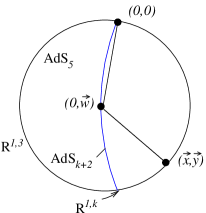
Figure 2.2: Witten diagram for bulk-defect two-point functions.

$\hat{{\cal O}}_{\hat{\Delta}}$

$K_{\hat{\Delta}}$

$K_{\Delta}$

${{\cal O}}_{\Delta}$

The two-point function $\langle{{\cal O}}_{\Delta}(\vec{x},\vec{y})\hat{{\cal O}}_{\hat{\Delta}}(0)\rangle$ is the integral over the product of the bulk-boundary propagators $K_{\Delta}\big{(}w,(\vec{x},\vec{y}),(\vec{0},\vec{w})\big{)}$ and $K_{\hat{\Delta}}\big{(}w,(\vec{0},\vec{w}),(\vec{0},\vec{0})\big{)}$,

$$\langle{{\cal O}}_{\Delta}(\vec{x},\vec{y})\hat{{\cal O}}_{\hat{\Delta}}(\vec{0})\rangle=\frac{\lambda^{(k-1)/4}}{N^{1/2}}\frac{\Gamma(\Delta)}{\pi^{2}\Gamma(\Delta-2)}\frac{\Gamma(\hat{\Delta})}{\pi^{(k+1)/2}\Gamma(\hat{\Delta}-\frac{k+1}{2})}J(\vec{x},\vec{y};\Delta,\hat{\Delta})$$ (2.43)

with the integral

$$J(\vec{x},\vec{y};\Delta,\hat{\Delta}) =\int\frac{dwd\vec{w}^{k+1}}{w^{k+2}}\left(\frac{w}{w^{2}+\vec{x}^{2}+(\vec{w}-\vec{y})^{2}}\right)^{\Delta}\left(\frac{w}{w^{2}+\vec{w}^{2}}\right)^{\hat{\Delta}}\,$$ (2.44)

$$=\frac{1}{(\vec{x}^{2}+\vec{y}^{2})^{\Delta}}\int dw^{\prime}d\vec{w}^{\prime k+1}\,w^{\prime\hat{\Delta}-(k+2)}\left(\frac{w^{\prime}}{w^{\prime 2}+\vec{x}^{\prime 2}+(\vec{w}^{\prime}-\vec{y}^{\prime})^{2}}\right)^{\Delta}\,.$$

In the last line we made use of the inversion trick [136] by defining

$$(w^{\prime},0,\vec{w}^{\prime})=\frac{1}{w^{2}+\vec{w}^{2}}(w,0,\vec{w}),\qquad(\vec{x}^{\prime},\vec{y}^{\prime})=\frac{1}{\vec{x}^{2}+\vec{y}^{2}}(\vec{x},\vec{y})\,.$$ (2.45)

The corresponding Witten diagram is shown in Fig. 2.2.

As in [61], we rescale $\vec{w}^{\prime}=\vec{y}^{\prime}+\sqrt{\vec{x}^{\prime 2}+w^{\prime 2}}\vec{v}$ and $w^{\prime}=|\vec{x}^{\prime}|u$ and find

$$J(\vec{x},\vec{y};\Delta,\hat{\Delta}) =\frac{1}{(\vec{x}^{2}+\vec{y}^{2})^{\hat{\Delta}}|\vec{x}|^{\Delta-\hat{\Delta}}}\int du\frac{u^{\hat{\Delta}-(k+2)+\Delta}}{(1+u^{2})^{\Delta-(k+1)/2}}\int d\vec{v}^{k+1}\frac{1}{(1+\vec{v}^{2})^{\Delta}}$$

$$=\frac{1}{(\vec{x}^{2}+\vec{y}^{2})^{\hat{\Delta}}|\vec{x}|^{\Delta-\hat{\Delta}}}\frac{\Gamma(\frac{\Delta-\hat{\Delta}}{2})\Gamma(\frac{\Delta+\hat{\Delta}}{2}-\frac{k+1}{2})}{2\Gamma(\Delta)}\,.$$ (2.46)

This converges if $\Delta>\hat{\Delta}$ and $\Delta+\hat{\Delta}>k+1$. The scaling $1/((\vec{x}^{2}+\vec{y}^{2})^{\hat{\Delta}}|\vec{x}|^{\Delta-\hat{\Delta}})$ agrees with the behaviour of the two-point function fixed by conformal invariance, cf. Eq. (A.21).

The defect-defect correlator $\langle\hat{{\cal O}}_{\hat{\Delta}}(\vec{y})\hat{{\cal O}}_{\hat{\Delta}}(\vec{0})\rangle$ for a defect operator $\hat{{\cal O}}_{\hat{\Delta}}$ is given by [136]

$$\langle\hat{{\cal O}}_{\hat{\Delta}}(\vec{y})\hat{{\cal O}}_{\hat{\Delta}}(\vec{0})\rangle=\eta\epsilon^{2(\hat{\Delta}-d)}\frac{2\hat{\Delta}-d}{\hat{\Delta}}\frac{\Gamma(\hat{\Delta}+1)}{\pi^{\frac{d}{2}}\Gamma(\hat{\Delta}-\frac{d}{2})}\frac{1}{|\vec{y}|^{2\hat{\Delta}}}$$ (2.47)

with $d=k+1$, which holds for $\hat{\Delta}>d/2$.

2.4 The conformal field theory of the D3-D3 brane intersection

Thus far we have only studied the defect CFT on the D3-D$p$ intersection with $p\in\{3,5,7\}$ in terms of its holographic dual, without ever writing the action. In the following we demonstrate the construction of its action specialising to $p=3$. We will find the low-energy effective action of $N$ D3-branes orthogonally intersecting $N^{\prime}$ D$3^{\prime}$-branes over two common dimensions. In the discussion of holography it was assumed that $N\rightarrow\infty$ with $\lambda=g_{YM}^{2}N$ and $N^{\prime}$ fixed, such that the open strings with both endpoints on the D3^′-brane decoupled. We will not make this assumption in constructing the action.

The ${\cal N}=4$ SYM $SU(N)$ theory located on the D3-branes and the ${\cal N}=4$ SYM $SU(N^{\prime})$ theory located on the D$3^{\prime}$-branes couple to a $(4,4)$ hypermultiplet at a two-dimensional defect. Although $(4,4)$ supersymmetry with $8$ supercharges is preserved, it is convenient to work with $(2,2)$ superspace. The world-volume of both stacks of D3-branes can be viewed as two ${\cal N}=2,d=4$ superspaces, intersecting over a two-dimensional $(2,2)$ superspace. One of the ${\cal N}=2,d=4$ superspaces is spanned by

$${\cal X}\sim(z^{+},z^{-},w,\bar{w},\theta_{(i)}^{\alpha},\bar{\theta}^{(i)}_{\dot{\alpha}})\,,$$ (2.48)

with $z^{\pm}=X^{0}\pm X^{1}$ and $w=X^{2}+iX^{3}$. The index $\alpha$ is a spinor index with values $1,2$, while the index $i$ accounts for the ${\cal N}=2$ supersymmetry and has values $1,2$. The other ${\cal N}=2,d=4$ superspace is spanned by

$${\cal X}^{\prime}\sim(z^{+},z^{-},y,\bar{y},\Theta_{(i)}^{\alpha},\bar{\Theta}^{(i)}_{\dot{\alpha}})\,,$$ (2.49)

where $y=X^{4}+iX^{5}$ and one makes the identification

$$\theta^{1}_{(1)}=\Theta^{1}_{(1)}\equiv\theta^{+}\,,$$ (2.50)

$$\theta^{2}_{(2)}=\Theta^{2}_{(2)}\equiv\bar{\theta}^{-}\,.$$ (2.51)

This is not the unique choice. For instance one could have written $\theta^{2}_{(2)}=\Theta^{2}_{(2)}\equiv\theta^{-}$ which is related to the first choice by mirror symmetry [137]. The intersection is the $(2,2),d=2$ superspace spanned by

$${\cal X}\cap{\cal X}^{\prime}\sim(z^{+},z^{-},\theta^{+},\theta^{-},\bar{\theta}^{+},\bar{\theta}^{-})\,.$$ (2.52)

All the degrees of freedom describing the D3-D3^′ intersection can be written in $(2,2)$ superspace. For instance the D3-D3 strings, which are not restricted to the intersection, can be described by $(2,2)$ superfields carrying extra (continuous) labels $w,\bar{w}$. Similiarly superfields associated to the D$3^{\prime}$-D$3^{\prime}$ strings carry the extra labels $y,\bar{y}$. Fields associated to D3-D$3^{\prime}$ strings are localized on the intersection and have no extra continuous labels.

Due to the breaking of four-dimensional supersymmetry by the couplings to the degrees of freedom localized at the intersection, it is convenient to write the action in a language in which the unbroken $(2,2)$ symmetry is manifest. This leads to a somewhat unusual form for the four-dimensional parts of the action. One way to obtain this action is somewhat akin to deconstruction [103]. The basic idea is to start with a conventional $(4,4)$ two-dimensional action in $(2,2)$ superspace, add an extra continuous label $w,\bar{w}$ to all the fields, and then try to add terms preserving $(4,4)$ supersymmetry such that there is a (non-manifest) four-dimensional Lorentz invariance. A four-dimensional Lorentz invariant theory which has a two-dimensional $(4,4)$ supersymmetry must also have ${\cal N}=4$ supersymmetry in four dimensions. The procedure of constructing a supersymmetric D-dimensional theory using a lower dimensional superspace has been employed in several contexts [138, 62, 139, 140]. The reader wishing to skip directly to the action of the D3-D3 intersection in $(2,2)$ superspace may proceed to Sec. 2.4.2.

2.4.1 Four-dimensional actions in lower dimensional superspaces

The approach of building four-dimensional Lorentz invariance starting with a conventional $(4,4)$ supersymmetric theory is an indirect but effective way to obtain the ${\cal N}=4,d=4$ super Yang-Mills action in a two-dimensional superspace. There is also a more direct approach which gives a $(2,2)$ superspace representation for the part of the ${\cal N}=4,d=4$ action containing only the ${\cal N}=2,d=4$ vector multiplet. The ${\cal N}=2,d=4$ vector multiplet has a straightforward decomposition under two-dimensional $(2,2)$ supersymmetry. On the other hand, there is no off-shell ${\cal N}=2,d=4$ formalism for the hypermultiplet, unless one uses harmonic superspace. We demonstrate the decomposition of the vector multiplet below. This provides a useful check of at least part of the action appearing in Sec. 2.4.2.

Embedding $(2,2)$, $d=2$ in ${\cal N}=2$, $d=4$

We begin by showing how to embed $(2,2)$, $d=2$ superspace into ${\cal N}=2$, $d=4$ superspace. The ${\cal N}=2,d=4$ superspace is parameterized by ($z^{+},z^{-},w,\bar{w}$, $\theta^{(i)}_{\alpha}$, $\bar{\theta}^{(i)}_{\dot{\alpha}}$). For the embedding let us redefine these coordinates as

$$\theta^{+} \equiv\theta_{(1)}^{1},\quad\theta\!\!\!/^{+}\equiv\theta_{(2)}^{1}\,,$$

$$\bar{\theta}^{-} \equiv\theta_{(2)}^{2},\quad\theta\!\!\!/^{-}\equiv\theta_{(1)}^{2}\,.$$ (2.53)

In the absence of central charges, the ${\cal N}=2$, $d=4$ supersymmetry algebra is

$$\{Q_{(i)\alpha},\bar{Q}^{(j)}{}_{\dot{\beta}}\} =2\rho^{\mu}_{\alpha\dot{\beta}}P_{\mu}\delta_{i}^{j},\qquad i,j=1,2\,,$$

$$\{Q_{(i)\alpha},Q_{(j)\beta}\} =\{\bar{Q}^{(i)}{}_{\dot{\alpha}},\bar{Q}^{(j)}{}_{\dot{\beta}}\}=0\,$$ (2.54)

with Pauli matrices $\rho^{\mu}$ given by Eq. (A.24). We define supersymmetry charges $Q_{+}\equiv Q_{(1)1}$, $\bar{Q}_{-}\equiv Q_{(2)2}$, $Q\!\!\!\!/\,_{+}\equiv Q_{(2)1}$, and ${{Q\!\!\!\!/\,_{-}}\equiv Q_{(1)2}}$. Following the methods of refs. [141, 142], we introduce a superspace defect at

$$w=0,\quad\theta\!\!\!/^{+}=\theta\!\!\!/^{-}=0\,,$$

which implies that the generators $P_{2}$, $P_{3}$, $Q\!\!\!\!/\,_{\pm}$, and $\bar{Q}\!\!\!\!/\,_{\pm}$ are broken. The unbroken subalgebra of (2.54) is generated by $Q_{\pm}$ and $\bar{Q}_{\pm}$ and turns out to be the $(2,2)$, $d=2$ supersymmetry algebra given by

$$\{Q_{\pm},\bar{Q}_{\pm}\}=2(P_{0}\pm P_{1})\,.$$ (2.55)

Other anticommutators of the $Q$’s vanish due to the absence of central charges.

${\cal N}=2$, $d=4$ Super Yang-Mills action in $(2,2)$, $d=2$ language

In order to derive the ${\cal N}=2$ Yang-Mills action in $(2,2)$ language, we decompose the four-dimensional ${\cal N}=2$ abelian vector superfield $\Psi$ in terms of a two-dimensional $(2,2)$ chiral superfield $\Phi$, a twisted chiral superfield $\Sigma$, and a vector superfield $V$. In the abelian case, the twisted chiral superfield (see e.g. Ref. [137, 143]) is related to the vector multiplet by

$$\Sigma\equiv\bar{D}_{+}D_{-}V$$ (2.56)

and satisfies $\bar{D}_{+}\Sigma=D_{-}\Sigma=0$. The $(2,2)$ vector and chiral superfields can be obtained by dimensional reduction of their ${\cal N}=1,d=4$ counterparts.

In App. A.6 we show that the ${\cal N}=2$, $d=4$ vector supermultiplet $\Psi$ decomposes into

$$\Psi=-i\Sigma+\theta\!\!\!/^{+}\bar{D}_{+}\left(\bar{\Phi}-\partial_{\bar{w}}V\right)+\theta\!\!\!/^{-}D_{-}\left(\Phi-\partial_{w}V\right)+\theta\!\!\!/^{+}\theta\!\!\!/^{-}G\,,$$ (2.57)

where $\partial_{w}$ is the transverse derivative and $G$ an auxiliary $(2,2)$ superfield. An interesting result of the decomposition is that the auxiliary field $D$ of the twisted chiral superfield $\Sigma$ is related to the component $D^{\prime}$ and transverse derivatives of the components $v^{\prime}_{2}$ and $v^{\prime}_{3}$ of the four-dimensional vector superfield,

$$D=\frac{1}{\sqrt{2}}\left(D^{\prime}+f^{\prime}_{32}\right)\,,$$ (2.58)

where $f^{\prime}_{32}=\partial_{3}v^{\prime}_{2}-\partial_{2}v^{\prime}_{3}$. Note that in distinction to the conformal field theory dual to the $(2|\rm D3\perp D5)$ intersection studied in [61, 62] there are no transverse derivatives like $\partial_{w}\phi^{\prime}$ in the auxiliary fields $F$ of the (2,2) superfield $\Phi$.

With the above decomposition of $\Psi$, we can now write down the ${\cal N}=2$, $d=4$ (abelian) Yang-Mills action in (2,2) language. Substituting Eq. (2.57) with $G=\bar{D}_{+}D_{-}(i\Sigma^{\dagger}+...)$ into the usual form of the YM action, we find

$$\frac{1}{4\pi}{\rm\,Im\,}\tau\int d^{4}xd^{2}\theta_{(1)}d^{2}\theta_{(2)}\,\frac{1}{2}\Psi^{2}$$ (2.59)

$$=\frac{1}{4\pi}{\rm\,Im\,}\tau\int d^{4}xd^{4}\theta\,\left(\bar{\Sigma}\Sigma+\bar{\Phi}\Phi+\partial_{\bar{w}}V\Phi-\bar{\Phi}\partial_{w}V-\partial_{\bar{w}}V\partial_{w}V\right),$$

with $d^{4}\theta=\frac{1}{4}d\theta^{+}d\theta^{-}d\bar{\theta}^{+}d\bar{\theta}^{-}$. From this one can easily deduce the corresponding non-abelian Yang-Mills action for vanishing $\theta$ angle,

$$S^{\rm nonab}_{\rm YM}=\frac{1}{g^{2}}\int d^{4}xd^{4}\theta{\rm\,tr}\left(\Sigma^{\dagger}\Sigma+(\partial_{\bar{w}}+\bar{\Phi})e^{V}(\partial_{w}+\Phi)e^{-V}\right)\,.$$ (2.60)

2.4.2 The D3-D3 action in $(2,2)$ superspace

We now present the full action for the $(4,4)$ supersymmetric theory describing the intersecting stacks of D3-branes. The action has the form

$$S=S_{\rm D3}+S_{\rm D3^{\prime}}+S_{\rm D3-D3^{\prime}}\,.$$ (2.61)

For each stack of parallel D3-branes we have separate actions, $S_{\rm D3}$ and $S_{\rm D3^{\prime}}$, each of which correspond to an ${\cal N}=4,d=4$ SYM theory with gauge groups $SU(N)$ and $SU(N^{\prime})$, respectively. The term $S_{\rm D3-D3^{\prime}}$ describes the coupling of these theories to matter on the two-dimensional intersection.

In $(2,2)$ superspace, the field content of $S_{\rm D3}$ is as follows. First, there is a vector multiplet $V(z^{\pm},\theta^{\pm},\bar{\theta}^{\pm};w,\bar{w})$ or, more precisely, a continuous set of vector multiplets labeled by $w,\bar{w}$ which are functions on the $(2,2)$ superspace spanned by $(z^{\pm},\theta^{\pm},\bar{\theta}^{\pm})$. The label $w=X^{2}+iX^{3}$ parameterizes the directions of the D3 world-volume transverse to the intersection, while $z^{\pm}=X^{0}\pm X^{1}$ parameterizes the remaining directions. Under gauge transformations $V$ transforms as

$$e^{V}\rightarrow e^{-i\Lambda^{\dagger}}e^{V}e^{i\Lambda}\,,\qquad e^{-V}\rightarrow e^{-i\Lambda}e^{-V}e^{i\Lambda^{\dagger}}\,,$$ (2.62)

where $\Lambda$ is a $(2,2)$ chiral superfield which also depends on $w,\bar{w}$. From $V$ one can build a twisted chiral (or field strength) multiplet as

$$\Sigma=\frac{1}{2}\{\bar{\cal D}_{+},{\cal D}_{-}\}\,,$$ (2.63)

where ${\cal D}_{\pm}=e^{-V}D_{\pm}e^{V}$, ${\cal\bar{D}}_{\pm}=e^{V}\bar{D}_{\pm}e^{-V}$. Additionally one has a pair of adjoint chirals $Q_{1}$ and $Q_{2}$, transforming as

$$Q_{i}\rightarrow e^{-i\Lambda}Q_{i}e^{i\Lambda}\,.$$ (2.64)

Finally there is a $(2,2)$ chiral field $\Phi$ which transforms such that $\partial_{\bar{w}}+\Phi$ is a covariant derivative:

$$\partial_{\bar{w}}+\Phi\rightarrow e^{-i\Lambda}(\partial_{\bar{w}}+\Phi)e^{i\Lambda}\,.$$ (2.65)

The complex scalar which is the lowest component of $\Phi$ is equivalent to the gauge connection $v_{2}+iv_{3}$ of the four-dimensional SYM theory described by $S_{\rm D3}$. This structure was also seen in the explicit decomposition of the ambient ${\cal N}=2$, $d=4$ vector field $\Psi$ under $(2,2),d=2$ supersymmetry discussed in Sec. 2.4.1, cf. Eq. (A.33).

The action of the second D3-brane (D$3^{\prime}$) is identical to that of the first D3-brane with the replacements

$$w\rightarrow y\,,\quad V\rightarrow{\cal V}\,,\quad\Sigma\rightarrow\Omega\,,\quad Q_{i}\rightarrow S_{i}\,,\quad\Phi\rightarrow\Upsilon\,,$$ (2.66)

and is invariant under gauge transformations $\Lambda^{\prime}$.

The fields corresponding to D3-D$3^{\prime}$ strings are the chiral multiplets $B$ and $\tilde{B}$, which are bifundamental and anti-bifundamental respectively with respect to $SU(N)\times SU(N^{\prime})$ gauge transformations;

$$B\rightarrow e^{-i\Lambda}Be^{i\Lambda^{\prime}}\,,\qquad\tilde{B}\rightarrow e^{-i\Lambda^{\prime}}\tilde{B}e^{i\Lambda}\,.$$ (2.67)

Using a canonical normalization ($V\rightarrow gV$ etc.), the components of the action are as follows:

$$S_{\rm D3}=\, \frac{1}{g^{2}}\int d^{2}zd^{2}wd^{4}\theta{\rm\,tr}\left(\Sigma^{\dagger}\Sigma+(\partial_{w}+g\bar{\Phi})e^{gV}(\partial_{\bar{w}}+g\Phi)e^{-gV}+\sum_{i=1,2}e^{-gV}\bar{Q}_{i}e^{gV}Q_{i}\right)$$

$$+ \int d^{2}zd^{2}wd^{2}\theta\epsilon_{ij}{\rm\,tr\,}Q_{i}[\partial_{\bar{w}}+g\Phi,Q_{j}]+c.c$$ (2.68)

$$S_{\rm D3^{\prime}}=\, \frac{1}{g^{2}}\int d^{2}zd^{2}yd^{4}\theta{\rm\,tr}\left(\Omega^{\dagger}\Omega+(\partial_{y}+g\bar{\Upsilon})e^{g{\cal V}}(\partial_{\bar{y}}+g\Upsilon)e^{-g{\cal V}}+\sum_{i=1,2}e^{-g{\cal V}}\bar{S}_{i}e^{g{\cal V}}S_{i}\right)$$

$$+ \int d^{2}zd^{2}yd^{2}\theta\epsilon_{ij}{\rm\,tr\,}S_{i}[\partial_{\bar{y}}+g\Upsilon,S_{j}]+c.c$$ (2.69)

$$S_{\rm D3-D3^{\prime}}= \int d^{2}zd^{4}\theta{\rm\,tr}\left(e^{-g\cal V}\bar{B}e^{gV}B+e^{-gV}\bar{\tilde{B}}e^{g\cal V}\tilde{B}\right)\hskip 156.49014pt$$

$$+ \frac{ig}{{2}}\int d^{2}zd^{2}\theta{\,\rm tr}\left(B\tilde{B}Q_{1}-\tilde{B}BS_{1}\right)+c.c.$$ (2.70)

with $d^{4}\theta=\frac{1}{4}d\theta^{+}d\theta^{-}d\bar{\theta}^{+}d\bar{\theta}^{-}$ and $d^{2}\theta=\frac{1}{2}d\theta^{+}d\theta^{-}$.

Some comments about $S_{\rm D3}$ are in order. We have already presented part of this action, as the first two terms in the $S_{\rm D3}$ are given by Eq. (2.60). Upon integrating out auxiliary fields, $S_{\rm D3}$ can be seen to describe the ${\cal N}=4$ SYM theory. To illustrate how four-dimensional Lorentz invariance arises, consider the superpotential $\epsilon_{ij}{\rm\,tr\,}Q_{i}[\partial_{\bar{w}}+\Phi,Q_{j}]$. Upon integrating out the F-terms of $Q_{1}$ and $Q_{2}$, one gets kinetic terms in the $X^{2},X^{3}$ directions which are the four-dimensional Lorentz completion of the kinetic terms in the $X^{0},X^{1}$ directions arising from $e^{-V}\bar{Q}_{i}e^{V}Q_{i}$.

The form of $S_{\rm D3-D3^{\prime}}$ is dictated by gauge invariance and $(4,4)$ supersymmetry. The geometric interpretation of various fields can be seen from this part of the action. The vacuum expectation values for the scalar components of $Q_{1}$ and $S_{1}$ give rise to mass terms for the fields $B$ and $\tilde{B}$ localized at the intersection. There are also “twisted” mass terms for $B$ and $\tilde{B}$ which arise when the scalar components of the twisted chiral fields $\Sigma$ and $\Omega$ (or equivalently of $V$ and ${\cal V}$) get expectation values. One expects $B$ and $\tilde{B}$ fields to become massive when the D3-branes are separated from the D3^′-branes in the $X^{6,7,8,9}$ directions transverse to both. Thus we associate the scalar components of $(Q_{1},\Sigma)$ or $(S_{1},\Omega)$ with fluctuations in $(X^{6}+iX^{7},X^{8}+iX^{9})$.

Note that in $(2,2)$ superspace, $Q_{2}$ and $S_{2}$ are not directly coupled to the fields $B$ and $\tilde{B}$, although derivative couplings arise after integrating out the F-terms of $Q_{1}$ and $S_{1}$. The scalar component of $Q_{2}$ describes fluctuations of the D3-branes in the $y=X^{4}+iX^{5}$ plane parallel to the D3^′-branes. Similiarly the scalar components of $S_{2}$ describe fluctuations of the D3^′-branes in the $w=X^{2}+iX^{3}$ plane parallel to the D3-branes.

2.4.3 R-symmetries

The isometries of the AdS background are $SL(2,R)\times SL(2,R)\times U(1)\times SU(2)_{L}\times SU(2)_{R}\times U(1)$, as can be seen from Eq. (2.9) for $k=1$. The $SU(2)_{L}\times SU(2)_{R}$ component is an R-symmetry which acts as rotations in the $6,7,8$ and $9$ directions transverse to all the D3-branes. The first $U(1)$ R-symmetry acts as a rotation in the $w$ (or $23$) plane, while the second $U(1)$ acts as a rotation in the $y$ (or $45$) plane. In the near horizon geometry, the probe Kaluza-Klein momentum on $S^{1}$ is a contribution to $J_{45}$. The charge $J_{23}$ generates a rotation in $AdS_{5}$ directions orthogonal to the probe.

Below we summarize the R-charges and engineering dimensions of the fields of the D3-D3 intersection.

(4,4)	(2,2)	components	$(j_{L},j_{R})$	$J_{23}$	$J_{45}$	$\Delta$
		$\sigma,q_{1}$	$(\frac{1}{2},\frac{1}{2})$	$0$	$0$	$1$
Vector	$Q_{1},\Sigma$	$\psi_{q_{1}}^{+},\bar{\lambda}_{\sigma}^{+}$	$(0,\frac{1}{2})$	$\frac{1}{2}$	$-\frac{1}{2}$	$\frac{3}{2}$
		$\psi_{q_{1}}^{-},\bar{\lambda}_{\sigma}^{-}$	$(\frac{1}{2},0)$	$\frac{1}{2}$	$-\frac{1}{2}$	$\frac{3}{2}$
		$v_{0},v_{1}$	$(0,0)$	$0$	$0$	$1$
		$\phi$	$(0,0)$	$-1$	$0$	$1$
Hyper	$Q_{2},\Phi$	$q_{2}$	$(0,0)$	$0$	$1$	$1$
		$\psi_{\phi}^{+},\bar{\psi}_{q_{2}}^{+}$	$(\frac{1}{2},0)$	$-\frac{1}{2}$	$-\frac{1}{2}$	$\frac{3}{2}$
		$\psi_{\phi}^{-},\bar{\psi}_{q_{2}}^{-}$	$(0,\frac{1}{2})$	$-\frac{1}{2}$	$-\frac{1}{2}$	$\frac{3}{2}$
		$b$	$(0,0)$	$-\frac{1}{2}$	$\frac{1}{2}$	0
Hyper	$B,\tilde{B}$	$\tilde{b}$	$(0,0)$	$-\frac{1}{2}$	$\frac{1}{2}$	$0$
		$\psi_{b}^{+},\bar{\psi}_{\tilde{b}}^{+}$	$(\frac{1}{2},0)$	$0$	$0$	$\frac{1}{2}$
		$\psi_{b}^{-},\bar{\psi}_{\tilde{b}}^{-}$	$(0,\frac{1}{2})$	$0$	$0$	$\frac{1}{2}$
		$\omega,s_{1}$	$(\frac{1}{2},\frac{1}{2})$	$0$	$0$	$1$
Vector	$S_{1},\Omega$	$\psi_{s_{1}}^{+},\bar{\psi}_{\omega}^{+}$	$(0,\frac{1}{2})$	$\frac{1}{2}$	$-\frac{1}{2}$	$\frac{3}{2}$
		$\psi_{s_{1}}^{-},\bar{\psi}_{\omega}^{-}$	$(\frac{1}{2},0)$	$\frac{1}{2}$	$-\frac{1}{2}$	$\frac{3}{2}$
		$\tilde{v}_{0},\tilde{v}_{1}$	$(0,0)$	$0$	$0$	$1$
		$\upsilon$	$(0,0)$	$0$	$1$	1
Hyper	$S_{2},\Upsilon$	$s_{2}$	$(0,0)$	$-1$	$0$	$1$
		$\lambda_{\upsilon}^{+},\bar{\psi}_{s_{2}}^{+}$	$(\frac{1}{2},0)$	$\frac{1}{2}$	$\frac{1}{2}$	$\frac{3}{2}$
		$\lambda_{\upsilon}^{-},\bar{\psi}_{s_{2}}^{-}$	$(0,\frac{1}{2})$	$\frac{1}{2}$	$\frac{1}{2}$	$\frac{3}{2}$

Table 2.2: Field content of the D3-D3 intersection.

The $U(1)$ symmetries generated by $J_{45}$ and $J_{23}$ are manifest in $(2,2)$ superspace. The $U(1)$ generated by $J_{45}$ has the following action:

$$\theta^{+}\rightarrow e^{i\alpha/2}\theta^{+}\,, B\rightarrow e^{i\alpha/2}B\,, Q_{2}\rightarrow e^{i\alpha}Q_{2}\,,$$

$$\theta^{-}\rightarrow e^{i\alpha/2}\theta^{-}\,, \tilde{B}\rightarrow e^{i\alpha/2}\tilde{B}\,, \Upsilon\rightarrow e^{+i\alpha}\Upsilon\,,$$

$$y\rightarrow e^{i\alpha}y\,,$$ (2.71)

with all remaining fields being singlets. The $U(1)$ generated by $J_{23}$ acts as

$$\theta^{+}\rightarrow e^{-i\alpha/2}\theta^{+}\,, B\rightarrow e^{-i\alpha/2}B\,, S_{2}\rightarrow e^{-i\alpha}S_{2}\,,$$

$$\theta^{-}\rightarrow e^{-i\alpha/2}\theta^{-}\,, \tilde{B}\rightarrow e^{-i\alpha/2}\tilde{B}\,, \Phi\rightarrow e^{-i\alpha}\Phi\,,$$

$$w\rightarrow e^{-i\alpha}w\,.$$ (2.72)

The reader may be surprised that these R-symmetries act on the coordinates $w$ and $y$. However in the language of two-dimensional superspace, these are continuous labels rather than space-time coordinates. Recall also that $J_{23}$ (or $J_{45}$) is an R-symmetry of the ${\cal N}=4$ algebra associated with one stack of D3-branes, but a Lorentz symmetry for the orthogonal stack.

2.4.4 Quantum conformal invariance

Here we give an argument that the action given by (2.4.2), (2.69) and (2.70) does not receive quantum corrections, such that it remains conformal to all orders in perturbation theory. We will not attempt a rigorous proof here, but we give an argument for conformal invariance using our $(2,2)$, $d=2$ formulation of the model. The argument relies on the assumption that the classical $(2,2)$, $d=2$ supersymmetry is unbroken by quantum corrections. This argument is analogous to the discussion of the 3d/4d case in [62], where more details on the renormalization procedure may be found.

The argument for excluding possible quantum breakings of conformal symmetry by defect operators relies on considering the $(2,2)$ supercurrent and its possible anomalies, and by making the assumption that $(4,4)$ supersymmetry is preserved by the quantum corrections.

We begin by recalling the situation in ${\cal N}=1$, $d=4$ theories, see for instance [145]. In this case there is a supermultiplet $J_{\dot{\alpha}\beta}=\sigma^{\mu}{}_{\dot{\alpha}\beta}J_{\mu}$, which has the R-current $R_{\mu}$ (sometimes also denoted as $j_{\mu}^{(5)}$), the supersymmetry currents $Q_{\mu\alpha}$ and the energy-momentum tensor $T_{\mu\nu}$ among its components. These are the Noether currents corresponding to R transformations, supersymmetry transformations and translations. The supermultiplet $J_{\mu}$ can be expanded as

$$J_{\mu}(x,\theta,\bar{\theta})=R_{\mu}(x)-i\theta^{\alpha}Q_{\mu\alpha}(x)+\bar{\theta}_{\dot{\alpha}}\bar{Q}_{\mu}^{\dot{\alpha}}(x)-2(\theta\sigma^{\nu}\bar{\theta})T_{\mu\nu}(x)+...$$ (2.73)

Potential superconformal anomalies may be written in the form

$$\bar{D}^{\dot{\alpha}}J_{\dot{\alpha}\beta}\,=\,D_{\beta}S\,,$$ (2.74)

with $S$ a chiral superfield. When $S=0$, superconformal symmetry is conserved. In ${\cal N}=1$, $d=4$ the superfield $S$ is proportional to the operator $W_{\alpha}W^{\alpha}$. When written in components, Eq. (2.74) contains both the trace anomaly and the anomalous divergences of the R-symmetry and supersymmetry currents.

By standard dimensional reduction to $(2,2)$ supersymmetry in two dimensions, we obtain from (2.74), as shown in [146],

$$(\gamma^{M})_{A}{}^{B}\bar{D}_{B}{\cal J}_{M}\,=D_{A}\,{\cal S}\,,$$ (2.75)

where $M=\{1,2\}$, $A,B=\{+,-\}$, $\gamma^{M}=\{\sigma^{1},i\sigma^{2}\}$ are the two-dimensional gamma matrices, ${\cal J}_{M}$ is the two-dimensional $(2,2)$ supercurrent and the possible conformal anomaly is given by the $(2,2)$ chiral superfield ${\cal S}$. ${\cal J}_{M}$ contains the 2d R-current, the four $(2,2)$ supersymmetry currents and the 2d energy-momentum tensor.

For 2d/4d models like the one given by (2.4.2), (2.69) and (2.70), the classically conserved two-dimensional supercurrent is given by

$${\cal J}_{M}(z)\,=\,{\cal J}^{\rm def}_{M}(z)\,+\,\int\!d^{2}w\;{\cal J}^{\rm bulk,1}_{M}(w,z)\,+\,\int\!d^{2}y\;{\cal J}^{\rm bulk,2}_{M}(y,z)\,.$$ (2.76)

Let us first consider possible defect operator contributions to the anomaly ${\cal S}$, which have to be gauge invariant and of dimension 1. The possible defect contributions to the anomaly ${\cal S}$ are given by

$${\cal S}_{D}\,=\,{\rm Tr}\,[u\,\bar{D}^{+}\bar{D}^{-}(e^{-\cal V}\bar{B}e^{V}B+e^{-V}\bar{\tilde{B}}e^{\cal V}\tilde{B})\,+\,\,v\,(B\tilde{B}Q_{1}-\tilde{B}BS_{1})\,]\,.$$ (2.77)

It is important to note that there is no gauge anomaly term contributing to this equation, since ${\rm Tr\,}\Sigma$ or ${\rm Tr\,}\Omega$, which would have the right dimension, are twisted chiral and not chiral. $u$ and $v$ are coefficients which may be calculated perturbatively. They are related to the $\beta$ and $\gamma$ functions. From the standard supersymmetric non-renormalization theorem we know that $v=0$ since the corresponding operator is chiral. $u$ may be non-zero in a general $(2,2)$ supersymmetric gauge theory. However $u$ and $v$ are related by $(4,4)$ supersymmetry. Therefore if we assume that $(4,4)$ supersymmetry is preserved upon quantization, $v=0$ also implies $u=0$. Thus there are no defect contributions breaking conformal symmetry.

We may also show that there are no contributions from four-dimensional operators to the conformal anomaly ${\cal S}$. Such terms would have to originate from bulk action counterterms. Consider correlation functions of bulk fields in the limit of large $|w|$ (or $|y|$) but fixed momenta $\vec{p}$ parallel to the defect. These receive the usual contributions from diagrams involving only bulk fields. Such contributions are finite due to the finiteness of the ${\cal N}=4$, $d=4$ theory. Contributions from diagrams which involve bulk-defect interactions (see Fig. 2.3) are $w$ (or $y$) dependent and fall off with distance from the defect. Therefore local counterterms generating the anomalies would be of the form

$${\cal S}_{B}\,\sim\,\int\!d^{2}w\,|w|^{-s_{1}}\Lambda^{t_{1}}{\cal O}_{1}(w,z)\,+\,\int\!d^{2}y\,|y|^{-s_{2}}\Lambda^{t_{2}}\,{\cal O}_{2}(y,z)\,,$$ (2.78)

with $\Lambda$ a regulator scale, and $s_{i}\geq 2$, $t_{i}\geq 0$ for $i=1,2$. However there are no such operators available in the theory. From dimensional analysis, only ${\rm Tr\,}\Sigma$ or ${\rm Tr\,}\Omega$ would be possible for ${\cal O}_{1}$ or ${\cal O}_{2}$, respectively, but again these are twisted chiral and not chiral. Therefore we conclude that there a no terms breaking $SO(2,2)$ conformal invariance, such that the theory is conformal to all orders in perturbation theory.

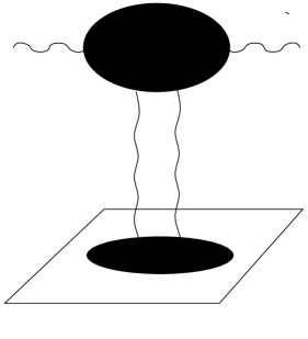
Figure 2.3: A $w$ dependent contribution to a bulk-bulk propagator.

$(|w|,\vec{p})$                         $(|w|,\vec{p})$

2d defect

2.5 More on the D3-D3 intersection

In this section we consider some interesting properties of the D3-D3 intersection which do not arise for the D3-D5 or the D3-D7 brane configuration. Most of the pecularities are due to the two-dimensional conformal symmetry preserved by the defect which differs in many aspects from conformal invariance in higher dimensions. A natural question to ask is whether the theory satisfies an infinite-dimensional Virasoro algebra. We will see however that only the finite part of the $(4,4)$ superconformal algebra, whose even part is $SL(2,R)\times SL(2,R)$, is realised in an obvious way. Roughly speaking, the $(4,4)$ superconformal algebra is the common intersection of two ${\cal N}=4,d=4$ superconformal algebras, both of which are finite. Enhancement to the usual infinite-dimensional algebra would require the existence of a decoupled two-dimensional sector which does not exist.

We then give a detailed dictionary between Kaluza-Klein fluctuations on the probe D3-brane and operators localized on the defect. Of particular interest will be a certain subset of the fluctuations which describe the embedding of the probe inside $AdS_{5}$. This subset is dual to operators containing defect scalar fields, which appear without any derivative or vertex operator structure. Due to strong infrared effects in two dimensions, these fields are not conformal fields associated to states in the Hilbert space. From the point of view of the probe-supergravity system, there is at first sight nothing unusual about these fluctuations. However upon applying the usual $AdS_{3}$/CFT₂ rules, we will find that the dual two-point correlator does not show a power law behaviour. Thus there is no clear interpretation of these fluctuations as sources for the generating function of the CFT. We shall find however that the bottom of the Kaluza-Klein tower for these fluctuations (with appropriate boundary conditions) parameterizes the holomorphic embedding $wy\sim c\alpha^{\prime}$ of the $AdS_{3}$ probe inside $AdS_{5}$ which we discussed in the last section. While the interpretation of this fluctuation as a source is unclear, it nevertheless labels points on the classical Higgs branch.

We finally compute perturbative quantum corrections to the two-point function of the BPS primary operators and find that such corrections are absent at order $g_{YM}^{2}$. In Sec. 2.3 we have seen in an AdS computation that correlation functions are independent of the ’t Hooft coupling. Both results suggest the existence of a non-renormalization theorem.

2.5.1 The $(4,4)$ superconformal algebra

The D3-D3 intersection has a $(4,4)$ superconformal group whose even part is

$$SL(2,R)\times SL(2,R)\times SU(2)_{L}\times SU(2)_{R}\times U(1)\,.$$ (2.79)

A comparison with the isometry group given by Eq. (2.9) for $k=1$, $SO(2,2)\times SO(2)\times SO(4)\times SO(2)$, shows that only a certain combination of the two $U(1)\simeq SO(2)$ factors enters the superconformal algebra. We emphasize that this system does not give a standard $(4,4)$ superconformal algebra. Because of the couplings between two and four-dimensional fields, the algebra does not factorize into left and right moving parts. Neither an infinite Virasoro algebra nor an affine Kac-Moody algebra are realised in any obvious way. The superconformal algebra for the D3-D3 system should be thought of as a common “intersection” of two ${\cal N}=4,d=4$ superconformal algebras, both of which are finite. If there is a hidden affine algebra, it should arise via some dynamics which gives a decoupled two-dimensional sector, for which we presently have no evidence.

For comparative purposes, it is helpful to first review the situation for more familiar two-dimensional $(4,4)$ theories with vector multiplets and hypermultiplets, such as those considered in [147]. These theories may have classical Higgs and Coulomb branches which meet at a singularity of the moduli space. For finite coupling, quantum states spread out over both the Higgs and Coulomb branches. However in the infrared (or strong coupling) limit, one obtains a separate $(4,4)$ CFT on the Higgs and Coulomb branches [147]. One argument for the decoupling of the Higgs and Coulomb branches is that the $(4,4)$ superconformal algebra contains an $SU(2)_{l}\times SU(2)_{r}$ R-symmetry with a different origin in the original $SU(2)_{L}\times SU(2)_{R}\times SU(2)$ R-symmetry depending on whether one is on the Higgs branch or Coulomb branch. The CFT scalars must be uncharged under the R-symmetries. This means for example that the original $SU(2)_{L}\times SU(2)_{R}$ factor may be the R-symmetry of the CFT on the Higgs branch but not the Coulomb branch.

For the linear sigma model describing the D3-D3 intersection, a $(4,4)$ super-conformal theory arises only on the Higgs branch, which is parameterized by the two-dimensional scalars of the defect hypermultiplet. On the Coulomb branch, the orthogonal D3-branes are separated by amounts characterised by the VEV’s of four-dimensional scalar fields. One obtains a CFT on the Higgs branch without flowing to the IR, since the gauge fields propagate in four dimensions and the gauge coupling is exactly marginal. Furthermore scalar degrees of freedom of the CFT may carry R-charges, since the R-currents do not break up into purely left and right moving parts. Of course the scalars of the defect hypermultiplet must still be uncharged under the R-symmetries, since for $g_{YM}=0$ the free $(4,4)$ hypermultiplet realises a conventional two-dimensional $(4,4)$ CFT. However the four-dimensional scalar fields, which are not decoupled at finite $g_{YM}$, transform non-trivially under the R-symmetries of the defect CFT.

In more familiar considerations of the $AdS_{3}/CFT_{2}$ duality, the full Virasoro algebra is realised in terms of diffeomorphisms that leave the form of the metric invariant asymptotically, near the boundary of $AdS_{3}$ [71]. Of these diffeomorphisms, the finite $SL(2,R)\times SL(2,R)$ subalgebra is realised as an exact isometry. However the three-dimensional diffeomorphisms which are asymptotic isometries of $AdS_{3}$, and correspond to higher-order Virasoro generators, do not have an extension into the bulk which leave the $AdS_{5}$ metric asymptotically invariant. The existence of a Virasoro algebra seems to require localized gravity on $AdS_{3}$. This could only be seen through a consideration of the back-reaction. Note also that a necessary condition for the existence of a Virasoro algebra is the existence of a two-dimensional conserved local energy-momentum tensor. This requirement is not satisfied as shown in App. A.4. In the defect CFT, the two-dimensional conformal algebra contains only those generators which can be extended to conformal transformations of the four-dimensional parts of the world-volume, namely $L_{-1},L_{0},L_{1},\tilde{L}_{-1},\tilde{L}_{0}$ and $\tilde{L}_{1}$.

The ‘global’ $(4,4)$ superconformal algebra of defect CFT gives relations between the dimensions and R-charges of BPS operators. We will later find that these relations are consistent with the spectrum of fluctuations in the probe-$AdS$ background. To construct the relevant part of the algebra, it is helpful to note that the algebra should be a subgroup of an ${\cal N}=4,d=4$ superconformal algebra (or actually an unbroken intersection of two such algebras).

Let us start by writing down the relevant part of the ${\cal N}=4,d=4$ superconformal algebra for the D3-branes in the $0123$ directions. The supersymmetry generators are $Q_{\alpha}^{a}$, where $\alpha=1,2$ is a spinor index and $a=1,\cdots,4$ is an index in the representation ${\bf 4}$ of the $SU(4)$ R-symmetry. The special superconformal generators are $S_{\beta b}$ which are in the ${\bf 4}^{*}$ representation of $SU(4)$. The relevant part of the ${\cal N}=4,d=4$ algebra is then

$$\{Q^{a}_{\alpha},S_{\beta b}\}=\epsilon_{\alpha\beta}({\delta_{b}}^{a}D+4J^{A}(T_{A})^{a}_{b})+\frac{1}{2}{\delta_{b}}^{a}L_{\mu\nu}\sigma^{\mu\nu}_{\alpha\beta}\,,$$ (2.80)

where $D$ is the dilation operator, $J^{A}$ are the operators generating $SU(4)$, and $L_{\mu\nu}$ are the generators of four-dimensional Lorentz transformations. The matrices $(T_{A})^{a}_{b}$ generate the fundamental representation of $SU(4)$, and are normalized such that ${\rm Tr}(T^{A}T^{B})=\frac{1}{2}\delta^{AB}$.

A $(4,4)$ supersymmetry sub-algebra is generated by the supercharges $Q^{a}_{1}\equiv Q^{a}_{+}$ with $a=1,2$, and $Q^{a}_{2}\equiv Q^{a}_{-}$ with $a=3,4$, on which an $SU(2)_{L}\times SU(2)_{R}\times U(1)$ subgroup of the orginal $SU(4)$ R-symmetry acts. The embedding of the $SU(2)_{L}\times SU(2)_{R}\times U(1)$ generators in $SU(4)$ is as follows:

$$SU(2)_{L}:\begin{pmatrix}\frac{1}{2}\sigma^{A}&0\cr 0&0\end{pmatrix},\quad SU(2)_{R}:\begin{pmatrix}0&0\cr 0&\frac{1}{2}\sigma^{B}\end{pmatrix},\quad U(1):\frac{1}{\sqrt{8}}\begin{pmatrix}-I&0\cr 0&I\end{pmatrix}\,.$$ (2.81)

The unbroken $SU(2)_{L}\times SU(2)_{R}$ R-symmetry corresponds to rotations in the directions $6,7,8,9$ transverse to both stacks of D3-branes, while the unbroken $U(1)$ describes rotation in the $45$ plane. These symmetries act on adjoint scalars. Since the R-currents of the CFT do not break up into left and right moving parts, there is no requirement that four-dimensional scalars are uncharged under R-symmetries. We shall call the generator of rotations in the $45$ plane $J_{45}$, and normalize it such that the supercharges $Q^{a}_{\pm}$ have $J_{45}$ eigenvalue $\pm 1/2$. The special superconformal generators of the $(4,4)$ sub-algebra are $S_{b2}\equiv S_{b-}$ with $b=1,2$ and $S_{b1}\equiv S_{b+}$ with $b=3,4$. The term in the $(4,4)$ algebra inherited from (2.80) is then

$$\{Q^{a}_{+},S_{b-}\} ={\delta_{b}}^{a}D+2J^{L}_{A}(\sigma^{A})^{a}_{b}+\delta^{a}_{b}J_{45}+\delta^{a}_{b}L_{01}+\delta^{a}_{b}L_{23}\,,$$ (2.82)

$$\{Q^{a}_{-},S_{b+}\} =-\delta_{b}^{a}D-2J^{R}_{A}(\sigma^{A})^{a}_{b}+\delta^{a}_{b}J_{45}+\delta^{a}_{b}L_{01}+\delta^{a}_{b}L_{23}\,.$$ (2.83)

The unbroken Lorentz generators are $L_{01}$ and $L_{23}$. Note that from a two-dimensional point of view, the Lorentz transformations are generated by $L_{01}$, whereas $L_{23}$ is an R-symmetry.

For the orthogonal D3-branes spanning $0,1,4,5$, rotations in the $45$ plane are Lorentz generators $L_{45}$ rather than a subgroup of $SU(4)$. The rotations in the $23$ plane are an unbroken $U(1)$ part of the $SU(4)$ R-symmetry rather than a Lorentz transformation. This distinction is illustrated in Fig. 2.4.

Figure 2.4: Decomposition of the two $SU(4)$ R-symmetries.

From the two-dimensional point of view, both $23$ and $45$ rotations are $U(1)$ R-symmetries. If we write $L_{23}=J_{23},\,L_{45}=J_{45}$ and define ${\cal J}=J_{23}+J_{45}$, then the terms (2.82) and (2.83) become

$$\{Q^{a}_{+},S_{b-}\} ={\delta_{b}}^{a}(L_{01}+D)+2J^{L}_{A}(\sigma^{A})^{a}_{b}+\delta^{a}_{b}{\cal J}\,,$$ (2.84)

$$\{Q^{a}_{-},S_{b+}\} =\delta_{b}^{a}(L_{01}-D)-2J^{R}_{A}(\sigma^{A})^{a}_{b}+\delta^{a}_{b}{\cal J}\,.$$ (2.85)

which are applicable to both stacks of D3-branes. This forms part of the $(4,4)$ superconformal algebra of the full D3-D3 system. The charge ${\cal J}$ plays a somewhat unusual role. From the point of view of the bulk four-dimensional fields, ${\cal J}$ is a combination of an R-symmetry and a Lorentz symmetry, under which the preserved supercharges are invariant. As we will see later, the fields localized at the two-dimensional intersection are not charged under ${\cal J}$. Upon decoupling the four-dimensional fields by taking $g=0$, the two-dimensional sector becomes a free $(4,4)$ superconformal theory with an affine $SU(2)_{L}\times SU(2)_{R}$ R-symmetry. However, for $g_{YM}\neq 0$, the algebra does not factorize into left and right moving parts.

The algebra (2.84, 2.85) determines the dimensions of the BPS superconformal primary operators, which are annihilated by all the $S$’s and some of the $Q$’s. The bounds on dimensions due to the superconformal algebra are best obtained in Euclidean space. The Euclidean $(4,4)$ algebra of the defect CFT contains the terms

$$\{{\cal Q}^{a}_{1/2},{\cal Q}_{1/2}^{b\dagger}\}=2\delta^{a}_{b}L_{0}+2J^{L}_{A}({\sigma^{A}})^{a}_{b}+\delta^{a}_{b}{\cal J}\,,$$ (2.86)

$$\{\tilde{\cal Q}^{a}_{1/2},\tilde{\cal Q}_{1/2}^{b\dagger}\}=2\delta^{a}_{b}\tilde{L}_{0}+2J^{R}_{A}({\sigma^{A}})^{a}_{b}-\delta^{a}_{b}{\cal J}\,.$$ (2.87)

For $a=b$, the left hand side of (2.86) and (2.87) are positive operators, leading to the bounds

$$h+j^{L}_{3}+\textstyle\frac{1}{2}{\cal J}\geq 0\,,$$ (2.88)

$$h-j^{L}_{3}+\textstyle\frac{1}{2}{\cal J}\geq 0\,,$$ (2.89)

$$\tilde{h}+j^{R}_{3}-\textstyle\frac{1}{2}{\cal J}\geq 0\,,$$ (2.90)

$$\tilde{h}-j^{R}_{3}-\textstyle\frac{1}{2}{\cal J}\geq 0\,,$$ (2.91)

some of which are saturated by the BPS super-conformal primaries. As always, the dimensions are $\Delta=h+\tilde{h}$, with $h=\tilde{h}$ for scalar operators.

2.5.2 Fluctuation–operator dictionary

In the following we find the map between fluctuations on the probe D3-brane and operators localized at the defect. The single particle states on the probe correspond to meson-like operators with strings of adjoint fields sandwiched between pairs of defect fields in the fundamental representation. The fluctuations can be devided into three classes: $S^{1}$ fluctuations, gauge field fluctuations, and $AdS_{3}$ fluctuations. These fluctuations follow from the analysis in Sec. 2.2 for $k=1$.

$S^{1}$ fluctuations inside $S^{5}$

The fluctuations of the probe $S^{1}$ embedding inside $S^{5}$ are characterised by the mode $V^{m}_{l}$ where $m=6,7,8,9$. As shown in Sec. 2.2.2 these fluctuations are scalars in the $(\frac{1}{2},\frac{1}{2})$ (vector) representation of $SO(4)\simeq SU(2)_{L}\times SU(2)_{R}$. Moreover, these fluctuations have $J_{23}=0$ and $J_{45}=l$ such that the $U(1)$ charge appearing in the algebra (2.86), (2.87) is ${\cal J}=l$. The possible series of dimensions are $\Delta=1\pm l$. We need only consider $l\geq 0$ since ${V^{m}_{l}}^{*}=V^{m}_{-l}$. In this case the sensible series of dimensions is $\Delta=1+l$. The only gauge invariant defect operator consistent with this is

$${\cal C}^{\mu l}\equiv\sigma^{\mu}_{ij}\left(\epsilon_{ik}\bar{\Psi}^{+}_{k}q_{2}^{l}\Psi^{-}_{j}+\epsilon_{jk}\bar{\Psi}^{-}_{k}q_{2}^{l}\Psi^{+}_{i}\right)\qquad(\mu=0,...,3)$$ (2.92)

where $\Psi^{+}_{i}$ and $\Psi^{-}_{i}$ are $SU(2)_{L}$ and $SU(2)_{R}$ doublets respectively, given by

$$\Psi^{+}_{i}=\begin{pmatrix}\psi_{b}^{+}\cr\bar{\psi}_{\tilde{b}}^{+}\end{pmatrix}\qquad\Psi^{-}_{i}=\begin{pmatrix}\psi_{b}^{-}\cr\bar{\psi}_{\tilde{b}}^{-}\end{pmatrix}\,.$$ (2.93)

The index $\mu$ is an $SO(4)$ index and should not be confused with a spacetime Lorentz index. Note that (2.92) is invariant under parity, which exchanges the $SU(2)_{L}$ index $i$ with the $SU(2)_{R}$ index $j$, as well as $+$ with $-$. This operator saturates the bound (2.91), i.e. only one of the bounds in (2.88)-(2.91), so it is actually $1/4$ BPS. For $l=0$, the operator is a pure defect operator which satisfies both the bounds (2.89) and (2.91) and thus is $1/2$ BPS. This operator will be shown to satisfy a non-renormalization theorem to order $g^{2}$ in Sec. 2.5.5.

Gauge field fluctuations

The gauge field fluctuations as derived in Sec. 2.2.3 transform trivially under $SU(2)_{L}\times SU(2)_{R}$ and have $J_{23}=0$ and $J_{45}=l$. If we pick the positive branch, the dimension of this operator is $\Delta=l+1$. On the field theory side, the operator at the bottom of the tower with the same quantum numbers is the current associated with a global $U(1)_{B}$ under which the defect fields transform,

$${\cal J}^{M}_{B}\equiv\bar{\Psi}^{\alpha}_{i}\rho^{M}_{\alpha\beta}\Psi_{i}^{\beta}+i\bar{b}\overleftrightarrow{D}^{M}b+i\tilde{b}\overleftrightarrow{D}^{M}\bar{\tilde{b}}\qquad(M=0,1)\,,$$ (2.94)

with Pauli matrices $\rho^{M}$ defined by Eq. (A.24), $\Psi$ as in (2.93), and $\alpha,\beta\in\left\{+,-\right\}$. Although this current is conserved and satisfies the BPS bound of the superconformal algebra, it is not a quasi-primary of the $SO(2,2)$ global conformal symmetry. This is essentially due to the fact that it is in the same (short) supersymmetry multiplet as the dimensionless field $\bar{b}b+\tilde{b}\bar{\tilde{b}}$.

The contributions to (2.94) involving $b$, $\tilde{b}$ lead to logarithms in the correlation functions. These are actually present even in the purely two-dimensional free field theory obtained by setting $g=0$ and thus decoupling the 2d from the 4d theory. In this case we have a bosonic current contribution of the form

$$J_{M}^{\rm 2d}=i\bar{b}\partial_{M}b-i(\partial_{M}\bar{b})b\,,$$ (2.95)

which is conserved. For Euclidean signature, this current has a correlator of the form

$$\langle J_{M}^{\rm 2d}(x)J_{N}^{\rm 2d}(0)\rangle\propto{\textstyle\frac{1}{2}}\ln(x^{2}\mu^{2})\frac{I_{MN}(x)}{x^{2}}+\frac{x_{M}x_{N}}{x^{2}}\,,\quad I_{MN}(x)=\delta_{MN}-2\frac{x_{M}x_{N}}{x^{2}}\,,$$ (2.96)

where $I_{MN}(x)$ is the inversion tensor. (2.95) satisfies $\partial^{x}_{M}\langle J_{M}^{\rm 2d}(x)J_{N}^{\rm 2d}(0)\rangle=0$ for $x\neq 0$. Note that in complex coordinates we have $\partial_{\bar{z}}J_{z}^{\rm 2d}+\partial_{z}J_{\bar{z}}^{\rm 2d}=0$, where only the sum vanishes, not each term separately, such that there is no holomorphic - antiholomorphic splitting.

On the supergravity side, it is not quite clear if the current-current correlator obtained from the gauge field fluctuations in Sec. 2.2.3 is well-defined. In $AdS_{3}$, the equation of motion for the gauge field leads formally to a logarithmic propagator. This however does not satisfy the required boundary condition to be identified as a bulk to boundary propagator. A better understanding of the role played by two-dimensional scalars in this model will be left for future work.

$AdS_{3}$ fluctuations inside AdS₅

The fluctuations of the probe D3-brane wrapping $AdS_{3}$ inside $AdS_{5}$ are characterised by $w_{l}$, which is the Fourier transform of $w=X^{2}+iX^{3}$ on $S^{1}$. The associated R-symmetry charges are $J_{23}=-1$ and $J_{45}=l$, while there are no charges with respect to $SU(2)_{L}\times SU(2)_{R}$. Recall that the possible series of dimensions for operators dual to these fluctuations are $\Delta=l-1$ and $\Delta=3-l$, cf. Eq. (2.37).

$\Delta=l-1$ series: Let us determine the operators dual to this series. In the free field limit, a gauge invariant scalar operator which is localized on the defect and has $\Delta=l-1,J_{23}=-1$ and $J_{45}=l$ with no $SU(2)_{L}\times SU(2)_{R}$ charges is

$${\cal B}^{l}\equiv\tilde{b}q_{2}^{l-1}b\,.$$ (2.97)

This operator has dimension $\Delta={\cal J}$, which saturates the bounds (2.90, 2.91) due to the superconformal algebra. An inspection of the supersymmetry variations of the fundamental fields of the defect CFT also suggests that ${\cal B}^{l}$ is a chiral primary. However this conclusion is erroneous. In fact, ${\cal B}^{l}$ is not even a quasi-primary conformal field due to the presence of the dimensionless scalars $b,\tilde{b}$. In other examples for probe brane holography were the branes intersect over more than two dimensions (for instance for the D3-D5 intersection), similar operators are in fact chiral primaries. Here however, massless scalar fields in two dimensions have strong infrared fluctuations and logarithmic correlation functions. In a unitary two-dimensional CFT, it is generally mandatory to take derivatives of massless scalars or construct vertex operators from them in order to obtain operators associated with states in the Hilbert space. It may therefore seem remarkable that operators such as (2.97) appear at all in the AdS/CFT dictionary. Note that even though the apparent dimension of ${\cal B}^{l}$ is greater than zero for $l>1$, the two-point functions do not have a standard power law behaviour. This can be readily seen in perturbation theory, where the scalars $b$ and $\tilde{b}$ give rise to logarithmic terms in the two-point functions for ${\cal B}^{l}$. As we will discuss in Sec. 2.5.3, this behaviour of the two-point functions for this series is also seen in an $AdS$ computation of the correlator. In Sec. 2.5.4 we find that the fluctuations $w_{1}$ are dual to the vacuum expectation value of the operator ${\cal B}^{1}$ which parametrizes the classical Higgs branch.

We note that the operators ${\cal B}^{l}$ have been proposed as duals of the light-cone open string vacuum for D3-branes in a plane-wave background [60]. The Penrose limit giving rise to this background isolates a sector with large $J_{45}$ in the defect CFT. The light-cone energy in the plane wave background corresponds to $\Delta-J_{45}$. For the operators ${\cal B}^{l}$, this quantity is negative: $\Delta-J_{45}=-1$. Moreover we have seen that these operators are not really chiral primaries (or even conformal fields). Thus it is not clear that they should be dual to the light-cone open string vacuum. In fact it is not clear what the open string vacuum is, due to the quantum mechanical spreading over the classical Higgs branch, which corresponds different embeddings in the plane-wave (or AdS) background.

$\Delta=3-l$ series: Next let us consider the series $\Delta=3-l$ with $l\leq 1$. A gauge invariant scalar operator on the defect having $\Delta=3-l,J_{23}=-1,J_{45}=l$ with no $SU(2)_{L}\times SU(2)_{R}$ charges is

$${\cal G}^{l}\equiv D_{-}\tilde{b}{q_{2}^{\dagger}}^{1-l}D_{+}b+D_{+}\tilde{b}{q_{2}^{\dagger}}^{1-l}D_{-}b$$ (2.98)

with the gauge covariant derivatives $D_{\pm}\equiv D_{0}\pm D_{1}$. These operators are obtained as two supercharge descendants of ${\cal C}^{\mu l}$ defined in Eq. (2.92). Note that the two separate terms are necessary for parity invariance under $z^{+}\leftrightarrow z^{-}$. The fluctuations modes $w_{l}$ are scalars rather than pseudoscalars. These operators satisfy the bounds (2.88) - (2.91).

2.5.3 Correlators from probe fluctuations inside AdS₅

Let us now compute the correlation functions of the operator ${\cal B}^{l}$ associated to the fluctuations $w_{l}$ of the probe brane inside $AdS_{5}$. For a classical solution of the equation of motion, the action given by the sum of (2.35) and (2.36) is given by the surface term

$$S_{cl}=-T_{D3}L^{4}\int d^{3}\sigma\frac{1}{2}\partial_{u}\left[\frac{1}{u}\tilde{w}_{l}^{*}\partial_{u}\tilde{w}_{l}-(l-1)\frac{1}{u^{2}}\tilde{w}_{l}^{*}\tilde{w}_{l}\right]\,.$$ (2.99)

The first term in this expression is of the standard form obtained in AdS/CFT, for instance in [136]. The new feature here which does not appear in standard AdS computations is the extra surface term with coefficient $(l-1)$. This term has dramatic consequences. To see this we compute the two-point function of the operator dual to $w_{l}$ following the procedure of [136]. We introduce an $AdS_{3}$ boundary at $u=\epsilon$ and evaluate the action (2.99) for a solution of the form

$$w_{l}(u,\vec{k})=K^{(l)}(u,\vec{k})\,w_{l}{}^{b}(\vec{k})$$ (2.100)

in momentum space satisfying the boundary conditions

$$\lim_{u\rightarrow\epsilon}K^{(l)}(u,\vec{k})=1,\qquad\lim_{u\rightarrow\infty}K^{(l)}(u,\vec{k})=0\,.$$ (2.101)

The solution of the wave equation with these boundary conditions is

$$K^{(l)}(u,\vec{k})=\frac{u}{\epsilon}\frac{{\cal K}_{\nu}(u|\vec{k}|)}{{\cal K}_{\nu}(\epsilon|\vec{k}|)}\,,$$ (2.102)

where $\nu=\Delta-1$ and ${\cal K}_{\nu}(x)$ is the modified Bessel function which vanishes at $x\rightarrow\infty$. Note that this coincides with the calculation of [136] where in this case $d=2$. The two-point function is given by

$$\langle{\cal B}^{l}(\vec{k}){\cal B}^{l}(\vec{k}^{\prime})\rangle \equiv-\frac{\delta^{2}}{\delta w_{l}{}^{b}(\vec{k})\delta w_{l}{}^{b}(\vec{k}^{\prime})}S_{cl}\Big{|}_{w_{l}{}^{b}=0}$$

$$=-\frac{1}{\epsilon}\delta(\vec{k}+\vec{k}^{\prime})\lim_{u\rightarrow\epsilon}\left[\partial_{u}K(u,\vec{k})-(l-1)\frac{1}{u}K(u,\vec{k})\right]\,,$$ (2.103)

with $S_{cl}$ the Fourier transform of (2.99).

The non-local part of the two-point function is obtained by expanding ${\cal K}_{\nu}(x)$ in a power series for small argument, keeping only the term which scales like $\varepsilon^{2(\Delta-2)}$. The more singular terms give rise to local contact terms of the form $\square^{2}\delta(x-y)$ and are dropped. The non-local contribution to the two-point function is given by

$$\langle{\cal B}^{l}(\vec{k}){\cal B}^{l}(\vec{k}^{\prime})\rangle =\delta(\vec{k}+\vec{k}^{\prime})\lim_{u\rightarrow\epsilon}\left[-\epsilon^{-1}(\epsilon k)^{-1}\partial_{u}\left(\frac{2^{-2(\Delta-1)}\frac{\Gamma(2-\Delta)}{\Gamma(\Delta)}(ku)^{\Delta}}{(k\epsilon)^{1-\Delta}}\right)\right.$$ (2.105)

$$\left.\hskip 85.35826pt+\,(l-1)\,\epsilon^{-2}(\epsilon k)^{-1}\frac{2^{-2(\Delta-1)}\frac{\Gamma(2-\Delta)}{\Gamma(\Delta)}(ku)^{\Delta}}{(k\epsilon)^{1-\Delta}}\right]+\cdots\,,$$

where the dots indicate possible logarithmic terms.

The first of the two terms coincides exactly with the standard AdS calculation of [136], whereas the second term is an additional feature due to the presence of the probe brane. Remarkably, there is an exact cancellation between the first and the second term in (2.105) for the series $\Delta=l-1$. Thus for these fluctuations the usual calculation does not give a power law correlation function of the form $1/x^{2\Delta}$. When we obtain the operators dual to these fluctuations, it will become clear that one should not find a power law. In particular, the lowest mode in this series is the operator which parameterizes the classical Higgs branch.

2.5.4 The classical Higgs branch of intersecting D3-branes

The classical Higgs branch of the D3-D3 intersection is parametrized by vacuum expectation values of the scalar components of the defect chiral fields $B$ and $\tilde{B}$. The vanishing of the F-terms of the bulk chiral fields $S^{1}$ and $Q^{1}$ gives

$$F_{q_{1}}=\partial_{\bar{w}}q_{2}+[\phi,q_{2}]-g\delta^{2}(w)b\tilde{b} =0\,,$$

$$F_{s_{1}}=\partial_{\bar{y}}s_{2}+[\upsilon,s_{2}]-g\delta^{2}(y)\tilde{b}b =0\,,$$ (2.106)

where $w=X^{2}+iX^{3}$ and $y=X^{4}+iX^{5}$. In looking for solutions of these equations, we shall take the gauge fields to vanish: $\phi=\upsilon=0$. With boundary conditions at infinity ($w\rightarrow\infty$ and $y\rightarrow\infty$) corresponding to the original configuration of orthogonal intersecting branes, the unique solution of (2.106) is

$$q_{2}(w)=\frac{gb\tilde{b}}{2\pi iw}\,,\qquad s_{2}(y)=\frac{g\tilde{b}b}{2\pi iy}\,,$$ (2.107)

where we made use of the identity $\partial_{\bar{w}}\frac{1}{w}=2\pi i\delta^{2}(w)$. Because of the geometric identifications $q_{2}\sim y/\alpha^{\prime}$ and $s_{2}\sim w/\alpha^{\prime}$, the solutions give rise to holomorphic curves of the form

$$wy=c\alpha^{\prime}\,,$$ (2.108)

where $2\pi ic=gb\tilde{b}=g\tilde{b}b$. In other words, on the Higgs branch the probe brane merges with one of the $N$ D3-branes as shown in Fig. 2.5. Such brane recombinations have been studied further in [82].

Figure 2.5: Holomorphic curve $wy=c\alpha^{\prime}$.

Let us come back to the fluctuation series $\Delta=l-1$. There is a very simple interpretation for the fluctuation $w_{1}$, the lowest mode in this series, in the AdS background. According to Eq. (2.97) the dual operator is ${\cal B}^{1}=\tilde{b}b$ whose vacuum value parametrizes the holomorphic curves $wy\sim\langle\tilde{b}b\rangle L^{2}=cL^{2}$. Furthermore, the probe brane can be embedded in $AdS_{5}\times S^{5}$ so as to sit on such a holomorphic curve. In this case the induced metric on the probe world-volume is

$$ds^{2}_{probe}=h^{-1/2}\left(-dt^{2}+dx_{1}^{2}\right)+h^{1/2}\left(1+\frac{|c|^{2}L^{4}}{(|y|^{2})^{2}}h^{-1}\right)dyd\bar{y}$$ (2.109)

which reduces to (2.5) for $c=0$ (note $k=1$ here). The only effect on the near-horizon metric (2.8) is the modification of the radius of curvature $L$ which gets replaced by $\tilde{L}=L\sqrt{1+|c|^{2}}$. The near-horizon geometry is still $AdS_{3}\times S^{1}$ but now with radius of curvature $\tilde{L}$. Thus it is natural to expect that these holomorphic embeddings correspond to the classical fluctuations $w_{1}$ about the $c=0$ embedding.

To see this is in more detail let us elaborate on the relation between the fluctuations $\tilde{w}_{1}$ and the classical Higgs branch. Scalar fields in $AdS_{3}$ have the following behaviour near the $u\rightarrow 0$ boundary of $AdS_{3}$:

$$\phi\sim u^{\Delta}f(z^{\pm})+u^{2-\Delta}g(z^{\pm})\,.$$ (2.110)

As is standard in the AdS/CFT duality (with Lorentzian signature) non-normalizable classical solutions are to be interpreted as sources for the corresponding operators, while the normalizable solutions can be interpreted as specifying a particular state in the Hilbert space [148, 149]. Only the VEV interpretation seems to make sense for the fluctuations $\tilde{w}_{l}$ since, as shown in Sec. 2.5.3, the two-point functions calculated in the usual way with source boundary conditions do not have a power-law behaviour. Let us examine the $l=1$ fluctuation for which $\Delta=l-1=0$, and consider the solutions $\tilde{w}_{1}=c$ where $c$ is a complex number. Naively one might conclude that this amounts to choosing $\langle\tilde{b}b\rangle\sim c$. However since $\Delta=0$, this solution is not normalizable, although it sits right at the border of normalizability. This is a reflection of the fact that the quantum mechanical vacuum must spread out over the entire classical Higgs branch, since the latter is parameterized by dimensionless scalars whose correlators grow logarithmically with distance.

Despite the lack of normalizability of the fluctuations $w_{1}=c$, the identification $c\sim\langle\tilde{b}b\rangle$ makes sense at the classical level. This follows from the fact that the solution $\tilde{w}_{1}=c$ corresponds to a holomorphic embedding. To see this it is convenient to recall the following coordinate definitions (with $L^{2}=1$):

$$r=1/u,\qquad z^{\pm}=X^{0}\pm X^{1},\quad w=u\tilde{w}=X^{2}+iX^{3},\quad y=x^{4}+ix^{5},$$ (2.111)

and define $\vec{v}=X^{6,7,8,9}$, in terms of which the D3-brane metric is

$$ds^{2}=(1+\frac{1}{r^{4}})^{-1/2}(-dz^{+}dz^{-}+dwd\bar{w})+(1+\frac{1}{r^{4}})^{1/2}(dyd\bar{y}+d\vec{v}^{2})\,.$$ (2.112)

In the simplest case, the embedding of the probe D3^′-brane is given by $w=0,\vec{v}=0$ which agrees with the embedding conditions (2.15) for $k=1$. On the probe, $y=r\exp(-i\phi_{1})$ where $\phi_{1}$ is defined in (2.7). Therefore $\tilde{w}_{1}=c$ implies

$$w=u\tilde{w}_{1}e^{i\phi_{1}}=\frac{c}{re^{-i\phi_{1}}}=\frac{c}{y}\,.$$ (2.113)

The holomorphic curve $wy=c$ is precisely that which arises from (2.106), provided that

$$b=\begin{pmatrix}v\cr 0\cr\vdots\end{pmatrix}\qquad\tilde{b}=\begin{pmatrix}v&0&\cdots\end{pmatrix}$$ (2.114)

with $gv^{2}=c/(2\pi i)$. In this background, the probe D3^′-brane combines with one of the $N$ D3-branes to form a single D3 on the curve $wy=c$. In this sense the AdS field $w_{1}$ parameterizes the possible embeddings of the probe brane within $AdS_{5}$ and the dual operator $\tilde{b}b$ parameterizes the classical Higgs branch of the CFT.

As was noted earlier the curve $wy=c$ does not break the superconformal symmetries. To see this, it is convenient to represent $AdS_{5}$ by the hyperboloid,

$${\cal X}_{0}^{2}+{\cal X}_{5}^{2}-{\cal X}_{1}^{2}-{\cal X}_{2}^{2}-{\cal X}_{3}^{2}-{\cal X}_{4}^{2}=1$$ (2.115)

where

$$ds^{2}=-d{\cal X}_{0}^{2}-d{\cal X}_{5}^{2}+d{\cal X}_{1}^{2}+d{\cal X}_{2}^{2}+d{\cal X}_{3}^{2}+d{\cal X}_{4}^{2}\,.$$ (2.116)

The coordinates on the Poincaré patch, $t,\vec{x}=x^{1,2,3}$ and $r$, are related to these by

$${\cal X}_{5} =\frac{1}{2r}\left(1+r^{2}(1+\vec{x}^{2}-t^{2})\right),\qquad{\cal X}_{0}=rt\,,\qquad{\cal X}_{1,2,3}=rx^{1,2,3}\,,$$ (2.117)

$${\cal X}_{4} =\frac{1}{2r}\left(1-r^{2}(1+\vec{x}^{2}-t^{2})\right)\,.$$ (2.118)

The embedding $wy=c$, or $x^{2}+ix^{3}=\frac{c}{re^{i\phi_{1}}}$ can then be written as

$${\cal X}_{2}+i{\cal X}_{3}=ce^{-i\phi_{1}}\,.$$ (2.119)

which when combined with eqn. (2.115) gives,

$${\cal X}_{0}^{2}+{\cal X}_{5}^{2}-{\cal X}_{1}^{2}-{\cal X}_{4}^{2}=1+|c|^{2}.$$ (2.120)

This is exactly the hyperboloid which defines an $AdS_{3}$ spacetime with radius of curvature $1+|c|^{2}$. Further, this embedding is manifestly invariant under the isometry $SO(2,2)\times SU(2)_{L}\times SU(2)_{R}\times U(1)^{\prime}$. The $U(1)^{\prime}$ factor is precisely that which appears in the superconformal algebra as a combination of rotations in the $23$ and $45$ planes generated by $J_{23}+J_{45}$. This $U(1)^{\prime}$ factor phase rotates $w$ and shifts $\phi_{1}$ such that $we^{-i\phi_{1}}$ is invariant.

Similarly, we can understand the fluctuations $w_{l}$ with $l>1$. The fluctuations $\tilde{w}_{l}$ behave as $\tilde{w}_{l}=c_{l}u^{\Delta}$ with $\Delta=l-1$ and $c_{l}=\langle{\cal B}^{l}\rangle$ the expectation value of the operator ${\cal B}^{l}$. If we ignore all other fluctuations, i.e. if we set $w_{k}=0$ for all $k\neq l$, then we obtain the holomorphic curve

$$w=u\sum_{k}\tilde{w}_{k}e^{i\phi_{1}k}=u\tilde{w}_{l}e^{i\phi_{1}l}=\frac{c_{l}}{(re^{-i\phi_{1}})^{l}}=\frac{c_{l}}{y^{l}}\,.$$ (2.121)

Such embeddings are still supersymmetric [152, 153], but only for $l=1$ is the $AdS_{3}$ geometry preserved. So $w_{l}$ fluctuations generate excited states which are not conformal, except for $l=1$. Note that in a conformal quantum field theory only the vacuum must be invariant under conformal symmetry. In particular, we do not expect to get the curves (2.121) from the F-terms. The flatness conditions on the F-terms give only conformally invariant vacuum solutions.

Quantum mechanically we expect the vacuum to spread out over the entire classical Higgs branch, since it is parameterized by massless two-dimensional fields. This differs from the situation on the Coulomb branch, on which the orthogonal branes are separated in the $X^{6,7,8,9}$ directions by giving VEV’s to four-dimensional fields $q_{1},\sigma,s_{1}$ and $\omega$. Note that on the Higgs branch one also has non-zero four-dimensional fields, of the form $q_{2}=c/w,s_{2}=c/y$, however since the asymptotic values of the fields are independent of $c$ in all but two of the four world-volume directions, we expect that there is no obstruction to the wavefunction spreading out as a function of $c$. This suggests that the AdS/CFT prescription for computing correlators should be modified to sum over embeddings of holomorphic curves parameterized by $c$. A natural conjecture is that the map between the generating function for correlators in the CFT and the probe-supergravity action should have the form

$$\langle e^{-J\hat{O}}\rangle=\int{\cal D}c\,e^{-S_{cl}(\phi,c)}$$ (2.122)

where, as usual, the probe-supergravity fields $\phi$ have boundary behaviour determined by the sources $J$. Note that the classical Higgs branch is non-compact, and it is unclear to us what the measure ${\cal D}c$ should be.

2.5.5 Nonrenormalization of the two-point function involving ${\cal C}^{\mu l}$

In Sec. 2.3.1 we found from considering strings on the probe-supergravity background that correlators of both probe and bulk fields should be independent of the ’t Hooft coupling $\lambda=g_{YM}^{2}N$. In general, the weak and strong coupling behaviour do not have to be related. Nevertheless, the remarkable result of complete ’t Hooft coupling independence of the correlators at strong coupling suggests that nonrenormalization theorems may be present in the defect conformal field theory. In this section we study the nonrenormalization behaviour of the correlators at weak coupling. By showing the absence of order $g_{YM}^{2}$ radiative corrections to some of the correlators, we give some field-theoretical evidence for the existence of nonrenormalization theorems. In particular, we consider the two-point function of the chiral primary operator ${\cal C}^{\mu l}$ which is the lowest component of a short representation of the $(4,4)$ supersymmetry algebra derived in Sec. 2.5.1.

Let us consider the two-point correlator of the chiral primary ${\cal C}^{\mu l}$. In the following we show that $\langle{\cal C}^{\mu l}(x)\bar{\cal C}^{\mu l}(y)\rangle$ does not receive any corrections at order $g_{YM}^{2}$ in perturbation theory. It is sufficient to show this for the component ${\cal C}^{l}\equiv{\cal C}^{1l}$ given by

$${\cal C}^{l} \equiv\psi^{-}_{\tilde{b}}q_{2}^{l}\bar{\psi}^{+}_{\tilde{b}}-\bar{\psi}^{+}_{b}q_{2}^{l}\psi^{-}_{b}+\bar{\psi}^{-}_{\tilde{b}}q_{2}^{l}{\psi}^{+}_{\tilde{b}}-\psi^{+}_{b}q_{2}^{l}\bar{\psi}^{-}_{b}\,.$$ (2.123)

The nonrenormalization of the other components is guaranteed by the $SO(4)$ R-symmetry. The tree-level graph of the two-point function $\langle{\cal C}^{l}(x)\bar{\cal C}^{l}(y)\rangle$ is depicted in Fig. 2.6. There are three other graphs contributing to this propagator corresponding to the remaining three terms in Eq. (2.123).

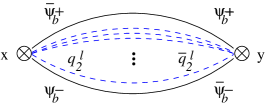
Figure 2.6: One of the four graphs of the correlator $\langle{\cal C}^{l}(x)\bar{\cal C}^{l}(y)\rangle$.

We show ${\cal O}(g^{2})$ nonrenormalization for ${\cal C}^{l}$ with $l=0$ for which $q_{2}$ exchanges are absent. The relevant propagators are

$$\langle v_{M}(x)v_{N}(y)\rangle=\frac{\eta_{MN}}{(2\pi)^{2}(x-y)^{2}}\,,\qquad\langle q_{1}(x)\bar{q}_{1}(y)\rangle=\frac{1}{(2\pi)^{2}(x-y)^{2}}\,,$$ (2.124)

$$\langle\psi_{\alpha}(x)\bar{\psi}_{\beta}(y)\rangle=\frac{i}{2\pi}\frac{\rho^{M}_{\alpha\beta}(x-y)_{M}}{(x-y)^{2}}\,,$$ (2.125)

with $\eta_{MN}={\rm diag(+1,-1)}$, Pauli matrices $\rho^{M}(M=0,1)$ defined in App. A.5, and defect coordinates $x,y$. The four-dimensional propagators in Eq. (2.124) are pinned to the defect. The Feynman rules for the vertices can be read off from the defect action in component form derived in App. A.7.

First we note that, similar as in ${\cal N}=4$, $d=4$ SYM theory [154], there are no one-loop self-energy corrections to the defect fermionic propagator $\langle\bar{\psi}_{b}\psi_{b}\rangle$. Self-energy corrections involving a gaugino propagator are cancelled by those involving a $\psi^{q_{1}}$ propagator which is the fermion of the superfield $Q_{1}$. There are also self-energy graphs with $q_{1}$ and $\sigma$ propagators which arise from the ambient scalars coupling to the defect. These cancel each other, too.

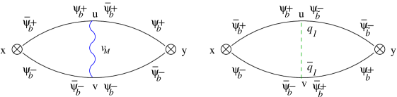
Figure 2.7: First order corrections to the correlator $\langle{\cal C}^{l}(x)\bar{\cal C}^{l}(y)\rangle$ for $l=0$.

However, we have two possible corrections from exchange graphs as shown in Fig. 2.7. Note that in Fig. 2.7, two different contributions to ${\cal C}^{l}$ ($l=0$) are depicted at the point $y$, which originate from different terms in the sum (2.123). These graphs include an ambient gauge boson exchange and an ambient scalar exchange. There is no $\sigma$ exchange contributing to the correlator $\langle{\cal C}^{l}(x){\cal C}^{l}(y)\rangle$ (for $l=0$). In fact, it may be shown that for each of the components of ${\cal C}^{\mu l}$, there is either a $\sigma$ or a $q_{1}$ exchange. For all of the components, the vector exchange is cancelled by one of these scalar exchanges while the other one vanishes.

For the gauge boson exchange in Fig. 2.7a we find the contribution

$$\frac{1}{2}\int d^{2}ud^{2}v\, \frac{\rho_{++}\cdot(x-u)}{2\pi(x-u)^{2}}(-\frac{1}{2}g\rho^{M}_{++})\frac{\eta_{MN}}{(2\pi)^{2}(u-v)^{2}}(-\frac{1}{2}g\rho^{N}_{--})\frac{\rho_{++}\cdot(u-y)}{2\pi(u-y)^{2}}$$

$$\times\frac{\rho_{--}\cdot(x-v)}{2\pi(x-v)^{2}}\frac{\rho_{--}\cdot(v-y)}{2\pi(v-y)^{2}}\,.$$ (2.126)

The overall factor $\frac{1}{2}$ comes from the definition $v_{M}=\frac{1}{\sqrt{2}}v^{\prime}_{M}$.

Let us now consider the contribution from the $q_{1}$ exchange in Fig. 2.7b which is given by

$$-\int d^{2}ud^{2}v\, \frac{\rho_{++}\cdot(x-u)}{2\pi(x-u)^{2}}(\frac{1}{2}ig)\frac{1}{(2\pi)^{2}(u-v)^{2}}(-\frac{1}{2}ig)\frac{\rho_{--}\cdot(u-y)}{2\pi(u-y)^{2}}$$

$$\times\frac{\rho_{--}\cdot(x-v)}{2\pi(x-v)^{2}}\frac{\rho_{++}\cdot(v-y)}{2\pi(v-y)^{2}}\,.$$ (2.127)

Note that the operator at the external point $y$ in the graph of Fig. 2.7b is the conjugate of the first term in Eq. (2.123) which leads to the minus sign in front of the integral in Eq. (2.127). In Fig. 2.7a both external vertices have a minus sign, whereas in Fig. 2.7b the vertices have opposite signs. Since $\eta_{MN}\rho^{M}_{++}\rho^{N}_{--}=2$, the vector exchange exactly cancels the contribution from the scalar exchange.

Nonrenormalization of correlators of ${\cal C}^{\mu l}$ with $l\geq 1$ is more difficult to show. As was shown for the operators ${\rm Tr\,}X^{k}$ in ${\cal N}=4$ super Yang-Mills theory [154, 155], there are no exchanges between the ambient propagators $\langle q_{2}(x)\bar{q}_{2}(y)\rangle$ within the correlator $\langle{\cal C}^{l}(x)\bar{\cal C}^{l}(y)\rangle$. However, one could think of a gauge boson exchange between a fermionic defect and a bosonic ambient propagator. If we do not work in Wess-Zumino gauge then there is an additional interaction of the defect fermions with a scalar $C$ which is the lowest component of the gauge superfield $V$. Keeping this in mind we expect that a CD exchange [154] cancels the above gauge boson exchange.

2.5.6 Vanishing of odd correlators of the BPS primaries ${\cal C}^{\mu l}$

Another property of the BPS primaries ${\cal C}^{\mu l}$ is the vanishing of all $(2k+1)$-point functions ($k\in\mathbb{N}$). Only even $n$-point functions may differ from zero. On the gravity side this can be seen by studying once more the DBI action of the probe D3-brane. Due to the expansion of the cosines of the angular fluctuations $\theta,\phi,\rho$, and $\chi$ in the determinant, the BI action contains only even powers of the fluctuations, see Eq. (2.16). This implies vanishing odd couplings for the Kaluza-Klein modes which, via the AdS/CFT correspondence, implies vanishing odd $n$-point functions on the field-theory side. In the dual conformal field theory these Kaluza-Klein modes correspond to the BPS primary operators ${\cal C}^{\mu l}$. Again we restrict to the component ${\cal C}^{l}\equiv{\cal C}^{1l}$.

On the field theory side too, one finds for instance that the three-point function $\langle{\cal C}^{l_{1}}(x){\cal C}^{l_{2}}(y){\cal C}^{l_{3}}(z)\rangle$ is absent. This is due to a global $U(1)$ symmetry of the action,

$$B \rightarrow e^{i\frac{\phi}{2}}B\,,\qquad\tilde{B}\rightarrow e^{i\frac{\phi}{2}}\tilde{B}\,,\qquad Q_{1}\rightarrow e^{-i\phi}Q_{1}\,,\qquad Q_{2}\rightarrow e^{i\phi}Q_{2}\,,$$ (2.128)

with all other fields being singlets under this symmetry. If we choose $\phi=\pi$ then ${\cal C}^{l}\rightarrow(e^{i\pi})^{l+1}{\cal C}^{l}$ and the three-point function transforms as

$$\langle{\cal C}^{l_{1}}(x){\cal C}^{l_{2}}(y){\cal C}^{l_{3}}(z)\rangle\rightarrow(-1)^{l_{1}+l_{2}+l_{3}+1}\langle{\cal C}^{l_{1}}(x){\cal C}^{l_{2}}(y){\cal C}^{l_{3}}(z)\rangle\,.$$ (2.129)

Since $l_{1}+l_{2}+l_{3}$ must be even, $(-1)^{l_{1}+l_{2}+l_{3}+1}=-1$ and $\langle{\cal C}^{l_{1}}(x){\cal C}^{l_{2}}(y){\cal C}^{l_{3}}(z)\rangle$ vanishes. Though we have restricted the discussion on ${\cal C}^{1l}$, the statement also holds for the other components. This is guaranteed by the fact that ${\cal C}^{\mu l}$ transforms as a vector under the $SO(4)$ R-symmetry group.

2.5.7 Summary and discussion of the AdS/CFT dictionary

Table 2.3 summarizes the fluctuations of the KK modes and their dual operators. The angular fluctuations of the probe $S^{1}$ embedding inside $S^{5}$ are dual to $1/4$ BPS primaries ${\cal C}^{\mu l}$. The $\Delta=3-l$ fluctuations of the embedding of $AdS_{3}$ inside $AdS_{5}$ are dual to ${\cal G}^{l}$ which are two-supercharge descendants of these primaries. The $\Delta=l-1$ fluctuations of the embedding of $AdS_{3}$ inside $AdS_{5}$ are not dual to conformal operators which correspond to states in the Hilbert space. Naively the dual operators ${\cal B}^{l}$ look like $1/2$ BPS (chiral) primaries, but in fact they contain massless defect scalars which do not give rise to power law correlation functions. These massless scalars and their dual fluctuations include an entry ${\cal B}^{1}$ which parameterizes the classical Higgs branch. The fluctuations ${\cal B}^{l}$ for $l>1$ correspond to other holomorphic curves $w=c_{l}/y^{l}$, however we do not (as yet) have a clear interpretation for these in the defect CFT. Lastly, the operator ${\cal J}^{M}_{B}$ which is dual to the gauge field fluctuations on $AdS_{3}$ is a descendant of the dimensionless operator $\bar{b}b+\tilde{b}\bar{\tilde{b}}$, which has a logarithmic two-point function and is not a primary operator although formally it trivially satisfies the BPS bounds.

fluctuations	$\Delta$	$l$	$(j_{1},j_{2})_{\cal J}$	operator	interpretation
$S^{1}\subset S^{5}$	$l+1$	$l\geq 0$	$(\frac{1}{2},\frac{1}{2})_{l}$	${\cal C}^{\mu l}$	$1/4$ BPS primary
$AdS_{3}\subset AdS_{5}$	$3-l$	$l\leq 1$	$(0,0)_{l+1}$	${\cal G}^{l}$	descendant
	$l-1$	$l\geq 1$	$(0,0)_{l+1}$	${\cal B}^{l}$	classical Higgs branch
gauge field	$l+1$	$l\geq 0$	$(0,0)_{l}$	${\cal J}_{B}^{Ml}$	—

Table 2.3: Summary of fluctuation modes and field theory operators with coincident quantum numbers.

3 Fundamental matter in the AdS/CFT correspondence

One of the main objectives of this paper is the inclusion of particles in the fundamental representation of the gauge group into the AdS/CFT correspondence. This is an indispensable necessity to study QCD in terms of its holographic dual. As we have seen in the last chapter, fundamental representations can be introduced by embedding a probe brane on an $AdS_{d}$ subspace of the full $AdS_{D}$ geometry, where $d\leq D$ and the boundary of $AdS_{d}$ is part of the boundary of the $AdS_{D}$. Embeddings for which $d=D$ give rise to a dual field theory with “quarks” that are free to move in all spacetime dimensions. The D3-D7 brane intersection realises such an embedding in its near-horizon geometry, where it wraps an $AdS_{5}\times S^{3}$ submanifold. In order to study non-perturbative effects in large $N$ QCD-like theories, we now embed a D7 probe in two non-supersymmetric supergravity backgrounds, both exhibiting confinement of fundamental matter. This allows us to numerically compute quark condensates and meson spectra.

The organisation of this chapter is as follows. In Sec. 3.1 we discuss explicitly the holography of the D3-D7 intersection. Here we specialize the general discussion of the D3-D$p$ brane system of the previous chapter to $p=7$, i.e. we study D7-probes in the AdS/CFT Correspondence. We demonstrate our numerical techniques by a supergravity computation of the meson spectrum in the standard AdS/CFT correspondence. In Sec. 3.2 we consider D7-branes in the AdS Schwarzschild black hole background. We find a first order phase transition in the dual field theory. We compute the quark condensate and the meson spectrum. In Sec. 3.3 we study D7-brane probes in the Constable-Myers background [20]. We demonstrate spontaneous $U(1)_{A}$ chiral symmetry breaking and identify the corresponding Goldstone boson in the meson spectrum. We summarize our results in Ch. 5.

3.1 AdS/CFT duality for an ${\mathcal{N}}=2$ gauge theory with fundamental matter

3.1.1 The D3-D7 brane configuration

It was first observed in [51] that one can obtain a holographic dual of a four-dimensional Yang-Mills theory with fundamental matter by taking the near-horizon limit of a system of intersecting D3 and D7-branes. We first review some of the features of this duality, and then test numerical techniques which we will use later to study deformations of this duality.

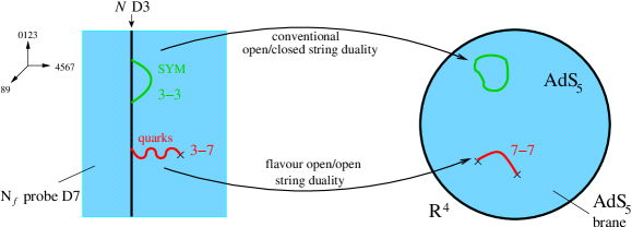
Figure 3.1: Holography of the D3–D7 brane configuration.

According to the general description of a D3-D$p$ brane intersection, see Sec. 2.1, we consider a stack of $N$ D3-branes spanning the directions $x^{0},x^{1},x^{2},x^{3}$ and another stack of $N_{f}$ D7-branes spanning the directions $x^{0},...,x^{7}$. This is shown in the left picture of Fig. 3.1. The low-energy dynamics of open strings in this setting is described by a ${\mathcal{N}}=2$ super Yang-Mills theory. This theory contains the degrees of freedom of the ${\mathcal{N}}=4$ theory, namely an ${\mathcal{N}}=2$ vector multiplet and an ${\mathcal{N}}=2$ adjoint hypermultiplet, as well as $N_{f}$ ${\mathcal{N}}=2$ hypermultiplets in the fundamental representation of $SU(N)$. The theory is conformal in the limit $N\rightarrow\infty$ with $N_{f}$ fixed. There is an $SU(2)\times U(1)$ R-symmetry. The $U(1)$ R-symmetry acts as a chiral rotation on the “quarks”, which are the fermionic components of the ${\mathcal{N}}=2$ hypermultiplet composed of fundamental and anti-fundamental chiral superfields $Q$ and $\tilde{Q}$. This symmetry also acts as a phase rotation on the scalar component of one of the adjoint chiral superfields. When the D7-branes are separated from the D3-branes in the two mutually transverse directions $X^{8}$ and $X^{9}$, the fields $Q,\tilde{Q}$ become massive, explicitly breaking the $U(1)$ R-symmetry and conformal invariance. As shown in [51], the ${\mathcal{N}}=2$ theory as well as its renormalization group flow have an elegant holographic description.

This holographic description is obtained as follows. In the limit of large $N$ at fixed but large ’t Hooft coupling $\lambda=g^{2}N\gg 1$, the D3-branes may be replaced with their near-horizon $AdS_{5}\times S^{5}$ geometry given by

$$ds^{2}=\frac{r^{2}}{L^{2}}(-dt^{2}+dx_{1}^{2}+dx_{2}^{2}+dx_{3}^{2})+\frac{L^{2}}{r^{2}}d\vec{y}^{2}\,,$$ (3.1)

where $\vec{y}=(X^{4},\cdots,X^{9})$, $r^{2}\equiv\vec{y}^{2}$, and $L$ the radius of curvature. It will be convenient to write the transverse metric $d\vec{y}^{2}$ in the following way

$$d\vec{y}^{2}=d\rho^{2}+\rho^{2}d\Omega_{3}^{2}+dy_{5}^{2}+dy_{6}^{2}\,,$$ (3.2)

where $d\Omega_{3}^{2}$ is a three-sphere metric and $r^{2}=\rho^{2}+y_{5}^{2}+y_{6}^{2}$. Since the number $N_{f}$ of D7-branes is finite, their back-reaction on the geometry can be effectively ignored.

For massless flavours, the D7-brane embedding in the D3-metric (2.4) is given by $y^{5}=y^{6}=0$ (corresponding to $X^{8}=X^{9}=0$). In the $AdS_{5}\times S^{5}$ geometry, the induced geometry on the D7-brane is given by the metric (2.8) (for $k=3$) which is $AdS_{5}\times S^{3}$. The D7-brane fills $AdS_{5}$, while wrapping a great three-sphere of the $S^{5}$. The isometries of the $AdS_{5}\times S^{5}$ metric which preserve the embedding correspond to the conformal group and R-symmetries of the ${\mathcal{N}}=2$ gauge theory. The conformal group $SO(2,4)$ is the isometry group of $AdS_{5}$, while the $SU(2)\times U(1)$ R-symmetry corresponds to the rotations of the $S^{3}$ inside $S^{5}$ and rotations of the $y^{5},y^{6}$ coordinates.

The holographic description for massive flavours is found by considering the D7-brane embedding $y^{5}=X^{8}=0$, $y^{6}=X^{9}=m$. In this case the D7-geometry is still $AdS_{5}\times S^{3}$ in the $r\rightarrow\infty$ region corresponding to the ultraviolet. However, from the induced metric on the D7-brane,

$$ds^{2}_{probe}=\frac{\rho^{2}+m^{2}}{L^{2}}(-dt^{2}+dx_{1}^{2}+dx_{2}^{2}+dx_{3}^{2})+\frac{L^{2}}{\rho^{2}+m^{2}}(d\rho^{2}+\rho^{2}d\Omega_{3}^{2})\,,$$ (3.3)

we see that the radius of the three-sphere vanishes at $\rho=0$ or, equivalently, at $r=m$. This is possible because the $S^{3}$ is contractible within the $S^{5}$ of the full ten dimensional geometry. The D7-brane “ends” at the value of $r$ at which the $S^{3}$ collapses, meaning that it does not fill all of $AdS_{5}$, but only a region outside a core of radius $r=m$. This is consistent with the fact that the fundamental degrees of freedom decouple at energies below $m$. Note that although the D7-brane ends at $r=m$, the D7-geometry is perfectly smooth, as is illustrated in Fig. 3.2. In the massive case, the conformal and $U(1)$ symmetries are broken, and the D7 embedding is no longer invariant under the corresponding isometries.

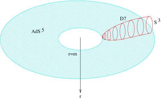
Figure 3.2: The D7 embedding in $AdS_{5}\times S^{5}$ for $m\neq 0$. The figure shows the modification of the $AdS_{5}$ brane embedding on the r.h.s. of Fig. 3.1 in the case of massive quarks.

3.1.2 Testing numerical methods: Mesons in the D3-D7 intersection

In this chapter we will numerically compute condensates and meson spectra in deformations of the duality discussed above. Therefore we first test these numerical techniques against some exact results in the undeformed case.

To study the implications of the classical D7 probe dynamics for the dual field theory, we now evaluate the scalar contributions to the Dirac-Born-Infeld (DBI) action for the D7-brane in the $AdS_{5}\times S^{5}$ background. We work in static gauge where the world-volume coordinates of the brane are identified with the spacetime coordinates by $\xi^{a}\sim t,x_{1},x_{2},x_{3},y_{1},...,y_{4}$. The DBI action (2.13) for $p=7$ is then

$$S_{D7} = -T_{D7}\int d^{8}\xi\sqrt{-{\rm det}(g^{PB}_{ab})}=-T_{D7}\int d^{8}\xi\sqrt{-\det g_{ab}}\sqrt{1+g^{ab}\partial_{a}Z^{i}\partial_{b}Z^{j}g_{ij}}$$ (3.4)

$$= -T_{D7}\int d^{8}\xi\leavevmode\nobreak\ \epsilon_{3}\leavevmode\nobreak\ \rho^{3}\sqrt{1+{\frac{g^{ab}}{\rho^{2}+y_{5}^{2}+y_{6}^{2}}}(\partial_{a}y_{5}\partial_{b}y_{5}+\partial_{a}y_{6}\partial_{b}y_{6})}\,,$$

where $Z^{i}$ are the transverse coordinates $y_{5},y_{6}$. The metrics $g_{ab}$ and $g_{ij}$ are the $AdS_{5}\times S^{5}$ metric restricted to eight and two dimensions, respectively (set either $dZ^{i}=0$ or $d\xi^{a}=0$). The factor $\epsilon_{3}$ is the determinant from the three sphere. The ground state configuration of the D7-brane is given by the solution of the Euler-Lagrange equation with dependence only on the $\rho$ variable. In this case the equations of motion become (use $g^{\rho\rho}=r^{2}=\rho^{2}+y_{5}^{2}+y_{6}^{2}$)

$${\frac{d}{d\rho}}\left[{\rho^{3}\over\sqrt{1+\left({dy_{6}\over d\rho}\right)^{2}}}{dy_{6}\over d\rho}\right]=0\,,$$ (3.5)

where we consider solutions with $y_{5}=0$ only. Recall that the $U(1)$ R-symmetry corresponds to rotations in the $y^{5}$–$y^{6}$-plane.

The equations of motion have asymptotic ($\rho\rightarrow\infty$) solutions of the form

$$y_{6}=m+{\frac{c}{\rho^{2}}}\,.$$ (3.6)

The identification of these constants as field theory operators requires a coordinate transformation because the scalar kinetic term is not of the usual canonical AdS form. Transforming to the coordinates of [51] in which the kinetic term has canonical form, we see that $m$ has dimension 1 and $c$ has dimension 3. The scalars are then identified [94] with the quark mass $m_{q}$ and condensate $\langle\bar{\psi}\psi\rangle$, respectively, in agreement with the usual AdS/CFT dictionary. The dimension three operator ${\cal C}^{0}=\bar{\psi}\psi$ is the higher-dimensional analog of the operator ${\cal C}^{\mu 0}$ as given by Eq. (2.92) and is dual to $S^{3}$ fluctuations inside $S^{5}$.

Figure 3.3: Numerical solutions of the equations of motion in AdS showing that in the presence of a condensate asymptotically the solutions are divergent. The regular solution is the mass only solution.

$y_{6}$                                                                                    $\rho$

Note that $y_{6}(\rho)=m$ is an exact solution of the equations of motion, corresponding to the embedding [51] reviewed above. On the other hand there should be something ill-behaved about the solutions with non-zero $c$, since a quark condensate is forbidden by supersymmetry. In Fig. 3.3 we plot numerical solutions of the equations of motion (obtained by a shooting technique using Mathematica) for solutions with non-zero $c$, and find that they are divergent. The divergence of these solutions is not, by itself, pathological because the variable $y_{6}$ is just the location of the D7-brane. However the AdS radius $r^{2}=y_{6}(\rho)^{2}+\rho^{2}$ is not monotonically increasing as a function of $\rho$ for the divergent solutions. This means that these solutions have no interpretation as a renormalization group flow, or as a vacuum of the dual field theory. As expected, the mass only solution is the only well-behaved solution.

The other exact result which we wish to test numerically is the meson spectrum. In order to find the states with zero spin on the $S^{3}$, one looks for normalizable solutions of the equations of motion of the form

$$y_{6}+iy_{5}=m+f(\rho)e^{ikx},\hskip 28.45274ptM^{2}=-k^{2}\,,$$ (3.7)

where one linearizes in the small fluctuation $f(\rho)$. The linearized equation of motion is

$$\partial_{\rho}^{2}f(\rho)+{\frac{3}{\rho}}\partial_{\rho}f(\rho)+{\frac{M^{2}}{(\rho^{2}+m^{2})^{2}}}f(\rho)=0\,.$$ (3.8)

This was solved exactly in [86], where it was shown that the solutions can be written as hypergeometric functions

$$f(\rho)={\frac{A}{(\rho^{2}+1)^{n+1}}}F(-n-1,-n;2,-\rho^{2})$$ (3.9)

with $A$ a constant. The exact mass spectrum is then given by

$$M=2m\sqrt{(n+1)(n+2)},\hskip 28.45274ptn=0,1,2,\dots\,.$$ (3.10)

We are interested in whether we can reproduce this result numerically, via a shooting technique. The equation of motion can be solved numerically subject to boundary conditions $f(\rho)\sim c/\rho^{2}$ at large $\rho$ indicating that the meson is a quark bilinear of dimension 3 in the UV. Solutions of the equation must be regular at all $\rho$ so the allowed $M^{2}$ solutions can be found by tuning to these regular forms. The result (3.10) is easily reproduced to 2 significant figures. We show an example of the method in action in Fig. 3.4.

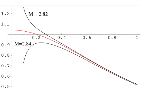
Figure 3.4: Numerical solutions of the meson equation of motion for different values of $M$ showing the identification of the first bound state mass. The exact regular solution is plotted between the two numerical flows.

$f(\rho)$                                                                               $\rho$

3.2 The AdS-Schwarzschild Solution

3.2.1 The background

We now move on to study quark condensates and mesons in a non-supersymmetric deformation of the AdS/CFT correspondence and study the AdS-Schwarzschild black hole solution. This geometry is dual to the ${\cal N}=4$ gauge theory at finite temperature [16], which is in the same universality class as pure three-dimensional QCD.

The Euclidean AdS-Schwarzschild solution is given by

$$ds^{2}=K(r)d\tau^{2}+{\frac{dr^{2}}{K(r)}}+r^{2}dx_{\parallel}^{2}+d\Omega_{5}^{2}\,,$$ (3.11)

where

$$K(r)=r^{2}-{\frac{b^{4}}{r^{2}}}\,.$$ (3.12)

This space-time is smooth and complete if $\tau$ is periodic with period $\pi b$. Note that the $S^{1}$ parameterized by $\tau$ collapses at $r=b$. The fact that the geometry “ends” at $r=b$ is responsible for the existence of an area law for the Wilson loop and a mass gap in the dual field theory (see [16]). The period of $\tau$ is equivalent to the inverse temperature in the dual ${\mathcal{N}}=4$ gauge theory. The parameter $b$ sets the scale of the deformation and for convenience in the numerical work below we shall set it equal to 1. At finite temperature, the fermions have anti-periodic boundary conditions in the Euclidean time direction and become massive upon dimensional reduction to three dimensions. The adjoint scalars also become massive at one loop. Thus in the high-temperature limit, the adjoint fermions and scalars decouple, leaving pure three-dimensional QCD.

We now introduce a D7-brane into this background, which corresponds to the addition of matter in the fundamental representation. The dual gauge theory is the ${\mathcal{N}}=2$ gauge theory of Karch and Katz at finite temperature. Note that the fermions in the fundamental representation also have anti-periodic boundary conditions in the Euclidean time direction. Thus these also decouple in the high-temperature limit, as do the fundamental scalars which get masses at one loop, leaving pure QCD₃ as before. Thus in this particular case we are not interested in the high-temperature limit, but only the region accessible to supergravity and Dirac-Born-Infeld theory. Although the dual field theory cannot be viewed as a three-dimensional gauge theory with light quarks, it is nevertheless a four-dimensional non-supersymmetric gauge theory with confined degrees of freedom in the fundamental representation. This provides an interesting, if exotic, setting to compute quark condensates and meson spectra using Dirac-Born-Infeld theory. The Constable-Myers background which we will consider later turns out to have more realistic properties.

3.2.2 Embedding of a D7-brane

To embed a D7-brane in the AdS black-hole background it is useful to recast the metric (3.11) to a form with an explicit flat 6-plane. To this end, we change variables from $r$ to $w$, such that

$${\frac{dw}{w}}\equiv{\frac{rdr}{(r^{4}-b^{4})^{1/2}}}\,,$$ (3.13)

which is solved by

$$2w^{2}=r^{2}+\sqrt{r^{4}-b^{4}}\,.$$ (3.14)

The metric is then

$$ds^{2}=\left(w^{2}+\frac{b^{4}}{4w^{2}}\right)d\vec{x}^{2}+\frac{(4w^{4}-b^{4})^{2}}{4w^{2}(4w^{4}+b^{4})}dt^{2}+\frac{1}{w^{2}}(\sum_{i=1}^{6}dw_{i}^{2})\,,$$ (3.15)

where $\sum_{i}dw_{i}^{2}=dw^{2}+w^{2}d\Omega_{5}^{2}$, which for reasons of convenience will also be written as $d\rho^{2}+\rho^{2}d\Omega_{3}^{2}+dw_{5}^{2}+dw_{6}^{2}$ where $d\Omega_{3}^{2}$ is the unit three-sphere metric. The AdS black hole geometry asymptotically approaches $AdS_{5}\times S^{5}$ at large $w$. Here the background becomes supersymmetric, and the D7 embedding should approach that discussed in [51]. The asymptotic solution has the form $w_{6}=m,w_{5}=0$, where $m$ should be interpreted as a bare quark mass. To take into account the deformation, we will consider a more general ansatz for the embedding of the form $w_{6}=w_{6}(\rho),w_{5}=0$, with the function $w_{6}(\rho)$ to be determined numerically. The DBI action for the orthogonal directions $w_{5},w_{6}$ is

$$S_{D7} =-\mu_{7}\int d^{8}\xi\leavevmode\nobreak\ \epsilon_{3}\leavevmode\nobreak\ {\cal G}(\rho,w_{5},w_{6})$$ (3.16)

$$\times\left(1+{g^{ab}\over(\rho^{2}+w_{5}^{2}+w_{6}^{2})}\partial_{a}w_{5}\partial_{b}w_{5}+{g^{ab}\over(\rho^{2}+w_{5}^{2}+w_{6}^{2})}\partial_{a}w_{6}\partial_{b}w_{6}\right)^{1/2}\,,$$

where the determinant of the metric is given by

$${\cal G}(\rho,w_{5},w_{6}) =\sqrt{g_{tt}g_{xx}^{3}\rho^{6}\over(\rho^{2}+w_{5}^{2}+w_{6}^{2})^{4}}$$

$$=\rho^{3}{(4(\rho^{2}+w_{5}^{2}+w_{6}^{2})^{2}+b^{4})(4(\rho^{2}+w_{5}^{2}+w_{6}^{2})^{2}-b^{4})\over 16(\rho^{2}+w_{5}^{2}+w_{6}^{2})^{4}}\,.$$ (3.17)

With the ansatz $w_{5}=0$ and $w_{6}=w_{6}(\rho)$, the equation of motion becomes

$${d\over d\rho}\left[{\cal G}(\rho,w_{6})\sqrt{1\over 1+\left({dw_{6}\over d\rho}\right)^{2}}{dw_{6}\over d\rho}\right]-\sqrt{1+\left({dw_{6}\over d\rho}\right)^{2}}{b^{8}\rho^{3}w_{6}\over 2(\rho^{2}+w_{6}^{2})^{5}}=0\,.$$ (3.18)

The solutions of this equation determine the induced metric on the D7 brane which is given by

$$ds^{2}=\left(\tilde{w}^{2}+\frac{b^{4}}{4\tilde{w}^{2}}\right)d\vec{x}^{2}+\frac{(4\tilde{w}^{4}-b^{4})^{2}}{4\tilde{w}^{2}(4\tilde{w}^{4}+b^{4})}dt^{2}+\frac{1+(\partial_{\rho}w_{6})^{2}}{\tilde{w}^{2}}d\rho^{2}+\frac{\rho^{2}}{\tilde{w}^{2}}d\Omega_{3}^{2}\,,$$ (3.19)

with $\tilde{w}^{2}=\rho^{2}+w_{6}^{2}(\rho)$. The D7-brane metric becomes $AdS_{5}\times S^{3}$ for $\rho\gg b,m$.

3.2.3 Karch-Katz solutions versus condensate solutions

Before computing the explicit D7-brane solutions, we remark that there are several possibilities for the topology of the D7-brane embedding which we illustrate in Fig. 3.5.

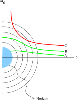
Figure 3.5: Different possibilities for solutions of the D7-brane equations of motion. The semicircles are lines of constant $r$, which should be interpreted as a scale in the dual Yang-Mills theory. The curves of type $A,B$ have an interpretations as an RG flow, while the curve $C$ does not.

The UV asymptotic (large $\rho$) solution, where the geometry returns to $AdS_{5}\times S^{5}$, is of the form

$$w_{6}(\rho)\sim m+\frac{c}{\rho^{2}}\,.$$ (3.20)

The parameters $m$ and $c$ have the interpretation as a quark mass and bilinear quark condensate respectively, as discussed below equation (3.6). These parameters can be taken as the boundary conditions for the second order differential equation (3.18), which we solve using a numerical shooting technique. Of course the physical solutions should not have arbitrary $m$ and $c$. The condition which we use to identify physical solutions is that the D7-brane embedding should have an interpretation as a RG flow. This implies for instance that if one slices the D7-brane geometry at a fixed value of $w^{2}$, or equivalently at a fixed value of $w_{6}^{2}+\rho^{2}$, one should obtain at most one copy of the geometry $R^{4}\times S^{3}$. In other words, $w^{2}=\rho^{2}+w_{6}(\rho)^{2}$ should be a monotonically increasing function of $\rho$. This is certainly not the case for divergent solutions. Such solutions are not in correspondence with a vacuum of the dual gauge theory and are discarded.

There are then two possible forms of regular solutions. The geometry in which the D7-brane is embedded has the boundary topology $R^{3}\times S^{1}\times S^{5}$, which contains the D7-brane boundary $R^{3}\times S^{1}\times S^{3}$. Recall that the $S^{3}$ is contractible within $S^{5}$. Furthermore the $S^{1}$ is contractible within the bulk geometry and shrinks to zero as one approaches the horizon $r=b$ (i.e. $w=b/\sqrt{2}$). The D7-brane may either “end” at some $r>b$ if the $S^{3}$ collapses, or it may continue all the way to the horizon where the $S^{1}$ collapses but the $S^{3}$ has finite size. In other words, the D7-topology may be either $R^{3}\times B^{4}\times S^{1}$ or $R^{3}\times S^{3}\times B^{2}$. The former is the type found in [51]. As one might expect, this topology occurs when the quark mass $m$ is sufficiently large compared to $b$. In this case, the $S^{3}$ of the D7-brane contracts to zero size in the asymptotic region where the deformation of $AdS_{5}\times S^{5}$ is negligible. We shall find the other topology for sufficiently small $m$.

Figure 3.6: An example (for $m=0.6$) of the different flow behaviour around the regular (physical) solution.

$w_{6}$                                                                                 $\rho$

For any chosen value of $m$, we find only a discrete choice of $c$ which gives a regular solution that can be interpreted as an RG flow. In Fig. 3.6 we show sample numerical flows used to identify a regular solution.

For the regular solutions the D7-brane either ends at the horizon,

$$w_{6}^{2}+\rho^{2}=\frac{1}{2}b^{2}\,,$$ (3.21)

at which the $S^{1}$ collapses, or ends at a point outside the horizon,

$$\rho=0\,,\qquad w_{6}^{2}\geq\frac{1}{2}b^{2},$$ (3.22)

at which the $S^{3}$ collapses (see (3.19)). Both types of solution are illustrated in Fig. 3.7 for several choices of $m$. We choose units such that $b=1$. We refer to solutions with collapsing $S^{3}$ as Karch-Katz solutions, and solutions with collapsing $S^{1}$ as “condensate” solutions, for reasons that will become apparent shortly. Note that the boundary between the Karch-Katz and condensate solutions is at a critical value of the mass $m=m_{\rm crit}$ such that $w_{6}(\rho=0)=\sqrt{1/2}b$. In this case both the $S^{1}$ and $S^{3}$ collapse simultaneously. Numerically, we find $m_{\rm crit}\approx 0.92$. While the Karch-Katz solutions are (approximately) constant for all values of $\rho$, the condensate solutions bend towards the horizon for small $\rho$. As expected, the black hole exerts an attractive force on the D7-brane.

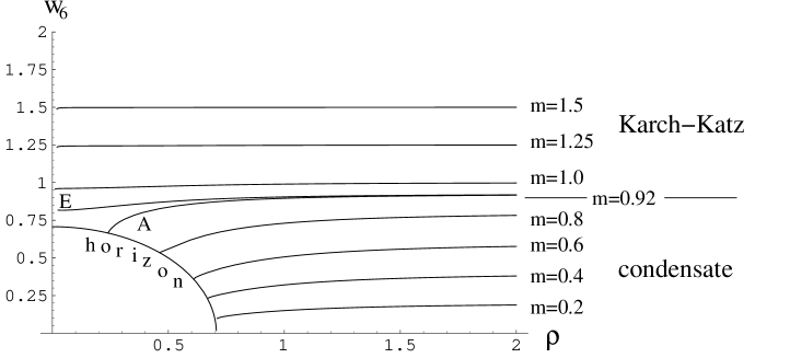
Figure 3.7: Two classes of regular solutions in the AdS black hole background. The quark mass $m_{q}$ is the parameter $m$ in units of $\Lambda\equiv\frac{b/\sqrt{2}}{2\pi\alpha^{\prime}}$: $m_{q}=m\Lambda$. Numerically we set $\Lambda=1/\sqrt{2}$.

As mentioned above, the dual gauge theory is considered at finite temperature. The same gauge theory at zero temperature is dual to supergravity on the near-horizon geometry of solitonic D3-branes instead of thermal D3-branes (from which the AdS black hole descends in the case $T>0$). Solitonic D3-branes exert a repulsive force on the D7-branes and one would obtain a plot similar to Fig. 3.11. This has been studied in detail in [101] for thermal and solitonic D4-branes.

There is an exact solution of the equation of motion $w_{6}=0$ which is regular and corresponds to $m=c=0$. Thus there is no condensate when the quarks are massless (from the four-dimensional point of view). This should not be disappointing, since the theory is not in the same universality class as QCD₃ with light quarks. The quarks obtain a mass of order the temperature which will tend to suppress the formation of a condensate. For non-zero $m$ we obtain the solutions numerically.

Phase transitions in QCD-like theories at finite temperature

The dependence of the condensate on the mass is illustrated in Fig. 3.8a. We find that as $m$ increases, the condensate $c$ initially increases and then decreases again. At sufficiently large $m$, the condensate becomes negligible, which is to be expected as the D7-brane ends in the region where the deformation of AdS is small. Recall that there is no condensate in the Yang-Mills theory with unbroken ${\mathcal{N}}=2$ supersymmetry described by D7-branes in un-deformed AdS.

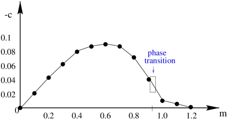
Figure 3.8: A plot of the parameter $c$ vs $m$ for the regular solutions in AdS Schwarzschild. The linear fit between points is just to guide the eye. The right plot zooms in around $m_{\rm crit}\approx 0.92$.

Since the D7-brane topology changes as one crosses $m_{\rm crit}$, one might expect a phase transition to occur at this point. Zooming in around $m_{\rm crit}$, we see in Fig. 3.8b that $c$ is multi-valued around the critical mass $m_{\rm crit}$. This means that two graphs in Fig. 3.7 can have the same asymptotic behaviour but a different behaviour at small values of $\rho$. For instance, the value of $c$ at the point $A$ in Fig. 3.8b corresponds to the graph $A$ in Fig. 3.7 which ends at the horizon, while $c$ at the point $E$ is associated with the graph $E$ which ends above the horizon. The dashed line between $A$ and $E$ is obtained by the Maxwell construction and corresponds to the equilibrium transition between the two phases. In this regime both phases are present. We can reformulate this result by keeping the quark mass $m_{q}$ fixed and vary the horizon $b/\sqrt{2}$, i.e. the temperature $T\sim(\pi b)^{-1}$. Then the $c$-$m$ plot can also be considered as a plot of the condensate $c$ in dependence of the temperature $T$. During the phase transition between the points $A$ and $E$ the condensate decreases while the temperature remains constant. The graph in Fig. 3.8b looks quite similar to an isotherm of a fluid in a pressure-volume diagram. As in the case of a fluid the phase transition is discontinuous and thus of first order. A similar behaviour has been found in the thermal D4-brane background studied in [101]. Such phase transitions seem to be a universal feature of QCD-like theories at finite temperature.

3.2.4 Meson spectrum in the AdS black-hole background

The meson spectrum can be found by solving the linearized equations of motion for small fluctuations about the D7-embeddings found above. Let us consider the fluctuations of the variable $w_{5}$ about the embedding, which has $w_{5}=0$. We take

$$w_{5}=f(\rho)\sin(\vec{k}\cdot\vec{x})\,.$$ (3.23)

In App. B.1 we compute the linearized (in $w_{5}$) equation of motion. We find

$$\begin{array}[]{c}{d\over d\rho}\left[{\cal G}(\rho,w_{6})\sqrt{1\over 1+\left({dw_{6}\over d\rho}\right)^{2}}{df(\rho)\over d\rho}\right]+{\cal G}(\rho,w_{6})\sqrt{1\over 1+\left({dw_{6}\over d\rho}\right)^{2}}\left({4\over 4(\rho^{2}+w_{6}^{2})^{2}+b^{4}}\right)M^{2}f(\rho)\\ \\ -\sqrt{1+\left({dw_{6}\over d\rho}\right)^{2}}{b^{8}\rho^{3}f(\rho)\over 2(\rho^{2}+w_{6}^{2})^{5}}=0\,.\end{array}$$ (3.24)

where $M^{2}=\vec{k}^{2}$. The allowed values of $\vec{k}^{2}$ are determined by requiring the solution to be normalizable and regular. Note that if the $U(1)$ symmetry which rotates $w_{5}$ and $w_{6}$ were spontaneously broken by an embedding of the asymptotic form $w_{6}\sim c/\rho^{2}$ with non-zero $c$, there would be a massless state in the spectrum associated with $w_{5}$ fluctuations. This is not the case in the present setting, since the condensate is only non-zero for non-zero quark mass $m$. Instead we find a mass gap in the meson spectrum. We have computed the meson spectrum by solving (3.24) by a numerical shooting technique. As in the Karch-Katz geometry, we seek regular solutions for $w_{5}$ which are asymptotically of the form $c/\rho^{2}$ in the presence of the background $w_{6}$ solution. The results for the meson masses are plotted in Fig. 3.9. Of course the meson mass gap here can be largely attributed to the Kaluza-Klein masses of the constituent quarks, which are of the same order as the temperature ($T\sim\pi^{-1}$ in units with $b=1$).

Figure 3.9: A plot of the $w_{5}$ meson mass vs $m$ in AdS Schwarzschild. The linear fit between points is just to guide the eye.

Thus we have seen that, while the thermal gauge background allows a quark condensate when it does not spontaneously break any symmetries, there is no chiral (parity) symmetry breaking at zero quark mass. The meson spectrum reflects this by having a mass gap - the fermions have an induced mass from the presence of finite temperature. In the subsequent discussion we will consider another background which admits light constituent quarks and has properties much closer to QCD.

3.3 The Constable-Myers Deformation

3.3.1 The background

We consider the non-supersymmetric deformed AdS geometry originally constructed in [20]. This geometry corresponds to the ${\mathcal{N}}=4$ super Yang-Mills theory deformed by the presence of a vacuum expectation value for an R-singlet operator with dimension four (such as $trF^{\mu\nu}F_{\mu\nu}$). The supergravity background has a dilaton and $S^{5}$ volume factor depending on the radial direction. In a certain parameter range, this background implies an area law for the Wilson loop and a mass-gap in the glueball spectrum. Whether the geometry, which has a naked singularity, actually describes the stable non-supersymmetric vacuum of a field theory is not well understood [20]. This is not so important from our point of view though since the geometry is a well defined gravity description of a non-supersymmetric gauge configuration. We can just ask about the behaviour of quarks in that background.

The geometry in Einstein frame is given by

$$ds^{2}= \,H^{-1/2}\left(1+{2b^{4}\over r^{4}}\right)^{\delta/4}dx_{4}^{2}$$

$$+H^{1/2}\left(1+{2b^{4}\over r^{4}}\right)^{(2-\delta)/4}{r^{2}\over\left(1+{b^{4}\over r^{4}}\right)^{1/2}}\left[{r^{6}\over(r^{4}+b^{4})^{2}}dr^{2}+d\Omega^{2}_{5}\right],$$ (3.25)

where

$$H=\left(1+{2b^{4}\over r^{4}}\right)^{\delta}-1$$ (3.26)

and with the dilaton and four-form given by

$$e^{2\phi}=e^{2\phi_{0}}\left(1+{2b^{4}\over r^{4}}\right)^{\Delta},\hskip 28.45274ptC_{(4)}=-{1\over 4}H^{-1}dt\wedge dx\wedge dy\wedge dz\,.$$ (3.27)

The parameter $b$ corresponds to the vev of the dimension 4 operator. The parameters $\Delta$ and $\delta$ are constrained by

$$\Delta^{2}+\delta^{2}=10\,.$$ (3.28)

Asymptotically the AdS curvature is given by $L^{4}=2\delta b^{4}$, so it makes sense to set (with $L=1$)

$$\delta={1\over 2b^{4}}.$$ (3.29)

As in [102] we define the fundamental energy scale $\Lambda_{b}$ as

$$\Lambda_{b}=\frac{b}{2\pi\alpha^{\prime}}\,.$$ (3.30)

$\Lambda_{b}$ is the only free parameter in the geometry and its value sets the scale of the conformal symmetry and supersymmetry breaking $\Lambda_{\rm susy}$ below which we have confinement and a discrete glueball spectrum. Since this is also approximately the scale of chiral symmetry breaking, we assume that $\Lambda_{b}\simeq\Lambda_{\rm susy}\simeq\Lambda_{\rm QCD}$. Then the quark mass is given by

$$m_{q}=\frac{b}{2\pi\alpha^{\prime}}m=m\Lambda_{b}\,.$$ (3.31)

We will numerically set $\Lambda_{b}$ equal to 1 below.

To embed a D7-brane in this background it will again be convenient to recast the metric in a form containing an explicit flat 6-plane. To this end, we change variables from $r$ to $w$, such that

$$\frac{dw}{w}\equiv\frac{r^{3}dr}{r^{4}+b^{4}},$$ (3.32)

which is solved by

$$\ln(w/w_{0})^{4}=\ln(r^{4}+b^{4})$$ (3.33)

or

$$(w/w_{0})^{4}=r^{4}+b^{4}.$$ (3.34)

So for the case of $b=0$ we should set the integration constant $w_{0}=1$. The full metric is now

$$ds^{2}=H^{-1/2}\left({w^{4}+b^{4}\over w^{4}-b^{4}}\right)^{\delta/4}dx_{4}^{2}+H^{1/2}\left({w^{4}+b^{4}\over w^{4}-b^{4}}\right)^{(2-\delta)/4}{w^{4}-b^{4}\over w^{4}}\sum_{i=1}^{6}dw_{i}^{2},$$ (3.35)

where

$$H=\left({w^{4}+b^{4}\over w^{4}-b^{4}}\right)^{\delta}-1$$ (3.36)

and the dilaton and four-form become

$$e^{2\phi}=e^{2\phi_{0}}\left({w^{4}+b^{4}\over w^{4}-b^{4}}\right)^{\Delta},\hskip 28.45274ptC_{(4)}=-{1\over 4}H^{-1}dt\wedge dx\wedge dy\wedge dz.$$ (3.37)

We now consider the D7-brane action in the static gauge with world-volume coordinates identified with the four Minkowski coordinates - denoted by $x_{4}$ - and with $w_{1,2,3,4}$. The transverse fluctuations are parameterized by $w_{5}$ and $w_{6}$. It is again convenient to define a coordinate $\rho$ such that $\sum_{i=1}^{4}dw_{i}^{2}=d\rho^{2}+\rho^{2}d\Omega_{3}^{2}$. The DBI action in Einstein frame

$$S_{D7}=-T_{D7}\int d^{8}\xi e^{\phi}\sqrt{-{\rm det}(g^{PB}_{ab})}$$ (3.38)

can then be written as

$$S_{D7}=-T_{D7}\int d^{8}\xi\leavevmode\nobreak\ \epsilon_{3}\leavevmode\nobreak\ e^{\phi}{\cal G}(\rho,w_{5},w_{6})\left(1+g^{ab}g_{55}\partial_{a}w_{5}\partial_{b}w_{5}+g^{ab}g_{66}\partial_{a}w_{6}\partial_{b}w_{6}\right)^{1/2},$$ (3.39)

where

$${\cal G}(\rho,w_{5},w_{6})=\rho^{3}{((\rho^{2}+w_{5}^{2}+w_{6}^{2})^{2}+b^{4})((\rho^{2}+w_{5}^{2}+w_{6}^{2})^{2}-b^{4})\over(\rho^{2}+w_{5}^{2}+w_{6}^{2})^{4}}.$$ (3.40)

We again look for classical solutions to the equation of motion of the form

$$w_{6}=w_{6}(\rho)\,,\qquad w_{5}=0\,,$$ (3.41)

that define the ground state. They satisfy

$${d\over d\rho}\left[{e^{\phi}{\cal G}(\rho,w_{6})\over\sqrt{1+(\partial_{\rho}w_{6})^{2}}}(\partial_{\rho}w_{6})\right]-\sqrt{1+(\partial_{\rho}w_{6})^{2}}{d\over dw_{6}}\left[e^{\phi}{\cal G}(\rho,w_{6})\right]=0\,.$$ (3.42)

The last term in the above equation is a “potential” like term that is evaluated to be

$${d\over dw_{6}}\left[e^{\phi}{\cal G}(\rho,w_{6})\right]={4b^{4}\rho^{3}w_{6}\over(\rho^{2}+w_{6}^{2})^{5}}\left({(\rho^{2}+w_{6}^{2})^{2}+b^{4}\over(\rho^{2}+w_{6}^{2})^{2}-b^{4}}\right)^{\Delta/2}(2b^{4}-\Delta(\rho^{2}+w_{6}^{2})^{2})\,.$$ (3.43)

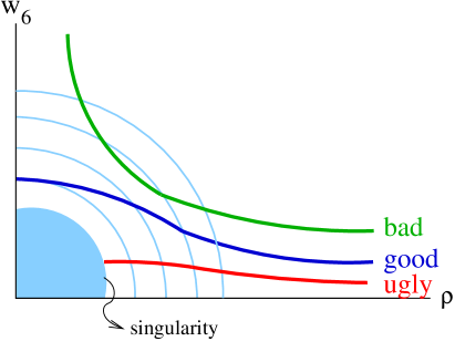
Figure 3.10: Different possibilities for solutions of the D7-brane equations of motion. The semicircles are lines of constant $r$, which should be interpreted as a scale in the dual Yang-Mills theory. The “Bad” curve cannot be interpreted as an RG flow. The other curves have an RG flow interpretation, however the infrared (small r) region of the “Ugly” curve is outside the range of validity of DBI/supergravity.

We now consider numerical solutions with the asymptotic behavior $w_{6}\sim m+c/\rho^{2}$, and find the physical solutions by imposing a regularity constraint as discussed in the previous section. Note that unlike the Euclidean AdS black hole, the Constable-Myers background has a naked singularity at $r=0$ or $\rho^{2}+w_{6}^{2}=b^{2}$. Thus there are two possibilities for a solution with an interpretation as an RG flow, which are as follows. Either the D7-brane terminates at a value of $r$ away from the naked singularity via a collapse of the $S^{3}$, or the D7-brane goes all the way to the singularity. In the latter case we would have little control over the physics without a better understanding of string theory in such highly curved backgrounds. Different possibilities for solutions of the D7-brane equations of motion are illustrated in Fig. 3.10.

Fortunately something remarkable happens. For positive values of $m$ we find that there is a discrete regular solution for each value of the mass that terminates at $w\geq 1.3$ before reaching the singularity at $w=1$. Some of these regular solutions are plotted in Fig. 3.11. For $m=0$, the solution $w_{6}=0$ is exact, which naively seems to indicate the absence of a chiral condensate $(c=0)$. However, this solution reaches the singularity, and therefore cannot be trusted. On the other hand for a very small but non-zero mass, the regular solutions require a non-vanishing $c$ and terminate before reaching the singularity! The numerical evidence (see Fig. 3.11) suggests that there is a non-zero condensate in the limit $m\rightarrow 0$.

We can study this phenomenon further in the deep infrared, in particular in view of gaining further understanding of the behaviour of the solutions shown in Fig. 3.11. Consider (3.42) as $\rho\rightarrow 0$ with $w_{6}\neq 0$ - the dilaton becomes $\rho$ independent whilst ${\cal G}\sim\rho^{3}$. Thus the potential term vanishes as $\rho^{3}$ whilst the derivative piece contains a term that behaves like $\rho^{2}\partial_{\rho}w_{6}$ and dominates. Clearly there is a solution where $w_{6}$ is just a constant. This is the regular behaviour we are numerically tuning to. It is now easy to find the flows in reverse by setting the infrared constant value of $w_{6}$ and numerically solving out to the UV. This method ensures that the flow is always regular. We have checked that the asymptotic values of the condensate as a function of mass match our previous computation at the level of a percent, showing that the numerics are under control.

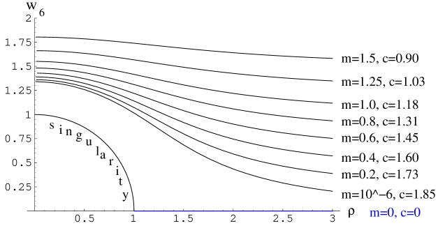
Figure 3.11: Regular solutions in the Constable-Myers background. The quark mass is measured in units of $\Lambda_{b}=1$.

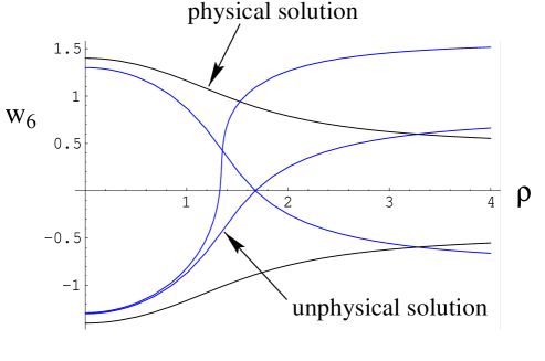
Figure 3.12: Regular D7 embedding solutions in the Constable-Myers geometry which lie close to the singularity in the infra-red.

We now realise though that there are infrared solutions where $w_{6}(\rho=0)<1.3$. These flows lie close to the singularity at $w_{6}(\rho=0)=1$ which we had hoped to exclude. Solving these flows numerically we find that they flow to negative masses in the ultraviolet. We show these flows in Fig. 3.12. Since there is a $w_{6}\rightarrow-w_{6}$ symmetry of the solution though this means there is a second regular flow for each positive mass which in the infra-red flows to negative values, also shown in Fig. 3.12. The flows that begin closer to the singularity in the infrared flow out to larger masses in the ultraviolet. This strongly suggests that these flows are not physical. When the quarks have a large mass, relative to the scale of the deformation, we do not expect the infra-red dynamics to have a large influence on the physics. Thus the flows shown in Fig. 3.11 that match onto the Karch-Katz type solution for large mass are the expected physical solutions. To find some analytic support for this conjecture we have calculated the action of two of the solutions for each mass value. The action is formally infinite if we let the flow cover the whole space. To see the difference in action we have calculated the contribution for $0<\rho<3$ only which covers the infrared part of the solution (varying the upper limit does not change the conclusions). We plot the action of the two solutions versus the quark mass in Fig. 3.13, from which it can be seen that the action for the solution lying closer to the singularity is larger. Therefore the corresponding solution is not relevant for the physics.

Figure 3.13: A plot of action vs mass for the two regular D7 embedding solutions in the Constable-Myers geometry. The higher action solutions correspond to the flows that end at $|w_{6}|<1.3$.

In a certain sense, the condensate screens the probe physics from the naked singularity. This is due to the centre of the Constable-Myers background which exerts a repulsive force on the embedded D7-brane and triggers chiral symmetry breaking. In the limit of small explicit symmetry breaking parameter $m$, any solution (or vacuum) which did not break the $U(1)$ symmetry would have $w_{6}\rightarrow 0$ for all $\rho$. If this were the case, the solution would reach the singularity (see Fig. 3.10). The screening of the singularity is reminiscent of the enhançon [156] found in ${\cal N}=2$ gravity duals - an important part of that analysis was understanding that the singularity of the geometry was screened from the physics of a D3 brane probe which led to an understanding of how the singularity could be removed. It is possible we are seeing hints of something similar, if more complicated, here, although at this stage we can not see how to remove the singular behaviour. However, since the D7-brane avoids the singularity, the existence of a singularity in the Constable-Myers background is not too bad.

3.3.2 Spontaneous $U(1)_{A}$ symmetry breaking and holographic version of the Goldstone theorem

One of the most important features of QCD dynamics is spontaneous chiral symmetry breaking by a quark condensate $\psi\tilde{\psi}$. The $U(1)$ chiral symmetry $\psi\rightarrow e^{i\theta}\psi$, $\tilde{\psi}\rightarrow e^{i\theta}\tilde{\psi}$ in the QCD-like field theory corresponds to a $U(1)$ isometry in the $w_{5}-w_{6}$ plane transverse to the D7-brane. This symmetry can be explicitly broken by a non-vanishing quark mass. In the holographic dual this corresponds to the breaking of the $U(1)$ isometry due to the separation of the D7-brane from the modified (“hairy”) D3-branes in the $w_{5}+iw_{6}$ direction, which give rise to the Constable-Myers geometry. More interesting however than an explicit breaking by a mass term is the question whether there is a spontaneous $U(1)$ chiral symmetry breaking in the case of massless quarks.

Before we can answer this question, we have to verify that the $U(1)_{A}$ symmetry is a real symmetry in a QCD-like theory with a large number of colours. Note that the $U(1)$ chiral symmetry is non-anomalous only in the limit of a large number of colours, $N_{c}\rightarrow\infty$. This can be seen in the anomaly equation of the axial $U(1)$ current $J_{\mu}=\bar{\psi}\gamma_{\mu}\gamma_{5}\psi$

$$\partial_{\mu}J^{\mu}=\frac{2N_{f}}{N_{c}}\frac{g^{2}}{16\pi^{2}}F\tilde{F}\,\,,$$ (3.44)

where $N_{f}$ is the number of flavours. For $N_{f}/N_{c}$ fixed the $U(1)$ symmetry is explicitly broken by instantons. ’t Hooft showed [157] that though the instanton term $i\theta F\tilde{F}$ is a total divergence it does not fall off fast enough at infinity to allow neglect of surface terms. The effect of the instantons is to give a mass to the $\eta^{\prime}$ meson.

The $\eta^{\prime}$ mass is given by the Witten-Veneziano formula [96, 158]

$$M^{2}_{\eta^{\prime}}=\frac{4N_{f}}{f_{\pi}^{2}}\chi_{T}\,,$$ (3.45)

where the pion decay constant, defined by $\langle 0|\bar{\psi}\gamma_{0}\gamma_{5}\psi|\pi\rangle=m_{\pi}f_{\pi}$, has experimental value 132 MeV. The topological susceptibility of the pure gauge theory, defined by

$$\chi_{T}=\frac{1}{(16\pi^{2})^{2}}\int d^{4}x\langle{\rm Tr}(F\tilde{F}(x)){\rm Tr}(F\tilde{F}(0))\rangle\,,$$ (3.46)

measures the fluctuation of the topological charge of the vacuum. Since $\chi_{T}$ is of order one and $f_{\pi}^{2}\sim N_{c}$ for large $N_{c}$, the eta-prime mass scales as $N_{f}/N_{c}$. The $\eta^{\prime}$ meson is massless in a large $N_{c}$ limit if the number of flavours $N_{f}$ is fixed. However, if $N_{f}$ scales like $N_{c}$, i.e. if $\nu=N_{f}/N_{c}$ is a fixed quantity, the $\eta^{\prime}$ meson becomes massive. This explains the experimental fact that the mass of the $\eta^{\prime}$ particle ($M_{\eta^{\prime}}=958$ MeV) is much higher than the mass of the pions (e.g. $M_{\pi^{0}}=135$ MeV), which are the Goldstone bosons of the symmetry breaking $SU(N_{f})\times SU(N_{f})\rightarrow SU(N_{f})$. However, for $N_{c}\rightarrow\infty$ with $N_{f}$ fixed, the anomaly vanishes and the $\eta^{\prime}$ becomes a real Goldstone boson [96] of a spontaneously broken $U(1)_{A}$ symmetry.

Figure 3.14: A plot of the condensate parameter $c$ vs quark mass $m$ for the regular solutions of the equation of motion in the Constable-Myers background.

In Fig. 3.14 we plot the condensate $c$ of the solutions in Fig. 3.11 as a function of the quark mass $m$. The numerics show that $c\neq 0$ for $m\rightarrow 0$. In other words the geometry spontaneously breaks the $U(1)$ chiral symmetry. This seems to be analogous to the situation in field theory, in which the path integral formally gives no spontaneous symmetry breaking, which is found only in the limit that a small explicit symmetry breaking parameter is taken to zero.

Since there is $U(1)$ chiral symmetry breaking via a condensate in the $m\rightarrow 0$ limit, we also expect there to be a Goldstone boson in the meson spectrum, which is the analogon of the $\eta^{\prime}$ particle in QCD. Such a Goldstone mode must exist as a solution to the DBI equation of motion, as the following holographic version of the Goldstone theorem shows.

Assume a D7-embedding with $w_{5}=0$ and $w_{6}\sim c/\rho^{2}$ asymptotically. A small $U(1)$ rotation $\exp(-i\epsilon)$ of $w_{5}+iw_{6}$ generates a solution with $\tilde{w}_{6}=w_{6}$ (to order $(\epsilon^{2})$) and $\tilde{w}_{5}=\epsilon c/\rho^{2}$. Thus a small fluctuation with $\delta w_{6}=0$ and $\delta w_{5}=\tilde{w}_{5}\sin(k\cdot x)$ is a normalizable solution of the linearized equations of motion,

$$f(\delta w_{5},\partial_{\rho}\delta w_{5},\partial_{x}\delta w_{5})=f(\tilde{w}_{5},\partial_{\rho}\tilde{w}_{5})+M^{2}\tilde{w}_{5}c(\rho)=0\,,$$ (3.47)

provided $M^{2}=-k^{2}=0$. Here the differential equation of the fluctuations splits into the equation of motion for $\tilde{w}_{5}$, $f(\tilde{w}_{5},\partial_{\rho}\tilde{w}_{5})=\epsilon f(w_{6},\partial_{\rho}w_{6})=0$, and a mass term with some coefficient $c(\rho)$, cf. Eq. (3.47) with the structure of Eqs. (3.24) or (3.48). In other words there must be a Goldstone boson associated with $w_{5}$ fluctuations. Note that if the embedding were asymptotically $w_{6}\sim m+c(m)/\rho^{2}$ for non-zero $m$, a $U(1)$ rotation of $w_{5}+iw_{6}$ would still generate another solution. However this solution is no longer a normalizable small fluctuation about the original embedding - asymptotically the mass will acquire a different phase moving us to a different theory. Thus if the mass is kept fixed asymptotically one does not find a massless particle in the spectrum, which reflects the explicit symmetry breaking by the quark mass $m$.

3.3.3 Meson spectrum in the Constable-Myers background

In the solutions discussed where $w_{6}$ has a background value, fluctuations in $w_{5}$ should contain the Goldstone mode. Let us turn to the numerical study of these fluctuations in the background of the $w_{6}$ solutions we have obtained above. The linearized equation of motion for small fluctuations of the form $w_{5}=f(\rho)\sin(k\cdot x)$, with $x$ the four Minkowski coordinates, are

$$\begin{array}[]{c}{d\over d\rho}\left[{e^{\phi}{\cal G}(\rho,w_{6})\over\sqrt{1+(\partial_{\rho}w_{6})^{2}}}\partial_{\rho}f(\rho)\right]+M^{2}{e^{\phi}{\cal G}(\rho,w_{6})\over\sqrt{1+(\partial_{\rho}w_{6})^{2}}}H\left({(\rho^{2}+w_{6}^{2})^{2}+b^{4}\over(\rho^{2}+w_{6}^{2})^{2}-b^{4}}\right)^{(1-\delta)/2}{(\rho^{2}+w_{6}^{2})^{2}-b^{4}\over(\rho^{2}+w_{6}^{2})^{2}}f(\rho)\\ \\ -\sqrt{1+(\partial_{\rho}w_{6})^{2}}{4b^{4}\rho^{3}\over(\rho^{2}+w_{6}^{2})^{5}}\left({(\rho^{2}+w_{6}^{2})^{2}+b^{4}\over(\rho^{2}+w_{6}^{2})^{2}-b^{4}}\right)^{\Delta/2}(2b^{4}-\Delta(\rho^{2}+w_{6}^{2})^{2})f(\rho)=0\,,\end{array}$$ (3.48)

see App. B.2 for details. The meson mass as a function of quark mass for the regular solutions for $w_{5}$ are plotted in Fig. 3.15. The meson mass indeed falls to zero as the quark mass is taken to zero providing further evidence of chiral symmetry breaking.

At small $m$, the meson mass associated to the $w_{5}$ fluctuations scales like $\sqrt{m}$ in agreement with the Gell-Mann-Oakes-Renner (GMOR) relation [159]:

$$M_{\pi}^{2}=-\frac{m\langle\bar{\psi}\psi\rangle}{N_{f}f_{\pi}^{2}}\,.$$ (3.49)

A well-known field theory argument for this scaling is as follows. The low-energy effective Lagrangian depends on a field $\eta^{\prime}$ where $\exp(i\eta^{\prime}/f)$ parameterizes the vacuum manifold and transforms by a phase under chiral $U(1)$ rotations. A quark mass term transforms by the same phase under $U(1)$ rotations, and thus breaks the $U(1)$ explicitly. A chiral Lagrangian consistent with this breaking has a term $\mu^{3}Re(m\exp(i\eta^{\prime}/f))$ where $\mu$ is some parameter with dimensions of mass. For real $m$, expanding this term to quadratic order gives a mass term $\frac{\mu^{3}}{f^{2}}m{\eta^{\prime}}^{2}$. It would be very interesting to demonstrate this scaling with $m$ analytically in the DBI/supergravity setting, along with other low-energy “theorems”. At large $m$, the meson masses scale linearly in the quark mass. This differs from the behaviour of the meson spectrum computed in the (non-supersymmetric) solitonic D4-brane background [101] which satisfies the GMOR relation to arbitrary high quark masses.

For comparison it is interesting to study $w_{6}$ fluctuations as well, which we expect to have a mass gap. Analytically linearizing the $w_{6}$ equation of motion is straightforward but the result is unrevealingly messy. Since we must eventually solve the equation numerically, we can use a simple numerical trick to obtain the solutions. We solve equation (3.42) for $w_{6}$ above but write $w_{6}=w_{6}^{0}+\delta w_{6}(r)$, where numerically we enforce $\delta w_{6}$ to be very small relative to the background configuration $w_{6}^{0}$. With this ansatz we retain the field equation in its non-linear form, but it is numerically equivalent to standard linearization. We must also add a term to the l.h.s. of (3.42) which takes into account the $x$ dependence of $\delta w_{6}$. This dependence takes the same form as that in the linearized $w_{5}$ equation (3.48), i.e. $\delta w_{6}=h(\rho)\,{\rm sin}(k\cdot x)$. The extra term to be added to (3.42) is

$$\Delta V=M^{2}{e^{\phi}{\cal G}(\rho,w_{6})\over\sqrt{1+(\partial_{\rho}w_{6})^{2}}}H\left({(\rho^{2}+w_{6}^{2})^{2}+b^{4}\over(\rho^{2}+w_{6}^{2})^{2}-b^{4}}\right)^{(1-\delta)/2}{(\rho^{2}+w_{6}^{2})^{2}-b^{4}\over(\rho^{2}+w_{6}^{2})^{2}}\delta w_{6}\,.$$ (3.50)

The numerical solutions for the $w_{6}$ fluctuations are plotted in Fig. 3.15. The $w_{6}$ fluctuations have a mass gap, as expected since they are transverse to the vacuum manifold.

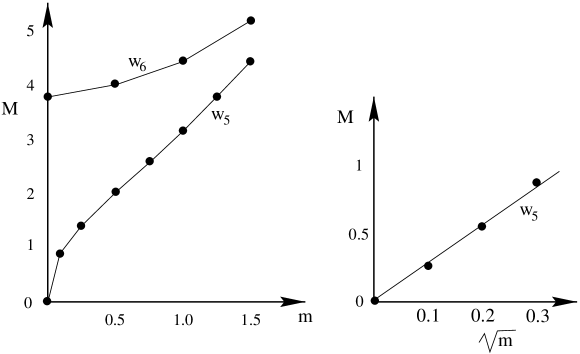
Figure 3.15: A plot of the $w_{5}$ and $w_{6}$ meson mass vs quark mass $m$ associated with the fluctuations about the regular solutions of the equation of motion for the Constable-Myers flow. The Goldstone mass is also plotted vs $\sqrt{m}$ with a linear fit.

3.3.4 Comparison with pions in QCD

Thus far we have found a particle in the spectrum which is similar to the $\eta^{\prime}$ in the large $N$ limit of QCD where it becomes a Goldstone boson. In order to obtain true pions one must have a non-abelian flavour symmetry. Unfortunately in the background which we consider, taking $N_{f}>1$ D7-branes does not give rise to a $U(N_{f})_{L}\times U(N_{f})_{R}$ chiral symmetry. Instead one gets only diagonal $U(N_{f})$ times an axial $U(1)$. The reason is that the theory contains a coupling $\tilde{\psi}_{i}X\psi_{i}$, where $i$ is a flavour index and $X$ is an adjoint scalar without any flavour indices. The coupling to $X$ explicitly breaks the $U(N_{f})_{L}\times U(N_{f})_{R}$ chiral symmetry to the diagonal subgroup, but preserves an axial $U(1)$ which acts as

$$\psi_{i}\rightarrow e^{i\theta}\psi_{i},\qquad\tilde{\psi}_{i}\rightarrow e^{i\theta}\tilde{\psi}_{i},\qquad X\rightarrow e^{-2i\theta}X.$$ (3.51)

Thus a $\tilde{\psi}_{i}\psi_{i}$ condensate will only give rise to one Goldstone boson, even if $N_{f}>1$. If $X$ were massive, there would be an approximate $U(N_{f})_{L}\times U(N_{f})_{R}$ symmetry at low energies, but this is not the case in the Constable-Myers background.

Note that $N_{f}>1$ coincident D7-branes may be embedded in the same way as a single D7-brane. In this case there are $N_{f}$ independent solutions to the linearized equations of motion for small fluctuations about this embedding, corresponding to fluctuations of the diagonal entries in a diagonal $N_{f}\times N_{f}$ matrix. These fluctuations would naively give rise to at least $N_{f}$ Goldstone bosons, rather than one. These extra states will not remain massless though since the interaction with the scalar fields which breaks the symmetry will induce a mass.

Nevertheless we can still make a rough comparison between our $\eta^{\prime}$ and QCD pions. In a two-flavour large $N$ QCD model where the quarks are degenerate one would expect four degenerate Goldstone bosons. As $N$ is decreased, instanton effects will enter to raise the $\eta^{\prime}$ mass. However since we are at large $N$, the mass formula for our Goldstone boson is applicable to the pions. It is therefore amusing to compare the Goldstone mass we predict to that of the QCD pion. There is considerable uncertainty in matching the strong coupling scale of our theory to that of QCD. In QCD the bare up or down quark mass is roughly $0.01\Lambda$ and the pion mass of order $0.5\Lambda$ (it is of course hard to know precisely what value one should pick for $\Lambda$). The comparison to our theory is a little hard to make but if we assume that $\Lambda\simeq\frac{b}{2\pi\alpha^{\prime}}=1$ then for this quark mass we find $m_{\pi}\simeq 0.25\Lambda$. The gravity dual is correctly predicting the pion mass at the level of a factor of two. Of course we cannot expect a perfect match given the additional degrees of freedom in the deformed ${\cal N}=4$ theory relative to real QCD.

4 Deconstructing extra dimensions

In the first part of this paper we have used intersecting brane configurations to study field theories with fundamental matter in the context of the AdS/CFT correspondence. In this chapter we will make use of such brane intersections in order to study some aspects of higher-dimensional field theories which describe the low-energy dynamics of intersecting M5-branes in M-theory. A description of this theory can be obtained from the low-energy effective field theory of intersecting D3-branes studied in Sec. 2.4 by a method known as deconstruction.

Deconstruction is a method to generate extra dimensions in theories with internal gauge symmetries [138, 104] (for early work on this subject, see [105, 106]). Non-renormalizable theories in $D>4$ are ill-defined above a certain cut-off at which they become strongly coupled due to a coupling constant with negative dimension. At high energies these theories require an ultraviolet completion which can frequently be provided by the deconstruction technique. This UV completion is generically a quiver theory [160] characterised by a discrete theory space, the moose or quiver diagram, which represents the field content of the theory by a lattice of sites and links. In a certain low-energy limit the quiver theory develops one or more extra dimensions and reproduces the higher-dimensional non-renormalizable theory. A peculiarity of the deconstruction approach is that the ultraviolet theory has less dimensions than the infrared theory. This is different from compactified theories which reveal their higher-dimensional behaviour at energies above the inverse radius of the compactified dimension.

In Sec. 4.1 we will review the low-energy effective field theory of D3-branes located at an orbifold singularity. This will lead us to the notion of a quiver gauge theory, an example of which with ${\cal N}=2$ supersymmetry is discussed in Sec. 4.2. In Sec. 4.3 we study the generation of extra dimensions on the Higgs branch of quiver gauge theories. We demonstrate the deconstruction of the low-energy theory of coincident M5-branes which is the six-dimensional (2, 0) superconformal theory. In Sec. 4.4 we generalize the procedure to the case of intersecting M5-branes, a brane system which is not very well understood so far. In Sec. 4.5 we will follow to some extend the fascinating idea to deconstruct M-theory itself.

4.1 D3-branes at orbifolds of the type $\mathbb{C}^{3}/\Gamma$

In this section we briefly review orbifolds of the type $\mathbb{C}^{3}/\Gamma$ with $\Gamma$ a discrete subgroup of the group $SU(4)$. We are interested in the world-volume field theory of $N|\Gamma|$ coincident D3-branes which are located at the orbifold singularity. The effect of the orbifold is to project out degrees of freedom of the four-dimensional ${\cal N}=4$ $U(N|\Gamma|)$ super Yang-Mills theory which are not invariant under the orbifold group. In general, this leads to a particular class of gauge theories known as quiver gauge theories which we will discuss in the next section.

For simplicity, let us choose for $\Gamma$ the cyclic group $\mathbb{Z}_{k}$ which acts on the three complex coordinates $z_{i}$ ($i=1,2,3$) of the transverse space $\mathbb{C}^{3}$ as

$$z_{i}\rightarrow\xi^{b_{i}}z_{i}\,,\quad$$ (4.1)

where $\xi=e^{\frac{2\pi i}{k}}$ is the generator of the group $\mathbb{Z}_{k}$ and $(b_{1},b_{2},b_{3})$ is a triple of indices.

Since the orbifold group acts on the D-brane (Chan-Paton) indices, the orbifold group $\mathbb{Z}_{k}$ is embedded into the gauge group $U(Nk)$. The invariant components of the gauge field satisfy

$$A_{\mu}=g(\xi)A_{\mu}g(\xi)^{-1}\,,$$ (4.2)

where $g(\xi)={\rm diag}({\bf 1},\xi{\bf 1},\xi^{2}{\bf 1},...,\xi^{k-1}{\bf 1})$ is the regular representation of the generator $\xi$ and ${\bf 1}$ is the unit matrix of dimension $N\times N$. The gauge field $(A_{\mu})_{ab}$ ($a,b=1,...,Nk$ color indices) is a matrix in the adjoint representation of $U(Nk)$. Since only block-diagonal matrices $A_{\mu}$ survive the projection, the gauge group is broken down to $U(N)^{k}$.

The four Weyl fermions of the ${\cal N}=4$ super Yang-Mills theory transform in the 4 of $SU(4)$. Those fermions which are invariant under the orbifold must satisfy

$$\psi^{i}=\xi^{-a_{i}}g(\xi)\psi^{i}g(\xi)^{-1}\,,$$ (4.3)

where $i=1,...,4$ and

$$a_{1}+a_{2}+a_{3}+a_{4}\equiv 0\!\!\mod k\,.$$ (4.4)

The condition (4.4) guarantees that $\Gamma$ is a subgroup of $SU(4)$ and not only of $U(4)$.

The complex scalars $\phi^{i}$, $i=1,2,3$, transform in the 6 of $SU(4)\simeq\overline{SO}(6)$, which can be obtained from the anti-symmetric tensor product of two 4’s. Invariant scalars fulfill the conditions

$$\phi^{i}=\xi^{b_{i}}g(\xi)\phi^{i}g(\xi)^{-1}\,,$$ (4.5)

where $b_{1}=a_{2}+a_{3}$, $b_{2}=a_{3}+a_{1}$, and $b_{3}=a_{1}+a_{2}$. If in addition the condition

$$b_{1}+b_{2}+b_{3}\equiv 0\!\!\mod k\,$$ (4.6)

or, equivalently, $a_{4}\equiv 0$ is satisfied, the group $\mathbb{Z}_{k}$ is embedded into $SU(3)$ and at least ${\cal N}=1$ supersymmetry is preserved.

In general, if we choose $\Gamma\subset SU(3)$ or $\Gamma\subset SU(2)$ then the ${\cal N}=4$ parent theory reduces to an ${\cal N}=1$ or ${\cal N}=2$ supersymmetric theory, respectively. If $\Gamma\subset\!\!\!\!\!\!\!\leavevmode\nobreak\ /\,\,SU(3)\subset SU(4)$ then no supersymmetry is preserved.

A simple example of a non-supersymmetric orbifold, which will be of use in Sec. 4.5 below, is $\mathbb{C}/\mathbb{Z}_{k}$ defined by the vectors

$$a_{i}=(-1,1,1,-1)\,,\quad b_{i}=(2,0,0)\,.$$ (4.7)

Since $b_{2}=b_{3}=0$ the orbifold acts only in one of the three complex planes transverse to the D3-branes while the other two planes remain flat.

4.2 Quiver gauge theories

An orbifold of the type $\mathbb{C}^{2}/\mathbb{Z}_{k}$ with ${\cal N}=2$ supersymmetry is given by the vectors

$$a_{i}=(-1,1,0,0)\,,\quad b_{i}=(1,-1,0)\,.$$ (4.8)

In this case the four fermions can be paired with the three scalars and the gauge boson to form ${\cal N}=1$ chiral and vector multiplets,

$$(\phi^{i},\psi^{i})\rightarrow\Phi^{i}\quad(i=1,2,3)\,,\quad(A_{\mu},\psi^{4})\rightarrow V\,.$$ (4.9)

In terms of these superfields the conditions (4.2)–(4.5) are given by

$$\Phi^{i}_{ab} =\xi^{a-b+b_{i}}\Phi^{i}_{ab}\,,$$ (4.10)

$$V_{ab} =\xi^{a-b}V_{ab}\,,$$ (4.11)

($a,b=1,...,k$) which have the solutions

$$\Phi^{1}=\!\begin{pmatrix}0&\Phi^{1}_{12}&0&...&0\\ 0&0&\Phi^{1}_{23}&...&0\\ \vdots&&&\ddots&\vdots\\ \vdots&&&&\Phi^{1}_{k-1,k}\\ \Phi^{1}_{k,1}&0&0&...&0\\ \end{pmatrix} ,\,\Phi^{2}=\!\begin{pmatrix}0&0&...&...&\Phi^{2}_{1,k}\\ \Phi^{2}_{21}&0&&&0\\ 0&\Phi^{2}_{23}&&&\vdots\\ \vdots&\vdots&\ddots&&\vdots\\ 0&0&...&\Phi^{2}_{k,k-1}&0\\ \end{pmatrix}$$ (4.12)

and

$$\Phi^{3}={\rm diag}(\Phi^{3}_{11},\Phi^{3}_{22},...,\Phi^{3}_{kk})\, ,\quad V={\rm diag}(V_{11},V_{22},...,V_{kk})\,.$$ (4.13)

The bifundamentals $\Phi^{1}_{i,i+1}$ and $\Phi^{2}_{i+1,i}$ transform in the

$$(1,1,...,N,\bar{N},...,1)\quad{\rm and}\quad(1,1,...,\bar{N},N,...,1)$$ (4.14)

of the gauge group $SU(N)^{k}$, while the fields $V_{ii}$ and $\Phi^{3}_{ii}$ transform in the adjoint representation.

In summary, we have the bifundamentals $\Phi^{1}_{i,i+1}$, $\Phi^{2}_{i+1,i}$, the adjoint chiral superfields $\Phi^{3}_{i}\equiv\Phi^{3}_{ii}$, and the vector superfields $V_{i}\equiv V_{ii}$. These fields can now be encoded in an oriented diagram of sites and links known as a quiver or moose diagram, as explained in the introduction, see Fig. 1.4. Each of the sites is associated with one of the $k$ $SU(N)$ gauge groups and represents a vector multiplet $V_{i}$ as well as an adjoint chiral multiplet $\Phi^{3}_{i}$ which together form a ${\cal N}=2$ vector multiplet. Two neighbouring sites are connected by two oppositely oriented links representing the complex scalars $\Phi^{1}_{i,i+1}$ and $\Phi^{2}_{i+1,i}$ which together form a ${\cal N}=2$ hyper multiplet $(\Phi^{1},{\bar{\Phi}}^{2})_{i,i+1}$.

The low-energy effective action for this quiver model is given by

$$S=\sum_{i=1}^{k}\,{\rm Tr}\int d^{4}x \left[\int d^{4}\theta\,\big{(}e^{-gV_{i+1}}\bar{\Phi}^{1}_{i+1,i}e^{gV_{i}}\Phi^{1}_{i,i+1}+e^{gV_{i+1}}\Phi^{2}_{i+1,i}e^{-gV_{i}}\bar{\Phi}^{2}_{i,i+1}\right.$$

$$+\,e^{-gV_{i}}\bar{\Phi}^{3}_{i}e^{gV_{i}}\Phi^{3}_{i}\big{)}+\frac{1}{4g^{2}}\left(\int d^{2}\theta\,\frac{1}{4}W_{i}^{\alpha}W^{i}_{\alpha}+{\rm h.c.}\right)$$

$$+ig\frac{\sqrt{2}}{3}\left.\int d^{2}\theta(\Phi^{3}_{i}\Phi^{1}_{i,i+1}\Phi^{2}_{i+1,i}-\Phi^{3}_{i+1}\Phi^{2}_{i+1,i}\Phi^{1}_{i,i+1})+{\rm h.c.}\right]$$ (4.15)

This action is obtained by substituting the solutions (4.12) and (4.13) into the ${\cal N}=4$, $d=4$ parent super Yang-Mills action. The embedding of the group $\mathbb{Z}_{k}$ into say $SU(2)_{L}$ of $SU(2)_{R}\times SU(2)_{L}\times U(1)\subset SU(4)$ breaks the R-symmetry of the parent theory down to $SU(2)_{L}\times U(1)$. The quiver theory thus describes ${\cal N}=2,d=4$ super Yang-Mills theory with gauge group $SU(N)^{k}$ which couples to $k$ bifundamental hyper multiplets.

4.3 Deconstruction of the M5-brane action

In the last section we have derived the low-energy theory of a stack of $kN$ D3-branes at an orbifold of the type $\mathbb{C}^{2}/\mathbb{Z}_{k}$. The action (4.2) of this four-dimensional quiver theory is the starting point for the deconstruction of the M5-brane theory. We will show that on the Higgs branch of the quiver gauge theory two extra dimensions are generated and the theory becomes equivalent to the six-dimensional (2, 0) theory.

4.3.1 Deconstruction of extra dimensions

We start by considering a particular Higgs branch of the quiver theory (4.2) on which the scalars in all hyper multiplets have the same expectation value, i.e.

$$\langle\phi^{1}_{i,i+1}\rangle=\langle\phi^{2}_{i+1,i}\rangle=v\bf{1}\,,$$ (4.16)

independent of $i$. This causes the breakdown of the gauge group $SU(N)^{k}$ to its diagonal subgroup $SU(N)$ leading to massive gauge bosons $A_{i}^{\mu}$. To see this, we consider the kinetic term for the scalars $\phi^{1}_{i,i+1}$ of the bifundamentals $\Phi^{1}_{i,i+1}$ (analogous for $\Phi^{2}_{i+1,i}$) which is given by

$${\rm Tr}\left((D_{\mu}\phi^{1}_{i,i+1})^{\dagger}D^{\mu}\phi^{1}_{i,i+1}\right)\subset{\rm Tr}\left(e^{-gV_{i+1}}\bar{\Phi}^{1}_{i+1,i}e^{gV_{i}}\Phi^{1}_{i,i+1}\right)\,,$$ (4.17)

where the covariant derivative is $D_{\mu}\phi^{1}_{i,i+1}\equiv\partial_{\mu}\phi^{1}_{i,i+1}-gA^{i}_{\mu}\phi^{1}_{i,i+1}-g\phi^{1}_{i,i+1}A^{i+1}_{\mu}$. Substituting the VEVs $\langle\phi^{1}_{i,i+1}\rangle=v{\bf 1}$ into the Lagrangian, the term (4.17) reduces to

$$g^{2}v^{2}(A_{i}^{\mu}-A_{i+1}^{\mu})^{2} =g^{2}v^{2}\left[2(A_{i}^{\mu})^{2}-A_{i-1}^{\mu}A_{i}^{\mu}-A_{i+1}^{\mu}A_{i}^{\mu}\right]=\frac{1}{2}A_{i\mu}M^{2}A_{j}{}^{\mu}\,,$$ (4.18)

where we defined the mass matrix $M^{2}$ by

$$M^{2}\equiv 2g^{2}v^{2}\begin{pmatrix}2&-1&&&-1\\ -1&2&-1&&&\\ &\ddots&\ddots&\ddots\\ &&-1&2&-1\\ -1&&&-1&2\end{pmatrix}\,.$$ (4.19)

The eigenvalues of $M$ turn out to be [22]

$$m_{l}=2\sqrt{2}gv\sin\frac{l\pi}{k}\,,\quad 0\leq l\leq k-1\,.$$ (4.20)

For large $k$ (and small $l$) the mass spectrum becomes linear, $m_{l}\approx 2\sqrt{2}gv\frac{l\pi}{k}$ and approximates a Kaluza-Klein tower of states corresponding to the compactification of a fifth dimension. Comparing (4.20) with the conventional expression of a Kaluza-Klein spectrum, $m_{l}=l/R_{5}$, we find

$$2\pi R_{5}=\frac{k}{\sqrt{2}gv}\,$$ (4.21)

for the radius $R_{5}$ of the compact dimension.

This spectrum was expected since the action (4.2) looks like a latticized five-dimensional theory, where only the fifth dimension is discritized on a spatial circle. The quiver diagram in Fig. 1.4, which encodes the field content of the theory, visualizes the discretization of the extra dimension. As $k\rightarrow\infty$ the indices of the fields turn into continuous labels parameterizing the extra dimension. For instance, the discrete index $i$ of the four-dimensional gauge bosons $A_{\mu}^{i}(x)$ becomes a continuous label $z$, i.e. $A_{\mu}^{i}\rightarrow A_{\mu}(x,z)$ yielding four components of a five-dimensional gauge boson $A_{M}(x,z)$ ($M=0,1,2,3,4$). Its fifth component $A_{4}$ is given by the imaginary part of $\phi_{i,i+1}$.

Dyonic excitations

The Kaluza-Klein spectrum of massive gauge bosons shows the occurrence of a fifth dimension on the Higgs branch. The deconstructed theory is however not just a five-dimensional gauge theory. Surprisingly, there exists a further Kaluza-Klein spectrum of magnetic excitations indicating the deconstruction of a second extra dimension. Due to the conformal invariance of the quiver theory, which is inherited from the ${\cal N}=4$ parent theory, the theory possesses an $SL(2,\mathbb{Z})$ S-duality. Substituting $g\rightarrow k/g$ in (4.20), we obtain the magnetic mass spectrum

$$M_{l}=2\sqrt{2}\frac{kv}{g}\sin\frac{l\pi}{k}\,,\quad 0\leq l\leq k-1\,.$$ (4.22)

As above, for small $l$ this approximates a KK spectrum which generates a sixth dimension of circumference

$$2\pi R_{6}=\frac{g}{\sqrt{2}v}\,.$$ (4.23)

Figure 4.1: Deconstruction of extra dimensions at low energies.

In summary, on the Higgs branch the quiver theory develops two extra dimensions corresponding to the two cycles of a torus with radii $R_{5}$ and $R_{6}$. Kaluza-Klein modes with momenta in both directions are dyons in the quiver theory. The higher-dimensional behaviour of the quiver theory at low energies is shown schematically in Fig. 4.1. The inverse of the lattice spacing $a=1/(\sqrt{2}gv)$ plays the role of a cut-off. For finite $a$ the theory is six-dimensional up to the cut-off $a^{-1}$ above which the theory is still well-defined but lacks six-dimensional Lorentz invariance. In the continuum limit $g,v\rightarrow\infty$ keeping $R_{5}$ and $R_{6}$ fixed the lattice spacing $a$ and the theory becomes six-dimensional to arbitrary high dimensions.

4.3.2 String theory analysis

We now show that the Higgs branch theory of the quiver model (4.2) is the six-dimensional (2, 0) theory compactified on a torus which is the world-volume theory of wrapped M5-branes. To see this we will make use of string theory dualities in the orbifold realisation of the quiver theory.

Figure 4.2: The orbifold $\mathbb{C}^{2}/\mathbb{Z}_{k}$ for $k=5$.

Fig. 4.2 shows the covering space of the orbifold $\mathbb{C}^{2}/\mathbb{Z}_{k}$ (for $k=5$) and the location of a stack of $N$ D3-branes and their mirror branes. The Higgs branch of the quiver gauge theory is parameterized by the VEVs $v$ of the bifundamentals, i.e. the D3-branes are located some distance $d\sim v$ away from the orbifold singularity. The KK states in the field theory descend from fundamental strings and D-strings stretching between the D-branes and its mirror branes.

The first issue to verify is the doubling of supersymmetry on the Higgs branch. While the ${\cal N}=2$ quiver gauge theory has 8 supercharges at high energies, we expect it to have 16 supercharges at low energies, where it is supposed to turn into the M5-brane theory. The amount of supersymmetry is effectively enhanced by a factor two.

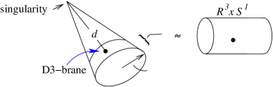
Figure 4.3: Far away from the orbifold singularity the cone can be approximated locally by a cylinder.

$R_{S^{1}}=d/k$

This can be understood from a geometrical point of view as follows. The orbifold $\mathbb{C}^{2}/\mathbb{Z}_{k}$ can be introduced in the six-dimensional transverse space of the D3-branes with flat metric $ds^{2}=dz_{i}d\bar{z}_{i}$ ($i=1,2,3$) by redefining the coordinates,

$$z_{1}=r_{1}exp(i\theta+i\phi/k)\,,\quad z_{2}=r_{2}exp(i\theta-i\phi/k)\,,\quad z_{3}\,\,\textmd{unchanged}\,$$ (4.24)

with ranges $\phi,\theta\in(0,2\pi)$. Expanding $r_{1}=d/\sqrt{2}+x_{1}$, $r_{2}=d/\sqrt{2}+x_{2}$, $\theta=x_{3}/d$ the metric becomes

$$ds^{2}=dz_{3}d\bar{z}_{3}+dx_{1}^{2}+dx_{2}^{2}+dx_{3}^{2}+\frac{d^{2}}{k^{2}}d\phi^{2}$$ (4.25)

plus corrections proportional to $1/k$ which vanish in the large $k$ limit. The metric shows that away from the singularity the orbifold geometry $\mathbb{C}^{2}/\mathbb{Z}_{k}$ degenerates into a cylinder, $\mathbb{R}^{3}\times S^{1}$, where the radius of the $S^{1}$ is given by $R_{S^{1}}=l^{2}_{s}/R_{5}$ with $R_{5}\equiv kl^{2}_{s}/d$, see Fig. 4.3. The D3-branes are effectively located in a flat geometry, far away from the highly curved region close to the orbifold singularity at the tip of the cone. Recall that the effect of the orbifold was to break supersymmetry by a half. Now in the locally flat region of the orbifold the supersymmetry of the effective D-brane theory is doubled.

In the decoupling limit $g_{s}$ fixed, $l_{s}\rightarrow 0$ the radius $R_{S^{1}}$ becomes sub-stringy. A more appropriate description is obtained by T-dualizing the D3-branes to D4-branes which wrap around the T-dual $S^{1}$ with large radius $R_{5}$. However, the type IIA string coupling $g_{s}^{\prime}=g_{s}R_{5}/l_{s}$ becomes very large for $l_{s}\rightarrow 0$ such that we have to lift the D4-branes to M5-branes in M-theory. These M5-branes wrap a two-torus with radii $R_{5}$ and $R_{6}=g_{s}^{\prime}l_{s}=g_{s}R_{5}$. The eleven-dimensional Planck length $l_{p}^{3}=l_{s}^{3}g_{s}^{\prime}=l_{s}^{2}R_{6}$ goes to zero for $l_{s}\rightarrow 0$. The world-volume theory of the D3-branes at $\mathbb{C}^{2}/\mathbb{Z}_{k}$ therefore turns on the Higgs branch into the world-volume theory of M5-branes wrapped around a two-torus.

To conclude, taking the number $k$ of nodes in the quiver diagram to infinity, the Higgs branch of the 4D ${\cal N}=2$ orbifold theory is equivalent to the 6D ${\cal N}=(2,0)$ gauge theory compactified on a torus. The gauge group is thereby broken down to its diagonal subgroup, $SU(N)^{k}\rightarrow SU(N)$ and supersymmetry is enhanced from eight to sixteen supercharges.

4.4 Intersecting M5-branes

In this section we discuss the low energy dynamics of orthogonally intersecting M5-branes which are not very well understood by now. In addition to a non-abelian chiral two-form, this theory has tensionless strings localized at the intersection corresponding to M2-branes stretched between the M5-branes [162]. These tensionless strings are in some sense fundamental, as they are not excitations of a chiral two-form. The only known formulation of the M5-M5 intersection is the DLCQ M(atrix) description proposed in [163].

Here we shall present the (de)construction of the M5-M5 intersection, which is a natural extension of the (de)construction of parallel M5-branes discussed in the last section. This will be accomplished by taking a $k\rightarrow\infty$ limit of the theory describing intersecting D3-branes at a $\mathbb{C}^{2}/\mathbb{Z}_{k}$ orbifold. At a certain point in the moduli space, two compact latticized extra dimensions are generated. In an appropriate $k\rightarrow\infty$ limit, we expect that the extra directions become continuous, such that the intersection of four-dimensional world-volumes over $1+1$ dimensions becomes an intersection of six-dimensional world-volumes over $1+3$ dimensions.

The infrared dynamics of the D3-D3 intersection at a $\mathbb{C}^{2}/\mathbb{Z}_{k}$ orbifold is described by a defect conformal field theory with two-dimensional $(4,0)$ supersymmetry. This theory belongs to the class of conformal field theories with defects which we studied in Ch. 2. The action of this $(4,0)$ theory is readily constructed in $(2,0)$ superspace, starting from the action for the D3-D3 intersection in flat space which we constructed in Sec. 2.4.2. The field content of the $(4,0)$ theory is summarized by a quiver (or “moose”) diagram consisting of two concentric rings, and spokes stretching between the inner and outer rings. For large $k$ this gives rise to a discretized version of the field theory corresponding to the low-energy limit of the M5-M5 intersection. The spokes in the quiver diagram will be seen to correspond to strings localized at the M5-brane intersection.

Moreover, we examine the relation between the moduli space of vacua of the $(4,0)$ defect conformal field theory and that of the M5-M5 intersection. On a particular part of the Higgs branch of the defect CFT, the resolution of the intersection to a holomorphic curve $xy=c$ can be seen very explicitly from F-flatness conditions. This point in the Higgs branch corresponds to a vacuum of the M5-M5 theory in which tensionless strings have condensed. By going to another point on the Higgs branch of the defect CFT for which the string tension in the M5-M5 theory is non-zero, we will be able to match the $SU(2)_{L}$ R-symmetry of the $(4,0)$ theory with the $SU(2)$ R-symmetry of the M5-M5 intersection, which has ${\cal N}=2,d=4$ supersymmetry.

4.4.1 D3-D3 intersection at a $\mathbb{C}^{2}/\mathbb{Z}_{k}$ orbifold

To (de)construct the theory of the M5-M5 intersection, we shall consider a pair of intersecting stacks of D3-branes at an $\mathbb{C}^{2}/\mathbb{Z}_{k}$ orbifold point. One set of D3-branes is located at $X^{4,5,6,7,8,9}=0$ while the other set of ${\rm D3}^{\prime}$-branes is located at $X^{2,3,6,7,8,9}=0$. The $\mathbb{C}^{2}/\mathbb{Z}_{k}$ is spanned by the coordinates $u=X^{6}+iX^{7}$ and $w=X^{8}+iX^{9}$ subject to the orbifold condition $u\sim\xi u,w\sim\xi^{-1}w$ where $\xi=\exp(2\pi i/k)$. Before orbifolding, the theory of intersecting D3-branes has $(4,4)$ supersymmetry with an $SU(2)_{L}\times SU(2)_{R}$ R-symmetry. The $SU(2)_{L}\times SU(2)_{R}$ component of the R-symmetry acts as an $SO(4)$ transformation on the real components of $u$ and $w$, which are the coordinates $X^{6,7,8,9}$. The orbifold breaks $SU(2)_{L}\times SU(2)_{R}$ to $SU(2)_{L}$, under which the pair ($u,w^{*}$) transforms as a doublet. Moreover, the supersymmetry is broken from $(4,4)$ to $(4,0)$. It is interesting to observe that the theory is chiral.

Orbifold projection

The Lagrangian describing the D3-D3 intersection in the $\mathbb{C}^{2}/\mathbb{Z}_{k}$ orbifold can be obtained from the action of the D3-D3 intersection in flat space given in (2.4.2) - (2.70). Following Refs. [160, 164] we start with $Nk$ D3-branes intersecting $N^{\prime}k$ D3-branes in a flat background and project out the degrees of freedom which are not invariant under the $\mathbb{Z}_{k}$ orbifold group, which is generated by a combination of a gauge symmetry and an R-symmetry. An important constraint on the orbifold action is that the theory on each stack of D3 branes (ignoring strings connected to the other stack) should be the ${\cal N}=2,d=4$ super Yang-Mills theory described by the quiver in Fig. 1.4 (in Ch. 1), with gauge group $SU(N)^{k}$ or $SU(N^{\prime})^{k}$.

The orbifold action which gives the quiver of Fig. 1.4 for both the D3 and the D3^′ degrees of freedom separately, and breaks the $SU(2)_{L}\times SU(2)_{R}$ R-symmetry to $SU(2)_{L}$ is as follows. The embedding of the $\mathbb{Z}_{k}$ orbifold group in the $U(Nk)$ and $U(N^{\prime}k)$ gauge groups is given by

$$g(\xi) =\begin{pmatrix}I_{N\times N}&&&\\ &\xi I_{N\times N}&&\\ &&\xi^{2}I_{N\times N}&\\ &&&\ddots\end{pmatrix}\,,$$ (4.26)

$$g^{\prime}(\xi) =\begin{pmatrix}I_{N^{\prime}\times N^{\prime}}&&&\\ &\xi I_{N^{\prime}\times N^{\prime}}&&\\ &&\xi^{2}I_{N^{\prime}\times N^{\prime}}&\\ &&&\ddots\end{pmatrix}\,,$$ (4.27)

where $\xi$ is the generator $\exp(2\pi i/k)$ of $\mathbb{Z}_{k}$. The embedding of the $\mathbb{Z}_{k}$ orbifold group in the R-symmetry is given by

$$h(\xi)=e^{i\pi\sigma^{3}/k}\,,$$ (4.28)

where $h$ belongs to $SU(2)_{R}$. The field theory describing the D3-D$3^{\prime}$ intersection at the orbifold is then obtained from that of the D3-D$3^{\prime}$ intersection in flat space by projecting out fields which are not invariant under the orbifold action. The result is an $SU(N)^{k}\times SU(N^{\prime})^{k}$ gauge theory with $(4,0)$ supersymmetry and $SU(2)_{L}\times U(1)$ R-symmetry.

In $(2,2)$ superspace, the orbifold acts on superspace coordinates as

$$\theta^{-}\rightarrow\xi\theta^{-}\,,$$ (4.29)

but trivially on $\theta^{+}$. On the $(2,2)$ superfields the orbifold acts as

$${\rm D3}: V\rightarrow g(\xi)Vg^{\dagger}(\xi)\,, \Sigma\rightarrow\xi^{-1}g(\xi)\Sigma g^{\dagger}(\xi)\,,$$

$$Q_{1}\rightarrow\xi g(\xi)Q_{1}g^{\dagger}(\xi)\,, Q_{2}\rightarrow g(\xi)Q_{2}g^{\dagger}(\xi)\,,$$

$$\Phi\rightarrow g(\xi)\Phi g^{\dagger}(\xi)\,,$$

$${\rm D3}^{\prime}: {\cal V}\rightarrow g^{\prime}(\xi){\cal V}g^{\prime\dagger}(\xi)\,, \Omega\rightarrow\xi^{-1}g^{\prime}(\xi)\Omega g^{\prime\dagger}(\xi)\,,$$

$$S_{1}\rightarrow\xi g^{\prime}(\xi)S_{1}g^{\prime\dagger}(\xi)\,, S_{2}\rightarrow g^{\prime}(\xi)S_{2}g^{\prime\dagger}(\xi)\,,$$

$$\Upsilon\rightarrow g^{\prime}(\xi)\Upsilon g^{\prime\dagger}(\xi)\,,$$

$${\rm D3-D3^{\prime}}: B\rightarrow g(\xi)Bg^{\prime\dagger}(\xi)\,, \tilde{B}\rightarrow g^{\prime}(\xi)\tilde{B}g^{\dagger}(\xi)\,,$$ (4.30)

with $g$, $g^{\prime}$ as in (4.26), (4.27). Starting with the action (2.4.2) - (2.70) and projecting out the degrees of freedom which are not invariant under (4.30) will give a $(4,0)$ supersymmetric action with manifest $(2,0)$ supersymmetry.

To illustrate how the orbifold acts on components, we consider the action (4.30) on the $(2,2)$ twisted superfield $\Sigma$. On the bosonic components, this corresponds to

$$\sigma \sim\xi^{-1}g(\xi)\sigma g^{\dagger}(\xi)\,,\quad F_{01}\sim g(\xi)F_{01}g^{\dagger}(\xi)\,.$$ (4.31)

This is consistent with the fact that the field $\sigma$ characterises fluctuations transverse to both D3-branes, i.e. fluctuations in the orbifold directions. This field is naturally associated with fluctuations in the $w=X^{8}+iX^{9}$ directions which satisfy the orbifold condition $w\sim\xi^{-1}w$. Upon projecting out the parts which are not invariant under the orbifold, $\sigma$ becomes a set of $k$ bifundamentals in the representations $(\cdots N,\bar{N},\cdots)$ of $SU(N)^{k}$. These bifundamental fields are written as $\sigma_{j,j+1}$, where $j=1\cdots k$ and the first(second) index labels the gauge group with respect to which the field is a fundamental (anti-fundamental). Fields which are adjoints with respect to one of the factors will be written with a single index.

Quiver action in two-dimensional $(2,0)$ superspace

Since the $(4,4)$ supersymmetry of the action (2.4.2) - (2.70) is broken down to $(4,0)$ by the orbifold, an adequate formulation of the corresponding quiver gauge theory is best given in $(2,0)$ superspace. In order to project out the degrees of freedom which are not invariant under the orbifold, we rewrite the parent action using manifest $(2,0)$ supersymmetry. To this end, we decompose the $(2,2)$ superfields under $(2,0)$ supersymmetry. The decomposition of the $(2,2)$ superfields is as follows (see for instance [143, 165]):

i) $(2,2)$ vector $\rightarrow$ $(2,0)$ vector $+$ $(2,0)$ chiral,

ii) $(2,2)$ chiral $\rightarrow$ $(2,0)$ chiral $+$ $(2,0)$ Fermi.

These $(2,0)$ superfields have the following component decomposition:

i) $(2,0)$ vector superfield $V$: two gauge connections $A_{0},A_{1}$ and one fermion $\chi_{-}$,

ii) $(2,0)$ chiral superfields $\Phi$: one complex scalar $\phi$ and a fermion $\psi_{+}$,

iii) $(2,0)$ Fermi superfields $\Lambda$: one chiral fermion $\lambda_{-}$. The full expansion of this anticommuting superfield contains an auxiliary field and a holomorphic function of $(2,0)$ chiral superfields.

For the theory given by the action (2.4.2) - (2.70), the decomposition of the $(2,2)$ superfields of the D3-D3 intersection in flat space gives the following $(2,0)$ superfields (we shall henceforward write $(2,2)$ superfields in boldface):

$${\rm D3}: {\bf Q}_{1}\rightarrow Q_{1},\Lambda^{Q_{1}}, {\bf Q}_{2}\rightarrow Q_{2},\Lambda^{Q_{2}}, {\bf\Phi}\rightarrow\Phi,\Lambda^{\Phi}, {\bf V}\rightarrow V,\Theta_{V}\,,$$

$${\rm D3}^{\prime}: {\bf S}_{1}\rightarrow S_{1},\Lambda^{S_{1}}, {\bf S}_{2}\rightarrow S_{2},\Lambda^{S_{2}}\,, {\bf\Upsilon}\rightarrow\Upsilon,\Lambda^{\Upsilon}, {\bf{\cal V}}\rightarrow{\cal V},\Theta_{\cal V}\,,$$

$${\rm D3}-{\rm D3}: {\bf B}\rightarrow B,\Lambda^{B}, \tilde{\bf B}\rightarrow\tilde{B},\Lambda^{\tilde{B}}\,.$$ (4.32)

Since we wish to obtain the action for the D3-D3 intersection at the $\mathbb{C}^{2}/\mathbb{Z}_{k}$ singularity in $(2,0)$ superspace, we write the orbifold action (4.29), (4.30) in $(2,0)$ superspace. In terms of the $(2,0)$ decomposition, the orbifold acts as follows:

$${\rm D3}: Q_{1}\rightarrow\xi g(\xi)Q_{1}g^{\dagger}(\xi)\,,\quad \Lambda^{Q_{1}}\rightarrow g(\xi)\Lambda^{Q_{1}}g^{\dagger}(\xi)\,,$$

$$Q_{2}\rightarrow g(\xi)Q_{2}g^{\dagger}(\xi)\,,\quad \Lambda^{Q_{2}}\rightarrow\xi^{-1}g(\xi)\Lambda^{Q_{2}}g^{\dagger}(\xi)\,,$$

$$\Phi\rightarrow g(\xi)\Phi g^{\dagger}(\xi)\,,\quad \Lambda^{\Phi}\rightarrow\xi^{-1}g(\xi)\Lambda^{\Phi}g^{\dagger}(\xi)\,,$$

$$V\rightarrow g(\xi)Vg^{\dagger}(\xi)\,,\quad \Theta_{V}\rightarrow\xi^{-1}g(\xi)\Theta_{V}g^{\dagger}(\xi)\,,$$

$${\rm D3}^{\prime}: S_{1}\rightarrow\xi g^{\prime}(\xi)S_{1}g^{\prime\dagger}(\xi)\,,\quad \Lambda^{S_{1}}\rightarrow g^{\prime}(\xi)\Lambda^{S_{1}}g^{\prime\dagger}(\xi)\,,$$

$$S_{2}\rightarrow g^{\prime}(\xi)S_{2}g^{\prime\dagger}(\xi)\,,\quad \Lambda^{S_{2}}\rightarrow\xi^{-1}g^{\prime}(\xi)\Lambda^{S_{2}}g^{\prime\dagger}(\xi)\,,$$

$$\Upsilon\rightarrow g^{\prime}(\xi)\Upsilon g^{\prime\dagger}(\xi)\,,\quad \Lambda^{\Upsilon}\rightarrow\xi^{-1}g^{\prime}(\xi)\Lambda^{\Upsilon}g^{\prime\dagger}(\xi)\,,$$

$${\cal V}\rightarrow g^{\prime}(\xi){\cal V}g^{\prime\dagger}(\xi)\,,\quad \Theta_{\cal V}\rightarrow\xi^{-1}g^{\prime}(\xi)\Theta_{\cal V}g^{\prime\dagger}(\xi)\,,$$

$${\rm D3}-{\rm D3}^{\prime}: B\rightarrow g(\xi)Bg^{\prime}{}^{\dagger}(\xi)\,,\quad \Lambda^{B}\rightarrow\xi^{-1}g(\xi)\Lambda^{B}g^{\prime}{}^{\dagger}(\xi)\,,\quad$$

$$\tilde{B}\rightarrow g^{\prime}(\xi)\tilde{B}g{}^{\dagger}(\xi)\,,\quad \Lambda^{\tilde{B}}\rightarrow\xi^{-1}g^{\prime}(\xi)\Lambda^{\tilde{B}}g^{\dagger}(\xi)\,.$$ (4.33)

Each component of a $(2,0)$ superfield transforms under the orbifold action in the same way as the $(2,0)$ superfield itself. Note that this was not the case for $(2,2)$ superfields. The degrees of freedom which are invariant under (4.4) together with their $SU(N)^{k}\times SU(N^{\prime})^{k}$ gauge transformation properties are summarized by the quiver diagram in Fig. 4.4. The quiver consists of an inner and an outer ring. Each of them is equivalent to the quiver diagram shown in Fig. 1.4 which provides the field content for the (de)construction of the six-dimensional $(2,0)$ superconformal field theory. We will see below that the spokes in the diagram, which connect both rings, represent the degrees of freedom for the (de)construction of a ${\cal N}=2,d=4$ field theory located at the M5-M5 intersection.

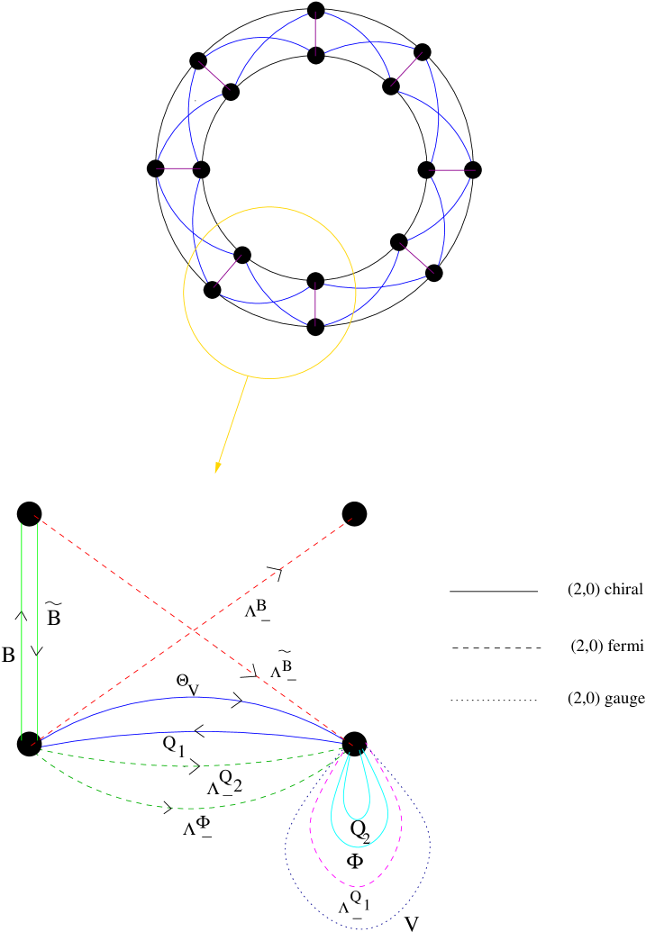
Figure 4.4: Quiver diagram for intersecting D3-branes at a $\mathbb{C}^{2}/\mathbb{Z}_{k}$ orbifold (with $k$=8). The nodes of the inner and outer circle are associated with the $SU(N^{\prime})^{k}$ and $SU(N)^{k}$ gauge groups respectively. The parts which have not been drawn in the detailed “close-up” are easily inferred from the $\mathbb{Z}_{k}$ symmetry and by swapping D3 degrees of freedom with D$3^{\prime}$ degrees of freedom.

We do not need the full action of the $(4,0)$ quiver theory. For now we just give the $(2,0)$ term analogous to a superpotential, which will be all that we require for most purposes. Superpotentials of $(2,0)$ theories have the generic structure

$$W=\int d\theta^{+}\sum_{a}\Lambda^{a}J_{a}(\Phi_{i})|_{\theta^{+}=0}\,,$$ (4.34)

where $J_{a}(\Phi_{i})$ is a holomorphic function of the chiral superfields. For the D3-D3 intersection at a $\mathbb{C}^{2}/\mathbb{Z}_{k}$ orbifold, this term descends from the superpotential of the D3-D3 intersection in flat space which is presented in $(2,0)$ superspace in App. C.2. Upon projecting out the degrees of freedom which are not invariant under the orbifold (4.4), one obtains the $(2,0)$ superpotential

$$W=W_{\rm D3}+W_{\rm D3^{\prime}}+W_{\rm D3-D3^{\prime}}\,,$$ (4.35)

where

$$W_{\rm D3}=\int d^{2}xd\theta^{+}{\rm tr}_{N\times N} \left(g\Lambda^{\Phi}_{j,j+1}(Q^{2}_{j+1}Q^{1}_{j+1,j}\,-\,Q^{1}_{j+1,j}Q^{2}_{j})\right.$$ (4.36)

$$+ \,\Lambda^{Q^{1}}_{j}[\partial_{\bar{x}}+g\Phi_{j},Q^{2}_{j}]$$

$$+ \,\left.\left.\Lambda^{Q^{2}}_{j,j+1}(-\partial_{\bar{x}}Q^{1}_{j+1,j}-gQ^{1}_{j+1,j}\Phi_{j}+g\Phi_{j+1}Q^{1}_{j+1,j})\right)\right|_{\bar{\theta}^{+}=0}\,,$$

$$W_{\rm D3^{\prime}}=\int d^{2}yd\theta^{+}{\rm tr}_{N^{\prime}\times N^{\prime}} \left(g\Lambda^{\Upsilon}_{j,j+1}(S^{2}_{j+1}S^{1}_{j+1,j}\,-\,S^{1}_{j+1,j}S^{2}_{j})\right.$$ (4.37)

$$+ \,\Lambda^{S^{1}}_{j}[\partial_{\bar{x}}+g\Upsilon_{j},S^{2}_{j}]$$

$$+ \,\left.\left.\Lambda^{S^{2}}_{j,j+1}(-\partial_{\bar{x}}S^{1}_{j+1,j}-gS^{1}_{j+1,j}\Upsilon_{j}+g\Upsilon_{j+1}S^{1}_{j+1,j})\right)\right|_{\bar{\theta}^{+}=0}\,,$$

$$W_{\rm D3-D3^{\prime}}=g\int d\theta^{+}{\rm tr}_{N\times N} \left(\Lambda^{B}_{j,j+1}(\tilde{B}_{j+1}Q^{1}_{j,j+1}-S^{1}_{j+1,j}\tilde{B}_{j})+\Lambda^{Q^{1}}_{j}B_{j}\tilde{B}_{j}\right)$$ (4.38)

$$+{\rm tr}_{N^{\prime}\times N^{\prime}} \left.\left(\Lambda^{\tilde{B}}_{j,j+1}(Q^{1}_{j+1,j}B_{j}-B_{j+1}S^{1}_{j+1,j})-\Lambda^{S^{1}}_{j}\tilde{B}_{j}B_{j}\right)\right|_{\bar{\theta}^{+}=0}\,.$$

In order to see that this theory has indeed $(4,0)$ supersymmetry, we record the basic structure of the $(4,0)$ multiplets which appear. These are as follows:

• $(4,0)$ hypermultiplets composed of two $(2,0)$ chiral multiplets: There are five multiplets of this type containing the pairs $(B,\tilde{B}),(\Phi,Q_{2}),(\Theta_{V},Q_{1}),(\Upsilon,S_{2})$ and $(\Theta_{\cal V},S_{1})$.

• $(4,0)$ vector multiplets composed of one $(2,0)$ vector multiplet and one $(2,0)$ Fermi multiplet: There are two multiplets of this type containing the pairs $(V,\Lambda^{Q_{1}})$ and $({\cal V},\Lambda^{S_{1}})$.

• $(4,0)$ Fermi multiplets composed of one $(2,0)$ Fermi multiplet: There are six multiplets of this type corresponding to the $(2,0)$ Fermi multiplets $\Lambda^{B}$, $\Lambda^{\tilde{B}}$, $\Lambda^{\Phi}$, $\Lambda^{Q_{2}}$, $\Lambda^{\Upsilon}$ and $\Lambda^{S_{2}}$.

The transformation properties under the $(4,0)$ $SU(2)_{L}$ R-symmetry are readily obtained from Tab. 2.2 on page 2.2. Note that the $SU(2)_{L}$ R-symmetry acts on the degrees of freedom of either the inner or outer ring of the quiver diagram as the $SU(2)$ R-symmetry of the associated ${\cal N}=2,d=4$ theory.

In the following section, we shall make use of this superpotential to discuss the (de)construction of the M5-M5 intersection.

4.4.2 (De)constructing the M5-M5 intersection

The inner and outer circle of the quiver diagram in Fig. 4.4 are each separately equivalent to the quiver diagram of Fig. 1.4, which (de)constructs the $(2,0)$ theory upon taking the appropriate large $k$ limit [113]. The new twist here is that there are degrees of freedom connecting the inner and outer rings. These are localized at the intersection of the D3-branes, and it is natural to expect that in the large $k$ limit, these correspond to the tensionless strings localized at the intersection of M5-branes. One reason to expect this follows from a trivial extension of an argument given in [113] based on the IIB string theory embedding. As discussed in Sec. 4.3.2, in the $k\rightarrow\infty$ limit, the $\mathbb{C}^{2}/\mathbb{Z}_{k}$ orbifold appears as a flat $S^{1}\times\mathbb{R}^{3}$ geometry sufficiently far away from the orbifold point (or sufficiently far out on the Higgs branch). For intersecting D3-branes, T-dualizing and lifting to M-theory on this space gives rise to intersecting M5-branes wrapping a torus of fixed dimensions. The strings stretched between the orthogonal D3-branes then become membranes stretched between M5-branes, as shown in Fig. 4.5. In the following, we shall focus on the field theoretic origins of the tensionless strings at the intersection.

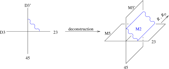
Figure 4.5: (De)construction of two extra dimensions along the torus with radii $R_{5}$ and $R_{6}$. The common directions $x^{0}$ and $x^{1}$ as well as the four orbifold directions are suppressed.

(De)constructing the $(2,0)$ theory

Before discussing the strings localized at the intersection, we shall briefly review the field theoretic arguments behind the (de)construction of the six-dimensional $(2,0)$ theory discovered in [113]. The quiver diagram of the deconstructed theory is that of Fig. 1.4, which describes a superconformal ${\cal N}=2,d=4$ gauge theory with gauge group $SU(N)^{k}$. The hypermultiplets described by the double lines stretched between adjacent nodes contain two complex scalars in bifundamental representations. The quiver diagram can be viewed as a discretization of an extra circular spatial dimension if one takes all the bifundamental scalars to have the same non-zero expectation value. At this point on the Higgs branch the gauge symmetry is broken from $SU(N)^{k}$ to the diagonal $SU(N)$.

To make closer contact with our work, we show how the extra dimensions arise from the ${\cal N}=2,d=4$ theory using the language of two-dimensional $(2,0)$ superspace. Consider the term $W_{\rm D3}$ in the superpotential (4.35), which involves only fields on the outer ring of the quiver diagram. Deconstructing the six-dimensional $(2,0)$ theory involves going to a particular point on the Higgs branch of the ${\cal N}=2,d=4$ theory described by the outer ring. At this point $\langle q^{1}_{j+1,j}\rangle=vI$ for all $j$, where $v$ is real and $q^{1}$ is the scalar component of $Q^{1}$. One then has an effective superpotential with the quadratic terms

$$W_{\rm D3}=\int d^{2}xd\theta^{+}{\rm tr}_{N\times N} \left(gv\Lambda^{\Phi}_{j,j+1}(Q^{2}_{j+1}-Q^{2}_{j})+gv\Lambda^{Q^{2}}_{j,j+1}(\Phi_{j+1}-\Phi_{j})\right.$$

$$\,+\left.\left.\Lambda^{Q^{1}}_{j}\partial_{\bar{x}}Q^{2}_{j}-\Lambda^{Q^{2}}_{j,j+1}\partial_{\bar{x}}{\cal P}_{j+1,j}\right)\right|_{\theta^{+}=0}\,,$$ (4.39)

where ${\cal P}_{j+1,j}=v-Q^{1}_{j+1,j}$. The first and second terms in (4.39) can be viewed as kinetic terms on a lattice with $k$ sites and lattice spacing $a=1/{gv}$. The bosonic kinetic terms arise upon integrating out auxiliary fields. From a two-dimensional point of view, the first two terms in (4.39) give rise to a mass matrix with eigenvalues

$$m_{l}^{2}=(gv)^{2}|e^{2\pi il/k}-1|^{2}\,.$$ (4.40)

For sufficiently large $k$, this becomes a Kaluza-Klein spectrum $m_{l}^{2}=(l/R_{5})^{2}$ with $R_{5}=\frac{k}{gv}$.

Yet another compact dimension is generated due to the S-duality of the ${\cal N}=2$, $d=4$ gauge theory. Under S-duality $g\rightarrow k/g$ and one therefore expects a spectrum of S-dual states with masses

$$M_{l}^{2}=\left(\frac{kv}{g}\right)^{2}|e^{2\pi il/k}-1|^{2}\,.$$ (4.41)

For large $k$ and fixed $n$ there is a Kaluza-Klein spectrum on an S-dual circle of radius

$$2\pi R_{6}=\frac{g}{v}\,.$$ (4.42)

The continuum limit is obtained by taking $k\rightarrow\infty$ with $R_{5},R_{6}$ fixed. This requires that one goes to strong coupling $g\sim\sqrt{k}$ and that one goes far out onto the Higgs branch $v\sim\sqrt{k}$.

A note on stability of the spectrum

The existence of the continuum limit is actually more subtle than the previous discussion suggests since it includes a strong coupling limit. Although string theory indicates the limit should exist, a field theoretical argument would have to demonstrate the validity of the semiclassical spectrum (4.40) at strong coupling, and $k\rightarrow\infty$ at fixed $n$. Strictly speaking, this spectrum is not a BPS mass formula for finite $k$, since the “charge” $n$ is defined modulo $k$ and is therefore not a central charge. Assuming the existence of a continuum limit with enhanced supersymmetry, the spectrum is BPS with respect to this enhanced supersymmetry. In [117], an argument that the supersymmetry enhancement is robust at low energies was given by studying the Seiberg-Witten curve of the ${\cal N}=2,d=4$ quiver gauge theory.

A further argument in favor of the stability of the spectrum at finite $k$ is as follows. Although the first two terms in (4.39) are lattice kinetic terms, they appear in the $(2,0)$ superpotential, which has a holomorphic structure and is protected against radiative corrections. If we were to work with four-dimensional ${\cal N}=1$ superspace, we would also find that the lattice kinetic terms arise in part from the effective superpotential on the Higgs branch. In ${\cal N}=1,d=4$ superspace, the superpotential is

$$W=g\sum_{j=1}^{k}{\rm tr}\left(\Phi^{1}_{j}\,\Phi^{2}_{j,j+1}\Phi^{3}_{j+1,j}-\Phi^{1}_{j+1}\Phi^{3}_{j+1,j}\Phi^{2}_{j,j+1}\right)\,.$$ (4.43)

The effective superpotential corresponding to lattice kinetic terms is obtained on the Higgs branch by setting $\Phi^{2}_{j,j+1}=v+\Gamma^{2}_{j,j+1}$ and $\Phi^{3}_{j+1,j}=v+\Gamma^{3}_{j+1,j}$. The non-renormalization of the effective superpotential and terms related to it by supersymmetry is crucial for the stability of the spectrum (4.40) at large $g$, and to the existence of a continuum limit.

Note that the non-renormalization of the lattice kinetic terms is somewhat akin to the non-renormalization of the metric on the Higgs branch of four-dimensional ${\cal N}=2$ gauge theories. The latter non-renormalization can be argued, albeit in an unconventional way, by writing the action in two-dimensional $(2,2)$ superspace. The kinetic terms for the ${\cal N}=2,d=4$ hypermultiplet then arise partially from a $(2,2)$ superpotential of the form $\epsilon_{ij}Q_{i}\partial_{x}Q_{j}$ as in (2.4.2).

Strings at the intersection

Let us now consider the same $k\rightarrow\infty$ limit as above for the case in which there are orthogonal intersecting stacks of D3-branes. We will initially take the Higgs branch moduli for the ${\cal N}=2,d=4$ theories on the inner and outer ring of the quiver to be equal, such that $\langle s^{1}_{j+1,j}\rangle=vI_{N\times N}$ and $\langle q^{1}_{j+1,j}\rangle=vI_{N^{\prime}\times N^{\prime}}$. In this case, the inner and outer rings of the quiver can be expected to separately (de)construct the six-dimensional $(2,0)$ theory compactified on tori with the same dimensions. However one must also consider the strings stretching between the D3-branes, i.e. the “spokes” which connect the inner and outer rings of the quiver. We shall now argue that these (de)construct tensionless strings living at a four-dimensional intersection of the two six-dimensional world-volumes.

The “spoke” degrees of freedom correspond to the $(2,0)$ chiral fields $B_{j},\tilde{B}_{j}$ and Fermi fields ${\Lambda^{B}}_{j,j+1},{\Lambda^{\tilde{B}}}_{j,j+1}$, which describe strings stretched between the two stacks of D3-branes. For $\langle s^{1}_{j+1,j}\rangle=vI_{N\times N}$ and $\langle q^{1}_{j+1,j}\rangle=vI_{N^{\prime}\times N^{\prime}}$, the quadratic part of the effective superpotential is

$$W_{\rm D3-D3^{\prime}}=gv\int d\theta^{+}{\rm tr}\left.\left[\Lambda^{\tilde{B}}_{j,j+1}(B_{j}-B_{j+1})+(\tilde{B}_{j+1}-\tilde{B}_{j})\Lambda^{B}_{j,j+1}\right]\right|_{\bar{\theta}^{+}=0}\,$$ (4.44)

which follows from (4.38). This can also be viewed as a lattice kinetic term. The same mass matrix arises for the fundamental degrees of freedom at the intersection as for those on the inner and outer circles of the quiver. Therefore these degrees of freedom also carry momentum in an extra dimension of radius $R_{5}$. The full theory is again expected to exhibit S-duality, based on its embedding in string theory. Thus there should also be S-dual degrees of freedom at the intersection which carry momentum in an extra dimension of radius $R_{6}$. Dyonic states carry momenta in both extra directions. The precise nature of degrees of freedom which are S-dual to the fundamental degrees of freedom $B,\Lambda^{B},\tilde{B}$ and $\Lambda^{\tilde{B}}$ remains an open question at the moment. However, assuming S-duality, the $k\rightarrow\infty$ limit generates two six-dimensional world-volumes intersecting over four dimensions from a theory with two four-dimensional world-volumes intersecting over two dimensions. Note that the inner and outer rings of the quiver do not see independent extra directions, since the apparent $\mathbb{Z}_{k}\times\mathbb{Z}_{k}$ symmetry is broken to $\mathbb{Z}_{k}$ by couplings to the degrees of freedom at the intersection.

The spoke degrees of freedom should be interpreted as tensionless strings wrapping the compact directions rather than particles. To see this, it is helpful to move the orthogonal stacks of D3-branes to different points in the orbifold. This corresponds to going to different points on the Higgs branches of theories described by the inner and outer rings of the quiver. For the inner ring the Higgs branch is characterised by vevs for $\sigma_{j,j+1}$ and $\bar{q}^{1}_{j,j+1}$ which form a doublet $Y_{j,j+1}$ of the $SU(2)_{L}$ R-symmetry. Similarly the Higgs branch for the outer ring is characterised by vevs for $\omega_{j,j+1}$ and $s^{1}_{j,j+1}$ which also form a doublet $Y^{\prime}_{j,j+1}$ of $SU(2)_{L}$. Consider the following point in the moduli space:

$$Y_{j,j+1}=\begin{pmatrix}v+\Delta/2\cr v+\Delta/2\end{pmatrix}\,,\qquad Y_{j,j+1}^{\prime}=\begin{pmatrix}v-\Delta/2\cr v-\Delta/2\end{pmatrix}\quad.$$ (4.45)

where $\Delta$ is real. One might worry that the extra dimensions seen by the degrees of freedom on the inner and outer rings of the quiver are no longer the same, since at different points on the Higgs branches, $\langle Y\rangle\neq\langle Y^{\prime}\rangle$, the radii are apparently different. However we shall keep $v\Delta$ fixed in the $k\rightarrow\infty$ limit with $v\sim\sqrt{k}$. In this limit the deconstructed radii are the same and correspond to the same spatial directions:

$$\lim_{k\rightarrow\infty}\frac{k}{g(v+\frac{\Delta}{2})}=\lim_{k\rightarrow\infty}\frac{k}{g(v-\frac{\Delta}{2})}=R_{5}\,,$$

$$\lim_{k\rightarrow\infty}\frac{g}{v+\frac{\Delta}{2}}=\lim_{k\rightarrow\infty}\frac{g}{v-\frac{\Delta}{2}}=R_{6}\,.$$ (4.46)

At the point in moduli space given in (4.45), the quadratic part of the effective $(2,0)$ superpotential is

$$W =gv\int d\theta^{+}{\rm tr}\left.\left[B_{j}({\Lambda^{\tilde{B}}_{-}}_{j,j+1}-{\Lambda^{\tilde{B}}_{-}}_{j-1,j})+{\Lambda^{B}_{-}}_{j,j+1}(\tilde{B}_{j+1}-\tilde{B}_{j})\right]\right|_{\bar{\theta}^{+}}$$

$$+\,g\Delta\int d\theta^{+}{\rm tr}\left.\left[B_{j}({\Lambda^{\tilde{B}}_{-}}_{j,j+1}+{\Lambda^{\tilde{B}}_{-}}_{j-1,j})+{\Lambda^{B}_{-}}_{j,j+1}(\tilde{B}_{j+1}+\tilde{B}_{j})\right]\right|_{\bar{\theta}^{+}}\,.$$ (4.47)

The second term in (4.47) is a mass term from the point of view of the lattice theory. For large $k$ and fixed $l$, diagonalizing the mass matrix for the fundamental spoke degrees of freedom gives

$$m_{l}^{2}=(g\Delta)^{2}+(l/R)^{2}\,,$$ (4.48)

where the integer $n$ is the lattice momentum obtained by Fourier transforming with respect to the index $j$ labeling points on the quiver. For simplicity let us set $l=0$, so that $m=g\Delta$. The S-dual modes then have $M=\frac{k}{g}\Delta$. Since $m/M=R_{6}/R_{5}$, the fundamental spoke degrees of freedom should be interpreted as strings wrapping the cycle of radius $R_{6}$, while their S-duals wrap the cycle of radius $R_{5}$ (see Fig. 4.6). The string tension is

$$T=\frac{m}{2\pi R_{6}}=\frac{M}{2\pi R_{5}}=v\Delta\,.$$ (4.49)

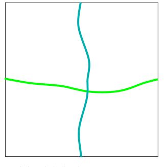
Figure 4.6: Strings localized at the intersection.

S-dual to quiver circle $\longrightarrow$

Quiver circle direction $\longrightarrow$

$b,\psi_{b}$

S-dual
                                                                                         to $b,\psi_{b}$

Note that the S-dual’s to the fundamental degrees of freedom at the intersection are strings wrapping the $S^{1}$ of the quiver diagram. Thus it is tempting to speculate that they can built from gauge invariant products of fundamental spoke degrees of freedom which wrap the quiver. An example of such an operator is ${\rm tr\,}\Lambda^{B}_{1,2}\Lambda^{\tilde{B}}_{2,3}\cdots\Lambda^{B}_{k-1,k}\Lambda^{\tilde{B}}_{k,1}$. On the other hand, one expects the S-dual operators to be solitons without an expression in terms of products of local operators, so this speculation is probably not quite correct.

String condensation and M5-branes on a holomorphic curve

When tensionless strings condense, the M5-M5 intersection is resolved to the holomorphic curve $xy=c$. This can be seen very explicitly from compactification on a torus. In this case the low energy theory is that of the D3-D3 intersection in flat space. In Sec. 2.5.4 we showed that the Higgs branch of the corresponding $(4,4)$ dCFT can be interpreted as a resolution of the intersection to the holomorphic curve $xy=c$. The resolved intersection is also clearly captured by the $(4,0)$ dCFT. At the point in the moduli space for which extra dimensions are generated, the $(4,0)$ dCFT reduces to the $(4,4)$ dCFT at low energies. The potential is minimized by restricting to fields with values independent of the quiver index $j$ and satisfying equations equivalent to (2.106). The holomorphic curve $xy=c$ arises when the fields $B_{j}$ and $\tilde{B}_{j}$ get expectation values independent of $j$. These fields correspond to tensionless strings at the M5-M5 intersection.

Identifying R-symmetries and moduli

The M5-M5 intersection has ${\cal N}=2,d=4$ supersymmetry with $SU(2)\times U(1)$ R-symmetry. We would like to identify the corresponding charges in the $(4,0)$ defect conformal field theory.

For the $U(1)$ R-symmetry, the identification is as follows. This symmetry is manifest in both cases and corresponds to a simultaneous rotation of the $x$ and $y$ planes, which are transverse to one stack of parallel branes but not the orthogonal stack. In the $(4,0)$ dCFT, it is generated by $J_{23}-J_{45}$, and the associated charges can be readily obtained from Tab. 2.2. Note that the other linear combination, $J_{23}+J_{45}$, is not an R-symmetry, and acts trivially on the degrees of freedom localized at the intersection.

We will now argue that the $SU(2)_{L}$ R-symmetry of the $(4,0)$ dCFT should be identified with the $SU(2)$ R-symmetry of the ${\cal N}=2,d=4$ theory of the M5-brane intersection. This matching is non-trivial for the following reason. In order to generate the extra dimensions, it was necessary to consider a point on the Higgs branch where the $SU(2)_{L}$ doublets $\langle Y\rangle$ and $\langle Y^{\prime}\rangle$ are non-zero, so that $SU(2)_{L}$ is spontaneously broken. On the other hand the $SU(2)$ R-symmetry of the M5-M5 intersection is only broken when M5-branes are transversely separated. Nevertheless, we shall find evidence that the identification makes sense. This suggests that when the M5-branes are not separated, the $SU(2)_{L}$ symmetry of the $(4,0)$ dCFT description is unbroken as far as the non-trivial dynamics is concerned.

There are three directions transverse to both stacks of M5-branes, corresponding to the moduli $\vec{X}$ and $\vec{X}^{\prime}$, which form a triplet under the $SU(2)$ R-symmetry. This R-symmetry is spontaneously broken if either $\vec{X}$ or $\vec{X}^{\prime}$ is non-zero. However if all the eigenvalues of $\vec{X}$ and $\vec{X}^{\prime}$ are the same, then the symmetry breaking is due only to trivial center of mass dynamics. The string tension $T=|\vec{X}-\vec{X}^{\prime}|$ vanishes at this point.

In the $(4,0)$ dCFT, the point in moduli space described by (4.45) corresponds to a string tension $T=v\Delta$. If we act with $SU(2)_{L}$, we obtain another point in moduli space which also deconstructs the same configuration of intersecting M5-branes. The string tension can be written in an $SU(2)_{L}$ invariant way as the expectation value of $|Y^{\dagger}\vec{\sigma}Y-{Y^{\prime}}^{\dagger}\vec{\sigma}Y^{\prime}|$ where $\vec{\sigma}$ are Pauli matrices. We have dropped the $j,j+1$ subscript as we only consider the zero momentum modes in the (de)constructed directions. On the other hand the string tension is related to the moduli of the M5-M5 intersection by $T=|\vec{X}-\vec{X}^{\prime}|$. This motivates the proposal

$$\vec{X}-\vec{X}^{\prime}\sim Y^{\dagger}\vec{\sigma}Y-{Y^{\prime}}^{\dagger}\vec{\sigma}Y^{\prime}\,.$$ (4.50)

Under $SU(2)_{L}$, $Y^{\dagger}\vec{\sigma}Y-{Y^{\prime}}^{\dagger}\vec{\sigma}Y^{\prime}$ transforms as a triplet, while $\vec{X}-\vec{X}^{\prime}$ transforms as triplet under $SU(2)$. This suggests that one should identify the $SU(2)_{L}$ R-symmetry of the $(4,0)$ theory with the $SU(2)$ R-symmetry of the M5-M5 intersection.

Thus far we have neglected a degree of freedom in the moduli space which also contributes to the string tension. There are four degrees of freedom in either $Y$ and or $Y^{\prime}$, while only three are characterised by $Y^{\dagger}\vec{\sigma}Y$ or ${Y^{\prime}}^{\dagger}\vec{\sigma}Y^{\prime}$. Note that $Y^{\dagger}\vec{\sigma}Y$ is invariant under $Y\rightarrow e^{i\theta}Y$, so the missing degree of freedom is an angle. The quantity $|Y^{\dagger}\vec{\sigma}Y-{Y^{\prime}}^{\dagger}\vec{\sigma}Y^{\prime}|=4vRe(\Delta)$ only gives the string tension for real $\Delta$. For complex $\Delta$ the string tension is easily seen to be $v|\Delta|$. The imaginary part of $\Delta$ corresponds to the additional angular degree of freedom. That the imaginary part is an angle is evident from the orbifold condition $(u,\bar{w})\sim\exp(2\pi i/k)(u,\bar{w})$ which for large $k$ gives $\Delta\sim\Delta+2\pi iv/k$. By viewing the quiver action as an action with only one extra discretized dimension (i.e. taking $R_{6}\rightarrow 0$ with fixed $R_{5}$), one discovers that the angular degree of freedom is a gauge connection in the compact discretized fifth direction. If the associated Wilson lines differ for the two intersecting branes, a mass term is generated for the degrees of freedom localized at the intersection. In terms of the six dimensional theories, this Wilson line may be interpreted as a Wilson surface corresponding to the holonomy of the mysterious non-abelian two-form on the torus.

4.5 Deconstruction of M-theory on $T^{3}\times A_{N-1}$

The deconstruction of extra dimensions is also possible in theories including gravity. Discrete gravitational extra dimensions were studied in [108, 109, 110, 111, 112]. The basic idea is to consider $d+1$-dimensional Einstein gravity as the low-energy effective theory of a $d$-dimensional gravitational theory with a discrete theory space. The continuum physics of the $d+1$-dimensional gravitational theory can be reproduced correctly at energies parametrically higher than the compactification scale. However, a peculiar UV/IR connection was found forbidding the deconstruction all the way up to the $d+1$-dimensional Planck scale.

As a special gravitational theory, it would be very interesting to deconstruct M-theory itself. In [113] it was proposed to deconstruct M-theory on an $A_{N-1}$ singularity from a particular $(1,0)$ little string theory (LST). This LST is defined as the decoupling limit of $N$ NS5-branes at an orbifold singularity of the type $\mathbb{C}^{2}/\mathbb{Z}_{k}$. A seventh dimension arises on the Higgs branch of this theory. In a continuum ($k\rightarrow\infty$) limit one expects to obtain a seven-dimensional gauge theory together with its UV completion. Exploiting string dualities for $k\rightarrow\infty$, it was shown [113] that the stack of NS5-branes maps to M-theory on $A_{N-1}$, which is a UV completion of the seven-dimensional gauge theory.

A direct deconstruction seems to be impossible due to the obstructions to finding a (conventional) Lagrangian description for LST. Alternatively, one could first deconstruct the NS5-brane theory out of the D3-brane theory at $\mathbb{C}^{3}/\mathbb{Z}_{N_{5}}\times\mathbb{Z}_{N_{6}}$ [113]. One obtains a lattice action for LST which could in principle be orbifolded again by projecting out degrees of freedom which are not invariant under the (second) orbifold $\mathbb{C}^{2}/\mathbb{Z}_{k}$. Here one faces the problem that it is difficult, if not impossible, to find an $SU(2)$ R-symmetry inside the lattice action into which the $\mathbb{Z}_{k}$ orbifold action can be embedded. Note that the $SO(4)$ R-symmetry of the NS5-brane theory is only recovered in the continuum limit. It is therefore not obvious how to further discretize the latticized LST action.

In the following we apply the deconstruction method to M-theory following a slightly different approach. We deconstruct M-theory directly from a four-dimensional non-supersymmetric quiver gauge theory with gauge group $SU(N)^{N_{4}N_{6}N_{8}}$ and $N_{4,6,8}$ three positive integers. The corresponding orbifold realization is given by a stack of D3-branes in type IIB string theory placed at the origin of $\mathbb{C}^{3}/\Gamma$, where the orbifold group $\Gamma$ is the product of three cyclic groups $\mathbb{Z}_{N_{4}}\times\mathbb{Z}_{N_{6}}\times\mathbb{Z}_{N_{8}}$. These groups generate three circular orbits in the directions 468. The quiver diagram is a three-dimensional body-centred cubic lattice. At a certain point in the moduli space, each of the $\mathbb{Z}_{N}$ factors generates a circular discretized extra dimension. In an appropriate $N_{4,6,8}\rightarrow\infty$ limit, the extra dimensions become continuous, such that the theory appears to be seven-dimensional on the Higgs branch. There is however a peculiarity in this deconstruction which suggests that the strongly coupled Higgs branch theory is actually an eleven-dimensional gravitational theory: The deconstructed seven-dimensional gauge theory has a UV completion in terms of M-theory on $A_{N-1}$. In the brane realization of the present deconstruction, M-theory on $A_{N-1}$ arises naturally in the continuum limit.

The Higgs branch of the quiver theory corresponds to the decoupling limit of D3-branes a finite distance away from the orbifold singularity. In the limit which we will consider the D3-branes probe an approximate $\mathbb{R}^{3}\times T^{3}$ geometry. The generation of three extra dimensions along the Higgs branch corresponds to T-dualizing along the three circular dimensions of the three-torus $T^{3}$, giving D6-branes wrapped on $T^{3}$. The seven-dimensional gauge theory living on the D6-branes does not decouple from the bulk degrees of freedom, such that the deconstructed theory is not just a seven-dimensional gauge theory. Due to a strong type IIA string coupling $g_{s}$ a better description is obtained by lifting to M-theory. The D6-branes in type IIA string theory lift to M-theory on an $A_{N-1}$ singularity. This suggests the equivalence of M-theory on $A_{N-1}$ with the continuum limit of the present quiver theory.

4.5.1 D3-branes at $\mathbb{C}^{3}/\mathbb{Z}_{N_{4}}\times\mathbb{Z}_{N_{6}}\times\mathbb{Z}_{N_{8}}$: orbifold realization of a non-supersymmetric quiver theory

In this section we discuss the quiver theory, from which we deconstruct M-theory. The quiver theory is a four-dimensional non-supersymmetric field theory with gauge group $SU(N)^{N_{4}N_{6}N_{8}}$. This theory describes the decoupling limit of $NN_{4}N_{6}N_{8}$ D3-branes in type IIB string theory placed at a $\mathbb{C}^{3}/\Gamma$ orbifold singularity with $\Gamma\equiv\mathbb{Z}_{N_{4}}\times\mathbb{Z}_{N_{6}}\times\mathbb{Z}_{N_{8}}$.

The orbifold action on the complex coordinates $z_{i}=(h,v,n)$ parameterizing $\mathbb{C}^{3}$ is given by

$$h\rightarrow\xi_{4}^{\,2}h\,,\qquad v\rightarrow\xi_{6}^{\,2}v\,,\qquad n\rightarrow\xi_{8}^{\,2}n\,,$$ (4.51)

where the generators of the groups $\mathbb{Z}_{N_{a}}$ are defined by $\xi_{a}=\exp(2\pi i/N_{a})$, $a=4,6,8$. Each of the factors $\mathbb{Z}_{N_{a}}$ ($a=4,6,8$) acts on one of the three complex planes transverse to the stack of D3-branes. The orbifold action can be embedded into the subgroup $U(1)^{3}$ of the rotational group $SO(6)$.

The fields of the quiver theory descend from the ${\cal N}=4,d=4$ vector multiplet of the parent super Yang-Mills theory with gauge group $U(NN_{4}N_{6}N_{8})$. We project out degrees of freedom which are not invariant under the orbifold group. The action of the product orbifold on the gauge field $A_{\mu}$, the three scalars $\phi^{i}=(h,v,n)$, and the four spinors $\psi^{i}=(\psi^{h},\psi^{v},\psi^{n},\lambda)$ is given by

$$A_{\mu} \rightarrow g(\xi)A_{\mu}g(\xi)^{-1}\,,$$ (4.52)

$$\phi^{i} \rightarrow\xi^{b^{(4)}_{i}}_{4}\xi^{b^{(6)}_{i}}_{6}\xi^{b^{(8)}_{i}}_{8}g(\xi)\phi^{i}g(\xi)^{-1}\,,$$ (4.53)

$$\psi^{i} \rightarrow\xi^{a^{(4)}_{i}}_{4}\xi^{a^{(6)}_{i}}_{6}\xi^{a^{(8)}_{i}}_{8}g(\xi)\psi^{i}g(\xi)^{-1}\,,$$ (4.54)

where $g(\xi)=g(\xi_{4})\otimes g(\xi_{6})\otimes g(\xi_{8})$ is the regular representation of the generator $\xi=\xi_{4}\xi_{6}\xi_{8}$ of $\Gamma$. These transformation rules extend the invariance conditions given by Eqns. (4.2)-(4.5). For the vectors $a_{i}$ and $b_{i}$ we choose:

$$\mathbb{Z}_{N_{4}}:\quad a^{(4)}_{i} =(-1,1,1,-1)\,,\quad b^{(4)}_{i}=(2,0,0)\,,$$ (4.55)

$$\mathbb{Z}_{N_{6}}:\quad a^{(6)}_{i} =(1,-1,1,-1)\,,\quad b^{(6)}_{i}=(0,2,0)\,,$$ (4.56)

$$\mathbb{Z}_{N_{8}}:\quad a^{(8)}_{i} =(1,1,-1,-1)\,,\quad b^{(8)}_{i}=(0,0,2)\,.$$ (4.57)

Each of the three pairs of vectors ($a_{i},b_{i}$) gives rise to an orbifold $\mathbb{C}/\mathbb{Z}_{N}$ of the type given by Eq. (4.7). Together they define the non-supersymmetric orbifold $\mathbb{C}^{3}/\mathbb{Z}_{N_{4}}\times\mathbb{Z}_{N_{6}}\times\mathbb{Z}_{N_{8}}$. The vectors $b_{i}$ determine the action (4.51) on the coordinates $z_{i}=(h,v,n)$ via

$$z_{i}\rightarrow\xi^{b^{(4)}_{i}}_{4}\xi^{b^{(6)}_{i}}_{6}\xi^{b^{(8)}_{i}}_{8}z_{i}\,.$$ (4.58)

The vectors $a_{i}$ give the corresponding action on the four fermions. The invariant fermions $\psi^{m}_{i,j,k}$ transform under the gauge group

$$SU(N)^{N_{4}N_{6}N_{8}}$$ (4.59)

as $({\rm N}_{i,j,k},\overline{\rm N}_{i\pm a^{(4)}_{m},j\pm a^{(6)}_{m},k\pm a^{(8)}_{m}})$, where N_i,j,k ($\overline{\rm N}_{i^{\prime},j^{\prime},k^{\prime}}$) denotes the (anti-)fundamental representation of the gauge group $SU(N)_{i,j,k}$ ($SU(N)_{i^{\prime},j^{\prime},k^{\prime}}$). The invariant scalars $\phi^{m}_{i,j,k}$ transform as $({\rm N}_{i,j,k},\overline{\rm N}_{i\pm b^{(4)}_{m},j\pm b^{(6)}_{m},k\pm b^{(8)}_{m}})$. We summarize the field content of our quiver theory in the Tab. 4.1.

field	representation	field	representation
$h_{i,j,k}$	$({\rm N}_{i,j,k},\overline{\rm N}_{i+2,j,k})$	$\psi^{h}_{i,j,k}$	$({\rm N}_{i,j,k},\overline{\rm N}_{i+1,j-1,k-1})$
$v_{i,j,k}$	$({\rm N}_{i,j,k},\overline{\rm N}_{i,j+2,k})$	$\psi^{v}_{i,j,k}$	$({\rm N}_{i,j,k},\overline{\rm N}_{i-1,j+1,k-1})$
$n_{i,j,k}$	$({\rm N}_{i,j,k},\overline{\rm N}_{i,j,k+2})$	$\psi^{n}_{i,j,k}$	$({\rm N}_{i,j,k},\overline{\rm N}_{i-1,j-1,k+1})$
$A^{\mu}_{i,j,k}$	adjoint	$\lambda_{i,j,k}$	$({\rm N}_{i,j,k},\overline{\rm N}_{i+1,j+1,k+1})$

Table 4.1: Fields in the quiver theory and their transformation behaviour under the gauge group $SU(N)^{N_{4}N_{6}N_{8}}$.

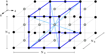
Figure 4.7: Theory space for the $\mathbb{Z}_{N_{4}}\times\mathbb{Z}_{N_{6}}\times\mathbb{Z}_{N_{8}}$ quiver theory. Dark and light (blue) lines in the basic cell represent bosonic and fermionic bifundamentals. Dotted lines are not physical and are just to guide the eye.

The theory space is a three-dimensional lattice with $N_{4}N_{6}N_{8}$ sites which discretizes a three-dimensional torus $T^{3}$ as shown in Fig. 4.7. Each site represents one of the gauge groups $SU(N)_{i,j,k}$ and its associated gauge boson $A^{\mu}_{i,j,k}$. Link fields start at a site $i,j,k$, where they transform in the fundamental representation ${\rm N}_{i,j,k}$, and end at a site $i^{\prime},j^{\prime},k^{\prime}$, where they transform in the anti-fundamental representation $\overline{\rm N}_{i^{\prime},j^{\prime},k^{\prime}}$. Fig. 4.7 shows the unit cell of the lattice spanned by the link fields. The bosonic bifundamentals $h_{i,j,k}$, $v_{i,j,k}$, $n_{i,j,k}$ (dark lines) form the edges of the unit cell, while the fermionic bifundamentals $\psi^{h}_{i,j,k},\psi^{v}_{i,j,k},\psi^{n}_{i,j,k},\lambda_{i,j,k}$ (light lines) connect the corners with the centre of the cell. Translating the unit cell in the lattice we obtain a body-centred cubic lattice which is invariant under the 48 element octahedral symmetry group $O_{h}$. Such bcc lattices were also studied in the context of four-dimensional ${\cal N}=4$ super Yang-Mills theory on a three-dimensional lattice [107].

Let us now construct the Lagrangian for our orbifold model which consists of three parts,

$${\cal L}={\cal L}_{\rm kin}+{\cal L}_{\rm Yuk}+{\cal L}_{\rm quartic}\,.$$ (4.60)

This Lagrangian follows from four-dimensional ${\cal N}=4$ super Yang-Mills theory with gauge group $U(NN_{4}N_{6}N_{8})$ upon projecting out degrees of freedom which are not invariant under the orbifold group. The kinetic terms have the form

$${\cal L}_{\rm kin}\supset\frac{1}{2}{\rm Tr}(D_{\mu}\varphi_{i^{\prime},j^{\prime},k^{\prime}})^{\dagger}D^{\mu}\varphi_{i,j,k}\,,$$ (4.61)

where the field $\varphi_{i,j,k}$ is one of the seven bifundamentals transforming in the $({\rm N}_{i,j,k},\overline{\rm N}_{i^{\prime},j^{\prime},k^{\prime}})$ as listed in Tab. 4.1. The covariant derivative of $\varphi_{i,j,k}$ is defined by

$$D_{\mu}\varphi_{i,j,k}=\partial_{\mu}\varphi_{i,j,k}-igA^{i,j,k}_{\mu}\varphi_{i,j,k}+ig\varphi_{i,j,k}A^{i^{\prime},j^{\prime},k^{\prime}}_{\mu}\,.$$ (4.62)

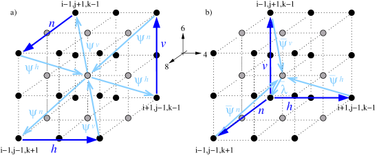
Figure 4.8: Oriented link fields in the basic cell. The site in the centre of the cell has labels $i,j,k$. The triangles represent possible Yukawa couplings in the quiver action.

We now consider the Yukawa and quartic scalar interactions ${\cal L}_{\rm Yuk}$ and ${\cal L}_{\rm quartic}$. Fig. 4.8 shows six of twelve possible triangles inside the basic cell. These triangles consist of two fermionic and one bosonic arrow and correspond to Yukawa couplings in the quiver theory. Each of the twelve triangles leads to a Yukawa term in the action.

For the Lagrangian ${\cal L}_{\rm Yuk}$ we thus find

$${\cal L}_{\rm Yuk}={\cal L}^{1}_{\rm Yuk}+{\cal L}^{2}_{\rm Yuk}\,,$$ (4.63)

with

$$\!\!\!\!\!\!{\cal L}^{1}_{\rm Yuk} =i\sqrt{2}g{\,\rm Tr}(\psi^{v}_{i,j,k}n_{i-1,j+1,k-1}\psi^{h}_{i-1,j+1,k+1}-\psi^{n}_{i,j,k}v_{i-1,j-1,k+1}\psi^{h}_{i-1,j+1,k+1}$$

$$\,+\psi^{n}_{i,j,k}h_{i-1,j-1,k+1}\psi^{v}_{i+1,j-1,k+1}-\psi^{h}_{i,j,k}n_{i+1,j-1,k-1}\psi^{v}_{i+1,j-1,k+1}$$ (4.64)

$$\,+\psi^{h}_{i,j,k}v_{i+1,j-1,k-1}\psi^{v}_{i+1,j+1,k-1}-\psi^{v}_{i,j,k}h_{i-1,j+1,k-1}\psi^{n}_{i+1,j+1,k-1}+c.c.)$$

and

$$\!\!\!\!\!\!{\cal L}^{2}_{\rm Yuk} =i\sqrt{2}g{\,\rm Tr}(\bar{\lambda}_{i,j,k}h_{i-1,j-1,k-1}\bar{\psi}^{h}_{i+1,j-1,k-1}-\bar{\psi}^{h}_{i,j,k}h_{i-1,j+1,k+1}\bar{\lambda}_{i+1,j+1,k+1}$$

$$+\bar{\lambda}_{i,j,k}v_{i-1,j-1,k-1}\bar{\psi}^{v}_{i-1,j+1,k-1}-\bar{\psi}^{v}_{i,j,k}v_{i+1,j-1,k+1}\bar{\lambda}_{i+1,j+1,k+1}$$ (4.65)

$$+\bar{\lambda}_{i,j,k}n_{i-1,j-1,k-1}\bar{\psi}^{n}_{i-1,j-1,k+1}-\bar{\psi}^{n}_{i,j,k}n_{i+1,j+1,k-1}\bar{\lambda}_{i+1,j+1,k+1}+c.c.)\,,$$

where summation over $i,j,k$ is understood. The terms with a positive sign in ${\cal L}^{1}_{\rm Yuk}$(${\cal L}^{2}_{\rm Yuk}$) correspond to the triangles in Fig. 4.8a(b) (those with negative sign are not shown). The Yukawa couplings in ${\cal L}^{1}_{\rm Yuk}$ descend from the ${\cal N}=4$ superpotential $[H,V]N$, while those in ${\cal L}^{2}_{\rm Yuk}$ come from the Kähler potential.

Quite analogously, squares in the quiver diagram represent quartic scalar terms which are given by

$$\!\!\!\!\!\!{\cal L}_{\rm quartic} =g^{2}{\,\rm Tr}(n_{i,j,k}h_{i,j,k+2}\bar{n}_{i+2,j,k+2}\bar{h}_{i+2,j,k}-h_{i,j,k}n_{i+2,j,k}\bar{h}_{i+2,j,k+2}\bar{n}_{i,j,k+2}$$

$$+h_{i,j,k}v_{i+2,j,k}\bar{h}_{i+2,j+2,k}\bar{v}_{i,j+2,k}-v_{i,j,k}h_{i,j+2,k}\bar{v}_{i+2,j+2,k}\bar{h}_{i+2,j,k}$$ (4.66)

$$+v_{i,j,k}n_{i,j+2,k}\bar{v}_{i,j+2,k+2}\bar{n}_{i,j,k+2}-n_{i,j,k}v_{i,j,k+2}\bar{n}_{i,j+2,k+2}\bar{v}_{i,j+2,k})\,.$$

This model belongs to the class of conformal non-supersymmetric orbifold models studied in [166, 167]. In these models it is assumed that the orbifold group $\Gamma\subset SU(4)$ acts solely on the transverse space $\mathbb{C}^{3}$ of $M$ parallel D3-branes. Kachru and Silverstein [168] noticed that the orbifold group acts only on the $S^{5}$ factor of the near horizon geometry $AdS_{5}\times S^{5}$. In the AdS/CFT correspondence the isometry group of the $AdS_{5}$ space is identified with the conformal group of the field theory on its boundary. This implies classical conformal invariance of the world-volume theory on the D3-branes. In [166] it was shown that if $M$ is finite and the regular representation of $\Gamma$ is chosen, the one-loop beta functions for the gauge couplings vanish in these theories. In the large $M$ limit one can even prove the vanishing of the beta functions to all orders in perturbation theory [167]. This holds for the present quiver theory which we consider in the limit $N_{4,6,8}\rightarrow\infty$ such that $M=N\,N_{4}N_{6}N_{8}\rightarrow\infty$. Our non-supersymmetric quiver theory has therefore quantum conformal invariance. As discussed in detail in [113] conformal invariance guarantees that the quiver theory remains in the Higgs phase even at strong coupling.

A related question to that of conformal invariance is the stability of the moduli space. Since the theory is not supersymmetric the potential for the scalars is not necessarily protected against quantum corrections. This would change the moduli space of the classical theory. However, as shown in [167] all Feynman diagrams in the quiver theory are the same as in the ${\cal N}=4$ parent $U(M)$ gauge theory up to possible $\frac{1}{M}$ corrections. In the large $M$ limit these corrections are suppressed and the potential remains unchanged. Although this points to a stable moduli space, we might still have troubles with divergencies coming from the twisted closed string sector.

The question of stability of our model is highly non-trivial. In contrast to supersymmetric orbifold models there are closed string tachyons in the twisted sector of non-supersymmetric orbifolds of the type $\mathbb{C}/\mathbb{Z}_{N}$. The tachyon condensation leads to the decay of the orbifold as studied in [169]. The initial effect of the tachyons is to smooth out the orbifold singularity. An RG flow is initiated by the tachyon and the orbifold decays to flat space. If the initial state has been appropriately fine-tuned, the orbifold decay can take place in a series of transitions $\mathbb{C}/\mathbb{Z}_{N}\rightarrow\mathbb{C}/\mathbb{Z}_{N-2}$. For finite $N$ the orbifold becomes flat in a finite time. However, in the limit $N\rightarrow\infty$ the orbifold does not decay in a finite amount of time, since the orbifold goes through only finitely many transitions $\mathbb{C}/\mathbb{Z}_{N}\rightarrow\mathbb{C}/\mathbb{Z}_{N-2}$. The orbifold may however decay faster, e.g. via transitions $\mathbb{C}/\mathbb{Z}_{N}\rightarrow\mathbb{C}/\mathbb{Z}_{N-M}$ ($M>2$). If the quotient $M/N$ vanishes in the large $N$ limit the orbifold remains stable. In other words, the question is whether the flattening of spacetime induced by the tachyon condensation outweighs the extreme curvature at the singularity. We believe it does not and presume that our model is stable in the large $N_{4,6,8}$ limit. However, this issue deserves some further investigation.

Another essential feature in the deconstruction of M-theory is S-duality of the orbifold model. In [166] it was argued that in a conformal (non-supersymmetric) quiver theory the complex moduli $\tau_{i}$ are inherited from the coupling $\tau_{\rm par}$ of the ${\cal N}=4$ parent theory (recall $\tau_{i}=\tau_{\rm par}/|\Gamma|$). In the present quiver theory the $N_{4}N_{6}N_{8}$ gauge couplings $\tau_{i,j,k}$ associated with the gauge groups $SU(N)_{i,j,k}$ are all the same and related to $\tau_{\rm par}$ by

$$\tau\equiv\tau_{i,j,k}=\frac{\tau_{\rm par}}{N_{4}N_{6}N_{8}}\,.$$ (4.70)

The strong-weak duality $g_{\rm par}\rightarrow 1/g_{\rm par}$ thus amounts to an $SL(2,\mathbb{Z})$ S-duality $g\rightarrow N_{4}N_{6}N_{8}/g$ in the quiver theory.

4.5.2 Generation of three compact extra dimensions in the low-energy effective field theory

We now show by studying the mass spectrum of the gauge bosons that the quiver theory generates three circular extra dimensions at low energies. On the Higgs branch of the theory the scalar bifundamentals have expectation values,

$$\langle h_{i,j,k}\rangle=v_{4}\,,\qquad\langle v_{i,j,k}\rangle=v_{6}\,,\qquad\langle n_{i,j,k}\rangle=v_{8}\,,$$ (4.71)

independent of $i,j,k$. These condensates break the gauge group $SU(N)^{N_{4}N_{6}N_{8}}$ down to the diagonal subgroup $SU(N)$. Upon substituting the vevs $v_{4},v_{6},v_{8}$, the scalar kinetic terms inside ${\cal L}_{\rm kin}$ give rise to mass terms for the gauge bosons,

$${\rm Tr}|D^{\mu}h_{i,j,k}|^{2} =g^{2}v^{2}_{4}(A_{\mu}^{i,j,k}-A_{\mu}^{i+2,j,k})^{2}\equiv A_{\mu}^{i,j,k}({\cal M}_{4})^{2}_{ii^{\prime}}\delta_{jj^{\prime}}\delta_{kk^{\prime}}A^{\mu}_{i^{\prime},j^{\prime},k^{\prime}}$$

$${\rm Tr}|D^{\mu}v_{i,j,k}|^{2} =g^{2}v^{2}_{6}(A_{\mu}^{i,j,k}-A_{\mu}^{i,j+2,k})^{2}\equiv A_{\mu}^{i,j,k}\delta_{ii^{\prime}}({\cal M}_{6})^{2}_{jj^{\prime}}\delta_{kk^{\prime}}A^{\mu}_{i^{\prime},j^{\prime},k^{\prime}}$$ (4.72)

$${\rm Tr}|D^{\mu}n_{i,j,k}|^{2} =g^{2}v^{2}_{8}(A_{\mu}^{i,j,k}-A_{\mu}^{i,j,k+2})^{2}\equiv A_{\mu}^{i,j,k}\delta_{ii^{\prime}}\delta_{jj^{\prime}}({\cal M}_{8})^{2}_{kk^{\prime}}A^{\mu}_{i^{\prime},j^{\prime},k^{\prime}}\,.$$

The matrices ${\cal M}_{4,6,8}$ have entries $2$ on the diagonal and $-1$ on the second off-diagonal. As in [138] diagonalization of the mass matrices ${\cal M}_{4,6,8}$ yields the mass eigenvalues

$$m^{k}_{4,6,8}=2gv_{4,6,8}\sin\frac{2\pi k}{N_{4,6,8}}\approx 2gv_{4,6,8}\frac{2\pi k}{N_{4,6,8}}\quad{\rm for\,\,}k\ll N_{4,6,8}\,.$$ (4.73)

For small enough $k$, this approximates the Kaluza-Klein spectrum of a seven-dimensional gauge boson compactified on a three-torus $T^{3}$ with radii $R_{4,6,8}$. The radii $R_{4,6,8}$ are fixed by the mass scales of the lightest KK modes ($k=1$) which are given by

$$m_{4,6,8}=\frac{1}{R_{4,6,8}}\,,$$ (4.74)

with

$$2\pi R_{4}=N_{4}a_{4}=\frac{N_{4}}{2gv_{4}}\,,\quad 2\pi R_{6}=N_{6}a_{6}=\frac{N_{6}}{2gv_{6}}\,,\quad 2\pi R_{8}=N_{8}a_{8}=\frac{N_{8}}{2gv_{8}}\,$$ (4.75)

and $a_{4,6,8}$ the lattice spacings. In principle, this KK spectrum is not protected and could receive quantum corrections at strong coupling. In a similar context [113] it was argued that such quantum corrections are proportional to $\frac{1}{N_{4,6,8}}$ and vanish in the large $N_{4,6,8}$ limit. Provided this is true, we explicitly deconstruct three compact extra dimensions with radii $R_{4,6,8}$.

The Higgs mechanism does induce masses both for the gauge bosons as well as for the bifundamental fermions and scalars. For instance, substituting vevs for the scalars inside the Lagrangian ${\cal L}_{\rm Yuk}$ leads to fermionic mass terms. Such mass terms could in principle lead to a different mass spectrum due to the non-supersymmetric nature of our model. Following [22] one can however verify that the fermionic mass spectrum is identical to the gauge boson spectrum. Both the bosonic as well as the fermionic Kaluza-Klein spectra generate the same extra dimensions.

4.5.3 M2-branes on the Higgs branch

By studying the orbifold geometry we show in the next section that the Higgs branch theory is equivalent to M-theory on an $A_{N-1}$ singular geometry. We have seen that the Higgs branch theory contains seven-dimensional super Yang-Mills theory with gauge group $SU(N)$. In M-theory on $A_{N-1}$ the seven-dimensional $SU(N)$ gauge symmetry arises from M2-branes wrapping collapsed two-cycles at the singularity, see e.g. [170]. In other words, the deconstructed 7d super Yang-Mills theory is part of M-theory on $A_{N-1}$. However, M-theory contains more than just the 7d gauge theory. We have to verify also the existence of M2- or M5-branes inside the quiver theory.

The states corresponding to M2-branes can be seen in the dyonic spectrum of the quiver gauge theory. The dyonic mass spectrum follows from that of the gauge bosons by S-duality. Substituting

$$g\rightarrow\frac{N_{4}N_{6}N_{8}}{g}\,$$ (4.76)

into Eq. (4.74), we find for the lowest dyonic states the masses

$$M_{4}=8\pi^{3}R_{6}R_{8}/g^{2}_{7}\,,\qquad M_{6}=8\pi^{3}R_{8}R_{4}/g^{2}_{7}\,,\qquad M_{8}=8\pi^{3}R_{4}R_{6}/g^{2}_{7}\,,$$ (4.77)

where the seven-dimensional coupling constant is $g_{7}^{2}=a_{4}a_{6}a_{8}g^{2}$. These masses are identical to those of two-branes wrapping around two-tori $T^{2}$ inside the $T^{3}$. We can read off the tension of the two-branes, $T_{2}=1/(2\pi)^{2}g_{7}^{2}$, which is identical to the tension of M2-branes, $T_{\rm M2}=1/(2\pi)^{2}l_{p}^{3}$. This gives field-theoretical evidence that we really deconstruct M-theory.

4.5.4 Summary of the field theory results

Let us summarize the properties of the $SU(N)^{N_{4}N_{6}N_{8}}$ quiver theory. We have seen that three extra dimensions with fixed radii $R_{4,6,8}$ are generated along the Higgs branch defined by Eq. (4.71). For finite lattice spacings $a_{4,6,8}$ our four-dimensional quiver theory describes a seven-dimensional theory with gauge coupling $g_{7}^{2}$ discretized on a three-dimensional toroidal lattice. Seven-dimensional super Yang-Mills theory breaks down at a certain cut-off $\Lambda_{\rm 7d}$ above which it requires a UV completion. The cut-off of the deconstructed theory is given by the mass of the highest KK mode, $\Lambda=a^{-1}$ ($a=\max[a_{4},a_{6},a_{8}]$). In the continuum limit $a_{4,6,8}\rightarrow 0$, which requires $g\rightarrow\infty$ while keeping the radii $R_{4,6,8}$ and the seven-dimensional gauge coupling $g_{7}^{2}$ fixed, $\Lambda$ becomes very large, $\Lambda\gg\Lambda_{\rm 7d}$. In the large $N_{4,6,8}$ limit we therefore expect to deconstruct not only 7d super Yang-Mills theory but also its UV completion. This is shown schematically in Fig. 4.9. We show in the next section that the UV completion is M-theory on $A_{N-1}$ with Planck length $l_{p}^{3}=g_{7}^{2}$.

Figure 4.9: Various cut-offs in the deconstruction of M-theory.

M-theory on this geometry consists of two parts: The seven-dimensional gauge theory living on the singularity of the $A_{N-1}$ space couples to the eleven-dimensional bulk degrees of freedom of M-theory. In the gauge boson spectrum, we can therefore see only three of the seven string-theoretically predicted extra dimensions. It is not quite clear how the four dimensions of the $A_{N-1}$ space are generated. However, we have found a spectrum of massive dyons showing the presence of M2-branes in the deconstructed theory. This supports our conjecture that the deconstructed theory is M-theory on $A_{N-1}$.

4.5.5 String-theoretical motivation for the equivalence

We now motivate the conjecture of the last section by a string-theoretical analysis of the orbifold geometry. The discussion will be similar to that in Sec. 4.3.2. We show that supersymmetry with 16 supercharges is restored on the Higgs branch of our model, where the theory becomes M-theory on a $T^{3}\times A_{N-1}$ geometry. To this end, we consider the behaviour of the stack of D3-branes on the Higgs branch.

For this purpose, let us study the geometry of the orbifold in the vicinity of the D3-branes which are located a distance $d$ away from the orbifold singularity. The product orbifold $\mathbb{C}^{3}/\mathbb{Z}_{N_{4}}\times\mathbb{Z}_{N_{6}}\times\mathbb{Z}_{N_{8}}$ can be parameterized by the complex coordinates ($i=1,2,3$) [124]

$$z_{i}=r_{i}\exp\left(i\frac{b^{(4)}_{i}}{N_{4}}\theta_{1}+i\frac{b^{(6)}_{i}}{N_{6}}\theta_{2}+i\frac{b^{(8)}_{i}}{N_{8}}\theta_{3}\right)\,.$$ (4.78)

For orthogonal vectors $b^{(4)}_{i},b^{(6)}_{i},b^{(8)}_{i}$, the orbifold metric $ds^{2}=dz_{i}d\bar{z}_{i}$ acquires the form

$$ds^{2}=d\vec{r}^{\,2}+\frac{({\vec{r}}\cdot{\vec{b}}^{(4)})^{2}}{N_{4}^{2}}d\theta_{1}^{2}+\frac{({\vec{r}}\cdot{\vec{b}}^{(6)})^{2}}{N_{6}^{2}}d\theta_{2}^{2}+\frac{({\vec{r}}\cdot{\vec{b}}^{(8)})^{2}}{N_{8}^{2}}d\theta_{3}^{2}\,,$$ (4.79)

where $\vec{r}=(r_{1},r_{2},r_{3})$, $\vec{b}^{(4)}=(b^{(4)}_{1},b^{(4)}_{2},b^{(4)}_{3})$, etc. The orbifold has the geometry of a three-torus fibration over $\mathbb{R}^{3}$: We recover three circles $S^{1}$ parameterized by $\theta_{1,2,3}\in[0,2\pi]$. For the particular choice of vectors $b_{i}$ as defined in Eqns. (4.55)-(4.57), the circles $S^{1}$ have radii $R_{S^{1}}={l_{s}^{2}}/{R_{4,6,8}}$ with the radii $R_{4,6,8}$ given by

$$R_{4}=\frac{N_{4}l_{s}^{2}}{2d_{4}}\,,\qquad R_{6}=\frac{N_{6}l_{s}^{2}}{2d_{6}}\,,\qquad R_{8}=\frac{N_{8}l_{s}^{2}}{2d_{8}}\,.$$ (4.80)

Here the D3-branes were assumed to be located at $\vec{r}=(d_{4},d_{6},d_{8})$. Comparison with the radii defined in (4.75) yields relations between the parameters of the quiver theory $g$, $v_{4,6,8}$, $N_{4,6,8}$ and the string theory parameters $l_{s}$, $g_{s}$, $d_{4,6,8}=|z_{1,2,3}|$, $N_{4,6,8}$:

$$\frac{d_{4}}{N_{4}l_{s}^{2}}=\frac{2\pi gv_{4}}{N_{4}}\,,\qquad\frac{d_{6}}{N_{6}l_{s}^{2}}=\frac{2\pi gv_{6}}{N_{6}}\,,\qquad\frac{d_{8}}{N_{8}l_{s}^{2}}=\frac{2\pi gv_{8}}{N_{8}}\,.$$ (4.81)

These relations show that giving vevs $v_{4},v_{6},v_{8}$ to the scalar bifundamentals $h,v,n$ corresponds to moving the D3-branes a distance $d=\sqrt{d_{4}^{2}+d_{6}^{2}+d_{8}^{2}}$ away from the singularity. The continuum limit $a_{4,6,8}\rightarrow 0$ keeping $R_{4,6,8}$ fixed is obtained if we take $l_{s}\rightarrow 0$, $N_{4,6,8}\rightarrow\infty$ with $g_{s}=g^{2}/N_{4}N_{6}N_{8}$ and $d_{4,6,8}/N_{4,6,8}l_{s}^{2}$ fixed.

The orbifold may be visualized as a product of three cones. In the large $N_{4,6,8}$ limit each of the cones locally degenerates into a cylinder $\mathbb{R}\times S^{1}$ similar as in Sec. 4.3.2, see also [113, 124]. The orbifold geometry in the vicinity of the D3-branes becomes approximately $\mathbb{R}^{3}\times T^{3}$ with $T^{3}$ a three-torus. Note that this induces a strong supersymmetry enhancement in the world-volume theory. The ${\cal N}=4$ super Yang-Mills parent theory preserves 16 supercharges. The orbifold projection reduces supersymmetry to ${\cal N}=0$. Now in the large $N_{4,6,8}$ limit, the D3-branes probe the geometry $\mathbb{R}^{3}\times T^{3}$, which in contrast to the orbifold, does not break supersymmetry. On the Higgs branch the supersymmetry of the quiver theory is therefore enhanced again to 16 supercharges.

In the large $N_{4,6,8}$ limit the radii of the three circles $S^{1}$ are sub-stringy, i.e. $R_{S^{1}}\ll l_{s}$ if $R_{4,6,8}\gg l_{s}$, and the appropriate description is obtained by T-dualizing along the three directions 468 of the three-torus. Details of the T-dualization are shown in Tab. 4.2.

duality	D3	$l_{s}\rightarrow 0$	$g_{s}$ fixed
T in $x^{4}$	D4	$l^{\prime}_{s}=l_{s}\rightarrow 0$	$g^{\prime}_{s}=g_{s}R_{4}/l_{s}\rightarrow\infty$
T in $x^{6}$	D5	$l^{\prime\prime}_{s}=l_{s}\rightarrow 0$	$g^{\prime\prime}_{s}=g_{s}R_{4}R_{6}/l^{2}_{s}\rightarrow\infty$
T in $x^{8}$	D6	$l^{\prime\prime\prime}_{s}=l_{s}\rightarrow 0$	$g^{\prime\prime\prime}_{s}=g_{s}R_{4}R_{6}R_{8}/l^{3}_{s}\rightarrow\infty$
M-theory	M-theory	$l^{3}_{p}=(l^{\prime\prime\prime}_{s})^{3}{g^{\prime\prime\prime}_{s}}$	$R_{11}=l^{\prime\prime\prime}_{s}{g^{\prime\prime\prime}_{s}}$
lift	on $A_{N-1}$	fixed

Table 4.2: T-dualization in $x^{4,6,8}$ and lift to M-theory.

We started from D3-branes in the decoupling limit $l_{s}\rightarrow 0$, $g_{s}$ fixed. These D3-branes T-dualize to D6-branes which wrap a three-torus $T^{3}$ with large radii $R_{4,6,8}$. Due to a large string coupling $g^{\prime\prime\prime}_{s}$, a more appropriate description is obtained by lifting the stack of $N$ D6-branes to a singular $A_{N-1}$ geometry in M-theory. The seven-dimensional gauge theory located on the $A_{N-1}$ singularity has gauge coupling $g_{7}^{2}=l_{p}^{3}=(l^{\prime\prime\prime}_{s})^{3}{g^{\prime\prime\prime}_{s}}=l^{2}_{s}R_{11}$. Since $R_{11}=g_{s}R_{4}R_{6}R_{8}/l^{2}_{s}\rightarrow\infty$ and $l_{s}\rightarrow 0$, we can hold both the gauge coupling $g_{7}$ and the eleven-dimensional Planck length $l_{p}$ fixed. The seven-dimensional gauge theory therefore does not decouple from the bulk gravity.

To conclude, string theory arguments suggest that our strongly coupled non-supersymmetric quiver theory on the Higgs branch describes M-theory on $T^{3}\times A_{N-1}$ in a large $N_{4,6,8}$ limit. Since M-theory reduces to eleven-dimensional supergravity at low-energies, we have deconstructed a gravitational theory!

5 Summary and conclusion

In this chapter we summarize the results found in Ch. 2–4 and give an outlook on possible future developments.

5.1 Results on dCFTs and their holographic duals

In Ch. 2 we discussed extensively the D3-D$p$ brane intersection as well as its dual probe-supergravity description. We have also presented the action and some of the elementary properties of a defect conformal field theory describing intersecting D3-branes, including some aspects of the AdS/CFT dictionary. There remain many interesting open questions, of which we enumerate a few below.

The defect conformal field theory corresponding to the D3-D3 intersection requires further field-theoretic analysis. One of the stranger features of this theory is that it contains massless two-dimensional scalars with (presumably) exactly marginal gauge, Yukawa, and scalar potential couplings. It is not at all obvious that one can construct a Hilbert space corresponding to operators with power law correlation functions, due to the logarithmic correlators of the two-dimensional scalars. It would be very interesting if one could show this to all orders in perturbation theory.

As a precursor to including gravity into the holographic map, it would be interesting to study the energy-momentum tensor of the defect conformal field theory in detail. We did not find any evidence of an enhancement of the two-dimensional $SO(2,2)$ global conformal symmetry to a full infinite-dimensional conformal symmetry on the two-dimensional defect. A study of the energy-momentum tensor would allow us to address this question conclusively at least from the field-theoretic side. For example, if an enhancement did indeed occur it should manifest itself in the form of a two-dimensional energy-momentum tensor which is holomorphically conserved.

Another question concerns the light-cone open string vacuum for D3-branes in the Penrose limit of the probe-supergravity background which we have considered. The operator proposed in [60] to correspond to the open string light-cone vacuum is not really a chiral primary and gives negative light-cone energy. This operator is precisely the one given in (2.97), and contains the dimensionless scalars which parameterize the Higgs branch. One might instead propose the operator ${\cal C}^{\mu l}$, with $P_{-}=\Delta-l=0$ as the dual of the light-cone vacuum, however this is only $1/4$ BPS and is in a non-trivial representation of the unbroken $SU(2)_{L}\times SU(2)_{R}$ R-symmetry. Presumably the subtleties regarding the light-cone vacuum are related to the quantum spreading over holomorphic embeddings $wy=c$ corresponding to the classical Higgs branch of the defect CFT. While the origin of this spreading is clear from the point of view of the dual defect CFT, and from the difficulties in finding localized supergravity solutions for intersecting D3-branes [68, 70, 69], they are not so clear from the point of view of a probe D3-brane embedded in the plane-wave or $AdS$ backgrounds.

Although there is presumably no fully localized supergravity solution for intersecting D3-branes, it would be surprising if there is no closed string description, in which both stacks of D3-branes are replaced by geometry. The problem of finding a closed string description of the theory raises a closely related question of how new degrees of freedom appear when $1/N$ (or $g_{s}$) corrections are taken into account in probe-supergravity background which we have considered. In constructing the holographic dual of the defect CFT, we have fixed the number $N^{\prime}$ of D3-branes in one stack, while taking the number $N$ of D3-branes in the orthogonal stack to infinity. In this limit, the degrees of freedom on one four-dimensional part of the world volume of the defect become free. The remaining coupled degrees of freedom live on a four-dimensional world volume and a two-dimensional defect, which are the boundaries of $AdS_{5}$ and the embedded $AdS_{3}$ respectively. Because the defect degrees of freedom are in the fundamental representation, the genus expansion of Feynman diagrams resembles an open string world-sheet expansion. When $1/N$ corrections are taken into account, the decoupled degrees of freedom must somehow reappear. The defect degrees of freedom become bi-fundamental fields with respect to a $SU(N)\times SU(N^{\prime})$ gauge group. The genus expansion for Feynman diagrams of the theory can now be viewed as a closed string world-sheet expansion, where a new branch of the target space has opened up.

Finally, the string theory realization of the defect CFT leads one to expect that it exhibits S-duality. It would be very interesting to find some field theoretic evidence for this. In particular one would need to find the S-duals of the fundamental degrees of freedom localized at the intersection.

5.2 Results on AdS/CFT with flavour

In Ch. 3 we have studied two non-supersymmetric gravity backgrounds with embedded D7-brane probes, corresponding to Yang-Mills theories with confined fundamental matter. The AdS Schwarzschild black-hole background which in the presence of the probe describes an ${\cal N}=2$ Yang-Mills theory at finite temperature, exhibits interesting behaviour such as a bilinear quark condensate and a geometric transition which corresponds to a first order transition in the gauge theory. The D7-brane embedding into the Constable-Myers background is more QCD-like, showing a chiral condensate at small quark mass as well as the accompanying pion (or large $N$ $\eta^{\prime}$).

In the Constable-Myers background with a D7-brane, there is a spontaneously broken $U(1)$ axial symmetry. A closer approximation to (large $N$) QCD would require a spontaneously broken $U(N_{f})_{L}\times U(N_{f})_{R}$ chiral symmetry with $N_{f}=2$ or $N_{f}=3$. Unfortunately, simply adding D7-branes does not accomplish this in the Constable-Myers background. Assuming that one were able to find a background with the full chiral symmetry, it would be very interesting to obtain a holographic interpretation of low-energy current algebra theorems and make predictions for chiral-Lagrangian parameters based on the non-abelian Dirac-Born-Infeld action. One challenge would be to obtain such terms as the Wess-Zumino-Witten term, $\int\,d^{5}x\,{\rm tr}(\Sigma d\Sigma^{\dagger})^{5}$. Note that this term requires an auxiliary fifth dimension, which appears naturally in the holographic context.

It is clearly important to look at more physical geometries. We chose these backgrounds because they are particularly simple; the $S^{5}$ is left invariant and hence embedding the D7 is straightforward and the RG flow depends only on the radial direction. More complicated geometries, such as the Yang-Mills^∗ geometry [19], that include mass terms for the adjoint scalars and fermions of ${\cal N}=4$, have extra dependence on the angles of the $S^{5}$ and the resulting equations of motion are much less tractable.

In conclusion the results presented in this chapter represent another success for the AdS/CFT correspondence. The results suggest that gravity duals of non-supersymmetric gauge theories may induce chiral symmetry breaking if light quarks are introduced, just as is observed in QCD. This opens up the possibility of studying the light meson sector of QCD using these new techniques.

5.3 Results on deconstructing extra dimensions

5.3.1 Summary of intersecting M5-branes

In Ch. 4.4 we have presented a formulation of intersecting M5-branes in terms of a limit of a $(4,0)$ defect conformal field theory. We hope that this will lead to an improved understanding of the low energy dynamics of M5-branes although, as for the (de)construction of parallel M5-branes [113], immediate progress is impeded by the fact that the continuum limit is also a strong coupling limit.

At the moment we only have control of a few some simple properties which are protected against radiative and non-perturbative corrections. We were able to show the existence of tensionless strings on the four-dimensional intersection of the two stacks of M5-branes.

It would be interesting to try to generalize the construction here to more complicated intersections of branes in M-theory. Such generalizations might be of use in understanding the microscopic origins of black hole entropy.

It would also be very interesting to find field theoretic arguments in favour of the S-duality of the D3-D3 intersection, either in flat space or at a $\mathbb{C}^{2}/\mathbb{Z}_{k}$ orbifold. We have only assumed S-duality, based on the S-duality of the string theory background. A starting point would be to find solitons which are S-duals of degrees of freedom localized at the intersection. This is clearly very important if one wishes to have a better understanding of the degrees of freedom and dynamics of intersecting M5-branes.

5.3.2 Summary of the deconstruction of M-theory

In Ch. 4.5 we have deconstructed M-theory on a singular space of the type $T^{3}\times A_{N-1}$ from a four-dimensional non-supersymmetric quiver gauge theory with gauge group $SU(N)^{N_{4}N_{6}N_{8}}$. This theory is conformal in the large $N_{4,6,8}$ limit. We have given some evidence for the commutativity of the diagram shown in Fig. 5.1, which summarizes the deconstruction.

Figure 5.1: Orbifold realization of the quiver gauge theory and deconstruction of M-theory on $T^{3}\times A_{N-1}$.

The left hand side of the diagram shows the quiver gauge theory and its realization in type IIB string theory as a stack of D3-branes placed at the origin of an orbifold of the type $\mathbb{C}^{3}/\mathbb{Z}_{N_{4}}\times\mathbb{Z}_{N_{6}}\times\mathbb{Z}_{N_{8}}$. The right hand side represents the Higgs branch of the quiver theory and its corresponding realization in M-theory. Moving the D3-branes away from the orbifold singularity corresponds to the Higgs branch of the quiver theory. Exploiting string dualities, we map the geometry in the vicinity of the D3-branes in type IIB string theory to a $T^{3}\times A_{N-1}$ geometry in M-theory. We conclude that the deconstructed Higgs branch theory, in a particular strong coupling and large $N_{4,6,8}$ limit, is equivalent to M-theory on $T^{3}\times A_{N-1}$. This claim is further supported by a dyonic spectrum in the quiver theory which corresponds to wrapped M2-branes. We thus provide a completely field-theoretical definition of M-theory on $T^{3}\times A_{N-1}$.

The deconstruction of M-theory does not suffer from the problems of the deconstruction of pure gravitational theories discussed in [108, 109, 110, 111, 112]. In quiver gauge theories the cut-off for the higher-dimensional behaviour of the theory can be taken to infinity.

However it would be of interest to find further field-theoretical evidence for the equivalence. For example, one would like to see how eleven-dimensional supergravity is realized in the model. The quiver model is formulated in terms of local fields of an ordinary four-dimensional Yang-Mills theory. An open question is the relation between these fields and the metric tensor or higher spin fields in M-theory. It would also be exciting to find a field-theoretical argument for the quiver theory to describe eleven dimensions besides the string-theoretical argument given in this thesis. There are some indications that the Kaluza-Klein spectrum for gravitational extra dimensions might arise from closed strings in the twisted sector of the orbifold which has been ignored so far. This will be studied elsewhere.

The present 4d quiver theory provides a non-perturbative definition of M-theory and might be an alternative to matrix models which describe the discrete light-cone quantization (DLCQ) of M-theory [172, 173]. It would be very interesting to find a relation between both approaches. The matrix model for M-theory on $T^{3}\times A_{N-1}$ is given by a 4d ${\cal N}=2$ super Yang-Mills quiver theory with gauge group $U(k)^{N}$ [55]. The parameter $k$ characterizes the discrete momentum $P_{-}=k/R$ of states in the light-like direction. The Coulomb branch of this model describes the gauge theory located at the singularity of the geometry. The Higgs branch encaptures the physics of the spacetime away from the singularity. This matrix model has to be compared with the Higgs branch theory of our model, which has unbroken gauge group $SU(N)$ and preserves 16 supercharges in the continuum limit. The matrix model describes a sector of M-theory with fixed momentum $P_{-}$. In contrast, our model is not restricted on a particular sector of M-theory. Note however that the continuum limit $a_{4,6,8}\rightarrow 0$ requires one to consider the quiver theory at strong coupling, impeding perturbative access to M-theory.

5.4 General conclusions and perspectives

As the conclusion shows, this thesis provides new techniques for studying asymptotically-free Yang-Mills theories with fundamental matter in terms of holographic supergravity duals. The results presented in this thesis open up the possibility of understanding non-perturbative phenomena in the strong coupling regime of QCD-like theories. As an independent result, we presented a way of understanding aspects of M-theory in terms of deconstruction models.

There are several directions in which the present work can be extended. We shall name a few.

As a future project we suggest to study the holographic dual description of the chiral symmetry breaking $SU(N_{f})\times SU(N_{f})\rightarrow SU(N_{f})$ with $N_{f}$ the number of flavours. One brane system which realizes this chiral symmetry consists of two stacks of intersecting D7-branes in the background of an orbifold [51]. Each of the D7-branes gives rise to a $SU(N_{f})$ symmetry giving $SU(N_{f})\times SU(N_{f})$ which can be broken down to $SU(N_{f})$ by a blow-up of the orbifold. We propose to study intersecting D7-branes in a background which realizes this blow-up via an RG flow.

Another obvious extension of the present work is to go beyond the probe approximation. Lattice gauge computations show that the “quenched” approximation in QCD, which corresponds to the probe approximation, is not a very good one. In order to include the effect of the quarks on the gluons, one has to take into account the backreaction of the branes onto the geometry. In this context a challenge would be to find a holographic verification of the Witten-Veneziano formula as given by Eq. (3.45), which is only possible in a solution with backreaction. We leave this as a subject of further investigation.

Appendix A Defect conformal field theories

A.1 Mass-dimension relation in $AdS_{d+1}/CFT_{d}$

The mass of a $p$-form on an $AdS_{d+1}$ space is related to the conformal dimension $\Delta$ of a $(d-p)$-form operator in the dual CFT_d by

$$m^{2}=(\Delta-p)(\Delta+p-d)\,.$$ (A.1)

This formula can be inverted to give

$$\Delta_{\pm}=(d\pm\sqrt{(d-p)^{2}+4m^{2}})/2\,.$$ (A.2)

A.2 Dirac-Born-Infeld action of an $AdS_{k+2}$-brane

For the computation of the DBI action of the $AdS_{k+2}$-brane we make use of the trace expansion of the determinant,

$$\sqrt{\det(1+A)}=1+\frac{1}{2}{\rm Tr\,}A+\frac{1}{8}({\rm Tr\,}A)^{2}-\frac{1}{4}{\rm Tr\,}A^{2}+{\cal O}(A^{3})\,,$$ (A.3)

and the identity

$$\sqrt{-\det\left(\bar{g}+\omega\right)}=\sqrt{-\det\bar{g}\left(1+\bar{g}^{-1}\omega\right)}=\sqrt{-\det\bar{g}}\sqrt{\det\left(1+\bar{g}^{-1}\omega\right)}$$ (A.4)

which holds for any two matrices $\bar{g}$ and $\omega$. The DBI lagrangian can then be expanded to quadratic orders in fluctuations,

$${\cal L}_{DBI} =\sqrt{-\det\left(g_{ab}^{PB}+{\cal F}_{ab}\right)}=\sqrt{-\det\left(\bar{g}_{ab}+\partial_{a}Z^{i}\partial_{b}Z^{j}g_{ij}+2\pi l_{s}^{2}{F}_{ab}\right)}$$

$$\approx\sqrt{-\det\bar{g}_{ab}}\left(1+\frac{1}{2}\bar{g}^{ab}\partial_{a}Z^{i}\partial_{b}Z^{j}g_{ij}+\frac{1}{4}(2\pi l_{s}^{2})^{2}F_{ab}F^{ab}\right)\,,$$ (A.5)

where we dropped terms involving $B_{ab}$ and $g_{ai}$. Here the $p+1$-dimensional metric $\bar{g}_{ab}$ is the reduction of the $AdS_{5}\times S^{5}$ metric (2.6) to $p+1$ dimensions (set all differentials $dZ^{i}=0$). Its determinant can be expanded,

$$\sqrt{-\det\bar{g}_{ab}}=\sqrt{\bar{g}_{p+1}}(\sin\phi_{k+1}\cdots\sin\phi_{5})^{k}\approx\sqrt{\bar{g}_{p+1}}\left(1-\frac{k}{2}\sum_{i=k+1}^{5}{\phi^{\prime}_{i}}^{2}\right)$$ (A.6)

with $\phi^{\prime}_{i}\equiv\phi_{i}-\frac{\pi}{2}$ and $\bar{g}_{p+1}$ the determinant of the $AdS_{k+2}\times S^{k}$ metric (2.17). Writing out Eq. (A.5) and using the expansion (A.6), we find

$${\cal L}=\sqrt{\bar{g}_{p+1}} \left[1+\sum_{i=k+1}^{5}(\frac{1}{2}\partial_{a}\phi^{\prime}_{i}\partial^{a}\phi^{\prime}_{i}-\frac{k}{2}{\phi^{\prime}}_{i}^{2})\right.$$ (A.7)

$$\left.+\sum_{i=k+1}^{3}\frac{1}{2u^{2}}\partial_{a}X^{i}\partial^{a}X^{i}+\frac{1}{4}(2\pi l_{s}^{2})^{2}F_{ab}F^{ab}\right]\,,$$

which is leads to Eq. (2.16).

A.3 Sugra computation of one-point functions

The standard bulk-to-boundary propagator in $d$ dimensions is given by [136]

$$K_{\Delta}(w,\vec{w},\vec{z})=\frac{\Gamma(\Delta)}{\pi^{\frac{d}{2}}\Gamma(\Delta-\frac{d}{2})}\left(\frac{w}{w^{2}+(\vec{w}-\vec{z})^{2}}\right)^{\Delta}\,$$ (A.8)

with $\vec{w},\vec{z}\in\mathbb{R}^{d}$ and $w$ the radial coordinate in $AdS_{d+1}$. Here we consider the bulk-to-boundary propagator in $AdS_{5}$ (i.e. $d=4$). Integration over the $AdS_{k+2}$ subspace yields the one-point function (substitute $\vec{z}=(\vec{x},\vec{y})$ and $\vec{w}=(0,\vec{w})$ in Eq. (A.8)):

$$\langle{{\cal O}}_{\Delta}(\vec{x},\vec{y})\rangle =\lambda^{(k-1)/2}\int\frac{dwd\vec{w}^{k+1}}{w^{k+2}}\frac{\Gamma(\Delta)}{\pi^{2}\Gamma(\Delta-2)}\left(\frac{w}{w^{2}+\vec{x}^{2}+(\vec{w}-\vec{y})^{2}}\right)^{\Delta}$$ (A.9)

After rescaling $\vec{w}^{\prime}=\vec{y}^{\prime}+\sqrt{\vec{x}^{\prime 2}+w^{\prime 2}}\vec{v}$ and $w^{\prime}=|\vec{x}^{\prime}|u$ we get

$$\langle{\cal O}_{\Delta}(\vec{x},\vec{y})\rangle =\lambda^{(k-1)/2}\int\frac{dud\vec{v}^{k+1}}{\pi^{2}u^{k+2}}\frac{\Gamma(\Delta)}{\Gamma(\Delta-2)}\frac{u^{\Delta}}{|\vec{x}|^{\Delta}(1+u^{2})^{\Delta-(k+1)/2}(1+\vec{v}^{2})^{\Delta}}$$ (A.10)

For the two integrals we find

$$\int du\frac{u^{\Delta-(k+2)}}{(1+u^{2})^{\Delta-(k+1)/2}}=\frac{1}{2}\int dx\frac{x^{(\Delta/2-(k+1)/2)-1}}{(1+x)^{\Delta-(k+1)/2}}=\frac{\Gamma(\frac{\Delta}{2})\Gamma(\frac{\Delta-(k+1)}{2})}{2\Gamma(\Delta-\frac{k+1}{2})}\,,$$ (A.12)

and

$$\int\frac{d\vec{v}^{k+1}}{(1+\vec{v}^{2})^{\Delta}} =\int dr\frac{2\pi^{(k+1)/2}r^{k}}{\Gamma(\frac{k+1}{2})}\frac{1}{(1+r^{2})^{\Delta}}=\frac{\pi^{(k+1)/2}}{\Gamma(\frac{k+1}{2})}\int dx\frac{x^{(k+1)/2-1}}{(1+x)^{\Delta}}$$

$$=\frac{\Gamma(\Delta-\frac{k+1}{2})}{\Gamma(\Delta)}\pi^{(k+1)/2}\,.$$ (A.13)

Substituting these expressions into Eq. (A.10) we finally get

$$\langle{{\cal O}}_{\Delta}(\vec{x},\vec{y})\rangle =\lambda^{(k-1)/2}\frac{1}{|\vec{x}|^{\Delta}}\frac{\Gamma(\frac{\Delta}{2})\Gamma(\frac{\Delta}{2}-\frac{k+1}{2})}{2\Gamma(\Delta-2)}\pi^{(k+1)/2-2}\,.$$ (A.14)

A.4 Conformal symmetry

Here we review some basic implications of conformal symmetry in a four-dimensional field theory with a $k+1$-dimensional defect [53].

Consider four-dimensional Euclidean space with a $k+1$-dimensional defect. The coordinates are given by $v_{\mu}=(\vec{z},\vec{x})$ where $v_{\mu}$ are the four-dimensional coordinates, $\vec{z}_{M}$ are the $k+1$ defect coordinates and $\vec{x}_{\alpha}$ are the coordinates perpendicular to the defect. The conformal transformations which leave the defect invariant are given by translations and rotations within the defect plane, rotations in the plane perpendicular to the defect and by inversions $v_{\mu}\rightarrow v_{\mu}/v^{2}$. The four-dimensional conformal group $SO(1,5)$ decomposes into $SO(1,k+2)\times SO(3-k)$. Under these transformations we have for two points $v$, $v^{\prime}$

$$(v-v^{\prime})^{2}\rightarrow\frac{(v-v^{\prime})^{2}}{\Omega(v)\Omega(v^{\prime})}\,,\quad\vec{x}_{\alpha}\rightarrow\frac{\vec{x}_{\alpha}}{\Omega(v)}\,,\quad\vec{x}^{\prime}_{\alpha}\rightarrow\frac{\vec{x}^{\prime}_{\alpha}}{\Omega(v^{\prime})}\,.$$ (A.15)

Hence there is a dimensionless coordinate invariant of the form

$$\xi=\frac{(v-v^{\prime})^{4}}{(\vec{x}\cdot\vec{x})(\vec{x}^{\prime}\cdot\vec{x}^{\prime})}\,.$$ (A.16)

There does not exist a $k+1$-dimensional conserved local energy-momentum tensor. Only the four-dimensional energy-momentum tensor of the combined bulk and defect action contributions, given by

$$T_{\mu\nu}(v)\,=\,T^{\rm bulk}{}_{\mu\nu}(v)\,+\,T^{\rm def}{}_{MN}(\vec{z})\,\delta_{M(\mu}\delta_{\nu)N}\,\delta^{(3-k)}(\vec{x})\,\,,$$ (A.17)

is conserved, $\partial_{\mu}T_{\mu\nu}=0$. By integration over $x$ we obtain

$${\cal T}_{MN}(z)=\int\!d^{3-k}x\,T^{\rm bulk}{}_{MN}(x,z)\,+\,T^{\rm def}{}_{MN}(z)\,,$$ (A.18)

which is contained as a component in the $k+1$-dimensional super current ${\cal J}_{M}$. ${\cal T}_{MN}(z)$ satisfies $\partial^{z}{}_{M}{\cal T}_{MN}(z)=0$. Nevertheless it is not a local traceless $k+1$-dimensional energy-momentum tensor.

For a quasi-primary scalar operator of dimension $\Delta$ close to the defect we have a one-point function

$$\langle{\cal O}(v)\rangle\,=\,\frac{A_{\cal O}}{|\vec{x}|^{\Delta}}\,.$$ (A.19)

Near to the defect we have a boundary operator expansion of the bulk operators in terms of the defect operators, which reads

$${\cal O}(v)\,=\,\sum\limits_{n}\frac{B_{{\cal O},\hat{\cal O}_{n}}}{|\vec{x}|^{\Delta-\hat{\Delta}_{n}}}\,\hat{{\cal O}}_{n}(\vec{z})\,.$$ (A.20)

This gives rise to a bulk-defect correlator

$$\langle{{\cal O}}(v)\hat{{\cal O}}_{n}(\vec{z}^{\prime})\rangle\,=\,\frac{B_{{\cal O},\hat{{\cal O}}_{n}}}{|\vec{x}|^{\Delta-\hat{\Delta}_{n}}(v-v^{\prime})^{2\hat{\Delta}_{n}}}\,,\quad(v-v^{\prime})_{\mu}=(\vec{x},\vec{z}-\vec{z}^{\prime}).$$ (A.21)

For two operators of dimension $\hat{\Delta}_{n}$ on the defect, this expression reduces to

$$\langle\hat{{\cal O}}_{n}(\vec{z})\hat{{\cal O}}_{n}(\vec{z}^{\prime})\rangle\,=\,\frac{B_{{\hat{{\cal O}}_{n}},\hat{{\cal O}}_{n}}}{(\vec{z}-\vec{z}^{\prime})^{2\hat{\Delta}_{n}}}\,$$ (A.22)

as expected.

A.5 Multiplets in $(2,2),d=2$ superspace

In this appendix we briefly summarize the component expansions of the superfields in $(2,2),d=2$ superspace which can be found in [137], for instance. We use chiral coordinates $y^{0},y^{1},\theta^{\pm},\bar{\theta}^{\pm}$ which are related to the superspace coordinates $x^{0},x^{1},\theta^{\pm},\bar{\theta}^{\pm}$ by

$$y^{M} =x^{M}+i\theta^{+}\rho^{M}_{11}\bar{\theta}^{+}+i\theta^{-}\rho^{M}_{22}\bar{\theta}^{-}$$

$$=x^{M}+i\theta^{+}\bar{\theta}^{+}+(-1)^{M}i\theta^{-}\bar{\theta}^{-}\,,\qquad M=0,1\,,$$ (A.23)

where we use the Pauli matrices

$$\rho^{0}\equiv\sigma^{0}=\begin{pmatrix}1&0\\ 0&1\end{pmatrix},\,\rho^{1}\equiv\sigma^{3}=\begin{pmatrix}1&0\\ 0&-1\end{pmatrix},\,\rho^{2}\equiv\sigma^{2}=\begin{pmatrix}0&-i\\ i&0\end{pmatrix},\,\rho^{3}\equiv\sigma^{1}=\begin{pmatrix}0&1\\ 1&0\end{pmatrix}.$$ (A.24)

Expansions of (2,2) superfields can be obtained by dimensional reduction of ${\cal N}=1$, $d=4$ superfields in the $2$ and $3$ direction and defining $\theta^{+}\equiv\theta^{1}=\theta_{2}$ and $\theta^{-}\equiv\theta^{2}=-\theta_{1}$. In this way we find the expansions of the chiral and the vector multiplet in Wess-Zumino gauge,

$$\Phi(y,\theta^{\pm}) =\phi+\sqrt{2}\theta^{+}\psi_{+}+\sqrt{2}\theta^{-}\psi_{-}-2\theta^{+}\theta^{-}F$$ (A.25)

$$V(y,\theta^{\pm},\bar{\theta}^{\pm}) =\,\,\theta^{-}\bar{\theta}^{-}(v_{0}-v_{1})+\theta^{+}\bar{\theta}^{+}(v_{0}+v_{1})-\theta^{-}\bar{\theta}^{+}\sigma-\theta^{+}\bar{\theta}^{-}\bar{\sigma}$$

$$\quad+i\sqrt{2}\theta^{-}\theta^{+}(\bar{\theta}^{-}\bar{\lambda}_{-}+\bar{\theta}^{+}\bar{\lambda}_{+})+i\sqrt{2}\bar{\theta}^{+}\bar{\theta}^{-}(\theta^{-}\lambda_{-}+\theta^{+}\lambda_{+})$$ (A.26)

$$\quad+2\theta^{-}\theta^{+}\bar{\theta}^{+}\bar{\theta}^{-}(D-i\partial^{M}v_{M})\,.$$

The scalar $\sigma$ is complex and is defined in terms of the components $v_{1}$ and $v_{2}$ of the dimensionally reduced four-vector $v_{\mu}$ by $\sigma\equiv v_{3}+iv_{2}$. For the (abelian) twisted chiral superfield $\Sigma(y,\theta^{\pm},\bar{\theta}^{\pm})\equiv\bar{D}_{+}D_{-}V(y,\theta^{\pm},\bar{\theta}^{\pm})$ we find the expansion

$$\Sigma(y,\theta^{\pm},\bar{\theta}^{\pm})= \,\sigma+i\sqrt{2}\theta^{+}\bar{\lambda}_{+}-i\sqrt{2}\bar{\theta}^{-}\lambda_{-}+2\theta^{+}\bar{\theta}^{-}(D-if_{01})+2i\bar{\theta}^{-}\theta^{-}(\partial_{0}-\partial_{1})\sigma$$

$$-2\sqrt{2}\bar{\theta}^{-}\theta^{-}\theta^{+}(\partial_{0}-\partial_{1})\bar{\lambda}_{+}\,.$$ (A.27)

A.6 Decomposing the ${\cal N}=2$, $d=4$ vector multiplet under $(2,2)$, $d=2$ supersymmetry

We start from the decomposition of the vector multiplet $\Psi$ under ${\cal N}=1$, $d=4$ which is given by an expansion in $\theta_{(2)}$ [177],

$$\Psi(\tilde{y},\theta_{(1)},\theta_{(2)})=\Phi^{\prime}(\tilde{y},\theta_{(1)})+i\sqrt{2}\theta^{\alpha}_{(2)}W^{\prime}_{\alpha}(\tilde{y},\theta_{(1)})+\theta_{(2)}\theta_{(2)}G^{\prime}(\tilde{y},\theta_{(1)})\,\,,$$ (A.28)

where $\Phi^{\prime}$, $W^{\prime}_{\alpha}$, and $G^{\prime}$ are chiral, vector, and auxiliary ${\cal N}=1$ multiplets, respectively. The superfield $\Psi$ is a function of the coordinate $\tilde{y}^{\mu}$ which is related to $x^{\mu}$ by

$$\tilde{y}^{\mu}=x^{\mu} +i\theta^{+}\sigma^{\mu}_{11}\bar{\theta}^{+}+i\theta\!\!\!/^{-}\sigma^{\mu}_{21}\bar{\theta}^{+}+i\theta^{+}\sigma^{\mu}_{12}\bar{\theta}\!\!\!/^{-}+i\theta\!\!\!/^{-}\sigma^{\mu}_{22}\bar{\theta}\!\!\!/^{-}$$

$$+i\bar{\theta}^{-}\sigma^{\mu}_{22}\theta^{-}+i\theta\!\!\!/^{+}\sigma^{\mu}_{12}\theta^{-}+i\bar{\theta}^{-}\sigma^{\mu}_{21}\bar{\theta}\!\!\!/^{+}+i\theta\!\!\!/^{+}\sigma^{\mu}_{11}\bar{\theta}\!\!\!/^{+}\,,$$ (A.29)

where $\sigma^{0}$ is the identity matrix and $\sigma^{a}$ ($a=1,2,3$) are the Pauli matrices.

Our goal is to find an expression for $\Psi$ in terms of $(2,2)$, $d=2$ multiplets,

$$\Psi\equiv\Psi|_{\theta\!\!\!/=\bar{\theta}\!\!\!/=0}+\theta\!\!\!/^{+}(D\!\!\!\!/\,_{+}\Psi)|_{\theta\!\!\!/=\bar{\theta}\!\!\!/=0}+\theta\!\!\!/^{-}(D\!\!\!\!/\,_{-}\Psi)|_{\theta\!\!\!/=\bar{\theta}\!\!\!/=0}+\theta\!\!\!/^{+}\theta\!\!\!/^{-}(D\!\!\!\!/\,_{+}D\!\!\!\!/\,_{-}\Psi)|_{\theta\!\!\!/=\bar{\theta}\!\!\!/=0}\,,$$ (A.30)

with $\theta\!\!\!/=(\theta\!\!\!/^{+},\theta\!\!\!/^{-})$. In order to find the coefficients of this expansion, we substitute the component expansions of $\Phi^{\prime}$, $W^{\prime}_{\alpha}$ and $G^{\prime}$ in (A.28) and use the coordinates ($\tilde{y}$, $\theta^{\pm}$, $\theta\!\!\!/^{\pm}$, $\bar{\theta}^{\pm}$, $\bar{\theta}\!\!\!/^{\pm}$) as defined in (2.4). We find

$$\Psi= \,\phi^{\prime}+\sqrt{2}\theta^{+}\psi^{\prime}_{+}+\sqrt{2}\theta\!\!\!/^{-}\psi^{\prime}_{-}-2\theta^{+}\theta\!\!\!/^{-}F^{\prime}$$

$$+i\sqrt{2}\bar{\theta}^{-}\left(-i\lambda^{\prime}_{-}+\theta^{+}D^{\prime}+\theta^{+}(f^{\prime}_{12}-if^{\prime}_{03})+\theta\!\!\!/^{-}(f^{\prime}_{02}-f^{\prime}_{32}+if^{\prime}_{10}-if^{\prime}_{13})\right.$$

$$\left.\qquad\qquad-2\theta^{+}\theta\!\!\!/^{-}(\partial_{1}\bar{\lambda}^{\prime+}+i\partial_{2}\bar{\lambda}^{\prime+}+\partial_{0}\bar{\lambda}^{\prime-}-\partial_{3}\bar{\lambda}^{\prime-})\right)$$

$$+i\sqrt{2}\theta\!\!\!/^{+}\left(-i\lambda^{\prime}_{+}-\theta\!\!\!/^{-}D^{\prime}-\theta^{+}(f^{\prime}_{02}+f^{\prime}_{32}-if^{\prime}_{10}-if^{\prime}_{13})+\theta\!\!\!/^{-}(f^{\prime}_{21}+if^{\prime}_{03})\right.$$ (A.31)

$$\left.\qquad\qquad-2\theta^{+}\theta\!\!\!/^{-}(\partial_{1}\bar{\lambda}^{\prime-}-i\partial_{2}\bar{\lambda}^{\prime-}+\partial_{0}\bar{\lambda}^{\prime+}+\partial_{3}\bar{\lambda}^{\prime+})\right)$$

$$-2\theta\!\!\!/^{+}\bar{\theta}^{-}\left(F^{\prime*}-i\sqrt{2}\theta^{+}(\partial_{1}\bar{\psi}^{\prime-}-i\partial_{2}\bar{\psi}^{\prime-}+\partial_{0}\bar{\psi}^{\prime+}+\bar{\partial}_{3}\psi^{\prime+})+2\theta^{+}\theta\!\!\!/^{-}\square_{4}\phi^{\prime*}\right)\,.$$

Note that all fields are functions of $\tilde{y}$ and we have to expand this expression such that all fields become functions of the chiral coordinates $y^{M}=x^{M}+i\theta^{+}\bar{\theta}^{+}+(-1)^{M}i\theta^{-}\bar{\theta}^{-}\,(M=0,3)$. Evaluating $\Psi$, $D\!\!\!\!/\,_{+}\Psi$, and $D\!\!\!\!/\,_{-}\Psi$ at $\theta\!\!\!/^{+}={\theta\!\!\!/^{-}=0}$ we obtain

$$\Psi|_{\theta\!\!\!/=0} =-i\Sigma\,,$$

$$\quad(D\!\!\!\!/\,_{+}\Psi)|_{\theta\!\!\!/=0} =\bar{D}_{+}\left(\bar{\Phi}-\partial_{\bar{x}}V\right)\,,\quad(D\!\!\!\!/\,_{-}\Psi)|_{\theta\!\!\!/=0}=D_{-}\left(\Phi-\partial_{x}V\right)\,,$$ (A.32)

where $\partial_{x}\equiv\partial_{1}+i\partial_{2}$ is the derivative transverse to the defect. Here we defined the (unprimed) components of the (2,2) superfields $\Sigma$, $\Phi$, and $V$ in terms of the (primed) components of the ${\cal N}=1$, $d=4$ superfield $\Phi^{\prime}$ and $W^{\prime}_{\alpha}$ by

$$\sigma\equiv i\phi^{\prime},\quad\bar{\lambda}_{+}\equiv\psi^{\prime}_{+},\quad\lambda_{-}\equiv-\lambda^{\prime}_{-},\quad D\equiv\frac{1}{\sqrt{2}}(D^{\prime}+f^{\prime}_{12}),\quad f_{03}\equiv\frac{1}{\sqrt{2}}f^{\prime}_{03}\,,$$

$$\phi{}\equiv\frac{1}{\sqrt{2}}(v^{\prime}_{1}+iv^{\prime}_{2}),\quad\bar{\psi}_{+}\equiv\lambda^{\prime}_{+},\quad\psi_{-}\equiv\psi^{\prime}_{-},\quad F{}\equiv F^{\prime}$$ (A.33)

If we substitute the coefficients (A.32) back into the expansion (A.30) of $\Psi$, we find the decomposition (2.57).

The appearance of $f^{\prime}_{12}$ in the definition (A.33) of the auxiliary field $D$ is required by $(2,0)\subset(2,2)$ supersymmetry. Consider the (2,0) supersymmetry transformation rules for the spinor component $\lambda^{\prime+}$, the auxiliary field $D^{\prime}$, and the component $f^{\prime}_{12}$ given by

$$\delta_{\epsilon}\lambda^{\prime+} =i\epsilon^{+}(D^{\prime}+f^{\prime}_{12}-if^{\prime}_{03})$$

$$\delta_{\epsilon}D^{\prime} =\bar{\epsilon}^{+}(\partial_{0}-\partial_{3})\lambda^{\prime+}-\epsilon^{+}(\partial_{0}-\partial_{3})\bar{\lambda}^{\prime+}-\bar{\epsilon}^{+}(\partial_{1}-i\partial_{2})\lambda^{\prime-}-\epsilon^{+}(\partial_{1}-i\partial_{2})\bar{\lambda}^{\prime-}$$

$$\delta_{\epsilon}f^{\prime}_{12} =\epsilon^{+}(\partial_{1}-i\partial_{2})\bar{\lambda}^{\prime-}+\bar{\epsilon}^{+}(\partial_{1}-i\partial_{2})\lambda^{\prime-}\,.$$ (A.34)

Of particular interest in Eq. (A.6) are the non-standard terms appearing in the variations of $\lambda^{\prime+}$ and $D^{\prime}$ involving transverse derivatives, $\partial_{2}$ and $\partial_{1}$. Note that in dimensional reduction these terms would have simply been set to zero. The susy variation of $f^{\prime}_{12}$ in $\delta_{\epsilon}D\equiv\textstyle\frac{1}{\sqrt{2}}\delta_{\epsilon}(D^{\prime}+f^{\prime}_{12})$ precisely cancels the non-standard terms in the variation of the auxiliary field $D^{\prime}$. This leads to the familiar (2,0) susy variation for $D$,

$$\delta_{\epsilon}D =\bar{\epsilon}^{+}(\partial_{0}-\partial_{3})\lambda^{+}-\epsilon^{+}(\partial_{0}-\partial_{3})\bar{\lambda}^{+}\,.$$ (A.35)

A.7 Defect action in component form

In this appendix we derive the component expansion of the defect action in the decoupling limit which is given by

$$S^{\rm dec}_{\rm D3-D3^{\prime}}\equiv \,S_{\rm kin}+S_{\rm superpot}$$

$$= \int d^{2}zd^{4}\theta\left(\bar{B}e^{gV}B+{\tilde{B}}e^{-gV}\bar{\tilde{B}}\right)+\,\frac{ig}{{2}}\int d^{2}zd^{2}\theta(\tilde{B}Q_{1}B)+c.c.$$ (A.36)

with $d^{4}\theta=\frac{1}{4}d\theta^{+}d\theta^{-}d\bar{\theta}^{+}d\bar{\theta}^{-}$ and $d^{2}\theta=\frac{1}{2}d\theta^{+}d\theta^{-}$. Using the following expansions for the (2,2) superfields $B$, $\tilde{B}$, $Q_{1}$,

$$B =b+\sqrt{2}\theta^{+}\psi^{b}_{+}+\sqrt{2}\theta^{-}\psi^{b}_{-}-2\theta^{+}\theta^{-}F^{b}$$

$$\tilde{B} =\tilde{b}+\sqrt{2}\theta^{+}\psi^{\tilde{b}}_{+}+\sqrt{2}\theta^{-}\psi^{\tilde{b}}_{-}-2\theta^{+}\theta^{-}F^{\tilde{b}}$$ (A.37)

$$Q_{1} =q_{1}+\sqrt{2}\theta^{+}\psi^{q_{1}}_{+}+\sqrt{2}\theta^{-}\psi^{q_{1}}_{-}-2\theta^{+}\theta^{-}F^{q_{1}}$$

as well as Eq. (A.26) for $V$, the defect action can be expanded as

$$S_{\rm kin} =\int d^{2}z\big{(}\bar{F}^{b}F^{b}-|D_{M}b|^{2}+i\bar{\psi}^{b}_{-}(D_{0}+D_{1})\psi^{b}_{-}+i\bar{\psi}^{b}_{+}(D_{0}-D_{1})\psi^{b}_{+}$$

$$\quad-\frac{g}{2}(\bar{\psi}^{b}_{-}\sigma\psi^{b}_{+}+\bar{\psi}^{b}_{+}\bar{\sigma}\psi^{b}_{-})+\frac{ig}{{2}}(b\bar{\psi}^{b}_{+}\bar{\lambda}_{-}-b\bar{\lambda}_{+}\bar{\psi}^{b}_{-}-\bar{b}\lambda_{-}\psi^{b}_{+}+\bar{b}\lambda_{+}\psi^{b}_{-})$$

$$\quad+\frac{1}{2}(gD-\frac{1}{2}g_{YM}^{2}\bar{\sigma}\sigma)\bar{b}b\big{)}+(B\rightarrow\tilde{B},g\rightarrow-g)$$ (A.38)

$$S_{\rm superpot} =\frac{ig}{{2}}\int d^{2}z\big{(}\tilde{b}F^{q_{1}}b+\tilde{b}\psi^{q_{1}}_{-}\psi^{b}_{+}+{\psi}^{\tilde{b}}_{+}\psi^{q_{1}}_{-}b+F^{\tilde{b}}q_{1}b+\psi^{\tilde{b}}_{-}\psi^{q_{1}}_{+}b+\psi_{-}^{\tilde{b}}q_{1}\psi^{b}_{+}$$

$$\quad+\tilde{b}q_{1}F^{b}+\psi_{+}^{\tilde{b}}q_{1}\psi_{-}^{b}+\tilde{b}\psi_{+}^{q_{1}}\psi_{-}^{b}\big{)}+c.c.$$ (A.39)

where we used the covariant derivative $D_{M}=\partial_{M}+\textstyle\frac{i}{2}gv_{M}$ $(M=0,1)$.

For the ambient action we have the standard component expansion of ${\cal N}=4$, $d=4$ SYM. Some of the components of the ${\cal N}=4$ ambient vector field, which we gather in the (2,2) fields $V$ and $Q_{1}$, couple to the defect. The components of $V$ and $Q_{1}$ are related to the components of the ${\cal N}=1$, $d=4$ superfields $V^{\prime}$, $\Phi^{\prime}$, $\Phi^{\prime}_{1}$, and $\Phi^{\prime}_{2}$, which form the ${\cal N}=4$ vector multiplet, by

$$\sigma\equiv i\phi^{\prime},\quad\bar{\lambda}_{+}\equiv\psi^{\prime}_{+},\quad\lambda_{-}\equiv-\lambda^{\prime}_{-},\quad D\equiv\frac{1}{\sqrt{2}}(D^{\prime}+f^{\prime}_{32}),\quad f_{01}\equiv\frac{1}{\sqrt{2}}f^{\prime}_{01}\,,$$

$$q_{i}\equiv\phi^{\prime}_{i},\quad\psi^{q_{i}}_{\pm}=\psi^{\prime\phi_{i}}_{\pm},\quad F^{q_{i}}\equiv F^{\prime\phi_{i}}\qquad(i=1,2)\,.$$ (A.40)

Appendix B Mesons in AdS/CFT

B.1 Mesons in the AdS black hole geometry

In the AdS black-hole background (3.15), we consider solutions of the type

$$w_{5}=f(\rho)\sin(\vec{k}\cdot\vec{x})\,,\qquad w_{6}=w_{6}(\rho)\,,$$ (B.1)

where $w_{6}(\rho)$ is a solution of Eq. (3.18). The equations of motion for the fluctuations $w_{5}$,

$$\frac{d}{d\rho}\frac{d{\cal L}}{d(\partial_{\rho}w_{5})}+\frac{d}{dx}\frac{d{\cal L}}{d(\partial_{x}w_{5})}-\frac{d{\cal L}}{dw_{5}}=0\,,$$ (B.2)

follow from the DBI Lagrangian (3.16). The three terms are

$$\frac{d}{d\rho}\frac{d{\cal L}}{d(\partial_{\rho}w_{5})}={d\over d\rho}\left[{\cal G}(\rho,w_{5},w_{6})\sqrt{1\over 1+w^{\prime}_{5}{}^{2}+w^{\prime}_{6}{}^{2}}{dw_{5}\over d\rho}\right]\,,$$ (B.3)

$$\frac{d}{dx}\frac{d{\cal L}}{d(\partial_{x}w_{5})}={\cal G}(\rho,w_{5},w_{6})\sqrt{1\over 1+w^{\prime}_{5}{}^{2}+w^{\prime}_{6}{}^{2}}\frac{4}{4(\rho^{2}+w_{5}^{2}+w_{6}^{2})^{2}+b^{4}}\frac{d^{2}w_{5}}{d^{2}x}\,,$$ (B.4)

$$\frac{d{\cal L}}{dw_{5}}=\sqrt{1+w^{\prime}_{5}{}^{2}+w^{\prime}_{6}{}^{2}}\frac{d}{dw_{5}}{\cal G}(\rho,w_{5},w_{6})=\sqrt{1+w^{\prime}_{5}{}^{2}+w^{\prime}_{6}{}^{2}}{b^{8}\rho^{3}w_{5}\over 2(\rho^{2}+w_{5}^{2}+w_{6}^{2})^{5}}\,,$$ (B.5)

where ${}^{\prime}\equiv\partial_{\rho}$. Here we ignored the overall factors $\mu_{7}$ and $\varepsilon_{3}$. We linearize these equations in the fluctuations $w_{5}$ by setting $w_{5}^{2}\approx 0$ and $w^{\prime}_{5}{}^{2}\approx 0$. Upon substituting Eq. (B.1), we obtain the equation of motion (3.24).

B.2 Mesons in the Myers-Constable geometry

Fluctuations in $w_{5}$

In the Myers-Constable background (3.35) we consider again solutions of the type (B.1). Now the three terms in the Euler-Lagrange equation (B.2) are given by

$$\frac{d}{d\rho}\frac{d{\cal L}}{d(\partial_{\rho}w_{5})}={d\over d\rho}\left[\frac{e^{\phi}{\cal G}(\rho,w_{5},w_{6})}{\sqrt{1+w^{\prime}_{5}{}^{2}+w^{\prime}_{6}{}^{2}+C(\partial_{x}w_{5})^{2}}}{dw_{5}\over d\rho}\right]\,,$$ (B.6)

$$\frac{d}{dx}\frac{d{\cal L}}{d(\partial_{x}w_{5})}={d\over dx}\left[\frac{e^{\phi}{\cal G}(\rho,w_{5},w_{6})}{\sqrt{1+w^{\prime}_{5}{}^{2}+w^{\prime}_{6}{}^{2}+C(\partial_{x}w_{5})^{2}}}C{dw_{5}\over dx}\right]\,,$$ (B.7)

$$\frac{d{\cal L}}{dw_{5}}=\sqrt{1+w^{\prime}_{5}{}^{2}+w^{\prime}_{6}{}^{2}+C(\partial_{x}w_{5})^{2}}\frac{d}{dw_{5}}\left[e^{\phi}{\cal G}(\rho,w_{5},w_{6})\right]\,,$$ (B.8)

where the factor ${C}$ is defined by

$${C}\equiv g^{xx}g_{55}=H\left(\frac{w^{4}+b^{4}}{w^{4}-b^{4}}\right)^{(1-\delta)/2}\frac{w^{4}-b^{4}}{w^{4}}\,,\quad w^{2}=\rho^{2}+w_{5}^{2}+w_{6}^{2}\,.$$ (B.9)

As in App. B.1, we linearize these equations in the fluctuations $w_{5}$, and substitute the ansatz (B.1). We finally obtain Eq. (3.48).

Fluctuations in $w_{6}$

We now consider solutions of the type

$$w_{5}=0\,,\qquad w_{6}=w^{(0)}_{6}+\delta w_{6}\,,\qquad\delta w_{6}=h(\rho)\sin(\vec{k}\cdot\vec{x})\,,$$ (B.10)

where $w^{(0)}_{6}$ are embedding solutions (3.42). The three terms in the Euler-Lagrange equation for $w_{6}$,

$$\frac{d}{d\rho}\frac{d{\cal L}}{d(\partial_{\rho}w_{6})}+\frac{d}{dx}\frac{d{\cal L}}{d(\partial_{x}w_{6})}-\frac{d{\cal L}}{dw_{6}}=0\,,$$ (B.11)

are given by

$$\frac{d}{d\rho}\frac{d{\cal L}}{d(\partial_{\rho}w_{6})} ={d\over d\rho}\left[\frac{e^{\phi}{\cal G}(\rho,w_{6})}{\sqrt{1+w^{\prime}_{6}{}^{2}+C(\partial_{x}w_{6})^{2}}}{dw_{6}\over d\rho}\right]\,,$$ (B.12)

$$\frac{d}{dx}\frac{d{\cal L}}{d(\partial_{x}w_{6})} ={d\over dx}\left[\frac{e^{\phi}{\cal G}(\rho,w_{6})}{\sqrt{1+w^{\prime}_{6}{}^{2}+C(\partial_{x}w_{6})^{2}}}C{dw_{6}\over dx}\right]$$

$$\approx C\frac{e^{\phi}{\cal G}(\rho,w_{6})}{\sqrt{1+w^{\prime}_{6}{}^{2}}}M^{2}\delta w_{6}\,,$$ (B.13)

$$\frac{d{\cal L}}{dw_{6}} =\sqrt{1+w^{\prime}_{6}{}^{2}+C(\partial_{x}w_{6})^{2}}\frac{d}{dw_{6}}\left[e^{\phi}{\cal G}(\rho,w_{6})\right]\,,$$ (B.14)

with ${C}\equiv g^{xx}g_{66}=g^{xx}g_{55}$ as above and $\frac{d}{dw_{6}}\left[e^{\phi}{\cal G}(\rho,w_{6})\right]$ as in Eq. (3.43). The term (B.12) is the extra term (3.50). As explained in the text, we substitute the ansatz (B.10) and solve numerically the equations of motion in its non-linear form.

Appendix C Deconstruction of extra dimensions

C.1 Gauge transformation properties

The gauge transformation properties under the residual gauge group $SU(N)^{k}\times SU(N^{\prime})^{k}$ in $(2,0)$ superspace are as follows:

$$\tilde{B}_{i} \rightarrow e^{-i\lambda^{\prime}_{i}}\tilde{B}_{i}e^{i\lambda_{i}},\quad\Lambda^{\tilde{B}}_{-,i}\rightarrow e^{-i\lambda^{\prime}_{i}}\Lambda^{\tilde{B}}_{-,i}e^{i\lambda_{i-1}},$$

$$B_{i} \rightarrow e^{-i\lambda_{i}}B_{i}e^{i\lambda^{\prime}_{i}},\quad\Lambda^{B}_{-,i}\rightarrow e^{-i\lambda_{i}}\Lambda^{B}_{-,i}e^{i\lambda^{\prime}_{i-1}}\,,$$

$$Q^{1}_{i} \rightarrow e^{-i\lambda_{i}}Q^{1}_{i}e^{i\lambda_{i+1}},\quad\Lambda_{-,i}^{Q^{1}}\rightarrow e^{-i\lambda_{i}}\Lambda_{-,i}^{Q^{1}}e^{i\lambda_{i}},$$ (C.1)

$$Q^{2}_{i} \rightarrow e^{-i\lambda_{i}}Q^{2}_{i}e^{i\lambda_{i}},\quad\Lambda_{-,i}^{Q^{2}}\rightarrow e^{-i\lambda_{i}}\Lambda_{-,i}^{Q^{2}}e^{i\lambda_{i+1}},$$

$$\Theta^{V}_{i} \rightarrow e^{-i\lambda_{i}}\Theta^{V}_{i}e^{i\lambda_{i-1}},\quad e^{V_{i}}\rightarrow e^{-i\lambda^{\dagger}_{i}}e^{V_{i}}e^{i\lambda_{i}},$$

$$S^{1}_{i} \rightarrow e^{-i\lambda^{\prime}_{i}}S^{1}_{i}e^{i\lambda^{\prime}_{i+1}},\quad\Lambda_{-,i}^{S^{1}}\rightarrow e^{-i\lambda^{\prime}_{i}}\Lambda_{-,i}^{S^{1}}e^{i\lambda^{\prime}_{i}},$$

$$S^{2}_{i} \rightarrow e^{-i\lambda^{\prime}_{i}}S^{2}_{i}e^{i\lambda^{\prime}_{i}},\quad\Lambda_{-,i}^{S^{2}}\rightarrow e^{-i\lambda^{\prime}_{i}}\Lambda_{-,i}^{S^{2}}e^{i\lambda^{\prime}_{i+1}},$$

$$\Theta^{\cal V}_{i} \rightarrow e^{-i\lambda^{\prime}_{i}}\Theta^{\cal V}_{i}e^{i\lambda^{\prime}_{i-1}},\quad e^{{\cal V}_{i}}\rightarrow e^{-i{\lambda^{\prime}}^{\dagger}_{i}}e^{{\cal V}_{i}}e^{i\lambda^{\prime}_{i}}\,,$$

where $i=1,\dots k$. These gauge transformations lead to the quiver diagram of Fig. 4.4. Strictly speaking, the transformation laws for the Fermi multiplets hold only at $\bar{\theta}^{+}=0$. Note that Fermi multiplets in superpotentials act effectively as chiral multiplets.

C.2 Superpotential in manifest $(2,0)$ language

The conformal field theory corresponding to the D3-D3 intersection placed at an orbifold singularity is $(4,0)$ supersymmetric. For an adequate formulation of the parent defect theory in flat space, we use $(2,0)$ superspace. For our purposes it is sufficient to give the superpotential of the parent theory, which we now express in terms of $(2,0)$ superfields. Writing the full $(4,4)$ supersymmetric action (2.4.2) - (2.70) in $(2,0)$ superspace is straightforward, but we do not give the result here.

We decompose the $(2,2)$ defect multiplets $\bf B$ and $\bf\tilde{B}$ as well as the ambient multiplets $\bf Q_{1}$, $\bf Q_{2}$, $\bf\Phi$, and $\bf V$ under $(2,0)$ supersymmetry. The reduction of $(2,2)$ multiplets to $(2,0)$ multiplets is discussed in [143, 165].

In general, a $(2,2)$ chiral multiplet $\bf\Phi$ reduces to two $(2,0)$ multiplets, a chiral multiplet $\Phi$ and a Fermi multiplet $\Lambda_{-}$, according to

$$\mathbf{\Phi}(y,\theta^{\pm})=\Phi(y,\theta^{+},\bar{\theta}^{+})|_{\bar{\theta}^{+}=0}+\sqrt{2}\theta^{-}\Lambda_{-}(y,\theta^{+},\bar{\theta}^{+})|_{\bar{\theta}^{+}=0}\,$$ (C.2)

with $y^{M}=x^{M}+i\theta^{+}\bar{\theta}^{+}+(-1)^{M}i\theta^{-}\bar{\theta}^{-}$ ($M=0,1$). The chiral $(2,0)$ multiplet satisfies ${\cal\bar{D}}_{+}\Phi=0$ and can be expanded as

$$\Phi=\phi+\sqrt{2}\theta^{+}\lambda_{+}-i\theta^{+}\bar{\theta}^{+}(D_{0}+D_{1})\phi\,$$ (C.3)

with covariant derivatives $D_{M}=\partial_{M}+\frac{ig}{2}v_{M}$. The Fermi multiplet expansion is given by

$$\Lambda_{-}=\psi_{-}+\sqrt{2}\theta^{+}F-i\theta^{+}\bar{\theta}^{+}(D_{0}+D_{1})\psi_{-}-\sqrt{2}\bar{\theta}^{+}E\,.$$ (C.4)

$\Lambda_{-}$ satisfies ${\cal\bar{D}}_{+}\Lambda_{-}=\sqrt{2}E$. In the reduction of the above $(2,2)$ chiral superfield $\bf\Phi$, the function $E$ is $E=i\sqrt{2}T^{a}\Theta^{a}_{V}\Phi$, where $T_{a}$ are the generators of the gauge group. Here $\Theta_{V}$ is another chiral superfield defined by

$$\Theta_{V}\equiv\mathbf{\Sigma}|_{\theta^{-}=\bar{\theta}^{-}=0}=\sigma+i\theta^{+}\bar{\lambda}_{+}-i\theta^{+}\bar{\theta}^{+}(D_{0}+D_{1})\sigma\,,$$ (C.5)

where $\bf\Sigma$ is the gauge invariant field strength of the (2,2) gauge multiplet $\bf V$.

We can now write the superpotential $W^{\rm par}=W^{\rm par}_{\rm D3}+W^{\rm par}_{\rm D3}+W^{\rm par}_{\rm D3-D3^{\prime}}$ of the parent theory, by substituting the following expansions into the action (2.4.2)-(2.70),

$$\mathbf{Q}_{i} =(Q_{i}+\sqrt{2}\theta^{-}\Lambda^{Q_{i}}_{-})|_{\bar{\theta}^{+}=0}\,,\qquad\mathbf{B}=(B+\sqrt{2}\theta^{-}\Lambda^{B}_{-})|_{\bar{\theta}^{+}=0}\,,$$ (C.6)

$$\mathbf{\Phi} =(\Phi+\sqrt{2}\theta^{-}\Lambda^{\Phi}_{-})|_{\bar{\theta}^{+}=0}\,,\qquad\,\,\,\,\mathbf{\tilde{B}}=(\tilde{B}+\sqrt{2}\theta^{-}\Lambda^{\tilde{B}}_{-})|_{\bar{\theta}^{+}=0}\,.$$ (C.7)

For the superpotential $W^{\rm par}_{\rm D3}$ associated with one stack of D3-branes, we find

$$W^{\rm par}_{\rm D3}= \int d^{2}xd^{2}\theta\,\epsilon_{ij}{\rm\,tr\,}\mathbf{Q}_{i}[\partial_{\bar{x}}+g\mathbf{\Phi},\mathbf{Q}_{j}]+c.c$$ (C.8)

$$= \int d^{2}xd\theta^{+}{\rm tr\!}\left.\left(\Lambda_{-}^{Q_{1}}[\partial_{\bar{x}}+g\Phi,Q_{2}]-\Lambda_{-}^{Q_{2}}[\partial_{\bar{x}}+g\Phi,Q_{1}]+g\Lambda_{-}^{\Phi}[Q_{2},Q_{1}]\right)\right|_{\bar{\theta}^{+}=0}\!+\!c.c.$$

A similar expression holds for $W^{\rm par}_{\rm D3^{\prime}}$, while the defect action has the $(2,0)$ superpotential

$$W^{\rm par}_{\rm D3-D3^{\prime}}=\frac{ig}{2}\int d\theta^{+}{\rm\,tr} \left(B\tilde{B}\Lambda_{-}^{Q_{1}}+\Lambda^{B}_{-}\tilde{B}Q_{1}+B\Lambda^{\tilde{B}}_{-}Q_{1}\right.$$

$$-\tilde{B}B\Lambda_{-}^{S_{1}}-\Lambda^{\tilde{B}}_{-}BS_{1}-\tilde{B}\Lambda^{B}_{-}S_{1}\left.\big{)}\right|_{\bar{\theta}^{+}=0}+c.c.$$ (C.9)

The parent superpotential $W^{\rm par}$ leads to the superpotential (4.38) under the orbifold projection.

References

- [1] J. Gaarder. Sophie’s World. English translation from the Norwegian: Phoenix, London, 1991.
- [2] R. McInerny. A History of Western Philosophy. London, Notre Dame, IN., University of Notre Dame Press (1963) Vol. I 382 p.
- [3] Y. Nambu. Quark model and the factorization of the Veneziano amplitude. In “Detroit 1969, Symmetries and quark models” 269-278. In “Eguchi, T. (ed.) et al.: Broken symmetry” 258-267.
- [4] H. B. Nielson. An almost physical interpretation of the integrand of the n-point Veneziano model. submitted to the 15th International Conference on High Energy Physics, (Kiev), 1970.
- [5] L. Susskind. Dual symmetric theory of hadrons. 1. Nuovo Cim. A69, 457–496 (1970).
- [6] J. Scherk and J. H. Schwarz. Dual models for nonhadrons. Nucl. Phys. B81, 118–144 (1974).
- [7] Michael B. Green and John H. Schwarz. Supersymmetrical dual string theory. Nucl. Phys. B181, 502–530 (1981).
- [8] M. B. Green and J. H. Schwarz. Supersymmetrical dual string theory. 2. Vertices and trees. Nucl. Phys. B198, 252–268 (1982).
- [9] M. B. Green and J. H. Schwarz. Supersymmetrical string theories. Phys. Lett. B109, 444–448 (1982).
- [10] J. Polchinski. Dirichlet-Branes and Ramond-Ramond Charges. Phys. Rev. Lett. 75, 4724–4727 (1995), hep-th/9510017.
- [11] J. M. Maldacena. The large N limit of superconformal field theories and supergravity. Adv. Theor. Math. Phys. 2, 231–252 (1998), hep-th/9711200.
- [12] S. S. Gubser, I. R. Klebanov, and A. M. Polyakov. Gauge theory correlators from non-critical string theory. Phys. Lett. B428, 105–114 (1998), hep-th/9802109.
- [13] E. Witten. Anti-de Sitter space and holography. Adv. Theor. Math. Phys. 2, 253–291 (1998), hep-th/9802150.
- [14] G. ’t Hooft. A planar diagram theory for strong interactions. Nucl. Phys. B72, 461 (1974).
- [15] L. Girardello, M. Petrini, M. Porrati, and A. Zaffaroni. Novel local CFT and exact results on perturbations of N = 4 super Yang-Mills from AdS dynamics. JHEP 12, 022 (1998), hep-th/9810126.
- [16] E. Witten. Anti-de Sitter space, thermal phase transition, and confinement in gauge theories. Adv. Theor. Math. Phys. 2, 505–532 (1998), hep-th/9803131.
- [17] S. S. Gubser. Dilaton-driven confinement. (1999), hep-th/9902155.
- [18] J. Babington, D. E. Crooks, and N. Evans. A non-supersymmetric deformation of the AdS/CFT correspondence. JHEP 02, 024 (2003), hep-th/0207076.
- [19] J. Babington, D. E. Crooks, and N. Evans. A stable supergravity dual of non-supersymmetric glue. Phys. Rev. D67, 066007 (2003), hep-th/0210068.
- [20] N. R. Constable and R. C. Myers. Exotic scalar states in the AdS/CFT correspondence. JHEP 11, 020 (1999), hep-th/9905081.
- [21] S. Kuperstein and J. Sonnenschein. Analytic non-supersymmtric background dual of a confining gauge theory and the corresponding plane wave theory of hadrons. JHEP 02, 015 (2004), hep-th/0309011.
- [22] C. Csaki, J. Erlich, Chr. Grojean, and Graham D. Kribs. 4D constructions of supersymmetric extra dimensions and gaugino mediation. Phys. Rev. D65, 015003 (2002), hep-ph/0106044.
- [23] R. de Mello Koch, A. Jevicki, M. Mihailescu, and J. P. Nunes. Evaluation of glueball masses from supergravity. Phys. Rev. D58, 105009 (1998), hep-th/9806125.
- [24] M. Zyskin. A note on the glueball mass spectrum. Phys. Lett. B439, 373–381 (1998), hep-th/9806128.
- [25] J. G. Russo. New compactifications of supergravities and large N QCD. Nucl. Phys. B543, 183–197 (1999), hep-th/9808117.
- [26] J. A. Minahan. Glueball mass spectra and other issues for supergravity duals of QCD models. JHEP 01, 020 (1999), hep-th/9811156.
- [27] H. Ooguri, H. Robins, and J. Tannenhauser. Glueballs and their Kaluza-Klein cousins. Phys. Lett. B437, 77–81 (1998), hep-th/9806171.
- [28] C. Csaki, Y. Oz, J. Russo, and J. Terning. Large N QCD from rotating branes. Phys. Rev. D59, 065012 (1999), hep-th/9810186.
- [29] J. G. Russo and K. Sfetsos. Rotating D3 branes and QCD in three dimensions. Adv. Theor. Math. Phys. 3, 131–146 (1999), hep-th/9901056.
- [30] C. Csaki, J. Russo, K. Sfetsos, and J. Terning. Supergravity models for 3+1 dimensional QCD. Phys. Rev. D60, 044001 (1999), hep-th/9902067.
- [31] N. R. Constable and R. C. Myers. Spin-two glueballs, positive energy theorems and the AdS/CFT correspondence. JHEP 10, 037 (1999), hep-th/9908175.
- [32] R. C. Brower, S. D. Mathur, and C. Tan. Glueball spectrum for QCD from AdS supergravity duality. Nucl. Phys. B587, 249–276 (2000), hep-th/0003115.
- [33] M. Teper. Large N(c) physics from the lattice. (2002), hep-ph/0203203.
- [34] C. J. Morningstar and Mike J. Peardon. The glueball spectrum from an anisotropic lattice study. Phys. Rev. D60, 034509 (1999), hep-lat/9901004.
- [35] D. E. Crooks and N. Evans. The Yang Mills gravity dual. (2003), hep-th/0302098.
- [36] E. D’Hoker and D. Z. Freedman. Supersymmetric gauge theories and the AdS/CFT correspondence. (2002), hep-th/0201253.
- [37] O. Aharony, S. S. Gubser, J. M. Maldacena, H. Ooguri, and Y. Oz. Large N field theories, string theory and gravity. Phys. Rept. 323, 183–386 (2000), hep-th/9905111.
- [38] I. R. Klebanov. TASI lectures: Introduction to the AdS/CFT correspondence. (2000), hep-th/0009139.
- [39] D. Bigatti and L. Susskind. TASI lectures on the holographic principle. (1999), hep-th/0002044.
- [40] M. Bertolini. Four lectures on the gauge-gravity correspondence. Int. J. Mod. Phys. A18, 5647–5712 (2003), hep-th/0303160.
- [41] J. L. Petersen. Introduction to the Maldacena conjecture on AdS/CFT. Int. J. Mod. Phys. A14, 3597–3672 (1999), hep-th/9902131.
- [42] M. R. Douglas and S. Randjbar-Daemi. Two lectures on AdS/CFT correspondence. (1999), hep-th/9902022.
- [43] Paolo Di Vecchia. Large N gauge theories and ADS/CFT correspondence. (1999), hep-th/9908148.
- [44] D. Berenstein, Juan M. Maldacena, and H. Nastase. Strings in flat space and pp waves from N = 4 super Yang Mills. JHEP 04, 013 (2002), hep-th/0202021.
- [45] R. R. Metsaev. Type IIB Green-Schwarz superstring in plane wave Ramond- Ramond background. Nucl. Phys. B625, 70–96 (2002), hep-th/0112044.
- [46] R. R. Metsaev and A. A. Tseytlin. Exactly solvable model of superstring in plane wave Ramond- Ramond background. Phys. Rev. D65, 126004 (2002), hep-th/0202109.
- [47] M. Blau, J. Figueroa-O’Farrill, Chr. Hull, and G. Papadopoulos. A new maximally supersymmetric background of IIB superstring theory. JHEP 01, 047 (2002), hep-th/0110242.
- [48] M. Blau, J. Figueroa-O’Farrill, Chr. Hull, and G. Papadopoulos. Penrose limits and maximal supersymmetry. Class. Quant. Grav. 19, L87–L95 (2002), hep-th/0201081.
- [49] Nathan Berkovits. ICTP lectures on covariant quantization of the superstring. (2002), hep-th/0209059.
- [50] O. DeWolfe and N. Mann. Integrable open spin chains in defect conformal field theory. (2004), hep-th/0401041.
- [51] A. Karch and E. Katz. Adding flavor to AdS/CFT. JHEP 06, 043 (2002), hep-th/0205236.
- [52] J. L. Cardy. Conformal invariance and surface critical behavior. Nucl. Phys. B240, 514–532 (1984).
- [53] D. M. McAvity and H. Osborn. Conformal field theories near a boundary in general dimensions. Nucl. Phys. B455, 522–576 (1995), cond-mat/9505127.
- [54] S. Sethi. The matrix formulation of type IIB five-branes. Nucl. Phys. B523, 158–170 (1998), hep-th/9710005.
- [55] O. J. Ganor and S. Sethi. New perspectives on Yang-Mills theories with sixteen supersymmetries. JHEP 01, 007 (1998), hep-th/9712071.
- [56] A. Kapustin and S. Sethi. The Higgs branch of impurity theories. Adv. Theor. Math. Phys. 2, 571–591 (1998), hep-th/9804027.
- [57] A. Karch and L. Randall. Locally localized gravity. JHEP 05, 008 (2001), hep-th/0011156.
- [58] A. Karch and L. Randall. Open and closed string interpretation of SUSY CFT’s on branes with boundaries. JHEP 06, 063 (2001), hep-th/0105132.
- [59] A. Karch and L. Randall. Localized gravity in string theory. Phys. Rev. Lett. 87, 061601 (2001), hep-th/0105108.
- [60] K. Skenderis and M. Taylor. Branes in AdS and pp-wave spacetimes. JHEP 06, 025 (2002), hep-th/0204054.
- [61] O. DeWolfe, D. Z. Freedman, and H. Ooguri. Holography and defect conformal field theories. Phys. Rev. D66, 025009 (2002), hep-th/0111135.
- [62] J. Erdmenger, Z. Guralnik, and I. Kirsch. Four-dimensional superconformal theories with interacting boundaries or defects. Phys. Rev. D66, 025020 (2002), hep-th/0203020.
- [63] D.-E. Diaconescu. D-branes, monopoles and Nahm equations. Nucl. Phys. B503, 220–238 (1997), hep-th/9608163.
- [64] D. Tsimpis. Nahm equations and boundary conditions. Phys. Lett. B433, 287–290 (1998), hep-th/9804081.
- [65] C. Bachas, J. de Boer, R. Dijkgraaf, and H. Ooguri. Permeable conformal walls and holography. JHEP 06, 027 (2002), hep-th/0111210.
- [66] Th. Quella and V. Schomerus. Symmetry breaking boundary states and defect lines. JHEP 06, 028 (2002), hep-th/0203161.
- [67] N. R. Constable, J. Erdmenger, Z. Guralnik, and I. Kirsch. Intersecting D3-branes and holography. Phys. Rev. D68, 106007 (2003), hep-th/0211222.
- [68] D. Marolf and A. W. Peet. Brane baldness vs. superselection sectors. Phys. Rev. D60, 105007 (1999), hep-th/9903213.
- [69] A. Gomberoff, D. Kastor, D. Marolf, and J. H. Traschen. Fully localized brane intersections: The plot thickens. Phys. Rev. D61, 024012 (2000), hep-th/9905094.
- [70] A. W. Peet. Baldness/delocalization in intersecting brane systems. Class. Quant. Grav. 17, 1235–1243 (2000), hep-th/9910098.
- [71] J. D. Brown and M. Henneaux. Central charges in the canonical realization of asymptotic symmetries: An example from three-dimensional gravity. Commun. Math. Phys. 104, 207–226 (1986).
- [72] A. Karch, E. Katz, and N. Weiner. Hadron masses and screening from AdS Wilson loops. Phys. Rev. Lett. 90, 091601 (2003), hep-th/0211107.
- [73] M. Porrati. Mass and gauge invariance. IV: Holography for the Karch- Randall model. Phys. Rev. D65, 044015 (2002), hep-th/0109017.
- [74] A. Fayyazuddin. Supersymmetric webs of D3/D5-branes in supergravity. JHEP 03, 033 (2003), hep-th/0207129.
- [75] M. J. Duff, J. T. Liu, and H. Sati. Complementarity of the Maldacena and Karch-Randall pictures. AIP Conf. Proc. 655, 155–162 (2003), hep-th/0207003.
- [76] I. Giannakis, J. T. Liu, and H. Ren. Linearized gravity in the Karch-Randall braneworld. Nucl. Phys. B654, 197–224 (2003), hep-th/0211196.
- [77] P. Lee and J. Park. Open strings in PP-wave background from defect conformal field theory. Phys. Rev. D67, 026002 (2003), hep-th/0203257.
- [78] S. Yamaguchi. Holographic RG flow on the defect and g-theorem. JHEP 10, 002 (2002), hep-th/0207171.
- [79] D. Mateos, S. Ng, and P. K. Townsend. Supersymmetric defect expansion in CFT from AdS supertubes. JHEP 07, 048 (2002), hep-th/0207136.
- [80] O. Aharony, O. DeWolfe, D. Z. Freedman, and A. Karch. Defect conformal field theory and locally localized gravity. JHEP 07, 030 (2003), hep-th/0303249.
- [81] S. Yamaguchi. AdS branes corresponding to superconformal defects. JHEP 06, 002 (2003), hep-th/0305007.
- [82] J. Erdmenger, Z. Guralnik, R. Helling, and I. Kirsch. A world-volume perspective on the recombination of intersecting branes. (2003), hep-th/0309043.
- [83] J. Kumar and A. Rajaraman. New supergravity solutions for branes in AdS(3) x S**3. Phys. Rev. D67, 125005 (2003), hep-th/0212145.
- [84] J. Kumar and A. Rajaraman. Supergravity solutions for AdS(3) x S**3 branes. (2003), hep-th/0310056.
- [85] Zachary Guralnik, Stefano Kovacs, and Bogdan Kulik. Holography and the Higgs branch of N = 2 SYM theories. (2004), hep-th/0405127.
- [86] M. Kruczenski, D. Mateos, R. C. Myers, and D. J. Winters. Meson spectroscopy in AdS/CFT with flavour. JHEP 07, 049 (2003), hep-th/0304032.
- [87] T. Sakai and J. Sonnenschein. Probing flavored mesons of confining gauge theories by supergravity. JHEP 09, 047 (2003), hep-th/0305049.
- [88] I. R. Klebanov and M. J. Strassler. Supergravity and a confining gauge theory: Duality cascades and chiSB-resolution of naked singularities. JHEP 08, 052 (2000), hep-th/0007191.
- [89] X.-J. Wang and S. Hu. Intersecting branes and adding flavors to the Maldacena- Nunez background. JHEP 09, 017 (2003), hep-th/0307218.
- [90] C. Nunez, A. Paredes, and A. V. Ramallo. Flavoring the gravity dual of N = 1 Yang-Mills with probes. JHEP 12, 024 (2003), hep-th/0311201.
- [91] P. Ouyang. Holomorphic D7-branes and flavored N = 1 gauge theories. (2003), hep-th/0311084.
- [92] H. Nastase. On Dp-Dp+4 systems, QCD dual and phenomenology. (2003), hep-th/0305069.
- [93] S. Hong, S. Yoon, and M. J. Strassler. Quarkonium from the fifth dimension. (2003), hep-th/0312071.
- [94] J. Polchinski and M. J. Strassler. Deep inelastic scattering and gauge/string duality. JHEP 05, 012 (2003), hep-th/0209211.
- [95] C. Csaki, H. Ooguri, Y. Oz, and J. Terning. Glueball mass spectrum from supergravity. JHEP 01, 017 (1999), hep-th/9806021.
- [96] E. Witten. Current algebra theorems for the U(1) ’Goldstone boson’. Nucl. Phys. B156, 269 (1979).
- [97] J. F. Donoghue, E. Golowich, and B. R. Holstein. Dynamics of the standard model. Cambridge Monogr. Part. Phys. Nucl. Phys. Cosmol. 2, 1–540 (1992).
- [98] S. S. Gubser. Curvature singularities: The good, the bad, and the naked. Adv. Theor. Math. Phys. 4, 679–745 (2002), hep-th/0002160.
- [99] J. Babington, J. Erdmenger, Nick J. Evans, Z. Guralnik, and I. Kirsch. Chiral symmetry breaking and pions in non-supersymmetric gauge / gravity duals. Phys. Rev. D69, 066007 (2004), hep-th/0306018.
- [100] J. Babington, J. Erdmenger, N. Evans, Z. Guralnik, and I. Kirsch. A gravity dual of chiral symmetry breaking. (2003), hep-th/0312263.
- [101] M. Kruczenski, D. Mateos, R. C. Myers, and D. J. Winters. Towards a holographic dual of large-N(c) QCD. (2003), hep-th/0311270.
- [102] Nick Evans and Jonathan P. Shock. Chiral dynamics from AdS space. (2004), hep-th/0403279.
- [103] N. Arkani-Hamed, A. G. Cohen, and H. Georgi. (De)constructing dimensions. Phys. Rev. Lett. 86, 4757–4761 (2001), hep-th/0104005.
- [104] C. T. Hill, S. Pokorski, and J. Wang. Gauge invariant effective Lagrangian for Kaluza-Klein modes. Phys. Rev. D64, 105005 (2001), hep-th/0104035.
- [105] H. Georgi and A. Pais. CP - violation as quantum effect. Phys. Rev. D10, 1246 (1974).
- [106] M. B. Halpern and W. Siegel. Electromagnetism as a strong interaction. Phys. Rev. D11, 2967 (1975).
- [107] D. B. Kaplan, E. Katz, and M. Unsal. Supersymmetry on a spatial lattice. JHEP 05, 037 (2003), hep-lat/0206019.
- [108] N. Arkani-Hamed and M. D. Schwartz. Discrete gravitational dimensions. (2003), hep-th/0302110.
- [109] N. Arkani-Hamed, H. Georgi, and M. D. Schwartz. Effective field theory for massive gravitons and gravity in theory space. Ann. Phys. 305, 96–118 (2003), hep-th/0210184.
- [110] M. D. Schwartz. Constructing gravitational dimensions. Phys. Rev. D68, 024029 (2003), hep-th/0303114.
- [111] V. Jejjala, R. G. Leigh, and Dj. Minic. The cosmological constant and the deconstruction of gravity. Phys. Lett. B556, 71–79 (2003), hep-th/0212057.
- [112] V. Jejjala, R. G. Leigh, and Dj. Minic. Deconstruction and holography. JCAP 0306, 002 (2003), hep-th/0302230.
- [113] N. Arkani-Hamed, A. G. Cohen, D. B. Kaplan, A. Karch, and L. Motl. Deconstructing (2,0) and little string theories. JHEP 01, 083 (2003), hep-th/0110146.
- [114] A. Strominger. Open p-branes. Phys. Lett. B383, 44–47 (1996), hep-th/9512059.
- [115] X. Bekaert, M. Henneaux, and A. Sevrin. Chiral forms and their deformations. Commun. Math. Phys. 224, 683–703 (2001), hep-th/0004049.
- [116] O. Aharony, M. Berkooz, S. Kachru, N. Seiberg, and E. Silverstein. Matrix description of interacting theories in six dimensions. Adv. Theor. Math. Phys. 1, 148–157 (1998), hep-th/9707079.
- [117] C. Csaki, J. Erlich, and J. Terning. Seiberg-Witten description of the deconstructed 6D (0,2) theory. Phys. Rev. D67, 025019 (2003), hep-th/0208095.
- [118] N. R. Constable, J. Erdmenger, Z. Guralnik, and I. Kirsch. (De)constructing intersecting M5-branes. Phys. Rev. D67, 106005 (2003), hep-th/0212136.
- [119] N. R. Constable, J. Erdmenger, Z. Guralnik, and I. Kirsch. Intersecting branes, defect conformal field theories and tensionless strings. Fortsch. Phys. 51, 732–737 (2003), hep-th/0212265.
- [120] I. Kirsch and D. Oprisa. Towards the deconstruction of M-theory. JHEP 01, 020 (2004), hep-th/0307180.
- [121] S. Mukhi, M. Rangamani, and E. Verlinde. Strings from quivers, membranes from moose. JHEP 05, 023 (2002), hep-th/0204147.
- [122] M. Alishahiha and M. M. Sheikh-Jabbari. Strings in PP-waves and worldsheet deconstruction. Phys. Lett. B538, 180–188 (2002), hep-th/0204174.
- [123] J. Giedt, E. Poppitz, and M. Rozali. Deconstruction, lattice supersymmetry, anomalies and branes. JHEP 03, 035 (2003), hep-th/0301048.
- [124] P. Brax, R. A. Janik, and R. Peschanski. On the AdS/CFT dual of deconstruction. Nucl. Phys. B660, 194–210 (2003), hep-th/0303081.
- [125] A. Bredthauer, U. Lindstrom, and J. Persson. SL(2,Z) tensionless string backgrounds in IIB string theory. Class. Quant. Grav. 20, 3081–3086 (2003), hep-th/0303225.
- [126] E. Poppitz. Deconstructing KK monopoles. JHEP 08, 044 (2003), hep-th/0306204.
- [127] A. Iqbal and V. S. Kaplunovsky. Quantum deconstruction of a 5D SYM and its moduli space. (2002), hep-th/0212098.
- [128] J. Dai and Y.-S. Wu. Quiver mechanics for deconstructed matrix string. Phys. Lett. B576, 209–218 (2003), hep-th/0306216.
- [129] J. Dai and Y.-S. Wu. Quiver matrix mechanics for IIB string theory. I: Wrapping membranes and emergent dimension. (2003), hep-th/0312028.
- [130] J. Dai and Y.-S. Wu. Quiver matrix mechanics for IIB string theory. II: Generic dual tori, fractional matrix membrane and SL(2,Z) duality. (2004), hep-th/0402201.
- [131] V. Balasubramanian and F. Larsen. On D-Branes and Black Holes in Four Dimensions. Nucl. Phys. B478, 199–208 (1996), hep-th/9604189.
- [132] P. Breitenlohner and D. Z. Freedman. Positive energy in Anti-de Sitter backgrounds and gauged extended supergravity. Phys. Lett. B115, 197 (1982).
- [133] R. G. Leigh. Dirac-Born-Infeld action from Dirichlet sigma model. Mod. Phys. Lett. A4, 2767 (1989).
- [134] H. J. Boonstra, K. Skenderis, and P. K. Townsend. The domain wall/QFT correspondence. JHEP 01, 003 (1999), hep-th/9807137.
- [135] M. Bianchi, D. Z. Freedman, and K. Skenderis. How to go with an RG flow. JHEP 08, 041 (2001), hep-th/0105276.
- [136] D. Z. Freedman, S. D. Mathur, A. Matusis, and L. Rastelli. Correlation functions in the CFT()/AdS() correspondence. Nucl. Phys. B546, 96–118 (1999), hep-th/9804058.
- [137] K. Hori and C. Vafa. Mirror symmetry. (2000), hep-th/0002222.
- [138] N. Arkani-Hamed, Th. Gregoire, and J. Wacker. Higher dimensional supersymmetry in 4D superspace. JHEP 03, 055 (2002), hep-th/0101233.
- [139] A. Hebecker. 5D super Yang-Mills theory in 4-D superspace, superfield brane operators, and applications to orbifold GUTs. Nucl. Phys. B632, 101–113 (2002), hep-ph/0112230.
- [140] Z. Guralnik and B. Kulik. Properties of chiral Wilson loops. JHEP 01, 065 (2004), hep-th/0309118.
- [141] K. Hori. Linear models of supersymmetric D-branes. (2000), hep-th/0012179.
- [142] S. Hellerman, S. Kachru, A. E. Lawrence, and John McGreevy. Linear sigma models for open strings. JHEP 07, 002 (2002), hep-th/0109069.
- [143] E. Witten. Phases of N = 2 theories in two dimensions. Nucl. Phys. B403, 159–222 (1993), hep-th/9301042.
- [144] D.-E. Diaconescu and N. Seiberg. The Coulomb branch of (4,4) supersymmetric field theories in two dimensions. JHEP 07, 001 (1997), hep-th/9707158.
- [145] P. C. West. Introduction to supersymmetry and supergravity. Singapore, Singapore: World Scientific (1990) 425 p.
- [146] P. S. Howe and P. C. West. Multicritical points in two-dimensions, the renormalization group and the epsilon expansion. Phys. Lett. B223, 371 (1989).
- [147] E. Witten. On the conformal field theory of the Higgs branch. JHEP 07, 003 (1997), hep-th/9707093.
- [148] V. Balasubramanian, P. Kraus, and A. E. Lawrence. Bulk vs. boundary dynamics in anti-de Sitter spacetime. Phys. Rev. D59, 046003 (1999), hep-th/9805171.
- [149] I. R. Klebanov and E. Witten. AdS/CFT correspondence and symmetry breaking. Nucl. Phys. B556, 89–114 (1999), hep-th/9905104.
- [150] N. D. Mermin and H. Wagner. Absence of ferromagnetism or antiferromagnetism in one-dimensional or two-dimensional isotropic Heisenberg models. Phys. Rev. Lett. 17, 1133–1136 (1966).
- [151] S. R. Coleman. There are no Goldstone bosons in two-dimensions. Commun. Math. Phys. 31, 259–264 (1973).
- [152] J. P. Gauntlett, N. D. Lambert, and P. C. West. Branes and calibrated geometries. Commun. Math. Phys. 202, 571–592 (1999), hep-th/9803216.
- [153] G. W. Gibbons and G. Papadopoulos. Calibrations and intersecting branes. Commun. Math. Phys. 202, 593–619 (1999), hep-th/9803163.
- [154] M. Bianchi and S. Kovacs. Non-renormalization of extremal correlators in N = 4 SYM theory. Phys. Lett. B468, 102–110 (1999), hep-th/9910016.
- [155] E. D’Hoker, D. Z. Freedman, and W. Skiba. Field theory tests for correlators in the AdS/CFT correspondence. Phys. Rev. D59, 045008 (1999), hep-th/9807098.
- [156] C. V. Johnson, A. W. Peet, and J. Polchinski. Gauge theory and the excision of repulson singularities. Phys. Rev. D61, 086001 (2000), hep-th/9911161.
- [157] G. ’t Hooft. How instantons solve the U(1) problem. Phys. Rept. 142, 357–387 (1986).
- [158] G. Veneziano. U(1) without instantons. Nucl. Phys. B159, 213–224 (1979).
- [159] M. Gell-Mann, R. J. Oakes, and B. Renner. Behavior of current divergences under SU(3) x SU(3). Phys. Rev. 175, 2195–2199 (1968).
- [160] M. R. Douglas and G. W. Moore. D-branes, Quivers, and ALE Instantons. (1996), hep-th/9603167.
- [161] J. McKay. Graphs, Singularities and Finite Groups. Proc. Symp. Pure. Math. 37, 183 (1980).
- [162] A. Hanany and I. R. Klebanov. On tensionless strings in 3+1 dimensions. Nucl. Phys. B482, 105–118 (1996), hep-th/9606136.
- [163] S. Kachru, Y. Oz, and Z. Yin. Matrix description of intersecting M5 branes. JHEP 11, 004 (1998), hep-th/9803050.
- [164] C. V. Johnson and R. C. Myers. Aspects of type IIB theory on ALE spaces. Phys. Rev. D55, 6382–6393 (1997), hep-th/9610140.
- [165] H. Garcia-Compean and A. M. Uranga. Brane box realization of chiral gauge theories in two dimensions. Nucl. Phys. B539, 329–366 (1999), hep-th/9806177.
- [166] A. E. Lawrence, N. Nekrasov, and C. Vafa. On conformal field theories in four dimensions. Nucl. Phys. B533, 199–209 (1998), hep-th/9803015.
- [167] M. Bershadsky, Z. Kakushadze, and C. Vafa. String expansion as large N expansion of gauge theories. Nucl. Phys. B523, 59–72 (1998), hep-th/9803076.
- [168] S. Kachru and E. Silverstein. 4d conformal theories and strings on orbifolds. Phys. Rev. Lett. 80, 4855–4858 (1998), hep-th/9802183.
- [169] A. Adams, J. Polchinski, and E. Silverstein. Don’t panic! Closed string tachyons in ALE space-times. JHEP 10, 029 (2001), hep-th/0108075.
- [170] A. Sen. A note on enhanced gauge symmetries in M- and string theory. JHEP 09, 001 (1997), hep-th/9707123.
- [171] H. Ooguri and C. Vafa. Worldsheet derivation of a large N duality. Nucl. Phys. B641, 3–34 (2002), hep-th/0205297.
- [172] T. Banks, W. Fischler, S. H. Shenker, and L. Susskind. M theory as a matrix model: A conjecture. Phys. Rev. D55, 5112–5128 (1997), hep-th/9610043.
- [173] L. Susskind. Another conjecture about M(atrix) theory. (1997), hep-th/9704080.
- [174] Adi Armoni. Witten-Veneziano from Green-Schwarz. (2004), hep-th/0404248.
- [175] Jose L. F. Barbon, Carlos Hoyos, David Mateos, and Rob C. Myers. The Holographic Life of the eta’. (2004), hep-th/0404260.
- [176] I. S. Gradshteyn and I. M. Ryzhik. Table of Integrals, Series, and Products. Academic Press, San Diego, 2000.
- [177] J. D. Lykken. Introduction to supersymmetry. (1996), hep-th/9612114.