Abstract

Motivated also by recent revival of interest about metastable string states (as cosmic strings or in accelerator physics), we study the decay, in presence of dimensional compactification, of a particular superstring state, which was proven to be remarkably long-lived in the flat uncompactified scenario. We compute the decay rate by an exact numerical evaluation of the imaginary part of the one-loop propagator. For large radii of compactification, the result tends to the fully uncompactified one (lifetime $\mathcal{T}\equiv{\it const}g_{s}^{-2}M^{5}$), as expected, the string mainly decaying by massless radiation. For small radii, the features of the decay (emitted states, initial mass dependence,….) change, depending on how the string wraps on the compact dimensions.

SISSA-43/2004/EP hep-th/

Long Lived Large Type II Strings: decay within compactification

Diego Chialva ^a,b , Roberto Iengo ^a,b

^a International School for Advanced Studies (SISSA)
Via Beirut 2-4, I-34013 Trieste, Italy

^b INFN, Sezione di Trieste

chialva@sissa.it, iengo@he.sissa.it

1 Introduction and Summary

It is important to explore the genuine stringy features of SuperString theory, in particular the properties of its massive excited states, both for a better understanding of an essential ingredient of the theory and also in view of possible phenomenological implications in cosmology, see for instance the recent renewed interest in cosmic strings [1, 2], or even in accelerator physics.

Those kind of investigations have a long story, even though rather diluted in years ([3, 4, 5, 6, 7, 8, 9, 10, 11, 12, 13, 14, 15]). One of the relevant questions is whether there could be large ”macroscopic” metastable string states. In a previous paper ([15]) it was found an affirmative answer to that question: by studying the decay properties of some Type II string states it was found that for a particular configuration the lifetime was increasing like the $\it{fifth}$ power of the mass. This result came from a detailed numerical investigation of the exact quantum expression of the decay rate and it was obtained within the basic layout of the theory, that is for the case of $9+1$ dimensions, when all of the $9$ space dimensions were uncompactified. The whole decay pattern had a simple interpretation which also suggests how compactification would affect its main features.

The scope of the present paper is to present a detailed study of the decay properties of the previously found long-lived TypeII Superstring state in the case when some of the space dimensions are compactified. The results are in overall agreement with the expected pattern.

The required computations are standard, but the numerical evaluation is quite tough. For that reason we limit our study to the case in which two of the $9$ dimensions are (toroidally) compactified. However the results are sufficiently clear to show in general the main implications of the compactification on the decay properties of our long lived state and thus also clearly indicate what would be the result for a complete compactification.

In order to introduce and describe the present work, it is necessary to recall the main points of [15]. It was introduced there a family of TypeII superstring states, which had a classical interpretation: the string of this family lies in general in $4$ space dimensions (that is necessary for satisfying the Virasoro constraints) and, depending on a parameter, it describes two ellipsis in two orthogonal planes. In one limiting case it reduces to a folded string, rotating in just one plane (classically like the state of maximal angular momentum, although quantum mechanically not precisely so); in the opposite limiting case it describes two rotating circles, with opposite chiralities, in two orthogonal planes. The length of the string, and therefore its mass, can be arbitrarily large.

The vertex operator corresponding to the exact superstring state was derived and used to construct the loop amplitude giving the quantum correction to its mass. The imaginary part of this mass shift gives the decay rate: it is expressed as a modular invariant integral of some combination of theta functions, whose imaginary part is numerically evaluated using standard techniques.

The results show very clearly that while the folded string rather easily decays by classical breaking, and actually the numerical results reproduce with astonishing accuracy the classical pattern, the circular rotating string does not break, rather it slowly decays by soft emission of massless particles (gravitons, etc). In the present paper we will study this last case, corresponding to the following classical string configuration:

$$X^{1}+iX^{2}=Le^{i(\tau+\sigma)}~{}~{}~{}~{}~{}~{}X^{3}+iX^{4}=Le^{i(\tau-\sigma)}$$ (1)

To be precise, the breaking of the rotating circular string into two massive fragments was found to be not absolutely forbidden, but severely exponentially suppressed, and thus completely negligible, for large sizes of the parent state. This agrees with the picture that the string interactions are described by the overlap of the initial and final configurations. By the classical world-sheet equations of motion this requires continuity of the string and its derivative in the world-sheet time (see examples in [14]). It is seen that no possible breaking of the string eq.(1) can meet the classical requirements, neither into closed nor into open fragments, neither with free (Neumann) nor with fixed end-points (Dirichlet) b.cs. The breaking can occur via quantum fluctuations, but it is suppressed if they are required to be large.

A closed string could also be absorbed by a D-brane leaving it in an excited state, see [16]; the matrix element of the quantum state corresponding to the string eq.(1) with a D-brane, however, is either zero or it is for large $L$ in general exponentially suppressed, except for some particular arrangements of angles of the string planes with respect to the tangent and orthogonal directions of the brane. Also, its coupling to a homogeneously decaying brane, see [17], is further suppressed by an exponential in the energy. In presence of branes there could be also other decay modes, discussed in [1], which would be allowed for some particular arrangements of branes and fluxes. We do not know if those processes can be described by classical equations and it would be interesting to see an actual computation of those decay rates for various string states. Here we assume a background configuration in which those coupling to the branes or those modes do not occur or are suppressed.

The total rate of the dominant decay channel of the circular rotating string, that is the soft emission of massless modes, was found to be proportional to $M^{-5}$ where $M$ is the mass of the decaying state. This is in agreement with a sample computation using the operatorial formalism which gives a rate proportional to $M^{-d+4}$ where $d$ is the number of large space dimensions, $d=9$ in [15]. The same estimate can be obtained by a semi-classical reasoning: the rate of massless production is $\omega^{d-2}/M^{2}$ (a phasespace factor, $\omega$ being the massless particle energy) times the modulus square of the strength of the source, for instance the energy-momentum tensor for graviton emission, which gives a factor $|L^{2}|^{2}\sim M^{4}$ , the length of the state being proportional to its mass $L=\alpha^{{}^{\prime}}M$. Since $\omega={2m\over\alpha^{{}^{\prime}}M}$, and $m$ is found to be bounded, it results the above estimate.

Thus we expect a decay rate proportional to $M^{-d_{eff}+4}=M^{-3}$ (here $d=d_{eff}=7$) for two compactified dimensions, when the size of the compact dimensions is small with respect to the string size and the string lies the uncompactified space. If instead the dimensions’ size is large as compared to the string size we expect to recover the fully uncompactified result.

If however the string lies in part or $\it{in~{}toto}$ in the compact dimensions and it winds around them, we expect a completely different result , because in this case the breaking is possible. To be precise, we expect the breaking to easily occur when the string winds around one dimension with one chirality and around the other dimension with the opposite chirality, in order to respect the Virasoro constraints.

The results are relevant in particular for a possible physical scenario in which $4$ of the $6$ compactified dimensions are of the order of $\sqrt{\alpha^{{}^{\prime}}}$ but $2$ of them are much larger [18]. The rotating circular string could for instance lie in the space spanned by two uncompact and two large compact dimensions, and it could be as large as the size of the latter ones or even more, depending on how it winds and how easily it can break into winding modes. This string would slowly decay by soft massless radiation, with a total lifetime of the order of $M^{2}$ (a factor $M$ from the inverse rate times another factor $L\sim M$, from the time necessary to substantially lowering the string size). A detailed study of this picture and its possible implications will be discussed elsewhere.

This paper is organized as follows. In Section 2 we outline the main points of the computation, leaving the full explicit description to the Appendix A. We have here considered, as said above, two compact and seven noncompact dimensions, and we have made the computation for three cases: 1) the subspace in which the string lies is totally uncompact, 2) the subspace in which the string lies has one compact dimension, 3) the subspace in which the string lies has two compact dimensions. In Section 3 we present the numerical results and we discuss them. In Section 4 we draw the conclusions. In Appendix B we report a relevant selection of data.

2 The imaginary part of the mass-shift.

We will consider a space-time configuration having 7+1 extended and 2 compactified coordinates.

From now on we will choose

$$\alpha^{\prime}=4$$ (2)

and define the complex coordinates

$$Z_{1}=\frac{X_{1}+iX_{2}}{\sqrt{2}},\quad Z_{2}=\frac{X_{3}+iX_{4}}{\sqrt{2}}.$$ (3)

and analogous for the fermionic partners.

We are going here to show the expressions for the imaginary part of the one-loop mass shift for the quantum state (we follow the notation of [15])

$$|\Phi\rangle=\mathcal{N}\ |\phi^{R}\rangle|\phi^{L}\rangle$$ (4)

with

$$|\phi^{R}\rangle=(\psi^{\rm z_{1}}_{-\frac{1}{2}})^{\dagger}(b_{1}^{\dagger})^{N}|0,p\rangle\ ,$$ (5)

and $\mathcal{N}$ a normalization constant. $b_{1}^{\dagger}$ is the level one right creation operator in the expansion of $Z_{1}$ and $\psi^{\rm z_{1}}_{-\frac{1}{2}}$ is the level one half creation operator for the fermionic coordinate $\psi^{\rm z_{1}}$. We have written only the right-moving part: the left-moving is obtained by substituting $b_{1}^{\dagger}$ with $\tilde{c}_{1}^{\dagger}$ (the level one creation operator in the expansion of $Z_{2}$) and $\psi^{\rm z_{1}}_{-\frac{1}{2}}$ with $\tilde{\psi}^{\rm z_{2}}_{-\frac{1}{2}}$.

The normalization constant in front of the state can be easily computed by requiring $\langle\Phi|\Phi\rangle=1$, giving:

$$\mathcal{N}=\frac{1}{N!}\ .$$ (6)

We are going to compute the imaginary part of the world-sheet torus amplitude

$$\Delta M^{2}=\int\frac{d^{2}\tau}{\tau_{2}}\int d^{2}z\langle\bar{V}(z)V(0)\rangle$$ (7)

where $V(z)$ is the vertex operator for the state (4) (derived in [15]):

$$V=\frac{1}{2^{N-1}}\frac{N^{2}}{N!}\psi_{z_{1}}\partial\psi_{z_{1}}(\partial Z_{1})^{N-1}\tilde{\psi}_{z_{2}}{\bar{\partial}}\tilde{\psi}_{z_{2}}({\bar{\partial}}Z_{2})^{N-1}e^{ipX}$$ (8)

whose mass (in units $\alpha^{\prime}=4$) is $M^{2}=N$.

We must now distinguish the cases where the string lies on the compactified coordinates from the one where the string propagates only in the flat extended directions.

2.1 String lying on extended dimensions only.

Let us suppose that two space-time coordinates, different from $X^{1},X^{2},X^{3},X^{4}$, are compactified on two circles of radii $R_{1},R_{2}$. The computation of formula (7) is straightforward, since the propagator for the string is the same as in the uncompactified scenario; for the details look at appendix (A.1).

The amplitude is:

$$\Delta M^{2}_{k,n}=c^{\prime}\ g_{s}^{2}\ \int{d^{2}\tau\over\tau_{2}^{4}}\int d^{2}z\ e^{-4N{\pi y^{2}\over\tau_{2}}}\left|{\theta_{1}(z|\tau)\over\theta_{1}^{{}^{\prime}}(0|\tau)}\right|^{4N}\big{(}{\pi\over\tau_{2}}\big{)}^{2N-2}$$

$$\times\sum_{m_{1},m_{2}}\big{(}{\pi\over\tau_{2}}\big{)}^{-m_{1}-m_{2}}qq(N;m_{1},m_{2})\big{(}\partial^{2}\log(\theta_{1}(z|\tau)\big{)}^{m_{1}}\big{(}\bar{\partial}^{2}\log(\theta_{1}(z|\tau)\big{)}^{m_{2}}$$

$$\times\prod_{i=1}^{2}\frac{1}{R_{i}}e^{\sum_{n_{i},w_{i}}2i\pi\tau\left({n_{i}\over R_{i}}+{w_{i}R_{i}\over 4}\right)^{2}-2i\pi\bar{\tau}\left({n_{i}\over R_{i}}-{w_{i}R_{i}\over 4}\right)^{2}}$$ (9)

with $qq(N;m_{1},m_{2})=\frac{N^{2}((N-1)!)^{2}}{m_{1}!m_{2}!(N-1-m_{1})!(N-1-m_{2})!}$ and $c^{\prime}$ a numerical constant.

It is convenient to expand:

$$(e^{i2\pi z})^{N}\left({2\pi\theta_{1}(z|\tau)\over\theta_{1}^{{}^{\prime}}(0|\tau)}\right)^{2N}\big{(}{1\over 4\pi^{2}}\partial^{2}\log(\theta_{1}(z|\tau)\big{)}^{m_{1}}=\sum_{p,q}\gamma(N,m_{1};p,q)\ e^{i2p\pi\tau}e^{i2(q-p)\pi z}$$ (10)

and similarly for the antiholomorphic part with coefficient $\gamma(N,m_{2};\tilde{p},\tilde{q})$ (that we obtain through computer calculation).

We have to compute the imaginary part of the integral:

$$H \equiv \int\frac{d^{2}\tau}{\mbox{\small{$\tau_{2}^{2+2N-m_{1}-m_{2}}$}}}e^{2i\pi\tau_{1}\left(p-\tilde{p}+\sum_{i=1}^{2}w_{i}n_{i}\right)-2\pi\tau_{2}\left(p+\tilde{p}+\sum_{i=1}^{2}\left({2n_{i}^{2}\over R_{i}^{2}}+{w_{i}^{2}R_{i}^{2}\over 8}\right)\right)}$$ (11)

$$\times \int d^{2}z\,e^{2i\pi x(q-p-\tilde{q}+\tilde{p})-2\pi y(q-p+\tilde{q}-\tilde{p}-2N)-4N\pi{y^{2}\over\tau_{2}}}$$

Integration over $\tau_{1}$ e $x$ leads to:

$$\begin{cases}p-\tilde{p}&=-\sum_{i=1}^{2}w_{i}n_{i}\\ q-\tilde{q}&=p-\tilde{p}\\ \end{cases}$$ (12)

Comparing this expression with the Schwinger parametrization of the one-loop two point amplitude $\langle\Phi\Phi\rangle$ of a field theory with coupling $\Phi\to\phi_{1}\phi_{2}$, where $\Phi$ has mass $M$ and $\phi_{1},\,\phi_{2}$ have masses $M_{1},\,M_{2}$ (see [13, 15]), we find that

$$\begin{cases}M_{1}^{2}&={q+\tilde{q}\over 2}+\sum_{i=1}^{2}\left({n_{i}\over R_{i}}\right)^{2}+\left({w_{i}R_{i}\over 4}\right)^{2}=q+\sum_{i=1}^{2}\left({n_{i}\over R_{i}}+{w_{i}R_{i}\over 4}\right)^{2}\\ M_{2}^{2}&={p+\tilde{p}\over 2}+\sum_{i=1}^{2}\left({n_{i}\over R_{i}}\right)^{2}+\left({w_{i}R_{i}\over 4}\right)^{2}=p+\sum_{i=1}^{2}\left({n_{i}\over R_{i}}+{w_{i}R_{i}\over 4}\right)^{2}\\ \end{cases}$$ (13)

The imaginary part of the amplitude is therefore obtained by a standard formula (see [6, 13]), and we get ($c^{\prime\prime}$ is a numerical constant):

$$Im(\Delta M^{2}) = {c^{{}^{\prime\prime}}g^{2}_{s}\over\sqrt{N}}{4\over\pi R_{1}R_{2}}\sum_{p,q,m_{1},m_{2},w_{1},n_{1},w_{2},n_{2}}4^{-(2N-m_{1}-m_{2})}$$

$$\times \gamma(N,m_{1},p,q)\gamma(N,m_{2},p+\sum_{i=1}^{2}w_{i}n_{i},q+\sum_{i=1}^{2}w_{i}n_{i})$$

$$\times qq(N;m_{1},m_{2}){\left[N\hat{\omega}-4\sum_{i=1}^{2}\left({n_{i}\over R_{i}}+{w_{i}R_{i}\over 4}\right)^{2}\right]^{2N-m_{1}-m_{2}+1/2}\over\Gamma(2N-m_{1}-m_{2}+3/2)}$$

where $\hat{\omega}=1-2({p\over N}+{q\over N})+({p\over N}-{q\over N})^{2}.$

The amplitude is normalized such that in the limit $R_{1},\,R_{2}\rightarrow+\infty$ the result reproduces the one in the flat extended ten dimensions scenario ([15]).

2.2 String lying on one compactified dimension (right-moving modes).

Suppose now that the coordinate $X^{1}$ is compactified on a circle of radius $R_{1}$ (only right-moving modes can wind) and another coordinate, different from $X^{2},X^{3},X^{4}$, on a circle of radius $R_{2}$. In this case the propagator of the string is modified. By the derivation presented in appendix (A.2), we find an imaginary part for the amplitude (7):

$$Im(\Delta M^{2}) = {c^{{}^{\prime\prime}}g^{2}_{s}\over\sqrt{N}}{4\over\pi R_{1}R_{2}}\sum_{r=0}^{N-1}\sum_{m_{1}=0}^{N-1}\sum_{m_{2}=0}^{N-1}\sum_{s=r}^{N-1-m_{1}}\sum_{p,q,w_{1},n_{1},w_{2},n_{2}}4^{-(2N-m_{1}-m_{2})}$$

$$\times \gamma(N,m_{1},p,q)\cdot\gamma(N,m_{2},p+\mbox{$\sum_{i=1}^{2}$}w_{i}n_{i},q+\mbox{$\sum_{i=1}^{2}$}w_{i}n_{i})$$

$$\times qq(N;m_{1},m_{2},s)\cdot C(s,r)$$

$$\times \left({2\over R_{1}}n_{1}+{R_{1}\over 2}w_{1}\right)^{2r}{\left[N\hat{\omega}-4\sum_{i=1}^{2}\left({n_{i}\over R_{i}}+{w_{i}R_{i}\over 4}\right)^{2}\right]\over\Gamma(2N-m_{1}-m_{2}-r+3/2)}^{2N-m_{1}-m_{2}-r+1/2}$$

where

$$qq(N;m_{1},m_{2},s) = {N^{2}((N-1)!)^{2}\over(s!)^{2}(N-1-m_{1}-s)!(N-1-m_{2})!m_{1}!m_{2}!}$$ (16)

$$C(s,r) = \sum_{l=r}^{s}c_{s}^{l}{\Gamma(3/2)\over\Gamma(3/2-l+r)}(-1)^{s+r}\mbox{\small{$\left(\begin{array}[]{c}l\\ r\end{array}\right)$}}$$ (19)

($c_{s}^{l}$ are defined in (A.2) in appendix A.2). Also here, comparison with the relevant field theory amplitude gives us equation (13).

2.3 String lying on two compactified dimension ( left- and right-moving modes).

Suppose now that the coordinates $X^{1},X^{3}$ are compactified on two circles of radii $R_{1},R_{2}$. The computation shown in appendix (A.3) leads to the following imaginary part for amplitude (7):

$$Im(\Delta M^{2}) = {c^{{}^{\prime\prime}}g^{2}_{s}\over\sqrt{N}}{4^{1-2N}\over\pi R_{1}R_{2}}\sum_{r_{1}=0}^{N-1}\sum_{r_{2}=0}^{N-1}\sum_{m_{1}=0}^{N-1}\sum_{m_{2}=0}^{N-1}\sum_{s_{1}=r_{1}}^{N-1-m_{1}}\sum_{s_{2}=r_{2}}^{N-1-m_{2}}\sum_{p,q,w_{1,2},n_{1,2}}4^{(m_{1}+m_{2})}$$ (20)

$$\times \gamma(N,m_{1},p,q)\cdot\gamma(N,m_{2},p+\mbox{$\sum_{i=1}^{2}$}w_{i}n_{i},q+\mbox{$\sum_{i=1}^{2}$}w_{i}n_{i})$$

$$\times qq(N;m_{1},m_{2},s_{1},s_{2})\cdot C_{1}(s_{1},r_{1})\cdot C_{2}(s_{2},r_{2})$$

$$\times \left({2\over R_{1}}n_{1}+{R_{1}\over 2}w_{1}\right)^{2r_{1}}\left({2\over R_{2}}n_{2}-{R_{2}\over 2}w_{2}\right)^{2r_{2}}$$

$$\times {\left[N\hat{\omega}-4\sum_{i=1}^{2}\left({n_{i}\over R_{i}}+{w_{i}R_{i}\over 4}\right)^{2}\right]\over\Gamma(2N-m_{1}-m_{2}-r_{1}-r_{2}+3/2)}^{2N-m_{1}-m_{2}-r_{1}-r_{2}+1/2}$$

and this time

$$qq(N;m_{1},m_{2},s_{1},s_{2}) = {N^{2}((N-1)!)^{2}\over(s_{1}!)^{2}(s_{2}!)^{2}(N-1-m_{1}-s_{1})!(N-1-m_{2}-s_{2})!m_{1}!m_{2}!}$$ (21)

$$C_{i}(s_{i},r_{i}) = \sum_{l_{i}=r_{i}}^{s_{i}}c_{s_{i}}^{l_{i}}{\Gamma(3/2)\over\Gamma(3/2-l_{i}+r_{i})}(-1)^{s_{i}+r_{i}}\mbox{\small{$\left(\begin{array}[]{c}l_{i}\\ r_{i}\end{array}\right)$}}.$$ (24)

Again, through comparison, we get equation (13).

3 Data analysis.

In this section we report the analysis of the data relative to the quantum decay of the string (conventions: $c^{{}^{\prime\prime}}=32(2\pi)^{3}$ (see [6]), $\alpha^{\prime}=4$). We have obtained these data through an exact computation performed using a program written in Fortran90. The only approximation is due to the precision of number representation used by the compiler.

We have calculated the imaginary part of the amplitude (7) and from it the decay rate ($M$ is the mass of the state):

$$\mathcal{R}={\mathrm{Im}(\Delta M^{2})\over 2M}$$ (25)

and the lifetime:

$$\mathcal{T}={1\over\mathcal{R}}.$$ (26)

The natural dimension-full scales of the decay are the radii of the compactified dimensions and the length of the string, that is the mass of the quantum state. We can expect that if the radii of compactification are (much) larger then the length of the string, the fact that those dimension are compact makes no difference for the quantum process of decay (the string cannot “see” the compactification), instead things should change if the string length is larger than the radii. Especially, if the string can wrap on those directions, we expect a more rapid and intense decay (through winding modes), since even classically different points of the string can get in contact.

Therefore we can formulate a mass-dependence for the lifetime, starting from the result obtained in ten flat dimensions in ([15]) for our same state. The result found there was

$$\mathcal{T}=cg_{s}^{-2}M^{5},$$ (27)

where $c$ is a proportionality constant.

Now call $R$ the radii of compactification (not necessarily all identical: we will just for this moment set $R_{i}=R$, where $i$ runs on the compactified dimensions). The expectation we have about the lifetime is

$$\mathcal{T}=cg_{s}^{-2}M^{5-d_{c}}R^{d_{c}},$$ (28)

where $d_{c}$ are the compactified dimensions with

$$R\ll M.$$ (29)

This should be the right functional dependence when decays through winding (and Kaluza-Klein at small radii of compactification) are suppressed.

The dependence on $R$ of the lifetime in this case is suggested by formulas (2.1, 2.2, 20), that show a common factor $R^{-d_{c}}$, with $d_{c}$ the number of compactified dimensions (in the formulas $d_{c}=2$, since here there are only two compactified dimensions).

As far as the dependence on $M$, the computation in [15] of the decay of the string in a graviton plus a massive state shows that the phase space factor should be dimensionally reduced by the compactification at small radii, see the discussion in the introduction, resulting in formula (28)

We have made two different analysis of our data.

To study the radii dependence of the lifetime we have fitted the data assuming a dependence (at $M$ fixed)

$$\mathcal{T}=cR^{\alpha}$$ (30)

and divided them in two sets, according whether $R\ll M$ (small radii) or $R\gg M$ (large radii).

To study the mass dependence, we have fitted the data assuming a mass power law (at $R$ fixed)

$$\mathcal{T}=cM^{2*\beta}$$ (31)

and again diving them in two sets: one having $R\ll M$, the other with $R\gg M$.

We also remark that for high masses the data collection requires long time-machine and processors’ power, therefore in some cases we have limited our computations to certain range of masses only.

3.1 General results for the decay rates.

We have analyzed the decay of the string in three particular configuration in the background $\mbox{{R}{R}}^{1,7}\times T^{2}$:

• 0: string lying on extended dimensions only;

• I: string lying on three extended and one compact dimensions;

• II: string lying on two extended and two compact dimensions, with opposite chirality.

The general results for the decay are summarized in what follows. We recall formula (13) to understand the role of winding and Kaluza-Klein modes in contributing to the mass of the final decay products.

Configuration 0

: the favoured decay channel is through one massless and one massive decay product. More in detail: for small radii of compactification winding and Kaluza-Klein modes contribution is negligible. For large radii, windings again do not contribute and Kaluza-Klein modes play the role of components of the momenta and we recover the result holding for uncompactified dimensions. For any radii, non-zero oscillatory excitations in both final states represent an absolutely negligible fraction of the total.

Configuration I

: for small radii of compactification winding modes gives a small contribution (sizable only at low total energy). The decay is entirely given by the channels where the final states are massless+massive and Kaluza-Klein+massive. For very small radii the first one utterly predominates. For large radii, the situation is the same as for configuration 0.

Configuration II

: for small radii of compactification the decay through winding modes is the dominant one. Again, for larger radii, we see the same behaviour for configuration 0.

In the following sections we will study in more details the string decays.

3.2 String lying on extended dimensions only, two compactified dimensions.

Throughout all this section, we will consider the case in which the string lies in a background $\mbox{{R}{R}}^{1,7}\times S^{1}\times S^{1}$ but on extended dimensions only. We have calculated data for various values of $R_{1},\,R_{2}$, the two radii of compactification, but for shortness, we will discuss the results for the cases $R_{1}=R_{2}=R$.

For the string in this configuration we expect that there are no significant contributions from final states with winding modes. Indeed, as it is seen in table (8), case $dw=0$, channels with no final windings utterly predominates the total decay rate. Furthermore, the prevailing decay appears to be the emission of a massless plus a massive final states: as we said, the production of Kaluza-Klein modes at small radii is suppressed, while at large radii they play the role of components of the momenta in the large dimensions. The contribution of decays in massive states with oscillator number different from zero in both the final decay products is only a negligible fraction of the total, of order $10^{-5}$ for the lowest mass and radii of compactification, down to $10^{-13}$ for the largest mass and radii.

In the uncompactified case (i.e. $R\to\infty$) the spectrum of the emitted massless particles shows a scale invariance: when plotted in $m$ (with energy$=\omega={2m\over\alpha^{\prime}M}$) and normalized to the same peak value, the spectra are almost identical varying $M$, and coinciding for higher masses. We have verified that the same scaling happens also for small radii ($R<<M$). In figure 1 we show the spectrum for $R=2$ and $M=\sqrt{79}=8.89$. The dominant emission is a massless state with a very low energy (i.e. $m$ limited for $M$ large) plus another state of nearly the same mass of the initial one ($M_{1}^{2}=M^{2}-{4\over\alpha^{\prime}}m$).

Figure 1: Emission spectrum for $R=2$ of the string lying on extended dimensions only.

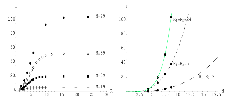
Figure 2: Case 0: $R$ and $M$ dependence for the lifetime. The lines are fits to the data.

3.2.1 $R$ dependence.

We have performed the analysis considering values for the masses of:

$$M^{2}=19,39,59,79.$$ (32)

These values have been chosen in accordance with the previous work [15].

For each of them we have data for a range of values for the radii $R$ starting from the string length $R=\sqrt{\alpha^{\prime}}=2$, up to values sufficiently higher than the threshold $M$.

We fit the dependence of the lifetime on the radii of compactification as in (30). The result shows agreement with the expected power law (28), as can be seen in table (1).

Masses	$\alpha$
$\sqrt{19}=4.36$	1.92231	($2\leq R\leq 3.2$)
$\sqrt{39}=6.24$	1.83862	($2\leq R\leq 5$)
$\sqrt{59}=7.68$	1.9104	($2\leq R\leq 6$)
$\sqrt{79}=8.89$	1.95665	($2\leq R\leq 6$)

Table 1: $R$ dependence for the different masses: ${\cal T}\sim R^{\alpha}$. See the discussion in the text for the uncertainty on $\alpha$.

The values found for $\alpha$ for radii $R<M$ approximate the expected

$$\alpha=d_{c}=2$$ (33)

within the 10% and the agreement is better for the highest mass. Notably (28) is already correct with a good approximation for radii up to values close to the threshold.

Since the dependence on $R$ for small radii of compactification just reproduces the factor $R^{-2}$ which is in front of the amplitude (2.1), this is another confirmation that the contribution to the decay rate of the Kaluza-Klein modes different from zero is suppressed as well as the one of windings.

For radii sufficiently larger than $M$, the dependence on $R$ disappears as expected, with values of $\alpha$ in the range

$$-0.007<\alpha<0.030.$$ (34)

Also for large radii, the main contribution to the decay rate is by the channels with no winding modes and no oscillator modes in both the final states. Therefore, since Kaluza-Klein modes for large radii play the role of components of momenta, we conclude that again the favoured decay is through the emission of a massless and a massive mode.

3.2.2 $M$ dependence.

Since the string lies on extended dimensions only, the contribution to the decay from channels in which there are winding modes is expected to be suppressed. Therefore there are strong motivations for the mass dependence (28) also for small radii.

Indeed the expectation is satisfied up to a reasonably good approximation, as can be seen from table (2).

Range of masses: $4.36<M<8.89$
Radii	$\beta$	Expected value
2	1.42505	1.5
3	1.44265	1.5
4	1.53377	$1.5^{*}$
5	1.5895	$\mbox{}^{*}$
10	2.2036	$\mbox{}^{*}$
16	2.27814	2.5
24	2.28217	2.5

Table 2: $M$ dependence for different radii: ${\cal T}\sim M^{2*\beta}$. (*) indicates cases for which there is no clear expectation of the value of $\beta$ since $R\sim M$ for some of the masses considered.

The differences with the expected values can be accounted for in many ways: from the approximation due to the precision of the number representation in the computer program used, but especially from the considered values of the masses and radii, that are probably not enough to explore the asymptotic limit.

3.3 String lying on one compact and three extended dimensions.

We consider here the configuration in which the string lies on one of the compact dimensions in the space-time background $\mbox{{R}{R}}^{1,7}\times S^{1}\times S^{1}$. The masses taken in account are $M^{2}=19,39,59$, for various values of the compactification radii.

Semi-classical considerations suggest that also in this case the decay rates through winding modes should be suppressed, due to the fact that the Virasoro constraint are less easily satisfied because of the left-right asymmetry of the configuration. Indeed, we have verified that the decays in winding modes give just a very small contribution, sizable only at low masses and radii. We see also that the favoured decay is through the emission of one Kaluza-Klein or massless and one massive states (see table (8), case $dw=1$) and that this last case (massless plus massive final states) prevails for very small radii ($R<<M$). Furthermore, the contribution of decays in massive states with oscillator number different from zero in both the final states is only a negligible fraction of the total, of order $10^{-3}$ for the lowest mass and radii of compactification, down to $10^{-11}$ for the largest mass and radii considered.

We show in figure 3 the $R$ and $M$ dependence of the lifetime.

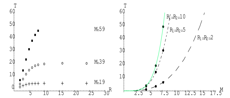
Figure 3: Case I: $R$ and $M$ dependence for the lifetime. The lines are fits to the data.

3.3.1 $R$ dependence.

For radii $R<M$ the dependence (28) is verified with increasingly good approximation at higher masses (around 26.5% of error for small masses, 19.5% for higher ones, see table 3), suggesting that also the Kaluza-Klein contribution to the decay is quite suppressed.

Masses	$\alpha$
$\sqrt{19}=4.36$	1.47213	($2\leq R\leq 4$)
$\sqrt{39}=6.24$	1.55633	($2\leq R\leq 5$)
$\sqrt{59}=7.68$	1.60627	($2\leq R\leq 6$)

Table 3: $R$ dependence for the different masses: ${\cal T}\sim R^{\alpha}$. See the discussion in the text for the uncertainty on $\alpha$.

For radii $R>M$ and masses $M^{2}=19,\,39$ the fit (30) gives values of $\alpha$ in the range

$$0.03<\alpha<0.05,$$ (35)

that is the lifetime is $R$ independent (while for mass $M^{2}=59$ the value found is $\alpha=0.33887,$ that can be explained noticing that the values of the radii considered are not so larger than the threshold).

3.3.2 $M$ dependence.

The broad qualitative picture for the mass dependence of the lifetime is similar to the expected (28) but the transition between $\beta=1.5$, (expected for small radii) and $\beta=2.5$ (expected for large radii) is less sharp than in the case of the string lying on extended dimensions for the data $R<M$ (see table (4)).

Range of masses: $4.36<M<7.68$
Radii	$\beta$	Expected value
2	1.56233	1.5
3	1.64233	1.5
4	1.774497	$\mbox{}^{*}$
5	1.90883	$\mbox{}^{*}$
10	2.212286	$2.5$

Table 4: $M$ dependence for different radii: ${\cal T}\sim M^{2*\beta}$. (*) indicates cases for which there is no clear expectation of the value of $\beta$ since $R\sim M$ for some of the masses considered.

This is due to the increasing contribution for higher radii by the channels of decay into Kaluza-Klein modes (plus a massive final state).

The trend towards the asymptotic pattern is clear, even though our analysis could only consider limited values of masses and radii.

3.4 String lying on two extended and two compact dimensions.

In this section we will consider a string lying on both the compact dimensions of the space-time background $\mbox{{R}{R}}^{1,7}\times S^{1}\times S^{1}$, with say $X^{1}$ on one $S^{1}$ and $X^{3}$ on the other $S^{1}$ and $X^{2,4}$ on $\mbox{{R}{R}}^{7}$. Here we expect a substantial contribution of the winding modes to the decay, since the string can wind with both chiralities.

This has been the most difficult case to be studied: the number of computer processes needed to calculate the imaginary part of the amplitude (formula (20)) is very high. Furthermore increasing the values of the masses implies working with very large numbers. Consequently our analysis has been limited to values for the masses of:

$$M^{2}=19,29,39,59$$ (36)

and to a restricted range of radii (in the case of $M^{2}=59$ only a few data could be obtained).

As we said, in this case the decay through winding modes is possible, and for small radii (compared to the string length) we expect it is the favorite decay. Table (8) proves this claim for all the mass tested: for $R<M$ the decay channels without windings give a small fraction of the total rate, for $R\geq M$, on the contrary, their contribution dominates.

Figure 4: Case II: $R$ and $M$ dependence for the lifetime.The lines are fits to the data.

3.4.1 $R$ dependence.

The power law (28) is not correct for radii $R<M$: the decay rate is much more rapid for very small radii due to a dominant contribution from channels of decay in winding modes, but this contribution decreases rapidly to a negligible fraction of the total rate of decay when increasing the radii.

We have reported in figure 4a the lifetime at fixed $M$ for various $R$.

For radii $R>M$, instead, as expected, the lifetime is flat with respect to the radii.

3.4.2 $M$ dependence.

Due to the dominant contributions of the decays through winding modes, the expected power law (28) is not correct for $R<M$. The lifetime is almost flat or slightly increases for higher masses, and it does not exhibit a power law dependence on mass, as can be seen in figure 4b.

For $R>M$, instead, the mass dependence of the lifetime tends to agreement with (28), although we could test it only for radii just above the threshold and for squared masses $M^{2}=19,\,29,\,39$:

Range of masses: $4.36<M<6.24$
Radii	$\beta$	Expected value
7	2.11488	2.5
8	2.16404	2.5

Table 5: $M$ dependence for different radii: ${\cal T}\sim M^{2*\beta}$.

3.5 Comparison of the various cases with each other.

In this section we will discuss the results found for the decay rates comparing the likelihood for the string to decay in the different cases 0, I, II, defined in section 3.1. In all the above cases two out of the nine space dimensions are compactified on circles with the same radius $R_{1}=R_{2}=R$.

We would expect that if the string lies on the compactified dimensions and therefore has the possibility to wrap on them (if the radii of the compact dimensions are smaller than the string length), the decay should be enhanced, unless the Virasoro constraints make it difficult. For larger radii, instead, there shouldn’t be any appreciable difference in the decay rates, since for all the string configuration they should tend to the flat space value.

We have computed the ratio between the values for the decay rates in the various cases at corresponding masses and radii, see table (6).

The results show that for radii $R>M$ the decay rates tend to the same value (the flat space-time one). Let us analyze the behaviour for small radii $R<M$.

The rate for case II is the largest one, with respect to both configurations I and 0. Furthermore the ratio increases for higher masses at fixed radii. This is expected, since the decay rates for the string in configuration I or 0 decreases with a power law as $\mathcal{R}\sim M^{-1.5}$ , whereas the one for the string lying on two compact dimensions decreases in a less marked way (see figure (4) and tables (9-8), the rate is the inverse of the lifetime).

On the contrary the ratio between the decay rate for cases I and 0 shows, that in the first case (I), the string decays less. This can be accounted by the fact that the string constraints $\dot{X}+X^{\prime}=0,\,\dot{X}\cdot X^{\prime}=0$ are less easily satisfied in the more asymmetric configuration of the string lying on one compact dimension only.

Mass $M=4.36$
Radii	$II/0$	$I/0$	$II/I$
2	4.23898	0.732018	5.79082
3	4.04003	0.811177	4.98046
4	1.05918	0.914973	1.15761
5	0.974573	0.972415	1.00222
6	1.01443	1.00094	1.01348
7	0.999821	1.00312	0.996712
8	1.02703	1.01037	1.01649
Mass $M=6.24$
Radii	$II/0$	$I/0$	$II/I$
2	8.91015	0.641493	13.8897
3	9.42839	0.685099	13.7621
4	13.0199	0.777693	16.7417
5	2.47845	0.869407	2.85074
6	0.911707	0.943306	0.966502
7	0.975422	0.975233	1.00019
8	1.01423	0.994766	1.01956
Mass $M=7.68$
Radii	$II/0$	$I/0$	$II/I$
2	13.7567	0.624082	22.0431
4	21.2468	0.709832	18.5974

Table 6: Decay rates comparison for some fixed mass and radii. II means string lying on two compact dimensions with opposite chiralities. I means string lying on one compact dimension. 0 means string lying on extended dimensions only.

4 Summary of the results and conclusions.

We have studied the decay of a particular closed string state of type II string theory that in a previous work ([15]) was shown to be long-lived in ten uncompactified flat dimensions. It classically corresponds to the string configuration of equation (1).

We have considered a space-time $\mbox{{R}{R}}^{1,7}\times T^{2}$ and chosen three string configuration:

• 0: string lying on extended dimensions only;

• I: string lying on three extended and one compact dimension;

• II: string lying on two extended and two compact dimensions, with opposite chirality.

Throughout all the paper we have considered $R_{1}=R_{2}=R$, but we have also data (not shown) for $R_{1}\neq R_{2}$.

In case 0, the string decay is entirely given by the emission of a massless plus a massive final state. The difference between this and the ten flat uncompactified dimensions case lies only in the reduced phase-space factor when the radii of compactification are small.

The string in configuration I decays in one massless and one massive state for $R<<M$. For $R\sim M$, the other dominant decay channel is through one Kaluza-Klein plus one massive final state. This channel becomes the most important for $R>M$, where the total decay rate flattens as expected and the Kaluza-Klein modes play the role of momentum components. The winding modes do not seem to play a significant role at any radius.

Finally, in case II the string shows the most rapid and intense decay for small radii. The winding modes channels dominate. For $R<M$ the lifetime slightly increases by increasing the parent mass (at fixed radii) and by increasing the radii $R<M$ (at fixed mass). For $R>M$ we recover the uncompactified dimensions result.

In all the cases the threshold separating the behaviour at large radii (lifetimes $\mathcal{T}\sim g_{s}M^{5}$ and no dependence on $R$, as in the uncompactified scenario) from the behaviour at small radii ($\mathcal{T}$ increasing more slowly) is found to be $R\sim M$.

The above results confirm the general expectations on the effect of compactification on the decay properties of the string state we have considered. Although we have examined in detail the case in which two of the nine space dimensions of the theory are compact, the decay pattern can be clearly extrapolated to the case of compactification of additional dimensions.

Our conclusion is that the string configuration we have studied is generally long lived. The lifetime increases with the mass, at least when its size is smaller than the radius of the dimensions it lies on, and even for larger sizes, if it lies in part on the uncompact space and it does not wind with opposite chiralities on the compact dimensions. The dominant decay channel is the soft emission of massless states.

5 Acknowledgments

Partial support by the EEC Network contract HPRN-CT-2000-00131 and by the Italian MIUR program “Teoria dei Campi, Superstringhe e Gravità” is acknowledged.

Appendix A Appendix A: Computation of ${\rm Im}(\Delta M^{2})$

In these appendices we explain in details the computations needed to obtain the imaginary part of amplitude (7) shown in section (2).

We have always taken two space-time coordinates as compactified on a torus, while all the others were not. It means that we identify points of the two compactified dimensions under the action of the group of translation generated by the element

$$v=2\pi R$$ (37)

so that the bosonic coordinates transform as

$$X^{\mu}=X^{\mu}+mv,\quad m\,\epsilon\,\mbox{{Z}{Z}},$$ (38)

the fermionic

$$\psi^{\mu}=\psi^{\mu}$$ (39)

and the resulting space-time is:

$$\mbox{{R}{R}}^{8}\times T^{2}.$$

This implies that the fermionic propagator is unchanged and still obeys the Riemann identity, the bosonic one, instead, is different depending on if the string lies or not on the compactified coordinates.

This propagator can be computed trough path integral formalism.

A.1 String lying on extended dimensions only.

The propagator for the string coordinates in this case is the same as in the uncompactified scenario:

$$\langle\partial\bar{Z}_{i}(z)\partial Z_{j}(0)\rangle=\delta_{ij}\ 2\left(\partial^{2}\log\theta_{1}(z|\tau)+{\pi\over\tau_{2}}\right)\ ,$$

$$\langle\bar{\partial}\bar{Z}_{i}(z)\bar{\partial}Z_{j}(0)\rangle=\delta_{ij}\ 2\left(\bar{\partial}^{2}\log\bar{\theta}_{1}(z|\tau)+{\pi\over\tau_{2}}\right)\,$$

$$\langle\bar{\partial}\bar{Z}_{i}(z)\partial Z_{j}(0)\rangle=\langle\partial\bar{Z}_{i}(z)\bar{\partial}Z_{j}(0)\rangle=-\delta_{ij}2\ {\pi\over\tau_{2}}\ ,$$

$$\langle e^{-ipX(z)}e^{ipX(0)}\rangle=e^{-4N{\pi y^{2}\over\tau_{2}}}\ \left|{\theta_{1}(z|\tau)\over\theta_{1}^{{}^{\prime}}(0|\tau)}\right|^{4N}$$ (40)

(here $y={\rm Im}(z)$).

What changes is the integral over the zero modes (here not only momenta, but also winding modes) giving us a final measure of integration for $\tau$

$$\int\frac{d^{2}\tau}{\tau_{2}^{4}}\prod_{i=1}^{2}\left({1\over\sqrt{\pi\tau_{2}}}\sum_{l_{i},w_{i}}e^{-\frac{\pi R^{2}}{4\tau_{2}}|l_{i}-m_{i}\tau|^{2}}\right)$$ (41)

where $l_{i},\,m_{i}$ are winding modes.

The correlator in (7) is:

$$\langle\bar{V}_{k,k}(z)V_{k,k}(0)\rangle =$$

$$= {N^{2}\over 4^{N-1}((N-1)!)^{2}}\langle\langle e^{-ipX(z)}e^{ipX(0)}\rangle$$

$$\times \psi_{\bar{z}_{1}}(z)\partial\psi_{\bar{z}_{1}}(z)\tilde{\psi}_{\bar{z}_{2}}(z){\bar{\partial}}\tilde{\psi}_{\bar{z}_{2}}(z)\psi_{z_{1}}(0)\partial\psi_{z_{1}}(0)\tilde{\psi}_{z_{2}}(0){\bar{\partial}}\tilde{\psi}_{z_{2}}(0)\rangle$$

$$\times \langle(\partial\bar{Z}_{1}(z))^{N-1}(\partial Z_{1}(0))^{N-1}({\bar{\partial}}\bar{Z}_{2}(z))^{N-1}({\bar{\partial}}Z_{2}(0))^{N-1}\rangle$$

giving, from (A.1) and

$$\langle(\partial\bar{Z}_{1})^{N-1}(\partial Z_{1})^{N-1}\rangle=(N-1)!\delta_{ij}\ 2\left(\partial^{2}\log\theta_{1}(z|\tau)+{\pi\over\tau_{2}}\right),$$ (43)

the result:

$$\langle\bar{V}_{k,k}(z)V_{k,k}(0)\rangle=(N)^{2}\langle e^{-ipX(z)}e^{ipX(0)}\rangle\left|\partial^{2}\log\theta_{1}(z|\tau)+{\pi\over\tau_{2}}\right|^{2(N-1)}$$ (44)

as in [15].

We expand then the holomorfic and antiholomorfic factors in binomials, obtaining:

$$\langle\bar{V}_{k,k}(z)V_{k,k}(0)\rangle=(N)^{2}\langle e^{-ipX(z)}e^{ipX(0)}\rangle({\pi\over\tau_{2}})^{2(N-1)}$$ (45)

$$\times\sum_{m_{1},m_{2}}\big{(}{\pi\over\tau_{2}}\big{)}^{-m_{1}-m_{2}}\mbox{\small{$\frac{((N-1)!)^{2}}{m_{1}!m_{2}!(N-1-m_{1})!(N-1-m_{2})!}$}}\big{(}\partial^{2}\log(\theta_{1}(z|\tau)\big{)}^{m_{1}}\big{(}\bar{\partial}^{2}\log(\theta_{1}(z|\tau)\big{)}^{m_{2}}\ .$$

We perform a Poisson re-summation on the sum over $l_{i}$ in (41) so that we obtain the final amplitude (2.1).

A.2 String lying on one compactified dimensions.

In this case, coordinate $X^{1}$ is compactified (together with another coordinate, where the string does not lies).

According to (3) for the correlator $\langle\bar{V}V\rangle$ we need in particular the part

$$\langle\partial X^{1}(z_{1})\partial X^{1}(z_{2})\rangle=$$ (46)

$$\sum_{m,l}\int_{\begin{subarray}{c}X^{1}(z+1)=X^{1}(z)+2\pi Rm\\ X^{1}(z+\tau)=X^{1}(z)+2\pi Rl\end{subarray}}\mathcal{D}X^{1}e^{-S[X^{1},\tau]}\partial X^{1}(z_{1})\partial X^{1}(z_{2})$$

To compute this path-integral we can split the coordinate $X^{1}(z)$ in a classical part, obeying the boundary conditions, and a periodical quantum part

$$X^{1}(z)=X^{1}_{cl}(z)+X^{1}_{qu}(z)$$ (47)

where

$$X^{1}_{cl}(z)=\frac{\pi R}{i\tau_{2}}(l-m{\bar{\tau}})z-\frac{\pi R}{i\tau_{2}}(l-m\tau)\bar{z}$$ (48)

In terms of the complex coordinates (49), we write

$$\begin{cases}\partial Z_{1}(z)&=\partial Z_{1}^{0}(z)+{\alpha\over\sqrt{2}}\\ \partial\bar{Z}_{1}(z)&=\partial\bar{Z}_{1}^{0}(z)+{\alpha\over\sqrt{2}}\\ \end{cases}$$ (49)

where

$$\alpha={\pi R_{1}\over i\tau_{2}}(l-m{\bar{\tau}})$$ (50)

and $\partial Z_{1}^{0}(z)$ is the oscillator part of the string coordinate expansion.

The correlator is again given by (A.1), but now equations (49) lead to:

$$\langle(\partial\bar{Z}_{1})^{N-1}(\partial Z_{1})^{N-1}\rangle = \langle\left(\partial\bar{Z}^{0}_{1}+{\alpha\over\sqrt{2}}\right)^{N-1}\left(\partial Z^{0}_{1}+{\alpha\over\sqrt{2}}\right)^{N-1}\rangle=$$ (51)

$$= \sum_{s_{1},s_{2}=0}^{N-1}\mbox{\tiny{$\left(\begin{array}[]{c}N-1\\ s_{1}\end{array}\right)\left(\begin{array}[]{c}N-1\\ s_{2}\end{array}\right)$}}\langle\partial\bar{Z}_{1}^{0}(z)^{N-1-s_{1}}\partial Z_{1}^{0}(0)^{N-1-s_{2}}\rangle$$

$$\times \left({\alpha\over\sqrt{2}}\right)^{s_{1}}\left({\alpha\over\sqrt{2}}\right)^{s_{2}}$$

so that the result is:

$$\langle\bar{V}(z)V(0)\rangle =$$ (57)

$$= {N^{2}\over 4^{N-1}((N-1)!)^{2}}\sum_{s_{1},s_{2}=0}^{N-1}\mbox{\tiny{$\left(\begin{array}[]{c}N-1\\ s_{1}\end{array}\right)\left(\begin{array}[]{c}N-1\\ s_{2}\end{array}\right)$}}$$

$$\times \langle\partial\bar{Z}_{1}^{0}(z)^{N-1-s_{1}}\partial Z_{1}^{0}(0)^{N-1-s_{2}}\rangle\left({\alpha\over\sqrt{2}}\right)^{s_{1}}\left({\alpha\over\sqrt{2}}\right)^{s_{2}}$$

$$\times \langle{\bar{\partial}}\bar{Z}_{2}^{0}(z)^{N-1}{\bar{\partial}}Z_{2}^{0}(0)^{N-1}\rangle e^{-4N{\pi y^{2}\over\tau_{2}}}\left|{\theta_{1}(z|\tau)\over\theta_{1}^{{}^{\prime}}(0|\tau)}\right|^{4N}$$

The non-vanishing part of the amplitude is the one with $s_{1}=s_{2}=s$. Using, then, formulas (A.1) for the correlator of the oscillator part of the string coordinate and (41) for the measure of integration, we arrive to the result:

$$\Delta M^{2} = c^{\prime}\ g_{s}^{2}\ \int{d^{2}\tau\over\tau_{2}^{4}}\int d^{2}z\sum_{l_{1,2},w_{1,2}}\sum_{s=0}^{N-1}\sum_{m_{1}=0}^{N-1-s}\sum_{m_{2}=0}^{N-1}\mbox{\small{${N^{2}((N-1)!)^{2}\over(s!)^{2}m_{1}!m_{2}!(N-1-s-m_{1})!(N-1-m_{2})}$}}$$

$$\times \left({\pi\over\tau_{2}}\right)^{2N-2}\left(-{\pi R_{1}^{2}\over 4\tau_{2}}(l_{1}-w_{1}\bar{\tau})^{2}\right)^{s}\left({\tau_{2}\over\pi}\partial^{2}\log\theta_{1}(z|\tau)\right)^{m_{1}}\left({\tau_{2}\over\pi}{\bar{\partial}}^{2}\log\bar{\theta}_{1}(\bar{z}|\bar{\tau})\right)^{m_{2}}$$

$$\times e^{-4N{\pi y^{2}\over\tau_{2}}}\left|{\theta_{1}(z|\tau)\over\theta_{1}^{{}^{\prime}}(0|\tau)}\right|^{4N}\frac{1}{\pi\tau_{2}}e^{-{\pi\over 4\tau_{2}}R_{1}^{2}|l_{1}-w_{1}\tau|^{2}-{\pi\over 4\tau_{2}}R_{2}^{2}|l_{2}-w_{2}\tau|^{2}}$$

Now consider:

$$A_{R}=\sum_{l_{1}}\sum_{s}\left({\pi R_{1}^{2}\over 4\tau_{2}}(l_{1}-w_{1}\bar{\tau})^{2}\right)^{s}e^{-{\pi\over 4\tau_{2}}R_{1}^{2}|l_{1}-w_{1}\tau|^{2}},$$ (64)

where the subscript $R$ refers to the fact the this concerns the right moving part of the string only.

Call

$$a={\pi R_{1}^{2}\over 4\tau_{2}}.$$ (65)

We can write:

$$A_{R} = \sum_{l_{1}}\sum_{s}\left(a(l_{1}-w_{1}\bar{\tau})^{2}\right)^{s}e^{-a|l_{1}-w_{1}\tau|^{2}}$$

$$= \left.\sum_{l_{1}}\sum_{s}(-\partial_{b})^{s}e^{-a|l_{1}-w_{1}\tau|^{2}-ba(l_{1}-w_{1}\bar{\tau})^{2}}\right|_{b=0}.$$

Now perform a Poisson re-summation on $l_{1}$:

$$A_{R} = \left.\sum_{l_{1}}\sum_{s}(-\partial_{b})^{s}e^{-a|l_{1}-w_{1}\tau|^{2}-ba(l_{1}-w_{1}\bar{\tau})^{2}}\right|_{b=0}$$

$$= \left.\sum_{n_{1}}\sum_{s}\sqrt{{\pi\over a}}(-\partial_{b})^{s}\sqrt{{1\over 1+b}}e^{-{\pi^{2}\over a(1+b)}\left(n_{1}+{aw_{1}\tau_{2}\over\pi}\right)^{2}+2i\pi\tau_{1}n_{1}w_{1}+2\pi w_{1}\tau_{2}n_{1}}\right|_{b=0}.$$

We have got to compute

$$P=\sum_{s}(-\partial_{b})^{s}\sqrt{{1\over 1+b}}e^{-{\pi^{2}\over a(1+b)}\left(n_{1}+{aw_{1}\tau_{2}\over\pi}\right)^{2}}.$$ (68)

Calling therefore $y={1\over 1+b}$ it can be shown that

$$\sum_{s}(-\partial_{b})^{s}=\sum_{s}(y^{2}\partial_{y})^{s}=\sum_{s}\sum_{l=1}^{s}c_{s}^{l}y^{l+s}\partial_{y}^{l}$$ (69)

where the coefficients $c_{s}^{l}$ are defined recursively as

$$\begin{cases}c_{s}^{l}&=c_{s-1}^{l}(l+s-1)+c_{s-1}^{l-1}\\ c_{s}^{l}&=0,\,s<l\\ c_{s}^{1}&=s!\,s\neq 0\\ c_{s}^{0}&=0,\,s\neq 0\\ c_{0}^{0}&=1\\ \end{cases}$$

so that

$$P=\sum_{s}\sum_{l=0}^{s}c_{s}^{l}\sum_{r=0}^{l}\mbox{\small{$\left(\begin{array}[]{c}l\\ r\end{array}\right)$}}{\Gamma(3/2)\over\Gamma(3/2-l+r)}\,e^{-{4\pi\tau_{2}\over R_{1}^{2}}\left(n_{1}+{w_{1}R_{1}^{2}\over 4}\right)^{2}}\left(-{4\pi\tau_{2}\over R_{1}^{2}}\left(n_{1}+{w_{1}R_{1}^{2}\over 4}\right)^{2}\right)^{r}.$$ (70)

Inserting this result in (A.2), performing a Poisson re-summation also on $l_{2}$ and expanding again the relevant terms as in (10), we get an imaginary part for the mass shift as shown in equation (2.2).

A.3 String lying on two compactified dimensions.

In this case we have compactified both coordinates $X^{1}$ and $X^{3}$. For the Right-moving part of the string, the contribute to the amplitude is the same as the Right moving part discussed in the previous section. For what concerns instead the Left-moving sector, the computation is analogous, substituting

$$A_{L}=\sum_{l_{2}}\sum_{s}\left({\pi R_{2}^{2}\over 4\tau_{2}}(l_{2}-w_{2}\tau)^{2}\right)^{s}e^{-{\pi\over 4\tau_{2}}R_{2}^{2}|l_{2}-w_{2}\tau|^{2}}$$ (71)

to (64).

With the same steps as in the previous computation, eventually we obtain:

$$A_{L} = \sum_{n_{2}}\sum_{s}\sum_{l=0}^{s}c_{s}^{l}\mbox{\small{$\left(\begin{array}[]{c}l\\ r\end{array}\right)$}}{\Gamma(3/2)\over\Gamma(3/2-l+r)}\,$$ (74)

$$\times e^{-{4\pi\tau_{2}\over R_{2}^{2}}\left(n_{2}-{w_{2}R_{2}^{2}\over 4}\right)^{2}+2i\pi\tau_{1}w_{2}n_{2}-2\pi\tau_{2}w_{2}n_{2}}\left(-{4\pi\tau_{2}\over R_{2}^{2}}\left(n_{2}-{w_{2}R_{2}^{2}\over 4}\right)^{2}\right)^{r}.$$ (75)

The imaginary part of the amplitude is, then, shown in equation (20).

Appendix B Appendix B: Tables

We report here a selection of the data.

$M$	$R1=R2=R$	$dw=0$	$dw=1$
$\sqrt{19}=4.36$	$2$	$1.2172\,(1.2167)$	$0.89104\,(0.81904)$
$\sqrt{19}=4.36$	$4$	$0.35470\,(0.35465)$	$0.32454\,(0.32345)$
$\sqrt{19}=4.36$	$8$	$0.25114\,(0.25109)$	$0.25374\,(0.25369)$
$\sqrt{19}=4.36$	$16$	$0.24990(0.24985)$	$0.24963(0.24959)$
$\sqrt{39}=6.24$	$2$	$0.44313\,(0.44313)$	$0.28427\,(0.28057)$
$\sqrt{39}=6.24$	$4$	$0.11406\,(0.11406)$	$0.088708\,(0.088681)$
$\sqrt{39}=6.24$	$8$	$0.053780\,(0.053779)$	$0.05350\,(0.053498)$
$\sqrt{39}=6,24$	$16$	$0.050159\,(0.050159)$	$0.050175\,(0.050175)$
$\sqrt{59}=7.68$	$2$	$0.24404\,(0.24404)$	$0.15230\,(0.15177)$
$\sqrt{59}=7.68$	$4$	$0.061474\,(0.061474)$	$0.043636\,(0.043635)$
$\sqrt{59}=7.68$	$8$	$0.022650\,(0.022650)$	$0.0218738\,(0.2187)$
$\sqrt{59}=7.68$	$16$	$0.01919(0.019187)$	$(0.2496)$

Table 7: Decay Rates for two compact dimensions ($dw$=number of compact dimensions where the string lies): - numbers not enclosed in brackets represent the total decay rate, - numbers in round brackets ($\dotsc$) represent the contribution of channels where one of the two decay products is a pure Kaluza-Klein mode. Actually, for small radii the decay in non-zero Kaluza-Klein modes represents only less than 0.5% of the total decay for large masses in the case $dc=2,\,dw=0$ and between the 0.6% and 13% for the case $dc=2,\,dw=1$.

$M$	$R1=R2=R$	$dw=2$
$\sqrt{19}=4.36$	$2$	$5.1598\,\{0.66702\}$
$\sqrt{19}=4.36$	$4$	$0.37569\,\{0.30917\}$
$\sqrt{19}=4.36$	$8$	$0.25793\,\{0.25793\}$
$\sqrt{39}=6.24$	$2$	$3.9484\,\{0.22226\}$
$\sqrt{39}=6.24$	$4$	$1.4851\,\{0.077970\}$
$\sqrt{39}=6.24$	$8$	$0.054544\,\{0.054544\}$
$\sqrt{59}=7.68$	$2$	$3.3572\,\{0.11935\}$
$\sqrt{59}=7.68$	$4$	$1.3061$

Table 8: Decay Rates for two compact dimensions (here $dw$=number of compactified dimensions where the string lies=2): - numbers not enclosed in brackets represent the total decay rate, - numbers in curly brackets {$\dotsc$} represent the contribution of channels with zero winding modes.

$M$	$R1=R2=R$	$dw=0$	$dw=1$	$dw=2$
$\sqrt{19}=4.36$	$2$	$0.82153$	$1.1223$	$0.19380$
$\sqrt{19}=4.36$	$4$	$2.8193$	$3.0813$	$2.6617$
$\sqrt{19}=4.36$	$8$	$3.9819$	$3.9410$	$3.8771$
$\sqrt{19}=4.36$	$16$	$4.0017$	$4.0058$
$\sqrt{39}=6.24$	$2$	$2.2566$	$3.5178$	$0.25327$
$\sqrt{39}=6.24$	$4$	$8.7669$	$11.2729$	$0.67335$
$\sqrt{39}=6.24$	$8$	$18.594$	$18.6924$	$18.334$
$\sqrt{39}=6.24$	$16$	$19.936$	$19.930$
$\sqrt{59}=6.24$	$2$	$4.0977$	$6.5660$	$0.29787$
$\sqrt{59}=6.24$	$4$	$16.267$	$22.9169$	$0.76563$
$\sqrt{59}=6.24$	$8$	$44.150$	$45.7167$
$\sqrt{59}=6.24$	$16$	$52.118$

Table 9: Values of the lifetime for two compact dimensions. ($dw$=number of compact dimensions where the string lies)

References

- [1] E. J. Copeland, R. C. Myers and J. Polchinski, arXiv:hep-th/0312067.
- [2] M. G. Jackson, N. T. Jones and J. Polchinski, arXiv:hep-th/0405229.
- [3] M. B. Green and G. Veneziano, “Average Properties Of Dual Resonances,” Phys. Lett. B 36, 477 (1971).
- [4] D. Mitchell, N. Turok, R. Wilkinson and P. Jetzer, “The Decay Of Highly Excited Open Strings,” Nucl. Phys. B 315, 1 (1989) [Erratum-ibid. B 322, 628 (1989)].
- [5] J. Dai and J. Polchinski, “The Decay Of Macroscopic Fundamental Strings,” Phys. Lett. B 220, 387 (1989).
- [6] H. Okada and A. Tsuchiya, “The Decay Rate Of The Massive Modes In Type I Superstring,” Phys. Lett. B 232, 91 (1989).
- [7] B. Sundborg, “Selfenergies Of Massive Strings,” Nucl. Phys. B 319, 415 (1989).
- [8] R. B. Wilkinson, N. Turok and D. Mitchell, “The Decay Of Highly Excited Closed Strings,” Nucl. Phys. B 332, 131 (1990).
- [9] D. Mitchell, B. Sundborg and N. Turok, “Decays Of Massive Open Strings,” Nucl. Phys. B 335, 621 (1990).
- [10] D. Amati and J. G. Russo, “Fundamental strings as black bodies,” Phys. Lett. B 454, 207 (1999) [arXiv:hep-th/9901092].
- [11] R. Iengo and J. Kalkkinen, “Decay modes of highly excited string states and Kerr black holes,” JHEP 0011, 025 (2000) [arXiv:hep-th/0008060].
- [12] J. L. Manes, “Emission spectrum of fundamental strings: An algebraic approach,” Nucl. Phys. B 621, 37 (2002) [arXiv:hep-th/0109196].
- [13] R. Iengo and J. G. Russo, “The decay of massive closed superstrings with maximum angular momentum,” JHEP 0211, 045 (2002) [arXiv:hep-th/0210245].
- [14] R. Iengo and J. G. Russo, “Semiclassical decay of strings with maximum angular momentum,” JHEP 0303, 030 (2003) [arXiv:hep-th/0301109].
- [15] D. Chialva, R. Iengo and J. G. Russo, “Decay of long-lived massive closed superstring states: Exact results,” JHEP 0312 (2003) 014 [arXiv:hep-th/0310283].
- [16] A. Hashimoto and I. R. Klebanov, Nucl. Phys. Proc. Suppl. 55B, 118 (1997) [arXiv:hep-th/9611214].
- [17] N. Lambert, H. Liu and J. Maldacena, arXiv:hep-th/0303139.
- [18] I. Antoniadis, arXiv:hep-th/0102202.