Phantom Inflation and the ”Big Trip”

Abstract

Primordial inflation is regarded to be driven by a phantom field which is here implemented as a scalar field satisfying an equation of state $p=\omega\rho$, with $\omega<-1$. Being even aggravated by the weird properties of phantom energy, this will pose a serious problem with the exit from the inflationary phase. We argue however in favor of the speculation that a smooth exit from the phantom inflationary phase can still be tentatively recovered by considering a multiverse scenario where the primordial phantom universe would travel in time toward a future universe filled with usual radiation, before reaching the big rip. We call this transition the ”big trip” and assume it to take place with the help of some form of anthropic principle which chooses our current universe as being the final destination of the time transition.

PACS: 04.60.-m, 98.80.Cq

Keywords: Phantom energy, Inflation, Wormholes

Phantom energy might be currently dominating the universe. This is a possibility which is by no means excluded by present constraints on the universal equation of state [1]. If phantom energy currently dominated over all other cosmic components in the universe, then we were starting a period of super-accelerated inflation which would even be more accelerated than the accelerating process that corresponded to the existence of a positive cosmological constant. One could thus be tempted to look at the primordial inflation as being originated by a phantom field. In fact, Piao and Zhang have already considered [2] an early-universe scenario where the inflationary mechanism is driven by phantom energy. The main difficulty with that scenario is that it is difficult to figure out in it how the universe can smoothly exit from the inflationary period, as an inflating phantom universe seems to inexorably ends up in a catastrophic big rip singularity. Now, however, we seem to have a tool which might help to solve that difficulty. It is based on the rather astonishing effects that accretion of phantom energy can induce in the evolution of Lorentzian wormholes [3].

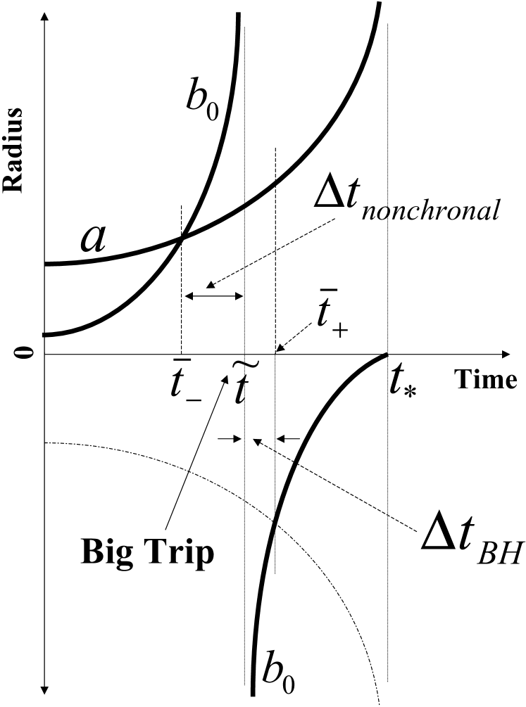
Figure 1: Evolution of the radius of the wormhole throat, $b_{0}$, induced by accretion of phantom energy. At time $t=\tilde{t}$, the negative exotic mass becomes infinite and then changes sign, so converting the wormhole into an Einstein-Rosen bridge whose associated mass decreases down to zero at the big rip at $t=t_{*}$. During the time interval $\Delta t_{nonchronal}$ there will be a disruption of the causal evolution of the whole universe. The evolution of the phantom universe at time $t=\tilde{t}$ is fully noncausal and all sorts of time travel are then allowed. Therefore the moment at $t=\tilde{t}$ is here dubbed as the ”Big Trip”.

Since phantom energy violates dominant energy condition, wormholes can naturally occur [4] in a universe dominated by phantom energy [5]. It can in fact be thought that if Planck-sized wormholes are quantum-mechanically stable and were also allowed to exist in the primordial spacetime foam of a phantom dominated early universe, then before occurrence of the big rip [6], the throat of the wormholes will rapidly increase and become larger than the size of the inflating universe itself, to blow up before the big rip [3]. The moment at which all the originally Planck-sized wormholes of the spacetime foam become simultaneously infinite could thus be dubbed as the ”Big Trip” (Fig. 1), as a sufficiently inflated early universe would then be inside the throat of the wormholes and could thus be itself converted into a ”time traveller” which may be instantly transferred either to its past or to its future. Conditions for the Big Trip does not just occur at the time when the size of the wormhole throat blows up, but they extend backwards, down to the time at which the wormhole throat size just overcomes the phantom universe size, all the way along the time interval $\Delta T_{nonchronal}$ shown in Fig. 1.

In what follows we shall implement the above picture by using a semi-quantitative scenario where we first describe how a set of parallel quantum universes (which would include both the phantom universe and a universe filled with usual radiation) can be quantum-mechanically derived, and then discuss the way through which a time travel from the phantom universe to the Friedmann universe with usual radiation may lead to a smooth exit from inflation taking place in the former universe. Let us thus consider the spacetime manifold $M$ for a little flat FRW universe with metric

$$ds^{2}=-N^{2}dt^{2}+a(t)d\Omega_{3}^{2},$$ (1)

where $N$ is the lapse function resulting from foliating the manifold $M$, $d\Omega_{3}^{2}$ is the metric on the unit three-sphere, and $a(t)$ is the scale factor. Such a universe will be filled with dark energy and equipped with a general equation of state $p=\omega\rho$, where $\omega$ is a parameter which is here allowed to be time-dependent. We shall then formulate the quantum-mechanical description of such a universe starting with its action integral. For this we shall take the most general Hilbert-Einstein action where, besides considering the scale factor $a(t)$ and the scalar field $\phi(t)$ to be time-dependent, and hence appearing in the action as a given combination of $a$, $\phi$, $\dot{a}$ and $\dot{\phi}$ (with $\dot{}=d/dt$), we will generally regard the state equation parameter $\omega$ to be initially time-dependent, too, even though we restrict ourselves to the case where we always have $\ddot{\omega}=0$.

Differentiating then the Friedmann equation (i.e. Eq. (14) below which will be in principle defined for a flat FRW universe with constant $\omega$) with respect to time one can see that, if the $\omega$ in that equation is nevertheless regarded to be time-dependent then the scalar curvature can be generalized to a new expression $\hat{R}$ which thereby is suggested to be given by

$$\hat{R}=R-\frac{\dot{a}\dot{\omega}\ln a^{9}}{a},$$

where $R$ is the conventional Ricci curvature scalar. In obtaining this expression we have first assumed $\rho=\rho_{0}a^{-3(1+\omega)}$, letting then $\omega\equiv\omega(t)$ in it. Thus, since the scalar curvature for a flat universe is given by $6(\ddot{a}+\dot{a}^{2}/a^{2})$, it can be checked that differentiation of Eq. (14) directly produces the extra term appearing in the expression for $\hat{R}$. To this generalized Ricci curvature scalar one should then associate a correspondingly generalized extrinsic curvature $\hat{K}$. In such a case the action integral of the manifold $M$ with boundary $\partial M$ can be written as

$$S=\int_{M}d^{4}x\sqrt{-g}\left(\frac{\hat{R}}{16\pi G}+L_{\phi}\right)-\frac{1}{8\pi G}\int_{\partial M}d^{3}x\sqrt{-h}Tr\hat{K}$$

$$=\int_{M}d^{4}x\sqrt{-g}\;[\frac{1}{16\pi G}\left(R-\frac{\dot{a}\dot{\omega}\ln a^{9}}{aN^{2}}\right)+\frac{1}{2}(\partial_{\mu}\phi)^{2}-V(\phi)]$$

$$-\frac{1}{8\pi G}\int_{\partial M}d^{3}x\sqrt{-h}\;\left(TrK-\frac{\dot{\omega}\ln a^{3/2}}{N}\right),$$ (2)

in which $K$ is the conventional expression for the extrinsic curvature, and $g$ and $h$ denote, respectively, the determinants of the general four-metric $g_{ij}$ on $M$ and three-metric $h_{ij}$ on the given hypersurface at the boundary $\partial M$, characterized by a lapse $N$ and a shift $N_{i}$ functions. We note that (i) the above action integral becomes the conventional Hilbert-Einstein action for $\omega$=Const., (ii) in the surface integral we have also added a new non-conventional extra term depending on $\dot{\omega}$ which would represent a transition between different universes each with a fixed equation of state, and together with $TrK$ would make the trace of the generalized extrinsic curvature $Tr\hat{K}$, and finally that (iii) the momenta conjugate to $a(t)$ and $\omega(t)$ are not separable from each other even when we have assumed $\ddot{\omega}=0$. In the case that we consider that, in principle, no particular constant value for $\omega$ is specified, from this action integral the Hamiltonian constraint can be derived by taking $\delta S/\delta N$ and this can then be converted into a Wheeler-DeWitt wave equation by applying a suitable correspondence principle to the momenta conjugated to both the scale factor $a(t)$ and the state equation parameter $\omega(t)$. We do not include here a momentum conjugate to the scalar field $\phi$ because, if $\omega$ is also promoted to a dynamic variable and $p=\omega\rho$, then $\dot{\phi}^{2}$ and $V(\phi)$ can always be expressed as a single function of $\omega$ and the energy density, that is in terms of the two dynamic variables $\omega$ and $a$ (see e.g. Eqs. (12) and (13) given below). Using a most covenient Euclidean manifold where $t\rightarrow i\tau$ for our flat geometry, the final form of the Euclidean action can be reduced to

$$I=-\int Nd\tau\left(-\frac{a\dot{a}^{2}}{N^{2}}+\frac{1}{2}\frac{\dot{\omega}\dot{a}a^{2}}{N^{2}}+\ell_{p}^{2}\omega a^{3}\rho(a,\omega)\right),$$

in which $\ell_{p}=\sqrt{8\pi G/3}$ is the Planck length, and $\rho(a,\omega)(=\rho_{0}a^{-3(1+\omega)}$ in the explicit simple model considered below) is the dark energy density. In the gauge where $N=1$ we have then for the Hamiltonian constraint

$$H=\frac{\delta I}{\delta N}-(1+\omega)\ell_{p}^{2}a^{3}\rho=a\dot{a}^{2}-\frac{1}{2}\dot{a}\dot{\omega}a^{2}-\ell_{p}^{2}a^{3}\rho(a,\omega)=0,$$

where the term $(1+\omega)\ell_{p}^{2}a^{3}\rho$ should be added to correct the effect of replacing the Lagrangian of the field $L_{\phi}$ for pressure $p=\omega\rho$ initially in the action $S$. Had we kept $L_{\phi}=\frac{1}{2}\dot{\phi}^{2}-V(\phi)$ in the action $S$, then we had obtained Eq. (4) again by simply applying just the operator $H=\delta I/\delta N$. It is worth noticing that in the case $\dot{\omega}=0$, Eq. (4) reduced to the customary Friedmann equation for flat geometry (i.e. Eq. (14) below), and that if $\dot{\omega}\neq 0$, even though Eq. (4) looks formally different of Eq. (14), they should ultimately turn out to be fully equivalent to each other once the fact that the energy density is given by $\rho=\rho_{0}a^{-3}\exp\left(-3\int\omega(t)\dot{a}dt/a\right)$ if $\omega\neq 0$, and by $\rho=\rho_{0}a^{-3(1+\omega)}$ if $\dot{\omega}=0$, is taken into account. These expressions for $\rho(a)$ come from direct integration of the conservation law for cosmic energy, $\dot{\rho}=-3(p+\rho)\dot{a}/a=-3(1+\omega)\rho\dot{a}/a$, in the case that either $\omega$ is taken to be time-dependent even before integrating, or $\omega$=const., respectively. For the momenta conjugate to $a$ and $\omega$ we have moreover

$$\pi_{a}=i\left(\frac{1}{2}\dot{\omega}a^{2}-2a\dot{a}\right),\;\;\pi_{\omega}=\frac{i}{2}\dot{a}a^{2}.$$

In terms of the momenta $\pi_{a}$ and $\pi_{\omega}$, the Hamiltonian constraint can be cast in the form

$$H=\pi_{\omega}^{2}-\frac{a}{2}\pi_{a}\pi_{\omega}-\frac{\ell_{p}^{2}}{4}a^{6}\rho(a,\omega)=0.$$

As it was anticipated before, this Hamiltonian is not separable in the two considered components of the momentum space.

The necessary quantum description requires a correspondence principle which in the present case leads to introducing the following quantum operators

$$\pi_{a}\rightarrow\hat{\pi}_{a}=-i\ell_{p}^{2}\frac{\partial}{\partial a},\;\;\;\pi_{\omega}\rightarrow\hat{\pi}_{\omega}=-i\ell_{p}^{2}\frac{\partial}{\partial\omega},$$

which, when brought into the Hamiltonian constraint, allow us to obtain the following Wheeler-DeWitt equation

$$\left[\frac{\partial^{2}}{\partial\omega^{2}}-\frac{1}{2}a\frac{\partial^{2}}{\partial\omega\partial a}+\frac{1}{4}\ell_{p}^{-2}a^{6}\rho(a,\omega)\right]\Psi(a,\omega)=0,$$

where $\Psi(a,\omega)$ is an in principle nonseparable wave functional for the original universe.

Solving this equation is very difficult even for the simplest conceivable initial boundary conditions. There could be, moreover, a problem with the operator ordering, which would not be alien to the kind of quantum cosmological framework we are using. However, if we tentatively assume for a moment that initially the wave functional can be written as a separable product of the form $\Psi(a,\omega)=\exp(-a/\ell_{p})\Psi(\omega)$, with which the Wheeler-DeWitt equation would reduce to

$$\left[\frac{\partial^{2}}{\partial\omega^{2}}+\frac{a}{2\ell_{p}}\frac{\partial}{\partial\omega}+\frac{1}{4}\ell_{p}^{-2}a^{6}\rho(a,\omega)\right]\Psi(\omega)=0,$$

then, if conservation of the total dark energy $E_{T}=a^{3}\rho$ is also assumed, then this differential equation would describe an oscillator with a damping force with coefficient $\lambda=a/(2\ell_{p})$ for the squared frequency $\nu^{2}=a^{3}E_{T}/(4\ell_{p}^{2})$, which admits the general solutions

1. $E_{T}<1/(4a)$ (Overdamped regime)

$$\Psi(\omega)=e^{-\frac{a\omega}{4\ell_{p}}}\left(C_{1}e^{\frac{\xi_{1}a\omega}{4\ell_{p}}}+C_{2}e^{-\frac{\xi_{1}a\omega}{4\ell_{p}}}\right)$$

2. $E_{T}=1/(4a)$ (Critically damped regime)

$$\Psi(\omega)=e^{-\frac{a\omega}{4\ell_{p}}}\left(C_{1}+C_{2}\omega\right)$$

3. $E_{T}>1/(4a)$ (Underdamped regime)

$$\Psi(\omega)=e^{-\frac{a\omega}{4\ell_{p}}}\left[C_{1}\cos\left(\frac{\xi_{2}a\omega}{4\ell_{p}}\right)+C_{2}\sin\left(-\frac{\xi_{2}a\omega}{4\ell_{p}}\right)\right],$$ (3)

where $C_{1}$ and $C_{2}$ are arbitrary constants, $\xi_{1}=\sqrt{1-4E_{T}a}$ and $\xi_{1}=\sqrt{4E_{T}a-1}$.

The condition $\Psi=\exp(-a/\ell_{p})\Psi(\omega)$, or $\Psi=\exp(-a^{2}/2\ell_{p}^{2})\Psi(\omega)$, is nevertheless too much restrictive and therefore one should then have to solve the full Wheeler-DeWitt equation with the operators $i\partial/\partial\omega$ and $i\partial/\partial a$ that correspond to a classical momenta $\pi_{\omega}$ and $\pi_{a}$ for suitable initial conditions (including e.g. putting upper and lower limits to the allowed values of $\omega$). Once one have got a suitable wave functional $\Psi(a,\omega)$, one should Fourier or Laplace (depending on whether we work in the Lorentzian or Euclidean formalism) transform it into the corresponding wave functional in the $K$-representation $\Phi(\dot{a},\dot{\omega})$ [i.e. extending also to $\omega$-space the $K$-representation in $a$-space [7] which, in the Euclidean manifold, would be obtained by path integrating $\Psi(a,\omega)\times exp(aK+\omega\dot{\omega}\ln a^{3/2})$ over $a$ and $\omega$] to obtain a set of (presumably discrete) states for the little universe in terms of allowed quantum eigenvalues of parameter $\omega$. Thus, if the parameter $\omega$ of the equation of state is not fixed, one can always rearrange things so that it is this parameter $\omega$ which can be quantum-mechanically described and take on a set positive and/or negative distinct values, interpretable as being predicted by the many-worlds interpretation of a cosmological quantum mechanics, each $\omega$-eigenvalue describing the type of radiation that characterizes a different parallel universe in a given multiverse scenario [8].

At this point, let us recapitulate. Variability of parameter $\omega$ has been assumed as an intrinsic property af a generic primordial universe in such a way that, while initially the size of that universe increases, $\omega$ can take on a set of quantum eigenvalues. The many-world interpretation of the resulting quantum cosmological scenario is then adopted so that each $\omega$-eigenstate would describe a differently expanding, parallel universe characterized by a given $\omega$-dependent kind of filling radiation. Finally, as the set of parallel primordial universes enters the classical evolution regime, they continue to keep the $\omega$-values fixed by the initial quantum dynamics, and therefore all their characteristic properties remain settled down forever, while noncausal connections among the classical parallel universes are allowed to occur. Then, among the distinct future destinations of the time travel of a primordial phantom universe, we shall conjecture that anthropic principle [9] will choose that time travelling which leads to a universe evolving according to the flat Friedmann-Robertson-Walker dictum, filled with radiation characterized by a positive parameter of the cosmic equation of state $\omega=1/3$, which will be assumed to correspond to one of the eigenstates of the $\dot{\omega}$-representation obtained from solving the above Wheeler-DeWitt equation. All those different destinations of the time travel of the phantom universe which took place before the big rip, or after it, for the same smaller than -1 equation of state parameter (the same eigenstate) in the future of the same phantom universe, or all of those corresponding to the future of other negative or positive values of that parameter in different parallel universes (other than the $\omega=1/3$ eigenstate), would be aborted by the anthropic principle, relative to observers of our present civilization.

We shall discuss next a rather simple classical model where it will be considered how inflation can be implemented in an early universe dominated by phantom energy according to the above lines. Thus, whereas in the quantum cosmological initial era there is a set of eigenstates (parallel universes), each characterized by a particular eigenvalue of $\omega$, in the regime that follows that initial era, we shall consider the classical evolution of each of such parallel universes individually. We in this way interpret the initial quantum regime as being characterized by the dynamic quantum variables $\omega(t)$ and $a(t)$, and the subsequent classical regime by a classical $a(t)$ and given constant values of $\omega$. This is the way through which the quantum cosmological evolution is linked to the classical scalar field evolution. In what follows, we shall first regard an early universe as being one of the above-mentioned parallel universes filled with a dominating, generic dark energy fluid with constant equation of state $p=\omega\rho$, and then particularize in the special case where the universe is filled with phantom energy for which $\omega<-1$, so ensuring a super-accelerated expansion interpretable as an inflationary phase. Let us therefore take for the Lagrangian of a dark energy field $\phi$ in a FRW universe the customary general expression

$$L=\frac{1}{2}\dot{\phi}^{2}-V(\phi),$$ (4)

where $V(\phi)$ is the dark-energy field potential and we have chosen the field $\phi$ to be defined in terms of a pressure $p$ and an energy density $\rho$ such that

$$\rho=\frac{1}{2}\dot{\phi}^{2}+V(\phi),\;\;p=\frac{1}{2}\dot{\phi}^{2}-V(\phi).$$ (5)

So, for the equation of state $p=\omega\rho$ with constant $\omega$, we have

$$\dot{\phi}^{2}=(1+\omega)\rho.$$ (6)

Now, in our dark-energy dominated early universe, the Friedmann equation for a flat geometry with scale factor $a(t)$ and constant $\omega$ can be given by

$$\left(\frac{\dot{a}}{a}\right)^{2}=\frac{8\pi G}{3}\rho;$$ (7)

thus, by integrating the equation for cosmic energy conservation, $\dot{\rho}+3(p+\rho)\dot{a}/a=0$, and using Eq. (14), we can obtain for the scale factor

$$a(t)=\left(C+\frac{3}{2}(1+\omega)t\right)^{2/[3(1+\omega)]}\equiv T(t)^{2/[3(1+\omega)]},$$ (8)

where $C\equiv C(\omega)$ is a constant for every value of $\omega$. From Eqs. (13) and (15) we can then derive for the potential of the dark energy field

$$V(\phi)=\frac{1}{2}\rho_{0}(1+\omega)e^{-3\sqrt{\frac{1+\omega}{\rho_{0}}}\phi},$$ (9)

where $\rho_{0}$ is the initial arbitrary constant value of the energy density, and the scalar field is given by

$$\phi=\frac{2}{3}\sqrt{\frac{\rho_{0}}{1+\omega}}\ln T(t).$$ (10)

We now specialize in the phantom region. For the phantom energy regime $\omega<-1$ and $\phi\rightarrow i\Phi$ [10], Eqs. (16) and (17) become

$$V(\Phi)=-\frac{1}{2}\rho_{0}(|\omega|-1)e^{3\sqrt{\frac{1+\omega}{\rho_{0}}}\Phi},$$ (11)

$$\Phi=-\frac{2}{3}\sqrt{\frac{\rho_{0}}{|\omega|-1}}\ln T^{\prime},$$ (12)

with

$$T^{\prime}=C(\omega<-1)-\frac{3}{2}(|\omega|-1)t.$$ (13)

Using the phantom potential (18), the phantom field will initially (at $t=0$) be at the bottom of the potential, being driven to climb up alone the potential thereafter. That evolution of the phantom field would take place while the universe rapidly inflates according to the law $a=(T^{\prime})^{-2/[3(|\omega|-1)]}$. The inflationary process can only stop before reaching the big rip if wormholes with a Planck-sized throats, originally placed in the quantum spacetime foam, are allowed to exist and accrete phantom energy. As a result of such an accretion process the wormhole throats will increase at a rate quite greater than the one at which the universe inflates, so that the wormholes eventually become larger than the universe itself and finally reach an infinite size at a finite time before the big rip given by [3]

$$\tilde{t}=\frac{t_{*}}{1+\frac{b_{0i}}{C(\omega<-1)\dot{b}_{0i}}},$$ (14)

with $b_{0i}$ the initial wormhole throat radius, $t_{*}$ the big-rip time,

$$t_{*}=\frac{2C(\omega<-1)}{3(|\omega|-1)},$$ (15)

and

$$\dot{b}_{0i}=\frac{3}{4\pi^{2}D\rho_{0}},$$ (16)

in which $D$ is a constant of order unity. Thus, inflation of the universe would stop due to non-chronal evolution once the causal evolution reaches a time $\bar{t}$, before the big trip, at which time the wormhole throat radius just overcomes the size of the universe. For a constant equation of state parameter $\omega=-5/3$, by instance, that time will be given by

$$\bar{t}=C(\omega=-5/3)-\left(\frac{A+\sqrt{A^{2}-\frac{4b_{0i}^{2}C(\omega=-5/3)}{\dot{b}_{0i}t_{*}}}}{2b_{0i}}\right),$$ (17)

where

$$A=1+\frac{b_{0i}}{\dot{b}_{0i}t_{*}}.$$ (18)

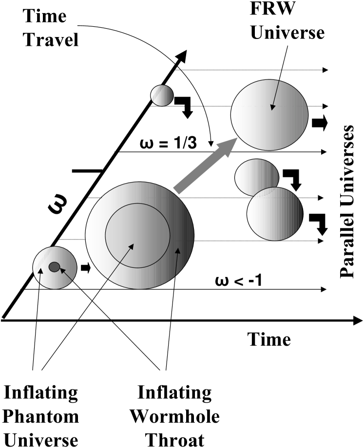
Figure 2: Pictorial representation of the smooth exit from the primordial inflationary process driven by phantom energy. It is based on the time-travelling of a whole, sufficiently inflated, universe from the phantom-energy dominated regime to the usual radiation-dominated regime. Such a nonchronal process is chosen by anthropic arguments over all other possible cosmological final configurations allowed by the many-worlds interpretation of the quantum mechanics of the early universe.

After $t=\bar{t}$, the phantom universe as a whole enters a noncausal phase where it can travel through time in a non-chronal way, back to its origin or toward its future to get, relative to present observers in our universe, into the observable Friedmann cosmology we are familiar with. Among all the presumably infinite number of possible future destinations of the primordial cosmic time travel, which are allowed by the quantum parallel universe picture, the anthropic principle would in this way choose only that future evolution which is governed by the observable Friedmann scenario dominated by radiation with $\omega=1/3$, leaving the remaining potentially evolutionary cosmological solutions as aborted possibilities, relative to present human-being civilization (Fig. 2).

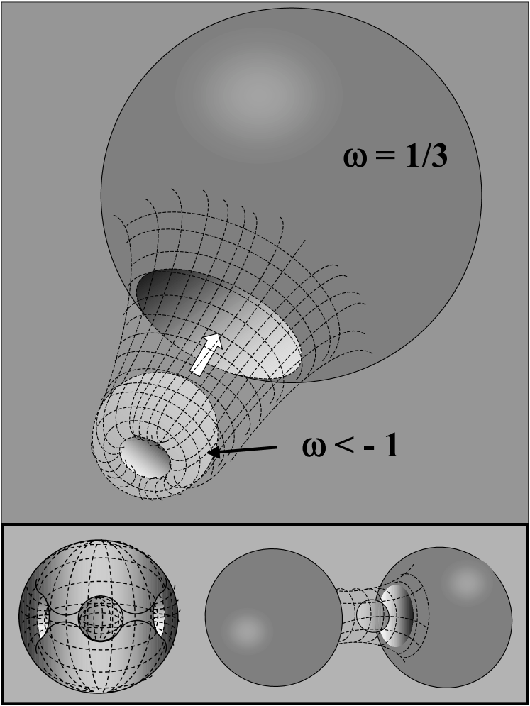
Figure 3: Pictorial representation of the time travel process by which a phantom universe with $\omega<-1$ gets in a universe with $\omega=1/3$ in its future. That process is carried out by using the topology represented in upper part of this figure by which an inflated wormhole whose size has exceeded the radius of the phantom universe itself inserts one of its mouths in the phantom universe while its other mouth is inserted in the host universe. In the inset at the bottom of the figure we also show the other two possible topologies that the larger wormhole throat and the phantom universe may adopt. On the left it is the topology involving just the phantom universe and the wormhole, and on the right we show the most complicated topology where, besides the phantom universe and the wormhole, there are two extra universes in which the two wormhole mouths are respectively inserted.

Since the general $\omega$-dependent expressions for radiation temperature and energy density are respectively given by [11] $\Theta\propto(1+\omega)a^{-3\omega}$ and $\rho\propto[\Theta/(1+\omega)]^{(1+\omega)/\omega}$, and hence the temperature of the phantom universe is negative and therefore hotter than that of the host universe, time travelling from a $\omega<-1$ universe to a $\omega=1/3$ universe (both assumed to be different eigenstates of the same quantum-mechanical cosmic wave equation, see Fig. 3) will naturally follow the natural flow of energy and globally convert a radiation field which was initially characterized by a negative temperature with very large absolute value and a very large energy density, at $\omega<-1$, into a radiation field at positive temperature with quite smaller absolute value and quite smaller energy density, at $\omega=1/3$ (because cosmological effects dictated by the eigenvalue of $\omega$ will prevail over microscopic, local effects globally). At the same time that such a cosmological conversion takes place, however, the phantom stuff should locally interact with the stuff of the host Friedmann universe, as these stuffs should initially preserve their microscopic and thermodynamic original properties locally. In fact, within a given small volume $\delta V$ filled with phantom energy the internal energy, $\delta U=(1+\omega)\rho\delta V$, is definite negative and its absolute value quite larger than that for the positive internal energy of the radiation initially in the host universe, within the same volume $\delta V$. As a result from that initial local interaction, all of the energy initially present in the host universe was annihilated, while almost all phantom radiation remained practically unaffected microscopically, but would globally behave like though if cosmologically it was the $\omega=1/3$-radiation initially contained in the Friedmann universe after having undergone an inflationary period, in spite of the fact that a universe with $\omega=1/3$ by itself could never undergo primordial inflation or reheating without including an extra inflaton field, which we do not assume to exist. Thus, for a current observer, the transferred phantom radiation left after microscopic interaction would just be the customary microwave background radiation characterized by a parameter $\omega=1/3$.

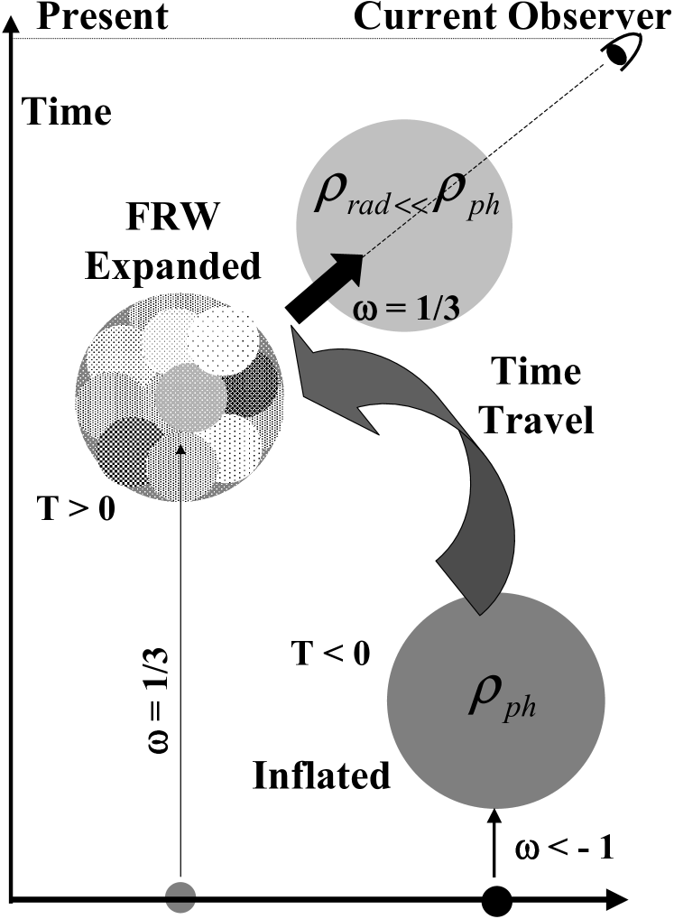
Figure 4: Uniformity is transferred from the inflated phantom universe to our universe when the former universe is absorbed by the latter universe after the time travel. Before the moment of time travelling, our universe was completely causally disconnected with respect to current observers. As the phantom universe was hotter than ours, when they came in contact all the uniformly distributed energy in it was transferred into our universe, annihilating all its inhomogeneities and thereby disappearing.

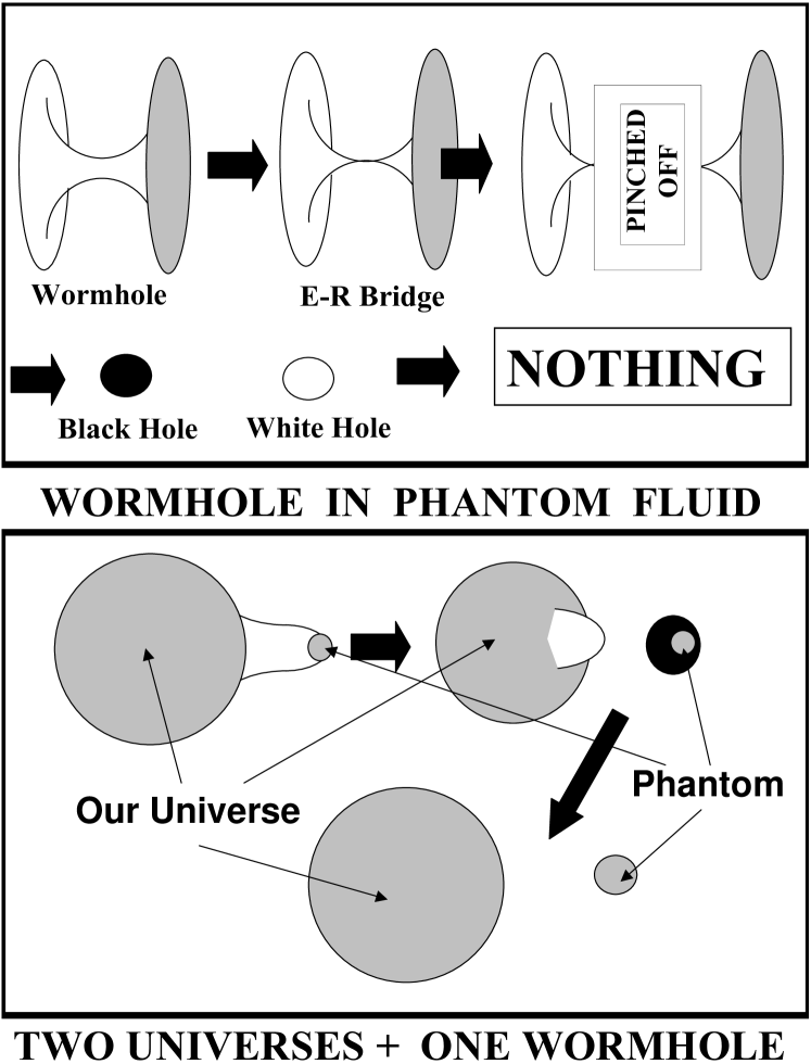
Figure 5: Upper part: After time $t=\tilde{t}$ a single wormhole is immediately converted into a Einstein-Rosen bridge whose throat rapidly pinches off, leaving a black hole plus a white hole. These holes will then fade rapidly off by continuing accreting phantom energy. Lower part: The same regime for the case of a wormhole connecting a phantom universe with another distinct universe like ours. In this case, each of these two universes is first enclosed in a giant black hole or white hole which are mutually disconnected. Then, the holes fade rapidly off and finally the two disconnected universes are left as the sole result of the whole process.

It follows that, relative to current observers, besides transferring a subdominant proportion of matter, the overall neat observable effect induced on the Friedmann universe when a whole phantom universe is transferred by a time travel act into it would in practice be converting the relative-to-current-observers causal disconnectedness owing to the inflationless universe into full causal connectedness of all of its components, relative to such observers, so solving any uniformity and horizon problems (Fig. 4). In this way, we would no longer expect ourselves to be made just of the matter and positive energy created at our own universe’s big bang, but rather out of a mixture of such components with the matter and phantom energy created at the origin of a universe other than ours. It is worth remarking that for the considered time travel to take place it must be performed before the wormhole throat radius becomes infinity (that is along the time interval $\Delta_{nonchronal}$ in Fig. 1), since otherwise the wormhole is converted into a Einstein-Rosen bridge whose throat would immediately pinches off, leaving a pair black-white holes which accrete phantom energy and rapidly vanish [3] (see Fig. 5).

We shall finally notice that, relative to a ”quantum” observer (i.e. an observer able to simultaneously observe all the eigenuniverses), the whole process we have just discussed violates the second law of thermodynamics. In fact, if we disregard the matter contents of the universes, then the entropy of each of these universes is a given universal constant $\sigma$ [11], and therefore the total initial entropy would be $n\sigma$, with $n$ the number of eigenuniverses. After the above discussed time travel, the total entropy would decrease down to a value $(n-1)\sigma$. Moreover, a violation of the second law would also take place relative to an observer in our universe due to the increase of coherence induced in the host universe by exchanging its original radiation content for that carried into it by the phantom universe. These violations of the second law can be thought to be the consequence from the fact that any stuff having phantom energy must be regarded as an essentially quantum stuff with no classical analog, where negative temperatures and entropies are commonplace, such as has been seen to occur in entangled-state and nuclear spin systems.

The whole scenario discussed in this paper is quite speculative and will of course pose some problems and difficulties which would deserve thorough consideration. The most important problem refers to density and gravitational wave fluctuations which are originated in the phantom inflationary epoch, and the way these predicted fluctuations compare with the temperature fluctuations currently observed in WMAP CMB [12]. Though we do not intend to perform a complete investigation on such subjects in this paper, a brief discussion appears worth considering. From Eqs. (15), (18) - (20), it can be shown that the slow-climb conditions for our phantom inflation model are

$$\epsilon_{{\rm ph}}=-\frac{\dot{H}}{H^{2}}=\frac{3}{2}(|\omega|-1)<<1,\;\;\;\delta{{\rm ph}}=-\frac{\ddot{\Phi}}{\dot{\Phi}H}=\epsilon_{{\rm ph}}<<1,$$ (19)

where $H=\dot{a}/a$. When conditions (26) are satisfied the scale factor will approximately evolve with time in an exponential, de Sitter like way, while the parameter $\omega<-1$ must take on values which are very close to -1. Metric perturbations can then be studied following e.g. the procedure in Ref. [2]. Thus, in the longitudinal gauge and absence of anisotropic stresses, the scalar metric perturbations can be expressed in terms of a perturbed metric as a function of both the Bardeen potential, $V_{B}$, and the conformal time $\eta=\int dt/a(t)$, with $a(\eta)=\left[-(|\omega|-1)\eta/2\right]^{-2/[2(|\omega|-1)]}$. As expressed in terms of the Bardeen potential as well, the curvature perturbation on uniform comoving hypersurface is then given by

$$\varsigma=V_{B}+\frac{(3|\omega|-1)\eta V_{B}^{\prime}-2V_{B}}{3(|\omega|-1)},$$ (20)

where ${}^{\prime}=d/d\eta$. It follows that the differential equation of motion for the perturbation $\varsigma$ can be written as

$$\vartheta_{k}^{\prime\prime}+\left(k^{2}-\frac{2(1+3|\omega|)}{(3|\omega|-1)^{2}\eta^{2}}\right)\vartheta_{k}=0,$$ (21)

where $\vartheta=a^{2}\Phi^{\prime}\varsigma/a^{\prime}=z\varsigma$, with $z=\sqrt{\rho_{0}(|\omega|-1)}\left(-(3|\omega|-1)\eta/2\right)^{-2/(3|\omega|-1)}$. Eq. (28) admits an exact analytical solution in terms of the Bessel function $B$ [13]:

$$\vartheta_{k}=\eta^{1/2}B_{\frac{3(1+|\omega|)}{2(3|\omega|-1)}}\left(k\eta\right)\simeq\eta^{1/2}B_{\frac{3}{2}+\epsilon_{{\rm ph}}}\left(k\eta\right),$$ (22)

the last approximate equation being valid if the slow-climb conditions are satisfied. The inclusion of suitable initial conditions will choose the precise Bessel function we should use. The amplitude associated with this perturbation can then be given by [2]

$$A_{s}=\frac{2}{3(|\omega|-1)(T^{\prime})^{2}_{k=aH}},$$ (23)

while the spectral index becomes $n_{s}=\frac{3}{2}\left(\frac{5|\omega|-3}{3|\omega|-1}\right)$. The amplitude for tensor perturbation can be analogously derived. It reads

$$A_{t}=\left(\frac{1}{T^{\prime}}\right)^{2}_{k=aH},$$ (24)

with a spectral index $n_{t}\simeq-3(|\omega|-1)$.

The ratio $A_{t}/A_{s}=3(|\omega|-1)/2\simeq\epsilon_{{\rm ph}}$ should now be compared with the tensor/scalar ratio of CMB quadrupole contributions, $r\sim\epsilon_{{\rm ph}}$, to low order. Our phantom scenario with $\epsilon_{{\rm ph}}=\delta_{{\rm ph}}$ and exponential potential differs from other phantom inflation models [2], and a thorough join comparation of all of these models with the usual scalar field inflationary scenarios on the $r-n_{s}$ plane is left for a future publication. Actually, just like it happens with scalar field models for inflation, the phantom inflation scenarios could only be taken seriously if they succeeded in predicting the types of temperature fluctuations discovered from the WMAP CMB data.

Acknowledgements The author thanks Carmen L. Sigüenza for useful information exchange and comments. This work was supported by DGICYT under Research Project No. BMF2002-03758.

References

1

J.S. Alcaniz, Phys. Rev. D69, 083521 (2004) , and references therein.

2

Y-S. Piao and Y.-Z. Zhang, astro-ph/0401231

3

P.F. González-Díaz, astro-ph/0404045, Phys. Rev. Lett. (in press, 2004)

4

Visser, Lorentzian Wormholes (AIP Press, WoodburyNew York, USA, 1995); S. Nojiri, O. Obregon, S.D. Odintsov and K.E. Osetrin, Phys. Lett. B449, 173 (1999).

5

P.F. González-Díaz, Phys. Rev. D68, 084016 (2003).

6

R.R. Caldwell, Phys. Lett. B545, 23 (2002); R.R. Caldwell, M. Kamionkowski and N.N. Weinberg, Phys. Rev. Lett. 91, 071301 (2003); P.F. González-Díaz, Phys. Rev. D68, 021303 (2003); J.D. Barrow, Class. Quant. Grav. 21, L79 (2004); M. Bouhmadi and J.A. Jiménez- Madrid, astro-ph/0404540 .

7

J.B. Hartle and S.W. Hawking, Phys. Rev. D28, 2960 (1983); S.W. Hawking, Phys. Rev. D32, 2489 (1985); S.W. Hawking, Quantum Cosmology, in: Relativity Groups and Topology, Les Houches Lectures, edited by B. DeWitt and R. Stora (North-Holland, 1984).

8

See the contributions in the book The Many-Worlds Interpretation of Quantum Mechanics, edited by B.SDeWitt and N. Graham (Princeton University Press, Princeton, New Jersey, USA, 1973).

9

J.D. Barrow and F.J. Tipler, The Anthropic Cosmological Principle (Clarendon Press, Oxford, UK, 1986).

10

P.F. González-Díaz, Phys. Rev. D69, 063522 (2004).

11

P.F. González-Díaz and C.L. Sigüenza, Phys. Lett. B589, 78 (2004).

12

W.K. Kinney, E.W. Kolb, A. Melchiorri and A. Riotto, Phys. Rev. D69, 103516 (2004)

13

M. Abramowitz and I.A. Stegun, Handbook of Mathematical Functions (Dover, New York, USA, 1965).