UOA/NPPS-07/04

1 Introduction

Model building constructions (MBC’s) in the context of string theory have by far been explored both into the context of open string and heterotic string compactifications where a number of semirealistic have been explored and analyzed [1]. In the absence of a dynamical principle for selecting a particular string vacuum and simultaneously fix all moduli, the standard lore is to systematically analyze on phenomenological grounds the different string compactifications and trying to derive a miminal supersymmetric vaccum that may contain the Minimal Supersymmetric Standard Model (MSSM) if possible in the presence of a few exotics. Moreover, over the last few years, MBC’s coming from intersecting branes (IB’s) [2]-[42] have received a lot of attention as it become possible to construct - for the first time in string theory - non-supersymmetric (non-susy) four dimensional (4D) vacua with only the SM at low energy using intersecting D6-branes [10],[11], [12], [14] from 4D toroidal orientifolds of type IIA. For other attempts to derive the SM from string theory see [15]. In this regard, vacua based on non-SUSY Pati-Salam GUT constructions (with a stable proton), which break to the SM at low energy, giving masses to all exotics, have been also constructed and analyzed [13]. All the above models have vanishing RR tadpoles and uncancelled NS-NS tadpoles (coming from the closed string sector), the latter acting as an effective cosmological constant [6]. On phenomenological grounds the string scale may be at the TeV; however as the D6-branes wrap the whole of internal space and there are no dimensions transverse to all branes, the presence of a TeV scale cannot be explained according to the AADD mechanism [18].
Nevertheless, we note that intersecting brane worlds accommodate nicely the AADD [18] solution to the gauge hierarchy problem by providing us with the only known string realization in these backgrounds. Non-supersymmetric semirealistic GUTS in $Z_{3}$ orientifolds of interesting branes have been also analyzed for SU(5) [6]. Flipped SU(5) GUTS were constructed [7] and the existence of appropriate Higgses necessary for the correct electroweak breaking to the SM at low energy and the doublet-triplet splitting mechanism has been shown [22]. The SU(5)/flipped SU(5) models are missing perturbatively the up/down quark couplings

Moreover, the construction of vacua which have only the MSSM at low energies, has been also studied using either N=1 supersymmetric models or N=0 models that localize in part of their spectrum the MSSM. In the latter case, the MSSM is localized as part of the non-supersymmetric open string spectrum where particles respect different N=1 supersymmetries [24, 25] or where each particle of the MSSM preserves the same N=1 susy and the rest of the spectrum a different N=1 susy[26, 20] In the former case, N=1 semirealistic supersymmetric vacua based on intersecting D6-branes has also been explored in four dimensional orientifolds of type IIA on ${\bf T^{6}/Z_{2}\times Z_{2}}$ [9], ${\bf T^{6}/Z_{4}}$[31], ${\bf T^{6}/Z_{2}\times Z_{4}}$ [32], and ${\bf T^{6}/Z_{6}}$ [33], Z12-II [34] and also N=1 GUT constructions have been analyzed [9]. The main characteristics of these models is that not all complex structure moduli are fixed and part of their spectrum includes those of the N=1 SM (MSSM) in addition to extra massless chiral exotics [9], [33] or massless non-chiral exotics [31] [We also note that there are model building attempts from orientifolds of Gepner constructions where also the N=1 SM, with three pairs of $H_{u}$, $H_{d}$ MSSM Higgs multiplets, was found but in the presence of extra massless non-chiral exotics [43].] While supersymmetric models have no gauge hierarchy problem and are stable vacua as they do not have RR $\&$ NSNS tadpoles, we we will focus our attention to the MBC of non-supersymmetric models on 4D $Z3\times Z3$ IIA orientifolds [27] for several reasons. First of all, the satisfaction RR tadpoles and Green-Schwarz anomaly cancellation mechanism cancels all gauge anomalies . Flavour changing neutral currents that could be a problem in low scale models $\sim 10^{2}$ TeV [38] may be avoided as the scale of the models we study is at least $10^{13}$ GeV and higher. There is no sign of any supersymmetry after the present 7 TeV run of LHC. At present there is no hint from squarks and gluinos below 1 TeV from their R-parity channels in the MSSM. Unification of of the three gauge couplings constants works fine in the MSSM and does not work in the SM. In the context of intersecting branes [52], two of the gauge couplings unify, in a general N=1 supersymmetric model. Non-supersymmetric unification that we will study in this paper, is an open question. Complex moduli which can generate tadpoles are absent and the corresponding tadpoles vanish in the present models. Thus the effect of the orbifold symmetries in the present models that fix complex structure moduli, is equivalent to the effects we achieve, by turning on arbitrary fluxes on three-cycles invariant under the discrete symmetry [60]. Alternatively, one is using IIB to fix moduli [61]. Only the dilaton has a only non-vanishing tadpole, which could cause an instability. However, this problem is unsolved and it is possible that the vacua re-adjust themselves so that the true vacuum is reached when all orders are taken into account in perturbation theory [29].

The purpose of this paper is to discuss the appearance of N=0 supersymmetric models that break to only the SM either without any exotics being present or with a minimal number of chiral massive exotics [three (3) vector pairs]. These models are based on four dimensional type IIA orientifolds on ${\bf T^{6}/{\bf Z_{3}\times Z_{3}}}$ with D6-branes intersecting at angles [27]. In the N=0 intersecting D6-brane models presented in this work there are several interesting features :
a) Models which achieve the successful GUT result for the Weinberg angle, $sin^{2}\theta=3/8$ are presented. b) at the level of 3-stacks, we find models which break to only the SM at low energy. We also find non-susy models - at 3- and 5-stacks - with the chiral spectrum of the N=1 SM (with $\nu_{R}$’s) in the presence of three pairs of MSSM Higgsinos $H_{u}$, $H_{d}$ in addition to massive non-chiral exotics which again break to the SM at low energies. A comment is in order. In this work when we will speak about the SM, we will keep in mind that in all models there is no mass term for the up-quarks [The same effect persists in the models of [6, 67]]. Instantons oud be recalled to generate the masses [48, 49].
Recently the split supersymmetry scenario (SS) was proposed [50]. In this respect we propose intersecting D-brane models that provide evidence for a natural realization of the SS scenario in intersecting D-brane models as they satisfy most of the relevant criteria required by the SS existence.

The outline of the paper is as follows. In chapter 2, we will present the key features of the ${\bf T^{6}/{\bf Z_{3}\times Z_{3}}}$ constructions, including the gauge group structure and spectrum rules. The details of the construction for the AAA, AAB, BBB lattice have been presented in a companion paper [27]. In chapter 3, we discuss N=0 three generation (3G) non-supersymmetric SM’s with the fermion spectrum of the N=1 SM and extra non-chiral massive SU(3) triplet exotics. Higgsinos get massive and the models break to the SM at low energy. In chapter 4 we also discuss the deformation of these N=0 3G models to other N=0 3G models which have only the SM the low energy without any exotics being present. In chapter 5, we examine whether or not it is possible to construct N=0 models by using 4-stacks of D6’s. In chapter 6 we present more possibilities for constructing N=0 3G models by using five stacks of intersecting D6-branes. Here it is also possible to construct N=0 vacua with only the SM at low energy and extra non-chiral massive exotics. In chapter 7 we construct N=0 eight stack models with the N=1 SM fermionic spectrum made from N=1 SUSY preserving D6-branes. In chapter 8, we present the spectrum rules for the $Z3\times Z3$ on the ABB lattice. In chapter 9 we present arguments supporting the relevance of intersecting D-brane constructions to some new ideas related to the existence of split supersymmetry in nature and also discuss models with $sin^{2}\theta=3/8$ at the string scale that satisfy most of the conditions required for the split susy scenario. Chapter 10, examines the unification of gauge couplings for the split susy models of Chapter 9 describing the SM unification from non-susy intersecting branes. Chapter 11 contains our conclusions.

2 Spectrum on $T^{6}/Z_{3}\times Z_{3}$ orientifolds, RR tadpoles $\&$ anomaly cancellation

Our orientifold constructions originate from IIA theory compactified on the ${\bf T^{6}/(Z_{3}\times Z_{3})}$ orbifold, where the latter symmetry is generated by the twist generators (where $\alpha=e^{\frac{2\pi i}{3}}$) $\theta:(z_{1},z_{2},z_{3})\rightarrow(\alpha z_{1},\alpha^{-1}z_{2},z_{3})$, $\omega:(z_{1},z_{2},z_{3})\rightarrow(z_{1},\alpha z_{2},\alpha^{-1}z_{3})$, where $\theta$, $\omega$ get associated to the twists $\upsilon=\frac{1}{3}(1,-1,0)$, $u=\frac{1}{3}(0,1,-1)$. Here, $z^{i}=x^{i+3}+ix^{i+5}$, $i=1,2,3$ are the complex coordinates on the $T^{6}$, which we consider as being factorizable for simplicity, e.g. $T^{6}=T^{2}\otimes T^{2}\otimes T^{2}$. In addition, to the orbifold action the IIA theory is modded out by the orientifold action $\Omega R$ that combines the worldsheet parity $\Omega$ and the antiholomorphic operation $R:z^{i}\rightarrow{\bar{z}}^{i}$. Because the orbifold action has to act crystallographically on the lattice the complex structure on all three $T^{2}$ tori is fixed to be $U^{I}_{A}=1/2-i\sqrt{3}/2$. The lattice vectors are defined as $e_{1}=(1,0)$,  $e_{2}=(-1/2,\sqrt{3}/2)$ and the $\Omega R$ action is along the horizontal directions across the six-torus. The model contains nine kinds of orientifold planes, that get associated to the orbit $\cal O$ consisting of the actions of $\Omega R$, $\Omega R\theta$, $\Omega R\omega$, $\Omega R\theta^{2}$, $\Omega R\omega^{2}$, $\Omega R\theta\omega$, $\Omega R\theta^{2}\omega$, $\Omega R\theta\omega^{2}$, $\Omega R\theta^{2}\omega^{2}$. We will be interested on the open string spectrum and not discuss the closed string spectrum that contains gravitational multiplets and orbifold moduli. In order to cancel the RR crosscap tadpoles introduced by the introduction of the orientifold planes we introduce N D6_a-branes wrapped along three-cycles that are taken to be products of one-cycles along the three two-tori of the factorizable $T^{6}$. A D6-brane $a$ - associated with the equivalence class of wrappings $(n^{I},m^{I})$, $I=1,2,3$, - is mapped under the orbifold and orientifold action to its images

$$a\leftrightarrow\left(\begin{array}[]{c}n_{a}^{1},m_{a}^{1}\\ n_{a}^{2},\ m_{a}^{2}\\ n_{a}^{3},\ m_{a}^{3}\end{array}\right),\ \theta a\rightarrow\left(\begin{array}[]{c}-m_{a}^{1},\ (n-m)_{a}^{1}\\ (m-n)_{a}^{2},\ -n_{a}^{2}\\ n_{a}^{3},\ m_{a}^{3}\end{array}\right),\ \ \Omega Ra\rightarrow\left(\begin{array}[]{c}(n-m)_{a}^{1},\ -m_{a}^{1}\\ (n-m)_{a}^{2},\ -m_{a}^{2}\\ (n-m)_{a}^{3},\ -m_{a}^{3}\end{array}\right)\ .$$ (2.10)

In $\Omega R$ orientifolds the twisted disk tadpoles vanish [39]. The $Z_{3}\times Z_{3}$ orientifold models are subject to the cancellation of untwisted RR tadpole conditions [27] given by

$$\sum_{a}N_{a}Z_{a}=4,$$ (2.11)

where

$$Z_{a}=2m^{1}_{a}m^{2}_{a}m^{3}_{a}+2n^{1}_{a}n^{2}_{a}n^{3}_{a}-n_{a}^{1}n_{a}^{2}m_{a}^{3}-n_{a}^{1}m_{a}^{2}n_{a}^{3}-m_{a}^{1}n_{a}^{2}n_{a}^{3}-m_{a}^{1}m_{a}^{2}n_{a}^{3}-m_{a}^{1}n_{a}^{2}m_{a}^{3}-n_{a}^{1}m_{a}^{2}m_{a}^{3}$$ (2.12)

The gauge group U($N_{a}$) supported by $N_{a}$ coincident D6_a-branes comes from the $a({\tilde{a}})$ sector, the sector made from open strings stretched between the $a$-brane and its images under the orbifold action. In addition, we get three adjoint N=1 chiral multiplets. In the $a({\cal O}b)$ sector - strings stretched between the brane $a$ and the orbit images of brane $b$ - will localize $I_{ab}$ fermions in the bifundamental $(N_{a},{\bar{N}}_{b})$ where

$$I_{ab}=3(Z_{a}Y_{b}-Z_{b}Y_{a}),$$ (2.13)

and $(Z,Y)$ are the effective wrapping numbers with $Y_{a}$ given by

$$Y_{a}=m^{1}_{a}m^{2}_{a}m^{3}_{a}+n^{1}_{a}n^{2}_{a}n^{3}_{a}-n^{1}_{a}n^{2}_{a}m^{3}_{a}-n^{1}_{a}m^{2}_{a}n^{3}_{a}-m^{1}_{a}n^{2}_{a}n^{3}_{a}$$ (2.14)

The sign of $I_{ab}$ denotes the chirality of the associated fermion, where we choose positive intersection numbers for left handed fermions. In the sector ${ab^{\prime}}$ - strings stretching between the brane $a$ and the orbit images of brane $b$, there are $I_{ab^{\prime}}$ chiral fermions in the bifundamental $(N_{a},N_{b})$, with

$$I_{ab^{\prime}}=3(Z_{a}Z_{b}-Z_{a}Y_{b}-Z_{b}Y_{a}),$$ (2.15)

The theories also accommodate the following numbers of chiral fermions in symmetric (S) and antisymmetric (A) representations of $U(N_{a})$ from open strings stretching between the brane $a$ and its orbit images $({\cal O}a)$,

$$(A_{a})=3(Z_{a}-2Y_{a}),$$ (2.16)

$$(A_{a}+S_{a})=\frac{3}{2}(Z_{a}-2Y_{a})(Z_{a}-1)$$ (2.17)

Finally, from open strings stretched between the brane $a$ and its orbifold images we get non-chiral massless fermions in the adjoint representation,

$$(Adj)_{L}:\prod_{i=1}^{3}(L^{I}_{[a]})^{2}\ ,$$ (2.18)

where

$$L^{I}_{[a]}=\sqrt{(m_{a}^{I})^{2}+(n_{a}^{I})^{2}-(m_{a}^{I})(n_{a}^{I})}$$ (2.19)

Adjoint massless matter, including fermions and gauginos that are massless at tree level are expected to receive string scale masses from loops once supersymmetry is broken , leaving only the gauge bosons massless, and we will not discuss it further. In the low energy theory, cubic gauge anomalies automatically cancel, due to the RR tadpole conditions (2.11). Mixed U(1)-gauge anomalies also cancel due to the existence of a generalized Green-Schwarz (GS) mechanism (see [27] for further details) that makes massive only one U(1) gauge field given by

$$\sum_{a}N_{a}(Z_{a}-2Y_{a})F_{a}$$ (2.20)

The minimal choice of obtaining an extension of the Standard model (SM) is obtained using three stacks of D6-branes. The spectrum of open strings stretching between intersecting D6-branes is calculated by the use of rules (2.4 - 2.8). To establish notation we will denote the type of sypersymmetries preserved in the closed string sector by the choices of vectors $r_{0}=\pm(1/2)(+-+-)$, $r_{1}=\pm(1/2)(++--)$, $r_{2}=\pm(1/2)(-++-)$, $r_{3}=\pm(1/2)(----)$. Supersymmetry may be preserved by a system of branes if each stack of D6-branes is related to the $O6$-planes by a rotation in $SU(3)$, that is the angles ${\tilde{\theta}}_{i}$ of the D6-branes with respect to the horizontal direction in the i-th two-torus obeys the condition ${\tilde{\theta}}_{1}+{\tilde{\theta}}_{2}+{\tilde{\theta}}_{3}=0$. The supersymmetry of the models that is preserved by any pair of branes is determined by the choice of the orbifold and orientifold action. To examine whether N=0 or N=1 susy models are allowed we have to examine the brane wrappings $(n,m)$. Our current search finds no N=1 supersymmetric models but only N=0 ones, in chapter 8, made from different preserving supersymmetries.

3 The N=0 MSSM

Next, we obtain non-supersymmetric models which localize the fermion spectrum of the intersecting brane N=1 MSSM in addition to a couple of massive - non-chiral - exotics, which subsequently break to only the SM at low energy with the use of the GS mechanism described in the previous section.

3.1 N=0 SM’s at low energy with the N=1 MSSM fermion spectrum at $M_{s}$

The minimal choice of obtaining the SM gauge group and chiral spectrum is to start from a three stack $U(3)_{a}\times U(2)_{b}\times U(1)_{c}$ D6-brane construction at the string scale. The choice of wrapping numbers

$$(Z_{a},Y_{a})=\left(\begin{array}[]{cc}1,&0\\ \end{array}\right),\ (Z_{b},Y_{b})=\left(\begin{array}[]{cc}1,&1\\ \end{array}\right),\ (Z_{c},Y_{c})=\left(\begin{array}[]{cc}-1,&1\\ \end{array}\right)$$ (3.1)

satisfies the RR tadpoles and corresponds to the spectrum seen in table (1).

Model structure	${\bf Particles\hskip 28.45274pt}$	${\bf(SU(3)\times SU(2))_{(Q_{a},Q_{b},Q_{c})}}\hskip 28.45274pt$	${\bf U(1)^{Y}}$
$MSSM\ QUIVER$	$\hskip 56.9055pt\{Q_{L}\}\hskip 28.45274pt$	$3({3},{2})_{(1,\ -1,\ 0)}\hskip 28.45274pt$	$1/6$
	$\hskip 56.9055pt\{u_{L}^{c}\}\hskip 28.45274pt$	$\#\raisebox{-3.5pt}{\hbox{\rule{0.4pt}{6.5pt}\hskip-0.4pt\rule{6.5pt}{0.4pt}\hskip-6.5pt\rule[6.5pt]{6.5pt}{0.4pt}}\rule[6.5pt]{0.4pt}{0.4pt}\hskip-0.4pt\rule{0.4pt}{6.5pt}}\hskip-6.9pt\raisebox{3.0pt}{\hbox{\rule{0.4pt}{6.5pt}\hskip-0.4pt\rule{6.5pt}{0.4pt}\hskip-6.5pt\rule[6.5pt]{6.5pt}{0.4pt}}\rule[6.5pt]{0.4pt}{0.4pt}\hskip-0.4pt\rule{0.4pt}{6.5pt}}\ =3(3,1)_{(2,\ 0,\ 0)}\hskip 28.45274pt$	$-2/3$
	$\hskip 56.9055pt\{d_{L}^{c}\}\hskip 28.45274pt$	$3(3,1)_{(-1,\ 0,\ -1)}\hskip 28.45274pt$	$1/3$
	$\hskip 56.9055pt\{L\ +\ H_{d}\}\hskip 28.45274pt$	$6(1,2)_{(0,\ 1,\ -1)}\hskip 28.45274pt$	$-1/2$
	$\hskip 56.9055pt\{H_{u}\}\hskip 28.45274pt$	$3(1,{\bar{2}})_{(0,\ -1,\ -1)}\hskip 28.45274pt$	$1/2$
	$\hskip 56.9055pt\{e_{L}^{+}\}\hskip 28.45274pt$	$\#\bar{\raisebox{-3.5pt}{\hbox{\rule{0.4pt}{6.5pt}\hskip-0.4pt\rule{6.5pt}{0.4pt}\hskip-6.5pt\rule[6.5pt]{6.5pt}{0.4pt}}\rule[6.5pt]{0.4pt}{0.4pt}\hskip-0.4pt\rule{0.4pt}{6.5pt}}\hskip-6.9pt\raisebox{3.0pt}{\hbox{\rule{0.4pt}{6.5pt}\hskip-0.4pt\rule{6.5pt}{0.4pt}\hskip-6.5pt\rule[6.5pt]{6.5pt}{0.4pt}}\rule[6.5pt]{0.4pt}{0.4pt}\hskip-0.4pt\rule{0.4pt}{6.5pt}}}\ =3(1,1)_{(0,\ -2,\ 0)}\hskip 28.45274pt$	$1$
	$\hskip 56.9055pt\{{N_{R}}\}\hskip 28.45274pt$	$\#\raisebox{-0.5pt}{\hbox{\rule{0.4pt}{6.5pt}\hskip-0.4pt\rule{6.5pt}{0.4pt}\hskip-6.5pt\rule[6.5pt]{6.5pt}{0.4pt}}\rule[6.5pt]{0.4pt}{0.4pt}\hskip-0.4pt\rule{0.4pt}{6.5pt}}\hskip-0.4pt\raisebox{-0.5pt}{\hbox{\rule{0.4pt}{6.5pt}\hskip-0.4pt\rule{6.5pt}{0.4pt}\hskip-6.5pt\rule[6.5pt]{6.5pt}{0.4pt}}\rule[6.5pt]{0.4pt}{0.4pt}\hskip-0.4pt\rule{0.4pt}{6.5pt}}\ =9(1,1)_{({0},\ {0},\ {2})}\hskip 28.45274pt$	$0$
Extra  Matter	$\hskip 56.9055pt\{C_{1}\}\hskip 28.45274pt$	$3(3,\ 1)_{(1,\ 0,\ -1)}\hskip 28.45274pt$	$1/3$
	$\hskip 85.35826pt\{C_{2}\}\hskip 56.9055pt$	$3({\bar{3}},1)_{(-1,\ 0,\ -1)}\hskip 28.45274pt$	$-1/3$

Table 1: A three generation non-supersymmetric model with the fermion content of N=1 MSSM on top of the table, in addition to $N_{R}$’s and three pairs of $H_{u}$, $H_{d}$ Higgsinos. This model predicts nine $N_{R}$’s that could be written as a linear combination of three $N_{R}$’s. Note that this model mimics models coming from gauge mediation scenarios.

We recognize in table (1), the chiral spectrum of the N=1 MSSM with three generations of right handed neutrinos ($N_{R}$) and three pairs of massless ‘Higgsinos’ . Also one U(1) gauge field becomes massive through its BF couplings, namely

$$U(1)^{massive}=3F_{a}-2F_{b}-3F_{c}$$ (3.2)

There hypercharge obeys the massleness condition

$$U(1)^{massive}\cdot U(1)^{massless}\ =0$$ (3.3)

thus surviving massless the GS mechanism (2.20). The hypercharge reads:

$$Y\ =\ U(1)^{Y}\ =\ -(1/3)F_{a}-(1/2)F_{b}$$ (3.4)

The second U(1)’s that survive massless the (3.3)

$$U(1)^{add}=F_{a}-(2/3)F_{b}+(13/3)F_{c}\ .$$ (3.5)

$U(1)^{add}$ could be broken by a tachyonic singlet excitation charged under $F_{c}$, namely ${\tilde{N}}_{R}$, that plays the role of the ‘superpartner’ of $N_{R}$, thus leaving only the hypercharge $U(1)^{add}$ massless at low energies, below the scale set by $\langle{\tilde{N}}_{R}\rangle$. The following Yukawa couplings for the quarks, leptons and exotics $X_{i}$ are allowed:

$$Y=\lambda_{d}\ Q_{L}d^{c}_{L}{\tilde{H}}_{d}{\tilde{N}}_{R}/M_{s}+\lambda_{u}^{ij}\ L^{j}N_{R}^{i}{\tilde{H}}_{u}\ +\lambda_{E}LE_{R}{\tilde{H}}_{d}{\tilde{N}}_{R}/M_{s}\ +\$$

$$\lambda_{C}C_{1}C_{2}{\tilde{N}}_{R}\ +\lambda_{\mu}H_{u}H_{d}{\tilde{N}}_{R}\ \ i=1,.,9;\ j=1,2$$ (3.6)

The exotic triplets $C_{i}$ form a Dirac mass term which receives a mass of order $M_{s}$ from the vev of ${\tilde{N}}_{R}$. The form of this coupling provide us with the bilinear mixing, that in a N=1 susy theory, would have played the role of a superpotential $\mu$-term. We remind that because the D6-branes wrap along all the $T^{6}$, the string scale is high and close to the Planck scale. Thus the two Higgsinos $H_{u}$, $H_{d}$ receive a Dirac mass term from the last term in (3.6) of order of the string scale, as the natural scale of $\langle N_{R}\rangle=M_{s}$. However, the value for the Higgsinos which can be at $M_{s}$ or lower is set by the values of the Yukawa coupling coefficients $\lambda_{\mu}$. Large exponential suppression of a n-point interaction of Yukawa interactions in the form

$$\lambda_{\mu}\sim e^{-A}$$ (3.7)

is a natural aspect of IBW’s due to their dependence on the worldsheet area $A$, in string units, located between their brane intersections [38, 13]. Hence a light higssino condensate of order of electroweak symmetry breaking $\upsilon=246$ GeV can be obtained, assuming $M_{s}=10^{16}$ GeV, with $A=31$.

The quarks - apart for the u-quark which remain massless as the relevant coupling is excluded from charge conservation - and leptons receive non-zero masses from the Yukawa couplings in the 1st line of (3.6). Thus at low energy we have the SM - with the up quark remaining massless after electroweak symmetry breaking - and nine (9) generations of right handed neutrinos. A comment is in order. As the D6-branes involved wrap on generic angles the spectrum of table (1) is non-supersymmetric. Unfortunately, we were only able to find wrappings that render the models non-supersymmetric.

$Brane$	$\hskip 56.9055pt(n^{1},m^{1})\times(n^{2},m^{2})\times(n^{3},m^{3})$
$\{a\}$	$(1,\ 0)\times(0,\ 1)\times(0,\ -1)$
$\{b\}$	$(0,\ 1)\times(1,\ 0)\times(0,1)$
$\{c\}$	$(0,\ -1)\times(1,\ 1)\times(0,-1)$

Table 2: Wrapping numbers responsible for the generation of the N=0 models of table (1), that have the chiral spectrum of the intersecting brane N=1 MSSM.

One can also check that the choice of effective wrappings

$$(Z_{a},Y_{a})=\left(\begin{array}[]{cc}1,&0\\ \end{array}\right),\ (Z_{b},Y_{b})=\left(\begin{array}[]{cc}1,&1\\ \end{array}\right),\ (Z_{c},Y_{c})=\left(\begin{array}[]{cc}-1,&-2\\ \end{array}\right)$$ (3.8)

gives us also the N=0 chiral MSSM spectrum of table (1) with the same hypercharge assignments.

4 Exactly the SM from three stacks

In this section, we will construct non-supersymmetric models which have exactly the SM gauge group and chiral spectrum and no exotics present. These models will be constructed as a deformation of the models that appeared in table (1). Also in these models there is no mass term allowed from the up-quarks.

4.1 SM deformations of N=0 SM’S from three stacks

$\bullet$ Let us make the choice of wrapping numbers

$$(Z_{a},Y_{a})=\left(\begin{array}[]{cc}1,&0\\ \end{array}\right),\ (Z_{b},Y_{b})=\left(\begin{array}[]{cc}1,&1\\ \end{array}\right),\ (Z_{c},Y_{c})=\left(\begin{array}[]{cc}-1,&-1\\ \end{array}\right)$$ (4.1)

Table 3: A three generation chiral (open string) spectrum accommodating the SM. The required Higgs may come from non-chiral bifundamentals in the $bc$ sector [10, 11, 12] that may trigger brane recombination.

${\bf Matter\hskip 56.9055pt}$	${\bf(SU(3)\times SU(2))_{(Q_{a},Q_{b},Q_{c})}}\hskip 56.9055pt$	${\bf U(1)^{Y}}$
$\hskip 56.9055pt\{Q_{L}\}\hskip 56.9055pt$	$3(3,{2})_{(1,\ -1,\ 0)}\hskip 56.9055pt$	$1/6$
$\hskip 56.9055pt\{u_{L}^{c}\}\hskip 56.9055pt$	${\#\raisebox{-3.5pt}{\hbox{\rule{0.4pt}{6.5pt}\hskip-0.4pt\rule{6.5pt}{0.4pt}\hskip-6.5pt\rule[6.5pt]{6.5pt}{0.4pt}}\rule[6.5pt]{0.4pt}{0.4pt}\hskip-0.4pt\rule{0.4pt}{6.5pt}}\hskip-6.9pt\raisebox{3.0pt}{\hbox{\rule{0.4pt}{6.5pt}\hskip-0.4pt\rule{6.5pt}{0.4pt}\hskip-6.5pt\rule[6.5pt]{6.5pt}{0.4pt}}\rule[6.5pt]{0.4pt}{0.4pt}\hskip-0.4pt\rule{0.4pt}{6.5pt}}}_{a}\ =3({\bar{3}},1)_{(2,\ 0,\ 0)}\hskip 56.9055pt$	$-2/3$
$\hskip 56.9055pt\{d_{L}^{c}\}\hskip 56.9055pt$	$3(3,1)_{(-1,\ 0,\ 1)}\hskip 56.9055pt$	$1/3$
$\hskip 56.9055pt\{L\}\hskip 56.9055pt$	$3(1,2)_{(0,\ 1,\ 1)}\hskip 56.9055pt$	$-1/2$
$\hskip 56.9055pt\{e_{L}^{+}\}\hskip 56.9055pt$	${\#\bar{\raisebox{-3.5pt}{\hbox{\rule{0.4pt}{6.5pt}\hskip-0.4pt\rule{6.5pt}{0.4pt}\hskip-6.5pt\rule[6.5pt]{6.5pt}{0.4pt}}\rule[6.5pt]{0.4pt}{0.4pt}\hskip-0.4pt\rule{0.4pt}{6.5pt}}\hskip-6.9pt\raisebox{3.0pt}{\hbox{\rule{0.4pt}{6.5pt}\hskip-0.4pt\rule{6.5pt}{0.4pt}\hskip-6.5pt\rule[6.5pt]{6.5pt}{0.4pt}}\rule[6.5pt]{0.4pt}{0.4pt}\hskip-0.4pt\rule{0.4pt}{6.5pt}}}}_{b}=3(1,1)_{(0,\ -2,\ 0)}\hskip 56.9055pt$	$1$
$\hskip 56.9055pt\{N_{R}\}\hskip 56.9055pt$	${\#\bar{\raisebox{-0.5pt}{\hbox{\rule{0.4pt}{6.5pt}\hskip-0.4pt\rule{6.5pt}{0.4pt}\hskip-6.5pt\rule[6.5pt]{6.5pt}{0.4pt}}\rule[6.5pt]{0.4pt}{0.4pt}\hskip-0.4pt\rule{0.4pt}{6.5pt}}\hskip-0.4pt\raisebox{-0.5pt}{\hbox{\rule{0.4pt}{6.5pt}\hskip-0.4pt\rule{6.5pt}{0.4pt}\hskip-6.5pt\rule[6.5pt]{6.5pt}{0.4pt}}\rule[6.5pt]{0.4pt}{0.4pt}\hskip-0.4pt\rule{0.4pt}{6.5pt}}}}_{c}=3(1,1)_{(0,\ 0,\ -2)}\hskip 56.9055pt$	$0$

This choice satisfies the RR tadpoles and corresponds to the spectrum seen in table (3). The intersection numbers are

$$I_{ab}=3, (A)_{a}=3, I_{bc^{\star}}=3,$$

$$(A)_{b}=-3, I_{ac}=-3, (A+S)_{c}=-3\ .$$ (4.2)

From (2.20) there is one anomalous U(1) which becomes massive

$$U(1)^{massive}=3F_{a}-2F_{b}+F_{c}$$ (4.3)

and two anomaly free U(1)’s that correspond to the hypercharge and an extra U(1)

$$U(1)^{Y}=-\frac{1}{3}F_{a}-\frac{1}{2}F_{b},\ \ \ U(1)^{ex}=-3F_{a}+2F_{b}+13F_{c}$$ (4.4)

We recognize in table (3) exactly the chiral spectrum of the SM as at this point the spectrum for generic angles is non-supersymmetric. Exactly the same quiver - but with opposite U(1) charges - non-supersymmetric chiral spectrum construction was found in [6] from intersecting D6-branes in $Z_{3}$ orientifolds. In [6] and in the present models the breaking of the extra U(1) surviving massless the Green-Schwarz mechanism proceeds via tachyonic excitations in the sector accommodating the right handed neutrino. Choices of wrappings satisfying the constraints (4.1) can be seen in table (4). Other choices of wrappings solving the RR tadpole conditions may be seen in table (5). Baryon (and lepton) number is not conserved but as the string scale in these models is naturally close to Planck scale we do expect a natural enhancement of gauge mediated proton decay modes and thus proton stability is guaranteed. The exchange of wrappings

$$(Z_{a},Y_{a})\leftrightarrow(Z_{b},Y_{b})$$ (4.5)

is a symmetry of the theory as the spectrum and hypercharge of table (3) do not change under the exchange (4.5), which just reverses the $U(1)_{a}$, $U(1)_{b}$ charges .
There is another symmetry under which the spectrum remains invariant. The spectrum remains invariant under the interchanges

$$(n,m)_{a}\leftrightarrow(n,m)_{b},\ \ (n,m)_{a}\leftrightarrow(n,m)_{c},\ \ (n,m)_{b}\leftrightarrow(n,m)_{c}\$$ (4.6)

applied in the wrappings of tables (4), (5), thus resulting in new N=0 models. Some examples of this spectrum symmetry applied in the wrappings of table (5) may be seen in appendix A.

$Brane$	$\hskip 56.9055pt(n^{1},m^{1})\times(n^{2},m^{2})\times(n^{3},m^{3})$
$\{a\}$	$(1,\ 0)\times(0,\ 1)\times(0,\ -1)$
$\{b\}$	$(1,\ 1)\times(1,\ 0)\times(-1,-1)$
$\{c\}$	$(1,\ \ 1)\times(-1,\ 0)\times(-1,\ \ -1)$

Table 4: Wrapping numbers responsible for the generation of the three stack D6-brane non-supersymmetric Standard Models of table (3).

Figure 1: Brane positions in the SM’s of table (3) for the wrapping choices of table (4).

The Higgs available for electroweak symmetry breaking (ESB) may come from bifundamental scalars that may be understood as part of the massive N=2 hypermultiplet spectrum containing also the massive scalars stretched

$Brane$	$\hskip 56.9055pt(n^{1},m^{1})\times(n^{2},m^{2})\times(n^{3},m^{3})$
$\{a\}$	$(1,\ 0)\times(0,\ 1)\times(0,\ -1)$
$\{b\}$	$(1,\ 1)\times(1,\ 0)\times(-1,-1)$
$\{c\}$	$(1,\ \ 1)\times(1,\ 1)\times(1,\ \ 0)$

Table 5: Wrapping numbers responsible for the generation of the three stack non-supersymmetric D6-brane Standard Models of table (3).

between the U(2) brane and the brane image of the U(1); as the b,c branes are parallel in at least one complex plane along the different orbits. The Higgs scalars become tachyonic [see also [10, 11, 12]] by varying the distance between the parallel branes. The available electroweak Higgs have the quantum numbers

$$h_{1}=(1,2)_{(0,\ 1,\ -1)},\ h_{2}=(1,{\bar{2}})_{0,\ -1,\ 1)}\ ,$$ (4.7)

where the allowed Yukawa couplings are given by

$$Y=\lambda_{d}Q_{L}d_{L}^{c}h_{1}\ +\ \lambda_{\nu}LN_{R}h_{2}\ +\ \lambda_{e}LE_{R}h_{1}$$ (4.8)

with no mass term for u-quarks.

$\bullet$$\bullet$ Other examples of SM wrappings A three stack N=0 model with the chiral spectrum of only the SM can be also derived from the wrapping numbers (4.1), by deforming around the $Y_{c}$ wrapping number. Thus the choice of wrappings

$$(Z_{a},Y_{a})=\left(\begin{array}[]{cc}1,&0\\ \end{array}\right),\ (Z_{b},Y_{b})=\left(\begin{array}[]{cc}1,&1\\ \end{array}\right),\ (Z_{c},Y_{c})=\left(\begin{array}[]{cc}-1,&0\\ \end{array}\right)$$ (4.9)

provide us with the spectrum of table (3) but with reversed $U(1)_{c}$ charge. In this case the U(1) gauge field which becomes massive through its nonzero coupling to the RR fields is given by $3F_{a}-2F_{b}-F_{c}$. Also the hypercharge and the extra U(1) are given respectively by

$$U(1)^{Y}=-\frac{1}{3}F_{a}-\frac{1}{2}F_{b},\ \ U(1)^{add}=-\frac{3}{13}F_{a}+\frac{2}{13}F_{b}-F_{c}$$ (4.10)

A set of wrappings associated with the effective wrappings (4.9) is given in table (6). A different set of wrappings solving the RR tadpoles may be seen in table (7). Notice that for the wrapping numbers of the a, b branes seen in tables (6), (7), the ab-intersection that localizes $Q_{L}$ doublets, preserves the N=1 supersymmetry $r_{2}$. Thus we have a similar effect (as the one appearing in [11] where the SM $\&$ $\nu_{R}$’s appears and in addition the tadpole solutions allow the spartners of the right handed neutrinos to exist in a N=1 supersymmetric intersection in an overall non-supersymmetric model) where the spectrum of the SM with right handed neutrinos of table (3) is overall non-supersymmetric but the Quark doublet is N=1 supersymmetric.

$Brane$	$\hskip 56.9055pt(n^{1},m^{1})\times(n^{2},m^{2})\times(n^{3},m^{3})\hskip 56.9055pt$
$\{a\}$	$(1,\ 0)\times(0,\ 1)\times(0,\ -1)$
$\{b\}$	$(1,\ 1)\times(1,\ 0)\times(-1,-1)$
$\{c\}$	$(0,\ \ -1)\times(0,\ 1)\times(-1,\ \ 0)$

Table 6: Wrapping numbers in the three stack non-supersymmetric D6-brane Standard Models of the wrapping choices (4.9) of table (3 with reversed U(1)_c charge. The ab intersection preserves the $r_{2}$ susy.

One can also check that the wrapping solutions of table (6) have the S3 permutational symmetry (4.6) that allows the individual pairs of wrappings $(n^{i},m^{i}$) of the $T^{2}_{i}$ tori to permute with the wrappings of the other $T^{2}_{i}$, $i\neq j$, tori. We also note that in these models there is no mass term for the up-quarks as well.

$Brane$	$\hskip 56.9055pt(n^{1},m^{1})\times(n^{2},m^{2})\times(n^{3},m^{3})$
$\{a\}$	$(1,\ 0)\times(0,\ 1)\times(0,\ -1)$
$\{b\}$	$(1,\ 1)\times(1,\ 0)\times(-1,-1)$
$\{c\}$	$(0,\ \ 1)\times(0,\ 1)\times(1,\ \ 0)$

Table 7: Wrapping numbers responsible for the non-supersymmetric three stack D6-brane Standard Models of the wrapping choices (4.9) of table (3 with reversed U(1)_c charge. The ab intersection preserves the $r_{2}$ susy.

5 Four stacks of D6-branes and massive exotics

In this section, we will exhibit the appearance of three generation non-supersymmetric models by using four stacks of D6-branes. We will not give a very detail description of these models as the issue of whether the SM gauge group survives massless to low energies. We are considering a system of four stacks of D6-branes, namely we start with a gauge group $U(3)_{a}\times U(2)_{b}\times U(1)_{c}\times U(1)_{d}$ at the string scale $M_{s}$.

5.1 The N=0 Standard Models

We choose the effective wrappings

$$(Z_{a},Y_{a})=\left(\begin{array}[]{cc}1,&1\\ \end{array}\right),\ (Z_{b},Y_{b})=\left(\begin{array}[]{cc}1,&0\\ \end{array}\right),$$ (5.3)

$$(Z_{c},Y_{c})=\left(\begin{array}[]{cc}1,&1\\ \end{array}\right),\ (Z_{d},Y_{d})=\left(\begin{array}[]{cc}-2,&-2\\ \end{array}\right)\ .$$ (5.6)

which satisfies the RR tadpole conditions (2.11). For the choice of wrappings seen in table (8) the models are non-supersymmetric. The chiral spectrum of the set of effective wrappings (5.6) which is associated with the hypercharge assignment $U(1)^{Y}=(1/3)F_{a}+(1/2)F_{b}$ may be seen in table (9).

$Brane$	$\hskip 56.9055pt(n^{1},m^{1})(n^{2},m^{2})(n^{3},m^{3})$
$\{a\}$	$(1,\ 1)(1,\ 0)(-1,\ -1)$
$\{b\}$	$(1,\ 0)(0,\ 1)(0,-1)$
$\{c\}$	$(1,\ \ 1)(1,\ 0)(-1,\ \ -1)$
$\{d\}$	$(1,\ 1)(1,\ 0)(2,\ 0)$

Table 8: Wrapping numbers in the four stack D6-brane Standard-like Models that are generated by the choice of effective wrappings (5.6).

.

Model structure	${\bf Particles}$	${\bf U(1)^{Y}}$	${\bf(SU(3)\times SU(2))_{(Q_{a},\ Q_{b},\ Q_{c},\ Q_{d})}}$
$MSSM\ QUIVER$	$\{Q_{L}\}$	$1/6$	$3({\bar{3}},{2})_{(-1,\ 1,\ 0,\ 0)}$
	$\{u_{L}^{c}\}$	$-2/3$	$3({\bar{3}},1)_{(-2,\ 0,\ 0,\ 0)}$
	$\{d_{L}^{c}\}$	$1/3$	$3(1,1)_{(1,\ 0,\ 0,\ 1)}$
	$\{L\}$	$-1/2$	$3(1,2)_{(0,\ -1,\ 0,\ 1)}$
	$\{H_{u}\}$	$1/2$	$3(1,{2})_{(0,\ 1,\ -1,0)}$
	$\{H_{d}\}$	$-1/2$	$3(1,{2})_{(0,\ -1,\ 0,\ 1)}$
	$\{e_{L}^{+}\}$	$1$	$3(1,1)_{(0,\ 2,\ 0,\ 0)}$
	$\{S_{1}\equiv\nu^{c}_{L}\}$	$0$	$3(1,1)_{(0,\ 0,\ 0,\ -2)}$
$Singlets$	$\{S_{2}\}$	$0$	$6(1,1)_{(0,\ 0,\ 0,\ -2)}$
	$\{S_{3}\}$	$0$	$3(1,1)_{(0,\ 0,\ 1,\ 1)}$
$Exotics$	$\{X_{1}\}$	$-1/3$	$3({\bar{3}},1)_{(-1,\ 0,\ -1,\ 0)}$
	$\{X_{2}\}$	$1/3$	$3(3,1)_{(1,\ 0,\ 0,\ 1)}$

Table 9: The three generation N=0 SM-like models from four stacks of intersecting branes with its chiral spectrum with three pairs of Higgsinos and right handed neutrinos. Either one of the gauge multiplets $S_{I}$ could be identified as the one associated with the right handed neutrino. The exotics triplets $X_{I}$ receive a Dirac mass only with the choice of hypercharge associated to $Y^{1}$. The scalar massive superpartners of the singlets $S_{2}$, $S_{3}$ - after they become tachyonic - may be used to break the extra U(1)’s. These N=0 SM-like models have the symmetry under the exchange $d_{L}^{c}\leftrightarrow X_{2}$ , $L\leftrightarrow H_{d}$.

The Yukawa couplings are

$$Y_{(table\ \ref{newta})}\ =\ \lambda_{d}Q_{L}d_{L}^{c}H_{d}^{H}S_{2}^{H}/M_{s}\ +\ \lambda_{e}Le_{L}^{+}H_{d}^{H}S_{2}^{H}/M_{s}+\ \lambda_{\nu}L\nu_{L}^{c}H_{u}^{H}S_{3}^{H}/M_{s}\ +\$$

$$\lambda_{\mu}^{(4)}H_{u}H_{d}S_{3}^{H}S_{2}^{H}/M_{s}\ +\ \lambda_{(12)}{X}_{1}{X}_{2}S_{3}^{H}S_{2}^{H}/M_{s}\ ,$$ (5.7)

where by $H_{d}^{H}$, $H_{u}^{H}$, $S_{3}^{H}$, $S_{2}^{H}$ we denote the massive ’superpartners’ of the matter $H_{d}$, $H_{u}$, $S_{3}$, $S_{2}$ respectively. The $H_{u}H_{d}$, ${X}_{1}{X}_{2}$ exotic pairs form Dirac mass terms respectively, that receive a non-zero mass from the combined effect of the vevs of the scalar superpartners of $S_{2}$, $S_{3}$ which become tachyonic. All SM fermions but the one associated to $u_{L}^{c}$ transform in bifundamentals. Moreover the Yukawa couplings give masses to all quarks and leptons but the u-quark, for which the relevant term is excluded from charge conservation.

We however note that under the brane recombination (BR) ${\tilde{c}}=c+d$, the four stack models of table (9) flow to the non-supersymmetric three stack models of table (10).

${\bf Matter\hskip 56.9055pt}$	${\bf(SU(3)\times SU(2))_{(Q_{a},Q_{b},Q_{c})}}\hskip 56.9055pt$	${\bf U(1)^{Y}}$
$\hskip 56.9055pt\{Q_{L}\}\hskip 56.9055pt$	$3({\bar{3}},{2})_{(-1,\ 1,\ 0)}\hskip 56.9055pt$	$1/6$
$\hskip 56.9055pt\{u_{L}^{c}\}\hskip 56.9055pt$	$3({\bar{3}},1)_{(-2,\ 0,\ 0)}\hskip 56.9055pt$	$-2/3$
$\hskip 56.9055pt\{d_{L}^{c}\}\hskip 56.9055pt$	$3(3,1)_{(1,\ 0,\ -1)}\hskip 56.9055pt$	$1/3$
$\hskip 56.9055pt\{L\}\hskip 56.9055pt$	$3(1,2)_{(0,\ -1,\ 1)}\hskip 56.9055pt$	$-1/2$
$\hskip 56.9055pt\{e_{L}^{+}\}\hskip 56.9055pt$	$3(1,1)_{(0,\ 2,\ 0)}\hskip 56.9055pt$	$1$
$\hskip 56.9055pt\{N_{R}\}\hskip 56.9055pt$	$3(1,1)_{(0,\ 0,\ -2)}\hskip 56.9055pt$	$0$
$\hskip 56.9055pt\{S_{0}\}\hskip 56.9055pt$	$6(1,1)_{(0,\ 0,\ -2)}\hskip 56.9055pt$	$0$

Table 10: A three generation non-supersymmetric chiral (open string) spectrum accommodating the SM that result from brane recombination on the SMs of table (9). The extra singlet becomes massive by its coupling to the tachyonic scalar superpartner. The latter may be also be used to break the extra U(1), beyond hypercharge, surviving massless the Green-Schwarz mechanism.

We also note that the wrappings coming from the interchanges (4.6) are still a symmetry of the spectrum.

6 Only the (N=0) MSSM from five stacks of D6-branes

In this section, we will investigate the possibility to construct N=0 models by using a higher numbers of stacks, namely five stack vacua. In these models the SM will survive massless below the string scale to low energies. After the Green-Schwarz anomaly cancellation the N=0 models will localize the massless fermion spectrum of the N=1 SM, which in turn will be reduced with the help of Higgs tachyons to that of only the SM at low energies. The five stack configuration involves the initial localization of chiral models with a $U(3)_{a}\times U(2)_{b}\times U(1)_{c}\times U(1)_{d}\times U(1)_{e}$ gauge group at the string scale.

These N=0 models are constructed from the effective wrapping numbers

$$(Z_{a},Y_{a})=\left(\begin{array}[]{cc}1\ ,&1\\ \end{array}\right),\ \ (Z_{b},Y_{b})=\left(\begin{array}[]{cc}1\ ,&0\\ \end{array}\right),\ \ (Z_{c},Y_{c})=\left(\begin{array}[]{cc}1,&1\\ \end{array}\right),$$ (6.4)

$$(Z_{d},Y_{d})=\left(\begin{array}[]{cc}-1\ ,&-1\\ \end{array}\right),\ \ (Z_{e},Y_{e})=\left(\begin{array}[]{cc}-1,&-1\end{array}\right)\ .$$ (6.7)

The above choice of wrapping numbers satisfies the RR tadpole cancellation condition (2.11). The corresponding three generation chiral spectrum can be seen in table (11).

Model structure	${\bf Particles}$	${\bf U(1)^{Y}}$	${\bf(SU(3)\times SU(2))_{(Q_{a},\ Q_{b},\ Q_{c},\ Q_{d},\ Q_{e})}}$
$MSSM\ QUIVER$	$\{Q_{L}\}$	$1/6$	$3(3,{\bar{2}})_{(-1,\ 1,\ 0,\ 0,\ 0)}$
	$\{u_{L}^{c}\}$	$-2/3$	$3({\bar{3}},1)_{(-2,\ 0,\ 0,\ 0,\ 0)}$
	$\{e_{L}^{+}\}$	$1$	$3(1,1)_{(0,\ 2,\ 0,\ 0,\ 0)}$
	$\{d_{L}^{c}\}$	$1/3$	$3(1,1)_{(1,\ 0,\ 0,\ 1,\ 0)}$
	$\{H_{u}\}$	$1/2$	$3(1,2)_{(0,\ 1,\ -1,\ 0,\ 0)}$
	$\{L\}$	$-1/2$	$3(1,{2})_{(0,\ -1,\ 0,\ 1,\ 0)}$
	$\{H_{d}\}$	$-1/2$	$3(1,{2})_{(0,\ -1,\ 0,\ 0,\ 1)}$
	$\{S_{3}\equiv\nu_{L}^{c}\}$	$0$	$3(1,1)_{(0,\ 0,\ 1,\ 1,\ 0)}$
$Extra\ singlets$	$\{S_{1}\}$	$0$	$3(3,1)_{(0,\ 0,\ 0,\ -2,\ 0)}$
	$\{S_{2}\}$	$0$	$3(3,1)_{(0,\ 0,\ 0,\ 0,\ -2)}$
	$\{S_{4}\}$	$0$	$3(1,1)_{(0,\ 0,\ 1,\ 0,\ 1)}$
	$\{S_{5}\}$	$0$	$6(1,1)_{(0,\ 0,\ 0,\ -1,\ -1)}$
$Exotics$	$\{X_{1}\}$	$-1/3$	$3({\bar{3}},1)_{(-1,\ 0,\ -1,\ 0,\ 0)}$
	$\{X_{2}\}$	$1/3$	$3(3,1)_{(1,\ 0,\ 0,\ 0,\ 1)}$

Table 11: On the top of the table the N=0 models with the three generation MSSM chiral spectrum with three pairs of Higgsinos and right handed neutrinos. Either one of the gauge multiplets $S_{I}$ could be identified as the one associated with the right handed neutrino. The exotics triplets $X_{I}$ form a Dirac mass term, leaving only the SM at low energy.

The analysis of U(1) anomalies in the models shows that there is a massive U(1) given by the combination $U(1)^{(1)}=-3F_{a}+2F_{b}-F_{c}+F_{d}+F_{e}$ and also another four U(1)’s - including the hypercharge - which survive massless the Green-Schwarz mechanism, namely the following

$$U(1)^{(2)}=\frac{1}{3}F_{a}+\frac{1}{2}F_{a}\ ,\ \ \ U(1)^{(3)}=3F_{a}-2F_{b}-13F_{c}$$

$$U(1)^{(4)}=3F_{a}-2F_{b}+F_{c}+7F_{d}+7F_{e}\ ,\ \ \ U(1)^{(5)}=F_{d}-F_{e}\ .$$ (6.8)

The extra U(1)’s may be broken by the vevs of vevs of the superpartners of the $S_{1}$, $S_{2}$, $S_{4}$, $S_{5}$, namely the $S_{1}^{H}$, $S_{2}^{H}$, $S_{4}^{H}$, $S_{5}^{H}$, Thus for example $S_{4}^{H}$ may be used to break $U(1)^{(3)}$, $S_{5}^{H}$ may be used to break $U(1)^{(5)}$, while $S_{1}^{H}$, $S_{2}^{H}$ could be used to break $U(1)^{(4)}$. Thus at low energies only the SM gauge group survives.

We construct N=0 models with the spectrum of table (11). A choice of wrappings can be seen in table (12). Further examples of wrappings which describe equivalent models can be seen in appendix C, in tables (27), (28) and (29). These models of appendix C are constructed by the application of the interchange of wrappings - the latter being a symmetry of the spectrum - in (4.6) to the wrappings of table (12). The models of table (12) are non-susy .

$Brane$	$\hskip 56.9055pt(n^{1},m^{1})(n^{2},m^{2})(n^{3},m^{3})$
$\{a\}$	$(1,\ 1)(1,\ 0)(-1,\ -1)$
$\{b\}$	$(1,\ 0)(0,\ 1)(0,-1)$
$\{c\}$	$(1,\ \ 1)(1,\ 0)(-1,\ \ -1)$
$\{d\}$	$(1,\ 1)(1,\ 0)(1,\ 1)$
$\{e\}$	$(1,\ 1)(1,\ 1)(1,\ 0)$

Table 12: Wrapping numbers responsible for N=0 supersymmetry in the five stack 4D three generation intersecting D6-brane models.

We note that in all models there is no mass term for the up-quarks which is excluded from charge conservation.

$\bullet$ Model A

Yukawa couplings for the quarks and leptons and exotic triplets $X_{i}$ of the models appearing in table (11) are given by

$$Y^{(table\ \ref{newta0})}\ =\ \lambda_{d}\frac{Q_{L}d_{L}^{c}H_{d}^{H}S_{4}^{H}}{M_{s}}\ +\ \lambda_{e}\frac{Le_{L}^{+}H_{d}^{H}S_{5}^{H}}{M_{s}}\ +\ \lambda_{\nu}\frac{L\nu_{L}^{c}H_{u}^{H}S_{1}^{H}}{M_{s}}\ +\$$

$$\lambda_{x}X_{1}X_{2}S_{4}^{H}\ +\ H_{u}H_{d}\frac{(\lambda_{\mu}^{(2)}S_{3}^{H}S_{5}^{H}+\lambda_{\mu}^{(1)}S_{4}^{H}S_{2}^{H})}{M_{s}}$$

(6.9)

The mass term for the exotic triplets couples to the vev of the superpartner of $S_{4}$. As the presence of these triplets can mediate scalar mediated proton decay modes such as the

$$(({\bar{u}}_{L}^{c})_{\alpha}(d_{L})_{\beta})(({\bar{d}}_{L}^{c})_{\gamma}\nu_{L})\epsilon_{\alpha\beta\gamma}\ ,$$ (6.10)

it is necessary that they receive a mass which it is at least $10^{16}$ GeV or higher, such as proton decay is enhanced beyond the observable present limit $\Gamma^{-1}_{expected}$ ($p\rightarrow e^{+}_{L}\pi_{o})\geq 10^{33}$ yrs [ See also [21] for the calculation of proton decay rate for a general N=1 SU(5) model in the context of $Z_{2}\times Z_{2}$ orientifolds and also [22] for complementary considerations on stringy proton decay and doublet-triplet splitting for SU(5) and flipped SU(5) GUTS ]. Hence, it is guaranteed that the scalar mediated proton decay modes are suppressed. The chiral fermions $H_{u}$, $H_{d}$, receive a Dirac mass from the last term in eqn. (6.9).

$\bullet$ Model B

An alternative class of N=0 supersymmetric models, where also all exotics are massive, can be derived from the models appearing in table (11) by the exchanges

$$L\leftrightarrow H_{d},\ \ \ d_{L}^{c}\leftrightarrow X_{2},$$ (6.11)

which can be obviously be chosen due to the degeneracy of their hypercharge. The spectrum of the new models can be seen in table (13). The Yukawa couplings for quarks, leptons and exotics colour triplets $X_{i}$ are

${\bf Matter\ \ for\ \ Y^{1}}$	$Y^{1}$	$(SU(3)\times SU(2))_{(Q_{a},\ Q_{b},\ Q_{c},\ Q_{d},\ Q_{e})}\hskip 56.9055pt$
$\{Q_{L}\}$	$1/6$	$3(3,{\bar{2}})_{(-1,\ 1,\ 0,\ 0,\ 0)}$
$\{u_{L}^{c}\}$	$-2/3$	$3({\bar{3}},1)_{(-2,\ 0,\ 0,\ 0,\ 0)}$
$\{e_{L}^{+}\}$	$1$	$3(1,1)_{(0,\ 2,\ 0,\ 0,\ 0)}$
$\{d_{L}^{c}\}$	$1/3$	$3(1,1)_{(1,\ 0,\ 0,\ 0,\ 1)}$
$\{H_{u}\}$	$1/2$	$3(1,2)_{(0,\ 1,\ -1,\ 0,\ 0)}$
$\{H_{d}\}$	$-1/2$	$3(1,{2})_{(0,\ -1,\ 0,\ 1,\ 0)}$
$\{L\}$	$-1/2$	$3(1,{2})_{(0,\ -1,\ 0,\ 0,\ 1)}$
- $\{S_{3}\equiv\nu_{L}^{c}\}$	$0$	$3(1,1)_{(0,\ 0,\ 1,\ 1,\ 0)}$
$\{S_{1}\}$	$0$	$3(3,1)_{(0,\ 0,\ 0,\ -2,\ 0)}$
$\{S_{2}\}$	$0$	$3(3,1)_{(0,\ 0,\ 0,\ 0,\ -2)}$
$\{S_{4}\}$	$0$	$3(1,1)_{(0,\ 0,\ 1,\ 0,\ 1)}$
$\{S_{5}\}$	$0$	$6(1,1)_{(0,\ 0,\ 0,\ -1,\ -1)}$
$\{X_{1}\}$	$-1/3$	$3({\bar{3}},1)_{(-1,\ 0,\ -1,\ 0,\ 0)}$
$\{X_{2}\}$	$1/3$	$3(3,1)_{(1,\ 0,\ 0,\ 1,\ 0)}$

Table 13: The three generation N=0 SM from from five stacks of intersecting branes with its chiral spectrum and three pairs of Higgsinos. On the top of the table the chiral structure of N=1 SM. The middle part exhibits the gauge singlets while the bottom part includes the triplet exotics. These models can come from the models of table (11) by the exchange (6.11). At low energy only the SM survives.

$$Y_{(table\ \ref{newtala0})}\ =\ \lambda_{d}\frac{Q_{L}d_{L}^{c}H_{d}^{H}S_{5}^{H}}{M_{s}}\ +\ \lambda_{e}\frac{Le_{L}^{+}H_{d}^{H}S_{5}^{H}}{M_{s}}\ +\ \lambda_{\nu}\frac{L\nu_{L}^{c}H_{u}^{H}S_{5}^{H}}{M_{s}}\ +\$$

$$X_{1}X_{2}\frac{(\lambda_{x}^{(1)}S_{3}^{H}S_{1}^{H}+\lambda_{x}^{(2)}S_{4}^{H}S_{5}^{H})}{M_{s}}\ .$$ (6.12)

We observe that there is a universality in the dependence of the mass terms for the down quark, the electron and the neutrino mass on the vev of the $S_{5}$ previously massive superpartner. The latter Higgs tachyonic field can generate natural mass scales of the electroweak order in the following sence. Take for example the mass for the d-quark. Its mass is given by $m_{d}=\lambda_{d}u_{d}$, where $\langle H_{d}^{H}\rangle=\upsilon_{d}$. Thus the required hierarchy for the mass of the d-quark, $m_{d}^{exp}=0.05$ GeV, may be generated from the exponential suppression generated by the Yukawa coupling factor $\lambda_{d}$ of the relevant four point function. The fermions $H_{u}$, $H_{d}$ receive a non-zero mass from the Yukawa interaction terms

$$H_{u}H_{d}(\lambda_{\mu}^{(1)}\frac{S_{3}^{H}S_{1}^{H}}{M_{s}}+\lambda_{\mu}^{(2)}\frac{S_{4}^{H}S_{5}^{H}}{M_{s}})$$ (6.13)

$\bullet$ Model C

Another interesting class of N=0 supersymmetric models, where also all exotics are massive, can be derived from the models of table (11) by the exchanges

$$L\leftrightarrow H_{d}$$ (6.14)

These models are further analyzed in appendix C.

$\bullet$ Model D

A further N=0 3G 4D model, with the chiral spectrum of the intersecting brane N=1 SM at the string scale, is obtained by the exchange

$$d_{L}^{C}\leftrightarrow X_{2}$$ (6.15)

on the particle spectrum of table (11). These models are examined in appendix D.

• Brane recombination

The string theory recombination process (BR) should be better described by string field theory. For some examples with BR involving classical methods at the level of gauge theory, see [30]. In the present models, BR works as follows : a) Under the BR ${\tilde{c}}=c+d+e$, the 5-stack models of table (13), flow to the three stack models of table (14).

${\bf Matter\hskip 56.9055pt}$	$(SU(3)\times SU(2))_{(Q_{a},Q_{b},Q_{\tilde{c}})}\hskip 56.9055pt$	$U(1)^{Y}$
$\hskip 56.9055pt\{Q_{L}\}\hskip 56.9055pt$	$3({\bar{3}},{2})_{(-1,\ 1,\ 0)}\hskip 56.9055pt$	$1/6$
$\hskip 56.9055pt\{u_{L}^{c}\}\hskip 56.9055pt$	$3({\bar{3}},1)_{(-2,\ 0,\ 0)}\hskip 56.9055pt$	$-2/3$
$\hskip 56.9055pt\{d_{L}^{c}\}\hskip 56.9055pt$	$3(3,1)_{(1,\ 0,\ 1)}\hskip 56.9055pt$	$1/3$
$\hskip 56.9055pt\{L\}\hskip 56.9055pt$	$3(1,2)_{(0,\ -1,\ 1)}\hskip 56.9055pt$	$-1/2$
$\hskip 56.9055pt\{e_{L}^{+}\}\hskip 56.9055pt$	$3(1,1)_{(0,\ 2,\ 0)}\hskip 56.9055pt$	$1$
$\hskip 56.9055pt\{N_{R}\}\hskip 56.9055pt$	$3(1,1)_{(0,\ 0,\ -2)}\hskip 56.9055pt$	$0$
$\hskip 56.9055pt\{S_{0}\}\hskip 56.9055pt$	$3(1,1)_{(0,\ 0,\ -2)}\hskip 56.9055pt$	$0$

Table 14: A three generation non-supersymmetric chiral (open string) spectrum accommodating the SM that comes from brane recombination on the 5-stack SM with massive exotics of table (9).

b) Under the BR ${\tilde{d}}=d+e$, the 5-stack models of table (13), flow to the 4-stack models of table (15).

${\bf Matter\hskip 56.9055pt}$	$(SU(3)\times SU(2))_{(Q_{a},Q_{b},Q_{c},Q_{\tilde{d}})}\hskip 56.9055pt$	$U(1)^{Y}$
$\hskip 56.9055pt\{Q_{L}\}\hskip 56.9055pt$	$3({\bar{3}},{2})_{(-1,\ 1,\ 0)}\hskip 56.9055pt$	$1/6$
$\hskip 56.9055pt\{u_{L}^{c}\}\hskip 56.9055pt$	$3({\bar{3}},1)_{(-2,\ 0,\ 0)}\hskip 56.9055pt$	$-2/3$
$\hskip 56.9055pt\{X_{1}+d_{L}^{c}\}\hskip 56.9055pt$	$6(3,1)_{(-1,\ 0,\ 0,\ -1)}\hskip 56.9055pt$	$1/3$
$\hskip 56.9055pt\{X_{2}\}\hskip 56.9055pt$	$3({\bar{3}},1)_{(-1,\ 0,\ -1,\ 0)}\hskip 56.9055pt$	$-1/3$
$\hskip 56.9055pt\{H_{d}+L\}\hskip 56.9055pt$	$6(1,2)_{(0,\ -1,\ 0,\ 1)}\hskip 56.9055pt$	$-1/2$
$\hskip 56.9055pt\{H_{u}\}\hskip 56.9055pt$	$3(1,2)_{(0,\ 1,\ -1,\ 0)}\hskip 56.9055pt$	$1/2$
$\hskip 56.9055pt\{e_{L}^{+}\}\hskip 56.9055pt$	$3(1,1)_{(0,\ 2,\ 0)}\hskip 56.9055pt$	$1$
$\hskip 56.9055pt\{S_{1}\}\hskip 56.9055pt$	$6(1,1)_{(0,\ 0,\ 1,\ 1)}\hskip 56.9055pt$	$0$
$\hskip 56.9055pt\{S_{2}\}\hskip 56.9055pt$	$6(1,1)_{(0,\ 0,\ 0,-2)}\hskip 56.9055pt$	$0$

Table 15: A three generation non-supersymmetric chiral (open string) spectrum accommodating the SM that comes from brane recombination on the 5-stack SM with massive exotics of table (9).

7 Three generation N=0 MSSM-like models made from N=1 supersymmetric D6-branes

7.1 An example of a N=0 MSSM-like model

Let us consider the eight stack N=0 model that satisfies the RR tadpole conditions

$$3Z_{a}\ +\ 2Z_{b}\ +\ Z_{c}\ +\sum_{i=1}^{5}Z_{c_{i}}\ =\ 4$$ (7.1)

with its effective wrappings given by

$$(Z,Y)_{a} = (-1,\ -1),\ (Z,Y)_{b}=(-1,\ -1),\ (Z,Y)_{a_{1}}=(-1,\ -1),$$

$$(Z,Y)_{c_{i}} = (2,\ 1),\ i=1,\cdots,5.$$ (7.2)

The initial gauge group is based on the structure $U(3)_{a}\times U(2)_{b}\times U(1)_{a_{1}}\times U(1)_{c_{1}}\times U(1)_{c_{2}}\times U(1)_{c_{3}}\times U(1)_{c_{4}}\times U(1)_{c_{5}}$. The full chiral spectrum of these N=0 models can be seen in table (18). Regarding the wrappings $(n,m)$ associated to $(Z,Y)$, we find different solutions for the $(Z,Y)\leftrightarrow(n,m)$ wrappings that are associated with the preservation of N=1 supersymmetry on a “hidden” single $U(1)_{c_{i}}$ D6-brane and a different N=1 supersymmetry on the “observable” sector MSSM branes. They are listed in table (16). We classify the effective wrappings (Z, Y) by the set $(l_{j},s_{i})$ for convenience.

Solution	$(Z,\ \ Y)$	$\hskip 28.45274pt(n^{1},\ \ m^{1})(n^{2},\ \ m^{2})(n^{3},\ {\tilde{m}}^{3})$	N=1 SUSY  Preserved
$l_{1}$	$(-1,\ \ -1)$	$(1,\ \ 1)(1,\ \ 0)(1,\ \ 1)$	$r_{1},r_{2}$
$l_{2}$	$(-1,\ \ -1)$	$(1,\ \ 0)(1,\ \ 1)(1,\ \ 1)$	$r_{1},r_{0}$
$l_{3}$	$(-1,\ \ -1)$	$(1,\ \ 1)(1,\ \ 1)(1,\ \ 0)$	$r_{2},r_{0}$
$l_{4}$	$(-1,\ \ -1)$	$(1,\ \ 1)(-1,\ \ 0)(-1,\ \ -1)$	$r_{2}$
$l_{5}$	$(-1,\ \ -1)$	$(-1,\ \ 0)(1,\ \ 1)(-1,\ \ -1)$	$r_{2}$
$l_{6}$	$(-1,\ \ -1)$	$(-1,\ \ -1)(-1,\ \ 0)(1,\ \ 1)$	$r_{1}$
$l_{7}$	$(-1,\ \ -1)$	$(-1,\ \ -1)(-1,\ \ -1)(1,\ \ 0)$	$r_{0},r_{2}$
$l_{8}$	$(-1,\ \ -1)$	$(-1,\ \ -1)(1,\ \ 0)(-1,\ \ -1)$	$r_{1},r_{2}$
$l_{9}$	$(-1,\ \ -1)$	$(1,\ \ 0)(-1,\ \ 0)(1,\ \ 1)$	$-$
$s_{1}$	$(2,\ \ 1)$	$(1,\ \ 1)(0,\ \ 1)(-1,\ \ 0)$	$r_{3}$
$s_{2}$	$(2,\ \ 1)$	$(0,\ \ 1)(-1,\ \ 0)(1,\ \ 1)$	$r_{3}$
$s_{3}$	$(2,\ \ 1)$	$(-1,\ \ 0)(1,\ \ 1)(0,\ \ 1)$	$r_{3}$
$s_{4}$	$(2,\ \ 1)$	$(1,\ \ 1)(0,\ \ -1)(1,\ \ 0)$	$r_{3}$
$s_{5}$	$(2,\ \ 1)$	$(0,\ \ -1)(1,\ \ 1)(1,\ \ 0)$	$r_{3}$
$s_{6}$	$(2,\ \ 1)$	$(1,\ \ 0)(0,\ \ -1)(1,\ \ 1)$	$r_{3}$
$s_{7}$	$(2,\ \ 1)$	$(0,\ \ 1)(-1,\ \ -1)(1,\ \ 0)$	$r_{3}$
$s_{8}$	$(2,\ \ 1)$	$(-1,\ \ -1)(0,\ \ 1)(1,\ \ 0)$	$r_{3}$
$s_{9}$	$(2,\ \ 1)$	$(1,\ \ 0)(0,\ \ -1)(1,\ \ 1)$	$r_{3}$

Table 16: Multiple solutions for the wrapping numbers of the eight stack 4D N=0 three generation intersecting D6-brane models.

For example, by using the wrapping numbers of the pairs $(l_{i},s_{j})$ for the (observable, hidden) sector branes respectively, as seen in table (17), to be e.g. all equal to the $(l_{4},s_{3})$ wrappings respectively, we can construct a non-supersymmetric model which accommodates an “observable” MSSM sector respecting a single N=1 supersymmetry and is made of $l_{4}$ associated D6-branes and a “hidden” sector which preserves a (different) $N^{\prime}=1$ supersymmetry and is made from the $s_{3}$ D6-branes. These wrappings can be seen in figure (2). The exchange symmetries (4.6) are also valid in these models. A similar construction based on 4D toroidal orientifolds of type IIA [2] has appeared in [20].

Solution/branes	$(Z,\ \ Y)$	$(n^{1},\ \ m^{1})(n^{2},\ \ m^{2})(n^{3},\ {\tilde{m}}^{3})$	N=1 SUSY
“Observable” : $l_{4}=a,b,a_{1}$	$(Z,\ Y)=(-1,\ \ -1)$	$(1,\ \ 1)(-1,\ \ 0)(-1,\ \ -1)$	$r_{2}$
“Hidden” : $s_{3}=c_{1},c_{2},c_{3},c_{4},c_{5}$	$(Z,\ Y)=(2,\ \ 1)$	$(-1,\ \ 0)(1,\ \ 1)(0,\ \ 1)$	$r_{3}$

Table 17: Wrapping numbers of the 8-stack 4D N=0 three generation intersecting D6-brane models. The “observable” MSSM stacks of $l_{4}$ branes preserve a different N=1 supersymmetry than the universal N^′ =1 supersymmetry preserved by the extra $s_{3}$ “hidden” branes.

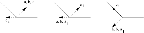
Figure 2: Brane positions in the non-supersymmetric MSSM-like models of table (18) for the wrapping choices of the set solution $(l_{4},s_{3})$; a-brane $\equiv U(3)_{a}$, b-brane $\equiv U(2)_{b}$, a₁-brane $\equiv U(1)_{c}$. The N=0 models are made from two different N=1, N^′=1 supersymmetry preserving sectors. The wrappings can be seen in table (17).

• U(1) anomalies

The analysis of U(1) anomalies shows that there is one U(1) which becomes massive though its couplings to RR fields, namely

$$U(1)^{mas}=3F_{a}+2F_{b}+F_{a_{1}}\ ,$$ (7.3)

while the hypercharge which remains massless is given by $(1/3)F_{a}-(1/2)F_{b}$. There is also a third $U(1)^{c}=(3/2)F_{a}+F_{b}-(13/2)F_{a_{1}}$ which can be broken by the vev of the tachyon singlet superpartner of $S_{0}$, and also five more U(1)’s which are linear combinations of all five U(1)’s, $U(1)^{c1},\cdots,U(1)^{c5}$ and can be broken e.g. by the vev’s of one of the singlet tachyonic superpartners of $S_{1},\cdots,S_{5}$. As there are more tachyonic singlets available in the models e.g. $S_{1},\cdots,S_{9}$, there are different choices of singlets that could be used to break the extra, beyond the hypercharge, surviving massless the Green-Schwarz mechanism U(1)’s.

• Chiral Spectrum

Most of the matter becomes massive by appropriate Yukawa couplings - denoted in table (18) by using the ”+” sign. There are only two pairs of chiral fields where the matter in each pair has opposite hypercharges with respect to the the surviving gauge group $SU(3)_{c}\times SU(2)_{L}\times U(1)_{Y}$ - that we were not able to find a mass term; denoted in table (18) by using the ”-” sign. However, even with the latter drawback it is worthwhile to examine some of its revealing phenomenology.

${\bf Matter}\hskip 28.45274pt$	$Massive$	${(SU(3)\times SU(2))}_{(Q_{a},Q_{b},Q_{a1},Q_{c1},Q_{c2},Q_{c3},Q_{c4},Q_{c5})}$	$U(1)^{Y}$
$\{Q_{L}\}\hskip 28.45274pt$	$+$	$3({3^{*}},{2^{*}})_{(-1,\ -1,\ 0,\ 0,\ 0,\ 0,\ 0,\ 0)}$	$1/6$
$\{u_{L}^{c}\}\hskip 28.45274pt$	$-$	$3({\bar{3}},1)_{(-2,\ 0,\ 0,\ 0,\ 0,\ 0,\ 0,\ 0)}$	$-2/3$
$\{d_{L}^{c}\}\hskip 28.45274pt$	$+$	$3(3,1)_{(1,\ 0,\ 0,\ -1,\ 0,\ 0,\ 0,\ 0)}$	$1/3$
$\{H_{u}\}\hskip 28.45274pt$	$+$	$3(1,{2^{*}})_{(0,\ -1,\ -1,\ 0,\ 0,\ 0,\ 0,\ 0)}$	$1/2$
$\{H_{d}^{2}\equiv H_{d}\}\hskip 28.45274pt$	$+$	$3(1,{2})_{(0,\ 1,\ 0,\ 1,\ 0,\ 0,\ 0,\ 0)}$	$-1/2$
$\{e_{L}^{+}\}\hskip 28.45274pt$	$+$	$3(1,1)_{(0,\ -2,\ 0,\ 0,\ 0,\ 0,\ 0,\ 0)}$	$1$
$\{X_{1}\}\hskip 28.45274pt$	$+$	$3(3,1)_{(1,\ 0,\ 0,\ 1,\ 0,\ 0,\ 0,\ 0,)}$	$1/3$
$\{X_{2}\}\hskip 28.45274pt$	$+$	$3(3,1)_{(1,\ 0,\ 0,\ 0,\ -1,\ 0,\ 0,\ 0)}$	$1/3$
$\{X_{3}\}\hskip 28.45274pt$	$+$	$3(3,1)_{(1,\ 0,\ 0,\ 0,\ 1,\ 0,\ 0,\ 0)}$	$1/3$
$\{X_{4}\}\hskip 28.45274pt$	$+$	$3(3,1)_{(1,\ 0,\ 0,\ 0,\ 0,\ -1,\ 0,\ 0)}$	$1/3$
$\{X_{5}\}\hskip 28.45274pt$	$+$	$3(3,1)_{(1,\ 0,\ 0,\ 0,\ 0,\ 1,\ 0,\ 0)}$	$1/3$
$\{X_{6}\}\hskip 28.45274pt$	$+$	$3(3,1)_{(1,\ 0,\ 0,\ 0,\ 0,\ 0,\ -1,\ 0)}$	$1/3$
$\{X_{7}\}\hskip 28.45274pt$	$+$	$3(3,1)_{(1,\ 0,\ 0,\ 0,\ 0,\ 0,\ 1,\ 0)}$	$1/3$
$\{X_{8}\}\hskip 28.45274pt$	$+$	$3(3,1)_{(1,\ 0,\ 0,\ 0,\ 0,\ 0,\ 0,\ -1)}$	$1/3$
$\{X_{8}\}\hskip 28.45274pt$	$+$	$3(3,1)_{(1,\ 0,\ 0,\ 0,\ 0,\ 0,\ 0,\ 1)}$	$1/3$
$\{H_{d}^{1}\equiv L\}\hskip 28.45274pt$	$+$	$3(1,2)_{(0,\ 1,\ 0,\ -1,\ 0,\ 0,\ 0,\ 0)}$	$-1/2$
$\{H_{d}^{3}\}\hskip 28.45274pt$	$+$	$3(1,2)_{(0,\ 1,\ 0,\ 0,\ -1,\ 0,\ 0,\ 0)}$	$-1/2$
$\{H_{d}^{4}\}\hskip 28.45274pt$	$+$	$3(1,2)_{(0,\ 1,\ 0,\ 0,\ 1,\ 0,\ 0,\ 0)}$	$-1/2$
$\{H_{d}^{5}\}\hskip 28.45274pt$	$+$	$3(1,2)_{(0,\ 1,\ 0,\ 0,\ 0,\ -1,\ 0,\ 0)}$	$-1/2$
$\{H_{d}^{6}\}\hskip 28.45274pt$	$+$	$3(1,2)_{(0,\ 1,\ 0,\ 0,\ 0,\ 1,\ 0,\ 0)}$	$-1/2$
$\{H_{d}^{7}\}\hskip 28.45274pt$	$+$	$3(1,2)_{(0,\ 1,\ 0,\ 0,\ 0,\ 0,\ -1,\ 0)}$	$-1/2$
$\{H_{d}^{8}\}\hskip 28.45274pt$	$+$	$3(1,2)_{(0,\ 1,\ 0,\ 0,\ 0,\ 0,\ 1,\ 0)}$	$-1/2$
$\{H_{d}^{9}\}\hskip 28.45274pt$	$+$	$3(1,2)_{(0,\ 1,\ 0,\ 0,\ 0,\ 0,\ 0,\ -1)}$	$-1/2$
$\{H_{d}^{10}\}\hskip 28.45274pt$	$+$	$3(1,2)_{(0,\ 1,\ 0,\ 0,\ 0,\ 0,\ 0,\ 1)}$	$-1/2$
$\{S_{0}\}\hskip 28.45274pt$	$+$	$3(1,1)_{(0,\ 0,\ -2,\ 0,\ 0,\ 0,\ 0,\ 0)}$	$0$
$\{S_{1}\}\hskip 28.45274pt$	$+$	$3(1,1)_{(0,\ 0,\ 1,\ -1,\ 0,\ 0,\ 0,\ 0)}$	$0$
$\{S_{2}\equiv N_{R}\}\hskip 28.45274pt$	$+$	$3(1,1)_{(0,\ 0,\ 1,\ 1,\ 0,\ 0,\ 0,\ 0)}$	$0$
$\{S_{3}\}\hskip 28.45274pt$	$+$	$3(1,1)_{(0,\ 0,\ 1,\ 0,\ -1,\ 0,\ 0,\ 0)}$	$0$
$\{S_{4}\}\hskip 28.45274pt$	$+$	$3(1,1)_{(0,\ 0,\ 1,\ 0,\ 1,\ 0,\ 0,\ 0)}$	$0$
$\{S_{5}\}\hskip 28.45274pt$	$+$	$3(1,1)_{(1,\ 0,\ 1,\ 0,\ 0,\ -1,\ 0,\ 0)}$	$0$
$\{S_{6}\}\hskip 28.45274pt$	$+$	$3(1,1)_{(0,\ 0,\ 1,\ 0,\ 0,\ 1,\ 0,\ 0)}$	$0$
$\{S_{7}\}\hskip 28.45274pt$	$+$	$3(1,1)_{(0,\ 0,\ 1,\ 0,\ 0,\ 0,\ -1,\ 0)}$	$0$
$\{S_{8}\}\hskip 28.45274pt$	$+$	$3(1,1)_{(0,\ 0,\ 1,\ 0,\ 0,\ 0,\ 1,\ 0)}$	$0$
$\{S_{9}\}\hskip 28.45274pt$	$+$	$3(1,1)_{(0,\ 0,\ 1,\ 0,\ 0,\ 0,\ 0,\ -1)}$	$0$
$\{S_{10}\}\hskip 28.45274pt$	$+$	$3(1,1)_{(0,\ 0,\ 1,\ 0,\ 0,\ 0,\ 0,\ 1)}$	$1/3$
$\{X_{0}\}\hskip 28.45274pt$	$+$	$3({\bar{3}},1)_{(-1,\ 0,\ -1,\ 0,\ 0,\ 0,\ 0,\ 0)}$	$-1/3$
$\{Q_{1}\}\hskip 28.45274pt$	$-$	$3(3,1)_{(2,\ 0,\ 0,\ 0,\ 0,\ 0,\ 0,\ 0)}$	$2/3$
$\{Q_{2}\}\hskip 28.45274pt$	$-$	$3(6^{*},1)_{(-2,\ 0,\ 0,\ 0,\ 0,\ 0,\ 0,\ 0)}$	$-2/3$
$\{P_{1}\}\hskip 28.45274pt$	$-$	$3(1,1)_{(0,\ 2,\ 0,\ 0,\ 0,\ 0,\ 0,\ 0)}$	$-1$
$\{P_{2}\}\hskip 28.45274pt$	$-$	$3(1,3^{*})_{(0,\ -2,\ 0,\ 0,\ 0,\ 0,\ 0,\ 0)}$	$+1$

Table 18: The chiral fermion spectrum of the 8-stack three generation N=1 MSSM on top of the table, in addition to three $N_{R}$’s and three pairs of $H_{u}$, $H_{d}$ chiral matter. The model is non-supersymmetric but the MSSM matter is N=1 supersymmetric. Notice the presence of extra non-susy Higgsinos $H_{d}^{k}$, k=3, .., 10.

The Yukawa couplings of the models are given by

$$Y\ =Y_{(SM)}+Y_{\mu}+Y_{X_{0}}+Y_{X_{i}},$$ (7.4)

where

$$Y_{(SM)}=\ \lambda_{d}Q_{L}d_{L}^{c}{\tilde{H}}_{d}^{2}+\lambda_{e}Le_{L}^{+}{\tilde{H}}_{d}^{2}+\lambda_{\nu}LN_{R}{\tilde{H}}_{u},$$ (7.5)

$$Y_{\mu}=\left(\lambda_{H_{d}}H_{u}H_{d}{\tilde{S}}_{1}\right)+\{\lambda_{H_{d}^{1}}LH_{u}{\tilde{S}}_{2}\}++\lambda_{H_{d}^{3}}H_{u}H_{d}^{3}{\tilde{S}}_{4}+\lambda_{H_{d}^{4}}H_{u}H_{d}^{4}{\tilde{S}}_{3}+\lambda_{H_{d}^{5}}H_{u}H_{d}^{5}{\tilde{S}}_{6}$$

$$+\lambda_{H_{d}^{6}}H_{u}H_{d}^{6}{\tilde{S}}_{5}+\lambda_{H_{d}^{7}}H_{u}H_{d}^{7}{\tilde{S}}_{8}+\lambda_{H_{d}^{8}}H_{u}H_{d}^{8}{\tilde{S}}_{7}+\lambda_{H_{d}^{9}}H_{u}H_{d}^{9}{\tilde{S}}_{10}+\lambda_{H_{d}^{10}}H_{u}H_{d}^{10}{\tilde{S}}_{9}$$

(7.6)

$$Y_{X_{0}}\ =\ \lambda_{N}X_{0}d_{L}^{c}{\tilde{N}}_{R}\ +\lambda_{X_{1}^{m}}X_{0}X_{1}{\tilde{S}}_{1}\ +\lambda_{X_{2}^{m}}X_{0}X_{2}{\tilde{S}}_{4}\ +\lambda_{X_{3}^{m}}X_{0}X_{3}{\tilde{S}}_{3}\ +\lambda_{X_{4}^{m}}X_{0}X_{4}{\tilde{S}}_{6}\ +$$

$$\lambda_{X_{5}^{m}}X_{0}X_{5}{\tilde{S}}_{5}+\lambda_{X_{6}^{m}}X_{0}X_{6}{\tilde{S}}_{8}+\lambda_{X_{7}^{m}}X_{0}X_{7}{\tilde{S}}_{7}+\lambda_{X_{8}^{m}}X_{0}X_{8}{\tilde{S}}_{10}+\lambda_{X_{9}^{m}}X_{0}X_{9}{\tilde{S}}_{9}$$

(7.7)

$$Y_{X_{i}}\ =\ \lambda_{X_{1}}Q_{L}X_{1}{\tilde{H}}_{d}^{1}+\lambda_{X_{2}}Q_{L}X_{2}{\tilde{H}}_{d}^{4}+\lambda_{X_{3}}Q_{L}X_{3}{\tilde{H}}_{d}^{3}+\lambda_{X_{4}}Q_{L}X_{4}{\tilde{H}}_{d}^{6}\ +\$$

$$\lambda_{X_{5}}Q_{L}X_{5}{\tilde{H}}_{d}^{5}\ +\ \lambda_{X_{6}}Q_{L}X_{6}{\tilde{H}}_{d}^{8}\ +\ \lambda_{X_{7}}Q_{L}X_{7}{\tilde{H}}_{d}^{7}\ +$$

$$\ \lambda_{X_{8}}Q_{L}X_{8}{\tilde{H}}_{d}^{10}\ +\ \lambda_{X_{9}}Q_{L}X_{9}{\tilde{H}}_{d}^{9}$$ (7.8)

$\bullet$ Quark, lepton and extra matter masses:

The first Yukawa term $Y_{(N=1\ SM)}$ in (7.4) generates mass terms for all SM matter but the up-quarks, where we have identify the right neutrinos with the singlets $S_{2}$. In the present models since a perturbative mass term the up-quarks is not allowed, it is interesting to engage in a short description of the phenomenology of these models. The ${\tilde{H}}_{u}$, ${\tilde{H}}_{d}^{2}$ Higgses - play the role of the corresponding two Higgs doublets in the MSSM - couple to the SM matter at tree level. The neutrinos get also a tree level mass from a Yukawa term in (7.5) as we have identify $N_{R}\equiv S_{2}$. If for example we had identify $N_{R}$ with e.g. $S_{0}$, the only mass term allowed for the neutrinos would have been the dimension eight operators that represent $(\alpha^{\prime})^{2}$ corrections coming from the exchange of massive string states

$$m_{\nu}\propto\frac{1}{M_{s}^{4}}LN_{R}\langle Q_{L}d_{L}^{c}\rangle\langle({\tilde{S}}_{2}\rangle)^{2}\ .$$ (7.9)

For values of the d-quark chiral condensate $\langle d_{R}d_{L}\rangle\propto(200\ MeV)^{3}$ and values of the

$$m_{\nu}\propto\frac{<d_{R}d_{L}>}{M^{2}}$$ (7.10)

string scale $M_{s}\propto 1-10$ TeV neutrino masses of order 0.1 - 10 eV’s, consistent with neutrino oscillation experiments are obtained. Similar terms to (7.9), that provide masses to neutrinos, appear in the context of 4D IIA toroidal orientifold 5-, 6-models of [11], [12](see also [10]) to be originating from the dimension six operators $(\alpha^{\prime})LN_{R}\langle Q_{L}u_{L}^{c}\rangle$. It appears that if the models had a low scale ${\cal O}(TeV)$ there would be a universality in the use of chiral condensate of QCD of giving masses to neutrinos. However, in the present models the string scale may not be at the TeV region, as the branes wrap in all directions; there are no compact directions transverse to all stacks of branes [17], [18].
$\bullet$ Colour triplets masses and bounds on $M_{X_{i}}$, $M_{s}$

An extended see-saw mass matrix is generated by the mixing - in (7.8) and (7.5) - between the d-quarks with the triplets $X_{i}$. If we neglect the couplings (for simplicity) by assuming that in (7.8), (7.7) respectively

$$\lambda_{X_{i}}\rightarrow 0,i\neq 1;\ \ \lambda_{X_{i}^{m}}\rightarrow 0,\ \lambda_{N}\rightarrow 0$$ (7.11)

the see-saw generates contributions to the scalar potential from the 1st term in (7.5) and the 1st term in (7.8), namely $\lambda_{d}Q_{L}d_{L}^{c}{\tilde{H}}_{d}^{2}+\lambda_{X_{1}}Q_{L}X_{1}{\tilde{H}}_{d}^{1}$ giving us mass eigenvalues for the quarks $(d_{L}^{c},X_{1})$ of order

$$m_{d}=\lambda_{d}\langle{\tilde{H}}_{d}^{2}\rangle,\ m_{X_{1}}=\frac{\lambda_{X_{1}}^{2}}{\lambda_{d}}\frac{({\langle{\tilde{H}}_{d}^{1}\rangle})^{2}}{\langle{\tilde{H}}_{d}^{2}\rangle}$$ (7.12)

In compactifications coming from intersecting branes, the couplings $\lambda_{X_{1}}\propto exp^{-A_{X_{1}}}$, ${\lambda_{d}}\propto\exp^{-A_{d}}$ depend on the corresponding worldsheet areas $A_{1}$, $A_{2}$ connecting the intersection points taking part in the Yukawa interaction. Lets us select the maximum allowed value ${A_{1}},A_{2}\rightarrow 0$ , $\lambda_{X_{1}}\rightarrow 1$, $\lambda_{d}\rightarrow 1$. Then, as the mass of the “heavy Higgs” $\tilde{H}_{d}^{1}$, may be at least greater than 126 GeV (the mass of the LHC signal of “lightest Higgs”) and since $\lambda_{d}\langle{\tilde{H}}_{d}^{2}\rangle=4.8^{+0.7}_{-0.3}$ GeV [55], we derive from (7.12) that the mass of the exotic heavy triplet $X_{1}$ should be at least :

$$colour\ triplets\ bound:m_{d}=5.5\ MeV,\ m_{X_{1}}\geq 126\ GeV\ \equiv m_{X_{1}}\geq 2.89\times 10^{6}\ GeV,$$

$$colour\ triplets\ bound:m_{d}=5.5\ MeV,\ m_{X_{1}}\geq 124\ GeV\ \equiv m_{X_{1}}\geq 2.79\times 10^{6}\ GeV,$$

The latter puts a lower bound on the string scale which is

$$M_{s}=126\ GeV,\ M_{s}\geq 2.89\times 10^{6}\ GeV\ ,$$

$$M_{s}=124\ GeV,\ M_{s}\geq 2.74\times 10^{6}\ GeV\ .$$ (7.14)

In principle, this bound can be made weaker if we allow for the exponentials in the Yukawa’s, to take non-zero values. However, in this case, we may enter the area of $10^{5}\ GeV=10^{2}\ TeV$ in which it has been argued [40] that it is possible for flavour changing neutral current to appear in non-supersymmetric models from intersecting branes. At this stage of our understanding, it looks that the choice of maximum area is picked up only on anthropic principles. The value of new “heavy quark” $M_{X_{1}}$ mass is well within the bounds predicted by ATLAS, where the search for a quark through the decay $X_{1}\rightarrow Zb$ excludes the new heavy down quark $X_{1}$ for masses below 725 GeV [19].
$\bullet$ higgsinos $\&$ $P_{1},P_{2},Q_{1},Q_{2}$ masses

The first term in (7.6) is the usual Dirac term for the Higgsinos. The second term is a mixing term between the lepton L and the Higgsino $H_{u}$ generating mixing while the rest of the terms Dirac mass terms for the rest of Higgsinos. Mass terms for the fields $P_{1}$, $P_{2}$ are given by the terms (respectively) :

$$\frac{(P_{1})^{2}({\tilde{H}}_{u})^{2}({\tilde{S}}_{1})^{2}({\tilde{S}}_{2})^{2}}{M_{s}^{6}},\ \frac{(P_{2})^{2}({\tilde{H}}_{d}^{3})^{2}({\tilde{H}}_{d}^{4})^{2}}{M_{s}^{3}}\ ,$$ (7.15)

where ${\tilde{S}}_{1}$, ${\tilde{S}}_{2}$ the scalar tachyonic superpartners of $S_{1}$, $S_{2}$ gauge fermion singlets. Apart from the u-quark for which there is no obvious perrurbative mass term, we also find that there are no mass terms for the $Q_{1}$, $Q_{2}$.

7.2 A second example of a non-susy model that accommodates the MSSM-matter using N=1 susy preserving D6-branes

An alternative example of a Standard-like model is obtained by changing the identification of fields that appear in table (18). For this purpose we identify the lepton field as $L\equiv H_{d}^{3}$. In table (19), we list the chiral structure of the N=0 models. We have not included the $S_{i}$, $X_{i}$, $Q_{i}$, $P_{i}$ fields as they are the same as the ones appearing in table (18).

${\bf Matter}\hskip 28.45274pt$	$Massive$	${(SU(3)\times SU(2))}_{(Q_{a},Q_{b},Q_{a1},Q_{c1},Q_{c2},Q_{c3},Q_{c4},Q_{c5})}\hskip 56.9055pt$	$U(1)^{Y}$
$\{Q_{L}\}\hskip 28.45274pt$	$+$	$3({3^{*}},{2^{*}})_{(-1,\ -1,\ 0,\ 0,\ 0,\ 0,\ 0,\ 0)}$	$1/6$
$\{u_{L}^{c}\}\hskip 28.45274pt$	$-$	$3(3,1)_{(2,\ 0,\ 0,\ 0,\ 0,\ 0,\ 0,\ 0)}$	$-2/3$
$\{d_{L}^{c}\}\hskip 28.45274pt$	$+$	$3(3,1)_{(1,\ 0,\ 0,\ -1,\ 0,\ 0,\ 0,\ 0)}$	$1/3$
$\{H_{u}\}\hskip 28.45274pt$	$+$	$3(1,{2^{*}})_{(0,\ -1,\ -1,\ 0,\ 0,\ 0,\ 0,\ 0)}$	$1/2$
$\{H_{d}^{2}\}\hskip 28.45274pt$	$+$	$3(1,{2})_{(0,\ 1,\ 0,\ 1,\ 0,\ 0,\ 0,\ 0)}$	$-1/2$
$\{e_{L}^{+}\}\hskip 28.45274pt$	$+$	$3(1,1)_{(0,\ -2,\ 0,\ 0,\ 0,\ 0,\ 0,\ 0)}$	$1$
$\{H_{d}^{3}\equiv L\}\hskip 28.45274pt$	$+$	$3(1,2)_{(0,\ 1,\ 0,\ 0,\ -1,\ 0,\ 0,\ 0)}$	$-1/2$
$\{S_{2}\equiv N_{R}\}\hskip 28.45274pt$	$+$	$3(1,1)_{(0,\ 0,\ 1,\ 1,\ 0,\ 0,\ 0,\ 0)}$	$0$
$\{H_{d}^{1}\}\hskip 28.45274pt$	$+$	$3(1,2)_{(0,\ 1,\ 0,\ -1,\ 0,\ 0,\ 0,\ 0)}$	$-1/2$
$\{H_{d}^{4}\}\hskip 28.45274pt$	$+$	$3(1,2)_{(0,\ 1,\ 0,\ 0,\ 1,\ 0,\ 0,\ 0)}$	$-1/2$
$\{H_{d}^{5}\}\hskip 28.45274pt$	$+$	$3(1,2)_{(0,\ 1,\ 0,\ 0,\ 0,\ -1,\ 0,\ 0)}$	$-1/2$
$\{H_{d}^{6}\}\hskip 28.45274pt$	$+$	$3(1,2)_{(0,\ 1,\ 0,\ 0,\ 0,\ 1,\ 0,\ 0)}$	$-1/2$
$\{H_{d}^{7}\}\hskip 28.45274pt$	$+$	$3(1,2)_{(0,\ 1,\ 0,\ 0,\ 0,\ 0,\ -1,\ 0)}$	$-1/2$
$\{H_{d}^{8}\}\hskip 28.45274pt$	$+$	$3(1,2)_{(0,\ 1,\ 0,\ 0,\ 0,\ 0,\ 1,\ 0)}$	$-1/2$
$\{H_{d}^{9}\}\hskip 28.45274pt$	$+$	$3(1,2)_{(0,\ 1,\ 0,\ 0,\ 0,\ 0,\ 0,\ -1)}$	$-1/2$
$\{H_{d}^{10}\}\hskip 28.45274pt$	$+$	$3(1,2)_{(0,\ 1,\ 0,\ 0,\ 0,\ 0,\ 0,\ 1)}$	$-1/2$

Table 19: A non-supersymmetric SM-like model with the three generation N=1 SM fermion spectrum on top of the table, where only the 1 pair of exotics, namely $Q_{i}$, remain massless (as also $u_{L}^{c}$ does). Also present the $X_{i}$, $S_{i}$, $Q_{i}$, $P_{i}$ fermions seen in table (18).

Yukawa couplings for the quarks, leptons and the $X_{i}$’s are given by

$${\tilde{Y}}\ ={\tilde{Y}}_{(N=1\ SM)}+{\tilde{Y}}_{\mu}+{\tilde{Y}}_{X_{0}}+{\tilde{Y}}_{X_{i}},$$ (7.16)

where

$${\tilde{Y}}_{N=1\ SM}\ =\ \lambda_{d}Q_{L}d^{c}_{L}{\tilde{H}}_{d}^{2}\ +\ \lambda_{e}Le_{L}^{+}{\tilde{H}}_{u}^{4}+\lambda_{\nu}\frac{LN_{R}{\tilde{H}}_{u}{\tilde{S}}_{o}{\tilde{S}}_{1}{\tilde{S}}_{4}}{M_{s}^{3}}$$ (7.17)

$${\tilde{Y}}_{\mu}=Y_{\mu},\ \ {\tilde{Y}}_{X_{o}}=Y_{X_{o}},\ {\tilde{Y}}_{X_{i}}=Y_{X_{i}},\$$ (7.18)

As in the models of the previous section, the non-chiral fields $Q_{i}$ $\&$ $u_{L}^{c}$ remain massless. Other N=0 SM-like models can be obtained from the one’s in table (18) by changing the assignment of right handed neutrinos to any of the singlets $S_{i}$ and/or the identification of leptons with any of the fields $H^{i}_{d}$.

8 IIA $Z_{3}\times Z_{3}$ orientifolds on the ABB lattice

$\bullet$ Spectrum rules

For the calculations on the ABB lattice in this section, we may use a different lattice basis that the one used in the rest of this work. We are using the A, B lattices found in the Appendix of [8] and in [6], where a general D6_a-brane is determined by three pairs of wrapping numbers $(n_{a},m_{a})$ along the fundamental cycles (organized into orbits) with complex structure in each $(T^{2})_{a}$-torus a=1,2,3, defined as $U_{A}=\frac{1}{2}+i\frac{\sqrt{3}}{2}$, $U_{B}=\frac{1}{2}+i\frac{1}{2\sqrt{3}}$. A generic D6_a-brane is determined by three pairs of wrapping numbers $(n_{a},m_{a})$ along the fundamental cycles of each $T^{2}$,

$$e^{A}_{1}=e^{B}_{1}=R,\ e^{A}_{2}=\frac{R}{2}+i\frac{\sqrt{3R}}{2},\ e^{B}_{2}=\frac{R}{2}+i\frac{R}{2\sqrt{3}}\ .$$ (8.1)

The massless spectrum is given in terms of the effective wrappings $({\tilde{Z}}_{a},{\tilde{Y}}_{a})$. The RR tadpoles, the cancellation of RR charge in homology, are found to be

$$\sum_{a}N_{a}{\tilde{Z}}_{a}=12,$$ (8.2)

$${\tilde{Z}}_{a}\ =\ 6n^{1}_{a}n^{2}_{a}n^{3}_{a}+3(n^{1}_{a}n^{2}_{a}m^{3}_{a}+n^{1}_{a}m^{2}_{a}n^{3}_{a}+m^{1}_{a}n^{2}_{a}n^{3}_{a})+m^{2}_{a}m^{3}_{a}n^{1}_{a}-m^{1}_{a}m^{2}_{a}m^{3}_{a}$$ (8.3)

or

$${\tilde{Z}}_{a}\ =\ 6n^{1}_{a}n^{2}_{a}n^{3}_{a}+3(\underline{n^{1}_{a}n^{2}_{a}m^{3}_{a}})+m^{2}_{a}m^{3}_{a}n^{1}_{a}-m^{1}_{a}m^{2}_{a}m^{3}_{a}\ ,$$ (8.4)

where by underline we mean all possible permutations of indices and

$${\tilde{Y}}_{a}\ =\ 3n_{a}^{1}n_{a}^{2}n_{a}^{3}+n_{a}^{1}n_{a}^{2}m_{a}^{3}+n^{1}_{a}m^{2}_{a}n^{3}_{a}-m_{a}^{1}n_{a}^{2}m_{a}^{3}-m_{a}^{1}m_{a}^{2}n_{a}^{3}-m_{a}^{1}m_{a}^{2}m_{a}^{3}\ .$$ (8.5)

${\bf Representation\hskip 28.45274pt}$	${\bf Multiplicity\hskip 28.45274pt}$
$\hskip 56.9055pt\raisebox{-3.5pt}{\hbox{\rule{0.4pt}{6.5pt}\hskip-0.4pt\rule{6.5pt}{0.4pt}\hskip-6.5pt\rule[6.5pt]{6.5pt}{0.4pt}}\rule[6.5pt]{0.4pt}{0.4pt}\hskip-0.4pt\rule{0.4pt}{6.5pt}}\hskip-6.9pt\raisebox{3.0pt}{\hbox{\rule{0.4pt}{6.5pt}\hskip-0.4pt\rule{6.5pt}{0.4pt}\hskip-6.5pt\rule[6.5pt]{6.5pt}{0.4pt}}\rule[6.5pt]{0.4pt}{0.4pt}\hskip-0.4pt\rule{0.4pt}{6.5pt}}_{L}\ =\ A_{L}\hskip 28.45274pt$	$\frac{1}{2}(I_{aa^{\prime}}+I_{a,O6})\ =\ \frac{3}{2}(Z_{a}-2Y_{a})(Z_{a}+3)\hskip 28.45274pt$
$\hskip 56.9055pt\raisebox{-0.5pt}{\hbox{\rule{0.4pt}{6.5pt}\hskip-0.4pt\rule{6.5pt}{0.4pt}\hskip-6.5pt\rule[6.5pt]{6.5pt}{0.4pt}}\rule[6.5pt]{0.4pt}{0.4pt}\hskip-0.4pt\rule{0.4pt}{6.5pt}}\hskip-0.4pt\raisebox{-0.5pt}{\hbox{\rule{0.4pt}{6.5pt}\hskip-0.4pt\rule{6.5pt}{0.4pt}\hskip-6.5pt\rule[6.5pt]{6.5pt}{0.4pt}}\rule[6.5pt]{0.4pt}{0.4pt}\hskip-0.4pt\rule{0.4pt}{6.5pt}}_{L}\ =\ S_{L}\hskip 28.45274pt$	$\frac{1}{2}(I_{aa^{\prime}}-I_{a,O6})\ =\ \frac{3}{2}(Z_{a}-2Y_{a})(Z_{a}-3)\hskip 28.45274pt$
$\hskip 56.9055pt(N_{a},{\bar{N}}_{b})_{L}\hskip 28.45274pt$	$I_{ab}\ =\ 3(Z_{a}Y_{b}-Y_{a}Z_{b})\hskip 28.45274pt$
$\hskip 56.9055pt(N_{a},N_{b})_{L}\hskip 28.45274pt$	$I_{ab^{\prime}}\ =\ 3(Z_{a}Z_{b}-Z_{a}Y_{b}-Y_{a}Z_{b})\hskip 28.45274pt$

Table 20: The massless open string spectrum in four dimensions (ABB lattice).

Table (20) contains the usual left handed bifundamental fields $(N_{a},{\bar{N}}_{b})$, $(N_{a},{N}_{b})$, as well as antisymmetric and symmetric representations of chiral open strings stretching between D6-branes and its nine images $\Omega R\Theta^{k}\omega^{l}$. Also present are massless adjoint, non-chiral, matter created by open strings stretching between the D6-branes and its $\Theta^{k}\omega^{l}$ image branes as follows :

$$(Adj)_{L}\ :\ [(m^{1})_{a}^{2}+(n^{1})_{a}^{2}+(m^{1})_{a}(n^{1})_{a}][(m^{2}_{a}m^{3}_{a})^{2}\ +\ 3m^{2}_{a}(m^{3}_{a})^{2}n^{2}\ +\ 3(m^{3}_{a})^{2}(n^{2}_{a})^{2}\ +$$

$$3(m^{2}_{a})^{2}m_{a}^{3}n_{a}^{3}+3(m^{2}_{a})^{2}(n^{3}_{a})^{2}+9m^{2}_{a}m^{3}_{a}n^{2}_{a}n^{3}_{a}+9m^{3}_{a}(n^{2}_{a})^{2}n^{3}_{a}+9m_{a}^{2}n_{a}^{2}(n^{3}_{a})^{2}+9(n^{2}_{a})^{2}(n^{3}_{a})^{2}]$$

Adjoint matter is N=1 supersymmetric as the $Z_{3}\times Z_{3}$ rotations preserve N=1 supersymmetry.

$\bullet$ Anomaly cancellation

The cancellation of cubic non-abelian gauge anomaly is proportional to

$$\sum_{b\neq a}(N_{b}Z_{a}Z_{b}-2N_{b}N_{b}Z_{b}Y_{a})+(N_{a}-4)(Z_{a}-2Y_{a})(Z_{a}+3)+(N_{a}+4)(Z_{a}-2Y_{a})(Z_{a}-3)$$ (8.7)

The anomaly is cancelled through the use of tadpole condition (8.2). The mixed non-abelian U(1) - $SU(N_{b})^{2}$ anomalies may read

$$A_{mixed}=\frac{N_{a}}{2}(I_{ab}+I_{ab^{\prime}})=\frac{N_{a}({\tilde{Z}}_{a}-2{\tilde{Y}}_{a}){\tilde{Z}}_{b}}{2}$$ (8.8)

In order to cancel these anomalies one has to make use of a generalized Green-Schwarz mechanism (GSM) as suggested in [5], [10]. The GSM application in the case of of our $Z_{3}\times Z_{3}$ orientifolds reads

$$\sum_{a}N_{a}(M_{o}-(\Omega R)M_{o})\int_{M4}B^{0}_{2}\wedge F_{a}\ \ ; \ \ (K_{o}+(\Omega R)K_{o})\int_{M4}C^{0}\wedge F_{b}\wedge F_{b}$$

$$\sum_{a}N_{a}(N_{o}-(\Omega R)N_{o})\int_{M4}B^{I}_{2}\wedge F_{a}\ \ ; (L_{o}+(\Omega R)L_{o})^{I}\int_{M4}C^{I}\wedge F_{b}\wedge F_{b}.$$ (8.9)

$$M_{o}=\sum_{orbits}m^{1}_{a}m^{2}_{a}m^{3}_{a}, K_{o} =\sum_{orbits}n^{1}_{b}n^{2}_{b}n^{3}_{b}$$

$$N_{o}=\sum_{orbits}n^{J}_{a}n^{K}_{a}m^{I}_{a} L_{o} =\sum_{orbits}n^{I}_{b}m^{J}_{b}m^{K}_{b}$$ (8.10)

$$(M_{o}-(\Omega R)M_{o})=-18({\tilde{Z}}_{a}-2{\tilde{Y}}_{a}), (K_{o}+(\Omega R)K_{o})=-3{\tilde{Z}}_{b},$$

$$(N_{o}-(\Omega R)N_{o})^{1}=-3({\tilde{Z}}_{a}-2{\tilde{Y}}_{a}), (L_{o}+(\Omega R)L_{o})^{1}=-9{\tilde{Z}}_{b},$$

$$(N_{o}-(\Omega R)N_{o})^{2}=0, (L_{o}+(\Omega R)L_{o})^{2}=-3{\tilde{Z}}_{b},$$

$$(N_{o}-(\Omega R)N_{o})^{3}=0, (L_{o}+(\Omega R)L_{o})^{3}=-3{\tilde{Z}}_{b}$$ (8.11)

It is obvious, that the couplings (8.9) have the right form to cancel the anomaly (8.8).

$\bullet$ Model Building on the ABB lattice

The choise of wrappings

$$(Z,Y)_{a} = (3,1),\ \ (Z,Y)_{b}=(1,0),\ \ (Z,Y)_{c}=(1,1),$$ (8.12)

satisfies the RR tadpoles (8.2). The associated non-susy chiral spectrum is seen on table (21).

${\bf Matter\hskip 56.9055pt}$	$(SU(3)\times SU(2))_{(Q_{a},Q_{b},Q_{c})}\hskip 56.9055pt$	$U(1)^{Y}$
$\hskip 56.9055pt\{6{\bar{Q}}_{L}\}\hskip 56.9055pt$	$3({\bar{3}},{2},1)_{(-1,\ 1,\ 0)}\hskip 56.9055pt$	$-1/6$
$\hskip 56.9055pt\{3Q_{L}\}\hskip 56.9055pt$	$6({3},{2},1)_{(1,\ 1,\ 0)}\hskip 56.9055pt$	$1/6$
$\hskip 56.9055pt\{6X_{1}+3d_{L}^{c}\}\hskip 56.9055pt$	$9({3},1,1)_{(2,\ 0,\ 0)}\hskip 56.9055pt$	$1/3$
$\hskip 56.9055pt\{6X_{2}\}\hskip 56.9055pt$	$6(3,1,1)_{(1,\ 0,\ -1)}\hskip 56.9055pt$	$-1/3$
$\hskip 56.9055pt\{3u_{c}^{L}\}\hskip 56.9055pt$	$3({\bar{3}},1,1)_{(-1,\ 0,\ -1)}\hskip 56.9055pt$	$-2/3$
$\hskip 56.9055pt\{3L\}\hskip 56.9055pt$	$3(1,2,1)_{(0,\ 1,\ -1)}\hskip 56.9055pt$	$-1/2$
$\hskip 56.9055pt\{3S_{1}+3N_{R}\}\hskip 56.9055pt$	$6(1,1,1)_{(0,\ 2,\ 0)}\hskip 56.9055pt$	$0$
$\hskip 56.9055pt\{3S_{2}\}\hskip 56.9055pt$	$3(1,{\bar{3}},1)_{(0,\ -2,\ 0)}\hskip 56.9055pt$	$0$
$\hskip 56.9055pt\{e_{R}^{c}\}\hskip 56.9055pt$	$3(1,1,1)_{(0,\ 0,\ 2)}\hskip 56.9055pt$	$1$

Table 21: A three generation non-supersymmetric chiral (open string) spectrum accommodating the MSSM fermionic matter. The hypercharge is $U(1)^{Y}=\frac{1}{3}F_{a}+\frac{1}{2}F_{c}$.

9 SPLIT SUPERSYMMETRY $\&$ D6-brane models with $sin^{2}(\theta)=\frac{3}{8}$

String Theory Intersecting D-brane models (STIB) is the natural arena for the realization of ideas on the existence of split supersymmetry (SS) [50, 51, 69] in particle physics. The SS claim [50] relies on a number of assumptions that demand :
(a) that the particle spectrum of the SM remain massless to low energies
(b) that the SM spartners become massive with a mass of the order of the supersymmetry breaking scale
(c) the gauge couplings unify at a scale near $10^{16}$ GeV
(d) there are light gauginos in the presence of gravity [Note that condition should be modified in STIBs as gauginos get a mass of order $M_{s}$.]
(e) there are light higgsinos in the presence of gravity and thus might be seen experimentally
(f) the assumption of the existence of a heavy and a light Higgs set of doublets present in the spectrum that form two chiral supermultiplets. In this section we will present models that can some times fully satisfy conditions (a), (b), (c) (d), (e).

We also note that condition (f), the existence of a Higgs light was assumed in [50] that it may be a result of a fine tuning mechanism. In models that may come from intersecting branes supersymmetric Higgs sets may appear naturally. The present D-brane models have not a supersymmetric Higgs sector. However, the Higgs system can be understood as part for the massive spectrum that organizes itself in terms of massive N=2 hypermultiplets. The Higgs fields become subsequently tachyonic in order to participate in electroweak symmetry breaking [see also similar considerations [10, 11, 12, 13]].

Conditions (a), (b), (c), (d) can be naturally obtained - in intersecting brane worlds - and in the current models. The (e), (f) conditions are harder to be obtained and may be examined in a case by case basis. Also condition (c) for a particle physics model that includes gravity - as STIBs - means that the string scale should be high and at least $10^{16}$ GeV. Condition (a) can be naturally satisfied in STIBS and there are a lot of models exhibiting only the SM spectrum at low energies. These models accommodate the SM spectrum and can be either belong to an overall non-supersymmetric model or to an overall N=1 supersymmetric model. The first case involves three generation models with supersymmetry broken at the string scale as it has been exhibited in the toroidal orientifolds in [10, 11, 12, 13] and in the previous sections as superpartners of the SM are being massive and of the order of the string scale. It is also possible to construct non-supersymmetric constructions that localize locally the N=1 supersymmetric SM spectrum and such models have been constructed in [25], [26], [20]. In particular in [26] we generalized the four stack constructions of [25] by also including a non-zero B-field flux in the models[also extending these models to their maximal extensions with gauge groups made of five and six stacks of D6-branes at the string scale]. This makes the torus tilted and allows for more general solutions in the RR tadpoles as well changing the number of N=1 Higgs supermultiplets present in the spectrum. In the four stack models constructed in [25, 26] it has been shown [52] that it is possible to accommodate the successful prediction of supersymmetric SU(5) GUTS with $sin^{2}(\theta)=3/8$ at a string scale which coincides with the unification scale of $2\cdot 10^{16}$ GeV, and all gauge coupling constants unified at $10^{16}$ GeV. Hence condition (c) is also satisfied in IBs and obviously all the D-brane models appearing in [25], [26] could form realistic D-brane split susy models as RR tadpoles has been shown to be consistently implemented in [20]and in the present work. Next, we will also show that it is also possible - in the framework of the present $Z_{3}\times Z_{3}$ orientifolds - to easily build models which satisfy conditions (a),(b),(c),(d); some models may also satisfy partially or fully the condition (e).

9.1 1st example : Split Susy (SM + $\nu_{R}$ + Higgsinos) models: “massive Gauginos” $\&$ “light Higgsinos” $\&$ $sin^{2}\theta_{W}(M_{S})=\frac{3}{8}$

In this section we will construct a deformation of the SM’s appeared in section (3.1) and table (1) where (a), (b), (c), (d), (e) conditions of split susy are satisfied. These models have the initial gauge group $U(3)\times U(2)\times U(1)$ with supersymmetry broken at $M_{s}$ and at low energy the gauge group becomes identical to the SM. The massless fermion spectrum contains the MSSM fermion matter and is given in table (22). RR tadpoles are satisfied by the choices $N_{a}=3$, $N_{b}=2$, $N_{c}=1$ and

$$(Z_{a},Y_{a})=\left(\begin{array}[]{cc}1,&1\\ \end{array}\right),\ (Z_{b},Y_{b})=\left(\begin{array}[]{cc}1,&1\\ \end{array}\right),\ (Z_{c},Y_{c})=\left(\begin{array}[]{cc}-1,&1\\ \end{array}\right)\ .$$ (9.1)

At the top of the table (22) we see the massless fermion spectrum of the N=1 SM whose corresponding superpartners are part of the massive spectrum and appear in the intersection of each corresponding fermion; hence condition (b) is satisfied.

${\bf Matter\hskip 56.9055pt}$	Intersection	$(SU(3)\times SU(2))_{(Q_{a},Q_{b},Q_{c})}\hskip 56.9055pt$	$U(1)^{Y}$
$\hskip 56.9055pt\{Q_{L}\}\hskip 56.9055pt$	$ab*$	$3({3},{2})_{(-1,\ -1,\ 0)}\hskip 56.9055pt$	$1/6$
$\hskip 56.9055pt\{u_{L}^{c}\}\hskip 56.9055pt$	$A_{a}$	$3(3,1)_{(-2,\ 0,\ 0)}\hskip 56.9055pt$	$-2/3$
$\hskip 56.9055pt\{d_{L}^{c}\}\hskip 56.9055pt$	$ac$	$3(3,1)_{(1,\ 0,\ -1)}\hskip 56.9055pt$	$1/3$
$\hskip 56.9055pt\{\ L\}\hskip 56.9055pt$	$bc$	$3(1,2)_{(0,\ 1,\ -1)}\hskip 56.9055pt$	$-1/2$
$\hskip 56.9055pt\{\ H_{d}\}\hskip 56.9055pt$	bc	$3(1,2)_{(0,\ 1,\ -1)}\hskip 56.9055pt$	$-1/2$
$\hskip 56.9055pt\{H_{u}\}\hskip 56.9055pt$	$bc*$	$3(1,{\bar{2}})_{(0,\ -1,\ -1)}\hskip 56.9055pt$	$1/2$
$\hskip 56.9055pt\{e_{L}^{+}\}\hskip 56.9055pt$	$A_{b}$	$3(1,1)_{(0,\ -2,\ 0)}\hskip 56.9055pt$	$1$
$\hskip 56.9055pt\{N_{R}\}\hskip 56.9055pt$	$S_{c}$	$9(1,1)_{(0,\ 0,\ 2)}\hskip 56.9055pt$	$0$
$\hskip 56.9055pt\{C_{1}\}\hskip 56.9055pt$	$ac$	$3(3,1)_{(1,\ 0,\ -1)}\hskip 56.9055pt$	$1/3$
$\hskip 56.9055pt\{C_{2}\}\hskip 56.9055pt$	$ac*$	$3({\bar{3}},1)_{(-1,\ 0,\ -1)}\hskip 56.9055pt$	$-1/3$

Table 22: A three generation 4D non-supersymmetric model with the chiral content of N=1 MSSM on top of the table, in addition to $N_{R}$’s. There are three pairs of $H_{u}$, $H_{d}$ Higgsinos. This model mimics models coming from gauge mediation scenarios and possess $sin^{2}\theta=3/8$ at $M_{s}$.

In order to show that at low energy only the SM remains [condition (a)]; the extra beyond the SM fermion matter and all U(1) gauge fields originally present at the string scale should become massive but the hypercharge. Hence Higginos and the exotics $C_{i}$ receive non-zero masses. The Yukawa couplings (9.2) provide masses to d,e and a Dirac term for neutrinos

$$\lambda_{d}{(Q_{L})}_{(-1,-1,0)}{(d^{c}_{L})}_{(1,0,-1)}\langle{{\tilde{H}}_{d}}\rangle\ +\ \lambda_{\nu}LN_{R}\langle{\tilde{H}}_{u}\rangle\ +\frac{\lambda_{e}}{M_{s}}Le_{L}^{c}\langle{\tilde{H}}_{d}\rangle+(\lambda_{H}H_{u}H_{d}+\lambda_{C}C_{1}C_{2})\langle{\tilde{N}}_{R}\rangle$$ (9.2)

via the previously massive tachyonic superpartners ${\tilde{H}}_{u}$, ${\tilde{H}}_{d}$ of Higgsinos $H_{u}$, $H_{d}$ as in eq. (3.4). We also note that the Higgs fields have the quantum numbers

$${\tilde{H}}_{u}=(1,2,1)_{(0,-1,-1)},\ \ {\tilde{H}}_{d}=(1,2,1)_{(0,1,1)}\ .$$ (9.3)

The pair of non-chiral colour triplets could get massive by their Yukawa coupling to the tachyonic spartner of $N_{R}$, $\langle{\tilde{N}}_{R}\rangle$ (by choosing $\lambda_{C}\sim e^{-A_{C}},\ A_{C}\rightarrow 0$) of order $M_{s}$. The Higgsinos [condition (e)] $H_{u}$, $H_{d}$, form a Dirac mass term from the Yukawa coupling

$$\lambda_{H}H_{u}H_{d}\langle{\tilde{N}}_{R}\rangle,\ \ \lambda_{H}\sim e^{-A_{hig}}\ ,$$ (9.4)

where ${\tilde{N}}_{R}$ is the scalar tachyonic superpartner of $N_{R}$. The vev of ${\tilde{N}}_{R}$ is of the order of the string scale when $A_{hig}\rightarrow 0$. Due to nature of the Yukawa coupling term [see also eqn. (3.7)] in (9.4) the Higgsino mass can be anywhere between the string scale and the scale of electroweak symmetry breaking,

$$100\ GeV<m_{(Higgino\ pair)}\leq M_{s}\ ,$$ (9.5)

which requires the areas to be $A_{min}\sim 34$, $A_{max}=0$ for the lower and upper limits of (9.5). Lets us discuss the U(1) structure. One U(1) gauge field becomes massive through its BF couplings, namely $-3F_{a}-2F_{b}-3F_{c}$, while from the extra U(1)’s that survive massless the GS mechanism; one combination of U(1)’s is the hypercharge while the third $U(1)^{add}$ gets broken by the vev of ${\tilde{N}}_{R}$.

$$U(1)^{Y}=\frac{1}{3}F_{a}-\frac{1}{2}F_{b},\ \ U(1)^{add}=F_{a}+(2/3)F_{b}-(13/9)F_{c}\ .$$ (9.6)

As the present $Z_{3}\times Z_{3}$ orientifolds involve D6-branes the gauge coupling constants are controlled by the length of the corresponding cycles that the D6-branes wrap

$$\frac{1}{\alpha_{a}}\ =\ ||l_{i}||\ ,$$ (9.7)

where $||l_{i}||$ is the length of the corresponding cycle for the i-th set of brane stacks. The canonically normalized U(1)’s as well the normalization of the abelian generators are given by

$${\tilde{U}}(1)_{a}\ =\ \frac{F_{a}}{\sqrt{2N_{a}}},\ \ Tr(T_{a}T_{b})=\frac{1}{2}\delta_{ab}$$ (9.8)

The hypercharge is given as a linear combination $Y(1)^{Y}=\sum_{i}c_{i}F_{i}$; hence in the present models the value of the weak angle is computed to be

$$\sin^{2}\theta_{W}=\frac{1}{1+4c_{2}^{2}+6c_{3}^{2}(\alpha_{2}/\alpha_{3})}\ .$$ (9.9)

Taking into account that in the present models $\alpha_{2}=\alpha_{3}$, the gauge couplings unify at $M_{s}$, we get

$$\sin^{2}\theta_{W}\stackrel{{\scriptstyle M_{s}}}{{=}}\frac{3}{8}\ .$$ (9.10)

Gauginos are massless at tree level in the present intersecting brane models and appear in the four dimensional N=4 SYM spectrum that get localized from strings having both ends on the same set of D6-branes. A mechanism for generating gaugino masses in intersecting branes - due to quantum corrections - have been put forward in [10] where non-supersymmetric toroidal orientifold models are discussed [10, 11, 12, 13]. According to this result [10], as gauginos are massless at tree level, loop corrections to gauginos proceed via massive fermions running in the loops. The order of gaugino masses is of the order of the supersymmetry breaking scale, the string scale. The same mechanism may persist in the present models. A comment is in order. The spectrum of table (22) is invariant under the exchanges $C_{1}\leftrightarrow d_{L}^{c}$, $L\leftrightarrow H_{d}$.

The D6-brane non-susy MSSM-like quiver configuration of table (22) have been simultaneously suggested in [67] (without the triplets) in a local model context, as a string theory realization of split supersymmetry (see note added in the end of this work). For further studies of spit supersymmetry see [51, 69].

9.2 2nd example : Split Susy (SM + $\nu_{R}$) models: “massive” Gauginos, “massive Higgsinos”, $sin^{2}\theta_{W}(M_{s})=3/8$

In this section, we will present models that satisfy (a),(b), (c), (d) conditions of split susy. These models are build from three stacks of intersecting D6-branes at the string scale; a variant of the models considered in section (4.1). The satisfaction of the RR tadpoles (2.11) proceeds via the choice

$$N_{a}\ =\ 3,\ \ N_{b}\ =\ 2,\ \ N_{c}\ =\ 1$$ (9.11)

and with the choice of effective wrappings

$$(Z_{a},Y_{a})=\left(\begin{array}[]{cc}1,&0\\ \end{array}\right),\ (Z_{b},Y_{b})=\left(\begin{array}[]{cc}1,&0\\ \end{array}\right),\ (Z_{c},Y_{c})=\left(\begin{array}[]{cc}-1,&0\\ \end{array}\right)$$ (9.12)

The SM fermion spectrum with three quark and lepton families is seen in table (23).

${\bf Matter\hskip 56.9055pt}$	$(SU(3)\times SU(2))_{(Q_{a},Q_{b},Q_{c})}\hskip 56.9055pt$	$U(1)^{Y}$
$\hskip 56.9055pt\{Q_{L}\}\hskip 56.9055pt$	$3(3,{2})_{(1,\ 1,\ 0)}\hskip 56.9055pt$	$1/6$
$\hskip 56.9055pt\{u_{L}^{c}\}\hskip 56.9055pt$	$3({\bar{3}},1)_{(2,\ 0,\ 0)}\hskip 56.9055pt$	$-2/3$
$\hskip 56.9055pt\{d_{L}^{c}\}\hskip 56.9055pt$	$3(3,1)_{(-1,\ 0,\ 1)}\hskip 56.9055pt$	$1/3$
$\hskip 56.9055pt\{L\}\hskip 56.9055pt$	$3(1,2)_{(0,\ -1,\ -1)}\hskip 56.9055pt$	$-1/2$
$\hskip 56.9055pt\{e_{L}^{+}\}\hskip 56.9055pt$	$3(1,1)_{(0,\ -2,\ 0)}\hskip 56.9055pt$	$1$
$\hskip 56.9055pt\{N_{R}\}\hskip 56.9055pt$	$3(1,1)_{(0,\ 0,\ 2)}\hskip 56.9055pt$	$0$

Table 23: A three generation chiral (open string) spectrum accommodating the SM. The required Higgs may come from bifundamental N=2 hypermultiplets in the N=2 $bc$, $bc^{\star}$ sectors [10, 11, 12] that may trigger brane recombination.

There is one anomalous U(1) which becomes massive

$$U(1)^{massive}=3F_{a}+2F_{b}-2F_{c}$$ (9.13)

and two anomaly free U(1)’s. One of them which can be identified

$$U(1)_{ex}\ =\ 3F_{a}+2F_{b}-\frac{13}{2}F_{c}$$ (9.14)

becomes massive by the vev of the tachyonic scalar superpartner of the right handed neutrino, leaving only the hypercharge massless to low energies

$$U(1)^{Y}=-\frac{1}{3}F_{a}+\frac{1}{2}F_{b}\ .$$ (9.15)

Light Higgsinos are not present in the models considered in this section as they are part of the massive spectrum with a mass of the order of the string scale ( having chosen $A=0$; see (9.5)); in general massive with a mass above the electroweak scale. Gauginos are expected to receive string scale masses. The strong and weak gauge couplings also unify as here also $a_{2}=a_{3}$ and $sin^{2}(M_{GUT})=3/8$.

10 Non-supersymmetric gauge unification for intersecting brane split susy models

Gauge unification for supersymmetric intersecting brane models has been examined in [52]. The evolution of the one loop renormalization group equations (ERGE) for the $SU(3)_{c}$, $SU(2)_{w}$, $U(1)_{Y}$ gauge couplings in the absence of one-loop string threshold corrections (see [35] and also [36]), $a_{2}(M_{Z})=a_{em}sin^{2}\theta(M_{Z})$, is given by

$$\frac{1}{a_{s}(M_{z})}=\frac{1}{a_{s}(M_{s})}-\frac{b_{3}}{2\pi}\ln\left(\frac{M_{Z}}{M_{s}}\right),$$

$$\frac{sin^{2}\theta_{w}(M_{Z})}{a_{em}(M_{Z})}=\frac{1}{a_{w}(M_{s})}-\frac{b_{2}}{2\pi}\ln\left(\frac{M_{Z}}{M_{s}}\right),$$

$$\frac{cos^{2}\theta_{w}(M_{Z})}{a_{em}(M_{Z})}=\frac{1}{a_{Y}(M_{s})}-\frac{b_{1}}{2\pi}\ln\left(\frac{M_{Z}}{M_{s}}\right),$$ (10.1)

$$\frac{2}{3}\frac{1}{\alpha_{s}(M_{Z})}+\frac{2sin^{2}\theta_{w}(M_{Z})-1}{\alpha_{em}(M_{Z})}=\frac{B}{2\pi}\ \ln\frac{M_{Z}}{M_{s}}\ ,$$ (10.2)

and $B=-(\frac{2}{3}b_{3}+b_{2}-b_{Y})$; $b_{3}$, $b_{2}$, $b_{1}$ are the $\beta$-function coefficients for strong, weak and hypercharge gauge couplings. For a theory which accommodates the SM and a number of extra particles below a scale $M_{s}$

$$(b_{1},\ b_{2},\ b_{3})\ =\ (\frac{20}{9}n_{G}+\frac{1}{6}n_{H}+N_{1},\ \frac{4}{3}n_{G}+\frac{1}{6}n_{H}+N_{2}-\frac{22}{3},\ \frac{4}{3}n_{G}-11+N_{3}),$$ (10.3)

where $N_{1},N_{2},N_{3}$ the contribution of the beyond the SM particles; the rest of the terms in (10.3) are the Standard model contributions; $n_{G}$ the number of generations; $n_{H}$ the number of Higgses. Lets us now examine gauge coupling unification using the MSSM-matter like models of table (22) as a representative example. They are non-supersymmetric but they respect $sin^{2}(\theta_{W})=3/8$ at the unification scale, as $a_{2}=a_{3}$. This implies that at the unification scale where the gauge couplings $SU(2)_{w}$, $SU(3)_{c}$ meet, we have the standard SU(5) relation

$$(5/3)a_{Y}=a_{s}=a_{w}=a_{2}=a_{3}$$ (10.4)

This relation ‘solves’ the following eqn.

$$\frac{1}{a_{Y}}=\frac{2}{3}\frac{1}{a_{2}}+\frac{1}{a_{w}}\ .$$ (10.5)

Remember that in traditional GUTS one has to normalize under SU(5) the RG equations, to achieve unification. On the contrary, take a a representative example the models of table (22), supersymmetry is already broken at the string scale and the theory is non-supersymmetric all along to low energies of electroweak order. The full massless spectrum of the model contains, the usual SM and nine right handed neutrinos (all with the same U(1) charges), in addition to three pairs of $H_{u}$, $H_{d}$ higgsinos $\&$ gauginos $\&$ three vector pairs of exotic SU(3) triplets in addition to two N=1 adjoint hypermultiplets [see eqn. (2.18)]; one particle in the adjoint of SU(3) (an octet) and one in the adjoint of SU(2)(a triplet). We are using the central values [54]

$$M_{z}=91.1876\ GeV, \alpha_{em}(M_{z})^{-1}=127.916$$

$$\alpha_{3}(Mz)=0.1184, sin^{2}(\theta_{Z})=0.23113\ .$$ (10.6)

Depending on the scale at which, matter becomes massive and decouples from the Wilsonian effective action, we can envisage different unification scenarios. In all cases, the gauginos receive [10] a typical mass of the order of the string scale and there will be no contribution to (10.3) in all scenarios.

$\bullet$ $\bullet$ 1st scenario : Non-susy string models with only the SM $\&$ three pairs of Higgses at low energies

1st variant  $n_{H}=6$

In this scenario the higgsinos $\&$ vector triplets receive string scale masses from Yukawa’s in eq. (9.2). Let us also suppose, for the purposes of this section, that the adjoint matter receives string scale masses by some yet unknown mechanism. Then below $M_{s}$ and substituting $n_{G}=3$, $n_{H}=6$ in eqn’s (10.3)

$$(b_{1},b_{2},b_{3})=(\frac{23}{3},-\frac{7}{3},-7),\ B=\ \frac{44}{3},\ \ a_{2}(M_{s})\ =\ a_{3}(M_{s})\approx\ 0.025\ .$$ (10.7)

The values of $a_{2}$, $a_{3}$ agree up to an error of 2.68 $\%$ as a result of using the experimental values of (10.6) in the RG eqn’s (10.1). Plugging them in (10.2), we find that the gauge couplings unify at the scale

$$M_{s}\ =\ 5.03385\cdot 10^{13}\ GeV\approx 5.03\cdot 10^{13}\ GeV;B=\frac{44}{3}$$ (10.8)

as can be seen in figure (3).

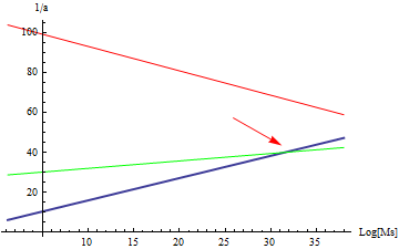
Figure 3: 1st scenario : One loop gauge running of the couplings a^-1 as a function of $Log_{10}(E/GeV)$ for the non-susy MSSM model of table (22) at $M_{s}\approx 5.03\times 10^{13}$  GeV. The head of the arrow indicates the unification point. The spectrum includes the SM $\&$ 3 pairs of Higgses at low energy. The unification point does not change if the higgses become one or three.

2nd variant  $n_{H}=1\ or\ 3$

Suppose now that only one Higgs survives at low energy (as in the SM). In this case we get the usual SM contributions

$$n_{H}=1,\ (b_{1},b_{2},b_{3})=(\frac{41}{6},-\frac{19}{6},-7),$$ (10.9)

and $B=\frac{44}{3}$ as before and $a_{2}$, $a_{3}$ agree up to an error 12.2 $\%$; $a_{2}=a_{3}\approx 0.023$. As the unification scale depends on experimental data (10.6) and B, the value of the unification scale is the same as in (10.8). Notice that it is unlikely that only one Higgs could survive massless to low energy in the present models as the Higgses appear at a single intersection with multiplicity three (3). However, this is not the case within the SM-like non-sypersymmetric models of [11], [12], [10] based on toroidal IIA orientifolds, where the number of Higgses at low energy can be one. If the minimal number of Higgses at an intersection which survives to low energies, as in split supersymmetry models of table (22) this translates to

$$n_{H}=3,\ (b_{1},b_{2},b_{3})=(\frac{43}{6},-\frac{17}{6},-7),\ B=\frac{44}{3}$$ (10.10)

and $a_{2}=a_{3}=0.023$ agree up to 8.3 $\%$. Thus with

$$SM\ \&\ \#higgs=1,3,6\ \Longrightarrow\ M_{s}\ =\ 5.03\times 10^{13}\ GeV\ .$$ (10.11)

Thus “in non-supersymmetric models coming from intersecting branes, if the SM survives at low energy below the string scale and the number of higgses is one, three or six, then always the unification scale of the strong and weak coupling occurs at the same point $M_{s}=5.03\times 10^{13}$ GeV (since the difference $-b_{2}+b_{1}$ is in all cases equal to the constant $10$ and $B=44/3$).
$\bullet$ $\bullet$ 2nd scenario : Non-susy string models with only the SM $\&$ three pairs of Higgses $\&$ minimal adjoint matter at low energies

In this case, we imagine a scenario where the extra triplets $C_{1}$, $C_{2}$ receive a mass of the order of the string scale from the vev of $\nu_{R}$’s and the Higgsinos receive a Dirac mass term (assuming that it is of order $M_{s}$) as in (9.2). As a consequence, at low energies only the SM and three pairs of Higgses survive. The models also accommodate the non-chiral adjoint matter which preserves N=1 supersymmetry; one adjoint fermion from SU(3) and another one in the adjoint of SU(2) (2.19). The $\beta$-functions become $(b_{1},b_{2},b_{3})=(\frac{20}{3}+2,-\frac{7}{3}+2,-7+2)=(\frac{23}{3},-\frac{1}{3},-5)$. Then using (10.6) in (10.2)

$$a_{3}=a_{2}\approx 0.022,\ \ \ B=\frac{34}{3}$$ (10.12)

The values of $a_{2}$, $a_{3}$ agree up to an error of 4.35 $\%$ as a result of using the experimental values of (10.6) in the RG eqn’s (10.1). We find

$$M_{s}=1.43027\cdot 10^{17}\ GeV\approx 1.43\times 10^{17}\ GeV\ .$$ (10.13)

The gauge couplings $a_{3}$, $a_{2}$ unify at the scale $M_{s}$ as seen in figure (4).

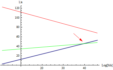
Figure 4: 2nd scenario : Unification in the non-susy model of table (22). The spectrum includes SM $\&$ 3 pairs of Higgses $\&$ adjoint fermions (one SU(3) adj + one SU(2) adj). Ms $\sim 1.43\cdot 10^{17}$ GeV.

.

$\bullet$ $\bullet$ 3rd scenario : Non-susy string models with only the SM $\&$ Higgses $\&$ adjoint matter $\&$ 3 pairs of Higgsinos at low energies

If Higgsinos receive the suppressed mass (9.5) and survive to the electroweak scale then in addition to the matter of the 1st scenario, we may add the three pair of Higgsinos contribution. Then $(b_{1},b_{2},b_{3})=(\frac{29}{3},-\frac{1}{3}+2,-7+2)$; +2 the contribution from the N=1 adjoint matter. As $B=\frac{34}{3}$ the unification scale does not change and is equal to (10.13).
$\bullet$ $\bullet$ 4th scenario : Non-susy string models with only the SM $\&$ Higgsinos $\&$ 3 pairs of Higgses at low energy
Suppose that in the 3rd scenario, the adjoint matter is getting massive by an unknown mechanism. In this case we can neglect the contribution +2 of the adjoint matter, thus getting $(b_{1},b_{2},b_{3})=(\frac{29}{3},-\frac{1}{3},-7)$; $B=44/3.$ Unification occurs at the scale given in (10.8) as the value of B is the same in the 1st scenario.

The 2nd $\&$ 3rd scenarios appear to be the most natural from the physical point of view, since the high scale of unification, keeps the proton stable.

11 Conclusions and outlook

In this work, we have presented the systematic construction of the first four dimensional three family non-supersymmetric MSSM-like models that contain models which possess the spectrum of the MSSM fermions. The models explore the details of the construction presented in [8], where mostly GUT theories were described and where model constructions are described in terms of the “effective” wrappings $(Z,Y)$. The Higgs scalars are coming from previously massive bosons that become tachyonic during electroweak symmetry breaking [10, 11, 12]. The intersection numbers that describe the number of particles at an intersection is always a multiple of three by construction. The gauge group of the models is exactly $SU(3)_{c}\times SU(2)_{w}\times U(1)_{Y}$. Any extra gauge group factors beyond the SM one, always are broken by available gauge singlets. In its minimal construction, the particle content is made from the usual chiral SM matter and pairs of up, down higgsinos. Right handed neutrinos always appear, as always happens, at intersecting brane constructions. Previous non-susy string models like the ones in toroidal orientifolds [10, 11, 12], have the baryon number a global gauged symmetry valid to low energies and thus proton was stable (see also [20]). In this respect, we examined gauge coupling unification in the simplest MSSM-like model made from 3-stacks of intersecting D6 branes, where the MSSM fermions live together with two N=1 SUSY adjoint multiplets, an octet of SU(3)_c and a 3-plet of SU(2)_W. The most appealing scenario has a unification scale $\sim 10^{17}$ GeV, thus safeguarding the proton and avoiding dimension six operators [22]. It supports the existence of either the MSSM matter accompanied by adjoint matter up to $M_{s}$ or supermassive higgsinos ($\sim M_{s}$) and surviving to low energies SM matter and light adjoints. Always, there are 3 pairs of higgses ${\tilde{H}}_{u}$, ${\tilde{H}}_{d}$ present.
$\bullet$ Proton decay
The models are safe against proton decay. Take as an example the split susy models of table (22). The dimension six baryon number violating couplings [64] $Q_{L}Q_{L}Q_{L}L$ and $u_{L}^{c}u_{L}^{c}d_{L}^{c}e_{L}^{+}$ are not allowed in perturbation theory by charge conservation. They could be in principle generated by an M-instanton [48] with wrappings (X,Y) for which obeys

$$I_{Ma}-I_{Ma^{\star}}=-1,\ I_{Mb}-I_{Mb^{\star}}=-1,I_{Mc}-I_{Mc^{\star}}=-1,$$ (11.1)

For the a-, b- branes this requires that either $3(X-Y)=0,3Y=1$ or $3(X-Y)=-1,X=Y$ conditions are satisfied. However there is no such soultion as X, Y take integer values.

We started our investigation for the construction of three generation N=0 string models by starting with the simplest construction that could accommodate the Standard Model gauge group that is using three stacks. At 3- /5-stacks we found N=0 supersymmetric vacua with the chiral fermion spectrum of the N=1 MSSM, with 3 species of right handed neutrinos and 3 pairs of chiral fermions $H_{u}$, $H_{d}$ that play the role of the MSSM Higgsinos. These models break to only the SM at low energy. In all constructions, symmetric/antisymmetric representations are present, and always the up-quark is massless at tree level; its mass may come through instanton corrections [48], [49], [28].
$\bullet$ K-theory constraints
The K-theory constraints, seen also as calculating the global gauge anomaly using a D-brane probe [62], are related to the existence of the SU(2) global gauge anomaly when there is an odd number of D=4 fermions charged in the fundamental representation [63]. As in all of our models there is an even number of fermion doublets the models are K-theory anomaly free.
$\bullet$ Split Supersymmetry Models
Models considered in the last sections of our work, show us that in intersecting brane worlds it would be possible to construct models with the characteristics of split supersymmetry that not only can drive us to a successful prediction $sin^{2}\theta=3/8$ of the SU(5) GUT value for the Weinberg angle at the unification/sting scale $M_{s}$ but also incorporate light Higgsinos and string (GUT) scale gauginos. We found models [table (22)] that the spectrum is minimal as it has only the SM and the higgsinos surviving massless below the string scale (with three pairs of Higgses and three right handed neutrinos) . This is promising against other constructions (even the existing N=1 one’s) where either the SM appears with incomplete spectrum or a lot of chiral massless matter remaining to low energies, as it can drives us closer to an exact implementation of split supersymmetry [67] scenario in intersecting D-brane models by attempting to construct, in the future, models which will be the N=1 supersymmetric implementation of the present N=0 models, with the underlying N =1 SUSY, spontaneously broken to N=0. In this case, important issues related the soft term structures and the constraint [56] $tan\beta=1$, that appears to be consistent with the “existence of one light Higgs” condition may be examined, as non-supersymmetric string models from intersecting D6-branes obey it as well [57].
$\bullet$ Dark matter, Gauge hierarchy, Unification
Nevertheless the models of this work they are possess dark matter candidates, since as suggested in [65] [66] the neutral components of higgsinos in a small mixing with the binos in models where higgsinos are present [e.g those in table (22)] can serve well this purpose. Furthermore [65], if there are additional singlet fermions in the theory, with Yukawa couplings to the Higgsino’s and the Higgs then the DM particle can then be an admixture of the singlet and neutral Higgsino components. The latter case, could get realized in the 8-stack quasi-supersymmetric (QS) models of table (18) as the coupling $(H_{u})(\langle{\tilde{H}}_{d}\rangle)^{2}\langle S_{1}\rangle)$ exists. In the latter models supersymmetry may be shown to be broken by a variation [24] of the angles between the branes. QS models with the split susy properties and proton stability and a gauged baryon number appeared in [20]. In non-supersymmetric models one expects quadratic loop corrections to the EW Higgs masses to appear as the low energy manifestation of the gauge hierarchy problem. Indeed as QW models possess N=1 supersymmetric sectors for particular choices of wrapping numbers, quadratic Higgs divergences may cancel at one loop [24] (non-necessarily higher as it is not known). Thus a full solution to the gauge hierarchy at the weak scale remains an open issue in the QS classes of split non-supersymmetric models. Finally, it is remarkable that in non-susy models from intersecting brane worlds, where $sin^{2}(M_{s})=3/8$, the unification scale remains the same $5.03\times 10^{13}$ when the number of surviving higgses is one (1), two (2) or three (3).

Acknowledgments

I am grateful to I. Antoniadis, G. Athanasiu, R. Blumenhagen, S. Dimopoulos, M. Douglas, N. Tracas, E. Floratos, G. Honecker, L. Ibanez, G. Kane, I. Klebanov, B. Körs, A. Lahanas, C. Munoz, T. Ott, and A. Uranga for useful discussions. The author wishes to thank the High Energy groups of Harvard, Princeton, Rutgers, Stanford, Kavli/UCSB, UCSB and Caltech for their warm hospitality where this work was completed. This work was supported by the programme “Pythagoras I”.

Note added

While the revised work of hep-th/0406258v3 was finishing in Nov. 2004 and were being prepared for submission we noticed [67] that also proposed the existence of split supersymmetry scenarios in string theory. In fact the local SM brane quiver configuration used in model A of [67] is the one appearing within the global string spectrum configurations of sections (4.1) and (8.2) of this work. The main bulk of this work, including the parts 1-7 appeared in hep-th in 29th June 2004. Since then, our classification MSSM (SM+Higgsinos) stringy quiver structures appearing in tables 1, 3, 9, have been also used by the authors of [71] in their tables 4, 5, 7 respectively, in order to discuss instanton generation of missing mass couplings of matter in antisymmetric/symmetric representations in a local model context. Also our three stack MSSM quiver of table 1 and the four stack MSSM quiver of table 9, have been used in [72] in their search for model quiver embeddings from Gepner models in sections 4.1, 4.2.6 of their work respectively. At the present hep-th/0406258v4, we have added new material in sections 7.1 and added the new sections 8, 10.

12 Appendix A: Wrapping $\#$’s for the minimal MSSM matter model

Wrappings, subject to the interchanges (4.6), generating the SM’s of table (3) may be seen in tables (24), (25), (26).

$Brane$	$\hskip 56.9055pt(n^{1},m^{1})\times(n^{2},m^{2})\times(n^{3},m^{3})$
$\{a\}$	$(0,\ 1)\times(1,\ 0)\times(0,\ -1)$
$\{b\}$	$(1,\ 0)\times(1,\ 1)\times(-1,-1)$
$\{c\}$	$(1,\ \ 1)\times(1,\ 1)\times(1,\ \ 0)$

Table 24: Wrapping numbers in the three stack D6-brane N=0 SMs of table (3). These wrappings come from the change $(n,m)_{a}\leftrightarrow(n,m)_{b}$ in the wrappings of table (5).

$Brane$	$\hskip 56.9055pt(n^{1},m^{1})\times(n^{2},m^{2})\times(n^{3},m^{3})$
$\{a\}$	$(0,\ -1)\times(0,\ 1)\times(1,\ 0)$
$\{b\}$	$(-1,\ -1)\times(1,\ 0)\times(1,1)$
$\{c\}$	$(1,\ \ 0)\times(1,\ 1)\times(1,\ \ 1)$

Table 25: Wrapping numbers in the three stack N=0 SMs of table (3). These wrappings come from the change $(n,m)_{a}\leftrightarrow(n,m)_{c}$ in the wrappings of table (5).

$Brane$	$\hskip 56.9055pt(n^{1},m^{1})\times(n^{2},m^{2})\times(n^{3},m^{3})$
$\{a\}$	$(1,\ 0)\times(0,\ -1)\times(0,\ 1)$
$\{b\}$	$(1,\ 1)\times(-1,\ -1)\times(1,0)$
$\{c\}$	$(1,\ \ 1)\times(1,\ 0)\times(1,\ \ 1)$

Table 26: Wrapping numbers in the three stack SMs of table (3). These wrappings come from the change $(n,m)_{b}\leftrightarrow(n,m)_{c}$ in the wrappings of table (5).

13 Appendix B : Wrapping $\#$’s for 5-stack MSSM-matter models

In this appendix, we apply the exchanges (4.6) to the wrappings of table (12). The resulting models have the same spectrum as the N=0 five stack Standard Models of table (11). These choices of wrappings can be seen in tables (27), (28), (29).

$Brane$	$\hskip 56.9055pt(n^{1},m^{1})(n^{2},m^{2})(n^{3},m^{3})$
$\{a\}$	$(1,\ 0)(1,\ 1)(-1,\ -1)$
$\{b\}$	$(0,\ 1)(1,\ 0)(0,-1)$
$\{c\}$	$(1,\ \ 0)(1,\ 1)(-1,\ \ -1)$
$\{d\}$	$(1,\ 0)(1,\ 1)(1,\ 1)$
$\{e\}$	$(1,\ 1)(1,\ 1)(1,\ 0)$

Table 27: Wrapping numbers responsible for the N=0 five stack 4D three generation intersecting D6-brane SMs of table (11). These models are derived from table (12) by the interchange $(n,m)_{a}\leftrightarrow(n,m)_{b}$.

$Brane$	$\hskip 56.9055pt(n^{1},m^{1})(n^{2},m^{2})(n^{3},m^{3})$
$\{a\}$	$(-1,\ -1)(1,\ 0)(1,\ 1)$
$\{b\}$	$(0,\ -1)(0,\ 1)(1,0)$
$\{c\}$	$(-1,\ \ -1)(1,\ 0)(1,\ \ 1)$
$\{d\}$	$(1,\ 1)(1,\ 0)(1,\ 1)$
$\{e\}$	$(1,\ 0)(1,\ 1)(1,\ 1)$

Table 28: Wrapping numbers responsible the N=0 five stack 4D three generation intersecting D6-brane SMs of table (11). These models are derived from table (12) by the interchange $(n,m)_{a}\leftrightarrow(n,m)_{c}$.

$Brane$	$\hskip 56.9055pt(n^{1},m^{1})(n^{2},m^{2})(n^{3},m^{3})$
$\{a\}$	$(1,\ 1)(-1,\ -1)(1,\ 0)$
$\{b\}$	$(1,\ 0)(0,\ -1)(0,1)$
$\{c\}$	$(1,\ \ 1)(-1,\ -1)(1,\ \ 0)$
$\{d\}$	$(1,\ 1)(1,\ 1)(1,\ 0)$
$\{e\}$	$(1,\ 1)(1,\ 0)(1,\ 1)$

Table 29: Wrapping numbers responsible for the N=0 five stack 4D three generation intersecting D6-brane SMs of table (11). These models are derived from table (12) by the interchange $(n,m)_{b}\leftrightarrow(n,m)_{c}$.

14 Appendix C: $L\leftrightarrow H_{d}$ 5-stack MSSM matter model

$\bullet$ Model C

The spectrum of the new N=0 three generation models appearing in this appendix is derived from the exchange (6.14) on the five stack models of table (11). The spectrum can be seen in table (30). The Yukawa couplings for the quarks, leptons are given by

${\bf Matter\ \ for\ \ Y^{1}}$	$Y^{1}$	$(SU(3)\times SU(2))_{(Q_{a},\ Q_{b},\ Q_{c},\ Q_{d},\ Q_{e})}\hskip 56.9055pt$
$\{Q_{L}\}$	$1/6$	$3(3,{\bar{2}})_{(-1,\ 1,\ 0,\ 0,\ 0)}$
$\{u_{L}^{c}\}$	$-2/3$	$3({\bar{3}},1)_{(-2,\ 0,\ 0,\ 0,\ 0)}$
$\{e_{L}^{+}\}$	$1$	$3(1,1)_{(0,\ 2,\ 0,\ 0,\ 0)}$
$\{d_{L}^{c}\}$	$1/3$	$3(1,1)_{(1,\ 0,\ 0,\ 1,\ 0)}$
$\{H_{u}\}$	$1/2$	$3(1,2)_{(0,\ 1,\ -1,\ 0,\ 0)}$
$\{H_{d}\}$	$-1/2$	$3(1,{2})_{(0,\ -1,\ 0,\ 1,\ 0)}$
$\{L\}$	$-1/2$	$3(1,{2})_{(0,\ -1,\ 0,\ 0,\ 1)}$
$\{S_{3}\equiv\nu_{L}^{c}\}$	$0$	$3(1,1)_{(0,\ 0,\ 1,\ 1,\ 0)}$
$\{S_{1}\}$	$0$	$3(3,1)_{(0,\ 0,\ 0,\ -2,\ 0)}$
$\{S_{2}\}$	$0$	$3(3,1)_{(0,\ 0,\ 0,\ 0,\ -2)}$
$\{S_{4}\}$	$0$	$3(1,1)_{(0,\ 0,\ 1,\ 0,\ 1)}$
$\{S_{5}\}$	$0$	$6(1,1)_{(0,\ 0,\ 0,\ -1,\ -1)}$
$\{X_{1}\}$	$-1/3$	$3({\bar{3}},1)_{(-1,\ 0,\ -1,\ 0,\ 0)}$
$\{X_{2}\}$	$1/3$	$3(3,1)_{(1,\ 0,\ 0,\ 0,\ 1)}$

Table 30: The three generation N=0 SM chiral spectrum from from five stacks of intersecting branes with its chiral spectrum with three pairs of Higgsinos. On the top of the table the chiral structure of N=1 SM with right handed neutrinos. The middle part exhibits the extra gauge singlets while the bottom part includes the triplet exotics. These models can come from the models of table (11) by the exchange (6.14).

$$Y_{(table\ \ref{newmode0})}\ =\ \lambda_{d}Q_{L}d_{L}^{c}H_{d}^{H}S_{5}^{H}/M_{s}\ +\ \lambda_{e}Le_{L}^{+}H_{d}^{H}S_{5}^{H}/M_{s}\ +\ \lambda_{\nu}L\nu_{L}^{c}H_{u}^{H}S_{5}^{H}/M_{s}\ +\$$

$$X_{1}X_{2}(\lambda_{x}^{(1)}S_{4}^{H}S_{2}^{H}+\lambda_{x}^{(2)}S_{3}^{H}S_{5}^{H})/M_{s}\ ,$$

(14.1)

where the superscript $H$ denotes the tachyonic scalar superpartner of the corresponding fermion. These models allow for a universal dependence of the masses of all the quarks and leptons on the tachyonic Higgs vev of the superpartner of $S_{5}$. The fermions $H_{u}$, $H_{d}$ get massive by the following Yukawa terms

$$H_{u}H_{d}(\lambda_{\mu}^{(1)}S_{3}^{H}S_{1}^{H}+\lambda_{\mu}^{(2)}S_{4}^{H}S_{5}^{H})/M_{s}$$ (14.2)

15 Appendix D: $d^{c}_{L}\leftrightarrow X_{2}$ 5-stack MSSM matter model

$\bullet$ Model D

The spectrum of the new N=0 three generation models appearing in this appendix is derived from the exchange (6.15) on the five stack models of table (11). It can be seen in table (31).

${\bf Matter\ \ for\ \ Y^{1}}$	$Y^{1}$	$(SU(3)\times SU(2))_{(Q_{a},\ Q_{b},\ Q_{c},\ Q_{d},\ Q_{e})}\hskip 56.9055pt$
$\{Q_{L}\}$	$1/6$	$3(3,{\bar{2}})_{(-1,\ 1,\ 0,\ 0,\ 0)}$
$\{u_{L}^{c}\}$	$-2/3$	$3({\bar{3}},1)_{(-2,\ 0,\ 0,\ 0,\ 0)}$
$\{e_{L}^{+}\}$	$1$	$3(1,1)_{(0,\ 2,\ 0,\ 0,\ 0)}$
$\{d_{L}^{c}\}$	$1/3$	$3(1,1)_{(1,\ 0,\ 0,\ 0,\ 1)}$
$\{H_{u}\}$	$1/2$	$3(1,2)_{(0,\ 1,\ -1,\ 0,\ 0)}$
$\{H_{d}\}$	$-1/2$	$3(1,{2})_{(0,\ -1,\ 0,\ 0,\ 1)}$
$\{L\}$	$-1/2$	$3(1,{2})_{(0,\ -1,\ 0,\ 1,\ 0)}$
$\{S_{3}\equiv\nu_{L}^{c}\}$	$0$	$3(1,1)_{(0,\ 0,\ 1,\ 1,\ 0)}$
$\{S_{1}\}$	$0$	$3(3,1)_{(0,\ 0,\ 0,\ -2,\ 0)}$
$\{S_{2}\}$	$0$	$3(3,1)_{(0,\ 0,\ 0,\ 0,\ -2)}$
$\{S_{4}\}$	$0$	$3(1,1)_{(0,\ 0,\ 1,\ 0,\ 1)}$
$\{S_{5}\}$	$0$	$6(1,1)_{(0,\ 0,\ 0,\ -1,\ -1)}$
$\{X_{1}\}$	$-1/3$	$3({\bar{3}},1)_{(-1,\ 0,\ -1,\ 0,\ 0)}$
$\{X_{2}\}$	$1/3$	$3(3,1)_{(1,\ 0,\ 0,\ 1,\ 0)}$

Table 31: The three generation N=1 SM from from five stacks of intersecting branes with its chiral spectrum with three pairs of Higgsinos and right neutrinos. On the top of the table the chiral structure of N=1 SM. The middle part exhibits the gauge singlets while the bottom part includes the triplet exotics. These models can come from the models of table (11) by the exchange (6.15).

Yukawa’s for the quarks, leptons, and the $X_{i}$ triplets are given by

$$Y_{(table\ \ref{toraer1})}\ =\ \lambda_{d}Q_{L}d_{L}^{c}H_{d}^{H}S_{2}^{H}/M_{s}\ +\ \lambda_{e}Le_{L}^{+}H_{d}^{H}S_{5}^{H}/M_{s}\ +\ \lambda_{\nu}L\nu_{L}^{c}H_{u}^{H}S_{1}^{H}/M_{s}\ +\$$

$$X_{1}X_{2}(\lambda_{x}^{(1)}S_{4}^{H}S_{5}^{H}+\lambda_{x}^{(2)}S_{3}^{H}S_{1}^{H})/M_{s}\ +\ H_{u}H_{d}(\lambda_{\mu}^{(1)}S_{4}^{H}S_{2}^{H}+\lambda_{\mu}^{(2)}S_{3}^{H}S_{5}^{H})/M_{s}$$ (15.1)

In fact, if $\langle S_{5}^{H}\rangle\approx\langle S_{2}^{H}\rangle\approx\langle S_{1}^{H}\rangle\approx M_{s}$, then the masses of the quarks and leptons depend universally on the scale of the electroweak symmetry breaking, assuming $\langle H_{u}\rangle\approx\langle H_{d}\rangle$. The “Higgsinos” $H_{u}$, $H_{d}$, also get a non-zero mass from the last term in (15.1).

References

- [1] For reviews see : C. Angelantonj and A. Sagnotti, Phys. Rept. 371 (2002) 1: Er-ibid. 376 (2003) 339, [arXiv:hep-th/0204089]; K. R. Dienes, Phys. Rept. 287 (1997) 447, [arXiv:hep-th/9602045]; A. Faraggi, [arXiv:hep-ph/9707311]
- [2] R. Blumenhagen, B. K¨ors, D. L¨ust, S. Stieberger, Phys. Rept. 445, 1 (2007) [hep-th/0610327]. R. Blumenhagen, B. Körs and D. Lüst, JHEP 0102 (2001) 030, [arXiv:hep-th/0012156]; D. Lüst, Class. Quant. Grav. 21:S1399-1424, 2004, [arXiv:hep-th/0401156]
- [3] C. Angelantonj, I. Antoniadis, E. Dudas and A. Sagnotti, Phys. Lett. B489 (2000) 223, [arXiv:hep-th/0007090]
- [4] M. Larosa and G. Pradisi, Nucl. Phys. B 667, 261 (2003) [hep-th/0305224].
- [5] G. Aldazabal, S. Franco, L. E. Ibanez, R. Rabadan, A. M. Uranga J.Math. Phys. 42 (2001) 3103, hep-th/0011073
- [6] R. Blumenhagen, B. Körs, D. Lüst and T. Ott, “The Standard Model from Stable Intersecting Brane World Orbifolds”, Nucl. Phys. B616 (2001) 3, [arXiv:hep-th/0107138]
- [7] J. R. Ellis, P. Kanti and D. V. Nanopoulos, Nucl. Phys. B 647, 235 (2002) [hep-th/0206087].
- [8] C. Kokorelis, “Standard model compactifications of IIA Z(3) x Z(3) orientifolds from intersecting D6-branes,” Nucl. Phys. B 732, 341 (2006) [hep-th/0412035].
- [9] M. Cvetic, G. Shiu, A. M. Uranga, Nucl.Phys. B615 (2001) 3, [arXiv:hep-th/0107166]; M. Cvetic, G. Shiu, A. M. Uranga, Phys. Rev. Lett. 87 (2001) 201801, [arXiv:hep-th/0107166]; M. Cvetic, T. Li, T. Liu, “Supersymmetric Pati-Salam models fromintersecting D6-branes: A Road to the Standard Model”, [arXiv:hep-th/0403061]
- [10] L. E. Ibáñez, F. Marchesano and R. Rabadán, “Getting just the standard model at intersecting branes” JHEP, 0111 (2001) 002, [arXiv:hep-th/0105155]
- [11] C. Kokorelis,“New Standard Model Vacua from Intersecting Branes”, JHEP 09 (2002) 029, [arXiv:hep-th/0205147]
- [12] C. Kokorelis, “Exact Standard Model Compactifications from Intersecting Branes”, JHEP 08 (2002) 036, [arXiv:hep-th/0206108]
-
[13]
For detailed realizations of the Pati-Salam structure
in intersecting brane worlds see :
C. Kokorelis, “GUT model Hierarchies from Intersecting Branes”, JHEP 08 (2002) 018, [arXiv:hep-th/0203187]; “Deformed Intersecting D6-Branes I”, JHEP 0211 (2002) 027, [arXiv:hep-th/0209202]; [arXiv:hep-th/0210004]; [arXiv:hep-th/0210200]; [arXiv:hep-th/0211091]; [arXiv:hep-th/0212281]; - [14] R. Blumenhagen, M. Cvetiˇc, P. Langacker, and G. Shiu, “Toward realistic intersecting D-brane models,” Ann. Rev. Nucl. Part. Sci. 55 (2005) 71–139, hep-th/0502005.
- [15] I. Antoniadis, E. Kiritsis, T. Tomaras, Phys. Lett. B486 (2000) 186, “D-branes and the Standard Model”, [arXiv:hep-ph/0004214]; H. Verlinde and M. Wijnholt, “Building the standard model on a D3-brane,” JHEP 0701, 106 (2007) [hep-th/0508089]; J. J. Heckman, C. Vafa, H. Verlinde and M. Wijnholt, “Cascading to the MSSM,” JHEP 0806, 016 (2008) [arXiv:0711.0387 [hep-ph]]; D. Berenstein and S. Pinansky, “The Minimal Quiver Standard Model,” Phys. Rev. D 75, 095009 (2007) [hep-th/0610104]; H. Aoki, J. Nishimura and A. Tsuchiya, “Realizing three generations of the Standard Model fermions in the type IIB matrix model,” arXiv:1401.7848 [hep-th]; H. C. Steinacker and J. Zahn, “An extended standard model and its Higgs geometry from the matrix model,” arXiv:1401.2020 [hep-th]; A. Chatzistavrakidis, H. Steinacker and G. Zoupanos, “Intersecting branes and a standard model realization in matrix models,” JHEP 1109, 115 (2011) [arXiv:1107.0265 [hep-th]]; T. Kimura, M. Ohta and K. -J. Takahashi, Nucl. Phys. B 798, 89 (2008) [arXiv:0712.2281 [hep-th]]. G. K. Leontaris and J. Rizos, “A D-brane inspired U(3)(C) x U(3)(L) x U(3)(R) model,” Phys. Lett. B 632, 710 (2006) [hep-ph/0510230]; J. J. Heckman and C. Vafa, “F-theory, GUTs, and the Weak Scale,” JHEP 0909, 079 (2009) [arXiv:0809.1098 [hep-th]]; J. J. Heckman, “Particle Physics Implications of F-theory,” Ann. Rev. Nucl. Part. Sci. 60, 237 (2010) [arXiv:1001.0577 [hep-th]]; J. Marsano, N. Saulina and S. Schafer-Nameki, “Gauge Mediation in F-Theory GUT Models,” Phys. Rev. D 80, 046006 (2009) [arXiv:0808.1571 [hep-th]]; P. Anastasopoulos, F. Fucito, A. Lionetto, G. Pradisi, A. Racioppi and Y. S. Stanev, “Minimal Anomalous U(1)-prime Extension of the MSSM,” Phys. Rev. D 78, 085014 (2008) [arXiv:0804.1156 [hep-th]]; A. Lionetto and A. Racioppi, “Supersymmetry Breaking in a Minimal Anomalous Extension of the MSSM,” ISRN High Energy Phys. 2012, 903106 (2012) [arXiv:1102.5040 [hep-ph]]; J. P. Conlon, A. Maharana and F. Quevedo, “Towards Realistic String Vacua,” JHEP 0905, 109 (2009) [arXiv:0810.5660 [hep-th]];
- [16] G. B. Cleaver, “In Search of the (Minimal Supersymmetric) Standard Model String,” hep-ph/0703027 [HEP-PH].
-
[17]
D. Cremades, L. E. Ibáñez and
F. Marchesano,
“Standard model at intersecting
D5-Branes: lowering the string scale”,
Nucl. Phys. B643 (2002) 93,
[arXiv:hep-th/0205074]
C. Kokorelis, ‘”Exact Standard model Structures from Intersecting D5-branes”, Nucl. Phys. B677 (2004) 115, [arXiv:hep-th/0207234] - [18] I.Antoniadis, N. Arkadi-Hamed, S. Dimopoulos, G. Dvali, Phys. Lett.B436 (1999) 257, hep-ph/9804398
- [19] ATLAS Note, ATLAS-CONF-2013-056, “Search for pair production of new heavy quarks that decay to a Z boson and a third generation quark in pp collisions at s√=8 TeV with the ATLAS detector”, The ATLAS collaboration ( http://cds.cern.ch/record/1557773 )
- [20] E. Floratos and C. Kokorelis, “MSSM GUT string vacua, split supersymmetry and fluxes”, hep-th/0607217.
- [21] I. Klebanov and E. Witten, ”Proton Decay in Intersecting D-brane Models”, [arXiv:hep-th/0304079];
- [22] M. Axenides, E. Floratos, C. Kokorelis, 333 “SU(5) Unified Theories from Intersecting Branes”, JHEP 0310 (2003) 006, [arXiv:hep-th/0307255]; See also the reviews: C. Kokorelis, “Beyond the SM; Model building from intersecting brane worlds”, Proc. SUSY 2003, [arXiv:hep-th/0402087]; Standard Model Building from Intersecting D-branes”, [arXiv:hep-th/0410134] “4-D GUT (and SM) model building from intersecting D-branes”, hep-th/0310194.
- [23] M. Cvetic and R. Richter, “Proton decay via dimension-six operators in intersecting D6-brane models,” Nucl. Phys. B 762, 112 (2007) [hep-th/0606001]; P. Nath and P. Fileviez Perez, “Proton stability in grand unified theories, in strings and in branes,” Phys. Rept. 441, 191 (2007) [hep-ph/0601023].
- [24] D. Cremades, L. E. Ibáñez, F. Marchesano, Intersecting Brane Models of Particle Physics and the Higgs Mechanism JHEP 0207 (2002) 022, [arXiv:hep-th/0203160]; SUSY Quivers, Intersecting Branes and the Modest Hierarchy Problem, JHEP 0207 (2002) 009, [arXiv:hep-th/0201205]
- [25] D. Cremades, L. E. Ibáñez, F. Marchesano, “Towards a theory of quark masses, mixings and CP violation ”, [arXiv:hep-ph/0212064]
- [26] C. Kokorelis, ’N=1 Locally Supersymmetric Standard Models from Intersecting Branes”, hep-th/0309070
- [27] C. Kokorelis, “Standard Model Compactifications of IIA Orientifolds from Intersecting D6-branes”, Nucl. Phys. B732 (2006) 341, hep-th/0412035
- [28] C. Kokorelis, “On the (Non) Perturbative Origin of Quark Masses in D-brane GUT Models,” arXiv:0812.4804 [hep-th], to be revised
- [29] K. R. Dienes, “Solving the hierarchy problem without supersymmetry or extra dimensions: An Alternative approach,” Nucl. Phys. B 611, 146 (2001) [hep-ph/0104274].
- [30] F. Epple, D. Lüst,hep-th/0311182; J. Erdmenger, Z. Guralnik, R. Helling, I. Kirch, [arXiv:hep-th/0309043];K. Hashinoto, S. Nagaoka, [arXiv:hep-th/0303024]; T. Sato,[arXiv:hep-th/0308203]; W. Huang, [arXiv:math-ph/0310005]
- [31] R. Blumenhagen, L. Görlich, T. Ott, Supersymmetric Intersecting Branes on the Type IIA orientifold, JHEP 0301 (2003) 021, [arXiv:hep-th/0211059]
- [32] S. Forste and G. Honecker, “Rigid D6-branes on with discrete torsion,” JHEP 1101, 091 (2011) [arXiv:1010.6070 [hep-th]].
- [33] G. Honecker and T. Ott, “Getting just the Supersymmetric Standard Model at Intersecting Branes on the Z6 orientifold”, [arXiv:hep-th/0404055]
- [34] D. Bailin and A. Love, “Constructing the supersymmetric Standard Model from intersecting D6-branes on the Z(6)-prime orientifold,” Nucl. Phys. B 809, 64 (2009) [arXiv:0801.3385 [hep-th]]; “Intersecting D6-branes on the -II orientifold,” JHEP 1401, 009 (2014) [arXiv:1310.8215 [hep-th]]; “Stabilising the supersymmetric Standard Model on the orientifold,” Nucl. Phys. B 854, 700 (2012) [arXiv:1104.3522 [hep-th]].
- [35] D. Lüst and S. Stieberger, “Gauge threshold corrections in intersecting D-brane models”, JHEP 0307 (2003) 036, [arXiv:hep-th/0302221]
-
[36]
P. Mayr and S. Stieberger,
“Threshold corrections to gauge couplings in orbifold compactifications,”
Nucl. Phys. B 407, 725 (1993)
[hep-th/9303017];
C. Kokorelis, ‘”String loop threshold corrections for N=1 generalized Coxeter orbifolds”, Nucl. Phys. B 579, 267 (2000) [hep-th/0001217] - [37] B. Körs and P. Nath, “Effective Action and Soft Supersymmetry Breaking for Intersecting D-brane Models”, Nucl.Phys. B681 (2004) 77, [arXiv:hep-th/0309167]
- [38] S. A. Abel, A. W. Owen, “Interactions in Intersecting Brane Models”, Nucl.Phys. B663 (2003) 197, [arXiv:hep-th/0303124] “N-point amplitudes in intersecting brane models”, Nucl.Phys. B682 (2004) 183,
- [39] R. Blumenhagen, L. Görlish, B. Körs, Nucl. Phys. B 569 (2000) 209;
- [40] S. A. Abel, M. Masip, J. Santiago, JHEP 0304 (2003) 057, [arXiv:hep-ph/0303087];
-
[41]
N. Charmoun, S. Khalil, E. Lashin,
“Fermion Masses and Mixing in Intersecting Branes Scenarios”, Phys. Rev.
D69 (2004) 095011, [arXiv:hep-ph/0309169];
B. Dutta and Y. Mimura, “Lepton flavor violation in intersecting D-brane models,” Phys. Lett. B 638, 239 (2006) [hep-ph/0604126]. - [42] D. Lust, P. Mayr, R. Richter, S. Stieberger, “Scattering of Gauge, Matter and Moduli fields from Intersecting Branes”, [arXiv:hep-th/04040134]
- [43] T.P.T. Dijkstra, L.R. Huiszoon and A.N. Schellekens, “Chiral Supersymmetric Standard Model Spectra from Orientifolds of Gepner Models”, [arXiv:hep-th/0403196]
- [44] ATLAS Collaboration, Observation of a new particle in the search for the Standard Model Higgs boson with the ATLAS detector at the LHC, Phys. Lett. B 716 (2012) 1–29, arXiv:1207.7214[hep-ex]; ATLAS NOTE ATLAS-CONF-2013-014, “Combined measurements of the mass and signal strength of the Higgs-like boson with the ATLAS detector using up to 25 fb−1 of proton-proton collision data”
- [45] CMS Collaboration, Observation of a new boson at a mass of 125 GeV with the CMS experiment at the LHC, Phys. Lett. B 716 (2012) 30–61, arXiv:1207.7235 [hep-ex].
- [46] I. Antoniadis, E. Kiritsis, J. Rizos and T. N. Tomaras, “D-branes and the standard model,” Nucl. Phys. B 660 (2003) 81 [hep-th/0210263]. E. Kiritsis,“D-branes in Standard Model Building, Gravity and Cosmology”, Fortsch.Phys. 52 (2004) 200, [arXiv:hep-th/0310001]
- [47] I. Antoniadis, J. Ellis, J.S. Hagelin, D.V. Nanopoulos, “The flipped model revamped”, Phys. Lett. B231 (1989) 65
- [48] R. Blumenhagen, M. Cvetic and T. Weigand, “Spacetime instanton corrections in 4D string vacua: The Seesaw mechanism for D-Brane models,” Nucl. Phys. B 771, 113 (2007) [hep-th/0609191]; R. Blumenhagen, M. Cvetic, S. Kachru and T. Weigand, “D-Brane Instantons in Type II Orientifolds,” Ann. Rev. Nucl. Part. Sci. 59, 269 (2009) [arXiv:0902.3251 [hep-th]].
- [49] L. E. Ibanez and A. M. Uranga, “Neutrino Majorana Masses from String Theory Instanton Effects,” JHEP 0703, 052 (2007) [hep-th/0609213].
- [50] N. Arkani-Hamed and S. Dimopoulos, ’Supersymmetric unification without low energy supersymmetry and signatures for fine-tuning at the LHC”, JHEP 0506, 073 (2005) [hep-th/0405159]. [arXiv:hep-th/0405159]
- [51] G. F. Giudice and A. Romanino,[arXiv:hep-ph/0406088] N. Arkadi-Hamed and S. Dimopoulos,G. F. Giudice and A. Romanino, [arXiv:hep-ph/0409232]
- [52] R. Blumenhagen, D. Lust and S. Stieberger, “Gauge Unification in Supersymmetric Intersecting Brane Worlds”, [arXiv:hep-th/0305146]
- [53] G. Aldazabal, L.E.Ibanez, F. Quevedo JHEP 0001 (2000) 031, arXiv:hep-th/9909172
- [54] K. Nakamura et. al [Particle Data Group], J. Phys. G37, 075021 (2010)
- [55] J. Beringer et. al [Particle Data Group], Phys. Rev. D86, 010001 (2012)
- [56] L. J. Hall and Y. Nomura, “A Finely-Predicted Higgs Boson Mass from A Finely-Tuned Weak Scale,” JHEP 1003 (2010) 076 [arXiv:0910.2235 [hep-ph]]; Y. -J. Huo, T. Li and D. V. Nanopoulos, “Canonical Gauge Coupling Unification in the Standard Model with High-Scale Supersymmetry Breaking,” JHEP 1109, 003 (2011) [arXiv:1011.0964 [hep-ph]]; G. F. Giudice and A. Strumia, “Probing High-Scale and Split Supersymmetry with Higgs Mass Measurements,” Nucl. Phys. B 858, 63 (2012) [arXiv:1108.6077 [hep-ph]]. A. Hebecker, A. K. Knochel and T. Weigand, “A Shift Symmetry in the Higgs Sector: Experimental Hints and Stringy Realizations,” JHEP 1206, 093 (2012) [arXiv:1204.2551 [hep-th]];
- [57] L. E. Ibanez, F. Marchesano, D. Regalado and I. Valenzuela, “The Intermediate Scale MSSM, the Higgs Mass and F-theory Unification,” JHEP 1207, 195 (2012) [arXiv:1206.2655 [hep-ph]].
- [58] P. Anastasopoulos, I. Antoniadis, K. Benakli, M. D. Goodsell and A. Vichi, “One-loop adjoint masses for non-supersymmetric intersecting branes,” JHEP 1108, 120 (2011) [arXiv:1105.0591 [hep-th]].
- [59] J.Beringer et.al. (Particle Data Group), Phys. Rev. D86, 010001 (2012)
- [60] S. Giddings, S. Kachru, J. Polchinski, Rhys. Rev. D 66:106006, 2002, [arXiv:hep-th/0105097]; J. -P. Derendinger, C. Kounnas, P. M. Petropoulos and F. Zwirner, Nucl. Phys. B 715, 211 (2005) [hep-th/0411276]; R. Blumenhagen, D. Lust, T. Taylor,[arXiv:hep-th/0303016] ;J.F.G. Cascales and A. Uranga, [arXiv:hep-th/0303024]; ; G. Curio, A. Krause, Nucl. Phys.B643 (2002)131;D. Lüst, S. Reffert, S. Stieberger, [arXiv’:hep-th/0406092];P. G. Camara, L. E. Ibanez, A.M. Uranga, [arXiv:hep-th/0408036]; M. Cicoli, D. Klevers, S. Krippendorf, C. Mayrhofer, F. Quevedo and R. Valandro, arXiv:1312.0014 [hep-th].
- [61] M. Bianchi, J. F. Morales and G. Pradisi, Nucl. Phys. B 573, 314 (2000) [hep-th/9910228].
- [62] A. M. Uranga, “D-brane probes, RR tadpole cancellation and K theory charge,” Nucl. Phys. B 598, 225 (2001) [hep-th/0011048].
- [63] E. Witten, ‘D-branes and K-theory’, JHEP 9812 (1998) 019, hep-th/9810188.
- [64] S. Weinberg, Phys. Rev. Lett. 43 (1979) 1566
- [65] N. Arkani-Hamed, S. Dimopoulos and S. Kachru, “Predictive landscapes and new physics at a TeV,” hep-th/0501082;
- [66] R. Mahbubani and L. Senatore, “The Minimal model for dark matter and unification,” Phys. Rev. D 73, 043510 (2006) [hep-ph/0510064].
- [67] I. Antoniadis and S. Dimopoulos, “Split Supersymmetry in String Theory”, Nucl.Phys. B715 (2005) 120, [arXiv:hep-th/0411032]
- [68] I. Antoniadis, K. Benakli, A. Delgado, M. Quiros and M. Tuckmantel, “Split extended supersymmetry from intersecting branes,” Nucl. Phys. B 744 (2006) 156 [hep-th/0601003].
- [69] A. Arvanitaki, C. Davis, P.W. Graham, and J.D. Walker, [arXiv:hep-ph/0406034]; A. Pierce,[arXiv:hep-ph/0406144]; S.H. Shu, [arXiv:hep-ph/0407072]; B. Mukhopadhyaya and S. SenGupta, [arXiv:hep-ph/0407225]; W. Kilian, T. Plehn, P. Richarson and E.Schmidt, [arXiv:hep-ph/0408088]; J.L. Hewett, B. Lillie, M. Masip, and T.G. Rizzo, [arXiv:hep-ph/0408248];L. Anchordoqui, H.Goldberg and C. Nunez, [arXiv:hep-ph/0408284]; A. Masiero, S. Profumo and P. Ullio, Nucl. Phys. B 712, 86 (2005) [hep-ph/0412058]; F. Wang, W. Wang and J. M. Yang, “Dark matter constraints on gaugino/Higgsino masses in split supersymmetry and their implications at colliders,” Eur. Phys. J. C 46, 521 (2006) [hep-ph/0512133]; N. Haba and N. Okada, “Structure of split supersymmetry and simple models,” Prog. Theor. Phys. 114, 1057 (2006) [hep-ph/0502213]; B. Dutta and Y. Mimura, “Split supersymmetry in unified models,” Phys. Lett. B 627, 145 (2005) [hep-ph/0503052]; A. Kehagias and N. D. Tracas, “Standard and non-standard extra matter for non-supersymmetric unification,” hep-ph/0506144; S. K. Gupta, B. Mukhopadhyaya and S. K. Rai, “Distinguishing split supersymmetry in Higgs signals at the large hadron collider,” Phys. Rev. D 73, 075006 (2006) [hep-ph/0510306]; M. Dhuria and A. Misra, “Towards Large Volume Big Divisor D3-D7 ’mu-Split Supersymmetry’ and Ricci-Flat Swiss-Cheese Metrics, and Dimension-Six Nucl. Phys. B 855, 439 (2012) [arXiv:1106.5359 [hep-th]]. P. C. Schuster, “Grand unification in higher dimensions with split supersymmetry,” JHEP 0601, 148 (2006) [hep-ph/0412263];
- [70] R. Sundrum, “SUSY Splits, But Then Returns,” JHEP 1101, 062 (2011) [arXiv:0909.5430 [hep-th]].
- [71] M. Cvetic, J. Halverson and R. Richter, “Realistic Yukawa structures from orientifold compactifications,” JHEP 0912, 063 (2009) [arXiv:0905.3379 [hep-th]].
- [72] P. Anastasopoulos, T. P. T. Dijkstra, E. Kiritsis and A. N. Schellekens, “Orientifolds, hypercharge embeddings and the Standard Model,” Nucl. Phys. B 759, 83 (2006) [hep-th/0605226].